| Issue |
A&A
Volume 658, February 2022
|
|
|---|---|---|
| Article Number | A63 | |
| Number of page(s) | 13 | |
| Section | Planets and planetary systems | |
| DOI | https://doi.org/10.1051/0004-6361/202142219 | |
| Published online | 01 February 2022 | |
Signs of late infall and possible planet formation around DR Tau using VLT/SPHERE and LBTI/LMIRCam★,★★
1
INAF Osservatorio Astronomico di Padova,
Vicolo dell’Osservatorio 5,
35122
Padova,
Italy
e-mail: This email address is being protected from spambots. You need JavaScript enabled to view it.
2
Anton Pannekoek Institute for Astronomy, University of Amsterdam,
Science Park 904,
1098
XH
Amsterdam,
The Netherlands
3
Large Binocular Telescope Observatory,
933 North Cherry Avenue,
Tucson,
AZ
85721,
USA
4
Steward Observatory, Department of Astronomy, University of Arizona,
993 N. Cherry Ave,
Tucson,
AZ
85721,
USA
5
Institute for Astronomy, University of Edinburgh,
EH9 3HJ,
Edinburgh,
UK
6
Scottish Universities Physics Alliance (SUPA), Institute for Astronomy, University of Edinburgh,
Blackford Hill,
Edinburgh
EH9 3HJ,
UK
7
INAF, Osservatorio Astrofisico di Arcetri,
Largo Enrico Fermi 5,
50125,
Firenze,
Italy
8
INAF, Osservatorio Astrofisico di Torino,
Via Osservatorio 20,
10025
Pino Torinese,
Italy
9
Astronomy Department, University of Michigan,
Ann Arbor,
MI
48109,
USA
10
Institute for Particle Physics and Astrophysics, ETH Zurich,
Wolfgang-Pauli-Strasse 27,
8093
Zurich,
Switzerland
11
Max Planck Institut für Astronomie,
Königstuhl 17,
69117
Heidelberg,
Germany
12
Aix Marseille Université, CNRS, LAM (Laboratoire d’Astrophysique de Marseille) UMR 7326,
13388
Marseille,
France
13
CRAL, UMR 5574, CNRS, Université de Lyon, Ecole Normale Sup,erieure de Lyon,
46 Allée d’Italie,
69364
Lyon Cedex 07,
France
14
INAF-Osservatorio Astronomico di Roma,
Via di Frascati 33,
00078
Monte Porzio Catone,
Italy
15
Institute of Astronomy, KU Leuven,
Celestijnlaan 200D,
3001
Leuven,
Belgium
16
Department of Astronomy, Stockholm University, AlbaNova University Center,
109 91
Stockholm,
Sweden
17
Konkoly Observatory, Research Centre for Astronomy and Earth Sciences,
Konkoly-Thege Miklós út 15-17,
1121
Budapest,
Hungary
18
Institute of Astronomy, University of Cambridge,
Madingley Road,
Cambridge
CB3 0HA,
UK
19
Department of Physics and Astronomy “Galileo Galilei”, University of Padova,
Italy
20
Núcleo de Astronomía, Facultad de Ingeniería y Ciencias, Universidad Diego Portales,
Av. Ejercito 441,
Santiago,
Chile
21
Escuela de Ingeniería Industrial, Facultad de Ingeniería y Ciencias, Universidad Diego Portales,
Av. Ejercito 441,
Santiago,
Chile
22
LESIA, Observatoire de Paris, Université PSL, CNRS, Sorbonne-Université, Univ. Paris Diderot, Sorbonne Paris Cité,
5 Place Jules Janssen,
92195
Meudon,
France
23
Univ. Grenoble Alpes, CNRS, IPAG,
38000
Grenoble,
France
24
Geneva Observatory, University of Geneva,
Chemin des Mailettes 51,
1290
Versoix,
Switzerland
25
Instituto de Física y Astronomía, Facultad de Ciencias, Universidad de Valparaiso,
Av. Gran Bretaña 1111,
Valparaíso,
Chile
26
Núcleo Milenio Formación Planetaria – NPF, Universidad de Valparaiso,
Av. Gran Bretaña 1111,
Valparaíso,
Chile
27
DOTA, ONERA, Université Paris Saclay,
91123
Palaiseau,
France
Received:
14
September
2021
Accepted:
1
November
2021
Abstract
Context. Protoplanetary disks around young stars often contain substructures like rings, gaps, and spirals that could be caused by interactions between the disk and forming planets.
Aims. We aim to study the young (1–3 Myr) star DR Tau in the near-infrared and characterize its disk, which was previously resolved through submillimeter interferometry with ALMA, and to search for possible substellar companions embedded into it.
Methods. We observed DR Tau with VLT/SPHERE both in polarized light (H broad band) and total intensity (in Y, J, H, and K spectral bands). We also performed L′ band observations with LBTI/LMIRCam on the Large Binocular Telescope (LBT). We applied differential imaging techniques to analyze both the polarized data, using dual beam polarization imaging, and the total intensity data, using angular and spectral differential imaging.
Results. We found two previously undetected spirals extending north-east and south of the star, respectively. We further detected an arc-like structure north of the star. Finally a bright, compact and elongated structure was detected at a separation of 303 ± 10 mas and a position angle 21.2 ± 3.7 degrees, just at the root of the north-east spiral arm. Since this feature is visible both in polarized light and total intensity and has a blue spectrum, itis likely caused by stellar light scattered by dust.
Conclusions. The two spiral arms are at different separations from the star, have very different pitch angles, and are separated by an apparent discontinuity, suggesting they might have a different origin. The very open southern spiral arm might be caused by infalling material from late encounters with cloudlets into the formation environment of the star itself. The compact feature could be caused by interaction with a planet in formation still embedded in its dust envelope and it could be responsible for launching the north–east spiral. We estimate a mass of the putative embedded object of the order of few MJup.
Key words: instrumentation: adaptive optics / methods: data analysis / techniques: imaging spectroscopy / planetary systems / stars: individual: DR Tau
Reduced images are also available at the CDS via anonymous ftp to cdsarc.u-strasbg.fr (130.79.128.5) or via http://cdsarc.u-strasbg.fr/viz-bin/cat/J/A+A/658/A63
Based on observations made with European Southern Observatory (ESO) telescopes at Paranal Observatory in Chile, under programs ID 0102.C-0453(A) and 1104.C-0416(A). It also makes partial use of LBT/LMIRCam observations under program ID 74.
NASA Hubble Fellowship Program – Sagan Fellow.
© ESO 2022
1 Introduction
Protoplanetary disks surrounding young stars are considered the formation environment for planets (see e.g., Chen et al. 2012; Marshall et al. 2014). Observing planets in formation has, however, so far only been possible for one confirmed case. This is that of PDS 70, where two giant forming planets have been imaged (e.g., Keppler et al. 2018; Müller et al. 2018; Wagner et al. 2018b; Haffert et al. 2019; Mesa et al. 2019). Other possible cases like for example that of HD 169142 (e.g., Pohl et al. 2017; Ligi et al. 2018; Gratton et al. 2019) still need confirmation. Observations in the near-infrared (NIR) with instruments like SPHERE at VLT (Beuzit et al. 2019), GPI at the Gemini Telescope (Macintosh et al. 2014), and CHARIS at the Subaru Telescope (Groff et al. 2015), and at millimeter wavelengths with the Atacama Large Millimeter Array (ALMA), enabled the resolution of a wealth of substructures in protoplanetary disks. Such substructures can be gaps and rings (e.g., Perrot et al. 2016; Feldt et al. 2017; Andrews et al. 2018; Fedele et al. 2018; Isella et al. 2018), cavities (e.g., Avenhaus et al. 2017; van der Plas et al. 2017; Norfolk et al. 2021), and spirals (e.g., Muto et al. 2012; Maire et al. 2017; Boccaletti et al. 2020; Ginski et al. 2021; Brown-Sevilla et al. 2021). One of the most common explanations for these structures is the interaction between the disk and an unseen companion embedded in the disk itself (see e.g., Jin et al. 2016; Facchini et al. 2018a,b). However, alternative models have been proposed to explain these structures, such as possible accumulation of dust at the snow lines (e.g., Zhang et al. 2015), zonal flows (Béthune et al. 2017), secular gravitational instability (Takahashi & Inutsuka 2014), magneto-rotational instability in the outer region of the disk (Flock et al. 2015), or late infall of material on the disk (Dullemond et al. 2019; Kuffmeier et al. 2020).
Concerning the spiral patterns in protoplanetary disks, hydrodynamical simulations (see e.g., Pohl et al. 2015) give strong indications that disk-planet interactions, in the early phases of the planetary formation, can produce both an inner and an outer spiral pattern through the presence of Lindblad resonances (e.g., Gressel et al. 2013). However, we still lack clear observational evidence to confirm these theories even if recent observations point in that direction. Muro-Arena et al. (2020) were able to precisely define the position and the mass of a possible planet responsible for launching the spiral pattern in the disk of SR 21. Moreover, Boccaletti et al. (2020) proposed that the spirals in the AB Aur disk could be due to the presence of two low mass companions still in formation and identified two features that could correspond to those companions. Finally, the formation of a spiral pattern driven by a stellar companion was proposed for the binary star HD 100453 AB (Dong et al. 2016; Wagner et al. 2018a).
In this work, we present new observations both in polarized light and total intensity of the system of DR Tau obtained with VLT/SPHERE and thermal infrared observations obtained with LBTI/LMIRCam. We found that DR Tau is a very interesting system in this context because of its young age, the properties of its disk, and its favorable, almost pole-on orientation. The paper is organized as follows. In Sect. 2, we summarize the results of previous studies regarding the system of DR Tau, while in Sect. 3 we present our new observations of the system and the data reduction methods adopted. In Sect. 4, we present our results, which are then discussed in Sect. 5. Finally, in Sect. 6, we give our conclusions.
List and main characteristics of the observations of DR Tau used for this work.
2 The target
DR Tau is a very active classical T Tauri star (CTTS) situated in the Taurus-Auriga star forming region, but its estimated distance of 192.97 ± 1.23 pc (Gaia Collaboration 2021) is larger than that of the main region (~140 pc). It showed a slow increase in its brightness between 1960 and 1980 (Chavarria-K. 1979; Gotz 1980), passing from being a faint star with a V -band magnitude of 14 mag to one of the brightest stars of the association (V ~ 11 mag). This was probably caused by a strong accretion process (Bertout et al. 1988). Due to this, DR Tau has also been classified as an EXOr variable (see e.g., Herbig 1989; Lorenzetti et al. 2009). Since then, it has maintained its augmented flux but displayed large photometric and spectral variability (Alencar et al. 2001; Grankin et al. 2007).
Its spectral classification is quite uncertain due to the high and variable veiling produced by the accretion process. It varies between K5V and M0V with a larger number of earlier spectral classification (Petrov et al. 2011; Banzatti et al. 2014; Long et al. 2019) with respect to the later ones (e.g., McClure 2019). Moreover, its mass suffers from similar uncertainties ranging from 0.4 (e.g., Salyk et al. 2019) to more than 1 M⊙ (e.g., Andrews et al. 2013). Recently, exploiting the measurement of the Keplerian rotation of the disk, Braun et al. (2021) found a mass of  M⊙ for DR Tau. In the same work, however, they also found slightly subsolar masses for the star using various sets of evolutionary models. The age estimates of the system vary between 0.9 Myr, obtained by McClure (2019) using the Siess et al. (2000) evolutionary tracks, and 3.2 Myr, obtained by Long et al. (2019) adopting the pre-main-sequence evolutionary models by Baraffe et al. (2015) and Feiden (2016).
The emission from its disk has been widely studied, resulting in the first discovery of H2 O spectro-astrometric signatures in a protoplanetary disk (Brown et al. 2013). At the same time, other important molecular lines were detected in emission, such as CO lines (Long et al. 2019). For these molecules, single peaked lines were found in contrast with what is expected for a Keplerian disk. A possible explanation could be a low disk inclination coupled with the presence of a slow disk wind (Bast et al. 2011; Pontoppidan et al. 2011; Salyk et al. 2019). The dust disk was recently resolved at a wavelength of 1.3 mm using ALMA by Long et al. (2019), finding a total disk flux density of  mJy, a radius of 0.267′′ (~51 au), an inclination of 5.4°
  , and a position angle of 3.4°
  . In contrast, a much larger radius of 246 au was found for the gas by Braun et al. (2021).
3 Observations and data reduction
DR Tau was observed with SPHERE (Beuzit et al. 2019) at the ESO Very Large Telescope (VLT) in two epochs and with the L- and M-band Infrared Camera (LMIRCam; Skrutskie et al. 2010; Hinz et al. 2016) of the Large Binocular Telescope Interferometer (LBTI) in one epoch. These observations are described below and detailed in Table 1.
3.1 SPHERE/VLT polarized imaging
In the first epoch, during the night of 26 November 2018, SPHERE was operating in dual beam polarization imaging (DPI; de Boer et al. 2020; van Holstein et al. 2020) using the IRDIS (Dohlen et al. 2008) infrared camera in the broad-band H filter (λ = 1.625 μm, Δλ = 0.29 μm). The observation was performed in field stabilized mode. We obtained five polarimetric cycles to measure the linear polarimetric parameters Q+, Q−, U+ and U−. The weather conditions were excellent during all the observation, as detailed in Table 1.
The data were reduced using the IRDAP (IRDIS data reduction for accurate polarimetry; van Holstein et al. 2017, 2020) pipeline. As a first step, the pipeline pre-processes raw data, applying dark subtraction, flat fielding, and bad pixel correction and registering each image. In a second step, we derive the linear Stokes parameters Q and U and the relative total intensities that are then corrected for instrumental polarization effects and for cross talk. Finally, the pipeline computes the linearly polarized intensity, angle, and degree of polarization for the source. From these values, it provides the azimuthal Stokes parameters Qϕ and Uϕ (for a definition of Qϕ and Uϕ see de Boer et al. 2020) that in this context represent the polarimetric signal and the relative noise, respectively.
The final Qϕ image is displayed in Fig. 1, where we also plot the dust radius found from ALMA data (red dashed circle) and the position of the compact feature identified in this work, which is described in Sect. 4.1 (green cross). The location of the SPHERE coronagraph is also shown with a gray disk.
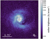 |
Fig. 1 SPHERE H-band Qϕ final image obtained from the DPI data. The red dashed circle represents the radius found from ALMA data. The green crossindicates the position of the point source candidate described in this paper (see Sect. 4.1). The gray hashed circle in the image center marks the size of the coronagraph. No deprojection to the disk plane was applied to this image. |
3.2 SPHERE/VLT total intensity imaging
The second epoch observation of DR Tau with SPHERE was performed on the night of 28 November 2019 in the context of the SHINE (SpHere INfrared survey for Exoplanets; Chauvin et al. 2017; Desidera et al. 2021; Langlois et al. 2021; Vigan et al. 2021) survey. The observation was performed using the IRDIFS_EXT observing mode with the integral field spectrograph (IFS; Claudi et al. 2008) operating in Y, J, and H spectral bands (between 0.95 and 1.65 μm) and with IRDIS using the K band with the K12 filter pair (wavelength K1 = 2.110 μm; wavelength K2 = 2.251 μm; Vigan et al. 2010).
We also obtained frames with satellite spots that are symmetric with respect to the central star before and after the coronagraphic sequences. This enabled us to determine the position of the star behind the coronagraphic focal plane mask and accurately recenter the data (Langlois et al. 2013). Furthermore, to be able to correctly calibrate the flux of companions, we acquired images with the star off-axis. In these cases, an appropriate neutral density filter was used to avoid saturation of the detector.
The data were reduced through the SPHERE data center (Delorme et al. 2017) by applying the appropriate calibrations following the data reduction and handling (DRH; Pavlov et al. 2008) pipeline. In the IRDIS case, the calibrations included thedark and flat-field correction and the definition of the star center. In addition to the dark and flat-field corrections, IFS calibrations included the definition of the position of each spectra on the detector, the wavelength calibration, and the application of the instrumental flat field. We then applied speckle-subtraction algorithms such as TLOCI (Marois et al. 2014) and the principal component analysis (PCA; Soummer et al. 2012), as implemented in the consortium pipeline application SpeCal (Spectral Calibration; Galicher et al. 2018), to the pre-reduced data. For IFS data, we used the angular-spectral differential imaging (ASDI) PCA approach that uses the 4-ddatacube (spatial dimension, time, and wavelength) as described in Zurlo et al. (2014) and in Mesa et al. (2015).
The final signal-to-noise ratio (S/N) maps obtained from this procedure are shown in Fig. 2 both for IFS (left panel) and IRDIS (right panel). As for the polarimetric data case, we overplot a red circle on both images indicating the radius of the inner dust disk as found by ALMA data. In both images, the white dashed circle indicates the extension of the SPHERE coronagraphfor this observation.
3.3 LMIRCam/LBT data
We also observed DR Tau in the L′ band with LBTI/LMIRCam using the instrument’s non-interferometric, individual-aperture, adaptive-optics imaging mode (Ertel et al. 2020). These observations were executed on the night of 3 March 2020 using only the left side of the LBTI and the Annular Groove Phase Mask (AGPM) coronagraph (Defrère et al. 2014). The observations were performed in pupil stabilized mode to allow us to implement the angular differential imaging (ADI; Marois et al. 2006). The observations were designed to last ~5 hours, but high winds complicated the data acquisition and required the termination of the observation after two hours. The quality of the obtained data was affected by wind shaking the secondary mirror, which rendered the adaptive optics loop unstable and prevented the use of the automated coronagraph centering loop (QACITS approach, Huby et al. 2015); therefore, this step was performed manually with reduced effectiveness.
Basic LBTI calibrations include correlated double sampling, bad pixel correction, and sky background subtraction. The frames were aligned with cross-correlation and centered using a rotationally based centering approach (Morzinski et al. 2015) that utilizes the rotational symmetry of the PSF to determine the star’s location behind the coronagraph. Poor-quality frames (those with less than an 80% maximum cross-correlation with the median pupil of the sequence) were then removed, resulting in ~30% frame rejection. The final dataset that was used for analysis includes 4525 frames covering 75.5° of field rotation. At this stage, synthetic planets were injected (when relevant) using the unsaturated and unocculted PSF of the star to assess the final image sensitivity. The spatial background was further mitigated by subtracting the mode of each column and applying a 15 × 15 pixel high-pass filter. The PSF was then modeled and subtracted using the KLIP algorithm (Soummer et al. 2012) with 10 KL modes over annular segments of 60° azimuthal ranges and a radial range of 10–100 pixels from the image center (~0.1′′–1.1′′). Finally, the frames were derotated and combined using a noise-weighting approach (Bottom et al. 2017). The combined image obtained from this procedure is displayed in Fig. 3, in which we also show the location of the dust disk radius observed by ALMA with a red dashed circle, and the position of the compact feature detected using SPHERE and described in Sect. 4.1 with a red cross. The white dashed circle indicate the location of the AGPM coronagraph used for this observation. No source is detected with S/N ≥ 3.
4 Results
4.1 Disk morphology
The DR Tau circumstellar environment shown in Figs. 1 and 2 is quite complex and can be subdivided in three evident substructures: the inner disk, the spiral arms, and a bright compact structure.
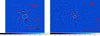 |
Fig. 2 Left: final S/N map obtained from IFS data using the ASDI-PCA and subtracting ten principal components. Right: final S/N map obtained from IRDIS data obtained using the PCA subtracting two principal components. In both images, the red circle represents the disk radius of the inner disk as found with ALMA data, and the red arrow indicates the position of the compact structure described in Sect. 4.1. Moreover, the white dashed circle represents the inner working angle (~0.09′′) of the coronagraph used for these observations. The colour bars below the two images indicates the S/N values obtained from our data reduction procedure. As for the case of Fig. 1, no deprojection to the real orientation of the disk plane was applied to both images. |
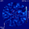 |
Fig. 3 Central part of the signal-to-noise map obtained from the LBTI/LMIRCam data using the KLIP algorithm and subtracting ten modes. The dashed red circle indicates the radius of the dust disk detected with ALMA, while the dashed white circle represents the inner working angle of the AGPM coronagraph (0.09′′). The position of the feature found with the SPHERE data and described in Sect. 4 is marked with a red cross. As forthe case of the SPHERE images, this image has not been deprojected to the disk plane. |
4.1.1 Inner disk
The polarized data (see Fig. 1) show that the inner region just around the star is populated by material (probably both dust grain and gas) at a separation at least larger than the coronagraph inner working angle (i.e., 92.5 mas corresponding to ~18 au at the distance of the system). To the west and to the south of the star, the disk detected in scattered light has a radius comparable to that obtained from submillimeter emission with zero or only faint signal outside this separation.
4.1.2 Spiral arms
We observe a strong emission north- and eastward of the star indicating the presence of a clump of material outside the radius of the disk detected by ALMA. As ALMA is sensitive to millimeter dust grains, this emission could then be dominated by the presence of smaller grains. We note, however, that the ALMA observations presented by Long et al. (2019) are probably not deep enough to reveal extended dust emission at low surface brightness. New deeper ALMA observations will thus be needed for a definitive conclusion on this point.
A spiral pattern starts from the clump described above, and at first look it seems to be composed of a single arm wrapped all around the star (see Fig. 1). However, a more careful analysis reveals that the system is likely composed of at least two different arms. In the left panel of Fig. 4, we display the high-pass-filtered version of Fig. 1 to highlight the presence of these two arms. Their traces are shown by two red dashed lines in the right panel of the same figure for more clarity. The first of these arms starts from north-east of the star at a position angle (PA) of around 20° and moves toward the south, ending south-east of the star at a separation of ~0.8′′ (corresponding to a separation of 154 au at the distance of the system) and a PA of ~ 150°. The second spiral arm departs at a larger separation from the star than the first one (~0.35′′) and it is more wrapped. It starts just south of the star at a PA of ~ 150°, where it is very bright and it wraps around the star toward the west and then to the north fading away while it departs from the star. We are, however, able to trace it up to a separation of 1.14′′ from the star and a position angle of ~ 300°, north-west of the star. This separation is ~220 au at the distance of the system and it is consistent with the size of the gas disk observed by Braun et al. (2021).
Additionally, an arc-like structure is visible north of the star at separations ranging between ~0.63′′ and ~0.73′′ and at PA ranging between around −40° and 33°. Its position is highlighted by a solid red line in the right panel of Fig. 4.
The pitch angle of the two spirals can be determined by transforming the polarized data image in polar coordinates. In this case, the two spiral arms are seen as diagonal lines, and their inclination with respect to the vertical gives their pitch angle. For a nearly face-on disk such as that of DR Tau, this is expected to be rather constant along a spiral arm, except in the close vicinity of an object possibly launching it, though spirals may well be generated by mechanisms other than the presence of a companion. For the north-eastern spiral, we found a moderate pitch angle of ~ 11°, while the southern spiral has a much larger starting pitch angle of ~ 26°, which makes it a very open spiral arm. Additionally, the pitch angle of the second spiral is strongly variable, with values increasing at larger separations and a clear bending toward the north at a separation of ~1.15′′ and at a PA of ~ 260°.
The two spirals are also visible both in IFS and IRDIS total intensity images from the second epoch, even if it is with a very low S/N, as evidenced in Fig. 2. In this case, however, the inner region is completely depleted of any signal. This might indicate that the material in the inner region around the star is strongly polarized.
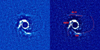 |
Fig. 4 Left: high pass filter of Fig. 1 to highlight the presence of two spirals in the outer part of the disk. Right: same as in the left panel of this figure but with two red dashed lines overplotted to indicate the positions of the two spirals (labeled with NES for the north-eastern spiral and with SS for the southern spiral) and one solid red line to indicate the position of the arc-like structure (labeled with ALS). |
4.1.3 Elongated compact feature
The most striking structure in the total intensity images in Fig. 2 is the elongated compact feature that is clearly visible both in IFS and in IRDIS images north of the star (indicated by a red arrow in both images of Fig. 2). This feature is elongated, especially in the case of the IFS image, so it is difficult to define its position with the usual methods considered for the direct imaging data. However, we applied the negative planet method (Bonnefoy et al. 2011; Zurlo et al. 2014), as implemented in the SpeCal tool, limiting its application to the IRDIS case where the feature is less elongated. We note that the negative planet method assumes that the source is point-like. This is likely not true in this case, but the method can anyhow givea good estimation of the position of the compact structure. From this procedure we obtained a separation of 303 ± 10 mas, corresponding to a projected separation of ~58 au at the distance of the system and a PA of 21.2° ± 3.7°. The unusually high error bars on the SPHERE astrometry reflect the difficulties linked to the elongation of this feature described above.
The compact feature is not visible in Fig. 1 due to the particular contrast settings chosen with the aim of fully displaying the extension of the spiral arms. Figure 5 shows the Qϕ final image adopting different contrast settings. Here, while the spiral arms are barely visible, the feature detected in the total intensity images is obvious, and its position is highlighted by a red arrow. This feature is clearly associated with the region from which the north-eastern spiral is launched, as highlighted by one of the red dashed lines in Fig. 4.
The fact that this feature is quite elongated and is detected both in polarized and non-polarized light indicate that we are probably not directly observing the photosphere of a planet. This is further reinforced by the IFS and IRDIS spectrum extracted using the SpeCal tool and applying the negative planet method. The same limits of this method described above when defining the astrometry of this structure are also valid in this case, but it is useful to give indications about the shape of the spectrum. The results of this procedure are shown in Fig. 6. The S/N of this spectrum is very low, and for a number of wavelengths it was only possible to obtain upper limits. However, the resulting spectrum appears blue, and this is a further indication that we are looking at stellar light reflected by dust.
In principle, with two different epochs separated by nearly one year we could determine the motion of this compact feature. In any case, the astrometric measures are very complicated due to the elongated shape of the structure as explained above. As a consequence, the error bars are very large, so different measures are within error bars each other. Also, the extraction of the astrometric measure from the polarimetric data is further hampered by the noisy environment because of the presence of polarized material around the structure itself. Moreover, we have to consider that the two observations were not done with the same instrumental configuration. In particular, the two IRDIS observations were done at two different spectral bands (H broad-band and K1K2 dual imaging for the polarized and non-polarized observations). The fact that we are observing emission from a dusty environment implies that we are probably observing at a different optical thickness when using different wavelengths. All these considerations make the astrometric comparison of measurements taken at different wavelengths very challenging. We then decided to limit ourselves to the detection of the rotation of this feature comparing the polarimetric data with those from the IFS data, using only the data from the H band part of the spectrum. To this aim, we transformed the two images in polar coordinates, and on these images we performed a cross-correlation to find the relative rotation of one image with respect to the other, masking all but the region around the compact feature. We find a rotation of 1.31° ± 0.08° in the clockwise direction, which is in good agreement with the Keplerian rotation of around 1° expected foran object at the separation of this feature, by adopting the stellar mass from Braun et al. (2021).
To further characterize the environment around DR Tau, we obtained the azimuthal brightness profiles at separations 0.3′′, 0.5′′, 0.7′′, and 0.9′′ from the star with a step of 2° in PA. The results of this procedure are displayed in Fig. 7. The plot obtained at a separation of 0.3′′ is dominated by the peak due to the compact feature described above at a PA of ~ 20° (indicated by a black arrow) while the enhanced flux due to the north-eastern spiral arm is also visible. At larger separations, the azimuthal profiles are dominated by the peaks caused by the southern spiral arm. These peaks of emission are moving west at increasing separation from the star. The feature at a PA of ~ 110°, visible in the plot corresponding to a separation of 0.5′′, might be an extension of the north-eastern spiral arm.
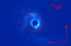 |
Fig. 5 Same Qϕ final image obtained from the DPI data as in Fig. 1 but with different contrast settings and zoomed-in to highlight the presence of the same feature visible in the high-contrast imaging data. The position of the feature is indicated bya red arrow. |
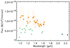 |
Fig. 6 Extracted spectrum of elongated compact structure from IFS and IRDIS data. The orange squares are the IFS data points, and the blue circles are the IRDIS data points. The green upside-down triangles are the upper limits obtained for some wavelengths. |
4.2 Mass limits
We calculated the contrast both for the IRDIS total intensity data and for the LMIRCam data by applying the procedure devised in Mesa et al. (2015). The self-subtraction related to the high-contrast method was estimated injecting simulated planets at different separation in the original dataset and the contrast was then corrected accordingly. Finally, we corrected the results for the small sample statistics following the method described by Mawet et al. (2014). We then transformed these contrast values in mass limits adopting the AMES-DUSTY models (Allard et al. 2001) and an age of 3 Myr. The results are shown in Fig. 8, where we also show the estimated separation from the star of the compact feature with two vertical dashed lines, as described in Sect. 4.1. In both cases, the mass limits are on the order of a few MJup at large separations from the star, while as expected the limits are much lower for the SPHERE data at small separations from the star. We note in any case that the presence of the disk can influence the results, which should be regarded as rough estimates of the limits, especially for the SPHERE case.
5 Discussion
5.1 Origin of the southern spiral arm
A possible explanation for the shape of the spiral arms is that they are due to a companion embedded in the disk. We discuss this possibility for what concerns the north-eastern spiral arm in Sect. 5.2. Concerning the southern spiral arm, we note that the pitch angle of this arm is large (~ 26°) and increases with separation for any possible geometry. A prediction of the models from Bae & Zhu (2018) is that the pitch angle of planet-driven spiral arms decreases with increasing separation from the planet. This would indicate that if the southern spiral arm is generated by a perturbing object, this must be located further than the spiral arm itself. This would imply a separation on the order of more than 200 au for this putative companion. From the mass limit displayed in Fig. 8, we can exclude the presence of objects with masses larger than a few MJup. Companionswith lower masses could, however, be responsible for launching this spiral. In any case, we note that for such low masses the theory of density wave caused by a gravitational perturber in the disk (Rafikov 2002) should be valid, and we should be able to apply the formula defined by Muto et al. (2012) to fit the spiral. However, to be able to fit a spiral with such a high pitch angle, we need to use a very high and unreliable value for the disk aspect ratio. Furthermore, the clear bending toward the north ofthis spiral described in Sect. 4.1.2 makes it very improbable that it could be caused by a single bound object in the disk, but it would require the presence of multiple perturbing objects. These results mean it is unlikely that the southern spiral arm is generated by the perturbation of a planet. The large value of the pitch angle does not agree with predictions for spiral arms caused by shadows either (Montesinos et al. 2016).
As an alternative scenario, spiral arms can be caused by gravitational instability (GI – see e.g., Dong et al. 2015). Through detailed simulations, this study concluded that this mechanism requires the spirals to be relatively compact, on scales of less than 100 au, the disk to be massive and have a mass ratio with the star q larger than 0.1, and the accretion rate to be on the order of 10−6 M⊙ yr−1. These properties do not match the case of the southern arm of DR Tau as it extends out to ~220 au from the star, the stellar mass accretion rate is lower than required (see discussion in Antoniucci et al. 2017), and, moreover, the disk mass is much lower than needed. Ballering & Eisner (2019) estimated a mass of the dust in the disk of log Mdust = −3.53 in solar units. If we adopt the usual dust-to-gas conversion of Mgas∕Mdust = 100, the disk mass is MDisk = 0.03 M⊙, that is q ~ 0.03. The same value is given by Akeson et al. (2019). This is an order of magnitude lower than required for the GI scenario. Furthermore, we could consider the value of the Toomre parameter (Q), which is commonly used to quantify the gravitational disk stability (Toomre 1964). Values of Q above 1.7 are indicative of a stable disk both for linear and second-order perturbations (see e.g., Helled et al. 2014; Sierra et al. 2021). A detailed calculation of this parameter is outside the scope of the present work but we can estimate its value by dividing the disk aspect ratio (H∕R) by the value of q that we define above. A common value of 0.1 for the aspect ratio would imply a value larger than 3 for Q. This put the DR Tau disk into the stability regime. Even if this cannot be considered as a definitive result because of the large uncertainties in this analysis, it is a further indication favoring a stable disk. Finally, simulations show that the number of spiral arms generated in the context of the GI depends on ~ 1∕q (Cossins et al. 2009; Dong et al. 2015; Hall et al. 2019). Considering the value of q ~ 0.03 determined above, we should expect around 30 spiral arms for DR Tau. This is a disk morphology completely different from what our data show. For these reasons, we consider this scenario improbable.
Spirals in a disk may be generated by perturbation by a massive object that had a near encounter (<1000 au) in the recent past (see e.g., Rosotti et al. 2014). An analysis of the Gaia eDR3 proper motion of the other components of the small group in which DR Tau is located allowed us to find the stars that had the nearest approaches in the recent past. We found that there was a passage of DQ Tau at a projected separation of 26 ± 2′′ (corresponding to 5.1 ± 0.3 kau) about 0.231 ± 0.007 Myrs ago. While we can only provide an estimate due to the uncertainties on its proper motion, the close binary V 1001 Tau might have had an even closer encounter with DR Tau, albeit longer ago, passing at a projected separation of only 6′′ (i.e., ~1.1 kau) about 0.850 Myr ago. No other members of the group with entries in Gaia eDR3 passed at shorter distances from DR Tau. In this analysis, we did not consider the component along the line of sight of the velocities as the error bars on the parallax are on the order of 30 μas, which, at the distance of the system, corresponds to ~1.2 pc. This is much larger than the minimum separations we calculated. This makes the use of the velocity along the line of sight unreliable inthis context. While the two passages described above were possibly close enough to trigger a spiral pattern in the DR Tau disk, it is unlikely that this pattern could be visible for such a long time after the passage because of disk viscosity in the inner region, and because the material extracted by the passage would have spread over more than 10 kau after 105 yr (see Rosotti et al. 2014). These results, combined with the lack of any possible close passing object in IRDIS FoV much fainter than detectable by Gaia eDR3 (itself as deep as 20 MJup at separation >3 arcsec), make this explanation for the shape of the spiral pattern unlikely.
A final scenario that we considered requires the presence of infalling material from late encounters of the star with low mass cloudlets as it moves through the molecular cloud in which it formed, as recently proposed by models by, for example, Dullemond et al. (2019) and Kuffmeier et al. (2020). According to what was found by the models cited above, the infalling material might have a very different angular momentum with respect to the star and to the material surrounding it. For this reason, this material would not fall directly onto the star but would orbit around it, leading to the formation of a new disk or to the replenishment of the existing one with a clear misalignment of the new structure with respect to the structures formed during the star formation. The formation of spirals by the infalling material is a natural consequence of this process. The clear changes in surface brightness for the spirals of DR Tau could be due to the fact that the spiral itself is distributed on different planes and with different inclinations with respect to the star. This configuration favors visibility in scattered light and helps explain why the corresponding emission is not detected in the ALMA continuum data (Long et al. 2019), though we notice that material as far from the star as the southern spiral was detected by ALMA in molecular lines (Braun et al. 2021). Moreover, we note that according to the results of the simulations cited previously, not all the material of the cloudlets is captured by the star. This remaining material performs a flyby with curved trajectory around the star that results in an arc-like structure resembling the structure that we actually identified in the polarized data of DR Tau. This is indicated by a solid red line in Fig. 4.
The native environment of DR Tau makes this hypothesis all the more possible. Indeed, the star is located in the close vicinity of Lynds 1558 (Lynds 1962), which is likely the parent cloud of the small association including the star (Lee & Chen 2009). Unfortunately, this region is slightly out of the high-resolution maps obtained with Herschel and described by Roccatagliata et al. (2020). These maps, however show a filamentary structure from north-east to south-west in an adjacent region. At a lower resolution, Fig. 9 shows the environment of DR Tau in the thermal dust emission map from the 2018 version of the Planck Legacy Archive1. From this map, it appears that DR Tau is located at the south-eastern edge of Lynds 1558, in agreement with the idea that the formation of the cloud and of the stars could be triggered by the expansion of the Orion super-bubble (Lee & Chen 2009). Within this environment, late accretion of material onto DR Tau looks highly possible. Even more likely is that this material comes from the north-west, where the densest region of Lynds 1558 is located, but this could only be properly assessed if the relative motions were known.At the moment, this is not possible as the spatial velocities UVW for Lynds 1558 are unknown (e.g., Galli et al. 2019).
All these characteristics of the DR Tau disk tend to favor an interpretation of infalling material responsible for creating at least the southern spiral. The number of spiral disks for which the late infalling of material has been proposed to explain their shape is at the moment small. We can cite AB Aur, HD 100546 (Dullemond et al. 2019), HL Tau (Yen et al. 2019), and SU Aur (Ginski et al. 2021), for example. All these stars have a spiral pattern comparable to that of DR Tau, but, on the other hand, they also have a mass larger than 2 M⊙. According to Dullemond et al. (2019), the presence of such structures around stars with lower masses is less probable. DR Tau should thus be one of the lower mass stars around which these structures are actually present.
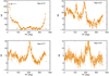 |
Fig. 7 Azimuthal surface brightness profiles obtained around DR Tau using the IRDIS polarized data at separations of 0.3′′ (upper left panel), 0.5′′ (upper right panel), 0.7′′ (bottom left panel), and 0.9′′ (bottom right panel). The black arrow in the top left panel indicates the position of the peak due to the compact feature. The error bars in the 0.3′′ plot are barely visible due to the higher flux scale in that plot with respect to those obtained at larger separations. |
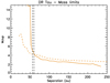 |
Fig. 8 Mass limits around DR Tau as obtained from the LMIRCam L′ data (solid orange line) using the AMES-DUSTY models and assuming a system age of 3 Myr. The dashed orange line represents the limits obtained using the total intensity IRDIS data assuming the same model and the same system age. The two black dashed lines give the estimated separation of the compact feature. |
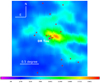 |
Fig. 9 Map of thermal dust emission in direction of DR Tau obtained by Planck including the Lynds 1558 cloud. The color-code represents intensity. Red crosses are positions of stars projected close to DR Tau, which is marked with a red circle; however, only those stars closer to DR Tau are likely members of the small association around DR Tau |
5.2 Nature of the compact feature and the north-eastern spiral arm
As seen above, a compact structure is visible north of the star at both the SPHERE epochs and both in polarized light and in total intensity. This fact makes it very probable that we are looking at a real feature of the disk and not simply at a structure created by the differential imaging data reduction methods. In the polarimetric data, this feature seems connected to the north-eastern spiral arm. While all the results hint toward stellar light reflected by dust, the nature of this bright compact structure is not clear. One intriguing possibility, which is reinforced by the Keplerian motion tentatively detected for this feature by the analysis described in Sect. 4.1, is that it is caused by the presence of a planet in formation and still embedded in its dust envelope.
The characteristics of the feature described in Sect. 4.1 resemble those of one of the two features detected by Boccaletti et al. (2020) in the AB Aur system, whose disk is also characterized by the presence of spiral arms. Indeed, in both cases the feature appears to be elongated, and, due to their detection both in polarized and total intensity light, it is improbable that we are looking at the emission from the photosphere of a planet, at least at the wavelengths imaged by SPHERE. Furthermore, as for the case of AB Aur, this feature is within one of the two spiral arms detected in the disk itself. The most probable explanation for the nature of the feature in AB Aur was that it was caused by a forming planet. However, we note that in that case the authors were able to fit the spiral’s shape with the formula from Muto et al. (2012) while we found that this was not possible for the case of DR Tau. For this reason, the similarity between the two cases should be taken with caution.
In any case, to strengthen the hypothesis of the presence of a companion we can consider the shape of the spiral around the position of the proposed companion. To this aim, we deprojected the image to the plane of the disk using the ALMA values, transformed it into polar coordinates, and for each position angle (with a step of 0.01 radians) we calculated the position of the spiral considering the peak of a Gaussian fit in the radial direction and assuming as error the FWHM of the Gaussian fit. The same procedure was applied both to the IFS Y-H data and to the IRDIS polarized data. In this way it was possible to compare the shape of the spiral in the two epochs after shifting the IFS data by 1.31° to account for the shift between the two epochs measured in Sect. 4.1. Results at different epochs that are displayed in Fig. 10 are very similar to each other, and, more importantly, they both exhibit the S shape that is characteristic of the presence of a companion according to the results of hydrodynamic simulations (see, e.g., Zhu et al. 2015; Bae & Zhu 2018).
If the presence of a companion is the correct explanation for this structure it would be important to estimate its mass. This is, however, a very difficult task given that, as explained before, we are not seeing the planetary photospheredirectly. Since radiation at longer wavelengths is less absorbed or scattered and a small-mass planet is likely very cool, a constraint could be obtained from the mass limit obtained from the observation in the L′ spectral band with LMIRCam described in Sect. 3.3 and shown in Fig. 8 with solid lines. While these results should be taken with some caution due to the poor weather conditions in which the data were taken, they can be useful to give some indication regarding the mass of the putative object. From the plot, it is apparent that the mass of the companion should be less than a few MJup, otherwise it would also be visible in the LMIRCam data.
A further indication that the mass of the companion should be small is that we are not able to detect any gap in the disk in our images of the DR Tau system. The presence of such gap would be requested for a companion with a mass larger than few MJup embedded in the disk according to the formula provided in Kanagawa et al. (2016), for example. However, we note that the ALMA millimeter emission outer radius is inside of the current companion position. In that case, the companion may rather reside on the outside of the dust disk, truncating it. In this case we would not expect to see any gap-like structures. From the ALMA continuum data, it is, however, not clear if the gas disk extends further out than the bulk of the millimeter-sized grains.
We can also use the shape of the north-eastern spiral to confirm this results. Indeed, the radius of the Hill sphere of the proposed companion should be roughly half of the offset in radial position of the leading and trailing part of the spiral arm at its position (Schulik et al. 2020). To take into account the pitch angle, we computed linear fits of the leading and trailing portion of the spiral arm and measured the shift between the two fitting lines at the proposed companion position. We applied this procedure both to IFS H-band data and IRDIS polarized data, as illustrated in Fig. 11, where we represent the spiral points with blue filled circles and the results of the linear fit procedure with red dashed lines. The black arrows represent the measured offset between the inner and the outer part of the spiral. From this procedure, we obtain a value of 22 mas for the Hill radius in the case of the IFS data and of 32 mas in the case of the IRDIS polarized data. We can then assume a value of 27 ± 5 mas for the Hill radius of the proposed companion, which corresponds to a mass of the embedded companion of  MJup if we assume for the stellar mass the value obtained by Braun et al. (2021). In any case, the previous discussion cannot be considered as a precise measure of the Hill radius or, as a consequence, of the mass of the companion. In the case of a small companion not opening a gap, the launching position for a spiral density wave may not be at the separation of the Hill radius but at a separation corresponding to 2/3 of the disk scale height (Fung & Dong 2015), which is larger than the Hill radius of low-mass planets. For this reason, the value obtained using the previous considerations has to be considered as a rough estimation of the mass. In any event, it can give important indications about the order of magnitude of the companion mass, and it is important to confirm that it should be on the order of a few MJup.
Finally, we note that if the embedded companion were more massive than a few Jupiter masses, we should expect to have a symmetric twofold spiral pattern (Bae & Zhu 2018), which in reality we do not see. We conclude that the properties of the compact feature north of the star are compatible with the presence of an embedded planetary mass companion, with a mass of a few Jupiter masses, and that this planet could be responsible for the shape of the north-eastern spiral.
While the evidence presented above seems to point toward a spiral caused by the presence of a planet, we cannot exclude any other possible cause of the formation of the north-eastern spiral. In particular, if, as we discussed in Sect. 5.1, the southern spiral is caused by the late infall of material in the system, we cannot exclude that the north-eastern spiral has also been affected, at least partially, by this process. We could also consider a scenario in which both planetary formation and late infall of material are involved in the definition of the shape of this spiral. In this context, we could explore a scenario that considers the formation and growth of planets in disks with late accretion of material, for example in the context of planetesimals (Pollack et al. 1996), pebbles (see, e.g., Johansen & Lacerda 2010; Bitsch et al. 2019), or hybrid (see, e.g., Alibert et al. 2018) accretion models. While seeds for planet formation are likely needed anyway, they may be much smaller than the final planet and may form closer to the star where timescales for seed core formation are fast enough. During the late infall episodes, the gas and pebble flux may grow considerably, though temporarily, in the outer regions, favoring core growth and thus gas runaway accretion. Of course, these scenarios are complicated by further migration due to interaction between the planet and the disk and by planet-planet scattering; however, in favorable circumstances they might lead to the formation of giant planets at large separations. Due to the large uncertainties, such scenarios can only be supported by a snapshot observation of the process while in progress.
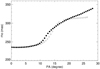 |
Fig. 10 Polar coordinates of eastern spiral arm around the position of the compact feature. The full circles represent the positions obtained with IFS data, while the empty diamonds represent the positions obtained with the IRDIS polarized data. Error bars are too small with respect to the scale of the plot and are not visible. |
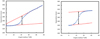 |
Fig. 11 Linear fit (dashed red lines) of the inner and of the outer part of the westward spiral (blue filled circles). The black arrow indicates the offset between the two linear fits. The procedure is illustrated both for the IFS H spectral band data (left panel) and for the IRDIS polarized data (right panel). |
6 Conclusions
We present new observations of the DR Tau system with both SPHERE at VLT and with LBTI/LMIRCam at LBT. The main results obtained from the analysis of these data are summarized here.
The SPHERE polarized data in the H band allowed us to detect a previously undetected system of two spirals around this star, north-east and south of the star,respectively. The same spirals are also visible in the total intensity SPHERE data, albeit with much lower signal-to-noise.
According to our analysis, the most probable origin of the southern spiral is late infalling material from cloudlets present in the formation environment of the star. The presence of a clear arc-like structure just north of the star is a further confirmation of this possibility, as this structure is also foreseen in this scenario. Moreover, we excluded other possible scenarios to explain this spiral arm with a good degree of certainty.
On the other hand, the possibility that the north-eastern spiral is caused by the presence of an embedded companion cannot be excluded. A candidate for this explanation is present just north of the star at separation of ~0.3′′, where a compact bright structure is clearly visible in the SPHERE data both in polarized and non-polarized light. This result and the blue SPHERE spectrum of this feature make it probable that we are not seeing the photosphere of a planet but dust illuminated by the light from the central star.
The nature of this compact structure is unclear, but it strongly resembles a feature identified around AB Aur, which also hosts an extended spiral system. In that case, this structure was interpreted as a planet in formation still embedded in its dust envelope.
The planetary nature of this structure is further supported by the S shape of the north-eastern spiral itself in the region just around its position. This shape is in good agreement with that expected around an embedded companion resultingfrom hydrodynamic simulations.
The possibility that the structure of the north-eastern spiral and the compact feature is influenced by late infall as happens for the southern spiral cannot be excluded. We also considered the possibility both processes are involved in this case.
The mass of this putative companion may be up to the order of a few MJup considering the upper limits provided by the L’ observations with LBTI/LMIRCam, according to which a companion with a larger mass should be detected. This result is strengthened by the absence of a clear gap in the disk, which would be opened by a larger mass companion and by the asymmetry of the spiral pattern that would be symmetric in case of a larger mass companion. Finally, an estimation of the Hill radius based on the offset of the spiral around the companion position confirms that the order of magnitude of the companion mass is in the range of a few MJup or less.
While the high spatial resolution offered by SPHERE is crucial in deriving the geometry of the compact feature, observations at longer wavelengths are needed to disentangle light of a possible companion from the dust in which it is embedded. A first attempt in this direction was done with our observations of DR Tau in the L′ band. Unfortunately, and mainly due to poor weather conditions, these observations were not conclusive, resulting in the non-detection of both companion and disk. Future similar observations both with LMIRCam and similar instruments will be very useful to give a conclusive solution to this problem. Finally, we might expect that if really present, the planet should be accreting and possibly detectable through H emission lines (e.g., Wagner et al. 2018b; Haffert et al. 2019). While they may possibly be strongly absorbed by the circumplanetary material in the visible, they might be detectable in the near IR.
We note that if the results of this work were confirmed, DR Tau would be of paramount importance. This system is much younger than PDS 70, which is currently the benchmark for very young planets caught at very early phases of formation. In the case of PDS 70, the mass of the disk of ~ 0.003 M⊙ (Keppler et al. 2018) is an order of magnitude smaller than the total mass of the two planets (Keppler et al. 2018; Mesa et al. 2019), while in the case of DR Tau the mass of the disk of ~ 0.03 M⊙ (Akeson et al. 2019) is an order of magnitude larger than the mass of the possible planet. DR Tau is thus observed in a much earlier phase, consistent with the age estimates for the stars of 6 Myr for PDS 70 (Müller et al. 2018) and < 3 Myr for DR Tau (see Sect. 2). Furthermore, together with AB Aur (Boccaletti et al. 2020) and perhaps HD 100546 (Quanz et al. 2013; Sissa et al. 2018; Dullemond et al. 2019), DR Tau would be one of the few known objects for which ongoing planetary formation and infall of material on the disk might be present at the same time. This may be relevant to understanding how massive planets can form at very large distances from the star. This is notoriously difficult to explain in scenarios where planets form within a given disk, where the total system mass is constant (see, e.g., the discussion in Nielsen et al. 2019). Given its very young age and distance from its star, which has a mass comparable to that of the Sun, the proposed companion of DR Tau would then be an significant challenge with regard to the current scenarios of planet formation.
Acknowledgements
The authors thank the referee for the constructive comments that helped to improve this work. This work has made use of the SPHERE Data Center, jointly operated by OSUG/IPAG (Grenoble), PYTHEAS/LAM/CeSAM (Marseille), OCA/Lagrange (Nice) and Observatoire de Paris/LESIA (Paris). This work has made use of data from the European Space Agency (ESA) mission Gaia (https://www.cosmos.esa.int/gaia), processed by the Gaia Data Processing and Analysis Consortium (DPAC, https://www.cosmos.esa.int/web/gaia/dpac/consortium). Funding for the DPAC has been provided by national institutions, in particular the institutions participating in the Gaia Multilateral Agreement. This work was supported by the PRIN-INAF2019 Planetary Systems At Early Ages (PLATEA). This research has made use of the SIMBAD database, operated at CDS, Strasbourg, France. D.M., R.G., S.D., A.Z. acknowledge support from the “Progetti Premiali” funding scheme of the Italian Ministry of Education, University, and Research. A.Z. acknowledges support from the CONICYT + PAI/Convocatoria nacional subvención a la instalación en la academia, convocatoria 2017 + Folio PAI77170087. A.M. acknowledges the support of the DFG priority program SPP 1992 “Exploring the Diversity of Extrasolar Planets" (MU 4172/1-1). C.P. acknowledges financial support from Fondecyt (grant 3 190 691) and financial support from the ICM (Iniciativa Científica Milenio) via the Núcleo Milenio de Formación Planetaria grant, from the Universidad de Valparaíso. T.H. acknowledges support from the European Research Council under the Horizon 2020 Framework Program via the ERC Advanced Grant Origins 83 24 28. SPHERE is an instrument designed and built by a consortium consisting of IPAG (Grenoble, France), MPIA (Heidelberg, Germany), LAM (Marseille, France), LESIA (Paris, France), Laboratoire Lagrange (Nice, France), INAF-Osservatorio di Padova (Italy), Observatoire de Genève (Switzerland), ETH Zurich (Switzerland), NOVA (Netherlands), ONERA (France) and ASTRON (Netherlands), in collaboration with ESO. SPHERE was funded by ESO, with additional contributions from CNRS (France), MPIA (Germany), INAF (Italy), FINES (Switzerland) and NOVA (Netherlands). SPHERE also received funding from the European Commission Sixth and Seventh Framework Programmes as part of the Optical Infrared Coordination Network for Astronomy (OPTICON) under grant number RII3-Ct-2004-001566 for FP6 (2004–2008), grant number 226604 for FP7 (2009–2012) and grant number 312430 for FP7 (2013–2016). The LBT is an international collaboration among institutions in the United States, Italy and Germany. LBT Corporation partners are: The University of Arizona on behalf of the Arizona Board of Regents; Istituto Nazionale di Astrofisica, Italy; LBT Beteiligungsgesellschaft, Germany, representing the Max-Planck Society, The Leibniz Institute for Astrophysics Potsdam, and Heidelberg University; The Ohio State University, representing OSU, University of Notre Dame, University of Minnesota and University of Virginia. The results reported herein benefited from collaborations and/or information exchange within NASA’s Nexus for Exoplanet System Science (NExSS) research coordination network sponsored by NASA’s Science Mission Directorate. K.W. acknowledges support from NASA through the NASA Hubble Fellowship grant HST-HF2-51472.001-A awarded by the Space Telescope Science Institute, which is operated by the Association of Universities for Research in Astronomy, Incorporated, under NASA contract NAS5-26 555.
References
- Akeson, R. L., Jensen, E. L. N., Carpenter, J., et al. 2019, ApJ, 872, 158 [Google Scholar]
- Alencar, S. H. P., Johns-Krull, C. M., & Basri, G. 2001, AJ, 122, 3335 [NASA ADS] [CrossRef] [Google Scholar]
- Alibert, Y., Venturini, J., Helled, R., et al. 2018, Nat. Astron., 2, 873 [NASA ADS] [CrossRef] [Google Scholar]
- Allard, F., Hauschildt, P. H., Alexander, D. R., Tamanai, A., & Schweitzer, A. 2001, ApJ, 556, 357 [Google Scholar]
- Andrews, S. M., Rosenfeld, K. A., Kraus, A. L., & Wilner, D. J. 2013, ApJ, 771, 129 [Google Scholar]
- Andrews, S. M., Huang, J., Pérez, L. M., et al. 2018, ApJ, 869, L41 [NASA ADS] [CrossRef] [Google Scholar]
- Antoniucci, S., Nisini, B., Biazzo, K., et al. 2017, A&A, 606, A48 [NASA ADS] [CrossRef] [EDP Sciences] [Google Scholar]
- Avenhaus, H., Quanz, S. P., Schmid, H. M., et al. 2017, AJ, 154, 33 [Google Scholar]
- Bae, J., & Zhu, Z. 2018, ApJ, 859, 119 [Google Scholar]
- Ballering, N. P., & Eisner, J. A. 2019, AJ, 157, 144 [Google Scholar]
- Banzatti, A., Meyer, M. R., Manara, C. F., Pontoppidan, K. M., & Testi, L. 2014, ApJ, 780, 26 [Google Scholar]
- Baraffe, I., Homeier, D., Allard, F., & Chabrier, G. 2015, A&A, 577, A42 [NASA ADS] [CrossRef] [EDP Sciences] [Google Scholar]
- Bast, J. E., Brown, J. M., Herczeg, G. J., van Dishoeck, E. F., & Pontoppidan, K. M. 2011, A&A, 527, A119 [NASA ADS] [CrossRef] [EDP Sciences] [Google Scholar]
- Bertout, C., Basri, G., & Bouvier, J. 1988, ApJ, 330, 350 [Google Scholar]
- Béthune, W., Lesur, G., & Ferreira, J. 2017, A&A, 600, A75 [NASA ADS] [CrossRef] [EDP Sciences] [Google Scholar]
- Beuzit, J. L., Vigan, A., Mouillet, D., et al. 2019, A&A, 631, A155 [NASA ADS] [CrossRef] [EDP Sciences] [Google Scholar]
- Bitsch, B., Izidoro, A., Johansen, A., et al. 2019, A&A, 623, A88 [NASA ADS] [CrossRef] [EDP Sciences] [Google Scholar]
- Boccaletti, A., Di Folco, E., Pantin, E., et al. 2020, A&A, 637, L5 [NASA ADS] [CrossRef] [EDP Sciences] [Google Scholar]
- Bonnefoy, M., Lagrange, A. M., Boccaletti, A., et al. 2011, A&A, 528, L15 [NASA ADS] [CrossRef] [EDP Sciences] [Google Scholar]
- Bottom, M., Ruane, G., & Mawet, D. 2017, Res. Notes Am. Astron. Soc., 1, 30 [Google Scholar]
- Braun, T. A. M., Yen, H.-W., Koch, P. M., et al. 2021, ApJ, 908, 46 [NASA ADS] [CrossRef] [Google Scholar]
- Brown, L. R., Troutman, M. R., & Gibb, E. L. 2013, ApJ, 770, L14 [NASA ADS] [CrossRef] [Google Scholar]
- Brown-Sevilla,S. B., Keppler, M., Barraza-Alfaro, M., et al. 2021, A&A, 654, A35 [NASA ADS] [CrossRef] [EDP Sciences] [Google Scholar]
- Chauvin, G., Desidera, S., Lagrange, A. M., et al. 2017, in SF2A-2017: Proceedings of the Annual meeting of the French Society of Astronomy and Astrophysics, eds. C. Reylé, P. Di Matteo, F. Herpin, E. Lagadec, A. Lançon, Z. Meliani, & F. Royer, Di [Google Scholar]
- Chavarria-K., C. 1979, A&A, 79, L18 [NASA ADS] [Google Scholar]
- Chen, C. H., Pecaut, M., Mamajek, E. E., Su, K. Y. L., & Bitner, M. 2012, ApJ, 756, 133 [NASA ADS] [CrossRef] [Google Scholar]
- Claudi, R. U., Turatto, M., Gratton, R. G., et al. 2008, SPIE Conf. Ser., 7014, 70143E [Google Scholar]
- Cossins, P., Lodato, G., & Clarke, C. J. 2009, MNRAS, 393, 1157 [Google Scholar]
- de Boer, J., Langlois, M., van Holstein, R. G., et al. 2020, A&A, 633, A63 [NASA ADS] [CrossRef] [EDP Sciences] [Google Scholar]
- Defrère, D., Absil, O., Hinz, P., et al. 2014, SPIE Conf. Ser., 9148, 91483X [Google Scholar]
- Delorme, P., Meunier, N., Albert, D., et al. 2017, in SF2A-2017: Proceedings of the Annual meeting of the French Society of Astronomy and Astrophysics, eds. C. Reylé, P. Di Matteo, F. Herpin, E. Lagadec, A. Lançon, Z. Meliani, & F. Royer, Di [Google Scholar]
- Desidera, S., Chauvin, G., Bonavita, M., et al. 2021, A&A, 651, A70 [EDP Sciences] [Google Scholar]
- Dohlen, K., Langlois, M., Saisse, M., et al. 2008, SPIE Conf. Ser., 7014, 70143L [Google Scholar]
- Dong, R., Hall, C., Rice, K., & Chiang, E. 2015, ApJ, 812, L32 [Google Scholar]
- Dong, R., Zhu, Z., Fung, J., et al. 2016, ApJ, 816, L12 [Google Scholar]
- Dullemond, C. P., Küffmeier, M., Goicovic, F., et al. 2019, A&A, 628, A20 [NASA ADS] [CrossRef] [EDP Sciences] [Google Scholar]
- Ertel, S., Hinz, P. M., Stone, J. M., et al. 2020, SPIE Conf. Ser., 11446, 1144607 [Google Scholar]
- Facchini, S., Juhász, A., & Lodato, G. 2018a, MNRAS, 473, 4459 [Google Scholar]
- Facchini, S., Pinilla, P., van Dishoeck, E. F., & de Juan Ovelar, M. 2018b, A&A, 612, A104 [NASA ADS] [CrossRef] [EDP Sciences] [Google Scholar]
- Fedele, D., Tazzari, M., Booth, R., et al. 2018, A&A, 610, A24 [NASA ADS] [CrossRef] [EDP Sciences] [Google Scholar]
- Feiden, G. A. 2016, A&A, 593, A99 [NASA ADS] [CrossRef] [EDP Sciences] [Google Scholar]
- Feldt, M., Olofsson, J., Boccaletti, A., et al. 2017, A&A, 601, A7 [NASA ADS] [CrossRef] [EDP Sciences] [Google Scholar]
- Flock, M., Ruge, J. P., Dzyurkevich, N., et al. 2015, A&A, 574, A68 [NASA ADS] [CrossRef] [EDP Sciences] [Google Scholar]
- Fung, J., & Dong, R. 2015, ApJ, 815, L21 [NASA ADS] [CrossRef] [Google Scholar]
- Gaia Collaboration (Brown, A. G. A., et al.) 2021, A&A, 649, A1 [NASA ADS] [CrossRef] [EDP Sciences] [Google Scholar]
- Galicher, R., Boccaletti, A., Mesa, D., et al. 2018, A&A, 615, A92 [NASA ADS] [CrossRef] [EDP Sciences] [Google Scholar]
- Galli, P. A. B., Loinard, L., Bouy, H., et al. 2019, A&A, 630, A137 [NASA ADS] [CrossRef] [EDP Sciences] [Google Scholar]
- Ginski, C., Facchini, S., Huang, J., et al. 2021, ApJ, 908, L25 [NASA ADS] [CrossRef] [Google Scholar]
- Gotz, W. 1980, Inform. Bull. Variable Stars, 1747, 1 [NASA ADS] [Google Scholar]
- Grankin, K. N., Melnikov, S. Y., Bouvier, J., Herbst, W., & Shevchenko, V. S. 2007, A&A, 461, 183 [NASA ADS] [CrossRef] [EDP Sciences] [Google Scholar]
- Gratton, R., Ligi, R., Sissa, E., et al. 2019, A&A, 623, A140 [NASA ADS] [CrossRef] [EDP Sciences] [Google Scholar]
- Gressel, O., Nelson, R. P., Turner, N. J., & Ziegler, U. 2013, ApJ, 779, 59 [NASA ADS] [CrossRef] [Google Scholar]
- Groff, T. D., Kasdin, N. J., Limbach, M. A., et al. 2015, SPIE Conf. Ser., 9605, 96051C [NASA ADS] [Google Scholar]
- Haffert, S. Y., Bohn, A. J., de Boer, J., et al. 2019, Nat. Astron., 3, 749 [Google Scholar]
- Hall, C., Dong, R., Rice, K., et al. 2019, ApJ, 871, 228 [CrossRef] [Google Scholar]
- Helled, R., Bodenheimer, P., Podolak, M., et al. 2014, Protostars and Planets VI, eds. H. Beuther, R. S. Klessen, C. P. Dullemond, & T. Henning, 643 [Google Scholar]
- Herbig, G. H. 1989, in European Southern Observatory Conference and Workshop Proceedings, 33, 233 [Google Scholar]
- Hinz, P. M., Defrère, D., Skemer, A., et al. 2016, SPIE Conf. Ser., 9907, 990704 [Google Scholar]
- Huby, E., Baudoz, P., Mawet, D., & Absil, O. 2015, A&A, 584, A74 [NASA ADS] [CrossRef] [EDP Sciences] [Google Scholar]
- Isella, A., Huang, J., Andrews, S. M., et al. 2018, ApJ, 869, L49 [NASA ADS] [CrossRef] [Google Scholar]
- Jin, S., Li, S., Isella, A., Li, H., & Ji, J. 2016, ApJ, 818, 76 [CrossRef] [Google Scholar]
- Johansen, A., & Lacerda, P. 2010, MNRAS, 404, 475 [NASA ADS] [Google Scholar]
- Kanagawa, K. D., Muto, T., Tanaka, H., et al. 2016, PASJ, 68, 43 [NASA ADS] [Google Scholar]
- Keppler, M., Benisty, M., Müller, A., et al. 2018, A&A, 617, A44 [NASA ADS] [CrossRef] [EDP Sciences] [Google Scholar]
- Kuffmeier, M., Goicovic, F. G., & Dullemond, C. P. 2020, A&A, 633, A3 [NASA ADS] [CrossRef] [EDP Sciences] [Google Scholar]
- Langlois, M., Vigan, A., Moutou, C., et al. 2013, in Proceedings of the Third AO4ELT Conference, eds. S. Esposito, & L. Fini, 63 [Google Scholar]
- Langlois, M., Gratton, R., Lagrange, A. M., et al. 2021, A&A, 651, A71 [NASA ADS] [CrossRef] [EDP Sciences] [Google Scholar]
- Lee, H.-T., & Chen, W. P. 2009, ApJ, 694, 1423 [NASA ADS] [CrossRef] [Google Scholar]
- Ligi, R., Vigan, A., Gratton, R., et al. 2018, MNRAS, 473, 1774 [Google Scholar]
- Long, F., Herczeg, G. J., Harsono, D., et al. 2019, ApJ, 882, 49 [Google Scholar]
- Lorenzetti, D., Larionov, V. M., Giannini, T., et al. 2009, ApJ, 693, 1056 [NASA ADS] [CrossRef] [Google Scholar]
- Lynds, B. T. 1962, ApJS, 7, 1 [NASA ADS] [CrossRef] [Google Scholar]
- Macintosh, B., Graham, J. R., Ingraham, P., et al. 2014, Proc. Natl. Acad. Sci. U.S.A., 111, 12661 [Google Scholar]
- Maire, A. L., Stolker, T., Messina, S., et al. 2017, A&A, 601, A134 [NASA ADS] [CrossRef] [EDP Sciences] [Google Scholar]
- Marois, C., Lafrenière, D., Doyon, R., Macintosh, B., & Nadeau, D. 2006, ApJ, 641, 556 [Google Scholar]
- Marois, C., Correia, C., Galicher, R., et al. 2014, SPIE Conf. Ser., 9148, 91480U [Google Scholar]
- Marshall, J. P., Moro-Martín, A., Eiroa, C., et al. 2014, A&A, 565, A15 [NASA ADS] [CrossRef] [EDP Sciences] [Google Scholar]
- Mawet, D., Milli, J., Wahhaj, Z., et al. 2014, ApJ, 792, 97 [Google Scholar]
- McClure, M. K. 2019, A&A, 632, A32 [NASA ADS] [CrossRef] [EDP Sciences] [Google Scholar]
- Mesa, D., Gratton, R., Zurlo, A., et al. 2015, A&A, 576, A121 [NASA ADS] [CrossRef] [EDP Sciences] [Google Scholar]
- Mesa, D., Keppler, M., Cantalloube, F., et al. 2019, A&A, 632, A25 [NASA ADS] [CrossRef] [EDP Sciences] [Google Scholar]
- Montesinos, M., Perez, S., Casassus, S., et al. 2016, ApJ, 823, L8 [Google Scholar]
- Morzinski, K. M., Males, J. R., Skemer, A. J., et al. 2015, ApJ, 815, 108 [NASA ADS] [CrossRef] [Google Scholar]
- Müller, A., Keppler, M., Henning, T., et al. 2018, A&A, 617, L2 [Google Scholar]
- Muro-Arena, G. A., Ginski, C., Dominik, C., et al. 2020, A&A, 636, L4 [NASA ADS] [CrossRef] [EDP Sciences] [Google Scholar]
- Muto, T., Grady, C. A., Hashimoto, J., et al. 2012, ApJ, 748, L22 [Google Scholar]
- Nielsen, E. L., De Rosa, R. J., Macintosh, B., et al. 2019, AJ, 158, 13 [Google Scholar]
- Norfolk, B. J., Maddison, S. T., Pinte, C., et al. 2021, MNRAS, 502, 5779 [Google Scholar]
- Pavlov, A., Möller-Nilsson, O., Feldt, M., et al. 2008, in SPIE Conf. Ser., 7019, Advanced Software and Control for Astronomy II, eds. A. Bridger & N. M. Radziwill, 701939 [NASA ADS] [Google Scholar]
- Perrot, C., Boccaletti, A., Pantin, E., et al. 2016, A&A, 590, L7 [NASA ADS] [CrossRef] [EDP Sciences] [Google Scholar]
- Petrov, P. P., Gahm, G. F., Stempels, H. C., Walter, F. M., & Artemenko, S. A. 2011, A&A, 535, A6 [NASA ADS] [CrossRef] [EDP Sciences] [Google Scholar]
- Pohl, A., Pinilla, P., Benisty, M., et al. 2015, MNRAS, 453, 1768 [NASA ADS] [CrossRef] [Google Scholar]
- Pohl, A., Benisty, M., Pinilla, P., et al. 2017, ApJ, 850, 52 [Google Scholar]
- Pollack, J. B., Hubickyj, O., Bodenheimer, P., et al. 1996, Icarus, 124, 62 [NASA ADS] [CrossRef] [Google Scholar]
- Pontoppidan, K. M., Blake, G. A., & Smette, A. 2011, ApJ, 733, 84 [Google Scholar]
- Quanz, S. P., Amara, A., Meyer, M. R., et al. 2013, ApJ, 766, L1 [Google Scholar]
- Rafikov, R. R. 2002, ApJ, 569, 997 [Google Scholar]
- Roccatagliata, V., Franciosini, E., Sacco, G. G., Randich, S., & Sicilia-Aguilar, A. 2020, A&A, 638, A85 [NASA ADS] [CrossRef] [EDP Sciences] [Google Scholar]
- Rosotti, G. P., Dale, J. E., de Juan Ovelar, M., et al. 2014, MNRAS, 441, 2094 [NASA ADS] [CrossRef] [Google Scholar]
- Salyk, C., Lacy, J., Richter, M., et al. 2019, ApJ, 874, 24 [NASA ADS] [CrossRef] [Google Scholar]
- Schulik, M., Johansen, A., Bitsch, B., Lega, E., & Lambrechts, M. 2020, A&A, 642, A187 [NASA ADS] [CrossRef] [EDP Sciences] [Google Scholar]
- Sierra, A., Pérez, L. M., Zhang, K., et al. 2021, ApJS, 257, 14 [NASA ADS] [CrossRef] [Google Scholar]
- Siess, L., Dufour, E., & Forestini, M. 2000, A&A, 358, 593 [Google Scholar]
- Sissa, E., Gratton, R., Garufi, A., et al. 2018, A&A, 619, A160 [NASA ADS] [CrossRef] [EDP Sciences] [Google Scholar]
- Skrutskie, M. F., Jones, T., Hinz, P., et al. 2010, SPIE Conf. Ser., 7735, 77353H [NASA ADS] [Google Scholar]
- Soummer, R., Pueyo, L., & Larkin, J. 2012, ApJ, 755, L28 [Google Scholar]
- Takahashi, S. Z., & Inutsuka, S.-i. 2014, ApJ, 794, 55 [NASA ADS] [CrossRef] [Google Scholar]
- Toomre, A. 1964, ApJ, 139, 1217 [Google Scholar]
- van der Plas, G., Ménard, F., Canovas, H., et al. 2017, A&A, 607, A55 [NASA ADS] [CrossRef] [EDP Sciences] [Google Scholar]
- van Holstein, R. G., Snik, F., Girard, J. H., et al. 2017, in SPIE Conf. Ser., 10400, 1040015 [Google Scholar]
- van Holstein, R. G., Girard, J. H., de Boer, J., et al. 2020, A&A, 633, A64 [NASA ADS] [CrossRef] [EDP Sciences] [Google Scholar]
- Vigan, A., Moutou, C., Langlois, M., et al. 2010, MNRAS, 407, 71 [Google Scholar]
- Vigan, A., Fontanive, C., Meyer, M., et al. 2021, A&A, 651, A72 [EDP Sciences] [Google Scholar]
- Wagner, K., Dong, R., Sheehan, P., et al. 2018a, ApJ, 854, 130 [Google Scholar]
- Wagner, K., Follete, K. B., Close, L. M., et al. 2018b, ApJ, 863, L8 [Google Scholar]
- Yen, H.-W., Gu, P.-G., Hirano, N., et al. 2019, ApJ, 880, 69 [NASA ADS] [CrossRef] [Google Scholar]
- Zhang, K., Blake, G. A., & Bergin, E. A. 2015, ApJ, 806, L7 [Google Scholar]
- Zhu, Z., Dong,R., Stone, J. M., & Rafikov, R. R. 2015, ApJ, 813, 88 [NASA ADS] [CrossRef] [Google Scholar]
- Zurlo, A., Vigan, A., Mesa, D., et al. 2014, A&A, 572, A85 [NASA ADS] [CrossRef] [EDP Sciences] [Google Scholar]
All Tables
All Figures
|
Fig. 1 SPHERE H-band Qϕ final image obtained from the DPI data. The red dashed circle represents the radius found from ALMA data. The green crossindicates the position of the point source candidate described in this paper (see Sect. 4.1). The gray hashed circle in the image center marks the size of the coronagraph. No deprojection to the disk plane was applied to this image. |
| In the text | |
|
Fig. 2 Left: final S/N map obtained from IFS data using the ASDI-PCA and subtracting ten principal components. Right: final S/N map obtained from IRDIS data obtained using the PCA subtracting two principal components. In both images, the red circle represents the disk radius of the inner disk as found with ALMA data, and the red arrow indicates the position of the compact structure described in Sect. 4.1. Moreover, the white dashed circle represents the inner working angle (~0.09′′) of the coronagraph used for these observations. The colour bars below the two images indicates the S/N values obtained from our data reduction procedure. As for the case of Fig. 1, no deprojection to the real orientation of the disk plane was applied to both images. |
| In the text | |
|
Fig. 3 Central part of the signal-to-noise map obtained from the LBTI/LMIRCam data using the KLIP algorithm and subtracting ten modes. The dashed red circle indicates the radius of the dust disk detected with ALMA, while the dashed white circle represents the inner working angle of the AGPM coronagraph (0.09′′). The position of the feature found with the SPHERE data and described in Sect. 4 is marked with a red cross. As forthe case of the SPHERE images, this image has not been deprojected to the disk plane. |
| In the text | |
|
Fig. 4 Left: high pass filter of Fig. 1 to highlight the presence of two spirals in the outer part of the disk. Right: same as in the left panel of this figure but with two red dashed lines overplotted to indicate the positions of the two spirals (labeled with NES for the north-eastern spiral and with SS for the southern spiral) and one solid red line to indicate the position of the arc-like structure (labeled with ALS). |
| In the text | |
|
Fig. 5 Same Qϕ final image obtained from the DPI data as in Fig. 1 but with different contrast settings and zoomed-in to highlight the presence of the same feature visible in the high-contrast imaging data. The position of the feature is indicated bya red arrow. |
| In the text | |
|
Fig. 6 Extracted spectrum of elongated compact structure from IFS and IRDIS data. The orange squares are the IFS data points, and the blue circles are the IRDIS data points. The green upside-down triangles are the upper limits obtained for some wavelengths. |
| In the text | |
|
Fig. 7 Azimuthal surface brightness profiles obtained around DR Tau using the IRDIS polarized data at separations of 0.3′′ (upper left panel), 0.5′′ (upper right panel), 0.7′′ (bottom left panel), and 0.9′′ (bottom right panel). The black arrow in the top left panel indicates the position of the peak due to the compact feature. The error bars in the 0.3′′ plot are barely visible due to the higher flux scale in that plot with respect to those obtained at larger separations. |
| In the text | |
|
Fig. 8 Mass limits around DR Tau as obtained from the LMIRCam L′ data (solid orange line) using the AMES-DUSTY models and assuming a system age of 3 Myr. The dashed orange line represents the limits obtained using the total intensity IRDIS data assuming the same model and the same system age. The two black dashed lines give the estimated separation of the compact feature. |
| In the text | |
|
Fig. 9 Map of thermal dust emission in direction of DR Tau obtained by Planck including the Lynds 1558 cloud. The color-code represents intensity. Red crosses are positions of stars projected close to DR Tau, which is marked with a red circle; however, only those stars closer to DR Tau are likely members of the small association around DR Tau |
| In the text | |
|
Fig. 10 Polar coordinates of eastern spiral arm around the position of the compact feature. The full circles represent the positions obtained with IFS data, while the empty diamonds represent the positions obtained with the IRDIS polarized data. Error bars are too small with respect to the scale of the plot and are not visible. |
| In the text | |
|
Fig. 11 Linear fit (dashed red lines) of the inner and of the outer part of the westward spiral (blue filled circles). The black arrow indicates the offset between the two linear fits. The procedure is illustrated both for the IFS H spectral band data (left panel) and for the IRDIS polarized data (right panel). |
| In the text | |
Current usage metrics show cumulative count of Article Views (full-text article views including HTML views, PDF and ePub downloads, according to the available data) and Abstracts Views on Vision4Press platform.
Data correspond to usage on the plateform after 2015. The current usage metrics is available 48-96 hours after online publication and is updated daily on week days.
Initial download of the metrics may take a while.