| Issue |
A&A
Volume 658, February 2022
|
|
|---|---|---|
| Article Number | A120 | |
| Number of page(s) | 26 | |
| Section | Catalogs and data | |
| DOI | https://doi.org/10.1051/0004-6361/202141819 | |
| Published online | 08 February 2022 | |
Inspection of 19 globular cluster candidates in the Galactic bulge with the VVV survey
1
Departamento de Ciencias Físicas, Facultad de Ciencias Exactas, Universidad Andres Bello, Fernández Concha 700, Las Condes, Santiago, Chile
e-mail: elisaritagarro1@gmail.com
2
Vatican Observatory, Vatican City State 00120, Italy
3
Centro de Astronomía (CITEVA), Universidad de Antofagasta, Av. Angamos 601, Antofagasta, Chile
4
Millennium Institute of Astrophysics, Nuncio Monseñor Sotero Sanz 100, Of. 104, Providencia, Santiago, Chile
5
INAF-Osservatorio Astronomico di Capodimonte, Salita Moiariello 16, 80131 Naples, Italy
6
Instituto de Astronomía, Universidad Católica del Norte, Av. Angamos 0610, Antofagasta, Chile
Received:
17
July
2021
Accepted:
11
November
2021
Context. The census of the globular clusters (GCs) in the Milky Way is still a work in progress. The advent of new deep surveys has made it possible to discover many new star clusters both in the Galactic disk and bulge, but many of these new candidates have not yet been studied in detail, leaving a veil on their true physical nature.
Aims. We explore the nature of 19 new GC candidates in the Galactic bulge by analysing their colour–magnitude diagrams (CMDs) in the near-infrared (NIR) using the VISTA Variables in the Via Láctea Survey (VVV) database. We estimate their main astrophysical parameters: reddening and extinction, distance, total luminosity, mean cluster proper motions (PMs), metallicity, and age.
Methods. We obtain the cluster catalogues including the likely cluster members by applying a decontamination procedure on the observed CMDs based on the vector PM diagrams from VIRAC2. We adopt NIR reddening maps in order to calculate the reddening and extinction for each cluster, and then estimate the distance moduli and heliocentric distances. Metallicities and ages are evaluated by fitting theoretical stellar isochrones. We also calculate their luminosities in comparison with known Galactic GCs.
Results. We estimate a wide reddening range of 0.25 ⩽ E(J − Ks)⩽2.0 mag and extinction 0.11 ⩽ AKs ⩽ 0.86 mag for the sample clusters, as expected in the bulge regions. The range of heliocentric distances is 6.8 ⩽ D ⩽ 11.4 kpc. This allows us to place these clusters between 0.56 and 3.25 kpc from the Galactic centre, assuming R⊙ = 8.2 kpc. Also, their PMs are kinematically similar to the typical motion of the Galactic bulge, apart from VVV-CL160, which shows different PMs. We also derive their metallicities and ages, finding −1.40⩽ [Fe/H] ⩽ 0.0 dex and t ≈ 8 − 13 Gyr respectively. The luminosities are calculated both in Ks- and V-bands, recovering −3.4 ⩽ MV ⩽ −7.5. We also examine the possible RR Lyrae members found in the cluster fields.
Conclusions. Based on their positions, kinematics, metallicities, and ages, and comparing our results with the literature, we conclude that nine candidates are real GCs, seven need more observations to be fully confirmed as GCs, and three candidates are discarded as GCs and appear to be younger open clusters.
Key words: Galaxy: bulge / Galaxy: center / Galaxy: stellar content / globular clusters: general / infrared: stars / surveys
© ESO 2022
1. Introduction
As suggested by the ΛCDM model, globular clusters (GCs) are the first stellar associations formed in the early Universe (Phipps et al. 2019), and therefore their physical properties are strongly linked with those of their host galaxies (Brodie & Strader 2006). These ancient star clusters have survived destruction over long galactic histories to become the fossil relics of the earliest epoch of galaxy formation (Kerber et al. 2019; Ferraro et al. 2021). Consequently, they represent powerful tools with which to investigate the formation and evolution of galaxies. However, the information coming from the analysis of a handful of Milky Way (MW) GCs may still be incomplete, either because some of them are very faint, too small, or widespread, or because they are embedded by dust and thus difficult to find. Indeed, most of the ‘missing’ GCs are likely located in obscured regions close to the Galactic centre or near the Galactic plane on the far side of the Galaxy (Minniti et al. 2017a; Garro et al. 2020, 2021b).
Our main long-term goal is to search for hidden GCs in order to reconstruct the formation history of our Galaxy, focussing on the Galactic bulge. For this purpose, in this paper we deal with the characterisation of 19 GC candidates located towards the MW bulge. This represents a challenge because these regions are affected by differential reddening and high stellar density. The best way to overcome these problems is to use near-infrared (NIR) observations, given that red giant stars have their emission peak in the NIR and the interstellar dust becomes almost transparent at these wavelengths. The identification of new candidates and their subsequent confirmation as real GCs can be facilitated at these spectral regions (for instance UKS 1 and VVV-CL001; Fernández-Trincado et al. 2020 and Fernández-Trincado et al. 2021, just to mention a few). A step forwards has been possible thanks to the VISTA Variables in the Via Láctea (VVV) survey and its eXtension (VVVX). More than 300 candidate star clusters have been discovered in the Galactic bulge and disk but only a fraction of them have been analysed (Froebrich et al. 2007; Borissova et al. 2014; Minniti et al. 2017b, 2021a; Camargo 2018; Palma et al. 2019; Camargo & Minniti 2019; Garro et al. 2020, 2021b; Obasi et al. 2021, just to mention a few).
A variety of techniques have been used in the literature to identify potential star clusters against the background fields and to confirm their true nature. For example, Minniti et al. (2017a) built density maps using only the red giants, and identified the apparent over-densities to mark the location of GC candidates. Identification of the over-densities was done by visual inspection based on the size of each over-density and considering the typical size of known Galactic GCs (∼2 − 5′). Furthermore, these latter authors compared the CMD of potential candidates with those of well-characterised Galactic GCs as well as their respective background fields in order to verify that the cluster red giant branch (RGB) appears tighter than that observed in the background. Another method used to discriminate field stars from cluster candidates is statistical decontamination, as done by Palma et al. (2016), Minniti et al. (2011), and Garro et al. (2021b). In this latter method, the stars of the cluster CMD that fall in the same intervals of colour and magnitude as those of the background CMD are removed.
However, not all over-densities are true clusters; they may simply be groups of stars or statistical fluctuations of the projected stellar density in the plane of the sky (Gran et al. 2019; Palma et al. 2019; Minniti et al. 2021b). Therefore, one of the most reliable methods capable of confirming or discarding the existence of a cluster is the kinematic analysis. Coherent stellar motions ensure the cluster membership, and allow us to separate the stars belonging to an association from those randomly distributed in the field. Several studies (Zoccali et al. 2002; Sariya & Yadav 2015; Baumgardt et al. 2018; Garro et al. 2020, 2021b; Obasi et al. 2021; Minniti et al. 2021a, just to mention a few) have incorporated this technique, especially exploiting the high precision of Gaia proper motions (PMs), confirming, in many cases, the GC nature of some objects. Complementary evidence in support of the cluster identification is the presence of RR Lyrae stars, which are good tracers of old stellar populations (e.g., Minniti et al. 2017b).
In Sect. 2, we briefly describe the datasets used in this work. In Sect. 3, we describe the decontamination procedure, and the two tests performed in order to confirm the existence of the cluster. The methods to estimate the main physical parameters are explained in Sect. 4. In Sect. 5, we present the results of our search for RR Lyrae stars belonging to the clusters in order to confirm the GC nature. A comparison with the literature and final notes are reported in Sect. 6 and a summary and conclusions are presented in Sect. 7.
2. Observational dataset
We use the NIR dataset from the VVV survey (Minniti et al. 2010; Saito et al. 2012), which was acquired with the VISTA InfraRed CAMera (VIRCAM) at the 4.1m wide-field Visible and Infrared Survey Telescope for Astronomy (VISTA; Emerson & Sutherland 2010) at ESO Paranal Observatory. The VVV data were reduced at the Cambridge Astronomical Survey Unit (Irwin et al. 2004) and further processing and archiving was performed with the VISTA Data Flow System (Cross et al. 2012) by the Wide-Field Astronomy Unit and made available at the VISTA Science Archive. We use preliminary data from VIRAC version 2 (VIRAC-2; Smith et al. 2017), which is described in detail in Smith et al. (in prep.). In summary, VIRAC-2 identifies the sources in the VVV images and extracts their photometry through point spread function (PSF)-fitting techniques using DoPhot (Schechter et al. 1993; Alonso-García et al. 2012, 2018). Their astrometry is calibrated to the Gaia DR2 (Gaia Collaboration 2018b) astrometric reference system, and their photometry is calibrated in the VISTA magnitude system (González-Fernández et al. 2018) against the Two Micron All Sky Survey (2MASS; Skrutskie et al. 2006) using a globally optimised model of frame-by-frame zero points plus an illumination correction.
We use also the 2MASS catalogue in order to include brighter stars with Ks < 11 mag, because these stars are saturated in the VVV images. Additionally, we transformed the 2MASS photometry into the VISTA magnitude scale (González-Fernández et al. 2018), because the magnitude scale is different in the two photometric systems.
Moreover, we also explore the optical Gaia Early Data Release 3 (EDR3; Gaia Collaboration 2021) for eight GC candidates: FSR 0009, FSR 1775, VVV-CL131, VVV-CL143, ESO 393-12, ESO 456-09, DB044, and Kronberger 49, for which we obtain suitable CMDs and reliable physical parameters. Nevertheless, we cannot use the Gaia EDR3 data for the other targets because the CMDs are largely affected by the differential reddening, which distorts all optical evolutionary sequences. For this purpose, we use the contaminated VVV-CL150 field as representative, making a comparison between the NIR and optical wavelengths in order to show how the dust is opaque in the optical image and does not allow seeing beyond; also, it distorts the VVV-CL150 CMD, as demonstrated by Fig. 1. For that reason, we cannot use the optical Gaia EDR3 dataset for the other star clusters.
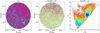 |
Fig. 1. VVV (on the left) and Gaia+VVV (in the middle) density maps for a r = 10′ field centred on VVV-CL150, which is used as a representative cluster. The redder areas are representative of over-densities, while the yellower areas are lower densities. The Gaia EDR3 + VVV CMD (on the right) is displayed for the same field. |
3. Proper motion decontamination procedure
We investigated 19 GC candidates that are located towards the Galactic bulge and are situated within a projected angular distance of 10° from the Galactic centre, as shown in Fig. 2. For the VVV, 2MASS, and Gaia EDR3 data, we performed a decontamination procedure in order to build a clean, decontaminated catalogue of probable cluster members following the same procedure applied by Garro et al. (2020, 2021b).
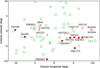 |
Fig. 2. Map depicting Galactic latitude versus longitude for our sample. The confirmed GCs are highlighted as red points, whereas transparent red points are used to point out the unconfirmed GCs. We also mark with open red circles the open clusters excluded from our analysis. We show known GGs from Vasiliev & Baumgardt (2021) with open green squares for comparison. We use shorter cluster identifications only for our convenience. |
Briefly, we underline the main steps taken to obtain the final cluster catalogues. First of all, we include all stars with parallax values smaller than 0.5 mas, discarding all nearby stars. It is very difficult to derive the sizes of the clusters, especially in such crowded regions and for very weak clusters. For that reason, we derive the cluster size using two methods: (i) we inspect the density diagrams as a function of sky position in order to visually identify the cluster dimensions, and (ii) we apply the Gaussian kernel density estimate (KDE; e.g., Rosenblatt 1956; Parzen 1962). In summary, considering the scatter plot on the left-hand side of Fig. 3, overlapping points make the figure hard to read. Even worse, it is impossible to determine how many data points are in each position. In this case, a possible solution is to cut the plotting window into several bins (100–300 bins), and colour code the number of data points in each bin. Following the shape of the bin, this makes a 2D histogram. It is then possible to obtain a smoother result using the Gaussian KDE. Its representation is called a 2D density plot, and we add a contour to denote each density step. We use both density maps and KDE contours to identify the optimal cluster size, selecting the higher density area around the cluster centre. Therefore, we select all stars within the typical GC radius r < 3′ from the cluster centre, although we adopt a smaller radius r < 1.8′ for the cluster VVV-CL153, and a larger radius for the clusters FSR 0009 and VVV-CL154, r < 3.6′ and r < 4.2′, respectively. We then construct and inspect the vector PM diagram (VPM) as a 2D histogram of the relative cluster PMs, as shown in Fig. A.1. Given that our decontamination procedure is based on the PM selection, we also construct histograms of PM in RA (μα*, blue histograms) and in Dec (μδ, red histograms) to clearly recognise the peak (against the noise) of the two distributions. We then visually identify the cluster peak in the VPM diagram, estimating the mean cluster PMs using the σ-clipping technique. All mean cluster PMs are kinematically in agreement with that of the Galactic bulge, except VVV-CL160 which deviates from the typical bulge values (Minniti et al. 2021a). The mean PMs for our GC sample are shown in Fig. 4 (highlighted with red circles), along with the mean PMs of all other known MW bulge GCs measured by Vasiliev & Baumgardt (2021). Indeed, this figure illustrates that the new GCs show kinematics that are akin to the rest of the MW GCs. Finally, we select all stars within 1.0, 1.5, or 2.0 mas yr−1 from the mean cluster PMs. The choices to adopt different radii and PM selections (σPM) for all star clusters are motivated by the intention to only select stars that are likely members of the clusters in order to minimise the likelihood of including outer stars and excluding member stars. A preliminary step, made exclusively for clusters analysed in the optical passband, is to join the Gaia EDR3 and VVV datasets (using a 0.5″ matching radius) before the decontamination procedure mentioned above. The positions, radii, and PM selections are summarised in Table 1 for every candidate.
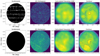 |
Fig. 3. KDE technique applied to select the likely size of a cluster during the decontamination procedure. From left to right: scatterplot, 2D Histogram, Gaussian KDE, and 2D density with contours are shown for FSR 1767 (top panels) and VVV-CL160 (bottom panels) fields, which are used as representative. Green and yellow areas are illustrative of over-densities, while the blue areas show lower densities. |
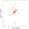 |
Fig. 4. Vector PMs shown to demonstrate that the kinematics of the star clusters analysed here are consistent with those of the known GCs located in the direction of the MW bulge. Our targets are highlighted with red points, whereas the known GCs located in the bulge within −10 < l(deg) < 10 and −10 < b(deg) < 10 are represented by open green squares. |
Position selection cuts for the PM-decontamination procedure, and mean cluster PMs for the GC candidates.
Finally, we perform two tests in order to confirm that our targets are real clusters, even if they have previously been catalogued as such in the literature (see Sect. 6). First, we compare the spatial distribution (Fig. 5) of our clusters (using the decontaminated catalogues) with those of a sample of field stars (cleaned by nearby stars) selected at 5′≲r ≲ 8′ from the relative centre of the cluster. We apply the KDE technique again in order to highlight over-densities. Clearly, the spatial distributions between the clusters and the fields are very different, because a clear central over-density is visible for each cluster, which decreases towards the cluster outskirts; on the other hand, a lumpy and inhomogeneous distribution is seen for the fields, as expected. However, as we can appreciate from Fig. 5, the central over-density is unequivocal for ESO 456-09 (Fig. 5a), VVV-CL160 (Fig. 5c), and VVV-CL150 (Fig. 5d), but is less clear for VVVCL-131 (Fig. 5b). This is related to the fact that some of these clusters have a sparse distribution, as they probably survived dynamical processes, typical of regions of high density such as the Galactic bulge.
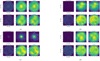 |
Fig. 5. Spatial distribution for four clusters (on the top) and their relative fields (on the bottom) selected at 5′≲r ≲ 8′ from the cluster centre, taken as representative. We use the KDE technique, as in Fig. 3, in order to better distinguish the over-densities (yellow/green colours) from lower-densities (blue colours). (a) ESO 456-09, (b) VVV-CL131, (c) VVV-CL160, (d) VVV-CL150. |
As a second test, we compare our sample with field stars constructing both PM histograms and CMDs (Fig. 6). We expect that field samples include bulge+disk stars, but it is very difficult to split them and to treat them separately, because bulge and disk stars may have similar motions. As done for the clusters, we perform the σ-clipping technique in order to derive the mean field PMs listed in Table 2. We find that the means of the PMs do not differ significantly from those of the clusters, but they show much larger dispersions than the cluster sample, as expected. In this case, the CMDs represent powerful tools to indicate if a star cluster is present or not. Indeed, comparing the clusters and field CMDs, many features, such as red clump (RC), the narrow RGB, and the RGB-bump (RGBB) are clear in many cluster CMDs, while they are not visible in any field CMD. Therefore, all these features strongly support the real cluster nature of our objects.
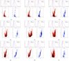 |
Fig. 6. Normalised PM histograms and CMDs for field (in red) and cluster (in blue) stars. We fit the Gaussian distributions (dashed lines) using means and standard deviations listed in Table 2. (a) FSR 0009, (b) FSR 1775, (c) FSR 1767, (d) VVV-CL110, (e) VVV-CL119, (f) VVV-CL128, (g) VVV-CL131, (h) VVV-CL143, (i) VVV-CL150 (j) VVV-CL153, (k) VVV-CL154, (l) VVV-CL160, (m) ESO 393-12, (n) ESO 456-09, (o) DB 044, (p) Kronberger 49. |
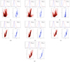 |
Fig. 6. continued. |
PMs comparison between field and cluster stars.
4. Estimation of physical parameters
As shown in Fig. 2, the closest cluster is VVV-CL154 situated within 2.5° of the Galactic centre, while the most distant clusters are FSR 0009, BICA 523, and 524. These regions are strongly affected by stellar crowding and interstellar extinction, which impact the CMDs. Therefore, in order to overcome some of these difficulties, we estimate the reddening and the extinction towards the clusters following Ruiz-Dern et al. (2018). Indeed, we first construct the cluster luminosity functions (Fig. 7) in order to clearly distinguish the RC position, as the peak of the distribution, and then we assign the RC magnitude error as the average of the Ks magnitude errors at the RC level. After that, we use the mean magnitude of RC stars in the NIR from Ruiz-Dern et al. (2018). Their absolute magnitude in the Ks-band is MKs = −1.605 ± 0.009 mag and the intrinsic colour is (J − Ks)0 = 0.66 ± 0.02 mag, whereas for the optical wavebands their intrinsic RC magnitude is MG = 0.459 ± 0.009 mag. Additionally, we adopt the following relations for the extinctions and reddenings: AKs = 0.428 × E(J − Ks) (because our targets are located in the inner Galactic regions, Alonso-García et al. 2017), AKs = 0.11 × AV, AG = 0.86 × AV and AG = 2.0 × E(BP − RP) (Wang & Chen 2019). Also, we derive the colour excess for the optical passband comparing the cluster colours with the absolute colour by Gaia Collaboration (2018a). As expected, the cluster fields exhibit a large range of extinction 0.11 ≤ AKs ≤ 0.86 mag as well as a large range of reddening 0.25 ≤ E(J − Ks)≤2 mag in the NIR, demonstrating again that the reddening is not uniform, which translates into uncertainties in the calculation of the main physical parameters. For example, VVV-CL128, CL150, and CL154 have wide RGBs due to differential reddening and/or residual contamination, as we can see from our CMDs (Fig. A.2). The final reddenings obtained from the CMDs are listed in Table 3. We also compare our reddenings with the high-resolution reddening map by Surot et al. (2020), finding excellent agreement (0.2 ≲ E(J − Ks)≲2.0 mag). Figure 8 shows the de-reddened CMDs for the field stars and FSR 1767, which we take as a representative sample cluster. We selected: (i) field stars in an adjacent area (5′≲r ≲ 8′ from the cluster centre), cleaned by nearby stars; and (ii) PM members of FSR 1767. Comparing these two samples, we do not see a very large spread in colour. However, we can see a well-defined RGB sequence, and also the RC and the RGB-bump are visible in the FSR 1767 CMD, which disappear in the field CMD, a feature that is commonly observed among GCs. Clearly, the position of the RC and RGBB could depend on the bin size in the MKs magnitude; however, in the FSR 1767 CMD (see Fig. A.2), a double over-density is clear at the same magnitudes.
 |
Fig. 7. Luminosity functions in Ks-band for each star cluster. Top: densogram used in order to more easily recognise the RC and avoid the binning dependence. The yellow colour depicts the highest density, with density decreasing towards magenta and then dark blue. We use a bin size of 0.1. |
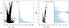 |
Fig. 8. De-reddened CMDs for field stars (on the left) located at 5′≲r ≲ 8′ from the FSR 1767 centre and for the FSR 1767 GC (on the right). We also construct the MKs luminosity function as blue histograms. |
Main physical parameters for each star cluster candidate using the VVV photometry.
Once reddening and extinction are obtained and the RC absolute magnitude by Ruiz-Dern et al. (2018) is taken into account, we are able to derive the distance moduli of the GCs and therefore their heliocentric distances. We find that the distance varies from 6.8 to 11.4 kpc from the Sun. In order to confirm our VVV results, we also report in Table 4 the optical results using the Gaia EDR3 photometry for those clusters for which we obtain suitable Gaia EDR3 data. Furthermore, we use the VVV distances to place our candidates at their respective distances RG from the Galactic centre, assuming that the Sun is located at R⊙ = 8.2 kpc (GRAVITY Collaboration 2019). We find that they are located at Galactocentric distances ranging between 0.56 kpc (for the VVV-CL150) and 3.26 kpc (for the VVV-CL28), as listed in Table 3. Their 3D distribution adopting the Galactocentric coordinates (X, Y, Z) in the Galactic bulge is shown in Fig. 9.
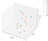 |
Fig. 9. Three-dimensional distribution of the star clusters analysed in this work towards the Galactic bulge using the Galactocentric coordinates (X, Y, Z). The red cross depicts the Galactic centre position at (0, 0, 0). The colour of points indicates the Galactocentric distance (RG in kpc) as specified by the legend. |
Optical parameters derived for those GCs for which it was possible to obtain adequate Gaia EDR3 data, which were used to confirm the VVV results.
Once distances and PMs are known, we can derive their tangential velocities (VT), as shown in Fig. 10. It is clear that their tangential velocities are consistent with those measured by Vasiliev & Baumgardt (2021) for the known GCs located towards the MW bulge. This is further confirmation that they are part of the bulge component.
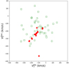 |
Fig. 10. As Fig. 4, we show the star clusters tangential velocities to demonstrate that the kinematics of the star clusters analysed here are consistent with those of the known GCs from Vasiliev & Baumgardt (2021) located in the direction of the MW bulge. |
Using the reddening and distance estimates, we fit the alpha-enriched PARSEC isochrones (Bressan et al. 2012; Marigo et al. 2017) –which reproduce the evolutionary sequences in the observed CMDs slightly better than the solar-scaled model– in order to derive both metallicity and age for our targets. We perform isochrone-fitting, reproducing in particular the position of the RC, blue horizontal branch stars (BHB), and the RGB (Fig. A.2). We compare our evolutionary sequences in the CMDs with the isochrones generated for different ages and metallicities and visually select the best fit. Deriving the metallicity is more straightforward than the age, because metallicity has a particularly significant effect on the evolved sequences (i.e. RC, HB, and RGB). Therefore, first of all we fix the metallicity for each candidate, and then we derive the ages. We find 11 metal-rich GCs with [Fe/H] = 0.0 to −0.6, while 3 are metal-poor GCs with [Fe/H] = −1.2 and −1.4, and 2 show intermediate values of [Fe/H] = −0.7 and −1.1, with a mean error of ±0.2 dex. On the other hand, estimating ages is a challenging task, as one usually needs to reach ∼2 mag below the main sequence turn-off (MSTO) to determine their absolute values. Nevertheless, we are unable to go beyond Ks > 17.5 mag (and G > 17.0 mag), meaning that the MSTO lies below the detection limit. Despite this, we can obtain a robust lower limit for ages, considering three observables from the CMDs. Firstly, we use the vertical method, estimating the difference in magnitude between the HB and the MSTO. In our cases, the ΔKs(HB-MSTO) ≳2 mag, therefore ensuring that our candidates are older than ∼8 Gyr. Secondly, a large extension of the giant branch suggests an intermediate age system, indicating that bright and red stars are present especially along the asymptotic giant branch (Freedman et al. 2020). Also, the presence of RR Lyrae variable stars guarantees that the ages are older than 10 Gyr (Sect. 5).
Most of the analysed clusters show ages that are consistent with the old ages expected for GCs, except for BICA 523 located at RA = 17:14:58.0, Dec = −36:48:28, BICA 524 situated at RA = 17:15:08.0, Dec = −36:47:12, and FSR 0022 placed at RA = 17:56:23.7, Dec = −23:11:35, which are likely open clusters with Age < 6 Gyr (i.e. Salaris et al. 2004). We therefore exclude these latter from further analysis because our main long-term goal is to complete a census of the GCs in the MW.
Furthermore, we derive the global metal content for the sample from the slope of the RGB in order to minimise the effect of age–metallicity degeneracy (e.g., Ferraro et al. 2000; Valenti et al. 2004). We use the [Fe/H]–slope relation by Cohen et al. (2015), finding excellent agreement with our original estimates, within the errors (see Table 3).
After finding the best-fitting age and metallicity simultaneously, we also give an estimation of the age and metallicity errors by varying the parameters until the isochrones are not adequate to reproduce the evolutionary sequences as shown by Fig. A.2. However, it is clear that the correct determination of the age is still one of the most arduous tasks, especially in environments with high stellar density and with differential reddening, and our ages are only rough estimates.
Additionally, we show the Gaia optical CMDs in Fig. 11 and list the physical parameters in Table 4 for the eight GCs for which we also carried out the photometric analysis in the optical passbands. Although it is difficult to simultaneously reproduce all the evolutionary sequences, we notice that both optical and NIR analyses are in good agreement within the errors, confirming the VVV results.
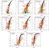 |
Fig. 11. Gaia CMDs for the eight clusters for which we obtain reliable results in the optical passband. The black dotted line depicts the isochrone with the same age and metallicity as the VVV photometry and listed in Table 3. |
Finally, the total luminosities in the Ks-band (MKs) for all the GCs in our sample were derived by first measuring the flux for each star and then the total flux for the cluster. We then converted the latter into the MKs, listed in Table 3. As mentioned above, faint stars below the MSTO are missing in our catalogues, and so the integrated luminosities of our clusters should be considered as lower limits. For this purpose, we compared our GC MKs with other known and well-characterised Galactic GCs listed in Table 5, where we recovered their reddening and distance modulus. We follow the same approach as Garro et al. (2021a). The main goal is to quantify the fraction of luminosity that comes from the faintest stars in order to better estimate the total luminosity of each cluster. We obtain an empirical correction to our cluster’s luminosities under the assumption of similarity among Galactic GCs. We find that most of them are low-luminosity GCs, with MV fainter than the MW globular cluster luminosity function (GCLF) peak (MV = −7.4 ± 0.2 mag; Harris 1991; Ashman & Zepf 1998). On the other hand, there are two GCs with total luminosities comparable with the MW GCLF peak: VVV-CL119 (MV = −7.5) and VVV-CL154 (MV = −7.2).
Known and well-characterised GCs used to derive the total luminosity for each GC.
All their main physical parameters are listed in Table 3, where we summarise the cluster identification (ID), the RC position, the reddening and extinction, the distance, the luminosity, the mean cluster PMs, the metallicity, the age, and the classification type for each candidate.
5. Searching for RR Lyrae stars
We also searched for RR Lyrae stars within a radius of 12′ centred on the clusters (Table B.1), as these variables are good tracers of old populations and are also excellent distance indicators. Our selection includes samples from the Optical Gravitational Lensing Experiment (OGLE; Soszyński et al. 2014), and the VVV (Majaess et al. 2018) and Gaia (Clementini et al. 2019) catalogues. We detect RR Lyrae stars in the fields of FSR 1775 ( ), FSR 1767 (
 ), Kronberger 49 (
 ), ESO 393-12 (
 ), ESO 456-09 (
 ), DB044 (
 ), VVV-CL131 (
 ), VVV-CL143 (
 ), and VVV-CL154 (
 ). The number density of field bulge RRab stars has been estimated by Navarro et al. (2021).
In order to identify RR Lyrae stars belonging to the GCs we mainly rely on two parameters: heliocentric distances and PMs. We use the period–luminosity–metallicity (PLZ) relation in the NIR following Muraveva et al. (2015) (with RRc stars ‘fundamentalized’ by adding 0.127 to the logarithm of the period) to derive their heliocentric distances (DRRLS). After that, we measure their projected distances from the GC centres (Dc), and we construct a DRRLS − Dc diagram as shown in Fig. 12. We then compare the RR Lyrae PMs with the cluster PMs as displayed in Fig. A.2 (left panels), keeping only those stars that have PMs matching the mean cluster PMs within the errors. According to PMs and heliocentric distances, we strictly identify NRRLS(FSR1775) = 2, NRRLS(FSR1767) = 2, NRRLS(Kron49) = 3, NRRLS(ESO393-12) = 3, NRRLS(ESO456-09) = 6, NRRLS(DB044) = 6, NRRLS(VVV-CL131) = 2, NRRLS(VVV-CL143) = 4, and NRRLS(VVV-CL154) = 15, as GC members. We verified our distances using the PL relations from Navarrete et al. (2017) and Gaia Collaboration (2017), yielding slightly larger distance values, and Alonso-García et al. (2021), yielding slightly shorter distance values in the mean. For the latter, we transformed the metallicities listed in Table 3 into log Z using the relation shown in Navarrete et al. (2017), assuming f = 10[α/FeH] = 3 and Z⊙ = 0.017. However, we find that Alonso-García et al. (2021) follows the DB044 and ESO 456-09 RR Lyrae trends better than Muraveva et al. (2015), and so we use the Alonso-García et al. (2021) relation for these clusters. Nevertheless, both relations are still within the mean errors of ∼0.5 kpc obtained by the comparison between these four PLZ relations.
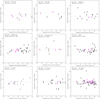 |
Fig. 12. Spatial distribution of RR Lyrae variable stars detected within 12′ from GC centres. The magenta points represent the RR Lyrae that are considered cluster members. The distance error bars are of 0.5 kpc for each point. The dotted line depicts the heliocentric distance derived from the VVV photometry. |
Although these variables are usually found in metal-poor populations, such as Terzan 10 ([Fe/H] = −1.59) and NGC 6656 ([Fe/H] = −1.70), there is evidence (e.g., Alonso-García et al. 2021) of RR Lyrae stars located in metal-rich GCs, such as NGC 6441 ([Fe/H] = −0.46) and Patchick 99 ([Fe/H] = −0.20 – Garro et al. 2021b), as well as in intermediate-metallicity GCs, like 2MASS-GC 02 ([Fe/H] = −1.08) and NGC 6569 ([Fe/H] = −0.76). In our case, we note that the GCs containing RR Lyrae show a metallicity range between −0.6 and −1.2. However, Kronberger 49 with [Fe/H] = −0.2 and DB044 with [Fe/H] = −0.1 could include three and six RR Lyrae members, respectively. Nonetheless, we are careful to state that the three RR Lyrae definitely belong to Kronberger 49 because we have noticed that no PM RR Lyrae matches with cluster PMs within σ < 1 mas yr−1. Also, another caveat is that some variables are situated beyond 5′ from the centre. This means that their position could be beyond the cluster core or tidal radius, suggesting that their membership is less likely. This is the case for VVV-CL143 for example, as the RR Lyrae that could be considered as members are located so far away from the cluster centre that their cluster membership is really unlikely. Regardless, it is very unlikely that clusters with high metallicity host RR Lyrae stars. Hence, we need spectroscopic observations in order to confirm their nature.
Finally, we use these variables to determine the cluster distance independently. We find good agreement between the distances found by the VVV photometry (see Table 3) and the RR Lyrae estimates derived from Muraveva et al. (2015) and Alonso-García et al. (2021) relations: DRRLS(VVV-CL154) = 8.1 kpc, DRRLS(VVV-CL131) = 9.2 kpc, DRRLS(VVV-CL143) = 8.8 kpc, DRRLS(FSR1775) = 9.4 kpc, DRRLS(FSR1767) = 9.4 kpc, DRRLS(ESO393-12) = 7.9 kpc and DRRLS(ESO456-09) = 7.5 kpc. In any case, if we include the Kronberger 49 variables, we find DRRLS(Kron49) = 8.3 kpc, and if we include DB044 RR Lyrae on top of that then we obtain DRRLS(DB044) = 8.0 kpc, both in agreement with the VVV distances.
The magenta squares and points in the CMDs, VPM diagrams, and distance diagrams (Figs. A.2 and 12) depict the RR Lyrae members of each GC.
6. Notes on individual clusters
Below we report on the individual clusters. We display the estimated parameters for each cluster, and we compare our results with those already present in the literature, if any. This helped us to classify our targets as GCs, if possible.
6.1. FSR catalogue
FSR 0009, also referred to as Milky Way Star Cluster (MWSC) 2921, was identified as a Galactic open cluster in the list of Buckner & Froebrich (2013). These authors placed it at equatorial coordinates (J2000) RA = 18:28:32.9, Dec = −31:54:18 and Galactic coordinates l = 1.86, b = −9.52, ∼30″ away from our centre. They concluded that it is a poorly populated cluster with 73 members, its PMs are μα* = 1.25 mas yr−1 and μδ = −6.83 mas yr−1, and its distance is about 3.4 kpc. These results differ from ours, because we find a GC with about 150 stars, with different PMs (see Table 1).
The nature of FSR 1767 has been debated in the past. Froebrich et al. (2007) concluded that it was not a star cluster. Whereas, with 2MASS photometry and PMs, Bonatto et al. (2009) proved that FSR 1767 was a GC located at equatorial coordinates (J2000) RA = 17:35:44.8, Dec = −36:21:42, and Galactic coordinates l = 352.60, b = −02.17, ∼26″ away from our centre. These latter authors suggested that it appears to be a detached post-collapse core, similar to those of other nearby low-luminosity GCs projected towards the bulge. On the other hand, Buckner & Froebrich (2013) classified FSR 1767 as an open cluster with μα* = 0.97 mas yr−1 and μδ = −3.57 mas yr−1, at a distance about 3.6 kpc. They counted 121 members. Our results agree with those of Bonatto et al. (2009) because we classify FSR 1767 as a GC containing about 530 stars, and place it at a distance of ∼10.6 ± 0.2 kpc.
FSR 1775, also named MWSC 2750, was catalogued by Buckner & Froebrich (2013) as a possible open cluster that is poorly populated (52 members) and at equatorial coordinates (J2000) RA = 17:56:07.9, Dec = −36:33:54 and Galactic coordinates l = 354.55, b = −5.79, ∼30″ away from our position space. These latter authors derived PMs of μα* = −9.53 mas yr−1 and μδ = −1.00 mas yr−1 and a distance of 4.6 kpc. Again we obtained different PMs and distances based on about 260 members (see Table 1). In addition, we exclude the open cluster nature because both FSR 1767 and 1775 contain RR Lyrae stars, suggesting relatively old ages.
6.2. VVV catalogue
All clusters named VVV-CL in this work were discovered in the VVV survey by Borissova et al. (2014). We report below our comments on these individual candidates.
VVV-CL110, CL128, CL131, and CL153 are located in VVV tiles b342, b317, b302, and b336, respectively. Borissova et al. (2014) suggest that VVV-CL110, CL128, and CL131 could be GCs or old OCs. We confirm their nature as real GCs. These latter authors suggested that VVV-CL153 could be a prominent bright cluster. Selecting a region of r ≤ 1.8′ from the GC centre and including all stars within 1.5 mas yr−1 from the cluster PMs, we find a relatively dim cluster (MV ≈ −6.8 mag) as indicated by Borissova et al. (2014).
VVV-CL119. Borissova et al. (2014) found this object in VVV tile b344 and classified it as a possible old open cluster. Constructing the CMDs, they located the RC and the TO point at Ks = 13.8 ± 0.2 mag and Ks = 17.3 ± 0.3 mag, respectively. Their main physical parameters are: a mean reddening of E(J − Ks) = 2.03 ± 0.4, a distance modulus of (M − m)0 = 14.17 ± 0.3 (6.8 kpc), an age of 5 ± 1.2 Gyr, and a mean metallicity, calculated from five spectroscopically observed stars of [Fe/H] = −0.3 ± 0.18. The main differences that we notice between our findings and those of this latter work are related to the position of the RC and TO. We identify the RC to be ∼0.7 mag fainter than theirs and we do not reach the MSTO. Although the reddenings are in agreement, we place VVV-CL119 at 11.3 kpc from the Sun, thus ∼4.5 kpc further out than their distance. Finally, the metallicities obtained are in agreement within the errors.
VVV-CL143. This star cluster lies in VVV tile b302. Borissova et al. (2014) identified a defined RGB, several RC stars at Ks = 13.3 ± 0.2 mag, and the TO point at Ks = 16.62 ± 0.3 mag. These authors estimated a reddening of E(J − Ks) = 0.58 ± 0.2, a distance modulus of (M − m)0 = 14.45 ± 0.6 (7.8 kpc), an age of 4 ± 0.7 Gyr, and a mean metallicity of [Fe/H] = −0.62 ± 0.52, which was spectroscopically evaluated from 10 to 12 observed stars. Nevertheless, they were unable to identify the true nature of VVV-CL143, because it could be either a populated old open cluster or a young GC, especially when its relatively low metallicity and CMD morphology are taken into account. We confirm their results because this is a well-populated GC, including 470 stars, with a metallicity of [Fe/H] = −0.6 ± 0.2 at D = 8.9 ± 0.5 kpc and an age of ∼10 Gyr.
VVV-CL150. Borissova et al. (2014) recognised this cluster as a possible new bulge GC, lying in VVV tile b350. Their CMD is well populated and they place the RC at Ks = 13.10 ± 0.2, and the TO at Ks = 17.2 ± 0.4 mag. They calculated reddening of E(J − Ks) = 1.2 ± 0.1, distance modulus of (M − m)0 = 14.22 ± 0.7 (6.98 kpc), age of 10 ± 0.8 Gyr, and metallicity of [Fe/H] = −0.75 ± 0.11. We also obtain similar results in this case. We count 383 stars belonging to VVV-CL150. We do not identify the RC, not even from inspection of the cluster LF, concluding that it is a metal-poor GC with [Fe/H] = −1.30. Also, we find a similar age (12 Gyr) within the errors.
VVV-CL154. Located in VVV tile b321, this object was classified as an old open cluster in close proximity to the Sun, because Borissova et al. (2014) derived a reddening of E(J − Ks) = 1.2 ± 0.1, a distance modulus of (M − m)0 = 10.1 ± 0.3 (1.05 kpc), an age of 8 ± 0.2 Gyr, and a metallicity of [Fe/H]= − 0.69 ± 0.4 from analysis of its CMD. Aside from the metallicity, our estimates are different for this cluster. Our findings indicate an old and distant (∼8.9 kpc) GC located near the Galactic centre (RG = 0.78 kpc).
VVV-CL160. This cluster lies in VVV tile b340. The RGB and MS are well defined in the Borissova CMD, where the RC and TO are identified at Ks = 13.1 ± 0.3 mag and Ks = 14.8 ± 0.4 mag, respectively. Their calculated physical parameters are: reddening E(J − Ks) = 1.72 ± 0.1, distance modulus (M − m)0 = 13.60 ± 0.3 (5.25 kpc), age 1.6 ± 0.5 Gyr, and metallicity [Fe/H]= − 0.72 ± 0.21. Borissova et al. (2014) concluded that VVV-CL160 may be an old metal-poor open cluster. Recently, Minniti et al. (2021a) found a reddening of E(J − Ks) = 1.95 mag, a distance modulus of (m − M)0 = 13.01 mag (4.0 kpc), a metallicity of [Fe/H] = −1.40, an age of 12 Gyr, and a luminosity of MV = −5.1. Interestingly, Minniti et al. (2021a) concluded that VVV-CL160 may belong to a disrupted dwarf galaxy, because the kinematics are similar to those of the known GC NGC 6544 and the Hrid halo stream. Our parameters are in reasonable agreement with both works, as we find a reddening value similar to that of Borissova et al. (2014), while we agree with Minniti et al. (2021a) on the metallicity, luminosity, and age, confirming the GC nature. However, we place this cluster farther than in previous works, at 6.8 kpc from the Sun. Finally, VVV-CL119, CL143, and CL150 were also catalogued as star cluster candidates in the list of Minniti et al. (2017a).
6.3. ESO star cluster candidates
Listed in the Kharchenko et al. (2013) catalogue, ESO 393-12 and ESO 456-9 were recognised as possible globular clusters, located at RA = 17:38:40, Dec = −35:39.0:00 and RA = 17:53:56.4, Dec = −32:27:54, ∼27.40″ and 26.90″ from our positions, respectively. In this work, the PM values are μα* = 4.16 mas yr−1 and μδ = −4.85 mas yr−1 for ESO 393-12, and μα* = 3.83 mas yr−1 and μδ = −10.60 mas yr−1 for ESO 456-09. On the other hand, Dias et al. (2014) catalogued them as open galactic clusters. Our results are inline with those of Kharchenko et al. (2013), as we find two GCs, including RR Lyrae variable stars, which suggests an old age (t > 10 Gyr) for these clusters.
6.4. DB044
DB044 was discovered by Dutra & Bica (2000), who classified this as a possible star cluster. It was further studied by Kharchenko et al. (2013), as a possible open cluster, with PMs of μα* = −6.38 mas yr−1 and μδ = −11.70 mas yr−1. We obtain very different cluster PMs, and we exclude the open cluster nature for two reasons: firstly, because it may include six RR Lyrae stars in its field, and secondly because we derive an age of ∼11 Gyr. Admittedly, this is not a clear case.
6.5. Kronberger 49
Kronberger 49, designed as DSH J1810.3-2320, was discovered by Kronberger et al. (2006). Inspections of DSS/XDSS and 2MASS images revealed a compact object, suggesting that it could be a GC core. Further, Ortolani et al. (2006) observed Kronberger 49 at the Telescopio Nazionale Galileo (TNG) using V, I, and Gunn z photometry, combining them with additional photometry from 2MASS, DENIS, WISE, and VVV surveys. These latter authors analysed the optical decontaminated CMD, where prominent features are a well-defined TO and an RGB with a turnover, suggesting high metallicity. Indeed, the main parameters are a distance modulus of (m − M)V = 18.8, (mM)I = 16.9, and a reddening of E(V − I) = 1.8 (equivalent to E(B − V) = 1.35), and thus a heliocentric distance of d = 8 ± 1 kpc. The absolute magnitude was estimated following two methods based on 2MASS photometry, and Ortolani et al. (2006) calculated MV = −5.4 ± 0.5 and −4.8 ± 0.5. Moreover, they placed Kronberger 49 at 1.2 kpc from the Galactic centre (assuming R⊙ = 8.28 kpc), indicating that it would be an inner bulge cluster. In conclusion, constructing a radial density profile Ortolani et al. (2006) proposed that this cluster might be a core collapse GC, similar to many others in the central part of the MW. They concluded that this is a metal-rich object with [Fe/H] ≈ − 0.1, with an age t ≳ 10 Gyr. We find similarities between the present work and this latter: we place Kronberger 49 at RG = 1.14 from the Galactic centre and at D = 8.3 kpc from the Sun, in agreement with Ortolani et al. (2006). Also, we confirm the metal-rich content and the old age, but we derive a slightly brighter luminosity.
7. Summary and conclusions
In recent decades, many star clusters have been discovered towards the Galactic bulge. However, most of them have not yet been well studied. In this work we study 19 star clusters, recovering their main physical parameters. Reddenings and extinctions along each cluster field are calculated adopting reddening maps in the NIR and measuring the RC position. We also measure their distances using the VVV photometry, including also the Gaia photometry in some cases. Furthermore, we first search for RR Lyrae stars in each cluster field, and we then use the variable star members to estimate the cluster distance as an independent method. Using the isochrone-fitting method with the PARSEC isochrone models we derive their metallicities and ages. We find 11 metal-rich and 3 metal-poor GCs, whereas 2 GCs show intermediate metallicity. We find that the majority of our targets are low-luminosity GCs with MV fainter than the MW GCLF peak.
Dedicated photometric studies spread across the bulge concluded that its mean age is of ∼10 Gyr, and in particular setting a lower limit on ages of 5 Gyr (Clarkson et al. 2011). In this context, we confirm that the clusters studied in this work are members of the Galactic bulge according to their kinematics, positions, ages (t > 8 Gyr), and metallicity range (0.0> [Fe/H] > − 1.40). We also identify three open clusters: FSR 0022, BICA 523, and BICA 524.
In conclusion, we confirm the nature of nine candidates as bona fide GCs: VVV-CL131, VVV-CL143, VVV-CL160, FSR 0009, FSR 1767, FSR 1775, ESO 393-12, ESO 456-09, and Kronberger 49. On the other hand, confirmation of the true nature of the remaining seven candidates requires further investigation, because the effect of the dust strongly reddens their CMDs. This is especially clear in the CMDs of VVV-CL110, CL119, CL128, CL150, and CL153, which show a wider RGB –something that is not typical for bulge GCs– and a poorly defined RC. Therefore, follow-up observations are needed, including spectroscopy in order to measure their kinematics, dynamics, and chemical composition, and deeper imaging to derive their absolute age using the MSTO and calculate their structural parameters.
Acknowledgments
We gratefully acknowledge the use of data from the ESO Public Survey program IDs 179.B-2002 and 198.B-2004 taken with the VISTA telescope and data products from the Cambridge Astronomical Survey Unit. E.R.G. acknowledges support from an UNAB PhD scholarship and ANID PhD scholarship No. 21210330. D. M. acknowledges support by the BASAL Center for Astrophysics and Associated Technologies (CATA) through grant FB 210003. J. A.-G. acknowledges support from Fondecyt Regular 1201490 and from ANID - Millennium Science Initiative Program – ICN12_009 awarded to the Millennium Institute of Astrophysics MAS.
References
- Alonso-García, J., Mateo, M., Sen, B., et al. 2012, AJ, 143, 70 [Google Scholar]
- Alonso-García, J., Minniti, D., Catelan, M., et al. 2017, AJ, 849, L13 [CrossRef] [Google Scholar]
- Alonso-García, J., Saito, R. K., Hempel, M., et al. 2018, A&A, 619, A4 [Google Scholar]
- Alonso-García, J., Smith, L. C., Catelan, M., et al. 2021, A&A, 651, A47 [NASA ADS] [CrossRef] [EDP Sciences] [Google Scholar]
- Ashman, K. M., & Zepf, S. E. 1998, Cambridge Astrophysics Series (Cambridge: Cambridge Univ. Press), 30 [Google Scholar]
- Barbuy, B., Bica, E., Ortolani, S., & Bonatto, C. 2006, A&A, 449, 1019 [NASA ADS] [CrossRef] [EDP Sciences] [Google Scholar]
- Barbuy, B., Muniz, L., Ortolani, S., et al. 2018, A&A, 619, A178 [NASA ADS] [CrossRef] [EDP Sciences] [Google Scholar]
- Baumgardt, H., Hilker, M., Sollima, A., & Bellini, A. 2018, MNRAS, 482, 5138 [Google Scholar]
- Bonatto, C., Bica, E., Ortolani, S., & Barbuy, B. 2009, MNRAS, 397, 1032 [NASA ADS] [CrossRef] [Google Scholar]
- Borissova, J., Chené, A. N., Ramírez Alegría, S., et al. 2014, A&A, 569, A24 [NASA ADS] [CrossRef] [EDP Sciences] [Google Scholar]
- Bressan, A., Marigo, P., Girardi, L., et al. 2012, MNRAS, 427, 127 [NASA ADS] [CrossRef] [Google Scholar]
- Brodie, J. P., & Strader, J. 2006, ARA&A, 44, 193 [Google Scholar]
- Buckner, A. S. M., & Froebrich, D. 2013, MNRAS, 436, 1465 [NASA ADS] [CrossRef] [Google Scholar]
- Camargo, D. 2018, ApJ, 860, L27 [Google Scholar]
- Camargo, D., & Minniti, D. 2019, MNRAS, 484, L90 [Google Scholar]
- Christian, C. A., & Friel, E. D. 1992, AJ, 103, 142 [NASA ADS] [CrossRef] [Google Scholar]
- Clarkson, W. I., Sahu, K. C., Anderson, J., et al. 2011, ApJ, 735, 37 [NASA ADS] [CrossRef] [Google Scholar]
- Clementini, G., Ripepi, V., Molinaro, R., et al. 2019, A&A, 622, A60 [NASA ADS] [CrossRef] [EDP Sciences] [Google Scholar]
- Cohen, R. E., Hempel, M., Mauro, F., et al. 2015, AJ, 150, 176 [NASA ADS] [CrossRef] [Google Scholar]
- Cross, N. J. G., Collins, R. S., Mann, R. G., et al. 2012, A&A, 548, A119 [NASA ADS] [CrossRef] [EDP Sciences] [Google Scholar]
- Dias, W. S., Monteiro, H., Caetano, T. C., et al. 2014, A&A, 564, A79 [NASA ADS] [CrossRef] [EDP Sciences] [Google Scholar]
- Dutra, C. M., & Bica, E. 2000, A&A, 359, L9 [Google Scholar]
- Emerson, J., & Sutherland, W. 2010, Messenger, 139, 2 [Google Scholar]
- Fernández-Trincado, J. G., Minniti, D., Beers, T. C., et al. 2020, A&A, 643, A145 [Google Scholar]
- Fernández-Trincado, J. G., Minniti, D., Souza, S. O., et al. 2021, AJ, 908, L42 [CrossRef] [Google Scholar]
- Ferraro, F. R., Montegriffo, P., Origlia, L., & Fusi Pecci, F. 2000, AJ, 119, 1282 [NASA ADS] [CrossRef] [Google Scholar]
- Ferraro, F. R., Pallanca, C., Lanzoni, B., et al. 2021, Nat. Astron., 5, 311 [Google Scholar]
- Freedman, W. L., Madore, B. F., Hoyt, T., et al. 2020, ApJ, 891, 57 [Google Scholar]
- Froebrich, D., Scholz, A., & Raftery, C. L. 2007, MNRAS, 374, 399 [Google Scholar]
- Gaia Collaboration (Clementini, G., et al.) 2017, A&A, 605, A79 [NASA ADS] [CrossRef] [EDP Sciences] [Google Scholar]
- Gaia Collaboration (Brown, A. G. A., et al.) 2018a, A&A, 616, A1 [NASA ADS] [CrossRef] [EDP Sciences] [Google Scholar]
- Gaia Collaboration (Babusiaux, C., et al.) 2018b, A&A, 616, A10 [NASA ADS] [CrossRef] [EDP Sciences] [Google Scholar]
- Gaia Collaboration (Brown, A. G. A., et al.) 2021, A&A, 649, A1 [NASA ADS] [CrossRef] [EDP Sciences] [Google Scholar]
- Garro, E. R., Minniti, D., Gómez, M., et al. 2020, A&A, 642, L19 [EDP Sciences] [Google Scholar]
- Garro, E. R., Minniti, D., Gómez, M., et al. 2021a, A&A, 649, A86 [NASA ADS] [CrossRef] [EDP Sciences] [Google Scholar]
- Garro, E. R., Minniti, D., Gómez, M., & Alonso-García, J. 2021b, A&A, 654, A23 [NASA ADS] [CrossRef] [EDP Sciences] [Google Scholar]
- González-Fernández, C., Hodgkin, S. T., Irwin, M. J., et al. 2018, MNRAS, 474, 5459 [Google Scholar]
- Gran, F., Zoccali, M., Contreras Ramos, R., et al. 2019, A&A, 628, A45 [NASA ADS] [CrossRef] [EDP Sciences] [Google Scholar]
- GRAVITY Collaboration (Abuter, R., et al.) 2019, A&A, 625, L10 [NASA ADS] [CrossRef] [EDP Sciences] [Google Scholar]
- Harris, W. E. 1991, ARA&A, 29, 543 [Google Scholar]
- Harris, W. E. 1996, AJ, 112, 1487 [Google Scholar]
- Irwin, M. J., Lewis, J., Hodgkin, S., et al. 2004, in Optimizing Scientific Return for Astronomy through Information Technologies, eds. P. J. Quinn, A. Bridger, et al., Int. Soc. Opt. Photonics (SPIE), 5493, 411 [Google Scholar]
- Kerber, L. O., Nardiello, D., Ortolani, S., et al. 2018, ApJ, 853, 15 [Google Scholar]
- Kerber, L. O., Libralato, M., Souza, S. O., et al. 2019, MNRAS, 484, 5530 [Google Scholar]
- Kharchenko, N. V., Piskunov, A. E., Schilbach, E., Röser, S., & Scholz, R. D. 2013, A&A, 558, A53 [NASA ADS] [CrossRef] [EDP Sciences] [Google Scholar]
- Kronberger, M., Teutsch, P., Alessi, B., et al. 2006, A&A, 447, 921 [NASA ADS] [CrossRef] [EDP Sciences] [Google Scholar]
- Majaess, D., Dékány, I., Hajdu, G., et al. 2018, Ap&SS, 363, 127 [NASA ADS] [CrossRef] [Google Scholar]
- Marigo, P., Girardi, L., Bressan, A., et al. 2017, ApJ, 835, 77 [Google Scholar]
- Minniti, D., Lucas, P. W., Emerson, J. P., et al. 2010, New Astron., 15, 433 [Google Scholar]
- Minniti, D., Hempel, M., Toledo, I., et al. 2011, A&A, 527, A81 [NASA ADS] [CrossRef] [EDP Sciences] [Google Scholar]
- Minniti, D., Geisler, D., Alonso-García, J., et al. 2017a, ApJ, 849, L24 [CrossRef] [Google Scholar]
- Minniti, D., Palma, T., Dékány, I., et al. 2017b, ApJ, 838, L14 [Google Scholar]
- Minniti, D., Fernández-Trincado, J. G., Gómez, M., et al. 2021a, A&A, 650, L11 [NASA ADS] [CrossRef] [EDP Sciences] [Google Scholar]
- Minniti, D., Palma, T., & Claria, J. J. 2021b, BAAA, 62, 107 [NASA ADS] [Google Scholar]
- Muraveva, T., Palmer, M., Clementini, G., et al. 2015, ApJ, 807, 127 [Google Scholar]
- Navarrete, C., Catelan, M., Contreras Ramos, R., et al. 2017, A&A, 604, A120 [NASA ADS] [CrossRef] [EDP Sciences] [Google Scholar]
- Navarro, M. G., Minniti, D., Capuzzo-Dolcetta, R., et al. 2021, A&A, 646, A45 [NASA ADS] [CrossRef] [EDP Sciences] [Google Scholar]
- Obasi, C., Gómez, M., Minniti, D., & Alonso-García, J. 2021, A&A, 654, A39 [NASA ADS] [CrossRef] [EDP Sciences] [Google Scholar]
- Ortolani, S., Bica, E., & Barbuy, B. 1998, A&AS, 127, 471 [NASA ADS] [CrossRef] [EDP Sciences] [Google Scholar]
- Ortolani, S., Bica, E., & Barbuy, B. 2006, ApJ, 646, L115 [Google Scholar]
- Palma, T., Minniti, D., Dékány, I., et al. 2016, New Astron., 49, 50 [CrossRef] [Google Scholar]
- Palma, T., Minniti, D., Alonso-García, J., et al. 2019, MNRAS, 487, 3140 [Google Scholar]
- Parzen, E. 1962, Ann. Math. Stat., 33, 1065 [Google Scholar]
- Phipps, F., Khochfar, S., & Lisa Varri, A. 2019, Proc. Int. Astron. Union, 14, 212 [CrossRef] [Google Scholar]
- Rosenblatt, M. 1956, Ann. Math. Stat., 27, 832 [Google Scholar]
- Ruiz-Dern, L., Babusiaux, C., Arenou, F., Turon, C., & Lallement, R. 2018, A&A, 609, A116 [NASA ADS] [CrossRef] [EDP Sciences] [Google Scholar]
- Saito, R. K., Hempel, M., Minniti, D., et al. 2012, A&A, 537, A107 [NASA ADS] [CrossRef] [EDP Sciences] [Google Scholar]
- Salaris, M., Weiss, A., & Percival, S. M. 2004, A&A, 414, 163 [NASA ADS] [CrossRef] [EDP Sciences] [Google Scholar]
- Sariya, D. P., & Yadav, R. K. S. 2015, A&A, 584, A59 [NASA ADS] [CrossRef] [EDP Sciences] [Google Scholar]
- Schechter, P. L., Mateo, M., & Saha, A. 1993, PASP, 105, 1342 [Google Scholar]
- Siegel, M. H., Majewski, S. R., Law, D. R., et al. 2011, ApJ, 743, 20 [NASA ADS] [CrossRef] [Google Scholar]
- Skrutskie, M. F., Cutri, R. M., Stiening, R., et al. 2006, AJ, 131, 1163 [NASA ADS] [CrossRef] [Google Scholar]
- Smith, L. C., Lucas, P. W., Kurtev, R., et al. 2017, MNRAS, 474, 1826 [Google Scholar]
- Soszyński, I., Udalski, A., Szymański, M. K., et al. 2014, Acta Astron., 64, 177 [NASA ADS] [Google Scholar]
- Surot, F., Valenti, E., Gonzalez, O. A., et al. 2020, A&A, 644, A140 [NASA ADS] [CrossRef] [EDP Sciences] [Google Scholar]
- Valenti, E., Ferraro, F. R., & Origlia, L. 2004, MNRAS, 351, 1204 [NASA ADS] [CrossRef] [Google Scholar]
- Valenti, E., Ferraro, F. R., & Origlia, L. 2007, AJ, 133, 1287 [Google Scholar]
- Valenti, E., Ferraro, F. R., & Origlia, L. 2010, MNRAS, 402, 1729 [NASA ADS] [CrossRef] [Google Scholar]
- Vasiliev, E., & Baumgardt, H. 2021, MNRAS, 505, 5978 [NASA ADS] [CrossRef] [Google Scholar]
- Wang, S., & Chen, X. 2019, AJ, 877, 116 [NASA ADS] [CrossRef] [Google Scholar]
- Zoccali, M., Renzini, A., Ortolani, S., Bica, E., & Barbuy, B. 2002, in New Quests in Stellar Astrophysics: the Link Between Stars and Cosmology, eds. M. Chávez, A. Bressan, A. Buzzoni, & D. Mayya, Astrophys. Space Sci. Lib., 274, 107 [NASA ADS] [CrossRef] [Google Scholar]
Appendix A: VPMs and CMDs for each cluster
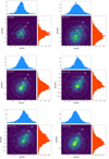 |
Fig. A.1. VPM, as 2D histogram diagram, of the stars in the cluster regions within the given radius r from its centre. Yellow areas are representative of over-densities, which become green and blue when the density decreases. White dot circles depict the 1σ, 2σ, and 3σ from the mean cluster PM value. On the top and on the right panels, we show the corresponding PM histograms, pmra (blue), and pmdec (red), respectively. We use a different bin size depending on the crowding of the areas. We add an insert for the VVV-CL160 cluster in order to make the PM over-density much more visible. |
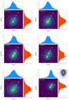 |
Fig. A.1. Continued. |
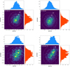 |
Fig. A.1. Continued. |
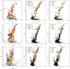 |
Fig. A.2. Left panel: VVV CMD for contaminated (grey points) and PM-decontaminated samples (Hess diagram). We show the position in the CMD of the RR Lyrae stars located at 12′ from the cluster centres (black squared) and those considered cluster members (magenta squared). Middle and Right panesl: 2MASS+VVV CMDs for PM-selected members. We fit a family of isochrones (cyan, red, and yellow lines), changing metallicities and ages, respectively. The red line is the PARSEC isochrones best-fit for each cluster (see Table 3). |
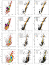 |
Fig. A.2. Continued. |
 |
Fig. A.2. Continued. |
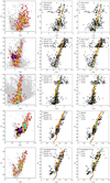 |
Fig. A.2. Continued. |
Appendix B: Additional Table
Properties of RR Lyrae samples in each GC field within 12′. We highlight with a star symbol all the variables that we consider members of the respective clusters.
All Tables
Position selection cuts for the PM-decontamination procedure, and mean cluster PMs for the GC candidates.
Main physical parameters for each star cluster candidate using the VVV photometry.
Optical parameters derived for those GCs for which it was possible to obtain adequate Gaia EDR3 data, which were used to confirm the VVV results.
Known and well-characterised GCs used to derive the total luminosity for each GC.
Properties of RR Lyrae samples in each GC field within 12′. We highlight with a star symbol all the variables that we consider members of the respective clusters.
All Figures
|
Fig. 1. VVV (on the left) and Gaia+VVV (in the middle) density maps for a r = 10′ field centred on VVV-CL150, which is used as a representative cluster. The redder areas are representative of over-densities, while the yellower areas are lower densities. The Gaia EDR3 + VVV CMD (on the right) is displayed for the same field. |
| In the text | |
|
Fig. 2. Map depicting Galactic latitude versus longitude for our sample. The confirmed GCs are highlighted as red points, whereas transparent red points are used to point out the unconfirmed GCs. We also mark with open red circles the open clusters excluded from our analysis. We show known GGs from Vasiliev & Baumgardt (2021) with open green squares for comparison. We use shorter cluster identifications only for our convenience. |
| In the text | |
|
Fig. 3. KDE technique applied to select the likely size of a cluster during the decontamination procedure. From left to right: scatterplot, 2D Histogram, Gaussian KDE, and 2D density with contours are shown for FSR 1767 (top panels) and VVV-CL160 (bottom panels) fields, which are used as representative. Green and yellow areas are illustrative of over-densities, while the blue areas show lower densities. |
| In the text | |
|
Fig. 4. Vector PMs shown to demonstrate that the kinematics of the star clusters analysed here are consistent with those of the known GCs located in the direction of the MW bulge. Our targets are highlighted with red points, whereas the known GCs located in the bulge within −10 < l(deg) < 10 and −10 < b(deg) < 10 are represented by open green squares. |
| In the text | |
|
Fig. 5. Spatial distribution for four clusters (on the top) and their relative fields (on the bottom) selected at 5′≲r ≲ 8′ from the cluster centre, taken as representative. We use the KDE technique, as in Fig. 3, in order to better distinguish the over-densities (yellow/green colours) from lower-densities (blue colours). (a) ESO 456-09, (b) VVV-CL131, (c) VVV-CL160, (d) VVV-CL150. |
| In the text | |
|
Fig. 6. Normalised PM histograms and CMDs for field (in red) and cluster (in blue) stars. We fit the Gaussian distributions (dashed lines) using means and standard deviations listed in Table 2. (a) FSR 0009, (b) FSR 1775, (c) FSR 1767, (d) VVV-CL110, (e) VVV-CL119, (f) VVV-CL128, (g) VVV-CL131, (h) VVV-CL143, (i) VVV-CL150 (j) VVV-CL153, (k) VVV-CL154, (l) VVV-CL160, (m) ESO 393-12, (n) ESO 456-09, (o) DB 044, (p) Kronberger 49. |
| In the text | |
|
Fig. 6. continued. |
| In the text | |
|
Fig. 7. Luminosity functions in Ks-band for each star cluster. Top: densogram used in order to more easily recognise the RC and avoid the binning dependence. The yellow colour depicts the highest density, with density decreasing towards magenta and then dark blue. We use a bin size of 0.1. |
| In the text | |
|
Fig. 8. De-reddened CMDs for field stars (on the left) located at 5′≲r ≲ 8′ from the FSR 1767 centre and for the FSR 1767 GC (on the right). We also construct the MKs luminosity function as blue histograms. |
| In the text | |
|
Fig. 9. Three-dimensional distribution of the star clusters analysed in this work towards the Galactic bulge using the Galactocentric coordinates (X, Y, Z). The red cross depicts the Galactic centre position at (0, 0, 0). The colour of points indicates the Galactocentric distance (RG in kpc) as specified by the legend. |
| In the text | |
|
Fig. 10. As Fig. 4, we show the star clusters tangential velocities to demonstrate that the kinematics of the star clusters analysed here are consistent with those of the known GCs from Vasiliev & Baumgardt (2021) located in the direction of the MW bulge. |
| In the text | |
|
Fig. 11. Gaia CMDs for the eight clusters for which we obtain reliable results in the optical passband. The black dotted line depicts the isochrone with the same age and metallicity as the VVV photometry and listed in Table 3. |
| In the text | |
|
Fig. 12. Spatial distribution of RR Lyrae variable stars detected within 12′ from GC centres. The magenta points represent the RR Lyrae that are considered cluster members. The distance error bars are of 0.5 kpc for each point. The dotted line depicts the heliocentric distance derived from the VVV photometry. |
| In the text | |
|
Fig. A.1. VPM, as 2D histogram diagram, of the stars in the cluster regions within the given radius r from its centre. Yellow areas are representative of over-densities, which become green and blue when the density decreases. White dot circles depict the 1σ, 2σ, and 3σ from the mean cluster PM value. On the top and on the right panels, we show the corresponding PM histograms, pmra (blue), and pmdec (red), respectively. We use a different bin size depending on the crowding of the areas. We add an insert for the VVV-CL160 cluster in order to make the PM over-density much more visible. |
| In the text | |
|
Fig. A.1. Continued. |
| In the text | |
|
Fig. A.1. Continued. |
| In the text | |
|
Fig. A.2. Left panel: VVV CMD for contaminated (grey points) and PM-decontaminated samples (Hess diagram). We show the position in the CMD of the RR Lyrae stars located at 12′ from the cluster centres (black squared) and those considered cluster members (magenta squared). Middle and Right panesl: 2MASS+VVV CMDs for PM-selected members. We fit a family of isochrones (cyan, red, and yellow lines), changing metallicities and ages, respectively. The red line is the PARSEC isochrones best-fit for each cluster (see Table 3). |
| In the text | |
|
Fig. A.2. Continued. |
| In the text | |
|
Fig. A.2. Continued. |
| In the text | |
|
Fig. A.2. Continued. |
| In the text | |
Current usage metrics show cumulative count of Article Views (full-text article views including HTML views, PDF and ePub downloads, according to the available data) and Abstracts Views on Vision4Press platform.
Data correspond to usage on the plateform after 2015. The current usage metrics is available 48-96 hours after online publication and is updated daily on week days.
Initial download of the metrics may take a while.