| Issue |
A&A
Volume 658, February 2022
|
|
|---|---|---|
| Article Number | A61 | |
| Number of page(s) | 34 | |
| Section | Stellar atmospheres | |
| DOI | https://doi.org/10.1051/0004-6361/202040116 | |
| Published online | 01 February 2022 | |
Upper mass-loss limits and clumping in the intermediate and outer wind regions of OB stars
1
Centro de Astrobiología, CSIC-INTA,
Ctra de Torrejón a Ajalvir km 4,
28850
Torrejón de Ardoz,
Madrid,
Spain
e-mail: mmrd@cab.inta-csic.es; m.m.rubiodiez@gmail.com
2
Facultad de Físicas, Universidad Autónoma de Madrid,
Campus Cantoblanco, Ctra Colmenar km 15,
28049
Madrid,
Spain
3
Instituut voor Sterrenkunde, KU Leuven,
Celestijnenlaan 200D,
3001
Leuven,
Belgium
4
IAPS-INAF,
via Fosso del Cavaliere, 100,
00133
Roma,
Italy
5
Universitäts-Sternwarte München,
Scheinerstr. 1,
81679
München,
Germany
6
European Space Astronomy Centre (ESAC)/ESA,
PO Box 78,
28690
Villanueva de la Cañada,
Madrid,
Spain
7
Center for Detectors, Rochester Institute of Technology,
Rochester,
New York
14623-5603,
USA
Received:
11
December
2020
Accepted:
22
June
2021
Context. Mass loss is a key parameter throughout the evolution of massive stars, and it determines the feedback with the surrounding interstellar medium. The presence of inhomogeinities in stellar winds (clumping) leads to severe discrepancies not only among different mass-loss rate diagnostics, but also between empirical estimates and theoretical predictions.
Aims. We aim to probe the radial clumping stratification of OB stars in the intermediate and outer wind regions (r ≳ 2 R*; radial distance to the photosphere) to derive upper limits for mass-loss rates and to compare that to current mass-loss implementation. Our sample includes 13 B supergiants, which is the largest sample of such objects in which clumping has been analysed so far.
Methods. Together with archival optical to radio observations, we obtained new far-infrared continuum observations for a sample of 25 OB stars. Our new data uniquely constrain the clumping properties of the intermediate wind region. By using density-squared diagnostics, we further derived the minimum radial stratification of the clumping factor through the stellar wind, fclmin (r), and the corresponding maximum mass-loss rate, Ṁmax, normalising clumping factors to the outermost wind region (fclfar = 1).
Results. We find that the clumping degree for r ≳ 2 R* decreases or stays constant with an increasing radius, regardless of the luminosity class or spectral type for 22 out of 25 sources in our sample. However, a dependence of the clumping degree on the luminosity class and spectral type at the intermediate region relative to the outer ones has been observed: O supergiants (OSGs) present, on average, a factor 2 larger clumping factors than B supergiants (BSGs). Interestingly, the clumping structure of roughly one-third of the OB supergiants in our sample is such that the maximum clumping occurs close to the wind base (r ≲ 2 R*), and then it decreases monotonically. This is in contrast to the more frequent case where the lowermost clumping increases towards a maximum and needs to be addressed by theoretical models. In addition, we find that the estimated Ṁmax for BSGs is at least one order of magnitude (before finally decreasing) lower than the values usually adopted by stellar evolution models, whereas the upper observational limits and predictions of OSGs agree within errors. This implies large reductions of mass-loss rates applied in evolution models for BSGs, independently of the actual clumping properties of these winds. However, hydrodynamical models of clumping suggest absolute clumping factors in the outermost radio-emitting wind of the order of fclfar ≈ 4–9, assuming these values would imply a reduction in mass-loss rates included in stellar evolution models by a factor 2–3 for OSGs (above Teff ~ 26 500 K) and by factors 6–200 for BSGs below the so-called first bi-stability jump (below Teff ~ 22 000 K). While such reductions agree well with new theoretical mass-loss calculations for OSGs, our empirical findings call for a thorough re-investigation of BSG mass-loss rates and their associated effects on stellar evolution.
Key words: radio continuum: stars / infrared: stars / stars: massive / stars: mass-loss / stars: early-type / stars: winds, outflows
© ESO 2022
1 Introduction
Wind outflows from OB supergiants are the most widely studied examples of the radiatively driven-wind physical phenomenon (e.g. Friend & Abbott 1986; Pauldrach et al. 1986; Puls et al. 1996). These radiation-driven winds were first described theoretically by Lucy & Solomon (1970) and Castor et al. (1975), hereafter CAK, assuming a stationary, homogeneous, and spherically symmetric outflow. By comparing observed spectral lines with expanding non-local thermodynamic equilibrium (NLTE) model atmospheres(e.g. CMFGEN, Hillier & Miller 1998; FASTWIND, Santolaya-Rey et al. 1997 and Puls et al. 2005; POWR, Gräfener et al. 2002)1, it is possible to derive both physical stellar and wind parameters by means of quantitative spectroscopy (e.g. Najarro 1995; Puls et al. 1996; Herrero et al. 2002; Urbaneja et al. 2003; Puls et al. 2005; Berlanas et al. 2018; Sander et al. 2014; Martins et al. 2019). However, despite the initial success of theoretical predictions based on stationary outflows (Vink et al. 2000; Kudritzki 2002; Puls et al. 2003), it is well established nowadays that stellar winds from massive stars are time-dependent and structured in velocity and density, displaying small-scale inhomogeneities (see review by Puls et al. 2008; Hamann et al. 2008; Sander 2017). These inhomogeneities change the structure of the atmosphere and wind, affecting the quantitative spectroscopic-based diagnostics used to obtain crucial stellar and wind parameters of massive stars.
Hydrodynamical wind simulations have shown that the presence of strong instabilities2 in the line-driven wind leads to formation of small-scale regions of very high densities (Owocki et al. 1988; Feldmeier 1995). These dense‘wind clumps’ can be described using either the fractional volume of dense gas, the volume filling factor (fv, Abbott et al. 1981), or via a clumping factor (fcl, Owocki et al. 1988):
 (1)
(1)
where ⟨ρ2⟩ and ⟨ρ⟩ are the mean of the squared density and the mean density, respectively, and where under the assumption of a negligible amount of gas in between the dense clumps in which one has  .
.
Time-dependent simulations further show that the clumping factor across the wind is not homogenous, but it presents radial stratification, fcl = fcl (r). Theoretical predictions agree on O supergiants (OSGs) in that the clumping structure first increases rapidly in the wind-acceleration region, and then it starts to fade again in regions far away from the star (Runacres & Owocki 2002, 2005). However, depending on the approximations and physical conditions used in the simulations (e.g. treatment of the source function, photospheric perturbations, or dimensionality), the onset of the clumping is predicted further away (Runacres & Owocki 2002; Dessart & Owocki 2003, 2005) or closer to the photosphere (Sundqvist et al. 2011, 2018; Sundqvist & Owocki 2013; Driessen et al. 2019), which can affect the formation of critical wind diagnostics as well as the spot where maximum clumping is achieved. The actual physical conditions close to the base wind (r ≲ 2 R*) represent an open challenge in line-driven wind theory.
It has been suggested than a turbulent photosphere (e.g. Cantiello et al. 2009) may be lead to the formation on clumps at the base of the wind. Of course, this process would affect the density structure of the wind quantitatively, at least close to the stellar photosphere. However, it is not clear how the influence of a turbulent photosphere could persist far out in the wind, and there are not theoretical simulations to probe. Therefore, for the purposes of this work, hydrodynamical LDI theory is used since it has been widely tested with success.
Since the presence of a density structure affects the matter-radiation interaction across the wind, a key consequence of wind-clumping regards its impact upon the effective opacity of the wind (see detailed overview in Sundqvist & Puls 2018). For processes scaling linearly with ρ, the mean opacity of the clumped medium is the same as for the homogeneous wind model, whereas for processes scaling with ρ2, the mean opacity is enhanced by a factor fcl. Empirically, this means that clumping differently affects the spectral diagnostic used to derive wind parameters. Assuming that all clumps are optically thin for a given mass-loss rate leaves unaltered diagnostic X-ray lines, electron-scattering wings, and scattering resonance lines (ρ-dependent; e.g. C IV, P V), whereas it causes an opacity enhancement of recombination lines or free-free continuum (ρ2 -dependent; e.g. Hα, Brγ, mid- and far-infrared, and radio continua). Therefore, if clumping is not appropriately taken into account, inconsistencies in mass-loss rate estimates between different diagnostics will arise (Fullerton et al. 2006; Cohen et al. 2010; Sundqvist et al. 2011). In particular, it is well established now that mass-loss rates of OB stars derived from the classical diagnostic Hα line are overestimated by a factor  if unclumped models are used in the analysis.
Moreover, if clumps become optically thick, this leads to additional light leakage through porous channels in between the clumps. Porosity can occur either spatially or in velocity space due to Doppler shifts in the rapidly accelerating wind. Studies of velocity-space porosity have shown that clumps do indeed become very easily optically thick in UV resonance lines and that this effect is critical to include when analysing such P-Cygni line formation (Oskinova et al. 2007; Hillier 2008; Sundqvist et al. 2010; Surlan et al. 2013). On the other hand, such velocity-space porosity does not affect the continuum diagnostics studied in this work. And as shown by Sundqvist & Puls (2018), under typical OB-star wind conditions, effects of spatial porosity upon the formation of mid- and far-infrared (MIR and FIR) and radio continua should be negligible. Nonetheless, these diagnostics are also subject to uncertainties related to wind inhomogeneities, in particular the level of clumping in the inner to intermediate (MIR and FIR region) and outermost (radio forming region) wind parts. These uncertainties, however, can be reduced by combining suitable diagnostics, effectively mapping the wind at different radial distances, from close to the base (V-band, Hα), over intermediate regions (Brα, MIR and FIR continua), to the outermost region (radio continuum). A consistent analysis here would place tight constraints on the radial clumping stratification. Moreover, if used in combination with ionisation and velocity law diagnostics (resonance lines; e.g. P V), orX-ray emission (Cohen et al. 2010), then absolute clumping factors and mass-loss rates could be uniquely derived.
First efforts have been performed by Puls et al. (2006) (hereafter, P06) and Najarro et al. (2008, 2011) by means of Hα, Brα, and IR-, millimetre-, as well as radio-continuum emission models for a sample of Galactic hot O stars. These studies show that whereas O giants seem to have similar clumping degrees throughout the wind, OSGs show, on average, a clumping facttor of about four times larger in the inner wind than in the outermost one. Thus, the mass-loss rate estimates for OSGs derived from Hα and smooth wind models should be scaled down by a minimum factor 2. The empirical clumping stratification derived by P06 and Najarro et al. (2011) suggested that the clumping degree starts to decrease at r ≈ 2–6 R*. This agrees rather well with the predicted clumping stratification overall at r ≲ 20 R* by hydrodynamics LDI simulations of OSGs (Sundqvist et al. 2011; Sundqvist & Owocki 2013; Driessen et al. 2019). However, due to the scarcity of reliable continuum observations of the analysed OB stars at FIR wavelengths, the clumping factor in the intermediate wind region (2 R* ≲r ≲ 15 R*) remains poorly constrained.
To investigate the radial clumping stratification of OB stars at r ≳ 2 R*, we obtained Herschel-PACS 70 and 100 μm fluxes (and the 160 μm flux for the brighter sources) for a carefully selected sample of OB stars. The sample consists of 25 OB Galactic supergiant, giant, and dwarf stars, covering spectral types from O3 to B3 - 4. Targets were selected to cover a wide OB-star parameter space, allowing us to analyse the behaviour of wind-clumping stratifications as a function of the luminosity class and spectral type. Moreover, the large number of OB supergiants in the sample allows for a deeper, statistically more significant analysis than previous work. In particular, our analysis represents a first attempt to derive the average properties of the clumping structure of B supergiants (BSGs) by means of a multi-wavelength analysis, carefully comparing them to the corresponding OSG results. In addition, the analysis allowed us to derive reliable upper limits to mass-loss rates, and to compare these with the existing mass-loss rate recipes (Vink et al. 2000, 2001, hereafter V00 and V01) usually used in evolutionary tracks.
This represents a unique opportunity to test (at least in a relative way) theoretical mass-loss predictions for BSGs across the so-called bi-stability jump. Since the quantitative mass-loss rates across this jump are critical for stellar evolution modelling (e.g. Vink et al. 2010; Keszthelyi et al. 2017), this has a rather important impact also on our general knowledge about the massive-starlife cycle.
The paper is organised as follows. Section 2 summarises the obtained Herschel-PACS observations and flux estimates of the sample, as well as the collected observations at different wavelengths from the literature. A description of the methodology, assumptions, and procedures can be found in Sect. 3, whereas the performed analyses and corresponding results are presented in Sect. 4. We discuss our findings in Sect. 5 and present conclusions and a summary in Sect. 6.
2 Observations and data reduction
Although the main goal of this work is to constrain maximum mass-loss rates and degrees of clumping in the intermediate wind region of OB supergiants, our initial 27 star sample also contains a few OB giants and dwarfs, including one LBV, two confirmed binaries, four early B-hypergiants (eBHGs) and one magnetic star (see Table 1). This sample allowed us not only to analyse clumping stratification by luminosity class and spectral type, but also to investigate clumping properties of some peculiar objects for the first time. Finally, although blue supergiant stars are known to display photometric and spectroscopic variability, suggested to be linked to stellar pulsations, our sample has been carefully selected to encompass blue supergiants in long stable stages (Clark et al. 2012), with the exception of HD 198478, an extreme case of spectroscopic variability3, with an important scatter in the stellar and wind parameters for this source (see Table A.1). Nonetheless, we included this star in the sample in order to further analyse the uncertainty in our estimated values due to the use of certain sets of stellar and wind parameters (see discussion Appendix A.2), and to account for the effect of possible strong variability not detected so far for the rest of stars in our sample.
In addition, we collected archival data in the literature for V-band, near-infrared (NIR), MIR, mm and radio fluxes, when available. In Table 1 we summarise the sample of stars observed with Herschel-PACS and the data collected for this work. The PACS column refers to our FIR flux observations. A description of the data reduction and the photometry processing of Herschel-PACS observations can be found in the following subsection, and the collected data are summarised in the successive sections.
2.1 FIR observations
FIR flux observations for our sample of 27 OB stars (Table 1) at 70 and 100 μm were taken with the Photodetector Array Camera and Spectrometer (PACS; Poglitsch et al. 2010) onboard theHerschel spacecraft (Pilbratt et al. 2010) in photometer mode (PI: Rubio-Díez, ID: OT1_mrubio_1, OT2_mrubio_2). A few of the objects in our sample have additional FIR-IRAS 60 and 100 μm data available, however most of them are upper limits (see references in Table 1).
Observations span from December 2011 to March 2013 and were done using the mini-scan map observing mode. In this mode, two scan maps are taken along the two array diagonal directions (110 and 70 degrees) at a constant speed of 20″ s−1 in parallel lines. The nominal spatial resolution for this scan velocity is 3.2″ pixel−1. Since our targets are point sources, a scan length of 2.5 arcmin was enough to cover the sky region of interest. The exposure times were estimated to reach a signal-to-noise ratio (S∕N) ≥ 10, using theoretical emission flux estimates. Additionally, PACS operates simultaneously in the two sidebands characteristic of heterodyne receivers. Thus, for each source in our sample a total of eight scans were obtained, two mini-scan maps at 70 and 100 μm (blue and green band), and four scans atextra band 160 μm (red band). The PACS point spread function (PSF) for these photometric bands have a full-width at half-maximum (FWHM) default value of 5.2″, 7.7″ and 12″, respectively.
The maps were processed using the map reconstruction task PhotProject with the Multi-resolution median transform (MMT) deglitching method implemented in HIPE (Herschel Interactive Processing Environment, Ott 2010). A second deglitching grade was applied.Subsequently, the processed mini-scan maps were combined into a final map (Fig. 1). We observed that whereas for the faint sources a second deglitching does not make major changes in the final maps, for our brightest sources this step improved the accuracy of the recovered fluxes. Therefore, for the photometry in our sample stars we decided to use the second deglitching processed maps. Since the observing strategy focused on flux observations at the blue and green bands, the quality of the final extra red maps are generally poor and just a few sources have been detected at this band, most of them giving upper limits. Table 2 displays the observed sources and the bands where they were detected. Only two sources of the initial sample have not been detected or reliably detected, HD 190603 and CygOB2#7,respectively. Thus, our final sample is conformed of a total of 25 OB stars (Tables 3 and 5).
Herschel/PACS Photometry
To perform the point source aperture photometry we used Hyper (Traficante et al. 2015). This routine was initially designed for FIR point source photometry in complex sky regions in the framework of the Herschel infrared survey of the Galactic plane (Hi-Gal). Because of its modularity and versatility, this code can be easily adapted to our Herschel-PACS observations, and it has been successfully used by different authors already (e.g. Benedettini et al. 2015; Svoboda et al. 2016; Li et al. 2018; Paulson & Pandian 2020).
Hyper combines 2D multi-Gaussian fitting with aperture photometry to provide reliable photometry in regions with variable background,and in crowded fields. The 2D Gaussian fitting takes into account the beam observations and the source elongation to estimate theregion over which to integrate the source flux, that is it computes the PSF of the source onto the final map. The background was locally evaluated and removed for each source using polynomial fits of various orders. The code selected the background based on the lowest r.m.s of the individual residual maps. For most of the sources, a polynomial with order not larger than 2 was used. In addition, in the case of blended sources, Hyper would perform a simultaneous multi-Gaussian fit of the main source and its companion(s), subtracting the modelled companion(s) from the science target. This was nothe case for any of our targets. Finally, although this code allows simultaneous multi-wavelength photometry,we performed a careful and individual aperture photometry for each source, by defining a map-region around the sources of interest. This allowed to optimise the 2D-Gaussian fitting procedure for the faintest sources, as well as flux estimations. Moreover, for those maps where the background varies significantly along the whole field of view, this enables a proper detection of the target, even in the case where only upper flux limits were estimated.
The final fluxes of the OB stars at the blue, green, and red bands were obtained applying the aperture and colour corrections to the extracted fluxes of the sources. We estimated the uncertainty in the measurements as well as the S/N of the detection.
The error in the estimated final flux includes the uncertainty in the maps calibration from PACS (10%), the error from the photometric procedure (from Hyper outputs) and from the aperture and colour corrections applied to the extracted flux. These corrections are needed to (i) account for the missing flux due to the finite aperture; and (ii) convert monochromatic flux densities in the PACS data products, which refer to a constant energy spectrum, to the true object Spectral Energy Density (SED) flux densities at the reference band wavelengths 70, 100 and 160 μm, using the tabulated aperture and colour correction factors to the extracted PACS flux as 1/fapcfcc4.
Finally, attending to the S/N we flagged flux values with quality flags (qFλ) as: ‘A’ for detections with S∕N ≥ 10, and ‘B’ for detections with 5 ≤S∕N < 10. In addition, measured fluxes with S∕N ≤ 5 or affected by image artefacts, are flagged as upper limits (U). In Table 2 we summarise the obtained flux values and the corresponding errors at 70, 100 and 160 μm of the sample.
List of the OB stars observed with Herschel-PACS (IP: OT1_mrubio_1/OT2_mrubio_2) and the photometric data compiled from the literature used in this work (see references below).
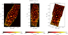 |
Fig. 1 From left to right: PACS 70 μm miniscan maps taken at position angles 70° and 110°, and the final composed image of the O supergiant star HD 66811 (ζ Pup). |
Herschel/PACS 70, 100, and 160 μm fluxes for our sample stars.
2.2 V/NIR and MIR observations
The V, NIR and MIR magnitudes used in this work are listed in Table 1 and were mostly collected from the literature (see references within). All sources are observed in the V and NIR bands, most of them also at MIR wavelengths. Since these observations were made with different instruments (different photometric systems) we performed an absolute flux calibration. We used Vega as a calibrator to convert the magnitudes into absolute fluxes by extrapolating the visual absolute flux calibration of Vega to a specific wavelength by model atmosphere (Kurucz models) and calculating the absolute fluxes of Vega in the differentphotometric systems. A detailed description of the absolute flux calibration procedure can be found in Puls et al. (2006).
2.3 Millimetre and radio observations
Millimetre and radio observations were collected from literature (see Table 1 and references therein). Most of our sample starswere observed with the Very Large Array (VLA) at 2, 3.5 and 6 cm or with the Australia Telescope Compact Array (ATCA) at 3.6 and 6 cm in different epochs. In addition, several objects were also observed at 1, 3, 13, 20 and 90 cm (J-VLA) and at 21 cm (e-MERLIN). Only for one object, HD 53138, no radio observations are available, whereas for 7 of the 25 targets only upper limits could be obtained.
With respect to the sub-mm and mm flux continuum measurements, we collected from the literature those obtained at 0.7, 0.85, 1.3 and 1.35 mm, when available. Only 7 stars in our sample have millimetre observations (Submillimetre Common-User Bolometer Array, SCUBA).
2.4 Gaia distances
This work uses distance determinations based on Gaia DR2 parallaxes (Luri et al. 2018; Gaia Collaboration 2016, 2018). We only used parallaxes where the associated errors are lower or similar to 15% (8 out of 25 objects; marked with an asterisk in Table 3), otherwise the obtained distance becomes unreliable when compared to previous estimates (see below). The differences between Gaia DR2 and older distance estimates range from 0.01 kpc to ≈ 1 kpc, with an average of 0.47 kpc. The largest deviations correspond to HD 169454, HD 80077, and Cyg OB2#12, whose differences with the new values are ~0.6, 1.05, and 0.9 kpc, respectively.
In particular, for Cyg OB2#12 the distance derived from Gaia DR2 parallaxes (0.85 kpc) puts the star much closer than its association, Cygnus OB2 (1.75 kpc). This casts some doubts about its physical properties (Nazé et al. 2019). For this source we provide the results of the analysis for both distances (two entries in Tables 6, 7 and 9), although only the result pertaining to the larger, association distance (1.75 kpc) is considered in the discussion5.
The case of HD 80077 is different. Since there were always severe doubts about this star being a member of the Pismis 11 cluster (located at 3.6 kpc; Marco & Negueruela 2009), and given the lower uncertainty in the parallaxes by Gaia DR2, we keep this distance (2.55 kpc) for the analysis.
For the rest of the sample, initially we used photometric distances from the literature (see Tables 3 and 5), whose uncertainties range between 0.1 and 0.4 kpc6, and locate most of the stars in their associated cluster. For HD 152236 (τ1 Sco) we assumed a distance of 1.64 kpc (Sana et al. 2006), used in previous studies (Clark et al. 2012).
In Table 3 we present the final used distances and the derived stellar radii and extinction parameters for the sample as described in Sect. 3. For HD 66811 (ζ Pup), in order to be consistent with previous analyses by P06 (see Table 5), we used two different distances: a commonly used shorter distance (0.46 kpc), assuming ζ Pup is part of Vela OB2 association, and a larger one (0.73 kpc, Sahu & Blaauw 1993), which corresponds to the star being runaway. Although we provide the results of the analysis for both distances (two entries in Tables 6, 7 and 9), the discussion in this work refers to the shorter distance, unless otherwise specified.
Final used distances and associated errors, reddening parameters and derived stellar radii.
3 Modelling
To investigate the wind clumping stratification and mass-loss rates of the 25 OB stars in our final sample, we modelled their observed spectral energy distribution (SED) from V/NIR to radio wavelengths. We used the interactive procedure developed by P06, which is based on continuum emission models (photospheric plus wind emission), assuming a spherically symmetric wind calibrated against full NLTE stellar atmosphere models, and accounting for optically thin clumping. Although the basic method thus neglects potential effects from porosity (see Sect. 1), these should be relatively small for the diagnostics and spectral ranges considered in this work (see Sundqvist & Puls 2018 for a discussion). Below we present a summary of the approach to model SEDs depending on the stellar and wind parameters of the objects. An in-depth description and verification of the method can be found in P06.
3.1 Infrared and radio flux emission
The infrared and radio fluxes are calculated using the approximations described by P06, based on Lamers & Waters (1984) and the following parametrization.
The Wind velocity law is including as
 (2)
(2)
with  and the minimum velocity, υmin, set to 10 km s−1.
Electron temperature
The electron temperature was computed using Lucy’s temperature law (Lucy 1971) with a lower temperature cut-off at 0.5 Teff.
Ionisation equilibrium
For all the objects in our sample, hydrogen is considered to be completely ionised, whereas the helium ionisation structure used in the modelling of the SED depends on the temperature of the source and the wavelength domain (for the rationale see P06). Specifically, for the majority of the sample (17 000 K ≲Teff ≲ 35 000 K) helium is considered singly ionised in the radio regime whereas for the coolest (Teff ≲ 17 000 K) and hotter objects (Teff ≳ 35 000 K), it is assumed to be neutral and fully ionised, respectively. In the NIR, helium is assumed to be fully (Teff ≳ 32 500 K) or singly (13 000 K ≲Teff ≲ 32 000 K) ionised. A particular treatment is required for P Cyg (HD 193237) whose ionised helium structures depart from the above standard scalings with effective temperature (Najarro & Figer 1998). As such, for P Cyg we assumed that helium is fully recombined in the outer parts of the wind (radio domain) and singly ionised in the inner ones (NIR domain).
Photospheric input fluxes
For λ < 1μm, where the stellar photosphere dominates, the emitted flux is modelled using Kurucz’s fluxes. On the other hand, for λ > 1μm, where the wind starts to dominate the resulting flux, a black body emission model is used.
Wind clumping treatment
Clumping is included using the following approach: all material in the wind is redistributed into clumps which are over-dense with respect to the average density, we assume optically thin clumps (see above), and further that the inter-clump medium is effectively void (Abbott et al. 1981; Schmutz 1995).
Under these assumptions, the spatial mean density (⟨ρ⟩ = Ṁ∕4πr2υ) and mean squared density can be expressed as a function of the volume filling factor (fv) as:
 (3)
(3)
 (4)
(4)
where ρ+ denotes the density inside the clump. Thus, the clumping factor (fcl) as describedby Eq. (1),
 (5)
(5)
 (6)
(6)
becomes the inverse of the volume filling factor, describing the over-density of the clumps as compared to the mean density.
Within this approach, the opacity depends only on the matter and the physical processes inside the clumps (recombination, scattering, absorption, etc.). Since the mean opacity of the processes with opacities depending on ρ2 is enhanced by a factor fcl (see Sect. 1), the optical depth invariant for thermal emission, Q′ (Lamers & Waters 1984; P06), is modified as:
 (7)
(7)
Therefore, since the opacities of all processes considered in this analysis depend on ρ2 (IR/mm/radio emission), the effects of clumping can be included in the models by multiplying the opacities evaluated for the mean wind by a clumping factor. Thus, the theoretical-emitted flux (Panagia & Felli 1975; Wright & Barlow 1975),
 (8)
(8)
for such processes might be extended according to:
 (9)
(9)
Consequently, the emitted flux is sensitive to changes in clumping factors, allowing us to constrain the clumping structure of the wind by fitting emission models to flux observations for a given source. Since clumping is not constant throughout the wind but presents a radial stratification, fcl (r/R*), it is to be evaluated in different regions of the wind.
For that objective, the wind is divided in different regions with corresponding clumping factors as defined in Table 4. Typical boundaries are rin = 1.05 R*, rmid = 2 R*, rout = 15 R* and rfar > 50 R*, which roughly agree to the formation zones of Hα and NIR (Region 1 – 2), MIR/FIR (Region 3), mm (Region 4) and radio (Region 5). We note that (i) the clumping at the base of the stellar wind (1 <r/R* <rin) is set to 1 within the fitting procedure, and (ii) that the above-mentioned limits for the wind regions in Table 4 can be adapted within the fitting procedure when necessary (see below). Figure 2 displays a sketch of the defined wind regions as a function of the spectral energy distribution.
The parametrisation adopted in this work is designed to empirically constrain the clumping factor in different radial wind zones. Therefore, the derived clumping factors should be considered as average values describing the global behaviour of clumping throughout the wind. Since all used diagnostics depend on ρ2, it is not possible to derive absolute values for clumping factors and mass-loss rates, but only relative ones. What we really obtain is the scaling invariant  for a given radius interval. To derive absolute values, a simultaneous analysis of ρ-dependent diagnostics (e.g. resonance lines, see Sect. 1) would be required to break the degeneracy, which is out of the scope of this work. However, since all derived (minimum) clumping factors and (maximum) mass-loss rates can be scaled via Q′, it is still possibleto carry out important comparisons with theoretical predictions as well as with previously derived empirical values.
It is worth noting that our fitting-results are independent of the individual values for distance and stellar radius, and that they can be easily scaled to different values as long as Q’ and (R*/d) remain conserved (see Eq. (9)). Of course, changes in distances (and thus in stellar radius) affect directly the derived absolute values of mass-loss rates, but it does not affect the behaviour of the clumping structure (e.g. HD 66811 and Cyg OB2#12, see Table 6).
All comparisons with other empirical studies and theoretical predictions were performed for the same values of distance and stellar radius, for a given source. Thus, for comparisons with other empirical studies, their mass-loss rates were scaled to the distance and stellar radius used in our analysis, whenever necessary. Similarly, stellar parameters used to compute theoretical predictions for Ṁ (Sect. 5.1.2) are the same as those used to derive the empirical Ṁmax estimates. Regardless of variations in absolute values of mass-loss rates with changing distance to the objects, the general behaviour found in this work will thus be unaffected, and the ratio between empirical and theoretical mass-loss rates is remains conserved. For example, we estimate that a 40% increase in distance7 leads to a decrease in empirical to theoretical mass-loss rates of around 30%. In other words, such changes in distance would not change the overarching trends and conclusions found in this work.
Defined wind region boundaries and the corresponding clumping factors used in this work.
 |
Fig. 2 Schematic of the wind emission: different wind regions as a function of the spectral range and their corresponding radial distance to the photosphere (r), as defined in Table 4. The emission model corresponds to the unclumped stellar wind of a O supergiant star (Teff = 33 kK, Ṁ = 8.6 × 10⁻⁶ M⊙ yr−1). |
3.2 Fitting procedure
We compare continuum emission models with the observed SED for the 25 OB stars in the sample. In Table 5 we summarise the stellar and wind parameters of the sample from the literature (references therein), used as input values in our simulations. The best-fit model for each source is obtained from a simple maximum likelihood method (χ2) as follows:
First, we de-reddened the observed flux using the extinction law provided by Cardelli et al. (1989). By comparing the observed V JHK fluxes with theoretical flux emission predictions we derived values for the colour excesses E(B − V) and their corresponding RV.
Secondly, we computed the stellar radius. For a given distance, the initial value of the stellar radius is adapted to match the V JHK de-reddened observed fluxes. Since flux is diluted by (R*/d)2 (see Eq. (9)), the ratio between radius and distance represents a scaled flux factor, which has to be conserved for any distance. In Table 3 we present the final used distances, and the corresponding derived stellar radiii and de-reddening parameters.
Thirdly, we estimated mass-loss rates required to reproduce the continuum distribution across the electromagnetic spectrum. Since the optical depth and the diluted flux scale with Ṁ/R*3∕2, this ratio has to be conserved for a given (R*/d).
Initially, all clumping factors in our simulations are set to the minimum value,  =
=  =
=  =
=  =
=  = 1 (unclumped wind), and the mass-loss rate is adapted to reproduce the observed fluxes throughout the wind (1.05 R* < r < 100 R*). Note that the emitted flux decreases on average with increasing wavelength and, therefore, radio thermal emission represents the lowest absolute flux values for a certain source8. As such, the derived Ṁ represents the maximum possible mass-loss rate (Ṁmax) consistent with radio observations assuming a minimum clumping condition (
 =
=  = 1). In the cases where radio fluxes are well-defined but somehow larger than at shorter wavelengths, the estimated Ṁmax relies instead on the consistent observed fluxes at those wavelengths (usually the FIR domain). The same is true for those sources whose radio observations are not well constrained, although in this cases the adopted Ṁmax is only an upper limit.
Finally, the radial stratification of the clumping is derived by adapting the values of the clumping factors to match the continuum emission. The best-fit solution for each source corresponds to the emission model (Ṁmax, R*, d and  ,
,  ,
,  ,
,  ) providing the minimum value of the statistics fitting function χ2. Unlike P06, we follow two different approaches: (i) Fixed-regions approach. Here, we fix the defined radial boundaries (see Table 4) for all sources. This allows us to investigate consistently the global behaviour of the clumping stratification for our sample, comparing the derived average clumping factors across the wind regions. (ii) Adapted-regions approach. In these simulations, the limits of the wind regions can be adapted, in addition to the clumping factors – when necessary – to secure the best possible fit compared to fixed-region approach. This allows us to probe also the boundaries defined above for the different wind regions.
Sample of analysed OB stars in this work and the initial set of stellar and wind parameters from the literature (‘ref’ column) used as input values in our simulations. log g indicates gravities without centrifugal correction.
3.3 Additional considerations
In order to be consistent, besides setting rout = 15 R* in the fixed-regions approach in our simulations, we also probe rout = 10 R*, since this limit was used by P06 when analyzing low or intermediate density winds (where, in their case, the profile shape of Hα served as a proxy for wind-strength).
Additionally, due to the relative scarcity of observations in the sub-mm regime, we computed the maximum clumping values for Region 4 still compatible with flux emission at shorter and longer wavelengths ( in Tables 6 and 7). For the sources previously analysed by P06, and with new distance estimates from Gaia (asterisked values in Table 3), we first tested the derived Ṁmax and clumping stratification by these authors against the obtained FIR flux values and the additional measured fluxes at MIR and radio rangesfound in the literature since P06. In a second step, we scaled the stellar radius and the mass-loss rate to the new distance according to Eq. (8) and derived the best-fit solution to all data as described above.
3.4 Prototypical examples
In this section we briefly describe three prototypical examples of the Ṁmax and clumping factor estimates through the fitting procedures in the fixed-region approach. They cover different possibilities with respect to the flux values, and how arising peculiarities are reflected in the table entries displaying the results for the whole sample (Tables 6, 7, 9). From top to bottom Fig. 3 displays observed and synthetised fluxes for HD 151804, HD 193237 (P Cyg), and HD 24398 (ζ Per). For a detailed discussion of every star in the sample, see Appendix A.
HD 151804
This is one of the most straightforward cases, where the radio flux is a unique, determined value providing a well constrained Ṁmax. For Ṁmax = 6.4 × 10⁻⁶ M⊙ yr−1, the synthesised flux perfectly matches the observed values across the wind without the need for clumping ( =
=  =
=  = 1), except in the intermediate wind region (Region 3). The synthesized fluxes with all clumping factors set to unity are displayed as a magenta-dotted line. To reproduce the observed fluxes in the FIR, we increase to
  = 3.2 (best-fit, solid line). Although the best-fit for this star has
  = 1, given the observational gap in the mm-regime a maximum value of the clumping degree in Region 4
  = 8 (blue dashed-line) is still consistent with the data at shorter wavelengths. This
  is typed between parentheses in the corresponding entry for this star in Table 6.
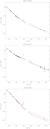 |
Fig. 3 From top to bottom: observed and best-fit fluxes vs. wavelength in the fixed-regions approach for HD 151804, HD 193237 (P Cyg), and HD 24398 (ζ Per). Solid lines correspond to the best-fits; magenta-dotted, blue-dashed and orange-dashed-dotted lines correspond to different models (see text). |
HD 193237 (P Cyg)
This known LBV is well sampled throughout the wind. It is well established that the observed variability on timescales of the order of months at millimetre and radio wavelengths (Abbott et al. 1981; van den Oord et al. 1985; Bieging et al. 1989; Scuderi et al. 1998; Ofek & Frail 2011; Perrott et al. 2015) is not related to P Cyg being a non-thermal source, but rather to changes in the ionisation stage of the outer wind (recombined outermost wind model, Najarro et al. 1997; see also Pauldrach & Puls 1990). In addition, the observed larger IRAS and SCUBA flux measurements at 60 and 850 μm may be due to spatial resolution effects (such as contamination by the characteristic LBV nebula surrounding P Cyg), whereas the lower value at 6 cm observed by Bieging et al. (1989) has not been confirmed by newer measurements. In view of this, we estimated Ṁmax for P Cyg for being consistent with all measured fluxes from 2 to 21 cm, regardless of the upper IRAS 60 μm and SCUBA 850 μm values and the lower flux at 6 cm, obtaining Ṁmax = 12.8 × 10⁻⁶ M⊙ yr−1.
With this mass-loss rate the synthesised flux underestimates the data at shorter wavelengths (magenta-dotted line). Thus, the clumping degree needed to be increased to reproduce the observed SED, yielding  = 3,
= 3,  = 3.5,
  = 5 and
  = 1 (best-fit, solid line). To match the larger well-defined fluxes observed in the radio-regime the clumping degree in Region 5 had to be increased to
  = 1.5 (blue-dashed line). The corresponding clumping factors for these two models for
  are separated by a forward slash (/) in Table 6, with the number on the left referring to the best-fit solution. The well-sampled mm-regime of this star further allows us to constrain the clumping degree in Region 4 to
  =
=  = 5.
= 5.
HD 24398 (ζ Per)
Only an upper limit of the flux at radio wavelengths is available for this star. An estimate of Ṁmax by matching this limit is not consistent with FIR flux values, since any model with such Ṁmax would overestimate the FIR flux (magenta-dotted line). Instead, an upper limit Ṁmax ≲ 0.18 M⊙ yr−1 derived from the FIR flux values is consistent with the radio upper flux limit. In this case the observed SED is perfectly matched by the minimum clumping degree throughout the whole wind,  =
=  =
=  =
=  = 1 (best-fit, solid black line). It is possible, however, to still match the upper radio flux limit if increasing up to
  = 5 (parenthesed value in Table 6; blue-dashed line). Although the best-fit for this star is for
  = 1, given the observational gap at λ > 100 μm,
  = 45 (orange-dashed-dotted line) is still consistent with the data (also between parentheses in Table 6).
4 Analysis and results
In this section we present the derived maximum mass-loss rates, the corresponding minimum radial clumping stratification, and their associated uncertainties.
The results obtained in the fixed- and the adapted-regions approaches (see previous section) are summarised in Tables 6 and 7. A detailed description of the fits for the individual objects can be found in Appendix A.
4.1 General findings
Overall, we find that the minimum χ2 of the fits inthe fixed-regions approach is comparable to that obtained with the adapted-regions approach. As such, unless specified otherwise, the following general findings refer to the best-fit solutions in the fixed-regions approach (Table 6). A definite Ṁmax was derived for 17 of the 25 sources. For the remaining 8 objects, we only provide upper limits of Ṁmax consistent with the observations, due to lack of detections in the radio regime.
Figure 4 displays log Q′ = log (Ṁmax/R*1.5) as a function of spectral type and luminosity class. We can see that log Q′ decreases with luminosity class and spectral type, and that the values departing from this trend correspond to the non-standard sources in our sample, i.e. confirmed binaries, magnetic stars, LBVs and eBHGs (see coloured symbols in Fig. 4). In particular, this figure shows that non-standard OB stars seem to be displaced towards higher log Q′ values and later spectral types when compared tostandard OB supergiants9.
Due to the low number of OB giants and dwarfs in our sample, it is not possible to clearly observe a similar behaviour as that seen for the OB supergiants. Overall, the general trend and the estimated values of Ṁmax and log Q′ for the complete sample appear consistent. Indeed, the large values obtained for some of the non-standard objects agree with some previous estimates (Clark et al. 2012; Crowther et al. 2006). For instance, for the eBHG star HD 152236, we derived Ṁmax = 6.2 × 10⁻⁶ M⊙ yr−1, a value close to the (unclumped) mass-loss rates obtained by these authors, 6.33 × 10⁻⁶ M⊙ yr−1 and 6.0 × 10⁻⁶ M⊙ yr−1, respectively.
The derived minimum clumping structures derived for r ≳ 2 R* are displayed in Table 6. Only one source, Cyg OB2#11, remains unconstrained in the intermediate wind region ( ≲ 3) since only upper flux limits were detected at 70, 100 and 160 μm. In Fig. 5 we present the ratio of the clumping factors in the intermediate and outer part of the wind (
 /
/ ; left panels) and in the intermediate and outermost wind regions (
 /
/ ; right panels)as a function of the wind density (log Q′), for the OB supergiants (top and middle panels, respectively) and for the OB giants and dwarfs (bottom panels). From top to bottom, Fig. 5 shows that the clumping degree decreases or remains nearly constant with increasing radius throughout the wind regardless of luminosity class or wind density. Overall, the minimum clumping degree in Region 4 (
 ) is similar to that in the outermost Region 5 (
 ). OB giants and dwarfs are the sources with generally the lowest, most homogeneous clumping across all wind regions. OB supergiants, on the other hand, display a more radially structured clumped wind.
There are four exceptions to these general trends, where the clumping structure seems to increase with increasing distance to the photosphere. These are P Cyg (HD 193237), Cyg OB2#12, ι Ori (HD 37043) and τ Sco (HD 149438). Note that all these are non-standard objects: respectively, a LBV, an eBHG with a recently measured variable radio flux at 21 cm (Morford et al. 2016), a confirmed binary, and the well-known magnetic B Dwarf τ Sco.
Maximum mass-loss rates, minimum clumping factors and alternative boundaries of the defined wind regions (adapted-regions approach, see Sect. 3) providing the best-fit models for some objects in the sample.
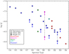 |
Fig. 4 Derived invariant log Q′ = log (Ṁmax/R*1.5) for our sample as a function of spectral type, in units of M⊙ yr−1 R⊙−1.5. Different symbols and colours represent the luminosity class coverage in the sample and the nature of the sources, respectively. Arrows indicate objects with upper limits for Ṁmax, and symbols joined by dashed-lines correspond to sources with two possible solutions for Ṁmax. |
4.2 Clumping in the intermediate wind of OB supergiants
The relatively large number of OB supergiants in the sample allows for a statistically significant analysis of the average radial clumping structure of these stars at r ≳ 2 R*. To do this, we use the fixed-regions approach and remove from the analysis those OB supergiants with a peculiar nature and/or whose derived clumping properties significantly depart from the general trend (HD 193237, Cyg 0B2#12, HD 149404, HD 198478; see Table 6). Due to the large uncertainty in PACS flux estimates for HD 194279 at 70 and 100 μm, the scarcity of data at mm wavelengths and the lack of evidence of it being a non-thermal emitter, we consider the first derived solution to be more likely for this target (first entry in Table 6; for discussion see Appendix A.2).
Figure 6 displays the individual (top panels) and the average (bottom panels) minimum radial clumping stratification for the OSG and BSG sub-samples (left and right, respectively). The OB supergiants show a similar or larger clumping degree in the intermediate wind region than in the outermost ones (Regions 4 and 5). We estimate that for OSGs the average minimum clumping factor for the intermediate wind region is ⟨ ⟩ ~ 4.0 ± 1.5, whereas for BSGs it is ⟨
 ⟩ ~ 2.1 ± 1.1 (errors represent standard deviations).
Concerning the outermost wind regions, due to the scarcity of sub-mm and mm observations it is possible to derive precise clumping properties in Region 4 for only 7 sources (boldfaced names in Tables 6 and 7). For the rest of the objects,  = 1 generally provides the best-fit solution, but larger values may also be possible (see
  Col. in Table 6). We compute an average minimum clumping factor for OSGs and BSGs of ⟨
  ⟩ = 1 (+2) and 1 (+1.3), respectively.Unlike for ⟨
  ⟩, the number in parentheses here do not represent formal errors, but are instead rough indications based on the average ratio ⟨
  ⟩ of those 7 OB supergiants whose clumping properties are fully constrained.
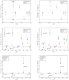 |
Fig. 5 From top to bottom: clumping factor ratio |


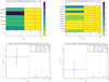 |
Fig. 6 Top: individual minimum and average values of the clumping factors for r ≥ 2 R* derived in the fixed-regions approach for the sub-sample of O (left) and B (right) supergiants (see Sect. 4.2). Bottom: average minimum clumping stratification of the sub-sample as in the top panel, with error bars. Solid error bars correspond to the standard deviation of ⟨
|


4.3 Clumping factor uncertainties
The mass-loss rate and clumping factor derivations have been made using literature-values of β and υ∞. As discussed above, the synthesized and observed fluxes depend mostly on the local quantities Ṁ  (for a given R*). Assuming an (almost) perfect fit, the derived clumping factors scale inversely with the mass-loss rate as δfcl ∕fcl ≈−2 δṀ∕Ṁ. Taking into account that uncertainties in Ṁmax depend directly on the errors in radio fluxes (temporal variability and/or intrinsic errors) with 2 δṀ∕Ṁ ≈ 1.5 δFν∕Fν, it follows that the uncertainty in clumping factors also scales inversely with flux as δfcl ∕fcl ≈−1.5 δFν∕Fν. We computed an average uncertainty ~15% for Ṁmax due to flux uncertainties, which leads to an average uncertainty in derived clumping factors of ≈30%. For those sources with uncertainties in Ṁmax above average, the errors in the clumping factors can reach 50%.
Other factors affecting the derived Ṁmax, and thus fcl, are the assumed helium fraction and the ionisation stage. We performed several simulations varying both parameters. We found that a factor 2 difference in the helium fraction leads to a variation in Ṁmax of ~16%, quite similar to the uncertainty found (~15%) when the ionisation state in the region probed in the mm and radio domain is different than assumed. From these simulations, we estimate that the average uncertainty of the clumping factors derived in this work, due to uncertainties in Ṁmax, is in between 30 and 40%.
4.4 Clumping dependence on β
Whereas the clumping degree in the outermost wind regions (r ≳ 15 R*) does not depend on the exponent of the velocity field, β, the opposite is true for the inner wind (r ≲ 2 R*). Since the β and υ∞ used in our analysis come from a range of different studies (see references in Table 5), they are not really coherently derived. Thus, some analysis regarding the impact of β on the derived clumping factors is warranted, and carried out below using two experiments. In the first one, we computed the boundaries of the validity interval of β for which a given best-fit model still reproduced the data with a goodness of fit within 10% of the corresponding minimum χ2. The resulting β-intervals are presented in Table 8 as
 (10)
(10)
with β0 being the used β in our simulations. We found that the limits of the intervals are not symmetric with respect to the used β (except in four objects). Moreover, our best-fit solutions are less sensitive to a decrease than to an increase of β, regardless of luminosity class, spectral type or ‘nature’ of the source (Fig. 7). Thus, our best-fit solutions are valid for average changes of β of ⟨ |δβ−∕β0| ⟩≈ 24% and ⟨ |δβ+∕β0| ⟩≈ 16%.
In the second experiment we computed new fitting models. We varied the clumping factors (and Ṁmax, if necessary) for different values of β, until a best-fit solution was found. This test estimates the errors of the derived clumping factors as:
 (11)
(11)
with δβ′ = β′− β0. In Table 9 we present the results of these simulations for fcl (β′), with β′ = (β1, β2), where β1 ≾ β−, β2 ≿ β+, and β0 is the used β in our simulations.
Note that for some sources the values of the alternative β1 and β2 are larger (or lower) than the typical limits derived from spectral line fitting (though always consistent with the theoretical limit β > 0.5). Nonetheless, our approach allows us to check the validity of the analysis as a function of β. From this experiment we found that, as expected, (i) large clumping factors,  , correspond to low values of β′ and vice versa, i.e. δfcl ∝−δβ′; (ii) changes in β do not uniformly (or symmetrically) affect all the defined clumping factors, and also depend on luminosity class. Thus, for OB supergiants, average values
  15–30% lead to average uncertainties of about 15–60% in
  and ~15% in
  . On the other hand, for the sources with weaker winds in our sample, i.e OB giants and dwarfs, average values of
  15–40% translate into average uncertainties of about 10–15% for
  , and up to 8% for
  ; and (iii) for a few sources, an increase of β cannot be compensated by a decrease of clumping factors, since the clumping factors for the used β reach unity, so that instead a decrease in Ṁmax is required (last column in Table 9).
Note that the objects with weaker winds and upper limits in Ṁmax also require a clumping increase in the outermost wind region,  (fclmax) > 1, in order to be able to consistently reproduce upper radio-flux limits. Our results agree with the average uncertainties estimated for
  and
and  by P06 (~30 and ~20%, respectively) by means of Hα profiles and IR/radio fluxes analyses in parallel.
Considering these experiments, the average error due to β uncertainties for the estimated values of  is ~30%, even in the extreme case that the actual values of the wind acceleration parameter β would be significantly different from those adopted in this work.
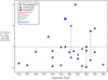 |
Fig. 7 Absolute ratio between the semi-widths (δβ+, δβ−) of the validity interval of β as a function of spectral type for the best-fit solutions derived in the fixed-regions approach in this work (see Table 6). Symbols and colours as in Fig. 4. The circled symbol indicates that the ratio was divided by 3 for display purposes. |
5 Discussion
The previous section showed that the clumping structure can be well described relative to the outermost wind in Region 5 (radio domain). Assuming for now minimum values  =
=  = 1, this allows us to discuss in detail the relative radial clumping-behaviour as well as the derived upper limits Ṁmax.
5.1 Clumping properties of OB stars
5.1.1 Radial stratification at r ≳ 2 R*
A key finding of our analysis is that clumping at r ≳ 2 R* presents similar radial stratification regardless of the strength of the wind, always fullfilling the condition  ≳
≳ 

 (see Tables 6 and 7).
The specific behaviour from the intermediate to outermost wind seems to depend on luminosity class and spectral type, though, on average, the decrease in fcl from the intermediate to outermost regions is steeper for OSGs (a factor 4) than for BSGs (a factor 2). Moreover, the clumping properties of the few OB dwarfs and giants in our sample show a smoother, more homogeneous behaviour than OB supergiants, with similar clumping degrees at the intermediate and outer wind regions for most sources.
This varying clumping degree for different luminosity classes and spectral types is supported not only by larger values of relative clumping factors, but also by the fact that the clumping stratification seems to be confined to a narrower region in OSGs and some BSGs, as revealed by the use of our adapted-regions approach (see Sect. 3). For the majority of the sample the boundaries used in the fixed-regions approach seem to describe the radial clumping stratification rather well. However, for some OSGs in our sample the best-fit solution was found after adapting mainly rmid, and in a few cases also rin and/or rout. This is also the case for half of the BSGs (one B0 I and all eBHGs) and for one of the O giants (see Table 7). Changes in the extension of the wind regions are balanced by changes in the clumping factors, thus the overall clumping stratification is rather similar but more precisely described. Moreover, in all simulations we observed that the quality of the fits barely changed when varying rout = 15 R* to rout = 10 R*, with the exception of OSGs, for which rout = 12–15 R* always provided the best-fit. Keeping in mind that the average minimum clumping degree at this radius is similar to the clumping degree in the outermost wind region, r > 50 R*, this implies that the clumping-degree of these sources drops quickly after reaching its maximum value at r ≈ 1.1–6 R*.
There are a few exceptions to this general behaviour, involving non-standard sources such as a binary system (HD 37043) and variable thermal emitters (P Cyg, Cyg OB2#12). The other binary source in our sample, HD 149404, seems to follow the general trend, however the characteristic radio flux variability associated to binarity could not be tested for, since only one flux measurement at 3.6 cm is available. Therefore, this object could eventually behave as the other non-standard objects in the sample. This discrepancy in the clumping behaviour between standard and non-standard objects suggests that those sources showing an increasing clumping degree from the intermediate to outermost regions do not reflect intrinsic wind-clumping differences. Instead, this might rather be explained by different physical conditions in the outer wind when compared to standard sources (colliding winds, binarity, magnetic fields, ionisation changes, etc.), which can significantly modify the flux emission in the mm and the radio regimes. If such a correlation was confirmed by further studies, an analysis of radial clumping stratifications in the intermediate to outermost wind regions would help to discriminate between objects of different natures (e.g. standard or peculiar).
Clumping factors and maximum mass-loss rates (in units of 10−6M⊙ yr−1) derived for alternative values (β1 and β2) of the used β in our simulations in the fixed-regions approach.
5.1.2 Comparison with empirical and theoretical studies
Our derived clumping structures at r ≳ 2 R* agree well with previous studies. For instance, P06 found a similar dependency of the clumping degree with luminosity class when comparing the intermediate and outermost wind regions. In addition, for those stars in common with their sample, our flux estimates from PACS observations at 70, 100, and 160 μm allowed us to here better constrain clumping in the intermediate wind region, lowering P06’s previous upper-limit estimates for this region.
Moreover, we find qualitatively similar results for the clumping structure to those reported by Najarro et al. (2011) and Clark et al. (2012), using a different clumping parametrisation (Najarro et al. 2008). Overall, these authors find a sharp decrease in the clumping degree for OB supergiants beyond r ≳ 1.5–2 R*, while OB giants and dwarf stars present a roughly constant – possibly unclumped – value throughout the wind. If our clumping factors in the outermost wind region (radio regime) are normalised to a similar value as those in Najarro et al. (2011) and Clark et al. (2012) the wind structure of the common targets can be compared quantitatively. For HD 66811 (ζ Pup) and HD 36861, the agreement is excellent, despite the different luminosity class and clumping properties derived for these two stars. For HD 152236 (ζ1 Sco), and Cyg OB2#12, our absolute values of clumping factors are very similar in the inner and outermost wind regions, and a factor 3 lower at r = 2 R*. Finally, for the other two OB supergiants in common, HD 30614 and HD 37128 (α Cam and ϵ Ori, respectively), the derived clumping values differ considerably by more than a factor 6 at r = 2 R*, but they converge quickly for larger radii. Nevertheless, this apparent discrepancy might be due to the lack of reliable FIR flux observations in those studies, which resulted in poorly constrained degrees of clumping in this wind region. Interestingly, in all sources in common with Najarro et al. (2011) and Clark et al. (2012), the best-fit model is found in the adapted-regions approach. This would imply that the physical conditions in the wind of these stars change considerably over small distance increments, suggesting a more confined or structured wind. On the other hand, Sundqvist et al. (2011) analysed the clumping structure in λ Cep by means of radiation-hydrodynamic (RH) simulations and empirical, stochastic models (including effects of optically thick clumping). Here the agreement with our work is again very good once we scale our clumping factors accordingly, although we find here that fcl reaches its maximum at a slightly larger radius (r ≳ 2 R*) when compared to their simulations (r ≈ 1.2–1.5 R*).
The above results further allow us to compare to theoretical predictions from LDI simulations. Overall, our results agree quite well with 1D simulations for OSGs by Sundqvist & Owocki (2013) and Driessen et al. (2019) that account for limb-darkening and/or photospheric perturbations (see also discussion below). The clumping factor in these models typical peaks at ~1.5–2 R* and decreases beyond, in general agreement with our empirical findings here. Moreover, our empirical study also tentatively agrees with recent simulations by Driessen et al. (2019), which show that the winds of BSGs should be overall less clumped than OSGs. However, all these LDI simulations only reach r = 10 R* and would need to be extended to higher radii in order to confirm this.
5.1.3 The innermost wind region
There are also a few interesting aspects of the clumping structure in the inner-to-intermediate wind region transition. We find that for several OB supergiants in our sample (13/20), the clumping degree seems to increase from the inner to the intermediate wind region ( ≲
≲ ). This agrees with P06, who found the same trend for all their sample but one star, HD 66811 (ζ Pup). Such a trend implies that the maximum fcl would occur at r ~ 2–6 R*, depending on the source. However, this is not really a general trend, since for a non-negligible fraction of our sample (7/20) we find the opposite behaviour (
 >
> ). In other words, the exceptional behaviour of ζ Pup found by P06 is shared among several stars in our sample (and also those studied by Najarro et al. 2008, 2011; Clark et al. 2012 and Sundqvist et al. 2011). This would imply that in these stars the clumping onset occurs very close to the base of the wind (r ≲ 1.2 R*), and that the maximum clumping is achieved slightly below the intermediate wind region (r ~1.5–2 R*).
This discrepancy could, however, be influenced by the β- degeneracy problem (see Sect. 4.4). Lowering/increasing the values of β requires a corresponding increase/decrease in clumping factors, which is larger in the inner region than in the intermediate one (see Table 9). Therefore, for stars with
  <
< to become reversed (i.e.
  >
> ), a very large decrease of β would be needed, and vice versa. It is reasonable to assume some uncertainties in the used β values, however it seems unlikely that the estimated values of β are off by such a large amount in so many stars. That is, the existence of two different trends in our sample may point to intrinsic differences in the efficiency of the different mechanisms governing the onset of clumping.
As also discussed above, these observed trends may be compared to the different theoretical LDI simulations by Sundqvist & Owocki (2013) and Driessen et al. (2019). Namely, depending on the different initial conditions of the simulations, and whether the modelled star is an OSG or BSG, the onset, the peak, and the overall predictions for the radial stratification of clumping may differ. For example, for high-luminosity objects it is possible that the radiative acceleration will exceed gravity already in deep sub-surface layers (e.g. at the so-called iron opacity-bump), which might then trigger a turbulent atmosphere that may also affect quantitative predictions for clumping factors (Cantiello et al. 2009; Jiang et al. 2015). Effects on clumping factors from a perturbed photosphere were investigated by Sundqvist & Owocki (2013) (see also Feldmeier et al. 1997), who indeed found that this can affect predictions both for the inner-wind clumping and for the clumping stratification as a function of radius. As mentioned above, the empirical results for the outer wind regions found here seem overall consistent with these simulations. We note, however, that since these models had an outermost wind radius ~ 10 R* it remains to be investigated how far out in the wind effects from a potentially turbulent photosphere could persist.
As such, the observational constraints obtained here will provide a very sound base for future theoretical models targeting more detailed investigations of this radial behaviour. Observationally, to understand and to properly describe the physical mechanisms that determine the clumping degree in the innermost wind region, further investigations using multi-wavelength analyses, continuum and line fits, including both ρ-dependant (resonance lines) and ρ2-dependant (Hα and NIR lines + V to radio continuum emission) clumping diagnostics are required.
5.2 Upper-limit mass-loss rates and comparison to theory across the bi-stability jump
In the following, we compare our empirical estimates of maximum mass-loss rates (Ṁmax) to the theoretical predictions by V00 and V01 ( ), since they are the mass-loss rate recipes most commonly used in key applications such as stellar evolution10. These authors provide simple recipes to estimate mass-loss rates for various ranges of effective temperatures, depending on the so-called first and second ‘bi-stability jumps’. These jumps occur in the models when iron recombines first from Fe IV to Fe III (first jump) and then to Fe II (second jump); since the lower iron ionisation states have more efficient driving lines, crossing these jumps from the hot sides result in significant increases in predicted mass-loss rates.
The recipe suggested in V00 (and V01), switches from ‘Fe IV’ to ‘Fe III’ in the range  = 27.5–22.5 kK and then further to the ‘Fe II’ branch around
  12.5–18.5 kK, depending on the mean wind density (see Eq. (6) in V00, and discussion in their Sect. 5.3). This means that the central jump temperature that defined the first and the second bi-stability jump regions are
  25 kK and
  15 kK, respectively.However, studies by Lamers et al. (1995); Crowther et al. (2006); Markova & Puls (2008); Petrov et al. (2014) and Vink (2018) indicate that the first jump, if any, is around 22–20 kK, whereas the second jump, according to Petrov et al. (2016), might be below 9 kK. Since our OB supergiant sample covers effective temperatures from 39 000 to 13 700 K (O4 – B3/B4) we can empirically investigate the mass-loss behaviour across the predicted bi-stability jumps using our data.
Let us note already here that, very recently, Björklund et al. (2021) presented new theoretical Ṁ predictions for O-stars. These are based on steady-state hydrodynamics and NLTE line radiative transfer in the co-moving frame (instead of a prescribed β velocity law and NLTE Sobolev-Monte-Carlo line-transfer computations, as in V00 and V01), and consistently find lower Ṁ values than V00 and V01. However, since these models have not yet been extended to BSGs, we opt here to compare our findings only to those by V00 and V01 ( ), rather than using some proxy such as the wind-momentum luminosity relation.
We compare our empirical results Ṁmax with theoretical predictions  as they are used in the often-cited grids of evolutionary models in codes such as Geneva (e.g. Ekström et al. 2012; Yusof et al. 2013), Bonn (e.g. Brott et al. 2011; Köhler et al. 2015) and MESA (Modules for Experiments in Stellar Astrophysics; Paxton et al. 2011).
First, we specifically use the definitions of  and
and  from Eqs. (15) and (6) from V01 and V00, respectively, and the mass loss recipe corresponding to the location of the source in the temperature/bi-stability jump space is applied (see V00 and V01). This implementation corresponds to the bi-stability jump regions and the mass-loss rates recipe as outlined above, which is indeed used in the Geneva code (hereafter Geneva approach). For a second test, we adopt a similar approach to that used in the MESA and Bonn codes (hereafter MESA approach):
  is obtained as a function of the density of the wind via metallicity (Eqs. (14) and (15) by V01),
  is set to 10 kK, and the mass loss prescriptions for the ‘hot’ and ‘cold’ side of the first jump are used (Eqs. (24) and (25) by V01). For Teff between 27.5 and 22.5 kK, we use the same interpolation method than in MESA, and developed by Brott et al. (2011). Finally, to investigate
  as a function of the temperatures of the first and second jumps reported by several authors (see above), we carry out a third test, following the MESA approach but fixing also
  at 22 kK (hereafter Fixed-jumps approach). It is worth to mention that, whereas the Bonn and MESA codes define
  below 12.5–10 kK – switching to different mass loss predictions11 – and
  depending on the wind density of the source via metallicity, the Geneva code defines them via Γe (Eq. (5) by V00). Since our sample are galactic OB stars, this means that
  estimates will be barely affected by which definition of
  we use in this analysis12.
Figure 8 shows the empirical to theoretical mass-loss ratio (Ṁmax/ ) as a function of Teff for the OB supergiants sub-sample, for the three different implementations of V00 and V01 described above. The non-thermal and the variable thermal emitters (HD 149404, P Cyg, Cyg OB2#12) were excluded of this analysis.
There is a clear trend in the sample, showing higher levels of discrepancy between Ṁmax and  for lower effective temperatures, regardless the used definition for the temperature of the bi-stability jumps. For the hotter OSGs, Ṁmax agree within errors (Sect. 4.3) with the
  recipes. But as Teff is lowered reaching theBSG regime, the difference between empirical and theoretical mass-loss rates increases significantly. Indeed, for the coolest BSGs Ṁmax is up to almost 2 orders of magnitude lower than the prediction when using the Geneva approach, and close to 1.5 orders of magnitude when using the MESA approach.
At first glance, these very big discrepancies for luminous BSGs may seem surprising. However, the Ṁmax values derived in this work are (on average) actually not that different than many others obtained by various studies present in the literature. For example, Haucke et al. (2018) derived Ṁmax for a sample of BSGs by means of Hα fitting using (unclumped) FASTWIND models. For the 4 stars that are present in both samples, having Teff = 17 500–25 000 K, we obtain an average 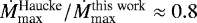 . Moreover, inspection of their table A.1, where they also list rates derived by a few other studies, seem to notreveal any major systematic discrepancies. Similarly, Crowther et al. (2006) also used Hα to derive Ṁmax (using unclumped CMFGEN models); here, for the 9 overlapping stars, all within Teff = 15 500–29 000 K, we find an average
 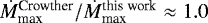 . As such, although the scatter is large it seems unlikely that the big discrepancies between observations and theory found for BSG mass-loss rates should be caused by any systematic effect specific for our study here (even though considerable uncertainties exist for various individual objects, see Table 6 and discussions in Appendix A).
As just one specific example, for HD 198478 with Teff = 17 500 K we derive an interval (see Table 7, and discussion in Appendix A) Ṁmax = 0.14–0.38 × 10⁻⁶ M⊙ yr−1. This agrees well with the interval Ṁmax = 0.12–0.41 × 10⁻⁶ M⊙ yr−1 obtained by Markova & Puls (2008) from their unclumped Hα analysis. Direct application of Geneva approach discussed above to HD 198478 places this star at the cool side of the second bi-stability jump (see dotted-lined source in Figs. 8 and 9); as such, even when using the empirical upper-limit υ∞ = 470 km s−1 from Table 6, the recipe predicts a very large  = 6.38 × 10⁻⁶ M⊙ yr−1, causing the large discrepancy visible in Fig. 8 (see top panel). Even if the star is placed in the ‘Fe III’ region, i.e. when MESA and Fixed-jumps approaches are used, the recipe would still return a rate,
  , that is more than an order of magnitude higher than the empirical upper limit (middle and bottom panel in Fig. 8). This shows that the reason we find large discrepancies between Ṁmax and
  for BSGs, but not for OSGs, is because of the large predicted
  increase when crossing the bi-stability jump regions.
In fact, when inspecting the so-called wind-performance number η = Ṁ υ∞/(L*∕c) for our sample (Fig. 9) we find a gradually decreasing trend –albeit again with significant scatter– with decreasing Teff, and do not see any evidence for sudden increases, or a secondary local maximum (e.g. Benaglia et al. 2007), at any of the predicted bi-stability limits. This is quite similar to the findings by Crowther et al. (2006); Markova & Puls (2008) and Haucke et al. (2018), who also did not find any empirical evidence for a sudden mass-loss increase with decreasing Teff. Note that, although the difference between theoretical predictions and empirical values is reduced when setting the central temperatures for the first and second bi-stability jumps at ~22 and ~10 kK respectively,the observed discrepancies for B supergiants are still considerable.
These large discrepancies may thus point toward a problem with current theoretical mass-loss rate predictions around the first bi-stability jump, regardless of its exact location, rather than toward issues related to empirical mass-loss determinations for BSGs derived by different authors and methods. This suggests that the basic mechanism responsible for increasing the mass-loss rate at the bi-stability jump (essentially recombination of iron) needs to be revisited in future work, preferably by locally consistent hydrodynamic calculations that do not assume a pre-described β velocity law. This is important also in view of the quite big role this bi-stability Ṁ increase plays in general stellar evolution modelling (see e.g. Vink et al. 2010; Keszthelyi et al. 2017).
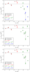 |
Fig. 8 Fromtop to bottom, empirical to theoretical mass-loss rates ratio, in logarithmic scale, as a function of effective temperature for the OB supergiants sub-sample. Empirical mass-loss rates correspond to the Ṁmax derived in this work. Theoretical mass-loss rates, |

5.2.1 Impact of clumping in scaling the derived upper-limit mass-loss rates
As mentioned above, the empirical values of the maximum OSG mass-loss rates derived from radio fluxes agree (within uncertainties) with the theoretical predictions by V00 and V01 (see also P06). However, ‘real’ agreement would only be true if the outermost wind of OSGs were unclumped. We note again that our Ṁmax estimates were obtained normalising the clumping stratification to the outermost wind region by setting  =
=  = 1. Therefore, if instead this region is affected by clumping, downward corrections become necessary. Hydrodynamical wind models extending all the way to the radio-emitting regions suggest typical factors of about
  ≈ 4–9 (Runacres & Owocki 2002, 2005). These models, however, were calculated assuming an unperturbed lower boundary at the stellar surface, and so it remains to be seen whether effects from, for example, a turbulent photosphere could persist all the way out to the radio region (see also discussion in Sect. 5.1.3). Assuming for now the outer-wind values from Runacres & Owocki (2002, 2005), the Ṁmax estimates of this paper would need to be scaled down by a factor ≈2–3. We re-emphasise that these typical
  ≈ 4–9 only refers to the outermost wind. Clumping factors predicted for the inner wind regions are typically significantly higher; for example, in the O-star simulations by Driessen et al. (2019) fcl peaks around r∕R*~ 1.5−2 and the average value for the innerwind (r∕R* = 1−2) is fcl ≈ 15−20. Thus, O-star mass-loss rates derived from unclumped models of inner-wind diagnostics (e.g. using optical recombination lines like Hα) should be scaled down more than corresponding radio rates. This is consistent with the empirical finding here that clumping factors on average are higher in the inner wind regions than in the outer ones. Typical reductions of ≈ 2−3 would agree well with the new theoretical mass-loss rate predictions for O-stars by Björklund et al. (2021) (see also Sander et al. 2017 and Sundqvist et al. 2019), as well as with various multi-wavelength empirical studies such as Najarro et al. (2011) (see Figs. 12 and 13 in Björklund et al. 2021). As demonstrated by Fig. 8, however, the situation is very different for BSGs, where
  can be overestimated by as much as 2 orders of magnitude. Of course, if the outermost wind of BSGs should be significantly clumped, this discrepancy would become even larger. For example, assuming the same clumping degree in the outermost wind as for OSGs (but see Driessen et al. 2019), current theoretical Ṁ predictions by V00 & V01 (the standard rates used in most evolutionary models), would be overestimated by factors 6–200 in case of the Geneva implementation.
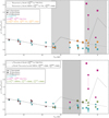 |
Fig. 9 Top: empirical-maximum (Ṁmax) and theoretical ( |

6 Summary and conclusions
We have constrained clumping properties of the intermediate stellar winds for a sample of 25 OB supergiants, giants, and dwarfs stars by using Herschel-PACS flux measurements at 70, 100, and 160 μm. For the analysis, we followed the approach developed and further tested it, by P06, assuming optically thin clumping. Additional available continuum observations in the literature from optical to radio wavelengths further allowed us to perform a consistent analysis and to derive robust estimates for the (minimum) wind-clumping structures at r ≳ 2 R*, as well as maximum mass-loss rate estimates ( =
=  = 1).
= 1).
Accurate radio emission measurements allowed us to derive precise Ṁmax values and to infer robust clumping structures for 17 of the 25 stars in our sample. In addition, millimetre flux observations for seven of these stars led to better constraints on the outer wind region (15 ≲r/R* ≲ 50), providing a precise determination of the radial stratification of the clumping at r ≳ 2 R*. Our major findings can be summarised as follows:
The stellar wind at r ≳ 2 R* for most of the stars in our sample fulfills the clumping stratification condition
 ≳
≳ ≿
≿ =
=  , regardless of the strength of the wind. The exceptions correspond to non-thermal or variable thermal sources, such as HD 37043 (binary), HD 193237 (LBV), and CygOB2#12 (eBHG).
The clumping-degree drop from the intermediate (
 ) to the outer wind region (
 ) depends on the spectral type and luminosity class: on average,
  is ≈ 4 times larger than
  for OSGs, ≈ 2 times larger for BSGs, and similar to
  for OB dwarfs and giants.
Our findings agree well with the empirical clumping properties at r ≳ 2 R* derived by Najarro et al. (2011) and Clark et al. (2012) following a different parametrisation. In addition, our results overall support the hydrodynamical OSG models by Sundqvist & Owocki (2013), where clumping starts to decrease at r ≈ 2–6 R*, and, tentatively, the recent 1D LDI simulations of OSG and BSG winds by Driessen et al. (2019), which predict lower amounts of clumping in BSGs.
We found that for eight OB supergiants in our sample
 >
> . This significantly extends the findings of P06 in just one star of their sample (ζ Pup) and is inagreement with the empirical clumping properties by Najarro et al. (2011) and the theoretical predictions for OSGs by Sundqvist et al. (2011) and Sundqvist & Owocki (2013). This suggests that such a behaviour, rather than being an exception, could imply the existence of two trends characterised by different physical conditions at the base of the wind.
For OSGs the derived upper-limit mass-loss rates, Ṁmax, agree with the theoretical predictions by V00 and V01 for unclumped winds, whereas BSGs show a discrepancy which severely increases with decreasing effective temperature: the estimated Ṁmax starts to differ from theoretical recipes in the predicted first bi-stability transition zone, and up to 1.5–2 orders of magnitude lower for the coolest B supergiants below the first bi-stability jump. Since the empirical scaling invariant is
 and our derived mass-loss rates are upper limits assuming an unclumped radio-emitting wind (
 ), any clumping in this outermost region would only increase this discrepancy.
A key conclusion of our analysis regards the upper-limit mass-loss rates of OSGs and BSGs derived from radio emission. Although the actual empirical Ṁ will depend on the level of clumping in the outermost wind, these upper limits should be quite robust since radio emission is a relatively ‘clean’ diagnostic. This thus allows us to perform important empirical testing of theoretical mass-loss predictions across the so-called bi-stability jumps (see previous sections).
If the absolute value of clumping in the outermost wind region of OB supergiants was  = 4–9, as suggested by the hydrodynamic O-star models by Runacres & Owocki (2002, 2005), the theoretical mass-loss rate recipes by V00 and V01 would be overestimated by a factor 2–3 for OSGs; as discussed above, this would then agree well with the recent theoretical O-star mass-loss predictions by Björklund et al. (2021). On the other hand, the consequences for BSGs across the bi-stability regions are dramatically independent of their clumping properties, and temperatures of the jumps, since these objects require downward
  corrections of up to 1.5–2 orders of magnitude, even in the case in which BSGs were not as clumped as OSGs (Driessen et al. 2019). Thus, this finding calls for an urgent re-investigation of the role recombination of iron-like elements plays in determining the mass-loss rates of objects that cross the bi-stability region, as well as a careful analysis of corresponding effects for stellar evolution models (Keszthelyi et al. 2017).
Regarding future diagnostic studies, the next step is to further investigate the clumping degree also in the inner wind, and to compute actual, absolute values of fcl(r). To achieve this, our team is collecting archival and missing observations throughout the spectral range, including X-ray emission. Multi-wavelength analysis, optical to radio continuum fitting as applied in this work, and UV to NIR spectroscopy in combination with state-of-the-art model atmosphere codes including an adequate treatment of wind clumping will then allow for precise determinations of clumping factors and the actual mass-loss rates of OB stars.
Acknowledgements
M.M.R-D gratefully acknowledges J. A. Fernández-Ontiveros for his invaluable insights and help at earlier stages of the paper. This research was partially supported by from a FPI-INTA fellowship, and the Spanish MICINN through grants AYA2008-06166-C03-02, AYA2010-21697-c05-01 and FIS2012-39162-C06-01. F.N. and M.M.R.-D. acknowledge financial support through Spanish grants ESP2017-86582-C4-1-R and PID2019-105552RB-C41 (MINECO/MCIU/AEI/FEDER) and from the Spanish State Research Agency (AEI) through the Unidad de Excelencia “María de Maeztu”-Centro de Astrobiología (CSIC-INTA) project No. MDM-2017-0737. J.O.S. acknowledges support from the Odysseus program of the Belgian Research Foundation Flanders (FWO) under grant G0H9218N, support from the KU Leuven C1 grant MAESTRO C16/17/007, and previous support from the European Union Horizon 2020 research and innovation program under the Marie-Sklodowska-Curie grant agreement No 656725.
Appendix A Fitting individual objects
In the following, we provide detailed comments on our fits to the individual objects. For those sources previously analysed by P06 through the same procedure, we also provide the best so- lutions derived by these authors. The fit-diagrams of OSGs are displayed in Figure A.4, BSGs in Figures A.5 and A.6, O Giants in Figure A.7, OB Dwarfs in Figure A.8, and the two confirmed binaries in Figure A.9. The results of the fixed-regions approach are summarised in Table 6, and those of the adapted-regions ap- proach in Table 7. Distances, colour excesses and extinction parameters are listed in Table 3.
A.1 O supergiants
HD 66811 (ζ Pup)
This source was previously analysed by P06. Therefore, we follow a procedure like that also described in Section 3.2 of the main text: first we test the clumping stratification derived by these authors (see their Table 7) against new PACS flux observations at 70, 100 and 160 μm (magenta diamonds indiagrams) together with additional observations at MIR (AKARI & WISE catalogues) and at 2 and 6 cm (Morton & Wright 1978, 1979, Bieging et al. 1989) available in the literature (green circles in diagrams). Since all radio measurements are well determined, Ṁmax is also definite.
In Figure A.4, we plot the two derived solutions in the fixed- (solid line) and adapted-regions (magenta-dotted line) ap- proaches, and P06’s best-fit solution (blue-dashed line) for the shorter distance: Ṁmax = 4.2 × 10⁻⁶ M⊙ yr−1,  = 5,
= 5,  = 1.5,
  = 1.4 and
  = 1 with rin = 1.12 R*, rmid = 2 R*, rout = 15 R* and rfar > 50 R*. We note that the clumping factor at the intermediate region
  derived by P06 leads to an underestimation of the FIR fluxes.
Our best solution is obtained in the adapted-regions approach for the same values of Ṁmax and  as derived by P06, and a larger intermediate clumping factor. Provided the clumped wind is restricted to 1.12 ≲ r/R* ≲ 12, then derived values are those given in the first entry in Table 7. For the fixed-regions approach, the best possible solution is also achieved for the same values of Ṁmax and clumping factors, but with a slightly worse χ2, see the first entry in Table 6. Identical results are ob- tained for the alternative solution provided by P06 (see first entry in their tables 1 and 7) corresponding to the larger distance of ζ Pup, d = 0.73 kpc: Ṁmax = 8.5 × 10⁻⁶ M⊙ yr−1,
  = 5,
= 5,  =
=  = 1 and
  = 3.1 and 3.2 for the adapted- and fixed-regions approaches. Despite the scaled values of Ṁmax and R* for this alternative distance, the radial clumping structure and optical depth invariant, Q′, are conserved.
As pointed out above, the IRAS measurements used by P06 were not colour-corrected, whereas we performed the colour correction for IRAS observations at 12, 22 and 60 μm, leading to slightly lower flux values than those used by P06. However, this difference does not lead to significant changes in the derived clumping structure. Note that, although this source is well constrained, only additional mm and radio observations can help disentangling whether the ‘odd’ measurements at 160 μm and 2 cm are corrected (or not), or if they perhaps respond to variable thermal emission from the source.
CygOB2#11
This source was previously analysed by P06. Since the measured fluxes at 3.5 and 6 cm are well determined, Ṁmax is definite. However, only upper limits for the fluxes at 70, 100 and 160 μm can be estimated from the PACS observations, thus the clumping properties in the intermediate wind region remain unconstrained. Despite this, we tested the best solutions derived by P06 against additional measured fluxes at MIR wavelengths from the literature (Spitzer, WISE, and MSCX6 catalogues). There is a recent estimated distance for this source by GAIA, d = 1.72 kpc, which is roughly the same value as used by P06, d = 1.71 kpc; as such, only a very small scaling-factor for Ṁmax and R* is needed to account for the updated distance.
The corresponding panel in Figure A.4 displays the best- fit solution by P06 (magenta-dotted line) and our derived best-fit solution (solid line), corresponding to the fixed-regions ap- proach. Themaximum mass-loss rate estimated by P06 is consistent with all radio fluxes and the upper flux limits at FIR wavelengths (flux emission model well below the upper limits). However, the clumping structure derived by the authors starts to depart from observations beyond 10 μm, overestimating the measured fluxes up to 25 μm and marginally matching the measured flux at 30 μm. Our best-fit solution is achieved in the fixed- regions approach for a constant and minimum clumping degree throughout the entire wind, i.e.  =
=  =
=  =
=  = 1. The maximum mass-loss rate is only marginally different from P06’s estimate.
Although our FIR flux estimates are only upper limits, the maximum clumping degree consistent with observations at the intermediate wind region is  = 3, a factor ≈ 1.7 lower than the value derived by P06. Note that only additional observations at FIR up to ~ 1.3 mm can help properly constrain the clumping properties at the intermediate wind region, although our simulations point to a lower clumping degree than previous estimates in that region. Finally, the large measured flux at 10.9 μm (Leitherer & Wolf 1982) is still not reproduced by any model, and thus either is affected by some problem (i.e. artefacts, contamination, etc.), or it could be related to warm dust emission. The former is more likely since the nearby flux estimates at 9 and 11.02 μm are consistent with a lower flux emission model for the source, and with the rest of flux observations at MIR.
HD 210839 (λ Cep)
This source was also analysed by P06, and a new distance estimate from GAIA is available. Figure A.1 displays the best-fit solutions from this work and by P06 for the distance used by these authors. In Figure A.4 we present our best-fit models for the GAIA distance used in this work.
From the well determined radio measurements, P06 estimated a well defined maximum mass-loss rate for this source. Due to the two different SCUBA fluxmeasurements at 1.3 mm, the authors provided two alternative solutions for the clumping structure in wind region 4. Thus, for Ṁmax = 3 × 10⁻⁶ M⊙ yr−1 (d = 1.08 kpc) their best-fitsolution assumes  = 6.5,
  = 10 and
  = 1 with rin = 1.05 R*, rmid = 4 R*, rout = 15 R* and rfar > 50 R*. With
  = 1 (blue-dashed line in Figure A.1), the lower SCUBA value, the 0.7 cm and the radio flux values are reproduced, whereas with
  = 8, the upperSCUBA and all radio fluxes are well fitted, but the 0.7 cm flux is overestimated (orange dashed-dotted line in Figure A.1). Using our new flux values, Figure A.1 shows that the P06 mass-loss rate is consis- tent with the added flux at 21 cm, whereas their clumping stratification marginally matches the flux measurements at MIR andFIR wavelengths, but perfectly fits radio observations. In addition, the new measurement at 160 μm is consistent with the upper SCUBA value, which does not help to properly constrain the clumping degree for Region 4. However, both 160 μm and SCUBA fluxes have large errors13, preventing us from drawing any further conclusions.
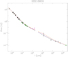 |
Fig. A.1 Comparison between the best-fit solutions for HD 210839 by P06 (blue-dashed and orange-dotted-dashed lines) and our best-fit solutions (solid and magenta-dotted lines) for the same value of the distance (see text). Magenta diamonds are our measured FIR fluxes at 70, 100 and 160 μm. Black squares and green circles indicate flux values from the literature. For those sources in common with P06, green circles indicate new available data added to the analysis. Arrows indicate upper limits. |
In the following, the described clumping structure refers to the fixed-regions approach. The best-fit solution is achieved for the minimum possible clumping degree for the inner and outermost wind regions, and a larger clumping for the intermediate one,  =
=  =
=  = 1 and
  = 7 (solid line inFigures A.1 and A.4). In Region 4, although a minimum clumping factor provides the best-fit solution, the clumping degree could range from 1 to 8, with a maximum value also ranging from 5 to 12. Thus, with
  = 1 or
  = 8, the lower (solid line in Figures A.1 and A.4) or the upper (magenta-dotted line in Figures A.1 and A.4) SCUBA value are respectively matched.
  = 5 – 12 is still consistent with the 160 μm and with both SCUBA fluxes, respectively. Only extra flux observations at sub-mm and mm spectral ranges can help derive definite estimates for wind region 4. For the new distance estimate from GAIA, d = 0.62 kpc, the corresponding scaled maximum mass-loss rate is Ṁmax = 1.3 × 10⁻⁶ M⊙ yr−1, and the same clumping properties described above (Table 6) provide the best-fit solutions (Figure A.4).
HD 152408
The flux observations at 2 and 6 cm are well determined, thus Ṁmax is definite. In the corresponding panel in Figure A.4, we present our best-solution fitting all the data (magenta-dotted line) and the best possible one in the fixed-regions approach (solid line), respectively. The maximum mass-loss rate is 9.5 × 10⁻⁶ M⊙ yr−1 one of the largest values in the sample. For the fixed-regions approach the best solution is obtained by setting  =
=  =
=  = 1, and
  = 3.25 (Table 6). However, the best-fit solution for HD 152408 is achieved for the adopted-regions approach by slightly increasing to
  = 3.8, provided that the inner wind region is extended to rmid = 3.5 R* (Table 7). The SCUBA measurement (1.3 mm) further allows us to constrain the maximum possible value of the clumping degree in Region 4 to
  = 3.
= 3.
HD 151804 (V973 Sco)
Discussed in detail in the main text.
HD 30614 (α Cam)
This source was analysed by P06, and we therefore show P06’s best solution together with our best-fits models. It can be observed in the fit-diagram that P06’s solution underestimates fluxes at MIR and FIR wavelengths, and that although their Ṁmax is still consistent with the additional measured fluxes at 6 cm 14, the additional radio flux at 21 cmpoints to a slightly larger Ṁmax. We found that a value of Ṁmax= 1.75 × 10⁻⁶ M⊙ yr−1 with  = 6,
= 6,  = 3.3 and
  =
= = 1, provide the best possi- ble solution in the fixed-regions approach (solid line; Table 6). However, the best-fit solution (magenta-dotted line) for the estimated Ṁmax is achieved by extending tormid= 4 R*, so that
  = 6 and
  =
=  =
=  = 1 (Table 7). In all simulations the maximum value of
  is constrained by
  =2.
=2.
A.2 B supergiants
HD 37128 (ϵ Ori)
There are well determined available radio fluxes for this source, therefore Ṁmax is definite. For Ṁmax = 1.25 × 10⁻⁶ M⊙ yr−1, we present the two fit-solutions consistent with all the data, corresponding to the fixed- (solid line) and the adapted-regions (magenta-dotted line) approach, respectively (Figure A.5). For the fixed-regions approach, the best possible solution corresponds to a 1 (Table 6). The best-fit solution, however, is obtained in the adapted-regions approach by increasing a factor 2 the clumping degree in the intermediate wind region,  = 5,
= 5,  = 8 and
  =
=  = 1, provided that rout = 8 R* (Table 7).
HD 38771 (κ Ori)
Only one radio observation, an upper limit at 6 cm, is available for this source. Thus, only an upper limit for Ṁmax is provided. The panel corresponding to this star in Figure A.5 shows the fit-solutions for both the fixed- (solid line) and the adapted-regions (magenta-dotted line) approach. We estimated Ṁmax ≲ 0.7 × 10⁻⁶ M⊙ yr−1. For this upper limit, the best possible solution in the fixed-regions approach corresponds to a significantly clumped inner wind,  = 8, and
  =
=  =
=  = 1 (Table 6). The best-fit solution is achieved in the adapted-regions approach, with a considerable large clumping degree in the inner wind region,
  = 20, and again
  =
=  =
=  = 1, provided that rmid = 1.55 R* (Table 7). Despite of the lack of flux observations from 100 μm to radio wavelengths,
  = 8 is still consistent with all data. Only mm and well-determined radio flux measurements can provide definite Ṁmax and the clumping structure of the outer wind for this source.
HD 154090 (κ Sco)
Only one radio measurement is available at 3.5 cm, but it is well determined and thus Ṁmax is definite. Figure A.5 displays fit-solutions for both the fixed- (solid line) and the adapted-regions approach (magenta-dotted line). For Ṁmax = 1. × 10−6 M⊙ yr−1, a moderate clumping degree in the inner and the intermediate wind regions,  = 2 and
  = 4.5, and
  =
=  = 1, provide thebest possible fit solution in the fixed-regions approach (Table 6). The best-fit solution for this source is achieved in the adapted-regions approach, with a moderate, and almost constant, clumped wind restricted to r ≲ 15 R*,
  = 4,
= 4,  = 3.5 and
  =
=  = 1, provided that rin = 1.4 R* instead of rin = 1.05 R* (Table 7). In the absence of sub- and mm observations,
  = 8 is still consistent with the 70 and 100 μm and 3.5 cm fluxes. Only additional flux observations at mm can better constrain wind region 4.
HD 193237 (P Cyg)
Discussed in detail in the main text.
HD 24398 (ζ Per)
Discussed in detail in the main text.
HD 169454
This source is one of the four eBHGs in our sample. The available radio fluxes at 2 and 6 cm are well determined, and thus Ṁmax is definite. In Figure A.5 we present fit-solutions for the fixed- (solid line) and the adapted-regions (magenta-dotted line) approach. For Ṁmax = 10.4 × 10⁻⁶ M⊙ yr−1, the best pos- sible solution in the fixed-regions approach is provided for a weak intermediate clumped wind,  = 2.5, and an unclumped inner and outer wind,
  =
=  =
=  = 1 (Table 6). However, a slightly better solution is obtained in the adapted-regions approach, by increasing the clumping degree only in the intermediate wind region,
  = 4.5, provided it begins at rmid = 4 R* (Table 7). In all simulations, the single mm flux estimate (at 1.3 mm) constrains the maximum clumping degree in Region 4, still consistent with all data,
  = 2.5
= 2.5
HD 152236 (ζ1 Sco)
This star is another of the four eBHGs in our sample. For the well determined radio measurements, we obtain Ṁmax = 6.2 × 10⁻⁶ M⊙ yr−1. Figure A.6 displays the derived solutions for the fixed- (solid line) and the adapted-regions approach (magenta-dotted line). For the fixed-regions approach, we obtain a weak clumping degree in the intermediate wind region,  = 2.8, and
  =
=  =
=  = 1 (Table 6). However, a slightly better solution is obtained in the adapted-regions approach with a marginally larger clumping factor in the intermediate wind region, provided that it is restricted by rout = 10 R* (Table 7).
HD 41117 (χ2 Ori)
All available radio measurements are well determined, and therefore Ṁmax is definite. For Ṁmax = 1.8 × 10⁻⁶ M⊙ yr−1, the best-fit solution is achieved in the fixed-regions approach for  = 7.3,
  = 1.35 and
  =
=  = 1 (solid line inthe corresponding panel in the Figure A.6). The lack of observations in the sub- and mm regime lead to
  = 6 consistent with FIR and radio observations at 2 cm.
HD 194279
Our measured fluxes at 70 and 100 μm are lower than theoretical predictions for an homogeneous, unclumped wind, whereas the available, well-determined radio fluxes at 3.5 and 6 cm are consistent with those. We derived two solutions intending to fit consistently the FIR and/or radio fluxes (corresponding fit-diagram in Figure A.6). The described clumping structures below correspond to the fixed-regions approach, which provides the best-fit solution for this source.
A first solution (solid line), matching radio observations, is provided for Ṁmax = 2.12 × 10⁻⁶ M⊙ yr−1 and for a constant  =
=  = 1 (first entry Table 6). However, it can be observed that although this solution reproduces the radio fluxes, it only hardly matches the flux measurement at 70 μm, and overestimates the one at 100 μm.
A second, and better solution (magenta-dotted line), is achieved for a much lower Ṁmax = 0.505 × 10⁻⁶ M⊙ yr−1. For this value, the minimum clumping degree at r ≲ 15 R* and a strong one at r ≳ 15 R*, perfectly match all observations, i.e.  =
=  = 1 and
  =
=  = 20 (second entry in Table 6).
The second solution fits all flux observations throughout the wind and provides the best-fit for this source. However, if this is the case, HD 194279 is the only single star and radio thermal emitter in our sample with such a high clumping degree in the outer wind regions (r ≳15 R*). On the other hand, if HD 194279 turned out to be a non-thermal emitter, then this clumping structure would follow the same trend found for the other non-thermal emitters in our sample as HD 37043 (SB) or CygOB2#12. Due to the scarcity of flux observations of HD 194279 at large wavelengths, the high uncertainties derived in the estimated FIR fluxes and the fact that the two radio measurements are consistent with thermal emission, we consider the constant clumping degree solution to be more likely (first entry in Table 6). Only re-observing at FIR and radio wavelengths can help discriminating between these scenarios.
HD 198478
Due to its stellar pulsation activity this star has variable spectral profiles, so that the stellar and wind parameters obtained via optical spectroscopic analysis show substantial scatter (Crowther et al. 2006, Markova & Puls 2008, Kraus et al. 2015). This is not due to the different approaches to derive stellar parameters, but to the phase of activity of the source when spectra where taken.
In order to study how different input values affect the estimated Ṁmax and clumping structure, we use the range of input parameters as provided by Markova & Puls (2008). In Table A.1 we present our fit solutions in the fixed-regions approach for each combination of υ∞, β and YHe by these authors. The two diagrams in Figure A.2 display the corresponding solutions present in Table 6. For clarity, in Table 6 we indicate the full range for derived Ṁmax and clumping factors, and Figure A.6 presents fit-solutions corresponding to the lowest (magenta-dotted line) and the largest (solid line) Ṁmax.
Only two radio flux measurements at 3.5 and 6 cm are available (Scuderi et al. 1998), and both are upper limits. There- fore, the resulting Ṁmax is an upper limit. The minimum χ2 ob- tained for the different solutions in Table A.1 are only marginally different (solid and magenta-dashed lines in Figures A.2 and A.6). Note that although the absolute values of clumping fac- tors change, the overall clumping properties throughout the en- tire wind are conserved, and the largest difference in  and
and  is a factor of 1.33.
Regarding Ṁmax, the largest difference, a factor 2.7, arises from simultaneously changing υ∞ and YHe (first and last entry in Table A.1). However, for a given velocity field (υ∞ and β) and a factor of 2 different helium-fraction, Ṁmax and clumping factors vary only by ~ 15% and less than 12%, respectively. Moreover, in all simulations the clumping degree in the outermost wind remained constant, i.e.  =
=  = 1 for r ≳ 15 R*, with
  = 10 (blue-dashed line in Figure A.6). Therefore, we are confident that the presented Ṁmax ranges and clumping properties are reliable.
Minimum clumping structure and Ṁmax of HD 198474 derived in this work for the interval of stellar parameters provided by Markova & Puls (2008) (see text and Figure A.2).
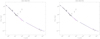 |
Fig. A.2 Observed and best-fit fluxes vs. wavelength for HD 198478 depending on the input parameters used in the simulations (see Table A.1 and text in Appendix A.2). Colours and symbols as in Figure A.1. Left: Best-fit models 470 kms−1 for YHe = 0.2 (solid line; Sol. 1a) and YHe = 0.1 (magenta-dotted line; Sol. 1b). Right: Best-fit models for υ∞ = 200 kms−1 for YHe = 0.2 (solid line; Sol. 2a) and YHe = 0.1 (magenta-dotted line; Sol. 2b). The blue-dashed line in both plots shows how changes in YHe are reflected in the emission flux model. |
In summary, qualitatively the observed SED for HD 198478 can be perfectly reproduced with a strong clumping degree in the innermost wind region, moderate clumping in the intermediate one, and the minimum clumping degree in the outermost ones, with a range of mass-loss rates (maybe a reflex of mass-loss episodes due to stellar pulsations).
HD 80077
The available radio measurements at 3.5 and 6 cm for this eBHG are well determined, and thus Ṁmax is definite. The best-fit model is obtained in the fixed-regions approach (solid line in corresponding panel in Figure A.6). For Ṁmax = 3.45 × 10⁻⁶ M⊙ yr−1 a weak clumped inner and intermediate wind,  = 2.5 and
  = 1.8, and an unclumped outer one,
 =
=  = 1 (Table 6) perfectly match the SED of this source. Due to the lack of observations at sub- and mm-wavelengths we estimated that
  = 6 is still consistent with the observed 70 and 100 μm, and 3.5 cm fluxes (magenta-dotted line). Only flux observations at mm regime will better constrain this wind region.
HD 53138 (o2 CMa)
There are no mm or radio observations available for this source. Therefore, our analysis only provides an upper limit for the maximum mass-loss rate consistent with the observed fluxes at the largest possible wavelengths (at 70 and 100 μm). In the corresponding panel in Figure A.6, we present the solutions for both the fixed- and adapted-regions approaches (solid and magenta-dotted line, respectively).
For Ṁmax = 1.8 × 10⁻⁶ M⊙ yr−1, the fixed-regions approach yields  = 2, and
  =
=  =
=  = 1 (Table 6). The best-fit solution, however, is achieved in the adapted-regions ap- proach by slightly increasing the clumping degree in the inner wind region,
  = 3 and
  =
=  =
=  = 1, provided that rmid = 1.3 R* (Table 7). Due to the lack of observations of this source at λ > 100 μm,
  = 18 at r ≳ 15 R*, and
  = 50. Only mm and radio observations will definitively constrain the Ṁmax and the clumping structure of the outer wind of this source.
CygOB2#12
This is an exotic eBHG15 which, in addition, is suspected to be a non-thermal or variable thermal source; several authors have reported short term variations in the measured radio fluxes (Bieging et al. 1989, Scuderi et al. 1998), and more recently Morford et al. (2016) detected flux variations of ~ 14 days at 21 cm. However, the nature of this variability, whether it is due to changes in the state of ionisation of the wind like in P Cyg, or by the object being a non-thermal source (maybe a binary), still remains to be unveiled.
In the corresponding panel in Figure A.6, we present the best possible solutions in the fixed-regions (solid and magenta-dotted lines) and the adapted-regions approaches (blue-dashed and orange-dashed-dotted lines). CygOB2#12 is one of the sources in our sample for which Ṁmax is constrained by in- frared fluxes instead of by radio ones. We noted that the mass-loss rate required to match the estimated low flux at 21 cm, Ṁmax ~ 2.4 × 10⁻⁶ M⊙ yr−1, overestimates by large the ob- served fluxes at MIR. From MIR and FIR fluxes, we derived Ṁmax = 1.02 × 10⁻⁶ M⊙ yr−1.
For this Ṁmax, the fixed-regions approach yields  = 1,
= 1,  =
=  = 10 and
  ranges from 5 to 15 (Table 6) to consistently reproduce the variable radio flux values (solid and magenta-dotted lines, respectively). The best-fit solution, however, is achieved in the adapted-regions approach for a larger clumping degree in the intermediate wind region,
  = 1,
= 1,  = 12,
= 12,  = 10 and
  = 5 – 15 (blue-dashed and orange-dashed-dotted lines, respectively), provided that rmid = 2.5 R* and rout = 8 R* (Table 7). In all simulations the flux at 1.3 mm constrains
  = 12.
= 12.
A.3 O Giants
HD 24912 (ξ Per)
The clumping stratification of this source was also analysed by P06. These authors derived two possible solutions from fitting the variable upper limits of the radio flux estimates at 0.7, 2, 3.5 and 6 cm. In Figure A.3 we show these best-fit solutions from PO6. The first solution (solid line) is consistent with the larger radio upper flux limits, and the second one (magenta-dashed line) with all radio upper flux limits. It can be observed that both solutions by P06 overestimate our new flux estimates at 70 and 100 μm and, moreover, that the additional and well de- termined fluxes at 3.6 cm and 21 cm used in our analysis seem to confirm variable radio emission from this source. Note that although these new radio observations are slightly larger (which can be due to either calibration effects or real radio variability of the source), they are also consistent with the upper flux limits previously detected at the radio regime. Moreover, since the ra- dio fluxes estimated for other sources in our sample (λ Cep and α Cam) by Schnerr et al. (2007) are consistent with the existing radio observations by different authors at different wavelengths, we are also confident in the estimated values provided by the authors for this source.
We obtain Ṁmax = 1.4 × 10⁻⁶ M⊙ yr−1. In order to fit the aforementioned variable radio fluxes we derived several so- lutions for the clumping structure. The corresponding fit- diagram in Figure A.7 displays our fit-solutions in the fixed-regions (solid and magenta-dotted lines) and adapted-regions approaches (blue-dashed and orange dashed-dotted lines). In the fixed-regions approach an almost constant and moderate clumping degree for the entire wind,  =
=  = 3.5 and
  =
=  = 3 (second value in Table 6), fits perfectly the upper flux limits and the well determined measurement at 21 cm (magenta-dotted line in Figure A.7), whereas a moderate clumped wind restricted to r ≲ 15 R* and an unclumped outer one,
  =
=  = 3.5 and
  =
=  = 1 (first value in Table 6), are consistent with all radio fluxes but the flux value at 21 cm (solid line in Figure A.7).
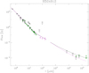 |
Fig. A.3 Comparison between the best-fit solutions for HD 24912 (ξ Per) by P06(solid and magenta lines, see text) and our flux estimates at 70, 100 and 160 μm (magenta diamonds). Colours and symbols as in Figure A.1. |
The best-fit solution for this source, however, is achieved in the adapted-regions approach for a much more structured clumped wind. For the estimated Ṁmax, a significantly clumped inner wind,  = 5, and a constant
  =
=  =
=  = 1 (first value in Table 7) provide the best-fit solution consistent with all radio data but the flux value at 21 cm (blue-dashed line in Figure A.7), with rin = 1.1 R* and rmid = 4 R*. To fit the larger up- per radio flux limits and the flux at 21 cm (orange dashed-dotted lines in Figure A.7), the clumping degree for the outer wind re- gions have to be increased to
  =
=  = 3 (second value in Ta- ble 7). The lack of observations in the mm regime gives
  = 5.
= 5.
Finally, the new measured FIR fluxes for this source enforce a certain clumping degree within 1.05 – 1.1 ≲ r/R* ≲ 2 – 4. The observed variability at the MIR (from 4.6 to 11.4 μm) and radio regimes may be explained by means of either clumping or some other physical process such as co-rotational interaction zones or a wind compressed equatorial region, as suggested by P06. In particular, a potential magnetic field interacting with the stellar wind leads to wind confinement and channelling (ud-Doula & Owocki 2002, Owocki et al. 2008), and in presence of relativistic electrons, non-thermal synchrotron emission arises and may dominate the radio spectrum under certain conditions (Trigilio et al. 2004). Another possibility is that ξ Per is a binary system, or both magnetic field and colliding winds are present as some numerical simulations suggest (van Loo et al. 2005). However, positive magnetic field detections for ξ Per have not been reported so far, and there is no observational evidence of a close companion, although several sources in its surroundings have been detected. Therefore, the nature of this variability remains unanswered, and only mm and additional radio observations can help ascertain it.
HD 36816 (λ Ori A)
This source was previously analysed by P06, and there is a new distance estimate available from GAIA. All radio flux obser- vations are upper limits, and consequently the estimated Ṁmax is an upper limit. In the right panel in Figure A.7 we present P06’s best-fit solution (magenta-dotted line) and the best-fit model de- rived in thiswork (solid line), corresponding to the fixed-regions approach.
P06 derived Ṁmax ≲ 0.4 × 10⁻⁶ M⊙ yr−1 (for d = 0.5 kpc) and  = 2,
= 2,  =
=  =
=  = 1 (with rin = 1.05 R*, rmid = 2 R*,rout = 10 R* and rfar > 50 R*). Moreover
  = 20 and
  = 2 (blue-dashed line), respectively. The clumping strati- fication derived by P06 for the upper limit Ṁmax is consistent with the additional MIR observations available, but slightly overestimates the obtained fluxes at 70 and 100 μm. The best-fit solution, however, is found by decreasing the clumping degree in the inner wind region to
  =
=  =
=  =
=  = 1.
= 1.
There are no well-defined flux observations available at wavelengths larger than 100 μm. Despite that, we can lower the maximum clumping degree for the intermediate and outer wind regions derived by P06 to  = 5 and
  = 2. Only additional, and well determined observations at mm and radio regimes can provide definite Ṁmax and clumping factors in Regions 4 and 5,
  and
and  , respectively. For the GAIA distance used here, d= 0.27 kpc, the scaled upper limit maximum mass-loss rate becomes Ṁmax ≲ 0.16 × 10⁻⁶ M⊙ yr−1, and the derived clumping structure described above (Table 6) provide the best-fit solution.
A.4 OB Dwarfs
HD 149757 (ζ Oph)
All available mm and radio observations for this rapidly rotating source are upper limits, therefore Ṁmax is also an upper limit. We noted that if we derive Ṁmax to fit the radio upper limits at 6 cm, the flux-model emission is consistent with the observations from V- to NIR-band but overestimates fluxes at MIR and FIR wavelengths. Therefore, the upper limit Ṁmax is constrained by the fluxes at 70 and 100 μm. The left panel in Figure A.8 displays our best-fit solution, which corresponds to the fixed-regions approach. This best-fit solution (solid line) is obtained by Ṁmax ≲ 0.07 × 10⁻⁶ M⊙ yr−1 and a constant  =
=  =
=  =
=  = 1 (Table 6). This model reproduces all well-defined flux observations and is consistent with all upper limits in the radio regime.We also obtain
  = 20 and
  = 6 (magenta-dotted line). Additional well defined mm and radio fluxes are needed to derive definite Ṁmax and clumping properties in the outermost wind region.
HD 149438 (τ Sco)
τ Sco is a confirmed magnetic B-star (Petit et al. 2013), and a very slow rotator (~ 5 km s−1; Donati et al. 2006). Mass-loss rates found in the literature range from Ṁ = 0.0013 × 10⁻⁶ M⊙ yr−1 (from UV resonance lines; Hamann 1981), to Ṁ = 0.0614 × 10⁻⁶ M⊙ yr−1 (from optical spectroscopy; Mokiem et al. 2005), with a value in-between Ṁ = 0.02 × 10⁻⁶ M⊙ yr−1 (from NIR spectroscopy; Repolust et al. 2005). We note that all these derivations used non-magnetic wind models to derive the mass-loss rate, and thus did not take into account the considerable effect the magnetic field has upon the wind structure.
The right panel in Figure A.8 displays our best-fit models for this source, corresponding to the fixed-regions approach. Whereas the upper limits at 1 and 3 cm (Kurapati et al. 2017) are consistent with thermal emission, those at 6 cm (Bieging et al. 1989) and 13 cm (Kurapati et al. 2017) point to non-thermal emission. In view of the SED trend up to 160 μm, we suspect that the likely flux value at 13 cm is much lower than the upper limit provided by Kurapati et al. (2017), and therefore we do not attempt to fit it. Despite that, the upper flux limits from 1 to 6 cm still suggest τ Sco is a non-thermalemitter. Since it is a magnetic star, the observed radio variability might be explained by non-thermal synchrotron emission. However, non-thermal radio emission seems to favour centrifugal magnetospheres instead of dynamical ones (Kurapati et al. 2017), and τ Sco is classified as having a dynamical magnetosphere (Petit et al. 2013). Therefore, the detected variability and its nature still needs to be confirmed by deeper radio observations.
Nevertheless, we derived two possible upper limits for Ṁmax, attending to variable radio upper flux limits, and being consistent with the well determined fluxes at 70 and 100 μm. A first solution (magenta-dotted line) is obtained for a Ṁmax ≲ 0.315 × 10⁻⁶ M⊙ yr−1 and a constant  =
=  =
=  =
=  = 1 (first entry in Table 6). Although this model perfectly matches the observations at λ ≲ 100 μm and the upper limit at 6 cm, it overestimates by large the radio upper flux limits at shorter wavelengths. A second solution (solid line) is achieved for a much lower Ṁmax ≲ 0.018 × 10⁻⁶ M⊙ yr−1, an extremely large clumping degree in the inner wind region,
  = 300, and
  =
=  =
=  = 1 (second entry in Table 6). In this case, the model consistently reproduces all observations and the radio upper limits, but the flux at 70 μm only marginally, and slightly underestimates the one at 100 μm. The FIR fluxes and the radio upper limit at 6 cm could be perfectly matched with this value of Ṁmax by increasing the clumping degree of the wind at r ≳ 2 R* as
  =
=  =
=  = 300. However, the radio upper limits at 1 and 3 cm still remains overestimated by large. We caution, however, that none of the above takes into account any effects of the magnetic field upon the wind structure. Additional and well determine flux observations at mm and radio regime, along with proper magnetic modelling, may help reaching conclusive results regarding this source.
A.5 Binary OB stars
HD 149404
This source is a known massive spectral binary (Rauw et al. 2001, Raucq et al. 2016). From the only reliable radio observation at 3.6 cm we obtain Ṁmax = 8.27 × 10⁻⁶ M⊙ yr−1. The corresponding panel in Figure A.9 displays the best possible solution in the fixed-regions (solid line) adapted-regions approaches (magenta-dotted line). The best possible solution in the fixed-regions approach is obtained for  =
=  =
=  = 1 and
  = 5.4 (Table 6). The best-fit solution, however, is achieved in the adapted-regions approach (magenta-dotted line) by increasing the clumping degree in the intermediate wind region,
  =
=  =
=  = 1 and
  = 7, provided that it starts at rmid = 2.5 R* (Table 7). For both approaches,
  = 6 is still consistent with the data (blue-dashed line).
HD 37043 (ι Ori)
ι Ori is a known binary (Pittard et al. 2000, Pablo et al. 2017), with consistent observed variable flux at radio wavelengths. This source was previously analysed by P06 as a thermal emitter.
In the corresponding panel in Figure A.9, we present the two solutions derived by P06, together with our best-fit model, which corresponds to the fixed-regions approach.
P06 derived a first solution (blue-dashed line) consistent with both the upper limit at 2 cm and the well determined radio flux at 6 cm: Ṁmax = 0.8 × 10⁻⁶ M⊙ yr−1,  =
=  =
=  =
=  = 1 with rin = 1.05 R*, rmid = 2 R*, rout = 10 R* and rfar > 50 R*; and a second one (orange dashed-dotted line) fitting only the lower flux value at 3.5 cm: Ṁmax = 0.25 × 10⁻⁶ M⊙ yr−1,
  = 12,
= 12,  =
=  =
=  = 1 with rin = 1.05 R*, rmid = 1.3 R*, rout = 10 R*, rfar > 50 R*.
As shown in the fit-diagram, both models provide a marginal fit of the flux value at 70 μm. However, if HD 37043 is a non-thermal source, the lower Ṁmax solution by P06 represents the upper and lower limits of the mass-loss rate and clumping structure for this source, respectively, even in the case that our estimated flux value for this source at 70 μm is wrong. Note that this solution is also consistent with the upper measured radio fluxes by increasing the clumping in the outer wind regions. We found that the best-fit for all the data (solid line) is provided by the lowest value of Ṁmax derived by P06 (Ṁmax = 0.25 1 (first values in Table 6). To reproduce the upper radio fluxes (magenta-dotted line), large clumping factors at the outer wind regions are required,  = 5 and
  = 15 (second values in Table 6). In all simulations
  = 10. In this case, our best-fit solution is only slightly better than that obtained for the lower Ṁmax and the strong inner clumped wind solution derived by P06.
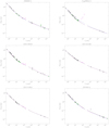 |
Fig. A.4 Observed and best-fit fluxes vs. wavelength for the O supergiants in our sample. Solid lines represent the best-fit model in the fixed-regions approach derived in this work (see Table 6 for parameters); magenta-dotted lines are either the best-fit solution (Adapted-regions approach; see Table 7 for parameters) or an alternate solution (see comments on individual objects in Section A.1); and blue-dashed lines correspond to existing previous best-fit models from P06. Magenta diamonds are our measured FIR fluxes at 70, 100 and 160 μm. Black squares and green circles indicate flux values from the literature. For those sources in common with P06, green circles indicate new available data added to the analysis. Arrows indicate upper limits. |
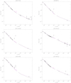 |
Fig. A.5 Observed and best-fit fluxes vs. wavelength for the B supergiants in our sample. Colours, symbols and line types as in Figure A.4. See comments on individual objects in Section A.2. |
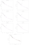 |
Fig. A.6 Same as Figure A.5, but displaying more B supergiants. See comments on individual objects in Section A.2. |
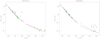 |
Fig. A.7 Observed and best-fit fluxes vs. wavelength for the two O giants in our sample, HD 24912 (ξ Per) and HD36861 (λ Ori A). Colours, symbols and line types as in Figure A.4, except for orange dashed-dotted lines, which indicate, for HD 24912, previous best-fit models from P06 (for HD 36861, the results from P06 are still indicated as magenta-dotted). See comments on individual objects in Section A.3. |
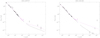 |
Fig. A.8 Observed and best-fit fluxes vs. wavelength for the OB dwarfs in our sample. Colours, symbols and line types as in Figure A.4. See comments on individual objects in Section A.4. |
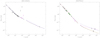 |
Fig. A.9 Observed and best-fit fluxes vs. wavelength for the two binary systems in our sample, HD 140494 (V973 Sco) and HD 37043 (ι Ori). Colours, symbols and line types as in Figure A.4, except that in the HD 149404 diagram, the blue-dashed line represents also an alternative solution, whereas for HD 37043, together with the orange dashed-dotted line, they represent the best-fit models by P06. See comments on individual objects in Section A.5. |
References
- Abbott, D. C. 1985, Astrophys. Space Sci. Lib., 116, 61 [NASA ADS] [CrossRef] [Google Scholar]
- Abbott, D. C., Bieging, J. H., & Churchwell, E. 1981, ApJ, 250, 645 [Google Scholar]
- Abbott, D. C., Telesco, C. M., & Wolff, S. C. 1984, ApJ, 279, 225 [NASA ADS] [CrossRef] [Google Scholar]
- Altenhoff, W. J., Thum, C., & Wendker, H. J. 1994, A&A, 281, 161 [NASA ADS] [Google Scholar]
- Anderson, L. S. 1985, ApJ, 298, 848 [NASA ADS] [CrossRef] [Google Scholar]
- Becker, R. H., & White, R. L. 1985, Astrophys. Space Sci. Lib., 116, 139 [NASA ADS] [CrossRef] [Google Scholar]
- Benaglia, P., Vink, J. S., Martí, J., et al. 2007, A&A, 467, 1265 [NASA ADS] [CrossRef] [EDP Sciences] [Google Scholar]
- Benedettini, M., Schisano, E., Pezzuto, S., et al. 2015, MNRAS, 453, 2036 [NASA ADS] [CrossRef] [Google Scholar]
- Berlanas, S. R., Herrero, A., Comerón, F., et al. 2018, A&A, 620, A56 [NASA ADS] [CrossRef] [EDP Sciences] [Google Scholar]
- Bieging, J. H., Abbott, D. C., & Churchwell, E. B. 1989, ApJ, 340, 518 [NASA ADS] [CrossRef] [Google Scholar]
- Björklund, R., Sundqvist, J. O., Puls, J., & Najarro, F. 2021, A&A, 648, A36 [EDP Sciences] [Google Scholar]
- Blomme, R., van de Steene, G. C., Prinja, R. K., Runacres, M. C., & Clark, J. S. 2003, A&A, 408, 715 [NASA ADS] [CrossRef] [EDP Sciences] [Google Scholar]
- Brott, I., de Mink, S. E., Cantiello, M., et al. 2011, A&A, 530, A115 [NASA ADS] [CrossRef] [EDP Sciences] [Google Scholar]
- Cantiello, M., Langer, N., Brott, I., et al. 2009, Commun. Asteroseismol., 158, 61 [NASA ADS] [Google Scholar]
- Cardelli, J. A., Clayton, G. C., & Mathis, J. S. 1989, ApJ, 345, 245 [Google Scholar]
- Carpay, J., de Jager, C., & Nieuwenhuijzen, H. 1991, A&A, 248, 475 [NASA ADS] [Google Scholar]
- Castor, J. I., Abbott, D. C., & Klein, R. I. 1975, ApJ, 195, 157 [Google Scholar]
- Chaldu, R., Honeycutt, R. K., & Penston, M. V. 1973, PASP, 85, 87 [NASA ADS] [CrossRef] [Google Scholar]
- Clark, J. S., Najarro, F., Negueruela, I., et al. 2012, A&A, 541, A145 [NASA ADS] [CrossRef] [EDP Sciences] [Google Scholar]
- Cohen, D. H., Leutenegger, M. A., Wollman, E. E., et al. 2010, MNRAS, 405, 2391 [NASA ADS] [Google Scholar]
- Contreras, M. E., Rodriguez, L. F., Gomez, Y., & Velazquez, A. 1996, ApJ, 469, 329 [NASA ADS] [CrossRef] [Google Scholar]
- Crowther, P. A., Lennon, D. J., & Walborn, N. R. 2006, A&A, 446, 279 [NASA ADS] [CrossRef] [EDP Sciences] [Google Scholar]
- Dessart, L., & Owocki, S. P. 2003, A&A, 406, L1 [NASA ADS] [CrossRef] [EDP Sciences] [Google Scholar]
- Dessart, L., & Owocki, S. P. 2005, A&A, 437, 657 [NASA ADS] [CrossRef] [EDP Sciences] [Google Scholar]
- Donati, J. F., Howarth, I. D., Jardine, M. M., et al. 2006, MNRAS, 370, 629 [NASA ADS] [CrossRef] [Google Scholar]
- Driessen, F. A., Sundqvist, J. O., & Kee, N. D. 2019, A&A, 631, A172 [NASA ADS] [CrossRef] [EDP Sciences] [Google Scholar]
- Ducati, J. R. 2002, VizieR Online Data Catalog: II/237 [NASA ADS] [Google Scholar]
- Ekström, S., Georgy, C., Eggenberger, P., et al. 2012, A&A, 537, A146 [Google Scholar]
- Feldmeier, A. 1995, A&A, 299, 523 [NASA ADS] [Google Scholar]
- Feldmeier, A., Puls, J., & Pauldrach, A. W. A. 1997, A&A, 322, 878 [NASA ADS] [Google Scholar]
- Friend, D. B., & Abbott, D. C. 1986, ApJ, 311, 701 [Google Scholar]
- Fullerton, A. W., Massa, D. L., & Prinja, R. K. 2006, ApJ, 637, 1025 [Google Scholar]
- Gaia Collaboration (Prusti, T., et al.) 2016, A&A, 595, A1 [NASA ADS] [CrossRef] [EDP Sciences] [Google Scholar]
- Gaia Collaboration (Brown, A. G. A., et al.) 2018, A&A, 616, A1 [NASA ADS] [CrossRef] [EDP Sciences] [Google Scholar]
- Gezari, D. Y., Arendt, R. G., Smith, R., et al. 2005, BAAS, 37, 1461 [NASA ADS] [Google Scholar]
- Gräfener, G., Koesterke, L., & Hamann, W.-R. 2002, A&A, 387, 244 [NASA ADS] [CrossRef] [EDP Sciences] [Google Scholar]
- Gutermuth, R. A., & Heyer, M. H. 2014, AAS Meeting Abs., 223, 336.05 [NASA ADS] [Google Scholar]
- Hamann, W.-R. 1981, A&A, 100, 169 [NASA ADS] [Google Scholar]
- Hamann, W.-R., Feldmeier, A., & Oskinova, L. M., eds. 2008, Clumping in Hot-star Winds (Postdam, Germany: Universität Postdam) [Google Scholar]
- Harris, D. H., Woolf, N. J., & Rieke, G. H. 1978, ApJ, 226, 829 [NASA ADS] [CrossRef] [Google Scholar]
- Haucke, M., Cidale, L. S., Venero, R. O. J., et al. 2018, A&A, 614, A91 [NASA ADS] [CrossRef] [EDP Sciences] [Google Scholar]
- Herrero, A., Puls, J., & Najarro, F. 2002, A&A, 396, 949 [NASA ADS] [CrossRef] [EDP Sciences] [Google Scholar]
- Hillier, D. J. 1987, ApJS, 63, 947 [NASA ADS] [CrossRef] [Google Scholar]
- Hillier, D. J. 2008, in Clumping in Hot-Star Winds, eds. W.-R. Hamann, A. Feldmeier, & L. M. Oskinova (Postdam, Germany: Universität Postdam), 93 [Google Scholar]
- Hillier, D. J., & Miller, D. L. 1998, ApJ, 496, 407 [NASA ADS] [CrossRef] [Google Scholar]
- Howarth, I. D., & Brown, A. 1991, IAU Symp., 143, 315 [Google Scholar]
- Jiang, Y.-F., Cantiello, M., Bildsten, L., Quataert, E., & Blaes, O. 2015, ApJ, 813, 74 [Google Scholar]
- Keszthelyi, Z., Puls, J., & Wade, G. A. 2017, A&A, 598, A4 [NASA ADS] [CrossRef] [EDP Sciences] [Google Scholar]
- Köhler, K., Langer, N., de Koter, A., et al. 2015, A&A, 573, A71 [NASA ADS] [CrossRef] [EDP Sciences] [Google Scholar]
- Kraus, M., Haucke, M., Cidale, L. S., et al. 2015, A&A, 581, A75 [NASA ADS] [CrossRef] [EDP Sciences] [Google Scholar]
- Kudritzki, R. P. 2002, ApJ, 577, 389 [NASA ADS] [CrossRef] [Google Scholar]
- Kurapati, S., Chandra, P., Wade, G., et al. 2017, MNRAS, 465, 2160 [NASA ADS] [CrossRef] [Google Scholar]
- Lamers, H. J. G. L. M., & Leitherer, C. 1993, ApJ, 412, 771 [Google Scholar]
- Lamers, H. J. G. L. M., & Waters, L. B. F. M. 1984, A&A, 136, 37 [NASA ADS] [Google Scholar]
- Lamers, H. J. G. L. M., Snow, T. P., & Lindholm, D. M. 1995, ApJ, 455, 269 [Google Scholar]
- Leitherer, C., & Robert, C. 1991, ApJ, 377, 629 [Google Scholar]
- Leitherer, C., & Wolf, B. 1982, Mitteilungen der Astronomischen Gesellschaft Hamburg, 55, 55 [NASA ADS] [Google Scholar]
- Leitherer, C., Chapman, J. M., & Koribalski, B. 1995, ApJ, 450, 289 [NASA ADS] [CrossRef] [Google Scholar]
- Li, H., Li, J.-Z., Yuan, J.-H., Huang, Y.-F., & Ren, Z.-Y. 2018, Res. Astron. Astrophys., 18, 122 [Google Scholar]
- Lopez, J. A., & Walsh, J. R. 1984, Rev. Mex. Astron. Astrofis., 9, 3 [NASA ADS] [Google Scholar]
- Lucy, L. B. 1971, ApJ, 163, 95 [Google Scholar]
- Lucy, L. B., & Solomon, P. M. 1970, ApJ, 159, 879 [Google Scholar]
- Luri, X., Brown, A. G. A., Sarro, L. M., et al. 2018, A&A, 616, A9 [NASA ADS] [CrossRef] [EDP Sciences] [Google Scholar]
- Marco, A., & Negueruela, I. 2009, A&A 493, 79 [NASA ADS] [CrossRef] [EDP Sciences] [Google Scholar]
- Markova, N., & Puls, J. 2008, A&A, 478, 823 [NASA ADS] [CrossRef] [EDP Sciences] [Google Scholar]
- Martins, F., & Palacios, A. 2013, A&A, 560, A16 [NASA ADS] [CrossRef] [EDP Sciences] [Google Scholar]
- Martins, F., Chené, A. N., Bouret, J. C., et al. 2019, A&A, 627, A170 [NASA ADS] [CrossRef] [EDP Sciences] [Google Scholar]
- Massey, P., & Thompson, A. B. 1991, AJ, 101, 1408 [NASA ADS] [CrossRef] [Google Scholar]
- Mokiem, M. R., de Koter, A., Puls, J., et al. 2005, A&A, 441, 711 [NASA ADS] [CrossRef] [EDP Sciences] [Google Scholar]
- Morel, T., Marchenko, S. V., Pati, A. K., et al. 2004, MNRAS, 351, 552 [NASA ADS] [CrossRef] [Google Scholar]
- Morford, J. C., Fenech, D. M., Prinja, R. K., Blomme, R., & Yates, J. A. 2016, MNRAS, 463, 763 [NASA ADS] [CrossRef] [Google Scholar]
- Morton, D. C., & Wright, A. E. 1978, MNRAS, 182, 47P [NASA ADS] [CrossRef] [Google Scholar]
- Morton, D. C., & Wright, A. E. 1979, IAU Symp., 83, 155 [NASA ADS] [Google Scholar]
- Najarro, F. 1995, PhD thesis, Ludwig-Maximilian University, Munich, Germany [Google Scholar]
- Najarro, F., & Figer, D. F. 1998, Ap&SS, 263, 251 [NASA ADS] [CrossRef] [Google Scholar]
- Najarro, F., Hillier, D. J., & Stahl, O. 1997, A&A, 326, 1117 [NASA ADS] [Google Scholar]
- Najarro, F., Puls, J., Herrero, A., et al. 2008, in Clumping in Hot-Star Winds, eds. W.-R. Hamann, A. Feldmeier, & L. M. Oskinova (Postdam, Germany: Universität Postdam), 43 [Google Scholar]
- Najarro, F., Hanson, M. M., & Puls, J. 2011, A&A, 535, A32 [NASA ADS] [CrossRef] [EDP Sciences] [Google Scholar]
- Nazé, Y., Rauw, G., Czesla, S., Mahy, L., & Campos, F. 2019, A&A, 627, A99 [NASA ADS] [CrossRef] [EDP Sciences] [Google Scholar]
- Ofek, E. O., & Frail, D. A. 2011, ApJ, 737, 45 [NASA ADS] [CrossRef] [Google Scholar]
- Oskinova, L. M., Hamann, W.-R., & Feldmeier, A. 2007, A&A, 476, 1331 [NASA ADS] [CrossRef] [EDP Sciences] [Google Scholar]
- Ott, S. 2010, ASP Conf. Ser., 434, 139 [Google Scholar]
- Owocki, S. P., Castor, J. I., & Rybicki, G. B. 1988, ApJ, 335, 914 [NASA ADS] [CrossRef] [Google Scholar]
- Owocki, S., Townsend, R., & Ud-Doula, A. 2008, Rev. Mex. Astron. Astrofis. Conf. Ser., 33, 80 [NASA ADS] [Google Scholar]
- Pablo, H., Richardson, N., Fuller, J., Moffat, A. F. J., & BEST and Ritter. 2017, IAU Symp., 329, 181 [NASA ADS] [Google Scholar]
- Panagia, N., & Felli, M. 1975, A&A, 39, 1 [Google Scholar]
- Pauldrach, A. W. A., & Puls, J. 1990, A&A, 237, 409 [NASA ADS] [Google Scholar]
- Pauldrach, A., Puls, J., & Kudritzki, R. P. 1986, A&A, 164, 86 [NASA ADS] [Google Scholar]
- Paulson, S. T., & Pandian, J. D. 2020, MNRAS, 492, 1335 [Google Scholar]
- Paxton, B., Bildsten, L., Dotter, A., et al. 2011, ApJS, 192, 3 [Google Scholar]
- Perrott, Y. C., Scaife, A. M. M., Green, D. A., et al. 2015, MNRAS, 453, 1396 [NASA ADS] [CrossRef] [Google Scholar]
- Petit, V., Owocki, S. P., Wade, G. A., et al. 2013, MNRAS, 429, 398 [NASA ADS] [CrossRef] [Google Scholar]
- Petrov, B., Vink, J. S., & Gräfener, G. 2014, A&A, 565, A62 [NASA ADS] [CrossRef] [EDP Sciences] [Google Scholar]
- Petrov, B., Vink, J. S., & Gräfener, G. 2016, MNRAS, 458, 1999 [NASA ADS] [CrossRef] [Google Scholar]
- Pilbratt, G. L., Riedinger, J. R., Passvogel, T., et al. 2010, A&A, 518, L1 [NASA ADS] [CrossRef] [EDP Sciences] [Google Scholar]
- Pittard, J. M., Stevens, I. R., Corcoran, M. F., et al. 2000, MNRAS, 319, 137 [Google Scholar]
- Poglitsch, A., Waelkens, C., Geis, N., et al. 2010, A&A, 518, L2 [NASA ADS] [CrossRef] [EDP Sciences] [Google Scholar]
- Puls, J., Kudritzki, R.-P., Herrero, A., et al. 1996, A&A, 305, 171 [NASA ADS] [Google Scholar]
- Puls, J., Repolust, T., Hoffmann, T. L., Jokuthy, A., & Venero, R. O. J. 2003, IAU Symp., 212, 61 [NASA ADS] [Google Scholar]
- Puls, J., Urbaneja, M. A., Venero, R., et al. 2005, A&A, 435, 669 [NASA ADS] [CrossRef] [EDP Sciences] [Google Scholar]
- Puls, J., Markova, N., Scuderi, S., et al. 2006, A&A, 454, 625 [NASA ADS] [CrossRef] [EDP Sciences] [Google Scholar]
- Puls, J., Vink, J. S., & Najarro, F. 2008, A&ARv, 16, 209 [NASA ADS] [CrossRef] [Google Scholar]
- Raucq, F., Rauw, G., Gosset, E., et al. 2016, A&A, 588, A10 [NASA ADS] [CrossRef] [EDP Sciences] [Google Scholar]
- Rauw, G., Nazé, Y., Carrier, F., et al. 2001, A&A, 368, 212 [NASA ADS] [CrossRef] [EDP Sciences] [Google Scholar]
- Repolust, T., Puls, J., Hanson, M. M., Kudritzki, R.-P., & Mokiem, M. R. 2005, A&A, 440, 261 [NASA ADS] [CrossRef] [EDP Sciences] [Google Scholar]
- Repolust, T., Puls, J., & Herrero, A. 2004, A&A, 415, 349 [NASA ADS] [CrossRef] [EDP Sciences] [Google Scholar]
- Rieke, G. H. 1974, ApJ, 193, L81 [NASA ADS] [CrossRef] [Google Scholar]
- Rieke, G. H., Lebofsky, M. J., & Low, F. J. 1985, AJ, 90, 900 [NASA ADS] [CrossRef] [Google Scholar]
- Runacres, M. C., & Owocki, S. P. 2002, A&A, 381, 1015 [NASA ADS] [CrossRef] [EDP Sciences] [Google Scholar]
- Runacres, M. C., & Owocki, S. P. 2005, A&A, 429, 323 [NASA ADS] [CrossRef] [EDP Sciences] [Google Scholar]
- Sahu, M., & Blaauw, A. 1993, ASP Conf. Ser., 35, 278 [NASA ADS] [Google Scholar]
- Sana, H., Gosset, E., Rauw, G., Sung, H., & Vreux, J.-M. 2006, A&A, 454, 1047 [NASA ADS] [CrossRef] [EDP Sciences] [Google Scholar]
- Sander, A. A. C. 2017, IAU Symp., 329, 215 [NASA ADS] [Google Scholar]
- Sander, A., Todt, H., Hainich, R., & Hamann, W. R. 2014, A&A, 563, A89 [NASA ADS] [CrossRef] [EDP Sciences] [Google Scholar]
- Sander, A. A. C., Hamann, W. R., Todt, H., Hainich, R., & Shenar, T. 2017, A&A, 603, A86 [NASA ADS] [CrossRef] [EDP Sciences] [Google Scholar]
- Santolaya-Rey, A. E., Puls, J., & Herrero, A. 1997, A&A, 323, 488 [NASA ADS] [Google Scholar]
- Schmutz, W. 1995, IAU Symp., 163, 127 [Google Scholar]
- Schnerr, R. S., Rygl, K. L. J., van der Horst, A. J., et al. 2007, A&A, 470, 1105 [NASA ADS] [CrossRef] [EDP Sciences] [Google Scholar]
- Scuderi, S., Panagia, N., Stanghellini, C., Trigilio, C., & Umana, G. 1998, A&A, 332, 251 [NASA ADS] [Google Scholar]
- Simón-Díaz, S., Herrero, A., Esteban, C., & Najarro, F. 2006, A&A, 448, 351 [NASA ADS] [CrossRef] [EDP Sciences] [Google Scholar]
- Sterken, C., de Groot, M., & van Genderen, A. M. 1997, A&A, 326, 640 [NASA ADS] [Google Scholar]
- Sundqvist, J. O., & Owocki, S. P. 2013, MNRAS, 428, 1837 [Google Scholar]
- Sundqvist, J. O., & Puls, J. 2018, A&A, 619, A59 [NASA ADS] [CrossRef] [EDP Sciences] [Google Scholar]
- Sundqvist, J. O., Puls, J., & Feldmeier, A. 2010, A&A, 510, A11 [NASA ADS] [CrossRef] [EDP Sciences] [Google Scholar]
- Sundqvist, J. O., Puls, J., Feldmeier, A., & Owocki, S. P. 2011, A&A, 528, A64 [NASA ADS] [CrossRef] [EDP Sciences] [Google Scholar]
- Sundqvist, J. O., Owocki, S. P., & Puls, J. 2018, A&A, 611, A17 [NASA ADS] [CrossRef] [EDP Sciences] [Google Scholar]
- Sundqvist, J. O., Björklund, R., Puls, J., & Najarro, F. 2019, A&A, 632, A126 [NASA ADS] [CrossRef] [EDP Sciences] [Google Scholar]
- Surlan, B., Hamann, W.-R., Aret, A., et al. 2013, A&A, 559, A130 [NASA ADS] [CrossRef] [EDP Sciences] [Google Scholar]
- Svoboda, B. E., Shirley, Y. L., Battersby, C., et al. 2016, ApJ, 822, 59 [Google Scholar]
- Torres-Dodgen, A. V., Carroll, M., & Tapia, M. 1991, MNRAS, 249, 1 [NASA ADS] [CrossRef] [Google Scholar]
- Traficante, A., Fuller, G. A., Pineda, J. E., & Pezzuto, S. 2015, A&A, 574, A119 [NASA ADS] [CrossRef] [EDP Sciences] [Google Scholar]
- Trigilio, C., Leto, P., Umana, G., Leone, F., & Buemi, C. S. 2004, A&A, 418, 593 [NASA ADS] [CrossRef] [EDP Sciences] [Google Scholar]
- ud-Doula, A., & Owocki, S. P. 2002, ApJ, 576, 413 [NASA ADS] [CrossRef] [Google Scholar]
- Urbaneja, M. A., Herrero, A., Bresolin, F., et al. 2003, ApJ, 584, L73 [Google Scholar]
- van den Oord, G. H. J., Lamers, H. J. G. L. M., Waters, L. B. F. M., Abbott, D. C., & Bieging, J. H. 1985, Astrophys. Space Sci. Lib., 116, 111 [NASA ADS] [CrossRef] [Google Scholar]
- van Loo, S., Runacres, M. C., & Blomme, R. 2005, A&A, 433, 313 [CrossRef] [EDP Sciences] [Google Scholar]
- Vink, J. S. 2018, A&A, 619, A54 [NASA ADS] [CrossRef] [EDP Sciences] [Google Scholar]
- Vink, J. S., de Koter, A., & Lamers, H. J. G. L. M. 2000, A&A, 362, 295 [Google Scholar]
- Vink, J. S., de Koter, A., & Lamers, H. J. G. L. M. 2001, A&A, 369, 574 [NASA ADS] [CrossRef] [EDP Sciences] [Google Scholar]
- Vink, J. S., Brott, I., Gräfener, G., et al. 2010, A&A, 512, L7 [NASA ADS] [CrossRef] [EDP Sciences] [Google Scholar]
- Waldron, W. L., Corcoran, M. F., Drake, S. A., & Smale, A. P. 1998, ApJS, 118, 217 [CrossRef] [Google Scholar]
- Wendker, H. J., & Altenhoff, W. J. 1980, A&A, 92, L5 [NASA ADS] [Google Scholar]
- White, R. L., & Becker, R. H. 1983, ApJ, 272, L19 [CrossRef] [Google Scholar]
- Whittet, D. C. B., & van Breda, I. G. 1980, MNRAS, 192, 467 [NASA ADS] [CrossRef] [Google Scholar]
- Wright, A. E., & Barlow, M. J. 1975, MNRAS, 170, 41 [Google Scholar]
- Yusof, N., Hirschi, R., Meynet, G., et al. 2013, MNRAS, 433, 1114 [NASA ADS] [CrossRef] [Google Scholar]
Some current atmosphere models account, among other physics (Hillier 1987), for X-ray emission (Feldmeier et al. 1997), line-blanketing effects (Anderson 1985), and clumping using various parameterisations (Najarro et al. 2008; Sundqvist & Puls 2018).
Periods in the variability of the photospheric lines from 2.7 h to 22.5 days related to pulsation activity have been recently reported Kraus et al. (2015).
Recent Gaia Early DR3 parallax estimates for Cyg OB2#12 relocated the star within its stellar association, at ~1.78 kpc. For the rest of our sample DR3 parallaxes are similar to Gaia DR2 measurements, except for HD 210839 and HD 36861, whose new distances are a factor 1.4 larger than implied from Gaia DR2 (see discussion in Sect. 3).
40% is the largest variation in distance between Gaia DR2 and early DR3 measurements for our sample, see Sect. 2.4.
Current evolutionary models implement Vink’s equations in several ways. For a brief summary see e.g. Martins & Palacios (2013) and Keszthelyi et al. (2017).


The difference between the flux observations at 6 cm is not large enough to consider HD 30614 a variable source (Scuderi et al. 1998).
Although CygOB2#12 has been classified as eBHG due to its similarities to other eBHGs, the combination of its extremely high L* and low Teff cannot be consistently reproduced by any theoretical isochrones (Clark et al. 2012). Thus, its evolutionary stage remains unclear.
All Tables
List of the OB stars observed with Herschel-PACS (IP: OT1_mrubio_1/OT2_mrubio_2) and the photometric data compiled from the literature used in this work (see references below).
Final used distances and associated errors, reddening parameters and derived stellar radii.
Defined wind region boundaries and the corresponding clumping factors used in this work.
Sample of analysed OB stars in this work and the initial set of stellar and wind parameters from the literature (‘ref’ column) used as input values in our simulations. log g indicates gravities without centrifugal correction.
Maximum mass-loss rates, minimum clumping factors and alternative boundaries of the defined wind regions (adapted-regions approach, see Sect. 3) providing the best-fit models for some objects in the sample.
Clumping factors and maximum mass-loss rates (in units of 10−6M⊙ yr−1) derived for alternative values (β1 and β2) of the used β in our simulations in the fixed-regions approach.
Minimum clumping structure and Ṁmax of HD 198474 derived in this work for the interval of stellar parameters provided by Markova & Puls (2008) (see text and Figure A.2).
All Figures
|
Fig. 1 From left to right: PACS 70 μm miniscan maps taken at position angles 70° and 110°, and the final composed image of the O supergiant star HD 66811 (ζ Pup). |
| In the text | |
|
Fig. 2 Schematic of the wind emission: different wind regions as a function of the spectral range and their corresponding radial distance to the photosphere (r), as defined in Table 4. The emission model corresponds to the unclumped stellar wind of a O supergiant star (Teff = 33 kK, Ṁ = 8.6 × 10⁻⁶ M⊙ yr−1). |
| In the text | |
|
Fig. 3 From top to bottom: observed and best-fit fluxes vs. wavelength in the fixed-regions approach for HD 151804, HD 193237 (P Cyg), and HD 24398 (ζ Per). Solid lines correspond to the best-fits; magenta-dotted, blue-dashed and orange-dashed-dotted lines correspond to different models (see text). |
| In the text | |
|
Fig. 4 Derived invariant log Q′ = log (Ṁmax/R*1.5) for our sample as a function of spectral type, in units of M⊙ yr−1 R⊙−1.5. Different symbols and colours represent the luminosity class coverage in the sample and the nature of the sources, respectively. Arrows indicate objects with upper limits for Ṁmax, and symbols joined by dashed-lines correspond to sources with two possible solutions for Ṁmax. |
| In the text | |
|
Fig. 5 From top to bottom: clumping factor ratio |
| In the text | |
|
Fig. 6 Top: individual minimum and average values of the clumping factors for r ≥ 2 R* derived in the fixed-regions approach for the sub-sample of O (left) and B (right) supergiants (see Sect. 4.2). Bottom: average minimum clumping stratification of the sub-sample as in the top panel, with error bars. Solid error bars correspond to the standard deviation of ⟨
|
| In the text | |
|
Fig. 7 Absolute ratio between the semi-widths (δβ+, δβ−) of the validity interval of β as a function of spectral type for the best-fit solutions derived in the fixed-regions approach in this work (see Table 6). Symbols and colours as in Fig. 4. The circled symbol indicates that the ratio was divided by 3 for display purposes. |
| In the text | |
|
Fig. 8 Fromtop to bottom, empirical to theoretical mass-loss rates ratio, in logarithmic scale, as a function of effective temperature for the OB supergiants sub-sample. Empirical mass-loss rates correspond to the Ṁmax derived in this work. Theoretical mass-loss rates, |
| In the text | |
|
Fig. 9 Top: empirical-maximum (Ṁmax) and theoretical ( |
| In the text | |
|
Fig. A.1 Comparison between the best-fit solutions for HD 210839 by P06 (blue-dashed and orange-dotted-dashed lines) and our best-fit solutions (solid and magenta-dotted lines) for the same value of the distance (see text). Magenta diamonds are our measured FIR fluxes at 70, 100 and 160 μm. Black squares and green circles indicate flux values from the literature. For those sources in common with P06, green circles indicate new available data added to the analysis. Arrows indicate upper limits. |
| In the text | |
|
Fig. A.2 Observed and best-fit fluxes vs. wavelength for HD 198478 depending on the input parameters used in the simulations (see Table A.1 and text in Appendix A.2). Colours and symbols as in Figure A.1. Left: Best-fit models 470 kms−1 for YHe = 0.2 (solid line; Sol. 1a) and YHe = 0.1 (magenta-dotted line; Sol. 1b). Right: Best-fit models for υ∞ = 200 kms−1 for YHe = 0.2 (solid line; Sol. 2a) and YHe = 0.1 (magenta-dotted line; Sol. 2b). The blue-dashed line in both plots shows how changes in YHe are reflected in the emission flux model. |
| In the text | |
|
Fig. A.3 Comparison between the best-fit solutions for HD 24912 (ξ Per) by P06(solid and magenta lines, see text) and our flux estimates at 70, 100 and 160 μm (magenta diamonds). Colours and symbols as in Figure A.1. |
| In the text | |
|
Fig. A.4 Observed and best-fit fluxes vs. wavelength for the O supergiants in our sample. Solid lines represent the best-fit model in the fixed-regions approach derived in this work (see Table 6 for parameters); magenta-dotted lines are either the best-fit solution (Adapted-regions approach; see Table 7 for parameters) or an alternate solution (see comments on individual objects in Section A.1); and blue-dashed lines correspond to existing previous best-fit models from P06. Magenta diamonds are our measured FIR fluxes at 70, 100 and 160 μm. Black squares and green circles indicate flux values from the literature. For those sources in common with P06, green circles indicate new available data added to the analysis. Arrows indicate upper limits. |
| In the text | |
|
Fig. A.5 Observed and best-fit fluxes vs. wavelength for the B supergiants in our sample. Colours, symbols and line types as in Figure A.4. See comments on individual objects in Section A.2. |
| In the text | |
|
Fig. A.6 Same as Figure A.5, but displaying more B supergiants. See comments on individual objects in Section A.2. |
| In the text | |
|
Fig. A.7 Observed and best-fit fluxes vs. wavelength for the two O giants in our sample, HD 24912 (ξ Per) and HD36861 (λ Ori A). Colours, symbols and line types as in Figure A.4, except for orange dashed-dotted lines, which indicate, for HD 24912, previous best-fit models from P06 (for HD 36861, the results from P06 are still indicated as magenta-dotted). See comments on individual objects in Section A.3. |
| In the text | |
|
Fig. A.8 Observed and best-fit fluxes vs. wavelength for the OB dwarfs in our sample. Colours, symbols and line types as in Figure A.4. See comments on individual objects in Section A.4. |
| In the text | |
|
Fig. A.9 Observed and best-fit fluxes vs. wavelength for the two binary systems in our sample, HD 140494 (V973 Sco) and HD 37043 (ι Ori). Colours, symbols and line types as in Figure A.4, except that in the HD 149404 diagram, the blue-dashed line represents also an alternative solution, whereas for HD 37043, together with the orange dashed-dotted line, they represent the best-fit models by P06. See comments on individual objects in Section A.5. |
| In the text | |
Current usage metrics show cumulative count of Article Views (full-text article views including HTML views, PDF and ePub downloads, according to the available data) and Abstracts Views on Vision4Press platform.
Data correspond to usage on the plateform after 2015. The current usage metrics is available 48-96 hours after online publication and is updated daily on week days.
Initial download of the metrics may take a while.