| Issue |
A&A
Volume 657, January 2022
|
|
|---|---|---|
| Article Number | A11 | |
| Number of page(s) | 19 | |
| Section | Stellar structure and evolution | |
| DOI | https://doi.org/10.1051/0004-6361/202141182 | |
| Published online | 21 December 2021 | |
Clues on jet behavior from simultaneous radio-X-ray fits of GX 339-4
1
Univ. Grenoble Alpes, CNRS, IPAG, 38000 Grenoble, France
e-mail: This email address is being protected from spambots. You need JavaScript enabled to view it.
2
Villanova University, Department of Physics, Villanova, PA 19085, USA
3
Institute of Astronomy, University of Cambridge, Madingley Road, Cambridge CB3 OHA, UK
4
IRAP, Université de toulouse, CNRS, UPS, CNES, Toulouse, France
5
AIM, CEA, CNRS, Université de Paris, Université Paris-Saclay, 91191 Gif-sur-Yvette, France
6
Station de Radioastronomie de Nançay, Observatoire de Paris, PSL Research University, CNRS, Univ. Orléans, 18330 Nançay, France
Received:
26
April
2021
Accepted:
13
July
2021
Abstract
Understanding the mechanisms of accretion-ejection during X-ray binary (XrB) outbursts has been a problem for several decades. For instance, it is still not clear what controls the spectral evolution of these objects from the hard to the soft states and then back to the hard states at the end of the outburst, tracing the well-known hysteresis cycle in the hardness-intensity diagram. Moreover, the link between the spectral states and the presence or absence of radio emission is still highly debated. In a series of papers we developed a model composed of a truncated outer standard accretion disk (SAD, from the solution of Shakura and Sunyaev) and an inner jet emitting disk (JED). In this paradigm, the JED plays the role of the hot corona while simultaneously explaining the presence of a radio jet. Our goal is to apply for the first time direct fitting procedures of the JED-SAD model to the hard states of four outbursts of GX 339-4 observed during the 2000–2010 decade by RXTE, combined with simultaneous or quasi simultaneous ATCA observations. We built JED-SAD model tables usable in XSPEC, as well as a reflection model table based on the XILLVER model of XSPEC. We applied our model to the 452 hard state observations obtained with RXTE/PCA. We were able to correctly fit the X-ray spectra and simultaneously reproduce the radio flux with an accuracy better than 15%. We show that the functional dependency of the radio emission on the model parameters (mainly the accretion rate and the transition radius between the JED and the SAD) is similar for all the rising phases of the different outbursts of GX 339-4, but it is significantly different from the functional dependency obtained in the decaying phases. This result strongly suggests a change in the radiative and/or dynamical properties of the ejection between the beginning and the end of the outburst. We discuss possible scenarios that could explain these differences.
Key words: black hole physics / X-rays: binaries / accretion / accretion disks / ISM: jets and outflows
© S. Barnier et al. 2021
 Open Access article, published by EDP Sciences, under the terms of the Creative Commons Attribution License (https://creativecommons.org/licenses/by/4.0), which permits unrestricted use, distribution, and reproduction in any medium, provided the original work is properly cited.
1. Introduction
X-ray binaries (XrBs) are formidable laboratories for the study of the accretion-ejection processes around compact objects. Most of the time in a quiescent state they can suddenly enter an outburst that can last from a few months to a year, increasing their overall luminosity by several orders of magnitude. The X-ray emission is commonly believed to be produced by the inner regions of the accretion flow, whereas the radio emission is thought to originate from relativistic jets. Simultaneously with the X-ray spectral evolution along the outburst (from hard to soft states; e.g., Remillard & McClintock 2006; Done et al. 2007), the radio emission switches from jet-dominated states during the hard X-ray states, at the beginning and the end of the outburst, to jet-quenched states during the soft X-ray states, in the central part of the outburst (e.g., Corbel et al. 2004; Fender & Belloni 2004). These outbursts are usually represented in the so-called hardness-intensity diagram (HID) where they follow a typical “q” shape (see, e.g., Dunn et al. 2010).
A physical understanding has yet to be found to explain the complete behavior of these outbursts, even if a few points have reached consensus. For instance, the start of the outburst is believed to originate from disk instabilities in the outer regions of the accretion flow, driven by the ionization of hydrogen above a critical temperature (e.g., Hameury et al. 1998; Frank et al. 2002). The nature of the soft state X-ray emission, peaking in the soft X-rays, is commonly attributed to the presence of an accretion disk, down to the Innermost Stable Circular Orbit (ISCO), and the standard accretion disk model (SAD, Shakura & Sunyaev 1973) seems to describe the observed radiative output reasonably well. The exact nature of the hard X-ray emitting region, the hot corona, is however less clear. Given its intense luminosity, it is expected to be located close to the black hole where the release of gravitational power is the largest. The variability of the source is consistent with a very compact region (De Marco et al. 2017), but the exact geometry is still a matter of debate. It could be located somewhere above the black hole (the so-called lamppost geometry, e.g., Matt et al. 1991; Martocchia & Matt 1996; Miniutti & Fabian 2004). It can also partly cover the accretion disk (the patchy corona geometry, e.g., Haardt et al. 1997) or it can fill the inner part of the accretion flow, the accretion disk being present in the outer part of the flow (the corona-truncated disk geometry, e.g., Esin et al. 1997). The hot corona is most probably a combination of all these geometries; it could even evolve from one geometry to the other depending on the state of the source.
The dominant radiative process producing the hard X-rays is generally believed to be external Comptonization, meaning Comptonization of the external UV and soft X-ray photons produced by the accretion disk off the hot electrons present in the corona. These electrons are generally supposed to follow a relativistic thermal distribution to explain the presence of a high-energy cutoff, generally observed in the brightest hard states (see, e.g., Fabian et al. 2017 for a recent compilation). While the release of the gravitation power is undoubtedly the source of the corona heating, how this heating is transferred to the particles and how particles reach thermal equilibrium is still not understood. The magnetic field is expected to play a major role (e.g., Merloni & Fabian 2001), but the details of the process are unknown. The correlation between X-ray emission (from the corona) and radio emission (from the jet) (e.g., Gallo et al. 2003, 2012; Corbel et al. 2000, 2003, 2013; Coriat et al. 2011) also indicates a strong link between accretion and ejection, supporting the presence of a magnetic field in the disk.
Models of the hot corona commonly used in the literature are generally oversimplified. The geometry is assumed to have a basic shape, for instance spherical, slab, or even point-like. Its temperature and density are supposed to be uniform across the corona. External Comptonization is usually the unique radiative process taken into account and the spectral emission is often approximated by a cutoff power law (or similar) shape. Most of the time no physically motivated configuration or comparison with numerical simulations of this simplified model is proposed. More importantly, the jet emission and its impact on the accretion system is generally entirely ignored.
Magnetized accretion-ejection solutions that self-consistently treat both the accretion disk and the jets have been in development for more than 20 years (Ferreira & Pelletier 1995; Ferreira 1997) and have since been validated through numerical simulations (e.g., Zanni et al. 2007, Jacquemin-Ide et al. 2021). In these works the accretion disk is assumed to be threaded by a large-scale magnetic field. In the regions where the magnetization μ(r) = Pmag/Ptot is on the order of unity (with Pmag the magnetic pressure and Ptot the total pressure, i.e., the sum of the thermal and radiation pressure), the magnetic hoop stress overcomes both the outflow pressure gradient and the centrifugal forces, and self-confined non-relativistic jets can be produced. In these conditions the accretion disk is called a jet emitting disk (JED). The effect of the jets on the disk structure can be tremendous since the jets’ torque can efficiently extract the disk angular momentum, significantly increasing the accretion speed. Consequently, for a given accretion rate, a JED has a much lower density in comparison to the standard accretion disk (e.g., Ferreira et al. 2006). The parameter space for stationary JED solutions corresponds to magnetization μ in the range [0.1,1], small ejection index p < 0.1 defined by ṁ(r) ∝ rp (with ṁ the mass accretion rate measured at a given radius r), large sonic mach number ms = ur/cs in the range Arnaud (1996), Begelman & Armitage (2014), Bel et al. (2011) (with ur the accretion speed and cs the local speed of sound), and jet power fraction b = Pjets/Pacc between 0.1 and almost 1 for very thin JED (Ferreira 1997), where Pjets is the power feeding the jets and Pacc the total gravitational power released by the accretion flow within the JED. We note that for weak magnetization (μ ≪ 0.1), no collimation occurs and uncollimated winds are produced. The accretion disk structure is then not very different from the standard solution (e.g., Jacquemin-Ide et al. 2019).
Ferreira et al. (2006) proposed a hybrid disk paradigm to address the full accretion-ejection evolution of XrBs in outbursts (see also Petrucci et al. 2008). The accretion disk is threaded by a vertical magnetic field and extends all the way down to the innermost circular orbit. The outer part of the flow has a low magnetization, resulting in an outer SAD. On the contrary, the inner part has an important mid-plane magnetization and the accretion flow has a JED structure. This radial distribution of the magnetization appears to be a natural outcome of the presence of large-scale magnetic fields in the accretion flow, the magnetic flux accumulating toward the center to produce a magnetized disk with a fast accretion timescale (Scepi et al. 2020, Jacquemin-Ide et al. 2021).
Marcel et al. (2018a) developed a two-temperature plasma code to compute the spectral energy distribution (SED) of any JED-SAD configuration. In addition to the parameter μ, p, ms, and b that characterizes a JED solution, the output SED also depends on the transition radius rJ (in units of gravitational radius RG = GM/c2) between the JED and the SAD, as well as the mass accretion rate ṁin (in units of Eddington accretion mass rate ṀEdd = LEdd/c2) reaching the ISCO.
In our view, rJ and ṁin are expected to be physically linked through the evolution the magnetization across the accretion flow, dividing it in an inner strongly magnetized part (the JED) and an outer weakly magnetized one (the SAD). This link is far from being trivial to estimate and requires global 3D MHD simulations, which is far beyond of the scope of our present modeling, to catch it. In the absence of any physical law that could be used as an input, we consider the parameters rJ and ṁin to be independent parameters.
Varying rJ and ṁin, Marcel et al. (2018a) showed that the JED-SAD model was able to qualitatively reproduce the spectral evolution of an entire outburst. The JED radiative properties agree with the X-ray emission observed in compact objects (Petrucci et al. 2010; Marcel et al. 2018b,a), meaning that the JED can play the role of the hard X-ray emitting hot corona. At the beginning of the outburst the disk is characterized by a low-luminosity hard component that can be represented by a JED with large radial extend (rJ ≫ 1), while the mass accretion rate ṁin is low (ṁin < 0.1). During the rising part of the outburst the luminosity increases, thus the mass accretion rate increases, but rJ is still several times the ISCO radius. While transitioning to the soft states, rJ starts to decrease until the complete disappearance of the JED when rJ ∼ rISCO. This coincides with the disappearance of the radio emission (no more JED implies no more jets). During the soft states, the disk is dominated by the thermal component of the SAD and rJ stays equal to rISCO. Eventually, during the decaying phase of the outburst, a JED reappears when the system transitions back to the hard state, ṁin decreases, rJ increases again, and the system returns to the hybrid JED-SAD configuration. With the following decrease in the accretion rate, the XrB then fades to the quiescent state.
Marcel et al. (2019) (hereafter M19) performed the first application of the JED-SAD model to real data by qualitatively reproducing the spectral evolution of GX 339-4 during the 2010 outburst observed by RXTE. A similar study has been recently extended to three other outbursts of GX 339-4 (Marcel et al. 2020, hereafter M20). These authors did not directly fit the data given the large number of observations as well as the lack of a consistent reflection model component. Instead, they produced a large grid of spectra for a set of parameters (rJ, ṁin) and fitted each simulated spectrum with a disk plus power law (disk + power law) model. This provided spectral characteristics (disk flux, power law luminosity fraction, X-ray spectral index) that were then compared to the best fit results obtained by fitting the RXTE/PCA data with a similar disk + power law model (Clavel et al. 2016). This procedure allowed us to derive the qualitative evolution of rJ and ṁin that reproduces JED-SAD spectra with the closest spectral characteristics to the observed ones.
An important output of the JED-SAD model is the estimate of the jet’s power in a consistent way with the JED structure. The radio signature produced by this jet is less straightforward to estimate, however, since it depends on the detailed treatment of the jet particle emission all along the jet. Following Heinz & Sunyaev (2003) (hereafter HS03), M19 proposed an expression for the radio flux produced at a radio frequency νR by a jet launched from a JED characterized by rJ and ṁin :
 (1)
(1)
Here  is a scaling factor and FEdd = LEdd/4πd2 the Eddington flux. Equation (1) has the same dependency with the accretion rate as in the self-similar approach of HS03, but there is an additional multiplicative term (rJ − risco)5/6 that reflects the necessarily finite radial dimension of the jet due to the finite radial dimension of the JED (see discussion in M19). By trying to simultaneously reproduce the X-ray and radio emission, M19 were able to put constraints on ṁin, rJ, and
  in the case of GX 339-4, assuming a constant
  for all the outbursts1.
The present paper aims to make a step forward in the comparison of the JED-SAD model to real data through a direct fitting procedure of simultaneous radio and X-ray data of an X-ray binary. The improvements compared to the previous works are twofold. First we added a consistent reflection component in the model and second we obtained more reliable and precise constraints on our model parameters (rJ and ṁin). To do so, we developed the required tools to apply our JED-SAD model to standard fitting software (e.g., XSPEC, Arnaud 1996).
We focus in this paper on the simultaneous radio–X-ray coverage of the XrB GX 339-4 during the lifetime of the RXTE satellite (1995–2012). This corresponds to four major outbursts starting in 2002, 2004, 2007, and 2010. The data selection is discussed more precisely in Sect. 2. Our fitting procedure and first fit results, using Eq. (1) for the radio emission, are discussed in Sect. 3. These results suggest, however, a different functional dependency of the radio emission with rJ and ṁin compared to Eq. (1). A deeper analysis of the radio behavior is then performed in Sect. 4 and supports two different functional behaviors of the radio emission between the beginning and the end of the outburst. The implications of these results are discussed in Sect. 5, and we conclude in Sect. 6.
2. Data selection
To test our JED-SAD paradigm we focused on simultaneous or quasi-simultaneous radio–X-ray observations of GX 339-4. We only used pure hard states (i.e., those at the very right part of the HID), either in the rising or decaying phase, and did not include the transition phases of the outburst even when radio emission was detected (during the so-called hard intermediate state, HIS). The reasons for this choice are twofold. First, the radio flux evolves smoothly during pure hard states, a signature of stationary processes hopefully easier to catch. Conversely, an important radio variability is observed during the transition phases, especially during the hard-to-soft transition. Second, during the transition states, the hard-tail component progressively appears. As this component is not well understood and is not self-consistently included in the JED-SAD model, we did not select the transition states.
We selected X-ray spectra from the RXTE-PCA archive of GX 339-4 during the 2000–2010 decade. In order to have a uniform data analysis, we did not include the data from the RXTE-HEXTE instrument since they were not always usable (e.g., in the case of low flux observations or after March 2010 when it stopped observing). The data processing is detailed in Clavel et al. (2016). Since the instrumental background was generally found to be on the order of, or larger than, the source emission above 25 keV, we limited our spectral analysis to the 3–25 keV energy range of the PCA instrument. We plot the 2000–2010 PCA X-ray light curve of GX 339-4 in Fig. 1. During this period, GX 339-4 underwent four complete outbursts, in 2002, 2004, 2007, and 2010, hereafter outbursts 1, 2, 3, and 4. The hard-only or failed outbursts of 2006 and 2008 were not selected for this study2 since they may be intrinsically different from the ones accomplishing an entire HID. We follow Clavel et al. (2016) for the definition of the hard-state periods of each outburst. We list in Table 1 the corresponding starting and ending Modified Julian Dates (MJD) of both the rising and the decaying hard-state phases.
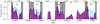 |
Fig. 1. GX 339-4 X-ray light curve in the 3–200 keV energy band of the 2000–2010 decade obtained with the Clavel et al. (2016) fits. The violet filled region shows the power law unabsorbed flux, while the cyan region represents the disk unabsorbed flux. The selected spectra for this study are highlighted in gray: the rising and decaying hard states of the four outbursts (1, 2, 3, and 4). At the top the red lines represent the date when steady radio fluxes were observed at 9 GHz (from Corbel et al. 2013). |
Hard-state periods of the four outbursts and number of selected observations.
In radio we used the 9 GHz fluxes obtained with the Australia Telescope Compact Array (ATCA) and discussed in Corbel et al. (2013)3. Compared to the X-ray observations, the radio survey is quite sparse (see Fig. 1), so we selected only the radio fluxes close to X-ray pointings by less than one day (which we call quasi-simultaneous radio–X-ray observations).
This selection corresponds to a total of 452 hard X-ray spectra and 57 radio fluxes distributed among the four outbursts. Outburst 4 is the one with the best X-ray and radio coverage, with about 80 X-ray spectra and 24 radio measurements that are evenly distributed along the outburst. Thanks to this large radio coverage we chose to linearly interpolate the radio light curve to estimate the radio fluxes for each of the 80 X-ray spectra of this outburst. This is supported by the smooth evolution of the radio light curve during the pure hard states. The resulting interpolation is plotted in Fig. A.1. This interpolation was not possible for the other outbursts, due to the insufficient number of radio pointings.
3. X-ray and radio fits
3.1. Methodology
Similarly to M19, we assume a distance d = 8 kpc for GX 339-4 (Zdziarski et al. 2004, 2019; Parker et al. 2016). The black hole mass is estimated between 4 and 11 M⊙ (Parker et al. 2016; Zdziarski et al. 2019), and we assume a black hole mass of 10 M⊙. The innermost stable circular orbit risco was assumed equal to 2 in Rg units. This is equivalent to a black hole spin of 0.94 (Miller et al. 2008; García et al. 2015). Finally, for the Galactic hydrogen column density we used 0.6 × 1022 cm−2 (Zdziarski et al. 2004; Bel et al. 2011).
In the JED-SAD model the two parameters left free to vary during the fitting procedure are rJ and ṁin. All the other parameters of the JED-SAD (see Sect. 1) were set to the same values as in M19: b = 0.3, ms = 1.5, and p = 0.014.
We created XSPEC model tables for the JED and the SAD components separately with 40 values of ṁin and 25 values of rJ logarithmicaly distributed in the range [0.001,10] and [1,300], respectively. We also produced a reflection table. For this purpose, we used the XILLVER reflection model (Garcia et al. 2013). For each couple (rJ, ṁin) of the JED table, we fitted the corresponding JED spectrum with a cutoff power law model. This fit provides a spectral index and a high-energy cutoff, which we injected in the XILLVER table to produce different reflection spectra for different values of the disk ionization log(ξ) and iron abundance A(Fe) (in solar units). The disk inclination was set to 30°, an inclination consistent with the value expected for GX 339-4 (Parker et al. 2016). The resulting table thus possesses five different parameters for each spectrum: the two JED-SAD parameters (rJ, ṁin), and the three reflection parameters log(ξ), A(Fe), and the reflection normalization.
We then used an automatic fitting procedure using the pyxspec library (a python interface to XSPEC). We fit the X-ray spectra with the following XSPEC model: tbabs * (atable(JEDtable) + atable(SADtable) + kdblur*atable(Refltable)). Here JEDtable, SADtable, and Refltable are the XSPEC tables for the JED, SAD, and reflection spectra, respectively, and KDBLUR is a convolution model of XSPEC to take into account the relativistic effects from the accretion disk around a rotating black hole (according to the original calculations by Laor 1991). The parameters rJ and ṁin are linked between the tables and we set the inner radius of KDBLUR to the inner radius of the SAD (i.e., rJ). In KDBLUR, we set the index of the disk emissivity to 3 (its default value), the outer disk radius to 400 Rg, and the inclination to 30°.
3.2. X-ray fits
Using the fitting procedure described above, we obtained the best fit values for rJ and ṁin for each X-ray observation in our sample. The iron abundance values are clustered around seven times the solar abundance, in agreement with similar spectral analysis of GX 339-4 (e.g., García et al. 2015; Fürst et al. 2015; Parker et al. 2016; Wang-Ji et al. 2018), and we set it to this value in the following5. As examples, we show in Fig. 2 a few of our X-ray best fits obtained for different observations distributed in the hard X-ray states of outburst 4. In the top left panel of this figure we represent the HID as well as the hard states (blue diamond) that we fit. We also highlight the five observations whose spectral fits are presented in the other panels of the figure.
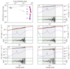 |
Fig. 2. Best fits of some observations of outburst 4. Top left: hardness intensity diagram of outburst 4. The blue diamond shows the hard state used for this outburst. The five red points are the five observations plotted in the different figures from a to e. a–e: best fit spectra and the data/model ratio for the five observations indicated in red in the HID. The gray region shows the PCA energy range used for the fit. The data are in black and the best fit model in gray; the JED spectrum is in red, the SAD spectrum in green, and the reflection component in blue. The best fit parameters for each observation are listed in Table 2. |
During the rising phase (observations a, b, and c), the high-energy cutoff slowly appears in the model with the rise in luminosity6. At the same time, the iron line changes shape under the influence of both the evolution of the disk ionization parameter and the black hole gravity as the transition radius rJ decreases (general relativity effects). During the decaying phase (observations d and e), as the luminosity decreases, the standard accretion disk component disappears with the increase in rJ.
The evolutions of rJ and ṁin for our entire data sample are shown in Fig. 3; the left panel shows the light curves of rJ and the right panel those of ṁin. We divided each panel into two parts, showing the rising phase first and then the decaying phase. The large green region represents the area where the minimization function used by M19 to constrain rJ and ṁin varies by less than 10% with respect to its minimum. The blue points with black error bars and connected by dashed lines represent the results of this paper obtained by fitting the X-ray spectra in XSPEC.
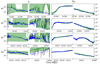 |
Fig. 3. Results of the fitting procedure. Left: transition radius rJ (from risco to 300) between the JED and the SAD. Right: mass accretion rate ṁin. Each side is divided vertically between the four outbursts and horizontally between the rising and decaying phase of each outburst. The green solid line represent the results from M19 and M20, and the green region indicates where the minimization function varies by less than 10% with respect to its minimum. The blue dashed line shows the results of the fitting procedure and the black vertical bar the associated 90% confidence range. The decaying phase of outburst 4 is the subject of Appendix B. |
We obtained much tighter constraints compared to M19, especially for rJ during the rising phase. There are two reasons for this. First, M19 did not directly fit the data, their main objectives being to qualitatively reproduce the outburst spectral and flux evolution. Second, M19 did not use a χ2 statistic to constrain their parameters because the χ2 statistic is not well adapted to their methodology.
Nevertheless, the constraints obtained with our fitting procedure are almost always embedded within the green area obtained by M19, which shows the good agreement between the two approaches. This is noticeably the case for ṁin, which is well constrained in the two methods and are in very good agreement with each other. Interestingly, our values for rJ are apparently better constrained in the rising phase of the outbursts, its behavior being more erratic and with larger error bars in the decaying phase. This could be a natural effect of the decrease in the data statistics when the flux decreases, but this trend is not observed for ṁin. This instead suggests that our JED-SAD spectra are less dependent on rJ at low accretion rates.
It should be noted that the χ2 space does not always follow a Gaussian shape (see Fig. B.2) and the error bars should not be taken as sigma errors, but instead as lower and upper limits with a 90% confidence. Thus, none of the pure hard states are consistent with risco, and a JED is always required in the fit.
The evolution of rJ during the decaying phase of outburst 4 is the subject of Appendix B where we detail how we obtained the presented values of rJ using a maximum likelihood method. When a small rJ solution was found in the automatic procedure (rJ < 10), we checked the parameter space for a statistically equivalent solution for a larger value of rJ. Whenever such a solution was found, we selected it (see Appendix B). The motivations for this choice are twofold: higher values of rJ are observed in the decaying phase of the other outbursts (see Fig. 3, outbursts 2 and 3) and the resulting increase in rJ when going to quiescence is consistent with the JED-SAD dynamical picture.
3.3. Taking into account the radio emission
We now reproduce the radio fluxes using Eq. (1) to model the radio emission. Since the radio survey is generally quite sparse, we first concentrate on the rising phase of outburst 4, where the radio coverage is sufficiently dense to interpolate the radio fluxes for all X-ray spectra (see Fig. A.1). We use the results of the X-ray fits (see previous subsection) and set the parameters rJ and ṁin to the best fit values. Then we compute the radio flux FR with Eq. (1) using  , the value used in M19. In Fig. 4 we plot the ratio of the observed (and interpolated) radio flux Fobs to the expected radio flux FR from Eq. (1) as function of rJ and ṁin. A clear anticorrelation is observed
  with α ∼ −1.25. Similarly,
  is correlated with ṁin, with a power β ∼ 1.56. In conclusion here our fitting procedure suggests a functional dependency of the radio emission at least on rJ and/or ṁin that is not taken into account correctly when using Eq. (1). This is studied in more detail in Sect. 4.
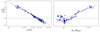 |
Fig. 4. Ratio of the observed radio fluxes to the results of Eq. (1) (using |


4. Functional dependency of the radio emission
In the JED-SAD paradigm, the evolution of the X-ray spectrum (hardness, energy cutoff, and flux) is described through the changes of two parameters, rJ and ṁin, controlling the balance between the power released through advection and radiation. In a similar way, we use both of these parameters to describe the radio flux.
We thus assume in this section a more general expression for the radio flux:
 (2)
(2)
This expression is similar to Eq. (1), but the indexes of the dependency on both ṁin and rJ are now free parameters. This new expression allows us to put all the dependency on rJ and ṁin in the parameters α and β,  acting then as a true constant in this respect. The term (rJ − risco)5/6 linked to the radial extension of the jet is re-expressed to isolate the dominant power dependency with rJ in α. We look for a unique triplet (
 , α, β) that could reproduce the whole radio data set.
4.1. Rising phase of the 2010 outburst
We first test Eq. (2) in the rising phase of outburst 4. We fit all 16 radio observations with simultaneous or quasi-simultaneous radio–X-ray data in XSPEC. We set rJ and ṁin of each observation to the best quasi-simultaneous X-ray fit values (obtained in Sect. 3). When simultaneously fitting X-ray and radio data, if the JED-SAD and reflections parameters are left free to vary simultaneously to  , α, and β, the X-ray fit is found to be significantly worse, especially around the iron line, for the benefit of a perfect match of the radio fluxes. By freezing the JED-SAD and reflections parameters to their best fit values obtained by fitting the X-rays, we instead chose to favor the X-ray fit for which we have a fully developed physically motivated spectral model. We implement in XSPEC a model to fit the radio emission following Eq. (2). We impose the same value of
  , α, and β for all the observations. The number of radio fluxes we use can be found in Table 1.
As the errors on the radio are sometimes quite small, we introduce a 10% systematic error on the radio fluxes to account for the non-simultaneity between the radio and X-ray observations and the few percent radio intrinsic variability (Corbel et al. 2000). This is done so that the fit is not driven by only one radio flux, but tries to reproduce all the fluxes within this 10% error margin. Furthermore, the maximum variation observed in the radio light curve is about 20% variation over three days (see Fig. A.1). Thus, within the one day delay between the radio and X-ray observations we do not expect variations exceeding the 10% systematic error we add, justifying the use of not exactly simultaneous X-ray and radio pointings. The effects of adding systematic errors is discussed in Appendix C.
The best fit gives  , α = −0.66 ± 0.32, and
  . The contours α–β are also reported as thin blue solid lines in Fig. 5. The fit reproduces all the radio fluxes within an error lower than 10% (see examples of residuals in Fig. 6) suggesting that Eq. (2) works adequately. The positive value of β is consistent with the observed correlation between the radio emission and the luminosity of the binary system. The negative value of α agrees with a decrease in the inner radius of the SAD when the system reaches bright hard states with stronger radio emission as expected in our JED-SAD approach (and similarly to most of the truncated disk models like Esin et al. 1997).
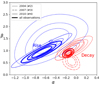 |
Fig. 5. Contour plots β–α for the rising (blue) and decaying (red) phases of the outburst of 2004 (outburst 2, dashed line), 2007 (outburst 3, dot-dashed line), and 2010 (outburst 4, thin solid line). The contours in thick solid lines represent the dependency when fitting all rising (blue) or decaying (red) phase radio fluxes simultaneously. Confidence contour levels correspond to 68%, 90%, and 99% (Δχ2 of 2.3, 4.61, and 9.2, respectively). The contours are obtained when fitting only the quasi-simultaneous radio–X-ray observations (not the interpolated radio observations). |
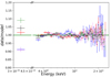 |
Fig. 6. Ratio of the data to the model for the best fit of 5 of the 16 multiwavelength observations (radio–X-ray) of the rising phase of the 2010 outburst (MJD 55217 in blue, 55259 in red, 55271 in black, 55288 in green, and 55292 in violet). Only five ratios are shown for purposes of visualization, but the best fit was obtained by using all the simultaneous or quasi-simultaneous radio–X-ray observation, fixing the JED-SAD parameters to the best fitting values obtained by fitting the X-ray spectra first, and then fitting the radio points with Eq. (2). |
In the second step we apply the same procedure to all the interpolated radio fluxes of the rising phase of outburst 4. Following the first step, we set rJ and ṁin to their best fit values obtained when fitting the X-ray alone. Then we reproduce the radio using the best fit values of  , α and β obtained previously to compute the expected radio flux FR using Eq. (2). The corresponding ratios Fobs/FR are reported in Fig. 7. There is almost no remaining dependency on rJ or ṁin. Compared to Fig. 4, this now shows a much more clustered distribution around 1, with a dispersion of about ±15%.
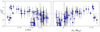 |
Fig. 7. Ratio of all radio fluxes of the rising phase of outburst 4 to the results of Eq. (2) as a function of rJ (left) and ṁin (right). The filled blue points represent the 16 quasi-simultaneous radio–X-ray observations, while the empty points represent the interpolated radio fluxes (see Appendix A). The radio observations are well reproduced using the values |
4.2. Decaying phase of the 2010 outburst
For the decaying phase of outburst 4 we proceeded similarly to the rising phase. We chose all eight observations, with simultaneous or quasi-simultaneous (differences less than 1 day) radio–X-ray observations of the decaying phase of outburst 4. We set the values of rJ and ṁin to the best X-ray fit, then we fit the radio fluxes using Eq. (2).
As a first test, we set  , α, and β to the best fit values obtained in the rising phase. The corresponding data/model ratio is plotted in Fig. 8. The top panel shows that using the value of
  of the rising phase in the decaying phase induces an error in the radio flux of up to a factor of 5. The bottom panel shows that even if we leave the scaling factor
  free, converging to the value 2.0 × 10⁻⁷, the radio flux is incorrect by a factor up to 1.8. Thus, the parameters
  , α, and β cannot have the same values as obtained in the rising phase.
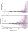 |
Fig. 8. Ratio of the data to the model for the best fit of five of the eight multiwavelength observations of the decaying phase of outburst 4 (MJD 55613 in blue, 55617 in red, 55620 in black, 55630 in green, and 55639 in violet). Top panel: all fits were done simultaneously, fixing the parameters of Eq. (2) to those found in the rising phase: |


Following what we present for the rising phase, we now leave  , α, and β free to vary, but linked between all the observations. The best fit values are
  ,
,  , and β = 1.02 ± 0.23. The corresponding confidence contour α–β is plotted as red thin solid lines in Fig. 5. It is clearly inconsistent with the blue contour obtained in the rising phase.
4.3. Comparison with the other outbursts
We constrain the functional dependency of the radio emission of the other outbursts by repeating a similar analysis. We thus need at least three observations taken in the corresponding rising and decaying phases to constrain the three free parameters α, β, and  . Only outburst 2 (in 2004) and the decaying phase of outburst 3 (in 2007) have the sufficient number of simultaneous or quasi-simultaneous radio and X-ray observations to apply our procedure. The number of radio fluxes we use for each phase of the outbursts can be found in Table 1. The corresponding contour plots of α–β are overplotted in Fig. 5 as dashed and dot-dashed lines, respectively. Two results are remarkable. First, and similarly to outburst 4, we need different functional dependencies of the radio emission with rJ and ṁin between the rising and decaying phase for outburst 2. Even more interestingly, the values obtained for α and β are in quite good agreement between the different outbursts, the contour of the decaying phase of outburst 3 also close to the contours of the decaying phases of outbursts 2 and 4. While this could be surprising given the simple expression used to model the radio emission, we believe that this result reveals intrinsic differences in the jet emission origin (see Sect. 5 for this discussion).
In the last step we use all the quasi-simultaneous radio observations, simultaneously fitting all the rising phase observations together with the same parameters α and β for all outbursts, but with different normalization  for each outburst. We did the same for all the decaying phase observations. The resulting α–β contours are plotted in Fig. 5 as thick solid lines.
The process confirms the two different and mutually inconsistent functional dependencies of the radio emission on rJ and ṁin between the rising and decaying phases observations. The radio flux observed in the rising phases is nicely reproduced (within about 15%) by the relation
 (3)
(3)
instead, in decaying phases it follows
 (4)
(4)
with a weaker dependency on rJ.
Some variations in  are required, however, to significantly improve the radio emission modeling. This can be seen in Fig. 9 where we report the ratio Fobs/FR using Eq. (3) to compute the radio flux if the observation is in the rising phase and Eq. (4) if in the decaying phase. In the top panel we use the same value
  for all outbursts. The ratios cluster around 1, although there is some scattering between the different phases of the different outbursts. We report in the bottom panel of Fig. 9 the same ratio but letting
  free to vary between outbursts and between the rising and decaying phases. The improvement is clear and almost all radio fluxes can be reproduced within a 20 % margin error. The different values of
  found are reported in Table 3. We observe variation up to a factor of three (e.g., between the rising phase of the 2002 and 2010 outbursts). This could be related to local changes in the radiative efficiency of the radio emission from outburst to outburst.
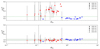 |
Fig. 9. Ratios of the observed radio fluxes to the modeled radio fluxes for all the quasi-simultaneous radio–X-ray observations of the four outbursts. Each outburst is represented using a different symbol (see legend). In blue are shown the rising phases and in red the decaying phases. The modeled radio fluxes were obtained using Eq. (2). The parameters are (α = −0.67, β = 0.94) for the rising phases and (α = −0.15, β = 0.9) for the decaying phases. Top panel: |


Values of  found for each phase of the outbursts.
5. Discussion
We present in this paper the first X-ray spectral fits of an X-ray binary using the JED-SAD model. Compared to previous works, we constructed model tables that enable the use of XSPEC for a direct fit procedure. We also constructed a reflection table, based on RELXILL, using as inputs the photon index and high-energy cutoff that best fit the JED-SAD spectral shapes. We obtained good fits for all the X-ray observations of GX-339-4 during the hard states observed by RXTE on the period 2002–2010 by only varying the accretion rate ṁin of our system and the transition radius rJ between the JED and the SAD.
As said in the Introduction, in the absence of a known physical law that would link these two parameters, we left them free to vary independently of each other in the fit procedure. This is the simplest approach to try to understand, and hopefully to physically interpret (see Ferreira et al., in prep.), their behavior.
Then radio emissions simultaneous to the X-rays (or quasi-simultaneous, with a one-day difference) were reproduced using a generic formula only depending on ṁin and rJ. One of the main results of this spectral analysis is the necessity of a different functional dependency of the radio emission on rJ and ṁin. The two different expressions for the radio emission are reported in Eqs. (3) and (4). We believe that this difference in functional dependency is a “back product” of the true physical link between rJ and ṁin.
5.1. Indications of different radiative behaviors between the rising and decaying phases
Observational clues on the jet behavior can be derived from a set of different diagnostics: (i) the radio spectral index αR, (ii) the measure of the spectral break frequency νbreak, (iii) timing properties, (iv) the correlation LR − LX, and (v) linking the radio luminosity LR to disk properties (ṁin,rJ). Items (i)–(iv) are discussed in this section, while item (v) is discussed in Sect. 5.2.
The radio spectral index αR can be analytically derived under the assumption of a self-absorbed synchrotron emission smoothly distributed along the jet. It depends on the particle distribution function, the jet geometry, and the way the dominant magnetic field varies with the distance (see Eq. (A.8) in the Appendix of Marcel et al. 2018b). There is no a priori reason to assume that these parameters should not vary in time. Observationally, however, there is no clear evidence of differences in the radio spectral index αR between the rising and decaying phases of GX 339-4 (Espinasse, priv. comm.; see also Koljonen & Russell 2019 for more detailed discussion on this point and Tremou et al. 2020 for the quiescent state case where the radio spectrum is clearly inverted). Although this is already an important piece of information, we note that these αR are derived within a rather limited radio band and might therefore not be fully representative of the whole jet spectrum (see, e.g., Péault et al. 2019).
The evolution of the spectral break frequency, νbreak, marking the transition from self-absorbed to optically thin jet synchrotron radiation, could however be different in the two phases (rising and decaying). The radio spectral index being flat or inverted in the hard state, the power of the jets is mainly sensitive to the position of the spectral break. Gandhi et al. (2011) measured this break at ∼5 × 10¹³ Hz in a bright hard state during the rise of the 2010–2011 outburst. By comparison, Corbel et al. (2013) constrain the break to be at lower frequency in the decaying phase, suggesting a less powerful jet in this phase. There is also a potential link between the X-ray hardness and the jet spectral break frequency, harder X-ray spectra having a higher νbreak (Russell et al. 2014; Koljonen et al. 2015). Interestingly, GX 339-4 shows on average a softer power law index in the decaying phase compared to the rising phase (see Fig. 10). Given the observed correlation between νbreak and the X-ray hardness, this also suggests a different behavior for νbreak (and consequently of the jet power) between the two phases.
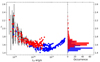 |
Fig. 10. Evolution of the hard X-ray power law index Γ during the four outbursts of GX339-4. Left: hard X-ray power law index Γ as a function of the 3–9 keV X-ray luminosity of the pure hard state observations during the four GX339-4 outbursts (data from Clavel et al. 2016). In blue the rising phase and in red the decaying phase. Right: histograms of Γ. These distributions are subject to a certain number of observational biases: inclusion of error bars and the number of observations per phase. |
There are other indications that the accretion (through X-ray emission) and ejection (through radio emission) processes could behave differently at the beginning and the end of the outburst. At first sight the radio–X-ray correlation followed by GX339-4 agrees with a linear correlation of index ∼0.7 in log-log space (e.g., Corbel et al. 2000, 2003, 2013) even down to very quiescent states (Tremou et al. 2020), but a more careful analysis shows the presence of wiggles along this linear correlation, especially between the high- and low-luminosity states (e.g., Corbel et al. 2013, Fig. 8). When looking more precisely at the rising and decaying phase, two different correlations may even be observed (Islam & Zdziarski 2018).
These differences may be linked to a change in the radiative efficiency of the X-ray corona with luminosity. The low X-ray luminosity states, below 2–20% of the Eddington luminosity, are potentially less radiatively-efficient than the high X-ray luminosity states (Koljonen & Russell 2019; Marcel et al., in prep.). As noticed by Koljonen & Russell (2019), these changes of the accretion flow properties could affect the jet launching, and therefore its radio emission properties.
In the JED-SAD model, the accretion power available in the accretion flow, ![Mathematical equation: $ \displaystyle P_{\mathrm{acc}}=\frac{GM\dot{M}}{2R_{\mathrm{isco}}}\left [1-\left (\frac{r_{\mathrm{isco}}}{r_J}\right )^{1-p}\right ] $](/articles/aa/full_html/2022/01/aa41182-21/aa41182-21-eq64.gif) (see Sect. 1 for the definition of p and b), is released in three different forms: advection, radiation, and ejection. The first two occur inside the JED, and their sum is defined as PJED = (1 − b) Pacc. The ejection power is released in the jets and is defined as Pjets = b Pacc. We also define the ratio ηR = LR/Pjets and the ratio ηX = L3 − 9 keV/PJED that can be respectively interpreted as the radiative efficiency in the radio and X-ray bands. We report in Fig. 11 the ratio ηR7 as a function of the ratio ηX for the rising phase (blue points) and the decaying phase (red points) of the outbursts. We highlight in Fig. 11 the observations (labeled a to e) presented in Fig. 2 to mark the chronological evolution along an outburst. Figure 11 mostly depends on the well-constrained mass accretion rate obtained with our fits of each X-ray observations.
(see Sect. 1 for the definition of p and b), is released in three different forms: advection, radiation, and ejection. The first two occur inside the JED, and their sum is defined as PJED = (1 − b) Pacc. The ejection power is released in the jets and is defined as Pjets = b Pacc. We also define the ratio ηR = LR/Pjets and the ratio ηX = L3 − 9 keV/PJED that can be respectively interpreted as the radiative efficiency in the radio and X-ray bands. We report in Fig. 11 the ratio ηR7 as a function of the ratio ηX for the rising phase (blue points) and the decaying phase (red points) of the outbursts. We highlight in Fig. 11 the observations (labeled a to e) presented in Fig. 2 to mark the chronological evolution along an outburst. Figure 11 mostly depends on the well-constrained mass accretion rate obtained with our fits of each X-ray observations.
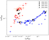 |
Fig. 11. Radio emission efficiency (LR = L9 GHz/PJets) vs. X-ray emission efficiency (LX = L3 − 9 keV/PJED) during the outbursts of GX339-4. The blue points are the rising phases. The red points are the decaying phases. The symbols distinguish the different outbursts: diamonds for 2002, squares for 2004, dots for 2007, and triangles for 2010 (filled for the quasi-simultaneous observations and empty for the interpolated radio fluxes). We highlighted the five observations (labeled a to e) presented in Fig. 2 to provide the chronological evolution of an outburst. |
The blue points of the rising phases follow a similar trend for all the outbursts with a change in the X-ray and radio radiative efficiency by a factor of ∼4 and ∼2, respectively. In the decaying phase, however, each outburst clusters at the same radio and X-ray radiative efficiency. Interestingly, the radio radiative efficiency changes from outburst to outburst, while the X-ray radiative efficiency stays roughly constant at ηX ∼ 3 − 4 × 10⁻², the lowest values observed in the rising phase. These results indeed suggest a change in the radiative properties of the accretion-ejection structure between the beginning and the end of the outburst, and it is possible that it has some impact on the functional dependency of the radio emission highlighted in this paper. Contrary to the conclusion of Koljonen & Russell (2019), however, the accretion rate does not seem to be the only parameter that controls the evolution of ηR. Looking at outburst 2 and 4 separately, ηR stays roughly constant in the decaying phase of each outburst, whereas ṁin varies by at least a factor of 10 (see Fig. 3). In addition, different radio efficiencies are observed between each outburst during the decaying phases even at similar values of ṁin. Something else also seems to be at work.
5.2. Possible changes in the dynamical ejection properties
The existence of two functional dependencies FR(ṁin,rJ) raises a profound question. Radiative processes in jets are local and are independent of disk parameters such as ṁin and rJ. However, the time evolution FR(t) can be quite accurately reproduced with a function of (ṁin,rJ), which shows that global jet parameters do actually depend on them. These parameters, which constitute the jet dynamics, are for instance the magnetic field strength and geometry, the jet collimation degree, the existence of internal shocks or even jet instabilities. Our findings seem therefore to highlight two different jet dynamics.
5.2.1. A possible threshold in ṁin
The hard state data sets of the rising and decaying phases used in this analysis do not overlap in terms of accretion rate. Only two out of the 28 radio observations of the rising phases require a mass accretion rate comparable to those observed during the decaying phases. All the others have a higher mass accretion rate than the decaying phases. This is an observational bias due to the difficulties in catching the source as quickly as possible at the beginning of the outburst. However, the detected difference in the functional dependency of FR could be due to some threshold in ṁin that could, in turn, translate into some difference in the way the radio emission scales with the disk parameters. Above the threshold the radio emission would follow Eq. (3), and below the threshold Eq. (4). Given the insufficient number of low accretion rate hard states in the rising phases, our analysis cannot test this possibility. Clearly, more observations are needed to assess this hypothesis.
We do not favor this interpretation, however. The main reason is that the rising and decaying hard states are temporally disconnected. The source stays in the soft state between these two hard-state phases for several months, and thus do not share the same history. The hard states in the rising phase come from a quiescent, already radio emitting state, while the hard states in the decaying phase come from soft radio silent states. This supports a link with the global jet structure (as proposed in Sect. 5.2.2) rather than a threshold in ṁin.
5.2.2. A change in the dominating ejection process
Since the commonly invoked radiative process is synchrotron, the first thing that comes to mind to explain this difference is the magnetic field strength. The only reasonable assumption to make is that this field is proportional to the field anchored at the JED, which writes (see Marcel et al. 2018b for more details)
 (5)
(5)
where μ is the magnetization, ms the accretion Mach number, P* = min*c2, and  . Assuming constant JED parameters μ = 0.5 and ms = 1.5 used in our model, we evaluate the magnetic field strength measured in risco at around 108 G during the outbursts.
It should be noted that a JED exists within a small interval [μmin, μmax] of disk magnetization μ, with μmin ∼ 0.1 and μmax ∼ 0.8 (Ferreira 1997). The existence of such an interval has led Petrucci et al. (2008) to propose that the hysteresis observed in XrBs could be a consequence of a JED switch-off with μ = μmin and switch-on at μ = μmax. In the spectral analysis shown in the present paper, we suppose a constant μ since, as shown in Marcel et al. (2018b), the JED spectra are poorly affected by μ within the allowed parameter space. However, the possible difference in magnetization between the rising and decaying phase could also have a direct impact on the jet dynamical and radiative properties, explaining the change of the observed radio behavior. According to Eq. (5), a dichotomy of the magnetization μ at a given value of the mass accretion rate ṁin entails a dichotomy in the magnetic field strength. Thus, the rising phase, switching-off with μ = μmin, would present a weaker magnetic field strength compared to the decaying phase, switching-on with μ = μmax. This difference in the magnetic field strength could play a role in the difference of functional dependency of the radio emission. This could also explain the higher radio efficiencies observed in Fig. 11 during the decaying phases (e.g., Casella & Pe’er 2009).
Another possibility could be suggested by the most recent numerical simulations showing that the vertical magnetic field is carried in and accumulates around the black hole (building up a magnetic flux Φbh) until the surrounding disk magnetization reaches a maximum value near unity (see, e.g., Tchekhovskoy et al. 2011; Liska et al. 2020). In our view, the inner disk regions are nothing else than a JED driving a Blandford & Payne (BP, Blandford & Payne 1982) jet, although a Blandford & Znajek (BZ, Blandford & Znajek 1977) spine launched at its midst has attracted more attention in the literature8. Then another possible explanation for the existence of two functional dependencies for FR(ṁin,rJ) could be that jets are two-component MHD outflows: a BZ spine, tapping into the rotational energy of the black hole, surrounded by a BP jet, tapping into the accretion energy reservoir of the disk. The jet dynamics and subsequent radio emission then depend on the relative importance of these two flows, which can be roughly measured by the ratio of the magnetic flux associated with each component, namely Φbh for the spine and ΦJED for the outer BP jet. By construction, Φbh builds upon ΦJED and reaches large values, such as  , only if a large magnetic flux is available initially in the disk (Tchekhovskoy et al. 2011; Liska et al. 2020). The functional dependency on rJ that we observe for the radio flux in our fits of the rising phase spectra could thus come from the dependency of
  on rJ.
A simple scenario can then be designed and is sketched in Fig. 12. During the rising hard-state phase, rJ is initially large and decreases in time (top right). The system comes from a quiescent state and the presence of a JED over a large radial extent allowed the disk to build up a maximum Φbh. The spine is very important and affects the overall jet dynamics, which translates into a radio flux described by Eq. (3). When the disk magnetization becomes too small, the JED transits to a SAD accretion mode (left, top and bottom). The magnetic field diffuses away, thereby decreasing Φbh, and no more jets are observed (neither BP nor BZ). As long as the system remains in the soft state, the field keeps on diffusing away until some equilibrium is eventually reached. At some point however the outburst declines, which translates into a decrease in the inner disk pressure, and thus an increase in the disk magnetization. In this decaying phase an inner JED becomes re-ignited inside-out, with its bipolar BP jets, but with a limited magnetic flux available (bottom right). By construction, Φbh remains small and the BZ spine has a limited impact on the overall jet dynamics. This would translate into a radio flux described by Eq. (4) until the JED is rebuilt over a large enough radial extent.
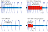 |
Fig. 12. Sketches of the inner regions of an accretion flow around a black hole during the different phases of the outburst. Top right: in the rising hard phase the JED is settled over a large region (RJ is large), leading to efficient magnetic flux accumulation on the black hole. The radio emission arises from a two-component outflow, made of an important BZ spine surrounded by a BP jet. Top left to bottom left: during the soft state there is no more JED, the magnetic field diffuses away, and the BP and BZ jets both disappear. Little or no weak radio emission is expected (jetline). Bottom right: in the decaying phase a JED reappears in the innermost region, and the magnetic field advection becomes efficient again. The magnetic flux on the black hole is still weak, and the BZ spine has little or no impact on the jet dynamics and subsequent radio emission. |
There are many uncertainties in our different interpretations, since our JED-SAD modeling has its own simplifications. This last scenario is only an attempt to provide an explanation to our puzzling finding. Quite interestingly, it also provides a means of observationally testing it. It relies on the existence of a BZ spine in the case of GX 339-4, which is a black hole candidate. Around a neutron star the invoked scenario of magnetic flux accumulation into the central object clearly should not work. It would therefore be useful to investigate any changes in the radio properties during the rise and decay phases for neutron star binaries.
This scenario may look similar to the ones proposed by Begelman & Armitage (2014) or Kylafis & Belloni (2015) where the presence of a hot inner corona (an ADAF-like accretion flow in both cases) would help in accumulating or creating the required magnetic field that will eventually produce a jet. However, in these two approaches it is not clear why the process would differ between the rising and decaying phases, and how the functional dependency of the radio emission would depend on the ADAF properties. Clearly, more dedicated work should be done in this respect.
5.3. Effects of the JED-SAD parameters
In the results shown in this work we use the same values of the JED-SAD parameters b, ms, and p as used in M19 and M20. A detailed study of the JED-SAD parameter space has already been performed (see Marcel et al. 2018b Sect. 4) and converges on these values in the case of GX 339-4. The parameter p has almost no spectral impact in the RXTE/PCA energy range (3–25 keV); this can be seen in Fig. 10 of Marcel et al. (2018b) (p was called ξ at the time). Thus, we do not expect any variation in the fits. Letting p remain free would result in an unconstrained parameter. The main impact of the parameters b and ms is a variation of the maximum temperature in the JED, and results in a variation of the high-energy cutoff of the hard X-ray emission. However, the high-energy cutoff is not visible within the RXTE/PCA energy range used in our fitting procedure. We are then unable to constrain these parameters from the data and choose to set them to the same values used by M19 and M20. This also allows us to compare the evolution of the main JED-SAD parameters rJ and ṁin with the qualitative results obtained by M19 and M20.
However, we study the impact of using other values of ms or b. The global trend of the parameters is similar, with only slightly different values of rJ and ṁin (see Figs. D.1 and D.2 in the Appendix). The biggest changes are observed with the different values of ms. We thus concentrate on this parameter to see the effect of its value on the α − β contours (see Fig. D.3). The contour plots of the rising and decaying phase vary for different values of ms; however, they are never consistent between each other, leaving our main conclusions unchanged: we need two different functional dependencies between the rising and decaying phases.
6. Conclusion
We presented in this paper the first direct fit of the X-ray data of an X-ray binary with our JED-SAD model. We constructed fits format tables that can be used in XSPEC. This includes a reflection table based on the XILLVER reflection model (Garcia et al. 2013). We applied our model to the X-ray observations of GX339-4, focusing on the “pure” hard-state phases of the four outbursts observed during the RXTE lifetime. We deduced from the fits the temporal evolution of the main parameters of the JED-SAD configurations: the inner accretion rate ṁin and the transition radius rJ between the inner JED and the outer SAD (see Fig. 3). This evolution is in relatively good agreement with the qualitative estimates done by M19 and M20; however, our spectral fit procedure puts much stronger constraints on rJ.
We were also able to put constraints on the functional dependency of the radio emission with rJ and ṁin for all outbursts of GX 339-4. Assuming a general radio flux expression  , we were able to constrain the values of α and β for the different outbursts. These values appear consistent between the different rising phases or the different decaying phases. However, the rising or high mass accretion rate and decaying or low accretion rate phases solutions differ significantly. In the rising phase the radio emission varies as
  , while in the decaying phase the radio emission has a weaker dependency with rJ and varies as
  . While the exact values of the indexes depend slightly on the JED-SAD parameters, the two solutions obtained for the rising and the decaying phases are always mutually exclusive. A significant improvement in the fit of the radio fluxes is obtained by letting the scaling factor
  free to vary between the different phases. The observed variation (up to a factor 2) could correspond to a change in the radiative efficiency of the radio emitting process from outburst to outburst.
We suggest a few explanations for the difference in the functional dependency of the radio emission with rJ and ṁin between the rise and decay phases. A clear understanding is challenging given the scarce information we have on crucial jet parameters like the magnetic field strength and geometry, the jet collimation degree, the existence of internal shocks, or even jet instabilities. A possible scenario relies on a change of the relative importance of the Blandford & Znajeck versus Blandford & Payne processes in the radio emitting process due to the expected evolution of the magnetic field strength in the inner part of the accretion flow.
All results of this paper should be tested on other XrBs and on more recent outbursts of GX339-4. It would be also interesting to see how the case of neutron stars (where no BZ is expected) or objects belonging to the so-called outlier population (Coriat et al. 2011) would compare with our present results. Especially since the outliers present a steep power index in the radio–X-ray plane at high luminosity, similar to that observed in neutron star binaries. This will be the focus of a forthcoming paper.
However a better result was obtained when using a constant, but different,  for the rising and decaying phase with
  (G. Marcel, priv. comm.).
“Failed” outbursts only present hard states and no transition to the soft states before going back to quiescence.
Before 2009 the radio band was 128 MHz wide and centered at 8.64 GHz. After 2009 it was 2 GHz wide and centered at 9 GHz.
In the previous papers (Marcel et al. 2018a,b, 2019), this parameter was called ξ. However, to avoid confusion with the ionization parameter of the reflection component, here we introduce the notation p.
Such a high iron abundance could be a consequence of the XILLVER reflection model used. A new version of this model, with higher disk density, gives a value closer to solar values (e.g., Tomsick et al. 2018; Jiang et al. 2019).
Even though the high-energy cutoff is not visible in the energy range we fit, the JED-SAD parameters we obtain predict a decrease in the high-energy cutoff during the rising phase, similarly to what is observed (Motta et al. 2009; Droulans et al. 2010).
In the case of the 2010 outburst, the full triangles are quasi-simultaneous radio fluxes, whereas the empty triangles use the interpolated radio luminosity LR computed for all the X-ray observations (see Fig. A.1).
The inner disk regions are usually called magnetically arrested accretion disks (MADs) (Narayan et al. 2003; Tchekhovskoy et al. 2011); however, as accurately noted by McKinney et al. (2012), a thin or even slim disk is not arrested. The deviation from Keplerian rotation is only on the order of the disk thickness, and its structure resembles the JED, with a near-equipartition magnetic field.
Acknowledgments
The authors acknowledge funding support from CNES and the French PNHE.
References
- Arnaud, K. A. 1996, in Astronomical Data Analysis Software and Systems V, eds. G. H. Jacoby, & J. Barnes, ASP Conf. Ser., 101, 17 [NASA ADS] [Google Scholar]
- Begelman, M. C., & Armitage, P. J. 2014, ApJ, 782, L18 [NASA ADS] [CrossRef] [Google Scholar]
- Bel, M. C., Rodriguez, J., D’Avanzo, P., et al. 2011, A&A, 534, A119 [NASA ADS] [CrossRef] [EDP Sciences] [Google Scholar]
- Blandford, R. D., & Znajek, R. L. 1977, MNRAS, 179, 433 [NASA ADS] [CrossRef] [Google Scholar]
- Blandford, R., & Payne, D. 1982, MNRAS, 199, 883 [CrossRef] [Google Scholar]
- Casella, P., & Pe’er, A. 2009, ApJ, 703, L63 [Google Scholar]
- Clavel, M., Rodriguez, J., Corbel, S., & Coriat, M. 2016, Astron. Nachr., 337, 435 [Google Scholar]
- Corbel, S., Fender, R. P., Tzioumis, A. K., et al. 2000, A&A, 359, 251 [NASA ADS] [Google Scholar]
- Corbel, S., Nowak, M. A., Fender, R. P., Tzioumis, A. K., & Markoff, S. 2003, A&A, 400, 1007 [NASA ADS] [CrossRef] [EDP Sciences] [Google Scholar]
- Corbel, S., Fender, R., Tomsick, J., Tzioumis, A., & Tingay, S. 2004, ApJ, 617, 1272 [CrossRef] [Google Scholar]
- Corbel, S., Coriat, M., Brocksopp, C., et al. 2013, MNRAS, 428, 2500 [Google Scholar]
- Coriat, M., Corbel, S., Prat, L., et al. 2011, MNRAS, 414, 677 [Google Scholar]
- De Marco, B., Ponti, G., Petrucci, P.-O., et al. 2017, MNRAS, 471, 1475 [NASA ADS] [CrossRef] [Google Scholar]
- Done, C., Gierlinski, M., & Kubota, A. 2007, A&ARv, 15, 1 [Google Scholar]
- Droulans, R., Belmont, R., Malzac, J., & Jourdain, E. 2010, ApJ, 717, 1022 [NASA ADS] [CrossRef] [Google Scholar]
- Dunn, R. J. H., Fender, R. P., Körding, E. G., Belloni, T., & Cabanac, C. 2010, MNRAS, 403, 61 [Google Scholar]
- Esin, A. A., McClintock, J. E., & Narayan, R. 1997, ApJ, 489, 865 [NASA ADS] [CrossRef] [Google Scholar]
- Fabian, A. C., Lohfink, A., Belmont, R., Malzac, J., & Coppi, P. 2017, MNRAS, 467, 2566 [Google Scholar]
- Fender, R., & Belloni, T. 2004, Annu. Rev. Astron. Astrophys., 42, 317 [Google Scholar]
- Ferreira, J. 1997, A&A, 319, 340 [Google Scholar]
- Ferreira, J., & Pelletier, G. 1995, A&A, 295, 807 [NASA ADS] [Google Scholar]
- Ferreira, J., Petrucci, P.-O., Henri, G., Saugé, L., & Pelletier, G. 2006, A&A, 447, 813 [NASA ADS] [CrossRef] [EDP Sciences] [Google Scholar]
- Frank, J., King, A., & Raine, D. J. 2002, Accretion Power in Astrophysics, (Cambridge University Press) [Google Scholar]
- Fürst, F., Nowak, M., Tomsick, J., et al. 2015, ApJ, 808, 122 [CrossRef] [Google Scholar]
- Gallo, E., Fender, R. P., & Pooley, G. 2003, MNRAS, 344, 60 [NASA ADS] [CrossRef] [Google Scholar]
- Gallo, E., Miller, B. P., & Fender, R. 2012, MNRAS, 423, 590 [Google Scholar]
- Gandhi, P., Blain, A., Russell, D., et al. 2011, ApJ, 740, L13 [NASA ADS] [CrossRef] [Google Scholar]
- Garcia, J., Dauser, T., Reynolds, C., et al. 2013, ApJ, 768, 146 [NASA ADS] [CrossRef] [Google Scholar]
- García, J. A., Steiner, J. F., McClintock, J. E., et al. 2015, ApJ, 813, 84 [Google Scholar]
- Haardt, F., Maraschi, L., & Ghisellini, G. 1997, ApJ, 476, 620 [CrossRef] [Google Scholar]
- Hameury, J.-M., Menou, K., Dubus, G., Lasota, J.-P., & Hure, J.-M. 1998, MNRAS, 298, 1048 [Google Scholar]
- Heinz, S., & Sunyaev, R. A. 2003, MNRAS, 343, L59 [Google Scholar]
- Islam, N., & Zdziarski, A. A. 2018, MNRAS, 481, 4513 [Google Scholar]
- Jacquemin-Ide, J., Ferreira, J., & Lesur, G. 2019, MNRAS, 490, 3112 [Google Scholar]
- Jacquemin-Ide, J., Lesur, G., & Ferreira, J. 2021, A&A, 647, A192 [EDP Sciences] [Google Scholar]
- Jiang, J., Fabian, A. C., Wang, J., et al. 2019, MNRAS, 484, 1972 [NASA ADS] [CrossRef] [Google Scholar]
- Koljonen, K. I. I., & Russell, D. M. 2019, ApJ, 871, 26 [Google Scholar]
- Koljonen, K., Russell, D., Fernández-Ontiveros, J., et al. 2015, ApJ, 814, 139 [CrossRef] [Google Scholar]
- Kylafis, N. D., & Belloni, T. M. 2015, A&A, 574, A133 [NASA ADS] [CrossRef] [EDP Sciences] [Google Scholar]
- Laor, A. 1991, ApJ, 376, 90 [Google Scholar]
- Liska, M., Tchekhovskoy, A., & Quataert, E. 2020, MNRAS, 494, 3656 [Google Scholar]
- Marcel, G., Ferreira, J., Petrucci, P.-O., et al. 2018a, A&A, 617, A46 [NASA ADS] [CrossRef] [EDP Sciences] [Google Scholar]
- Marcel, G., Ferreira, J., Petrucci, P.-O., et al. 2018b, A&A, 615, A57 [NASA ADS] [CrossRef] [EDP Sciences] [Google Scholar]
- Marcel, G., Ferreira, J., Clavel, M., et al. 2019, A&A, 626, A115 [NASA ADS] [CrossRef] [EDP Sciences] [Google Scholar]
- Marcel, G., Cangemi, F., Rodriguez, J., et al. 2020, A&A, in press [Google Scholar]
- Martocchia, A., & Matt, G. 1996, MNRAS, 282, L53 [NASA ADS] [CrossRef] [Google Scholar]
- Matt, G., Perola, G., & Piro, L. 1991, A&A, 247, 25 [Google Scholar]
- McKinney, J. C., Tchekhovskoy, A., & Blandford, R. D. 2012, MNRAS, 423, 3083 [Google Scholar]
- Merloni, A., & Fabian, A. C. 2001, MNRAS, 321, 549 [NASA ADS] [CrossRef] [Google Scholar]
- Miller, J., Reynolds, C., Fabian, A., et al. 2008, ApJ, 679, L113 [CrossRef] [Google Scholar]
- Miniutti, G., & Fabian, A. 2004, MNRAS, 349, 1435 [NASA ADS] [CrossRef] [Google Scholar]
- Motta, S., Belloni, T., & Homan, J. 2009, MNRAS, 400, 1603 [CrossRef] [Google Scholar]
- Narayan, R., Igumenshchev, I. V., & Abramowicz, M. A. 2003, PASJ, 55, L69 [NASA ADS] [Google Scholar]
- Parker, M., Tomsick, J., Kennea, J., et al. 2016, ApJ, 821, L6 [NASA ADS] [CrossRef] [Google Scholar]
- Péault, M., Malzac, J., Coriat, M., et al. 2019, MNRAS, 482, 2447 [CrossRef] [Google Scholar]
- Petrucci, P.-O., Ferreira, J., Henri, G., & Pelletier, G. 2008, MNRAS, 385, L88 [NASA ADS] [CrossRef] [Google Scholar]
- Petrucci, P. O., Ferreira, J., Henri, G., Malzac, J., & Foellmi, C. 2010, A&A, 477 [Google Scholar]
- Remillard, R. A., & McClintock, J. E. 2006, ARA&A, 44, 49 [Google Scholar]
- Russell, T. D., Soria, R., Miller-Jones, J. C., et al. 2014, MNRAS, 439, 1390 [NASA ADS] [CrossRef] [Google Scholar]
- Scepi, N., Lesur, G., Dubus, G., & Jacquemin-Ide, J. 2020, A&A, 641, A133 [EDP Sciences] [Google Scholar]
- Shakura, N. I., & Sunyaev, R. A. 1973, A&A, 24, 337 [NASA ADS] [Google Scholar]
- Tchekhovskoy, A., Narayan, R., & McKinney, J. C. 2011, MNRAS, 418, L79 [NASA ADS] [CrossRef] [Google Scholar]
- Tomsick, J. A., Parker, M. L., García, J. A., et al. 2018, ApJ, 855, 3 [NASA ADS] [CrossRef] [Google Scholar]
- Tremou, E., Corbel, S., Fender, R. P., et al. 2020, MNRAS, 493, L132 [NASA ADS] [CrossRef] [Google Scholar]
- Wang-Ji, J., García, J. A., Steiner, J. F., et al. 2018, ApJ, 855, 61 [NASA ADS] [CrossRef] [Google Scholar]
- Zanni, C., Ferrari, A., Rosner, R., Bodo, G., & Massaglia, S. 2007, A&A, 469, 811 [NASA ADS] [CrossRef] [EDP Sciences] [Google Scholar]
- Zdziarski, A. A., Gierlinski, M., Mikolajewska, J., et al. 2004, MNRAS, 351, 791 [NASA ADS] [CrossRef] [Google Scholar]
- Zdziarski, A. A., Ziółkowski, J., & Mikołajewska, J. 2019, MNRAS, 488, 1026 [Google Scholar]
Appendix A: Outburst 4 radio interpolation
With 80 almost daily X-ray observations and 24 radio flux measurements, the radio–X-ray survey of the hard states of the 2010 outburst of GX339-4 is the best in the available archive of RXTE. Considering the steady jet expected during the hard states of an outburst and the evenly spread radio survey, we opted to linearly interpolate the radio light curve to obtain a radio flux for each X-ray observation. In Fig. A.1 we plot the radio light curve.
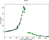 |
Fig. A.1. Radio light curve of outburst 4 during its hard states: between MJD 55208 and 55293, and between MJD 55608 and 55646. The green squares are the observed radio data. The blue dashed line is the linearly interpolated function. The black diamonds are the interpolated radio fluxes at the date of the X-ray observations. |
Appendix B: Fitting the decaying phase of outburst 4
In Fig. B.1 we plot the evolutions of rJ and ṁin during outburst 4. The blue dashed line represents the final results presented in Fig. 3 used for the study. The red dashed line represents the initial results obtained by our fitting procedure. In this appendix we explain why we rejected the results of this fitting procedure, and how we obtained the final results for the decaying phase of outburst 4 using a maximum likelihood method.
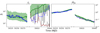 |
Fig. B.1. Results of the fitting procedure for outburst 4. On the left side is shown the transition radius rJ between the JED and the SAD, on the right side the mass accretion rate ṁin. Each side is divided horizontally between the rising and decaying phase of each outburst. The green solid line represents the results from M19 and M20, and the green region where their minimization function varies by less than 10% with respect to its minimum. The blue dashed line shows the results presented in Fig. 3 and the black vertical bar the associated 90% confidence range. The red dashed line represents the initial fitting results for the decaying phase of outburst 4. |
The main disagreement of the fitting procedure with M19 was observed in the decaying phase of outburst 4. The fits yielded quite small values of rJ (∼5RG) and a decrease in the transition radius with time (Fig. B.1, red), which is not expected in the JED-SAD paradigm and in contradiction with the evolution observed by M19, although their constraints are quite large. We report in Fig B.2 the evolution of the χ2 statistic along the parameter space of rJ for a few observations of this decaying phase. These observations show a non-trivial χ2 space with multiple local minimums. Most of them presented either a better fit or a statistically equivalent fitting solution at higher rJ. For some reason, Xspec did not find these solutions even during the error calculations. In Fig. B.3 we represent Markov chain Monte Carlo (MCMC) tests for one of these observations (MJD 55630), starting from the higher (red) and lower (black) rJ solutions. In both cases, the procedure converged to a reasonable solution within a few steps (< 5). When starting with the lower rJ solution, the procedure first explores only the lower rJ values. It is only after ∼ 2500 steps that it explores the higher rJ solutions, and in the last 1000 steps, both procedures only explore the higher rJ solution. These higher rJ solutions were further motivated by the fact that high values of rJ naturally appear in outbursts 2 and 3 (see Fig. 3). For these different reasons, we set rJ to this solution for each observation of the decaying phase of outburst 4.
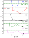 |
Fig. B.2. Evolution of the |
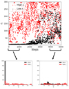 |
Fig. B.3. MCMC procedure for observation 55630 (see the χ2 parameter space in Fig. B.2 in green) starting from two different initial priors. In black starting with a lower rJ prior, in red starting with a higher rJ prior. Bottom: histograms of rJ during the first 1000 steps (left) and the last 1000 steps (right). Both procedures explore only the higher rJ solution. |
A similar process could have been applied to the decaying phase of the other outbursts; however, the lack of radio flux where similar problems were encountered made this issue non-critical for the rest of the study.
Appendix C: Effects of the systematic error
In this section we show the effects of adding systematic errors to our radio fluxes. The reasoning behind this addition is that we accept a 10% error on the reproduction of the radio fluxes. As the χ2 statistic gives more weight to the observations with small errors, without systematic errors added the fit is mostly driven by a few fluxes and does not match our quality criterion. Our goal is to reproduce all the radio fluxes within a 10-20% error margin. Adding a systematic error to all fluxes increases the relative weight of the observations with higher uncertainty compared to the ones with low flux error.
However this has a major impact on the size of the confidence contour β-α that we obtain. These contours depend directly on the χ2 plane of our parameter space. In Fig. C.1 we plot the confidence contour for a 90% confidence level (Δχ2 = 4.61) for all the rising phase observations (in blue) and for all the decaying phase observations (in red), and for different values of systematic errors added to the radio fluxes (0%, 5%, and 10% depending on the thickness of the line). As expected, the larger the systematic error added, the larger the contour plot, but even with a 10% systematic error the rising phase solution and decaying phase solution are inconsistent.
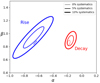 |
Fig. C.1. 90% Confidence contours β–α for different values of systematic error added to the radio fluxes (0%, 5%, and 10%). The thicker the line, the larger the systematic error added. Shown are the contours for all the rising phase observations (in blue) and the contours for all the decaying phase observations (in red). |
Appendix D: Impact of the other JED-SAD parameters
In this study we set the values of the parameters ms, p, and b to that used by M19. Marcel et al. (2018a) already performed a study of the parameter space and converged on these values. However, as the main spectral impact of ms and b is a variation of the high-energy cutoff, which is not visible inside the RXTE/PCA energy range, we are faced with unconstrained parameters. In this paragraph we present the same study reproduced using other set values of ms and b. In Figs. D.1 and D.2, we plot the fitting results obtained for different values of ms and b. The global trend of the parameters is similar; however, the values of rJ and ṁin are slightly different. The biggest difference is observed with the different values of ms. In Fig. D.3 we plot the corresponding contour regions α-β for the different values of ms. For the decaying phase observations, we used the procedure described in Appendix B to obtain the transition radius rJ for eight quasi-simultaneous observations used for the contour plots. The contours obtained for different values of ms are not always consistent with each other. However, in each case the rising phase and decaying phase contours are inconsistent. This implies that we always have two different behaviors for the radio between the rising and decaying phase regardless of the values of ms and b that we use in the fits.
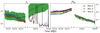 |
Fig. D.1. Results of the fitting procedure for outburst 4. On the left side is shown the transition radius rJ between the JED and the SAD, on the right side the mass accretion rate ṁin. Each side is divided horizontally between the rising and decaying phase of each outburst. The green solid line represents the results from M19, and the green region where the minimization function varies by less than 10% with respect to its minimum. The blue, orange, and purple dashed lines show the results of the automatic fitting procedure using different values of ms (1.0, 1.5, and 2.0, respectively). |
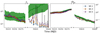 |
Fig. D.2. Results of the fitting procedure for outburst 4. On the left side is shown the transition radius rJ between the JED and the SAD, on the right side the mass accretion rate ṁin. Each side is divided horizontally between the rising and decaying phase of each outburst. The green solid line represents the results from M19 and M20, and the green region where the minimization function varies by less than 10% with respect to its minimum. The blue, orange, and purple dashed lines show the results of the automatic fitting procedure using different values of b (0.1, 0.3, and 0.5, respectively). |
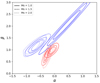 |
Fig. D.3. Confidence contours β-α for different values of ms used in the fitting procedure of outburst 4: 1.0 (solid line), 1.5 (dashed line), and 2.0 (dotted line). In all cases the rising phase contour and decaying phase contour are inconsistent. |
All Tables
All Figures
|
Fig. 1. GX 339-4 X-ray light curve in the 3–200 keV energy band of the 2000–2010 decade obtained with the Clavel et al. (2016) fits. The violet filled region shows the power law unabsorbed flux, while the cyan region represents the disk unabsorbed flux. The selected spectra for this study are highlighted in gray: the rising and decaying hard states of the four outbursts (1, 2, 3, and 4). At the top the red lines represent the date when steady radio fluxes were observed at 9 GHz (from Corbel et al. 2013). |
| In the text | |
|
Fig. 2. Best fits of some observations of outburst 4. Top left: hardness intensity diagram of outburst 4. The blue diamond shows the hard state used for this outburst. The five red points are the five observations plotted in the different figures from a to e. a–e: best fit spectra and the data/model ratio for the five observations indicated in red in the HID. The gray region shows the PCA energy range used for the fit. The data are in black and the best fit model in gray; the JED spectrum is in red, the SAD spectrum in green, and the reflection component in blue. The best fit parameters for each observation are listed in Table 2. |
| In the text | |
|
Fig. 3. Results of the fitting procedure. Left: transition radius rJ (from risco to 300) between the JED and the SAD. Right: mass accretion rate ṁin. Each side is divided vertically between the four outbursts and horizontally between the rising and decaying phase of each outburst. The green solid line represent the results from M19 and M20, and the green region indicates where the minimization function varies by less than 10% with respect to its minimum. The blue dashed line shows the results of the fitting procedure and the black vertical bar the associated 90% confidence range. The decaying phase of outburst 4 is the subject of Appendix B. |
| In the text | |
|
Fig. 4. Ratio of the observed radio fluxes to the results of Eq. (1) (using |
| In the text | |
|
Fig. 5. Contour plots β–α for the rising (blue) and decaying (red) phases of the outburst of 2004 (outburst 2, dashed line), 2007 (outburst 3, dot-dashed line), and 2010 (outburst 4, thin solid line). The contours in thick solid lines represent the dependency when fitting all rising (blue) or decaying (red) phase radio fluxes simultaneously. Confidence contour levels correspond to 68%, 90%, and 99% (Δχ2 of 2.3, 4.61, and 9.2, respectively). The contours are obtained when fitting only the quasi-simultaneous radio–X-ray observations (not the interpolated radio observations). |
| In the text | |
|
Fig. 6. Ratio of the data to the model for the best fit of 5 of the 16 multiwavelength observations (radio–X-ray) of the rising phase of the 2010 outburst (MJD 55217 in blue, 55259 in red, 55271 in black, 55288 in green, and 55292 in violet). Only five ratios are shown for purposes of visualization, but the best fit was obtained by using all the simultaneous or quasi-simultaneous radio–X-ray observation, fixing the JED-SAD parameters to the best fitting values obtained by fitting the X-ray spectra first, and then fitting the radio points with Eq. (2). |
| In the text | |
|
Fig. 7. Ratio of all radio fluxes of the rising phase of outburst 4 to the results of Eq. (2) as a function of rJ (left) and ṁin (right). The filled blue points represent the 16 quasi-simultaneous radio–X-ray observations, while the empty points represent the interpolated radio fluxes (see Appendix A). The radio observations are well reproduced using the values |
| In the text | |
|
Fig. 8. Ratio of the data to the model for the best fit of five of the eight multiwavelength observations of the decaying phase of outburst 4 (MJD 55613 in blue, 55617 in red, 55620 in black, 55630 in green, and 55639 in violet). Top panel: all fits were done simultaneously, fixing the parameters of Eq. (2) to those found in the rising phase: |
| In the text | |
|
Fig. 9. Ratios of the observed radio fluxes to the modeled radio fluxes for all the quasi-simultaneous radio–X-ray observations of the four outbursts. Each outburst is represented using a different symbol (see legend). In blue are shown the rising phases and in red the decaying phases. The modeled radio fluxes were obtained using Eq. (2). The parameters are (α = −0.67, β = 0.94) for the rising phases and (α = −0.15, β = 0.9) for the decaying phases. Top panel: |
| In the text | |
|
Fig. 10. Evolution of the hard X-ray power law index Γ during the four outbursts of GX339-4. Left: hard X-ray power law index Γ as a function of the 3–9 keV X-ray luminosity of the pure hard state observations during the four GX339-4 outbursts (data from Clavel et al. 2016). In blue the rising phase and in red the decaying phase. Right: histograms of Γ. These distributions are subject to a certain number of observational biases: inclusion of error bars and the number of observations per phase. |
| In the text | |
|
Fig. 11. Radio emission efficiency (LR = L9 GHz/PJets) vs. X-ray emission efficiency (LX = L3 − 9 keV/PJED) during the outbursts of GX339-4. The blue points are the rising phases. The red points are the decaying phases. The symbols distinguish the different outbursts: diamonds for 2002, squares for 2004, dots for 2007, and triangles for 2010 (filled for the quasi-simultaneous observations and empty for the interpolated radio fluxes). We highlighted the five observations (labeled a to e) presented in Fig. 2 to provide the chronological evolution of an outburst. |
| In the text | |
|
Fig. 12. Sketches of the inner regions of an accretion flow around a black hole during the different phases of the outburst. Top right: in the rising hard phase the JED is settled over a large region (RJ is large), leading to efficient magnetic flux accumulation on the black hole. The radio emission arises from a two-component outflow, made of an important BZ spine surrounded by a BP jet. Top left to bottom left: during the soft state there is no more JED, the magnetic field diffuses away, and the BP and BZ jets both disappear. Little or no weak radio emission is expected (jetline). Bottom right: in the decaying phase a JED reappears in the innermost region, and the magnetic field advection becomes efficient again. The magnetic flux on the black hole is still weak, and the BZ spine has little or no impact on the jet dynamics and subsequent radio emission. |
| In the text | |
|
Fig. A.1. Radio light curve of outburst 4 during its hard states: between MJD 55208 and 55293, and between MJD 55608 and 55646. The green squares are the observed radio data. The blue dashed line is the linearly interpolated function. The black diamonds are the interpolated radio fluxes at the date of the X-ray observations. |
| In the text | |
|
Fig. B.1. Results of the fitting procedure for outburst 4. On the left side is shown the transition radius rJ between the JED and the SAD, on the right side the mass accretion rate ṁin. Each side is divided horizontally between the rising and decaying phase of each outburst. The green solid line represents the results from M19 and M20, and the green region where their minimization function varies by less than 10% with respect to its minimum. The blue dashed line shows the results presented in Fig. 3 and the black vertical bar the associated 90% confidence range. The red dashed line represents the initial fitting results for the decaying phase of outburst 4. |
| In the text | |
|
Fig. B.2. Evolution of the |
| In the text | |
|
Fig. B.3. MCMC procedure for observation 55630 (see the χ2 parameter space in Fig. B.2 in green) starting from two different initial priors. In black starting with a lower rJ prior, in red starting with a higher rJ prior. Bottom: histograms of rJ during the first 1000 steps (left) and the last 1000 steps (right). Both procedures explore only the higher rJ solution. |
| In the text | |
|
Fig. C.1. 90% Confidence contours β–α for different values of systematic error added to the radio fluxes (0%, 5%, and 10%). The thicker the line, the larger the systematic error added. Shown are the contours for all the rising phase observations (in blue) and the contours for all the decaying phase observations (in red). |
| In the text | |
|
Fig. D.1. Results of the fitting procedure for outburst 4. On the left side is shown the transition radius rJ between the JED and the SAD, on the right side the mass accretion rate ṁin. Each side is divided horizontally between the rising and decaying phase of each outburst. The green solid line represents the results from M19, and the green region where the minimization function varies by less than 10% with respect to its minimum. The blue, orange, and purple dashed lines show the results of the automatic fitting procedure using different values of ms (1.0, 1.5, and 2.0, respectively). |
| In the text | |
|
Fig. D.2. Results of the fitting procedure for outburst 4. On the left side is shown the transition radius rJ between the JED and the SAD, on the right side the mass accretion rate ṁin. Each side is divided horizontally between the rising and decaying phase of each outburst. The green solid line represents the results from M19 and M20, and the green region where the minimization function varies by less than 10% with respect to its minimum. The blue, orange, and purple dashed lines show the results of the automatic fitting procedure using different values of b (0.1, 0.3, and 0.5, respectively). |
| In the text | |
|
Fig. D.3. Confidence contours β-α for different values of ms used in the fitting procedure of outburst 4: 1.0 (solid line), 1.5 (dashed line), and 2.0 (dotted line). In all cases the rising phase contour and decaying phase contour are inconsistent. |
| In the text | |
Current usage metrics show cumulative count of Article Views (full-text article views including HTML views, PDF and ePub downloads, according to the available data) and Abstracts Views on Vision4Press platform.
Data correspond to usage on the plateform after 2015. The current usage metrics is available 48-96 hours after online publication and is updated daily on week days.
Initial download of the metrics may take a while.