| Issue |
A&A
Volume 626, June 2019
|
|
|---|---|---|
| Article Number | A115 | |
| Number of page(s) | 12 | |
| Section | Astrophysical processes | |
| DOI | https://doi.org/10.1051/0004-6361/201935060 | |
| Published online | 21 June 2019 | |
A unified accretion-ejection paradigm for black hole X-ray binaries
IV. Replication of the 2010–2011 activity cycle of GX 339-4
1
Univ. Grenoble Alpes, CNRS, IPAG, 38000 Grenoble, France
e-mail: This email address is being protected from spambots. You need JavaScript enabled to view it.
2
Villanova University, Department of Physics, Villanova, PA 19085, USA
e-mail: This email address is being protected from spambots. You need JavaScript enabled to view it.
3
IRAP, Université de Toulouse, CNRS, UPS, CNES, Toulouse, France
4
AIM, CEA, CNRS, Université Paris-Saclay, Université Paris Diderot, Sorbonne Paris Cité, 91191 Gif-sur-Yvette, France
5
Station de Radioastronomie de Nançay, Observatoire de Paris, PSL Research University, CNRS, Univ. Orléans, 18330 Nançay, France
Received:
15
January
2019
Accepted:
15
May
2019
Abstract
Context. Transient X-ray binaries (XrB) exhibit very different spectral shapes during their evolution. In luminosity-color diagrams, their behavior in X-rays forms q-shaped cycles that remain unexplained. In Paper I, we proposed a framework where the innermost regions of the accretion disk evolve as a response to variations imposed in the outer regions. These variations lead not only to modifications of the inner disk accretion rate ṁin, but also to the evolution of the transition radius rJ between two disk regions. The outermost region is a standard accretion disk (SAD), whereas the innermost region is a jet-emitting disk (JED) where all the disk angular momentum is carried away vertically by two self-confined jets.
Aims. In the previous papers of this series, it has been shown that such a JED–SAD disk configuration could reproduce the typical spectral (radio and X-rays) properties of the five canonical XrB states. The aim of this paper is now to replicate all X-ray spectra and radio emission observed during the 2010–2011 outburst of the archetypal object GX 339-4.
Methods. We used the two-temperature plasma code presented in two previous papers (Papers II and III) and designed an automatic ad hoc fitting procedure that for any given date calculates the required disk parameters (ṁin,rJ) that fit the observed X-ray spectrum best. We used X-ray data in the 3–40 keV (RXTE/PCA) spread over 438 days of the outburst, together with 35 radio observations at 9 GHz (ATCA) dispersed within the same cycle.
Results. We obtain the time distributions of ṁin(t) and rJ(t) that uniquely reproduce the X-ray luminosity and the spectral shape of the whole cycle. In the classical self-absorbed jet synchrotron emission model, the JED–SAD configuration also reproduces the radio properties very satisfactorily, in particular, the switch-off and -on events and the radio-X-ray correlation. Although the model is simplistic and some parts of the evolution still need to be refined, this is to our knowledge the first time that an outburst cycle is reproduced with such a high level of detail.
Conclusions. Within the JED–SAD framework, radio and X-rays are so intimately linked that radio emission can be used to constrain the underlying disk configuration, in particular, during faint hard states. If this result is confirmed using other outbursts from GX 339-4 or other X-ray binaries, then radio could be indeed used as another means to indirectly probe disk physics.
Key words: black hole physics / accretion / accretion disks / magnetohydrodynamics (MHD) / ISM: jets and outflows / X-rays: binaries
© G. Marcel et al. 2019
 Open Access article, published by EDP Sciences, under the terms of the Creative Commons Attribution License (http://creativecommons.org/licenses/by/4.0), which permits unrestricted use, distribution, and reproduction in any medium, provided the original work is properly cited.
1. Introduction
The time and spectral behaviors of transient X-ray binaries are important challenges for the comprehension of the accretion-ejection phenomena. These binary systems can remain in quiescence for years before suddenly going into outburst, usually for several months. During a typical outburst cycle, the mass accretion rate onto the central compact object undergoes a sudden rise, leading to an increase in X-ray luminosity by several orders of magnitude, before decaying back to its initial value. These two phases are referred to as the rising and decaying phases. The X-ray spectrum is also seen to vary significantly during these events, displaying two very different spectral shapes. It is either dominated by a hard power-law component above 10 keV (defined as the hard state), or dominated by a soft black-body component of a few keV (soft state). During the rising phase, all objects display hard-state spectra, until at some point they transition to a soft state. When transitioning, a significant decrease in luminosity is undergone before the source returns to the hard state. There is therefore a striking hysteresis behavior: XrB transients show two very different physical states, and the two transitions from one state to another occur at different luminosities. This provides the archetypal q-shaped curve of X-ray binaries in the so-called hardness-intensity diagram, which is an evolutionary track for which no satisfactory explanation for state transitions has been provided so far (Remillard & McClintock 2006). For recent reviews and surveys, we refer, for example, to Dunn et al. (2010) or Tetarenko et al. (2016).
In addition to specific accretion cycles, X-ray binaries also show specific radio properties (jets) that are correlated to the X-ray behavior (Corbel et al. 2003; Gallo et al. 2003). This puzzling fact has previously been noted in early studies (see, e.g., Hjellming & Wade 1971; Tananbaum et al. 1972; Bradt et al. 1975). Persistent self-collimated jets, as probed by a flat-spectrum radio emission (Blandford & Königl 1979), are indeed detected during hard states, whereas no radio emission is seen during soft states. This defines thereby an imaginary line where jets are switched off: the so-called jet line (Fender et al. 2009), which also marks the moment where discrete ejections of plasma bubbles are observed (see, e.g., Mirabel & Rodríguez 1998; Rodriguez et al. 2008), and after which sources are in radio-quiet states. It is widely accepted today that spectral changes are due to modifications in the inner accretion flow structure (see, e.g., Done et al. 2007, and references therein), and that detection or non-detection of radio emission results from the presence or absence of compact jets (Corbel et al. 2004; Fender et al. 2004, see however Drappeau et al. 2017 for an alternative view).
A global scenario was first proposed by Esin et al. (1997; see also Lasota et al. 1996), based on the interplay between an outer standard accretion disk (SAD, Shakura & Sunyaev 1973) and an inner advection-dominated flow (Ichimaru 1977; Rees et al. 1982; Narayan & Yi 1994). While the presence of an SAD in the outer disk regions is globally accepted (Done et al. 2007), the existence and the physical properties of the inner flow remain highly debated for X-ray binaries (for a review, see Yuan & Narayan 2014). This scenario does not address the jet formation and quenching, however, and leaves an important observational diagnostic unexplained.
A framework addressing the full accretion-ejection phenomena has been proposed and progressively elaborated in a series of papers. Ferreira et al. (2006, hereafter Paper I), proposed that the inner disk regions would be threaded by a large-scale vertical magnetic field. Such a Bz field is assumed to build up mostly from accumulation from the outer disk regions, as seen in very recent numerical simulations (see, e.g., Liska et al. 2018). As a consequence, its radial distribution and time evolution are expected to vary according to the (as yet unknown) interplay between advection by the accreting plasma and the turbulent disk diffusion. The local field strength is then measured at the disk mid-plane by the magnetization  , where P is the total (gas plus radiation) pressure. The main working assumption of this framework is that the magnetization increases inwardly so that it reaches a value allowing a jet-emitting disk (JED) to establish.
The properties of JEDs have been extensively studied, mostly analytically (Ferreira & Pelletier 1993, 1995; Ferreira 1997; Casse & Ferreira 2000), but also numerically (Casse & Keppens 2002; Zanni et al. 2007; Murphy et al. 2010; Tzeferacos et al. 2013). In these solutions, all the disk angular momentum and a sizable fraction of the released accretion power are carried away by two magnetically driven jets (Blandford & Payne 1982). These jets produce a strong torque on the underlying disk, allowing accretion to proceed up to supersonic speeds. This characteristic and quite remarkable property stems from the fact that JEDs require a near-equipartition Bz field, namely μ lying roughly between 0.1 and 0.8. As a consequence, a JED becomes sparser than a SAD fed with the same accretion rate.
Marcel et al. (2018a, hereafter Paper II), developed a two-temperature plasma code that computes the local disk thermal equilibria, taking into account the advection of energy in an iterative way. The code addresses optically thin and thick transitions, both radiation- and gas-supported regimes, and computes the emitted global spectrum from a steady-state disk in a consistent way. The optically thin emission is obtained using BELM (Belmont et al. 2008; Belmont 2009), a code that provides accurate spectra for bremsstrahlung and synchrotron emission processes, as well as for their local Comptonization. It turns out that JEDs, because of their low density even at high accretion rates, naturally account for luminous hard states with luminosities of up to 30% of the Eddington luminosity (Eddington 1926). This level is hardly achieved in any other accretion mode (Yuan & Narayan 2014).
However, a disk configuration under the sole JED accretion mode cannot explain cycles such as those exhibited by GX 339-4. Not only does the system need to emit an X-ray spectrum that is soft enough when transitioning to the soft state, but jets also need to be fully quenched. To do so, we assumed a transition at some radius rJ, from an inner JED to an outer SAD, as proposed in Paper I. This results in an hybrid disk configuration raising several additional difficulties in the treatment of the energy equation. One of them is the nonlocal cooling of the inner (usually hot) JED by soft photons emitted by the external SAD, another is the advection of colder material into the JED. Both effects have been studied in Marcel et al. (2018b, hereafter Paper III). The authors explored the full parameter space in disk accretion rate and transition radius, and showed that the whole domain in X-ray luminosities and hardness ratios covered by standard XrB cycles is well reproduced by such hybrid disk configurations. Along with these X-ray signatures, JED–SAD configurations also naturally account for the radio emission when it is observed. As an illustration, five canonical spectral states typically observed along a cycle were successfully reproduced and displayed.
We proceed in this paper and show that a smooth evolution of both the inner disk accretion rate ṁin(t) and transition radius rJ(t) can simultaneously reproduce the X-ray spectral states and the radio emission of a typical XrB, GX 339-4, during one of its outbursts. In Sect. 2 we present the observational data used in this article in X-rays and at radio wavelengths. Then, in Sect. 3, we present the fitting procedure we implemented to derive the best pair of parameters (rJ,ṁin) that allows us to reproduce the evolution of the X-ray (3–40 keV) spectral shape. Although we focused on X-rays alone, the model predicts a radio light curve that is qualitatively consistent with what is observed. The phases within the cycle with the largest discrepancies are also those where the constraints imposed by X-rays are the loosest. We thus included the radio (9 GHz) constraints within the fitting procedure, which led to a satisfactory quantitative replication of both the X-ray and radio emission throughout the whole cycle (Sect. 4). Section 5 concludes by summarizing our results.
2. Spectral and radio evolution of GX 339-4
2.1. Data selection and source properties
In order to investigate the capability of our theoretical model to reproduce the outbursts of X-ray binaries, we need a large number of observations that trace the spectral evolution of an X-ray binary through a given outburst. Of all available X-ray observations, we therefore selected the RXTE archival data, which currently provide the best coherent coverage of such outbursts. In the past century, GX 339-4 was one of the first X-ray sources discovered. Since then, GX 339-4 has been widely studied and has been shown to be one of the most productive X-ray binaries, undergoing an outburst once every two years on average (see Tetarenko et al. 2016, Table 14 for a complete review). For this historic reason and the huge amount of data available, we focus our study on this notorious object. The 2010–2011 outburst of GX 339-4 was then chosen because it has the best simultaneous radio coverage.
Of all the parameters of GX 339-4, the distance to the source seems to be the best constrained. Different studies have estimated with accurate precision that d ≃ 8 ± 1 kpc (Hynes et al. 2004; Zdziarski et al. 2004; Parker et al. 2016). The spin of the central black hole of GX 339-4 has also been constrained using different spectral features, and the most recent studies seem to agree with values such as a ≃ 0.93–0.95 (Reis et al. 2008; Miller et al. 2008; García et al. 2015, but see Ludlam et al. 2015 for different and higher spin estimates a > 0.97). The spin of the black hole is not a direct parameter within our model, but the inner radius of the disk is. We assumed that the disk extends down to the inner-most stable circular orbit (ISCO) of the black hole. Thus, in agreement with the estimation of the spin, we chose rin = Rin/Rg = 2, i.e. a = 0.94, where Rg = GM/c2 is the gravitational radius, G the gravitational constant, c the speed of light, and M the black-hole mass. An important parameter of our model is obviously the black-hole mass m = M/M⊙, where M⊙ is the mass of the Sun. Multiple studies have been performed to constrain m and have led to different estimates (see for example, Hynes et al. 2003; Muñoz-Darias et al. 2008; Parker et al. 2016; Heida et al. 2017). For simplification, and because there is no consensus on the mass of GX 339-4, we chose it to be a rather central value, the same as the former mass function m = 5.8. In any case, the self-similar modeling implies that our results are insensitive to the uncertainties on black-hole mass. The inclination of the system is neglected for now (see Papers II and III).
In this work, cylindrical distances R are expressed with respect to the gravitational radius r = R/Rg, the mass with respect to the solar mass m = M/M⊙, luminosities are normalized to the Eddington luminosity LEdd, and the disk accretion rate with ṁ = Ṁ/ṀEdd = Ṁc2/LEdd. In practice, we use only the accretion rate at the innermost disk radius ṁin = ṁ(rin). We note that this definition of ṁ does not include any accretion efficiency.
2.2. X-ray observations and spectral analysis
The spectral analysis of the X-ray observations was restricted to the 3–40 keV energy range covered by RXTE/PCA (for more details on data reduction and spectral analysis, see Clavel et al. 2016). The best fits obtained included an absorbed power law (hard X-rays) plus a disk (soft X-rays), providing the power-law photon index Γ and luminosity Lpl as well as the overall luminosity L3−200 = Lpl + Ldisk. The typical maximum statistical errors in Clavel et al. (2016) fits are a few percent in flux on average: 2% in the soft state, and up to 5% in the hard state. In power-law-dominated states, an average statistical error of Γerr ≃ 0.04 in power-law index was found, whereas this error is Γerr ≃ 1.1 in pure soft states. These errors are reported in Figs. 3 and 7. Observed luminosities, L3−200, Lpl, and Ldisk are computed in the 3–200 keV range using the power-law and disk parameters fitted between 3 and 40 keV and extrapolated up to 200 keV.
These spectral fits allowed us to derive several important observational quantities for each RXTE observation and to follow their evolution in the 2010–2011 outburst, observed from MJD 55208 (January 12, 2010) to MJD 55656 (April 5, 2011). In Fig. 1 we display the disk fraction luminosity diagram (DFLD, see Körding et al. 2006) of GX 339-4 in the 3–200 keV range. GX 339-4 follows the usual q-shaped hysteresis cycle, crossing all five canonical states of X-ray binaries, as defined in Paper III: quiescent, low-hard, high-hard, high-soft, and low-soft (hereafter Q, LH, HH, HS and LS, respectively). We note that during the 2010–2011 outburst, RXTE monitoring started when GX 339-4 was already in the low-hard (LH) state, which explains the lack of observations during the transition from quiescence (Q) to LH. In Paper III, we demonstrated that our model was able to replicate the generic properties observed in these five states. The jet line (Corbel et al. 2004; Fender et al. 2004) overlaid on the DFLD indicates the separation between states associated with a steady radio emission (right) and those with flares, interstellar medium interactions, or undetectable radio emission (left), see Fig. 2. From now on, days are expressed in reference to MJD 55208 ≡ day 0.
 |
Fig. 1. Evolution of GX 339-4 during its 2010–2011 outburst in a 3–200 keV DFLD, showing the total L3−200 X-ray luminosity (in Eddington units) as a function of the power-law fraction. Hard states are displayed in green, hard-intermediate states in blue, soft-intermediate states in yellow, and soft states in red (see text). The five canonical states (Q, LH, HH, HS, and LS) defined in Paper III are highlighted by the black stars, and the observed approximate location of the jet-line is illustrated as a black line. Hard tail levels of 1, 3, and 10% are shown as red dotted, dashed, and solid lines, respectively (see text). |
 |
Fig. 2. Radio observations at 9 GHz during the 2010–2011 outburst of GX 339-4 (Corbel et al. 2013a,b). Steady jet emission is shown with triangle markers, upper for the rising phase and lower for the decaying phase, all corresponding to proper detections. Double arrows are drawn when radio emission was also observed but has been interpreted as radio flares or interactions with the interstellar medium (Corbel et al., in prep.). The vertical position of the arrows is arbitrary. The background color shades correspond to the X-ray spectral states (see Sect. 2.2). The epoch in white corresponds to a gap in the X-ray coverage due to solar constraints. |
In a pioneering work, Markert et al. (1973a,b) discovered that GX 339-4 had undergone three different spectral states between 1971 and 1973. They named these states based upon their 1–6 keV fluxes: high state, low state, and off state. They had just discovered the ancestors of the soft, hard, and quiescent states, respectively. In their influential paper, Remillard & McClintock (2006) defined another spectral state that is localized between the low-hard and the high-soft states: the steep power-law state. They also renamed the high-soft state into thermal state, leading to three stable states (hard, steep power-law, thermal). Within this new nomenclature, an object spends most of its life in the quiescent state before rising in the hard state. Then, it transits from the hard to the steep power-law state in the hard-to-soft transition (upper horizontal branch in the DFLD), and the other way around in the soft-to-hard transition (lower branch). When the object is not in one of the three stable states defined by Remillard & McClintock (2006), it is classified as an intermediate state. However, the transition between pure hard states (presence of jets, power-law dominated) and steep power-law states (no apparent jet, disk dominated) should be better highlighted. We therefore use intermediate states to represent an identified spectral state, as defined, for instance, in Homan & Belloni (2005) and Nandi et al. (2012). We distinguish the states using only two spectral signatures: the power-law fraction PLf, defined as the ratio of the power-law flux to the total flux in the 3–200 keV range, and the power-law index Γ. This approach leads to the following four spectral states (ignoring quiescence) that are achieved during an entire typical cycle as reported in Fig. 1:
– Hard states, in green, are the spectral states where no disk component is detected. They combine quiescent states and more luminous states, as long as the power-law index remains Γ ≲ 1.8 with a power-law fraction PLf = Lpl/L3;−200 = 1 by definition. They appear from days 0 to 85 during the rising phase and between days 400 and 438 during the decaying phase, see Fig. 3 top panel, for time evolution.
 |
Fig. 3. Results of fitting procedure A applied to the 2010–2011 outburst of GX 339-4. The black markers are fits taken from Clavel et al. (2016) reported with their error bars when reliable, while color lines display our results: green, blue, yellow, and red for hard, hard-intermediate, soft-intermediate, and soft states, respectively (see Sect. 2). Left, from top to bottom: 3–200 keV total luminosity L3−200 (in Eddington units), the power-law luminosity fraction PLf = Lpl/L3−200, and the power-law index Γ. Right: DFLD. The hard tail proxy we used was frozen to 10%, but 1% and 3% proxies are also illustrated as red dot-dashed and dashed lines (see Paper III). |
– Hard-intermediate states, in blue, are characterized by a dominant and rather steep power law, with 1.8 ≲ Γ ≲ 2.4 and PLf > 0.6. These states, also labeled hard-intermediate in Nandi et al. (2012), are often accompanied by an high-energy cut-off around 50–100 keV at high luminosities (Motta et al. 2009). Of course, due to the lack of observations above 40 keV, the cutoff is not discussed here (see discussion Sect. 4.4 in Paper III). They arise from days 86 to 95 in the hard-to-soft transition, then between days 385 and 398 in the soft-to-hard transition.
– Soft-intermediate states, in yellow, are characterized by a disk-dominated spectral shape with 0.2 < PLf < 0.6, accompanied by a reliable steep power-law fit with Γ ≃ 2–2.5. These states were also labeled soft-intermediate in Nandi et al. (2012). They are settled from days 96 to 125 in the hard-to-soft transition and from days 351 to 384 on the way back.
– Soft states, in red, have a disk-dominated spectrum with a hard tail. This so-called hard tail is a steep and faint (PLf < 0.2) power-law, with poorly constrained power-law index Γ ∈ [2, 3] (see red portion in Fig. 3 bottom left panel). They occur from days 126 to 317.
Although these states are defined using only two pieces of information, the power-law fraction PLf = Lpl/L3−200 and the power-law index Γ, it will be visible that the spectral differences between these states also translate into dynamical differences in the disk evolution. This is why extra caution needs to be taken for the soft states, where derived properties also depend on the amplitude of the additional hard tail (see Paper III). Because the physical processes responsible for the production of the hard tail remain to be investigated (see, e.g., Galeev et al. 1979; Gierliński et al. 1999), a constant hard tail level of 10% is used throughout this article. As Fig. 1 clearly shows, this assumption forces us to disregard any observation located at the left-hand side of the 10% level line during the soft states. To fully describe these states within the DFLD, modifications in the level of the hard tail would need to be assumed. Although interesting, this aspect of the problem is not investigated here because it affects only a negligible amount of the total energy (see discussions in Sects. 3.2 and 4.1 in Paper III).
2.3. Radio observations
During the 2010–2011 outburst, Corbel et al. (2013a) performed radio observations of GX 339-4 with the Australia Telescope Compact Array (ATCA). All radio fluxes likely associated with steady compact jets obtained during this monitoring are shown in Fig. 2, with typical statistical errors between 0.01 and 0.2 mJy (plotted in Fig. 2), and systematic errors of typical values 5−10%. Two epochs with radio emission are also highlighted, and are interpreted as radio flares or interactions of the ejections with the interstellar medium (Corbel et al., priv. comm.). Because we mainly focus on jet diagnostics that can be related to the underlying accretion disk, we did not use the radio fluxes detected during these two periods.
The hard states are always accompanied with radio emission (Fig. 2, in green). The radio flux increases in the rising phase and decreases in the decaying phase, implying that radio and X-ray fluxes are likely related. This has indeed been studied in the past, and it has been shown that the radio luminosity LR at 9 GHz and the X-ray luminosity LX in the 3–9 keV band follow a universal law  (Corbel et al. 2003, 2013a). The hard-intermediate states are also characterized by a persistent radio emission (blue). The radio flux varies rapidly, and the spectral slope Fν ∝ να changes from the usual α ∈ [0, 0.3] during the hard states, to a negative slope α ∈ [ − 0.5, 0] (Corbel et al. 2013b,a). This is clear evidence that jets are evolving over time. Due to these spectral index changes during the evolution, we will only consider the radio fluxes in our study rather than the entire jets spectral energy distribution. In the soft-intermediate states, usually no persistent radio flux is observed (yellow). However, multiple radio flares have been observed, mostly during the rising phase, as represented in Fig. 2. Again, these flares are characterized by a rapidly varying radio emission with negative spectral slopes. In the soft state, no steady radio emission is detected (red). Only few flares and interactions with the interstellar medium (ISM) are observed.
The absence of steady radio emission during both the soft (red) and soft-intermediate (yellow) states gives a significant constraint: we assume that the accretion flow cannot produce any steady jet in such cases. This requires that the JED is no longer present, or that it is too tiny to produce any significant radio-emitting jet. Some recent studies have questioned whether jets could still be present during the entire evolution, assuming that detecting jets is not necessarily straightforward (Drappeau et al. 2017, see Paper II, Sect. 5 for previous discussions). In contrast, the steady radio emission during both the hard (green) and hard-intermediate (blue) states is quite easily reproduced with a JED (see Table 1 in Paper III).
3. Replication of the 2010–2011 cycle
3.1. Methodology and caveats
As shown in Paper III, playing independently with the JED–SAD transition radius rJ and the disk accretion rate ṁin allows us to compute spectra and to reproduce thereby any particular position within the DFLD. We thus performed a large set of simulations with rJ ∈ [rin = 2, 100] and ṁin ∈ [10−3, 10], computing for each pair (rJ,ṁin) the thermal balance of the hybrid disk configuration and its associated theoretical global spectrum. We then used simulated data and fit each resulting spectrum using the XSPEC fitting procedure detailed in Paper III. We used the same spectral model components (power law and disk) as were used for the spectral analysis of the real observations (see Sect. 2.2 and Clavel et al. 2016). Despite the fact that we used WABS as absorption model in Paper III, we now use PHABS. Note that in the energy bands covered by PCA, the differences are barely detectable. As a consequence, the theoretical parameters can be directly compared to the observational parameters, namely: the 3–200 keV luminosity L3−200, the power-law flux Lpl in the same energy range, the power-law fraction PLf = Lpl/L3−200, and the power-law photon index Γ. However, there are several differences between the spectra obtained from observations (hereafter, observational spectra) and those obtained from our theoretical model (hereafter, theoretical spectra), which might induce systematic effects in this comparison.
First, theoretical spectra are created using both RXTE/PCA and HEXTE instrumental responses (for 1 ks exposures) and thus cover the full 3−200 keV range. This larger energy range allows better constraints on the spectral shape of the theoretical spectra. In particular, the high-energy cutoff detected in part of the associated fits cannot be constrained in the observational spectra, which are limited to energies below 40 keV. In order to correct for this difference, these high-energy cutoffs were ignored when we computed the theoretical luminosities (Lpl and L3−200). The quality of the theoretical spectra also allowed us to detect faint low-temperature disk components that would not be considered significant in the observational spectra. However, this difference only affects a few points in the DFLD (close to the high-hard state) and the shifts induced are small enough to be neglected (see, e.g., Fig. 3).
Second and most importantly: in addition to the power-law and disk components described above, a reflection component (traced by a strong emission line at ∼6.5 keV) is also detected in most observational spectra. The reflection process is not currently implemented in our theoretical model, therefore the theoretical spectra do not include any reflection component. This means that the model chosen to account for the reflection signal in the observational spectra could induce systematic errors, mostly in the power-law parameters, and it is important to quantify them. To account for the reflection component, Clavel et al. (2016) selected an ad hoc model composed of a Gaussian emission line at 6.5 keV and, when needed, of a smeared absorption edge at 7.1 keV. These components mimic the shape of the reflection features without accounting for the full complexity of the problem (see, e.g., García et al. 2014; Dauser et al. 2014, and references therein). Individual RXTE/PCA observations indeed have an energy range, a spectral resolution, and an exposure time that prevent more complex reflection models from being fit on the corresponding spectra. The comparison between the spectral parameters obtained with our ad hoc model and those derived using self-consistent reflection models was therefore made after merging several observations to improve the available statistics (see García et al. 2015, for an example of such a spectral analysis for GX 339-4 in the hard state).
Our investigation confirms that of all parameters used in the present work, the power-law photon index Γ is most strongly affected. In particular, our ad hoc model tends to underestimate the value of Γ with discrepancies up to ΔΓ ≲ 0.2. This is especially true in the hard state, where such a shift would reduce the difference between theory and observations that was introduced by taking the radio constraints into account (see Fig. 7, 4th panel on the left). As a result of extrapolating the observed luminosity from 3–40 keV to 3–200 keV, such an increase of Γ would also induce a decrease of Lpl by at most 20%. In addition, merged spectra provide enough statistics to better constrain the power-law component in the softer states (yellow and red in Fig. 3, e.g.), also leading to shifts in the value of the photon index Γ. Once again, this shift between the parameter obtained from grouped spectra and the median of parameters from individual fits is no larger than ΔΓ ≲ 0.2, inducing variation on Lpl of at most 15%. With these caveats in mind, we can turn to the comparison between theoretical spectra and observations.
3.2. Fitting procedure A: X-rays only
For each observation, we searched for the best pair (rJ,ṁin) that minimizes the function
![Mathematical equation: $$ \begin{aligned} \zeta _X = \frac{ \left| \text{ log} \left[ L_{3-200} / L_{3-200}^\mathrm{obs} \right] \right| }{\alpha _{\rm flux}} + \frac{ | \text{ log} \left[ \mathrm{PLf} / \mathrm{PLf}_{\rm obs} \right] | }{\alpha _{\mathrm{PLf}}} + \frac{ | \Gamma - \Gamma ^\mathrm{obs} | }{\alpha _{\Gamma }} ,\end{aligned} $$](/articles/aa/full_html/2019/06/aa35060-19/aa35060-19-eq3.gif) (1)
(1)
where  , PLfobs, and Γobs are the values derived from Clavel et al. (2016). The coefficients αflux, αPLf, and αΓ are arbitrary weights associated with each of the three constraints we considered. The relative importance of the flux and power-law fraction are comparable, therefore we chose αflux = αPLf = 1. More caution needs to be taken on the weight αΓ that is put on the spectral index Γ. While quite constraining during the hard states, the value of Γ becomes unreliable during the soft state. We thus chose αΓ to be a function of the power-law fraction, namely αΓ = 2−6 log10(PLf). The lowest value of the power-law fraction is reached in the soft state and depends on the (chosen) hard tail level, namely 0.1 here. As a result, αΓ varies from 2 in hard states to 8 in the soft state. Although empirical, this choice of ζX has been shown to be very effective in providing the best pair of parameters (rJ,ṁin) for a given spectral shape. Fitting the entire cycle using this procedure takes only a few seconds.
3.2.1. Results: DFLD and spectra
The best fits obtained using procedure A are shown in Fig. 3. Observations are displayed in black, and each reproduced state appears with its corresponding color code, as in Fig. 1. Because the canonical spectral states can be easily reproduced (Paper III), it is not surprising that the whole cycle evolution in the DFLD can also be successfully recovered. This is the first time, however, that such a study is presented. While the total X-ray flux is satisfactorily reproduced (Fig. 3, top-left panel), additional comments are necessary for the evolution of both the power-law fraction PLf and the spectral index Γ.
Most of the evolution of the power-law fraction (middle left panel) is nicely recovered except for two epochs: one around days 80–90 (blue) and the other during the soft states (red). The zone around days 80–90 corresponds to the upper transition from the rising hard state to the high hard-intermediate state. While no disk is detected in the X-ray observation, our model often includes a weak disk component, decreasing the power-law fraction by 1−2% in the worst cases (see the upper transition in the DFLD). The presence of weak disks in luminous hard states remains debated (see, e.g., Tomsick et al. 2008), but may be solved by missions with soft X-ray sensitivity like NICER. For the present work, RXTE data alone provide no constraints below 3 keV, and investigating the presence of such a component is therefore not possible with our data set. We note that disk detection in hard states with RXTE are often considered as unrealistic due to the parameters derived, see, for example, Nandi et al. (2012) or Clavel et al. (2016). In the second ill-behaved portion, associated with the soft state (in red, days 126–317), our PLf is larger than the observed values. This is a natural consequence of our choice of a 10% level for the hard tail. As discussed earlier, this bias could be easily accounted for by allowing the hard tail level to vary in time, down to 1% or lower (Fig. 3, right panel).
The time evolution of the power-law index Γ is represented in the bottom left panel of Fig. 3. Our findings are in agreement with the observations when these are reliable (away from the soft state in red). The only noticeable difference lies in the soft-intermediate stages (days 90–120 and 350–380), where the power-law is slightly steeper than observed, namely Γ = 2.4–2.6 compared to Γobs = 2.1–2.5. This discrepancy is only of about 0.2–0.3, however, a range that is consistent with the largest systematic errors introduced by reflection component issues (see Sect. 3.1). Choosing self-consistent models to account for this component would presumably lead to slightly higher values of Γobs, which would decrease the difference with our Γ. To be fully exhaustive, this could also be accounted for by varying the model parameters that were frozen in Papers II and III (e.g., accretion speed and illumination processes).
When we take all these elements into consideration, it appears that both individual spectra and global DFLD evolution are quite nicely reproduced by the model. The evolutionary track in the DFLD has been obtained by finding the best fits (rJ,ṁin) according to the minimum ζX at each time (Eq. (1)). The corresponding evolutionary curves rJ(t) and ṁin(t) are shown in Fig. 4. Each color represents the spectral state of GX 339-4, while the surrounding colored areas represent confidence intervals. The most transparent area corresponds to the pairs of rJ and ṁin for which ζX is within the 10% error margin of the fits, namely ζX < 1.10ζX, best. The least transparent area corresponds to a 5% error margin such that ζX < 1.05ζX, best. It is worth nothing that the accretion rate is very well constrained during the whole evolution. In contrast, the transition radius rJ has good constraints only during the hard-intermediate (blue) and soft-intermediate (yellow) states, while during the hard states, large differences in rJ are barely visible in the resulting spectra.
 |
Fig. 4. Time evolution of rJ (top) and ṁin (down) associated with the best ζX defined by Eq. (1). The color code is the same as previously. The transparent colored areas correspond to the confidence intervals of 5% and 10% error margin (see text). |
The q-shaped evolutionary track in the DFLD, attributed to an hysteresis, is here replicated by playing with two (apparently) independent parameters, the transition radius rJ between the inner JED and the outer SAD and the disk accretion rate ṁin. The two time-series shown in Fig. 4 are smooth and qualitatively follow the expected behavior of hybrid disk models (see, e.g., Esin et al. 1997; Done et al. 2007; Ferreira et al. 2006; Petrucci et al. 2008; Begelman & Armitage 2014; Kylafis & Belloni 2015). While it is quite natural to expect some convex curve for ṁin(t) (or ṁ(t) at a given radius) during an outburst, the behavior of rJ remains a mystery. During the quiescent phase, most of the inner regions of the disk need to be in a JED accreting mode. Then, as the disk accretion rate increases, there must be an outside-in decrease of the transition radius, leading to the diminishing until final disappearance of the inner JED when rJ reaches rin. After the binary system reaches the soft portion of its evolution, it remains so until the decrease in ṁin leads to an inside-out rebuilding of the inner JED when rJ increases again.
Our work reveals what would be required in order to explain the 2010–2011 outburst of GX 339-4 without explaining the reasons for it. The mechanism that triggers the growth and decrease of the JED requires dynamical investigations that are beyond the scope of the present study. We note, however, that within our paradigm, this must be related to the strength and radial distribution of the vertical magnetic field in which the disk is embedded, as proposed in Paper I.
3.2.2. Results: predicted radio light curve
This section aims at revising previous estimates of the radio flux that is emitted by a given accretion flow (see for example Blandford & Königl 1979; Heinz & Sunyaev 2003). In our estimates, we neglect any radiative contribution from the central Blandford & Znajek jet core (Blandford & Znajek 1977, see introduction of Paper II). Furthermore, by considering only radio fluxes, no assumptions on the spectral index of jets have to be made (see Paper III, Appendix A). This is justified by the existing correlation between radio and X-rays (Corbel et al. 2013a), despite variations in α during the evolution. Radio emission is assumed to be self-absorbed synchrotron emission from a nonthermal power-law particle distribution with an exponent p = 2. The local magnetic field in the jet is assumed to follow that of the disk in a self-similar fashion. The magnetic field in the JED is known because it only depends on the local disk accretion rate. All usual uncertainties such as details of particle acceleration, jet collimation, Doppler beaming, or inclination effects can be hidden within a common normalization factor. Although legitimate, a more precise description of these processes is far beyond the scope of this paper. There are still uncertainties related to the shape of the photosphere at the given radio frequency (e.g., νR = 9 GHz), however, as illustrated in Fig. 5.
 |
Fig. 5. Schematic view of the magnetized accretion-ejection structure as a function of radius r and altitude z. The extent of the JED and SAD is shown in gray (vertical heights were computed from our model, see Paper III), while the jet launched from the JED is shown in orange (sketch of what its geometry could look like). The photosphere rν(z) at a given frequency ν is shown in red, splitting the jet in an inner optically thick (dark orange) and outer optically thin (light orange) regions. Within our simple approach, each field line widens in a self-similar way so that at a given altitude z, a field line anchored at rin has achieved a radius r(z) = Wrin, while that anchored at rJ is WrJ, with the same asymptotic widening factor W. |
Because the JED has a finite radial extent, the whole jet is itself limited in radius with a total width proportional to (rJ − rin). At a frequency νR, the whole jet is thus optically thick up to an altitude z1, whereas it becomes fully optically thin beyond z2. Between these two altitudes, the photosphere has a shape that follows rν(z), the precise description of which can only be known when a full 2D (not self-similar) jet model is achieved. This is still a pending issue. Therefore, an approximation for this photosphere is required to estimate the flux that is emitted in the radio band.
In Paper III, it was implicitly assumed that the dominant radio emission would be emitted around z1, leading to the following expression for the flux:
 (2)
(2)
where FEdd = LEdd/(νR4πd2) is the Eddington flux at νR received at a distance d. As expected, the radio flux FR1 is not only a function of the disk accretion rate ṁin, but also a function of the JED radial extent [rin, rJ]. All usual uncertainties are incorporated within the normalization factor  , which can be tuned to fit the observed fluxes. We refer to Appendix A in Paper III for more information on the derivation of Eq. (2).
However, in the limit of a large JED extension, the radio flux scales as  with this formula. Although increasing the emitting volume (or, alternatively, the photosphere surface scaling as rJrin) might lead to an increase of the radio flux, it seems doubtful that the flux would increase almost like
  . Radio is indeed due to self-absorbed synchrotron emission that depends on the local magnetic field strength. Now, while there is currently no consensus on the magnetic field distribution in jets, they are usually described with a central core of almost constant field, surrounded by a steeply decreasing magnetic field structure (see, e.g., Nokhrina et al. 2015). As a consequence, we expect a swift transition of the photosphere rν(z), going from the external jet radius (at z1) to the internal jet interface (at z2), where magnetic fields are stronger. Radio jet emission could thus actually be dominated by a zone of surface
  around z2. Within this other extreme limit, we derive the following expression for the radio flux
 (3)
(3)
This new expression is better behaved at large JED radial extent and remains consistent with a drop in the radio flux when the JED disappears (rJ → rin). Clearly, it is impossible to proceed without a proper 2D calculation of the jet dynamics. Within our current level of approximation for the jet radio emission, however, the above two expressions provide two reasonable flux limits.
Figure 6 displays the Corbel et al. (2013a) radio observations (black) and the two predicted radio light curves using the parameters found on X-ray spectral modeling only. The two normalization factors, 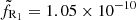 and
and  , are assumed to remain constant throughout the full cycle and were chosen to best fit radio observations at νR = 9 GHz. Strikingly, the global trends follow the observations reasonably well, with a net radio decrease (increase) near the switch-off (switch-on) phase in both cases. Clearly, the level of radio emission is always adjustable through the renormalisation factor
  . The shape of the light curve itself is noteworthy here, however, because again it is obtained using only constraints (rJ,ṁin) derived from X-ray spectra. This result is promising because reproducing the radio fluxes was not a requirement of our fitting procedure.
There are, however, some quantitative differences that deserve some attention. The theoretical radio flux is overestimated in the rising hard state by up to two orders of magnitude (upper triangles, days 0–80). This is especially the case for FR1 because it depends more strongly on the transition radius rJ. The same problem arises in the decaying phase, when the flux is underestimated at first (days 360–380) and overestimated later in the hard state (days 400–450). Most of these points belong to the 5% error-bar regions (or confidence intervals) for rJ, however. The fact that observed points always lie within these regions means that a reasonable radio light curve can be built using values of rJ(t) that are derived using the X-rays, even at epochs when X-rays are barely sensitive to rJ (largest error bars). Moreover, when the uncertainties in rJ decrease (blue zone), the model adequacy for the radio increases significantly. Because error bars in radio are quite small, explaining the radio emission during the hard states would only require changing rJ accordingly, with no significant loss of information in the X-rays. In practice, this discussion advocates the inclusion of radio luminosities within the fitting procedure, as described in Sect. 4.
A different kind of discrepancy between the radio emission models and data can be seen during the yellow soft-intermediate phases. In the high phase (days 100–130) the transition radius has not yet decreased to rin (corresponding to a zero-extent jet), and according to both our formulae, radio emission should be produced and detected. However, no detection of steady jets is reported, only flares (see Fig. 2). In the low phase (days 350–380), radio emission is detected at a level that is sometimes higher than predicted by the model (especially for FR1). Our simple jet emission model therefore seems to introduce significant errors during these phases. However, they correspond to rJ varying between rin and 2rin (Fig. 4). Now, the jet emission model assumes that the radio emission properties scale with the JED radial extent. It is doubtful that this would still hold when rJ → rin. Jet collimation properties (and possibly particle acceleration efficiency) may indeed undergo significant changes when the jet-launching zone becomes a point-like source. We should therefore not expect too much from our radio emission model during these states.
To summarize, our simple radio emission model does seem to predict the global trend for the observed radio light curve for both formulae. This was a byproduct of our JED-SAD formalism and not a requirement of the model. However, not only does the theoretical dependency of FR1 with rJ appears dubious, it is also less effective in reproducing the observed radio light curve. In the following, we therefore only focus on FR2.
4. Replication of the 2010–2011 cycle including radio constraints
4.1. Fitting procedure B
Hereafter, the radio flux is described by Eq. (3), and FR2 and  are now referred to as FR and
  . Because it is very sensitive to the transition radius rJ, this radio flux can thus be used along with the X-rays to constrain the disk dynamical state. For each observation at any given time, we therefore now search for the best pair (rJ,ṁin) that minimizes the new function
![Mathematical equation: $$ \begin{aligned} \zeta _{\rm X+R} = \zeta _{\rm X} + \frac{ | \text{ log} \left[ F_{\rm R} / F_{\rm R}^\mathrm{obs} \right] | }{\alpha _{\rm R}} ,\end{aligned} $$](/articles/aa/full_html/2019/06/aa35060-19/aa35060-19-eq16.gif) (4)
(4)
where ζX is defined in Eq. (1), FR is the predicted radio luminosity computed above,  the observed luminosity, and αR = 5 the radio weight chosen for best results. However, the addition of the radio constraints is not straightforward for the three following reasons:
-
(1)
We only have 35 radio observations across the ∼450 days of the observed cycle. Because no radio flux associated with compact jets has been observed during most of the soft-intermediate states (yellow) and during the soft state (red), no radio constraint will be imposed during these states (see Fig. 2). We thus use the former ζX (Eq. (1)) in these cases.
-
(2)
When they exist (hard and hard-intermediate states), radio observations often do not exactly match the date of X-ray observations. However, during these states, thanks to the high density of radio observations, we were able to interpolate radio observations and to associate an expected radio flux with each X-ray observation.
-
(3)
Theoretical radio fluxes FR are computed with Eq. (3) using the same normalization factor for the entire cycle. This is justified as long as some self-similar process is involved throughout the cycle. Contrary to the fitting procedure A, including the radio introduces a global constraint through this common value
 . Within procedure A, the radio light curve could be shifted vertically (in flux) by changing the value of
  without modifying either rJ or ṁin. In procedure B, the value of
  is included in each individual fit and thus influences the convergence to the best (rJ,ṁin) parameter set. Our best value is
  (we recall that rin = 2 here).
4.2. Results
Figure 7 shows the results of the fitting procedure B using both X-rays and radio fluxes. In comparison to procedure A, this new procedure introduces modifications to the transition radius rJ and marginally to the disk accretion rate ṁin. This leads to significant modifications to the radio flux FR and the spectral index Γ. To show these changes more clearly, we overplot the results from procedure A in gray lines in Fig. 7. As expected, the global X-ray flux and power-law fraction are not altered by the addition of radio constraints. Their evolution as well as the associated DFLD remain the same as in Fig. 3. The strongest quantitative modifications to the global evolution of rJ and ṁin occur in the hard states (Fig. 7, two bottom left panels). Instead of monotonically decreasing in time (as with procedure A), the transition radius now remains roughly stable around rJ ≃ 20 = 10rin, within most of the hard-state evolution and especially in the rising phase between days 0 and 80. This stability is consistent with previous calculations using the calculations made by Heinz & Sunyaev (2003), where rJ was not taken into account in the model. The smaller transition radius also leads to a slightly lower accretion rate, because the SAD (Paper III) has a higher radiative efficiency.
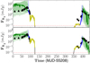 |
Fig. 6. Radio light curves at 9 GHz in mJy predicted using Eq. (2) (top) and Eq. (3) (bottom). The red dashed line at 10−2 mJy illustrates a typical detection limit. Markers correspond to observed radio fluxes associated with steady jets (see Fig. 2). |
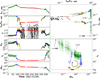 |
Fig. 7. 2010–2011 outburst of GX 339-4, derived using the fitting procedure B that takes into account X-rays and radio constraints. On the left, from top to bottom, light curves of 3–200 keV flux (in Eddington units), power-law fraction, power-law index, radio flux FR (in mJy), transition radius rJ, and accretion rate ṁin. Light curves of the same quantities, but obtained using procedure A (Fig. 3), are also reported with gray lines for comparison. On the right, evolutionary tracks in the associated DFLD (top) and in an rJ(ṁin)-diagram (bottom), in which the starting and ending positions are indicated. The color code is the same as previously: green triangles for the hard state, blue circles for the hard-intermediate, yellow crosses for the soft-intermediate, and red crosses for the soft state. Different symbols were used for the two phases of the hard state to better distinguish them: Upper triangles are used for the rising phase and lower triangles for the decaying phase. Error bars for the 5% and 10% confidence intervals are also displayed in the bottom right panel. |
Spectrally, the reproduction of the power-law index Γ is slightly degraded in the rising hard states (days 0–80). The other portions of the outburst are not affected because there is no radio constraint, and their reproduction remains satisfactory. In the hard states, the addition of a radio constraint forces a smaller transition radius than before (Fig. 7, left column, fifth panel). This results in spectra that are harder than those observed, with Γ ≃ 1.6−1.7 as compared to Γobs ≃ 1.5−1.6 (third panel). As argued in Sect. 3.1, this discrepancy could be easily compensated for by taking the reflection component better into account. Moreover, although our model deals with the illumination by the inner JED of the outer soft SAD photons, it does so in a quite simplified way using a simple geometrical factor ω. As shown for instance in Fig. 2 in Paper III, a slight modification of ω could lead to variations of up to 0.4 in Γ. The systematic error induced by these two simplifications has the correct order of magnitude to explain the discrepancies shown in Fig. 7. Therefore, the model is consistent with observations for the whole cycle.
Finally, and by construction, the addition of the radio fluxes within the fitting procedure allowed us to reproduce the radio light curve much better (Fig. 7, left column, fourth panel). The rising and decaying radio emissions during the hard states (green) now match almost perfectly. The hard-intermediate states (blue), during which a swift decrease or increase in radio luminosity occurs, are also recovered well. With no surprise, as with procedure A, the behavior of our jet emission model during the soft-intermediate states (yellow) has room for improvement: too much emission is predicted in high states. This issue was discussed in Sect. 3.2.2.
The bottom right panel in Fig. 7 shows the coevolution rJ(ṁin) of the disk accretion rate and the JED-SAD transition radius. The overall behavior qualitatively follows what was expected from previous theoretical works from Meyer-Hofmeister et al. (2005) or Kylafis & Belloni (2015), for example. These were only illustrations, whereas our rJ(ṁin) curve relies on complex modeling and fits performed on multiwavelength data. This representation suggests that the disk accretion rate is the only control parameter that leads to the observed evolutionary track of XrBs. This is not a conclusion that can be drawn yet. rJ indeed depends on the local disk magnetization (hence a function of the local magnetic field and disk column density), while ṁin depends on both the dominant torque and column density. There are thus two local disk quantities that come into play: the magnetic field and the column density; and the way the magnetic field evolves in accretion disks is still a pending question. One possible way to solve this question would be to determine how generic the resulting rJ(ṁin) curve is, for instance, by deriving it for all cycles of a given object as well as for different objects.
4.3. Open questions
Before concluding, a few open questions about our JED-SAD paradigm need to be discussed. In this section the production of Blandford & Znajek (1977) jets, the possible presence of winds, and the production of timing properties are considered.
First, in our view, jets are mainly emitted directly from the disk, that is, the inner JED portion, and we only computed the radio emission from that component. Because the global scenario from Paper I relies on the existence of a large-scale vertical magnetic field, jets emitted from the rotating black-hole ergosphere are also probably present (Blandford & Znajek 1977; Tchekhovskoy et al. 2011; McKinney et al. 2012). We did not take this dynamical component into account, and doing so might lead to some quantitative changes in the total radio emission. This deserves further investigation. Moreover, multiple radiative processes concerning the two jets have been ignored. We aim here at giving a first-order estimate of the jet contribution, but a more precise description of the radiative emission signature of the jets would lead to a more realistic picture. Effects such as jet collimation or inclination might be included, for instance. This work will be done by coupling our code with the jet spectral code ISHEM (Malzac 2014; Péault et al. 2019), and thus will also further address the possibility of dark jets (Drappeau et al. 2017). Additionally, our face-on disk is inconsistent with our edge-on estimates of the jet emission: this discrepancy will be solved in the future.
Second, another aspect that has been disregarded in our study so far is the possible production of winds. In X-ray binaries, winds have mainly been detected in the soft state (Lee et al. 2002; Ponti et al. 2012), but very recent work suggests the discovery of such winds in the hard state, which challenges this common and historical view (see, e.g., Homan et al. 2016; Tetarenko et al. 2018; Mata Sánchez et al. 2018). Unless, of course, the mass-loss rate in the wind is huge, the presence of such winds in the soft state would not have an important effect on the disk structure, and thus on the spectral shape in X-rays (see Paper III, Sect. 2.1.2). Their effect in the case of magnetically dominated (JED) disks remains to be investigated, however. It remains to be determined whether these winds are being launched below rJ, that is, within the JED portion of the disk. If this is confirmed, then a very interesting question arises: are these winds only the radiative signature of the base of the jets (low velocity and still massive outflow) or another, different, dynamical component making the transition from the outer standard accretion disk to the innermost jet-emitting disk? Although these observations do not involve GX 339-4, this question requires investigations in the future.
Last but not least, although timing properties are an important feature in the behavior of X-ray binaries, we did not discuss them here. Investigating hard-soft lags (see Uttley et al. 2014, for a recent review) and quasi-periodic oscillations (QPOs, see Zhang 2013; Motta 2016) requires us to consider the details of each observed spectrum. Such studies are beyond the scope of this paper. Our view is consistent with multiple timing properties, however. First, an abrupt transition in disk density is a highly favorable place for the productions of QPOs within different mecanisms. Such a radius could be associated with the location of some specific instability (Tagger & Pellat 1999; Varnière et al. 2012), the transition from the outer optically thick to the inner optically thin accretion flow (e.g., Giannios & Spruit 2004), or the outer radius of the inner ejecting disk (e.g., Cabanac et al. 2010). Investigations will be presented in a forthcoming paper. However, whether such a high-density break is stable and produces QPOs is a question that needs to be addressed. We note, for instance, that high-frequency QPOs are indeed observed in 3D general relativistic MHD simulations, at the radial transition between the inner magnetically arrested disks (MAD) or magnetically choked accretion flows (MCAF) and the outer standard accretion disk (see McKinney et al. 2012, and references therein). We also expect such a situation to arise in our case because the magnetic properties of MAD and MCAF are very similar to that of the jet-emitting disk: a vertical magnetic field near equipartition, near-Keplerian accretion (beyond the plunging region), and a global accretion torque caused by outflows. Second, while the production of time lags is usually associated with a corona or lampost geometry (Uttley et al. 2014, Fig. 1), very recent studies have shown that a radial stratification of the disk can be used to explain timing properties (Mahmoud & Done 2018; Mahmoud et al. 2019). This is very promising and fits surprisingly well with our own framework. These two timing questions will be raised and further studied in forthcoming works using dedicated observations.
5. Conclusion
Using the jet-emitting disk and standard accretion disk (JED–SAD) description for the inner regions of XrBs, we were able to replicate several observational diagnostics throughout the whole 2010–2011 cycle of GX 339-4 to a very good agreement. These diagnostics are the 3–200 keV total luminosity L3−200, the power-law luminosity fraction PLf = Lpl/L3−200, and the power-law index Γ. The observational X-ray constraints presented in this paper were derived from the RXTE/PCA observations of GX 339-4. The spectral parameters we used were provided by Clavel et al. (2016) and directly compared to the theoretical parameters. The theoretical parameters were obtained following the methods and limitations described in Papers II and III. The unknown dynamical parameters, allowed to vary throughout the cycle, are the JED–SAD transition radius rJ and the disk accretion rate onto the black hole ṁin.
Our present work followed a three-step process. We first searched for the best (rJ,ṁin) light curves that could reproduce all X-ray diagnostics. We then showed, using a simple self-absorbed synchrotron emission model for the jet, that the model predicts a radio light curve that is qualitatively consistent with the Corbel et al. (2013a) observations of GX 339-4 at that same epoch. We realized that radio observations introduce a strong constraint on the JED–SAD transition radius rJ during hard states, a constraint that is much more stringent than that provided by the X-ray data alone. As a last step, the radio luminosity was therefore included in the fits to constrain the disk dynamical state (rJ,ṁin) in accordance with the spectral shape in X-rays. This procedure greatly improved the agreement between the model and the radio observations, mostly by changing the magnitude and temporal behavior of rJ. Obviously, the parameters derived from X-ray observations can be strongly dependent on the spectral model that is selected and on the analysis procedures. We estimated the systematic errors that were introduced, in particular, those due to the reflection component that is not yet included in our model. They are found to be consistent with the small discrepancies between the model and observations. We are therefore confident of the robustness of our results, namely that the full XrB outburst and the trends derived for the model parameters rJ and ṁin are reproduced.
In order to fully understand the behavior of an outbursting XrB, the X-ray spectral changes and radio emission properties need to be explained. A full cycle therefore draws a trajectory in a 3D space, made of the DFLD plus the radio flux axis. Ultimately, our approach can be thought of as an effort to map this 3D evolutionary track into a 2D plot rJ(ṁin). If a figure such as presented in the bottom right panel of Fig. 7 indeed appears to be generic for a given object, then a dynamical explanation needs to be proposed. It will be a complex task because the evolution timescales involved are extremely long compared to any local timescale.
Acknowledgments
We thank the anonymous referee and Joey Neilsen for their helpful comments and careful reading of the manuscript. The authors acknowledge funding support from the French research national agency (CHAOS project ANR-12-BS05-0009, http://www.chaos-project.fr), the Centre National d’Etudes Spatiales (CNES), and the Programme National des Hautes Energies (PNHE). This research has made use of data, software, and/or web tools obtained from the high-energy astrophysics science archive research center (HEASARC), a service of the astrophysics science division at NASA/GSFC. Figures in this paper were produced using the MATPLOTLIB package (Hunter 2007).
References
- Begelman, M. C., & Armitage, P. J. 2014, ApJ, 782, L18 [NASA ADS] [CrossRef] [Google Scholar]
- Belmont, R. 2009, A&A, 506, 589 [NASA ADS] [CrossRef] [EDP Sciences] [Google Scholar]
- Belmont, R., Malzac, J., & Marcowith, A. 2008, A&A, 491, 617 [NASA ADS] [CrossRef] [EDP Sciences] [Google Scholar]
- Blandford, R. D., & Königl, A. 1979, ApJ, 232, 34 [NASA ADS] [CrossRef] [Google Scholar]
- Blandford, R. D., & Payne, D. G. 1982, MNRAS, 199, 883 [NASA ADS] [CrossRef] [Google Scholar]
- Blandford, R. D., & Znajek, R. L. 1977, MNRAS, 179, 433 [NASA ADS] [CrossRef] [Google Scholar]
- Bradt, H. V., Braes, L. L. E., Forman, W., et al. 1975, ApJ, 197, 443 [NASA ADS] [CrossRef] [Google Scholar]
- Cabanac, C., Henri, G., Petrucci, P. O., et al. 2010, MNRAS, 404, 738 [NASA ADS] [CrossRef] [Google Scholar]
- Casse, F., & Ferreira, J. 2000, A&A, 361, 1178 [NASA ADS] [Google Scholar]
- Casse, F., & Keppens, R. 2002, ApJ, 581, 988 [NASA ADS] [CrossRef] [Google Scholar]
- Clavel, M., Rodriguez, J., Corbel, S., & Coriat, M. 2016, Astron. Nachr., 337, 435 [NASA ADS] [CrossRef] [Google Scholar]
- Corbel, S., Nowak, M. A., Fender, R. P., Tzioumis, A. K., & Markoff, S. 2003, A&A, 400, 1007 [NASA ADS] [CrossRef] [EDP Sciences] [Google Scholar]
- Corbel, S., Fender, R. P., Tomsick, J. A., Tzioumis, A. K., & Tingay, S. 2004, ApJ, 617, 1272 [NASA ADS] [CrossRef] [Google Scholar]
- Corbel, S., Coriat, M., Brocksopp, C., et al. 2013a, MNRAS, 428, 2500 [NASA ADS] [CrossRef] [Google Scholar]
- Corbel, S., Aussel, H., Broderick, J. W., et al. 2013b, MNRAS, 431, L107 [NASA ADS] [CrossRef] [Google Scholar]
- Dauser, T., Garcia, J., Parker, M. L., Fabian, A. C., & Wilms, J. 2014, MNRAS, 444, L100 [NASA ADS] [CrossRef] [Google Scholar]
- Done, C., Gierliński, M., & Kubota, A. 2007, A&ARv, 15, 1 [NASA ADS] [CrossRef] [EDP Sciences] [Google Scholar]
- Drappeau, S., Malzac, J., Coriat, M., et al. 2017, MNRAS, 466, 4272 [NASA ADS] [Google Scholar]
- Dunn, R. J. H., Fender, R. P., Körding, E. G., Belloni, T., & Cabanac, C. 2010, MNRAS, 403, 61 [NASA ADS] [CrossRef] [Google Scholar]
- Eddington, A. S. 1926, The Internal Constitution of the Stars (Cambridge: Cambridge University Press) [Google Scholar]
- Esin, A. A., McClintock, J. E., & Narayan, R. 1997, ApJ, 489, 865 [NASA ADS] [CrossRef] [Google Scholar]
- Fender, R. P., Belloni, T. M., & Gallo, E. 2004, MNRAS, 355, 1105 [NASA ADS] [CrossRef] [Google Scholar]
- Fender, R. P., Homan, J., & Belloni, T. M. 2009, MNRAS, 396, 1370 [NASA ADS] [CrossRef] [Google Scholar]
- Ferreira, J. 1997, A&A, 319, 340 [Google Scholar]
- Ferreira, J., & Pelletier, G. 1993, A&A, 276, 625 [NASA ADS] [Google Scholar]
- Ferreira, J., & Pelletier, G. 1995, A&A, 295, 807 [NASA ADS] [Google Scholar]
- Ferreira, J., Petrucci, P. O., Henri, G., Saugé, L., & Pelletier, G. 2006, A&A, 447, 813 [NASA ADS] [CrossRef] [EDP Sciences] [Google Scholar]
- Galeev, A. A., Rosner, R., & Vaiana, G. S. 1979, ApJ, 229, 318 [NASA ADS] [CrossRef] [Google Scholar]
- Gallo, E., Fender, R. P., & Pooley, G. G. 2003, MNRAS, 344, 60 [NASA ADS] [CrossRef] [Google Scholar]
- García, J., Dauser, T., Lohfink, A., et al. 2014, ApJ, 782, 76 [NASA ADS] [CrossRef] [Google Scholar]
- García, J. A., Steiner, J. F., McClintock, J. E., et al. 2015, ApJ, 813, 84 [NASA ADS] [CrossRef] [Google Scholar]
- Giannios, D., & Spruit, H. C. 2004, A&A, 427, 251 [NASA ADS] [CrossRef] [EDP Sciences] [Google Scholar]
- Gierliński, M., Zdziarski, A. A., Poutanen, J., et al. 1999, MNRAS, 309, 496 [NASA ADS] [CrossRef] [Google Scholar]
- Heida, M., Jonker, P. G., Torres, M. A. P., & Chiavassa, A. 2017, ApJ, 846, 132 [NASA ADS] [CrossRef] [Google Scholar]
- Heinz, S., & Sunyaev, R. A. 2003, MNRAS, 343, L59 [NASA ADS] [CrossRef] [Google Scholar]
- Hjellming, R. M., & Wade, C. M. 1971, ApJ, 168, L21 [NASA ADS] [CrossRef] [Google Scholar]
- Homan, J., & Belloni, T. 2005, Ap&SS, 300, 107 [NASA ADS] [CrossRef] [Google Scholar]
- Homan, J., Neilsen, J., Allen, J. L., et al. 2016, ApJ, 830, L5 [NASA ADS] [CrossRef] [Google Scholar]
- Hunter, J. D. 2007, Comput. Sci. Eng., 9, 90 [NASA ADS] [CrossRef] [Google Scholar]
- Hynes, R. I., Steeghs, D., Casares, J., Charles, P. A., & O’Brien, K. 2003, ApJ, 583, L95 [NASA ADS] [CrossRef] [Google Scholar]
- Hynes, R. I., Steeghs, D., Casares, J., Charles, P. A., & O’Brien, K. 2004, ApJ, 609, 317 [NASA ADS] [CrossRef] [Google Scholar]
- Ichimaru, S. 1977, ApJ, 214, 840 [NASA ADS] [CrossRef] [Google Scholar]
- Körding, E. G., Jester, S., & Fender, R. 2006, MNRAS, 372, 1366 [NASA ADS] [CrossRef] [Google Scholar]
- Kylafis, N. D., & Belloni, T. M. 2015, A&A, 574, A133 [NASA ADS] [CrossRef] [EDP Sciences] [Google Scholar]
- Lasota, J. P., Narayan, R., & Yi, I. 1996, A&A, 314, 813 [NASA ADS] [Google Scholar]
- Lee, J. C., Reynolds, C. S., Remillard, R., et al. 2002, ApJ, 567, 1102 [NASA ADS] [CrossRef] [Google Scholar]
- Liska, M. T. P., Tchekhovskoy, A., & Quataert, E. 2018, ArXiv e-prints [arXiv:1809.04608] [Google Scholar]
- Ludlam, R. M., Miller, J. M., & Cackett, E. M. 2015, ApJ, 806, 262 [NASA ADS] [CrossRef] [Google Scholar]
- Mahmoud, R. D., & Done, C. 2018, MNRAS, 480, 4040 [NASA ADS] [CrossRef] [Google Scholar]
- Mahmoud, R. D., Done, C., & De Marco, B. 2019, MNRAS, 486, 2137 [NASA ADS] [CrossRef] [Google Scholar]
- Malzac, J. 2014, MNRAS, 443, 299 [NASA ADS] [CrossRef] [Google Scholar]
- Marcel, G., Ferreira, J., Petrucci, P. O., et al. 2018a, A&A, 615, A57 [NASA ADS] [CrossRef] [EDP Sciences] [Google Scholar]
- Marcel, G., Ferreira, J., Petrucci, P. O., et al. 2018b, A&A, 617, A46 [NASA ADS] [CrossRef] [EDP Sciences] [Google Scholar]
- Markert, T. H., Canizares, C. R., Clark, G. W., et al. 1973a, ApJ, 184, L67 [NASA ADS] [CrossRef] [Google Scholar]
- Markert, T. H., Clark, G. W., Lewin, W. H. G., Schnopper, H. W., & Sprott, G. F. 1973b, Int. Astron. Union Circ., 2483, 1 [NASA ADS] [Google Scholar]
- Mata Sánchez, D., Muñoz-Darias, T., Casares, J., et al. 2018, MNRAS, 481, 2646 [NASA ADS] [CrossRef] [Google Scholar]
- McKinney, J. C., Tchekhovskoy, A., & Blandford, R. D. 2012, MNRAS, 423, 3083 [NASA ADS] [CrossRef] [Google Scholar]
- Meyer-Hofmeister, E., Liu, B. F., & Meyer, F. 2005, A&A, 432, 181 [NASA ADS] [CrossRef] [EDP Sciences] [Google Scholar]
- Miller, J. M., Reynolds, C. S., Fabian, A. C., et al. 2008, ApJ, 679, L113 [NASA ADS] [CrossRef] [Google Scholar]
- Mirabel, I. F., & Rodríguez, L. F. 1998, Nature, 392, 673 [NASA ADS] [CrossRef] [Google Scholar]
- Motta, S., Belloni, T., & Homan, J. 2009, MNRAS, 400, 1603 [NASA ADS] [CrossRef] [Google Scholar]
- Motta, S. E. 2016, Astron. Nachr., 337, 398 [NASA ADS] [CrossRef] [Google Scholar]
- Muñoz-Darias, T., Casares, J., & Martínez-Pais, I. G. 2008, MNRAS, 385, 2205 [NASA ADS] [CrossRef] [Google Scholar]
- Murphy, G. C., Ferreira, J., & Zanni, C. 2010, A&A, 512, A82 [NASA ADS] [CrossRef] [EDP Sciences] [Google Scholar]
- Nandi, A., Debnath, D., Mandal, S., & Chakrabarti, S. K. 2012, A&A, 542, A56 [NASA ADS] [CrossRef] [EDP Sciences] [Google Scholar]
- Narayan, R., & Yi, I. 1994, ApJ, 428, L13 [NASA ADS] [CrossRef] [Google Scholar]
- Nokhrina, E. E., Beskin, V. S., Kovalev, Y. Y., & Zheltoukhov, A. A. 2015, MNRAS, 447, 2726 [NASA ADS] [CrossRef] [Google Scholar]
- Parker, M. L., Tomsick, J. A., Kennea, J. A., et al. 2016, ApJ, 821, L6 [NASA ADS] [CrossRef] [Google Scholar]
- Péault, M., Malzac, J., Coriat, M., et al. 2019, MNRAS, 482, 2447 [NASA ADS] [CrossRef] [Google Scholar]
- Petrucci, P.-O., Ferreira, J., Henri, G., & Pelletier, G. 2008, MNRAS, 385, L88 [NASA ADS] [CrossRef] [Google Scholar]
- Ponti, G., Fender, R. P., Begelman, M. C., et al. 2012, MNRAS, 422, L11 [NASA ADS] [CrossRef] [Google Scholar]
- Rees, M. J., Begelman, M. C., Blandford, R. D., & Phinney, E. S. 1982, Nature, 295, 17 [NASA ADS] [CrossRef] [Google Scholar]
- Reis, R. C., Fabian, A. C., Ross, R. R., et al. 2008, MNRAS, 387, 1489 [NASA ADS] [CrossRef] [Google Scholar]
- Remillard, R. A., & McClintock, J. E. 2006, ARA&A, 44, 49 [NASA ADS] [CrossRef] [Google Scholar]
- Rodriguez, J., Shaw, S. E., Hannikainen, D. C., et al. 2008, ApJ, 675, 1449 [NASA ADS] [CrossRef] [Google Scholar]
- Shakura, N. I., & Sunyaev, R. A. 1973, A&A, 24, 337 [NASA ADS] [Google Scholar]
- Tagger, M., & Pellat, R. 1999, A&A, 349, 1003 [NASA ADS] [Google Scholar]
- Tananbaum, H., Gursky, H., Kellogg, E., Giacconi, R., & Jones, C. 1972, ApJ, 177, L5 [NASA ADS] [CrossRef] [Google Scholar]
- Tchekhovskoy, A., Narayan, R., & McKinney, J. C. 2011, MNRAS, 418, L79 [NASA ADS] [CrossRef] [Google Scholar]
- Tetarenko, B. E., Sivakoff, G. R., Heinke, C. O., & Gladstone, J. C. 2016, ApJS, 222, 15 [NASA ADS] [CrossRef] [Google Scholar]
- Tetarenko, B. E., Lasota, J. P., Heinke, C. O., Dubus, G., & Sivakoff, G. R. 2018, Nature, 554, 69 [NASA ADS] [CrossRef] [Google Scholar]
- Tomsick, J. A., Kalemci, E., Kaaret, P., et al. 2008, ApJ, 680, 593 [NASA ADS] [CrossRef] [Google Scholar]
- Tzeferacos, P., Ferrari, A., Mignone, A., et al. 2013, MNRAS, 428, 3151 [NASA ADS] [CrossRef] [Google Scholar]
- Uttley, P., Cackett, E. M., Fabian, A. C., Kara, E., & Wilkins, D. R. 2014, A&ARv, 22, 72 [NASA ADS] [CrossRef] [EDP Sciences] [Google Scholar]
- Varnière, P., Tagger, M., & Rodriguez, J. 2012, A&A, 545, A40 [NASA ADS] [CrossRef] [EDP Sciences] [Google Scholar]
- Yuan, F., & Narayan, R. 2014, ARA&A, 52, 529 [NASA ADS] [CrossRef] [Google Scholar]
- Zanni, C., Ferrari, A., Rosner, R., Bodo, G., & Massaglia, S. 2007, A&A, 469, 811 [NASA ADS] [CrossRef] [EDP Sciences] [Google Scholar]
- Zdziarski, A. A., Gierliński, M., Mikołajewska, J., et al. 2004, MNRAS, 351, 791 [NASA ADS] [CrossRef] [Google Scholar]
- Zhang, S.-N. 2013, Front. Phys., 8, 630 [NASA ADS] [CrossRef] [Google Scholar]
All Figures
|
Fig. 1. Evolution of GX 339-4 during its 2010–2011 outburst in a 3–200 keV DFLD, showing the total L3−200 X-ray luminosity (in Eddington units) as a function of the power-law fraction. Hard states are displayed in green, hard-intermediate states in blue, soft-intermediate states in yellow, and soft states in red (see text). The five canonical states (Q, LH, HH, HS, and LS) defined in Paper III are highlighted by the black stars, and the observed approximate location of the jet-line is illustrated as a black line. Hard tail levels of 1, 3, and 10% are shown as red dotted, dashed, and solid lines, respectively (see text). |
| In the text | |
|
Fig. 2. Radio observations at 9 GHz during the 2010–2011 outburst of GX 339-4 (Corbel et al. 2013a,b). Steady jet emission is shown with triangle markers, upper for the rising phase and lower for the decaying phase, all corresponding to proper detections. Double arrows are drawn when radio emission was also observed but has been interpreted as radio flares or interactions with the interstellar medium (Corbel et al., in prep.). The vertical position of the arrows is arbitrary. The background color shades correspond to the X-ray spectral states (see Sect. 2.2). The epoch in white corresponds to a gap in the X-ray coverage due to solar constraints. |
| In the text | |
|
Fig. 3. Results of fitting procedure A applied to the 2010–2011 outburst of GX 339-4. The black markers are fits taken from Clavel et al. (2016) reported with their error bars when reliable, while color lines display our results: green, blue, yellow, and red for hard, hard-intermediate, soft-intermediate, and soft states, respectively (see Sect. 2). Left, from top to bottom: 3–200 keV total luminosity L3−200 (in Eddington units), the power-law luminosity fraction PLf = Lpl/L3−200, and the power-law index Γ. Right: DFLD. The hard tail proxy we used was frozen to 10%, but 1% and 3% proxies are also illustrated as red dot-dashed and dashed lines (see Paper III). |
| In the text | |
|
Fig. 4. Time evolution of rJ (top) and ṁin (down) associated with the best ζX defined by Eq. (1). The color code is the same as previously. The transparent colored areas correspond to the confidence intervals of 5% and 10% error margin (see text). |
| In the text | |
|
Fig. 5. Schematic view of the magnetized accretion-ejection structure as a function of radius r and altitude z. The extent of the JED and SAD is shown in gray (vertical heights were computed from our model, see Paper III), while the jet launched from the JED is shown in orange (sketch of what its geometry could look like). The photosphere rν(z) at a given frequency ν is shown in red, splitting the jet in an inner optically thick (dark orange) and outer optically thin (light orange) regions. Within our simple approach, each field line widens in a self-similar way so that at a given altitude z, a field line anchored at rin has achieved a radius r(z) = Wrin, while that anchored at rJ is WrJ, with the same asymptotic widening factor W. |
| In the text | |
|
Fig. 6. Radio light curves at 9 GHz in mJy predicted using Eq. (2) (top) and Eq. (3) (bottom). The red dashed line at 10−2 mJy illustrates a typical detection limit. Markers correspond to observed radio fluxes associated with steady jets (see Fig. 2). |
| In the text | |
|
Fig. 7. 2010–2011 outburst of GX 339-4, derived using the fitting procedure B that takes into account X-rays and radio constraints. On the left, from top to bottom, light curves of 3–200 keV flux (in Eddington units), power-law fraction, power-law index, radio flux FR (in mJy), transition radius rJ, and accretion rate ṁin. Light curves of the same quantities, but obtained using procedure A (Fig. 3), are also reported with gray lines for comparison. On the right, evolutionary tracks in the associated DFLD (top) and in an rJ(ṁin)-diagram (bottom), in which the starting and ending positions are indicated. The color code is the same as previously: green triangles for the hard state, blue circles for the hard-intermediate, yellow crosses for the soft-intermediate, and red crosses for the soft state. Different symbols were used for the two phases of the hard state to better distinguish them: Upper triangles are used for the rising phase and lower triangles for the decaying phase. Error bars for the 5% and 10% confidence intervals are also displayed in the bottom right panel. |
| In the text | |
Current usage metrics show cumulative count of Article Views (full-text article views including HTML views, PDF and ePub downloads, according to the available data) and Abstracts Views on Vision4Press platform.
Data correspond to usage on the plateform after 2015. The current usage metrics is available 48-96 hours after online publication and is updated daily on week days.
Initial download of the metrics may take a while.