| Issue |
A&A
Volume 656, December 2021
|
|
|---|---|---|
| Article Number | A45 | |
| Number of page(s) | 22 | |
| Section | Extragalactic astronomy | |
| DOI | https://doi.org/10.1051/0004-6361/202141143 | |
| Published online | 02 December 2021 | |
AGN feeding and feedback in Fornax A
Kinematical analysis of the multi-phase ISM⋆
1
INAF – Osservatorio Astronomico di Cagliari, via della Scienza 5, 09047 Selargius (CA), Italy
e-mail: This email address is being protected from spambots. You need JavaScript enabled to view it.
2
INAF – Osservatorio di Astrofisica e Scienza dello Spazio di Bologna, via Piero Gobetti 93/3, 40129 Bologna, Italy
3
Department of Astrophysical Sciences, Princeton University, 4 Ivy Lane, Princeton, NJ 08544-1001, USA
4
Institute of Astronomy, Graduate School of Science, The University of Tokyo, 2-21-1 Osawa, Mitaka, Tokyo 181-0015, Japan
5
Netherlands Institute for Radio Astronomy (ASTRON), Oude Hoogeveensedijk 4, 7991 PD Dwingeloo, The Netherlands
6
Kapteyn Astronomical Institute, University of Groningen, Landleven 12, 9747 AD Groningen, The Netherlands
7
Subaru Telescope, National Astronomical Observatory of Japan, National Institutes of Natural Sciences (NINS), 650 North A’ohoku Place, Hilo, HI 96720, USA
8
Department of Astronomical Science, The Graduate University for Advanced Studies, SOKENDAI, 2-21-1 Osawa, Mitaka, Tokyo 181-8588, Japan
9
Ruhr University Bochum, Faculty of Physics and Astronomy, Astronomical Institute, 44780 Bochum, Germany
10
Department of Physics, University of Pretoria, Private Bag X20, Hatfield 0028, South Africa
11
Department of Physics and Electronics, Rhodes University, PO Box 94 Makhanda 6140, South Africa
12
South African Radio Astronomy Observatory, 2 Fir Street, Black River Park, Observatory, Cape Town 7925, South Africa
Received:
20
April
2021
Accepted:
2
August
2021
Abstract
We present a multi-wavelength study of the gaseous medium surrounding the nearby active galactic nucleus (AGN), Fornax A. Using MeerKAT, ALMA, and MUSE observations, we reveal a complex distribution of the atomic (H I), molecular (CO), and ionised gas in its centre and along the radio jets. By studying the multi-scale kinematics of the multi-phase gas, we reveal the presence of concurrent AGN feeding and feedback phenomena. Several clouds and an extended 3 kpc filament – perpendicular to the radio jets and the inner disk (r ≲ 4.5 kpc) – show highly-turbulent kinematics, which likely induces non-linear condensation and subsequent chaotic cold accretion (CCA) onto the AGN. In the wake of the radio jets and in an external (r ≳ 4.5 kpc) ring, we identify an entrained massive (∼107 M⊙) multi-phase outflow (vOUT ∼ 2000 km s−1). The rapid flickering of the nuclear activity of Fornax A (∼3 Myr) and the gas experiencing turbulent condensation raining onto the AGN provide quantitative evidence that a recurrent, tight feeding and feedback cycle may be self-regulating the activity of Fornax A, in agreement with CCA simulations. To date, this is one of the most in-depth probes of such a mechanism, paving the way to apply these precise diagnostics to a larger sample of nearby AGN hosts and their multi-phase inter stellar medium.
Key words: galaxies: individual: Fornax A / galaxies: individual: NGC 1316 / galaxies: active / galaxies: kinematics and dynamics / galaxies: ISM / accretion / accretion disks
Reduced images and datacubes are also available at the CDS via anonymous ftp to cdsarc.u-strasbg.fr (130.79.128.5) or via http://cdsarc.u-strasbg.fr/viz-bin/cat/J/A+A/656/A45
© ESO 2021
1. Introduction
Feedback from active galactic nuclei (AGNs) is one of the key processes that can affect the evolution of a galaxy. The energy released by the supermassive black hole (SMBH) as radiation and/or jets of radio plasma induces disturbances in the hot halo of its host galaxy, generating cavities and shocks that prevent the hot gas from cooling (Fabian 2012; McNamara & Nulsen 2012; Baldi et al. 2019). The energy of AGNs is sufficient to quench star formation and cooling flows in massive galaxies and groups and clusters (Churazov et al. 2012; Cano-Díaz et al. 2012; Carniani et al. 2016; McDonald et al. 2018), mainly through the ejection of jets and circulation of massive gaseous outflows (see, for example, King & Pounds 2015; Harrison 2017; Morganti & Oosterloo 2018; Veilleux et al. 2020, for different reviews on the topic).
In some models of galaxy evolution, multiple feedback episodes are needed to prevent cooling from the hot halo and efficiently regulate star-formation (see, for example, Ciotti et al. 2010; Gaspari et al. 2017; Prieto et al. 2021). Since AGNs are associated with the accretion of material onto the SMBH, recurrent feedback is generated by recurrent accretion events (i.e., recursive feeding). The existence of recurrent AGNs has long been known (e.g., Cordey 1987; Saikia & Jamrozy 2009; Shulevski et al. 2017; Brocksopp et al. 2007; Orrù et al. 2015). Recently, low-frequency radio surveys have shown that multiple phases of activity occur in a non-negligible number of sources (Sabater et al. 2019; Morganti et al. 2021), and short timescales of activity, between 1 and 100 Myr, were derived (Brienza et al. 2017; Sabater et al. 2019).
Multi-wavelength spectral observations are essential for a complete characterisation of feeding and feedback phenomena. High-resolution observations of the kinematics of the gas are crucial to distinguishing between feeding (i.e., inflows of gas) and feedback processes (i.e., gaseous outflows).
Gaseous outflows are known to be multi-phased, from the hot, highly ionised phase (T ≳ 106 − 8 K; e.g., Tombesi et al. 2013), to the warm ionised (T ∼ 103 − 6 K; e.g., Mingozzi et al. 2019; Davies et al. 2020), neutral-atomic (T ∼ 102 − 3 K; e.g., Morganti & Oosterloo 2018; Roberts-Borsani & Saintonge 2019), and molecular phase (T ≲ 102 K e.g., Fluetsch et al. 2021; Veilleux et al. 2020). A tight correlation between the distribution and kinematics of these gaseous phases has been observed in several galaxies (see, for example, NGC 1266, Mrk 231, IC 5063 in Alatalo et al. 2011; Veilleux et al. 2016; Oosterloo et al. 2019, respectively), with the cold neutral gas seemingly the most massive (Cicone et al. 2018; Fluetsch et al. 2021; Veilleux et al. 2020).
In self-regulated feedback scenarios, outflows inject turbulence into the surrounding medium, causing the hot gas to condense from the hot phase into cold-atomic and then molecular clouds, which then ‘rain’ back down, growing the central SMBH (Gaspari et al. 2019). In a handful of galaxies, both feeding and feedback processes have been associated with the same episode of activity (see, for example NGC 1433, NGC 1068 and NGC1808 in Combes et al. 2013; García-Burillo et al. 2019; Audibert et al. 2021, respectively), but a connection with a previous (or future) activity and the sustainability of recursive triggering has not been made.
Chaotic cold accretion (CCA; Gaspari et al. 2013, 2015, 2017; King & Nixon 2015; Prasad et al. 2017) is one of the few major feeding mechanisms that can generate rapid recursive nuclear activity, self-consistently. In this process, cold clouds and filaments condense out of the hot phase via turbulent, non-linear thermal instability. Chaotic collisions promote the ‘funneling’ of the cold phase towards the SMBH and ignite the AGN (Gaspari et al. 2012; Yang et al. 2019). Feedback from the AGN outflows re-heat the core, while entraining the ambient gas, establishing a tight AGN self-regulated loop (Gaspari 2017). Hence, linking chaotic accretion to the cooling rate induces a natural self-regulation, with a flickering recursive cycle and peaks of AGN activity.
The CCA model provides key predictions for the kinematics of all phases of the gas, and the correlations between them, which can be directly compared with the results of multi-wavelength spectral observations (Gaspari et al. 2018). There is a range of evidence of cooling and inflows connected to CCA in the kinematics of several phases of the interstellar, intragroup, and intracluster media (H I, CO, Hα gas, and X-ray halos; Rose et al. 2019; Storchi-Bergmann & Schnorr-Müller 2019) and in different types of host galaxies, from isolated early-type galaxies (e.g., Maccagni et al. 2014, 2016, 2018; Lakhchaura et al. 2018) to group galaxies (see, for example, Temi et al. 2018; Juráňová et al. 2019, 2020) and brightest cluster galaxies (e.g., Tremblay et al. 2016, 2018; Olivares et al. 2019). However, it is challenging to trace this phenomenon from the macro-scale (tens of kpc) to the micro-scale (sub-pc) where the accretion onto the SMBH occurs (see Gaspari et al. 2020, for a review). So far, most detections trace in-falling gas in the innermost 100 pc, or average properties of the ∼1–20 kpc halo have been used to infer the presence of cooling caused by turbulence.
Recurrent nearby AGNs are ideal to study in detail feeding and feedback mechanisms, quantify their impact on the evolution of the galaxy and understand how they can self-regulate their recursive activity. Among these AGNs, the nearby (DL = 20.8 Mpc Cantiello et al. 2013) radio galaxy Fornax A is a pivotal target. The radio spectral distribution of Fornax A shows indications of rapid flickering (Maccagni et al. 2020). Its giant radio lobes suggest they formed through multiple episodes, the last of which was interrupted 200 Myr ago. More recently (∼3 Myr ago), a less powerful and short (1 Myr) phase of nuclear activity generated the central s-shaped jets, which are now expanding in the Inter-Stellar Medium (ISM). Currently, the core may be in a new active phase.
A major merger occurred 1–3 Gyr ago (e.g., Schweizer 1980; Serra et al. 2019). This event likely caused the first triggering of the radio source and brought large amounts of dust (Schweizer 1980; Lanz et al. 2010; Galametz et al. 2012; Duah Asabere et al. 2016), molecular gas (Horellou et al. 2001; Galametz et al. 2014; Morokuma-Matsui et al. 2019), and neutral hydrogen (Horellou et al. 2001; Serra et al. 2019; Richtler et al. 2020; Kleiner et al. 2021) into the centre and around the galaxy. Figure 1 shows that the dust seen in extinction in the innermost ≈8 kpc is distributed mainly in two structures: a stripe crossing the centre from the north-west to the south-east; and two outer arcs that seem to originate at the bend of the radio jets. Hα, CO, and H I are detected both on the stripe and along the outer arcs (Mackie & Fabbiano 1998; Morokuma-Matsui et al. 2019; Serra et al. 2019). The molecular gas shows clouds with irregular kinematics on both features, suggesting a tight interplay between the expansion of the radio jets and the surrounding interstellar medium (Morokuma-Matsui et al. 2019).
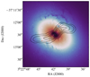 |
Fig. 1. Hubble ACS visible emission (535 nm) of the centre of Fornax A, radio jets seen by MeerKAT at 1.4 GHz are overlaid in black. Contour levels are 5 × 10−4 × 2n Jy beam−1 (n = 0, 1, 2, …) (Maccagni et al. 2020). |
In this paper, we analyse the kinematics of the multi-phase gas in NGC 1316 (Fornax A) in detail. We aim to understand if and how the cold and ionised gases triggered the nuclear activities in the last 3 Myr, and what the feedback effects resulting from these are. Section 2 describes the observations from state-of-the-art radio, millimetre, and optical telescopes to study the multi-phase gas in Fornax A at high spatial and spectral resolution. Sections 3 and 5 show the distribution, velocity field, and dispersion maps of the H I, CO and ionised gas detected in the innermost arcminute of the galaxy. The detailed analysis of their kinematics is discussed in Sect. 6. In Sect. 7, we reflect on how the AGN and its jets affect the gas kinematics, and, vice versa, how the gas may fuel the AGN and influence the expansion of the radio jets revealing the presence of both feeding and feedback phenomena. Section 8 summarises the most important results of this work.
2. Observations and data reduction
For the purposes of this paper we consider high resolution spectral observations from the radio, millimetre and optical wavelengths. We use MeerKAT observations to study the neutral hydrogen (H I) 21-cm line, the Atacama Large Millimeter and sub-millimeter Array (ALMA) for the 12CO(1−0) emission and the Multi Unit Spectroscopic Explorer (MUSE) on the Very Large Telescope (VLT) for the ionised lines (Balmer lines, [O III], [O I], [N II] and [S II]).
Even though these instruments are the ones producing the highest spectral and spatial resolutions in their respective bands, we point out that the spatial resolution of the MeerKAT and ALMA observations (∼20″) is ten times lower than the one of MUSE (∼2″), and their spectral resolution is between two and five times better. On the other hand, the MeerKAT H I and ALMA CO observations have a wide field of view (FoV; 1° and 8′, respectively), while MUSE observations are limited to the innermost arcminute of AGNs. Because of the proximity of Fornax A, the combination of all three observations allows us to study the interstellar medium (ISM) in detail from its innermost kilo-parsec to the periphery of its stellar body. In Table 1, we summarise the main properties of the MeerKAT, ALMA, and MUSE observations.
Main properties of the observations of the multi-phase gas in NGC 1316.
2.1. Neutral atomic hydrogen observations
We observed Fornax A with MeerKAT (Jonas & MeerKAT Team 2016; Camilo et al. 2018) in two different commissioning observations in June 2018. The observations were carried out with a different number of antennas (36 and 64, respectively) using the 4096-channels correlator set in the 856–1712 MHz frequency interval in full polarisation. The channel width is 209 kHz, corresponding to 44.5 km s−1 for H I at redshift z = 0. The total integration time on Fornax A was 8+7 hours.
A complete description of the data reduction of the 21-cm observations can be found in Kleiner et al. (2021). The data reduction was made with CARACal1 (Józsa et al. 2020). CARACal is a containerised pipeline written in Python3 and has been used to reduce several radio continuum and spectral observations from MeerKAT (e.g., Ramatsoku et al. 2020a; de Blok et al. 2020; Kleiner et al. 2021), the Very Large Array (Ramatsoku et al. 2020b), and the upgraded Giant Meterwave Radio Telescope (Michałowski et al. 2019).
For the purposes of this paper, we generated a datacube using a smaller arcsecond-tapering than the one used in Kleiner et al. (2021), which allowed us to obtain a higher spatial resolution of 22″ × 18″. The noise in the cube is 0.1 mJy beam−1 per channel. This corresponds to a 3σ H I column density sensitivity of 3.2 × 1019 cm−2 in a single channel, and to a surface brightness sensitivity limit of 0.25 M⊙ pc−2. Assuming a 100 km s−1 line width, the 5σ point-source MHI sensitivity is 3.0 × 10⁶ M⊙ at the assumed distance of 20.8 Mpc.
Since we knew of the presence of H I in the centre of Fornax A from previous MeerKAT observations (Serra et al. 2019), we fine-tuned the parameters of the source-finding algorithm SoFiA2 (Serra et al. 2015) to retrieve all the already-known H I and investigate the significant presence of a previously undetected and more diffuse component. The resulting surface brightness map, velocity field, and velocity-dispersion field are shown in Fig. 2.
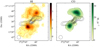 |
Fig. 2. Left panel: surface brightness map of the H I gas in the centre of Fornax A. Right panel: same maps for the 12CO(1−0). The PSF of all maps is at 22″ × 18″. Surface brightness contour levels are 3σ × 2n M⊙ pc−2 (n = 0, 1, 2, …) in all panels. The lowest contour corresponds to the 3σ surface brightness detection limit. Radio jets are the same as in Fig. 1. |
2.2. Molecular gas observations
A complete description of the reduction of the ALMA 108 GHz observation can be found in Morokuma-Matsui et al. (2019). The PSF of the resulting datacube is very asymmetric (15.5″ × 7″); hence, for a quantitative comparison between the atomic and molecular phase, we generated a new 12CO(1−0) datacube at the same spatial resolution of the H I. We created the total 12CO(1−0) image, velocity field, and velocity-dispersion field using SoFiA, analogously to what was done for the H I. We converted the brightness temperature map (TB, CO) in surface brightness units assuming a Galactic 12CO(1−0)-to-H2 conversion factor X2 = 4.3 M⊙(K km s−1 pc−2)−1. The noise in the datacube is 12 mJy beam−1 per channel (Δv ∼ 9.9 km s−1). This corresponds to a 3σ surface brightness limit of 0.33 M⊙ pc−2.
2.3. Ionised gas observations
To study the ionised gas in Fornax A, we selected two different sets of MUSE observations available in the ESO archive3. The wavelength coverage of the MUSE cubes ranges from 4650 Å to 9300 Å. Within this interval, MUSE achieves a resolution of R ∼ 1750–3750, which at the [N II]λ6583 line corresponds to approximately 68 km s−1.
The first dataset consists of four different observations of the full stellar body of Fornax A. These observations were taken on November 11, 2014 and December 13, 2014 (proj. ID: 094.B-0298, PI Walker, C.J.). The total integration time per observation is 333s. The spatial resolution of the observations given by the seeing is ≈2.1″.
In all datacubes, we detect the Balmer lines (Hα, Hβ) as well as the forbidden transitions of the ionised metals [O III]λ4959, [O III]λ5007, [O I]λ6300, [O I]λ6364, [N II]λ6548, [N II]λ6583, [S II]λλ6716,6731, and the NaI D absorption doublet of neutral gas. As available in the archive, the four mosaics of the single MUSE pointings have strong sky variations throughout the field of view. The low signal-to-noise of most detected lines does not allow a complete characterisation of their total flux and kinematical properties (i.e., line-shift and line-width). For this reason, we use this mosaic only to describe the overall kinematics of the ionised gas throughout the entire stellar body by focusing only on the [N II]λ6583 line (see Sect. 6).
To estimate and subtract the stellar continuum, we binned the datacubes using Voronoi tessellation to achieve an average signal-to-noise ratio (S/N) of 30 per wavelength channel in each bin between 4650 and 6800 Å. In this step, all spectra of the datacube with S/N ≲ 3 were discarded. This step is performed using the GISTpipeline4 (Bittner et al. 2019). The pipeline models the stellar continuum using the MILES stellar library templates (Sánchez-Blázquez et al. 2006), which covers the wavelength range from 3525–7500 Å. The fitting is performed using an adapted Penalized Pixel-Fitting routine (pPFX, Cappellari & Emsellem 2004; Cappellari 2017) and allowing an additive Legendre eleventh-order polynomial to correct for the shape of the continuum template.
We joined the four stellar-subtracted datacubes using Montage. From the mosaicked cube, we extracted a sub-cube centred on the [N II]λ6583 line in the velocity range [−2100, +800] km s−1 with respect to the systemic velocity of NGC 1316 (vsys = 1720 km s−1). In the rest of the paper, we refer to this datacube as the wide-field. MUSE datacube (of which the FoV is approximately 17.24 × 12.53 kpc).
Recently, Richtler et al. (2020) presented the same observations focusing on the [N II]λ6583 line and the NaI D absorption doublet. Our study presents both points of agreement and tension with the conclusions of these authors, as detailed in Sects. 6 and 7.
The second dataset consists of a deeper single pointing MUSE observation in the innermost arcminute of Fornax A. This observation was taken on July, 24th, 2018 (proj. ID: 0101.D-0748, PI K. Hanindyo) in four different exposures. The total integration time was 2178s over the spectral range 4750–9350 Å. The spatial resolution given by the seeing is ∼2.3″. We used the MUSE datacube available in the ESO archive (which has been produced using the MUSE pipeline v1.4 with default parameters; Weilbacher et al. 2014).
We subtracted the stellar continuum following the same procedure as for the wide-field datacube. In this observation, the [O III]λ5007 line is detected, on average, with S/N ∼ 5, when present. This allows us to avoid performing Voronoi binning on the stellar-subtracted datacube to reach a uniform S/N over the entire field of view. Instead, we only selected those pixels where the signal-to-noise ratio of the [O III]λ5007 is higher than 3.5. In the rest of the paper, we refer to this dataset as the centre-field datacube.
2.4. Estimate of the line emission parameters
In the centre-field datacube, we measured the main kinematical properties of the ionised gas by simultaneously fitting, on a pixel-by-pixel basis, one or two Gaussian components to the Hβ, [O III]λ5007, [O III]λ4959, [N II]λ6548, Hα, [N II]λ6583, and [S II]λλ6716,6731 lines (we excluded the low-S/N [O I] lines). In the simultaneous fit, each component was tied to have the same velocity centroid and dispersion in all lines, while the amplitudes are allowed to vary freely. The fits were performed using the Python library lmfit (Newville et al. 2014). lmfit provides non-linear optimisation and is built on the Levenberg-Marquardt algorithm. The fitting routine, computation of the residuals, as well as all outputs presented in this paper made use of the GuFo5 suite we developed.
Across the field of view, the emission lines show different properties. In some regions, they are narrow and single-peaked, in others they are shallow and broad, while in the centre they clearly show the presence of a significant second peak (see Appendix A for a collection of spectra). To choose the best-fit solution, we performed two different fitting runs. In the first run, we fitted a single Gaussian component, with dispersion that can vary between 1 and 1000 km s−1 and centroid that may range within ±700 km s−1 with respect to vsys. In the second run, we fitted two Gaussian components by letting the σ parameter of both components vary between 1 and 1000 km s−1.
In each run, for every line, we determined the residuals of the fits in the ±1200 km s−1 velocity interval centred on the systemic velocity of Fornax A. The best-fit solution minimises the residuals of the [O III]λ5007 line. One Gaussian component was sufficient to describe the emission lines in most of the field of view, except in the centre and in other regions along the nearly edge-on disk (see Sect. 5). For each line of sight (with S/N[OIII]λ5007 ≳ 3.5), we measured the following properties of each component and of the total fitted lines: flux, centroid, dispersion, and w80 (the width including 80% of the flux).
Overall, we performed the fit just described in ≈105 sight lines. To reduce computing time, we used the common multiprocess libraries of Python 3.
3. Distribution and kinematics of the cold gas
In Fig. 2, we show the distribution of the neutral and molecular gas seen at the same resolution (22″ × 18″) along with the radio jets of Fornax A. The cold gas extends out to 6.5 kpc in the north and 8.0 kpc in the south. Both the H I and 12CO(1−0) follow the dust distribution, mainly oriented nearly edge-on along the NS direction, with arcs at larger radii (r ≳ 4.5 kpc). The most prominent difference between the H I and the CO is that diffuse neutral hydrogen is also detected perpendicularly to the dust (in the NE-SW direction), while molecular gas is not. The H I also extends further out in the south of the field of view, but the sensitivity of ALMA in these regions is much lower than in the centre.
We use the relations shown in Meyer et al. (2017) to convert the flux density map into H I column density and surface brightness units. The total H I mass in the centre of Fornax A is ∼6.7 × 10⁷ M⊙. This is about 30% more than what was measured in Serra et al. (2019), indicating that a significant component of H I in Fornax A has low column densities (between 1 − 3 × 1019 cm−2).
From the integrated 12CO(1−0) line, we measure a total H2 = 5.8 × 10⁸ M⊙ (following the classical relations shown in, for example, Bolatto et al. 2013). The result is in agreement with what was measured by Morokuma-Matsui et al. (2019) and is comparable to previous single-dish observations (Wiklind & Henkel 1989; Sage & Galletta 1993; Horellou et al. 2001)
The velocity fields of the H I and CO are shown in Fig. 3. The kinematics of both phases of the cold gas are comparable. Exceptions are in the centre and perpendicularly to the jets in the NE, where blueshifted H I is detected but no CO is found.
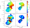 |
Fig. 3. Left panels: velocity and velocity dispersion fields of the H I gas in the centre of Fornax A. Right panels: same maps for the 12CO(1−0). The PSF of all maps is 22″ × 18″. Surface brightness contour levels and radio jets are the same as in Fig. 2. |
The moment-2 maps (bottom panels of Fig. 2) show that in most regions the velocity dispersion of both H I and CO gas are narrow (≲50 km s−1), as is normally found in galaxy disks. In both phases of the gas, the highest dispersion is found where the radio jets bend in the NW, and, more evidently, in the SE.
4. The H2/H I ratio
Figure 4 shows the H2/H I ratio distribution derived from the surface brightness maps. Green contours indicate a positive ratio, while orange contours show an over-abundance of H I, and the ratio is determined from the 3σ detection limit of the molecular gas. The integrated H2/H I ratio is ∼5.5, but this is given by averaging regions overabundant in molecular gas (as the outer arcs) with regions where only H I is found. The H2/H I map reveals that in the outer arcs the H2/H I peaks (as high as 10) correspond to the peaks of dust extinction. In the centre, along the nearly edge-on dust lane the H2/H I ratio is, on average, higher than in the outer arcs (6.8 and 3.5, respectively), while the regions perpendicular to the disk are depleted of H2and show ratios ≲1. Along the jets (mainly in the south) we find a sharp increase of the H2/H I ratio, while perpendicularly to the radio jets only H I is found. In these regions, the H I clouds also have very different projected velocities compared to the neighbouring regions (Fig. 3). These neutral gas clouds, with peculiar kinematics and no molecular counterpart, are also detected in the MUSE observations in the NaI D absorption doublet (Richtler et al. 2020).
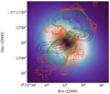 |
Fig. 4. Hubble ACS visible emission (535 nm) of the centre of Fornax A. Green solid contours show regions where the inferred H2 mass surface density is greater than the H I mass surface density (H2/H I ≳ 1), while orange dashed contours show regions rich in atomic hydrogen H I, but where H2 is not detected. The radio jets are shown in black. |
5. Distribution and moment maps of the ionised gas in the innermost arcminute
From the results of the simultaneous fitting of all detected emission lines (see Sect. 2.4), we build the total flux distribution maps for each line (Fig. 5). A visual inspection of Fig. 5 suggests that the emission lines are mainly low-ionisation nuclear emission-line region (LINER)-like, with notable exceptions in the centre and where the radio jets bend, where excitation appears to be more AGN-like. This paper focuses on the kinematics of the multi-phase gas; hence, we leave the discussion on the emission line ratios and excitation mechanisms to a following paper.
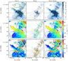 |
Fig. 5. Flux density distribution (top row), velocity field (central row), and velocity dispersion maps (bottom row) of the ionised gas. Left, middle, and right columns: distribution of the narrow Gaussian component, of the broad Gaussian component, and of the integrated fitted line (narrow+broad components), respectively. The radio jets of Fornax A are overlaid in grey in all panels. See Sect. 5 for details on the regions identified in the top left panel. |
The brightest line throughout the entire field of view is the [N II]λ6583. Since in the fitting procedure we constrained the centroid and width of all lines to be the same, we only show the properties of this line, which, in this study, is representative for all lines. In the top row of Fig. 5, we show the line decomposition in Gaussian components. While most emission can be described using a single Gaussian (shown in the left column), the presence of a second broader component (central column) is required in the centre, and along filaments oriented approximately east-west, in particular, where the radio jets bend. In the top left panel of the figure, we highlight three peculiar distributions of the gas. The first (A-line) follows the overall distribution of the dust and cold gas along the NW-SE direction. The second (B-line) is oriented east-west (PA = 80°) and has no observed dust or molecular gas counterpart. We refer to this feature as the EW stripe. Slightly to the north of this feature, we find several clouds of ionised gas with almost no dust (C-ellipse). These clouds coincide with the H I clouds with highly blueshifted velocities and no molecular counterpart. In Appendix A, we show different spectra extracted from the centre and these regions.
In the central row of Fig. 5, we show the velocity field of the ionised gas measured from the shift of the lines with respect to the systemic velocity of Fornax A (vsys = 1720 km s−1). In the right column, where we show the sum of the narrow and broad components (left and middle column, respectively), the centroid is the velocity position of the barycentre of the line. Overall, the NW-SE distribution of the ionised gas appears to be dominated by rotation, as suggested by the redshifted velocities in the NW and blueshifted ones in the SE, and follows the same kinematics as the cold gas (Fig. 3). Notable exceptions are the EW filaments in proximity of the radio jets. These are redshifted (vlos ≳ 350 km s−1) compared to the overall rotation of the neighbouring regions, and their molecular counterpart (see Fig. 2) was also previously identified as non-rotating (Morokuma-Matsui et al. 2019).
The EW-stripe is aligned with the major axis of the stellar body and is perpendicular to the dust lane, which may lead to misinterpretation of the nature of this feature as an edge-on, circumnuclear disk (e.g., Richtler et al. 2020), as seen in several active early-type galaxies (e.g., NGC 1813 and PKSB 1718-649; Krajnović et al. 2015; Maccagni et al. 2016, 2018, respectively). In Fornax A, however, the kinematics of the EW-stripe do not suggest that it can be an edge-on disk. The stripe has redshifted velocities in the east but does not show a blueshifted counterpart in the west. This is also visible in the single channel maps of the wide-field MUSE observations (see Sect. 6).
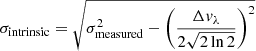
In the last row of Fig. 5, we show the velocity dispersion maps. To obtain the intrinsic dispersion of the line, we deconvolve the measured dispersion (σmeasured) by the spectral resolution of MUSE at the wavelength of the emission lines (Δvλ)6.
The broadest lines (σ ≳ 300 km s−1) are detected in the centre and along the radio jets, where either a single broad and shallow component or two Gaussians best describe the observed lines. In Sect. 7.2, we further discuss the presence of outflowing gas in these regions.
6. Analysis of the kinematics of the ISM in Fornax A
We study the kinematics of the multi-phase ISM over the entire stellar body of Fornax A (r ≲ 10 kpc) making use of the H I cube, 12CO(1−0) cube, and the [N II]λ6583 datacube extracted from the MUSE mosaic (Sect. 2). The moment maps of the H I and CO suggest that in the innermost arcminute (r ≲ 6 kpc), most gas rotates on a nearly edge-on disk. This is also supported by the appearance of the dust lane in the HST image (Fig. 1), where most of the gas seen in extinction is located on the eastern side, suggesting that it is the nearest side to us. In the left panel of Fig. 6, we show the position-velocity (pv-) diagram taken along the major axis of this disk (PA = −30°). The smooth velocity gradients of the H I and of the CO (left panel) confirm the overall rotation of the cold gas. Nevertheless, several clouds are deviating from the regular rotation both in the west and east side of the disk, as well as in the centre (previously identified in the moment maps, see Sect. 5.
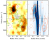 |
Fig. 6. Position-velocity diagrams along the major axis of the inner nearly edge-on disk. Left panel: Pv-diagram of the atomic and molecular gas (green contours). H I emission is shown by the colour scale and orange solid contours, while absorption is represented by dashed contours. Contour levels are −5; −3; 3, 5, 6, 12, 24σ. Right panel: Pv-diagram derived from the [N II]λ6583 emission (blue colour scale) overlaid with the H I emission and absorption. |
In the centre, H I is also detected in absorption in a single channel at the systemic velocity with optical depth of τ = 0.004 (which corresponds to NHI ∼ 3.0 × 1019cm−2, assuming a spin temperature of 100 K). The right panel of Fig. 6 shows the pv-diagram of the [N II]λ6583 line along the same axis, overlaid with the H I gas. Most of the ionised gas also follows the overall regular rotation of the cold gas. Nevertheless, strong deviations are present throughout the entire disk, and several clouds show counter-rotating velocities. In the centre, the dispersion of the ionised gas is maximum, suggesting that the nuclear activity is still perturbing the gas in the innermost regions.
Outside the innermost arcminute (r ≳ 6 kpc), the distribution of the ISM changes abruptly. The distribution of the dust (Fig. 1) shows the presence of a northern arc. The H I and CO gas follow the same arc and, therefore, cannot be co-planar with the inner, nearly edge-on disk. Furthermore, the velocity fields of the cold gas (top panels of Fig. 3) indicate that this arc is not just a more face-on extension of the inner disk because gas crosses the systemic velocity when moving from west to east along it (approximately between velocities 1600 and 2100 km s−1, see the emission marked by green and orange contours in Fig. 7); in the case of a simple inclination change, we would expect all gas in the northern arc to be redshifted, connecting in velocities with the northern edge of the inner disk.
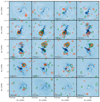 |
Fig. 7. Consecutive channel maps of the [N II]λ6583 line extracted from the MUSE wide-field datacube in the velocity range 1174 − 2400 km s−1 (the systemic velocity of Fornax A is 1720 km s−1). The contours of the CO emission (0.03, 0.06, 0.12, 0.15, 0.2 Jy beam−1) and of the H I gas (0.15, 0.3, 0.6, 1.2 mJy beam−1) are shown in green and orange, respectively. |
The information provided by the cold gas is limited, and we cannot know if the northern arc is part of a larger structure connecting the gas seen in the south-east of the inner disk. The ionised gas observations allow us to complete the picture. Figure 7 shows the single MUSE channel maps (Δv ≈ 75 km s−1) of the [N II]λ6583 line in the 1174 − 2400 km s−1 velocity range. The kinematics of the [N II]λ6583 emission must be interpreted with caution. In the entire field of view, the line has large dispersion compared to the projected rotational velocity, and the blueshifted part of the line (channels 1174–1238 km s−1) overlaps with the Hα emission. The ionised gas follows the kinematics of the H I and CO, showing that the northern and southern arcs are part of an underlying, nearly circular distribution with radius r ∼ 6 kpc (shown in grey in the 1238 km s−1 channel of Fig. 7), which from now on we call the outer ring.
The channel maps highlight the following kinematical features of the ionised gas along the outer ring: gas at vsys is located near the tips of the inner, nearly edge-on disk. Gas at the minimum and maximum velocity is located east and west of this inner disk. Between minimum (channels v ≲ 1400 km s−1) and systemic velocity, the ionised gas moves gradually along the outer ring from the east towards the tips of the inner disk. Between systemic and maximum velocity (channels v ≳ 2200 km s−1), it moves gradually along the ring from the tips of the disk towards the west. All this makes the kinematics of the outer ring resemble rotation. However, there are two problems with rotation. First, the apparent morphological and kinematical major axes of the outer ring are perpendicular to one another. The outer ring is slightly elliptical, with the long axis aligned approximately along the inner edge-on disk, and the short axis is perpendicular to it. If there were rotation, we would expect to see the maximum and minimum velocities along the long axis (as for the inner disk, in the NE-SW direction). However, the terminal velocities are measured along the short axis. Second, even ignoring the first point above, the low ellipticity of the outer ring indicates its inclination is not nearly edge-on (as the inner disk), but more face-on (i ≲ 20°). Hence, the de-projected maximum velocity would imply a circular velocity of ∼2000 km s−1. This is much larger than the expected circular velocity based on the baryonic Tully-Fisher relation: vrotational = vflat = 340 km s−1 (for M⋆ = 6 × 10¹¹ M⊙, Iodice et al. 2017).
Both problems above are solved if we assume that the kinematics of the outer ring are due to radial motions. In this case, the morphological and kinematical major axes would be perpendicular to one another, as observed. For the outer ring to be a radial outflow (instead of a radial inflow), we need the east side to be the nearest to the observer, and the west side to be farthest away. This is consistent with the fact that dust along the outer ring is more clearly visible on the east side in the HST image. Richtler et al. (2020) also suggested the outflowing nature of this ring from the morphology and distribution of the dust and [N II]λ6583 line but detected the ionised gas in a smaller velocity range (between ±300 km s−1 w.r.t. vsys). Furthermore, expansion at ∼2000 km s−1 would be plausible. In this case, it would have taken the outer ring ∼3 Myr to expand from the centre to ≳6 kpc, which agrees with the total age of the radio jets (active plus non-active phase)(see Sect. 7.2 for further details Maccagni et al. 2020).
6.1. Modelling the kinematics of the ISM
To separate the inner rotating nearly edge-on disk and the outer radially expanding shell from the other components with non-rotating kinematics (see Sect. 5), we built a parametric model. Given the complexity of the kinematics of the multi-phase gas and the clear deviations from regular rotation, we do not constrain all the parameters of the model with an automated fit. Instead, we build a schematic model (3D Bbarolo7 Di Teodoro & Fraternali 2015) that best describes the observed kinematics using different properties of the galaxy and the considerations made in the previous sections.
The velocity of the gas in the inner disk (500 pc ≲ r ≲ 4 kpc) is defined by the rotational velocity projected on the line of sight vrot(r, i, PA) (which depends on the inclination and position angle of the disk), while the outer ring (4 ≲ r ≲ 8 kpc) only has a radial velocity component vexp(x, y, z). The inner disk has an inclination (i = 89°) and position angle (PA = −30°) constrained by the distribution of the dust, while the direction of rotation is constrained by the kinematics of the H I and CO. The disk has rotational velocity derived from the baryonic Tully-Fisher relation,  km s−1. In massive early type galaxies, the rotation curve typically flattens in the innermost 500 pc (Noordermeer et al. 2007; den Heijer et al. 2015), hence we consider a constant vrot = 340 km s−1 throughout the disk. The expansion velocity vexp = 2000 km s−1 of the outer ring follows from its low inclination and the large extent in velocities with regard to the systemic (±700 km s−1). We sampled the two structures every 5″. For simplicity, we constrained the velocity dispersion of each ring to be low: 35 km s−1(approximately half the resolution of the MUSE observations).
Figure B.1 shows the [N II]λ6583 emission overlaid with the model in the velocity range −2100, 800 km s−1 with respect to vsys. The model reproduces the overall kinematics of the ionised gas emission, except for the gas detected at the most redshifted and blueshifted velocities (channels 1174 km s−1 and 2400 km s−1) in the centre and in the outer ring. The EW stripe, as well as the sub-filaments in the disk and gas in the centre, stand out as deviating from the regular rotation.
6.2. The kinematics of the ionised gas in the innermost arcminute
As pointed out in the previous sections, in the innermost ∼6 kpc several gaseous clouds are deviating from the regular rotation of the nearly edge-on disk. In what follows, we use the model describing the gas kinematics over the entire stellar body to discriminate between the regularly rotating gas and that with irregular kinematics in the innermost arcminute.
We define every spectrum of the [N II]λ6583 datacube whose fitted emission line matches the model line for at least 50% of its full width at zero intensity as ‘rotating’.
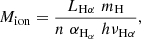
Following Gaspari et al. (2018), Fig. 8 (the kinematical plot, ‘k-plot’) shows the line width of the total [N II]λ6583 line8 versus its velocity centroid (with respect to the systemic velocity of the galaxy) for each independent line of sight detected by MUSE in the innermost arcminute of Fornax A (green colours). Blue dots are the spectra matching the regular rotation. Remarkably, the rotating spectra mark a well-defined region in the k-plot, with average width ∼200 km s−1and the centroids spanning all values, with most points accumulating at ±220 km s−1. The left panel of Fig. 9 shows that the non-rotating points also have clustering patterns: by looking at their density in the k-plot, six different loci can be identified. Their spatial distribution is shown by the same colours in the right panel of the figure. The gas with large line widths (R6, red colours) matches the regions previously identified with highest velocity dispersion well (bottom row of Fig. 5). The spectra with similar widths to the rotating gas but extreme centroids are all in the SE wake of the radio jets (R1, cyan colours) or in the NW bend of the jet (R5, orange colours), suggesting that also this gas may be outflowing (see Sect. 7.2 for further details).
 |
Fig. 8. Velocity dispersion (σlos) versus line shift with respect to the systemic velocity of the [N II]λ6583 emission line (|vlos − vsys|), in logarithmic scale. Pixels matching the modelled rotating disk are shown in blue, while everything else is in green. |
The gas with systematically narrower width than the rotating gas appears mostly distributed along the EW-stripe (R2, R3, and R4, green colours) and in the sub-filaments of the edge-on disk. In Sect. 7.1, we discuss the nature of these filaments according to their kinematical properties.
In Table 2, we show the masses of the ionised gas for each region. The mass of the ionised gas is computed as in, for example, Poggianti et al. (2019):
 (1)
(1)
Masses of the different gaseous features identified in NGC 1316.
where LHα is the luminosity of the Hα line, corrected for dust extinction estimated from the Balmer decrement (e.g., Domínguez et al. 2013). n is the gas density computed from R = [S II]λ6731/[S II]λ6716, following the calibration of Proxauf et al. (2014) (which is valid for 0.4 ≤ R ≤ 1.4). mH is the mass of the hydrogen atom, αHα is the effective Hα recombination coefficient, and hνHα is the energy of the Hα photon.
6.3. The kinematics of the cold gas
We apply the same procedure described in the previous section to study the kinematics of the cold gas. We identify components matching with the regular rotation similarly to the ionised gas. Because of the wide field of view of the cold gas observations, we also include the outer ring in this analysis. In Fig. 10, we identify the same loci that we identified for the ionised gas in the k-plots of the H I (top panel) and CO (bottom panel). The right panels of the figures show their spatial distribution. Compared to the ionised gas, we have fewer independent points because of the coarser spatial resolution of the observations. Most loci correspond to the ones identified in the ionised gas9. The large width and centroid (R1, R5, R6; cyan, orange, and red, respectively) are located in the wake of the radio jets and in the outer rings. The narrow line widths (R2, R3 green colours) of the CO are found perpendicular to the edge-on disk. The H I and CO masses of each region are shown in Table 2. Even though the line widths are intrinsically smaller, similarly to the ionised gas, the rotating H I and CO identify a similar region in the k-plot (with most points around |vlos − vsys|∼224 km s−1, σlos ∼ 80 km s−1). The non-rotating points are also clustering in the region with the high sigma and centroid (σlos ≳ 125 km s−1, |vlos − vsys|∼224 km s−1).
7. Discussion
We relate the kinematical properties of the loci identified in the k-plot of the ionised and cold gas to their impact on the AGN activity.
7.1. Feeding: Raining multi-phase clouds and filaments via turbulent condensation
The k-plots shown in the previous sections indicate that the kinematical properties of the multi-phase gas in Fornax A can be broadly classified in three groups:
-
gas rotating within the inner disk (blue colours, in Figs. 9 and 10)
-
gas distributed in the EW-stripe and filaments perpendicular to the rotating disk with narrow line-widths (R2, R3, and R4; green colours)
-
gas distributed in clouds in the wake of the radio jets and in the outer ring with large line widths (R1 in cyan and R5 and R6 in red colours).
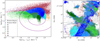 |
Fig. 9. Left panel: velocity dispersion versus line shift (k-plot) with respect to the systemic velocity of the [N II]λ6583 line emission in logarithmic scale. Colours identify different regions in the plot. Pixels consistent with the model of rotation are shown in blue, while pixels in the kinematical region of rotation are shown in light blue. The purple ellipses show the 1, 2σ confidence intervals tied to the global log-normal distributions found for chaotic cold accretions (Gaspari et al. 2018). Right panel: distribution of the ionised gas. Colours correspond to the plot in the left panel. Radio jets are shown by black contours. |
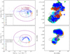 |
Fig. 10. Left panels: velocity dispersion versus line shift with respect to the systemic velocity of the H I and CO, respectively, in logarithmic scale. Colours identify different regions in the plot. Pixels consistent with the model of rotation are shown in blue, while pixels in the kinematical region of rotation are shown in light blue. The purple ellipses are the same as in the left panel of Fig. 9. Right panels: distribution of the H I and CO, respectively. Colours correspond to the plot in the left panel. Radio jets are shown in grey. The H I and CO different loci, in particular R6 and the rotating regions, are distributed similarly to the ionised gas regions, but on a larger scale. |
The physical properties of the cold gas in these regions are also very different (see Sect. 4); that is, the rotating regions have the highest H2/H I ratio, while this ratio decreases in the outflow and is ≲1 in the EW stripe. The EW stripe and filaments have the most peculiar morphological and kinematical properties. The EW stripe has kinematics in conflict with a rotating circumnuclear disk, as indicated by the presence of redshifted velocities with regard to vsys on both sides of the centre. These shifts are small and, along with the small velocity dispersion of the stripe, suggest it is not outflowing. The sub-filaments are spatially connected to the edge-on disk, but their kinematics are very different. They are highly redshifted compared to the overall rotation of the disk, and have narrower line widths.
The k-plot gives us a hint as to the nature of the EW stripe and filaments. The purple ellipses in the left panels of Figs. 9 and 10 show the mean value of line widths and shifts ±1, 2σ that would be expected from CCA simulations if the cold and ionised gas were undergoing condensation and inducing rainfalls (see Fig. 4 of Gaspari et al. 2018). In the ionised and H I gas, the EW stripe and filaments are consistent with the expectations of CCA. The k-plot also shows that the outer edges of the EW stripe (R2) are more compatible with CCA than the inner regions (R3, R4). This is possibly because the core of Fornax A may have been recently re-activated (Maccagni et al. 2020) and the innermost regions are perturbed by its activity (as is suggested by the presence of a broad component, σ ≳ 300 km s−1 in the ionised gas emission lines).
The turbulent Taylor number Tat ≡ vrot/σv,3D (Gaspari et al. 2017)10 is a key dimensionless number that compares the rotating and turbulent kinematics. Typically, when Tat < 3 turbulence becomes significant compared to rotation and chaotic condensation may occur because of it. Particularly below the unity threshold, CCA becomes vigorous and induces extended filamentary condensation instead of a more disk-dominated condensation (Gaspari et al. 2015).
Here, we use the Taylor number to determine the role of turbulence of the multi-phase ISM in the centre of Fornax A. In the EW stripe and filaments, since their kinematics is not compatible with rotation, vrot → 0 and Tat → 0. Even though the gas in the inner disk is dominated by rotation, its velocity dispersion (σlos) is high in all phases of the gas (as discussed in the previous sections). Hence, we compute Tat for all phases throughout the disk. From the rotating model (Sect. 6.1), we fix vrot = 340sin(i) km s−1, while we measure σlos(r) as the mean value in radial bins of 1 kpc. The results are shown in Fig. 11. With dotted lines and labels, we highlight where turbulence becomes significant and starts to perturb the rotating disk.
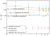 |
Fig. 11. Radial profile of the Taylor number (Tat = vrot/σlos; Gaspari et al. 2015, 2017), in logarithmic scale. In green, orange, and blue, we show three phases of the gas within the rotating disk, in red the upper limits to Tat of the EW-stripe and filaments outside the disk, which are mostly dominated by pure turbulence. We label the areas of rough transition from rotation- to turbulence-dominated (‘CCA-driven’) kinematics, with dotted lines as separators. |
The figure shows that the ionised and (inner) H I gas phases inside the disk are still altered by turbulence. Several clouds in these phases may be interacting with in-falling clouds, which perturbs the coherent rotational structure, hence driving a clumpy disk. The ionised gas always has Tat ∼ 1; that is, the turbulent component mildly dominates over the rotational velocity. Thus, we expect strong clumpyness and/or filaments of this gas (and related boosted CCA feeding), as unveiled by the emission maps (Fig. 5) and k-plot (Fig. 9) in a consistent manner. The molecular component in the disk appears to reside in the pure rotational regime, as it is physically the densest and thus most compact phase, which is difficult to internally perturb via turbulent motions (e.g., Gaspari et al. 2017).
Further constraints on the feeding nature of the EW stripe and filaments can be given by the radial variation of the C-ratio in the different phases of the gas. The C-ratio (C ≡ tcool/teddy) is the criterion closely related to CCA and ensuing top-down condensation cascade (Gaspari et al. 2018). When the eddy turnover timescale (teddy = 2πr1/3L2/3/σv,3D(r)) is comparable to the cooling time, extended filamentary and cloudy condensation can efficiently occur. The cooling time is defined from the properties of the X-ray halo in which the galaxy is embedded, tcool = 3kbT/neΛ (where Λ(T, Z) is the plasma cooling function; Sutherland & Dopita 1993). The C-ratio has already been used to link the level of thermal instability of the ISM, Intra-Group Medium, and ICM to the on-going nuclear activity of different AGNs, such as Abell 2597 (Tremblay et al. 2018), NGC 7409 (Juráňová et al. 2019), and a dozen other clusters (Olivares et al. 2019).
We estimate the cooling time in the centre of Fornax A from the temperature of the X-ray halo measured by Nagino & Matsushita (2009) between 1 and 8 kpc, ⟨Tx⟩ = 0.77 keV. Since the turbulence velocities of the ionised gas linearly correlate (with a scatter of 14%) with the velocities of the X-ray emitting gas (Gaspari et al. 2018), we determine the C-ratio of three different regions of Fornax A from the kinematics of the ionised gas. The regions are selected from the k-plot: the gas that is rotating, the gas likely outflowing (R1, R5, and R6), and the gas with kinematics compatible with the expectations of CCA (the EW stripe and filaments R2, R3, R4). To determine the C-ratio, we measure the mean values of the velocity dispersion in radial bins of 1 kpc along the selected regions.
The results are shown in Fig. 12. The purple band indicates when the gas is being driven by non-linear thermal instabilities (in particular around unity value). The outflowing and rotating regions have C-ratio significantly above unity, hence the multi-phase condensation is weak, if not delayed. Conversely, the CCA regions are those with the lowest C-ratio approaching unity, especially at intermediate and large radial distances. The most thermally unstable region is the EW stripe, which is consistent with the above inspection of the maps and k-plot. This stripe is also perpendicular to the outflow and disk region, as expected in typical self-regulated CCA/feeding and bipolar outflow/feedback cycles (e.g., Gaspari et al. 2012). The mass of the EW stripe is 3.5 × 10⁵ M⊙ for the ionised gas, 4.3 × 10⁶ M⊙ for the H I, and 9.6 × 10⁶ M⊙ for the H2 derived from the CO observations. The latest episodes of nuclear activity of Fornax A were rapid (1–3 Myr; Maccagni et al. 2020) and emitted energies typical of low-excitation radio galaxies (λ = (Lmech + Lrad)/LEdd ∼ 10−3). Under low-efficiency accretion regimes (Ṁ ≲ 0.1 M⊙ yr−1) the mass of the filaments is sufficient to fuel the nuclear activity.
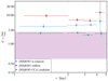 |
Fig. 12. Radial profile of the C-ratio (tcool/teddy) in logarithmic scale. The purple-shaded area shows where the gas becomes thermally unstable, leading to extended filamentary condensation and the CCA rain (e.g., Gaspari et al. 2018). |
The above k-plot, together with the Taylor number and the C-ratio constraints, as well as the rapid flickering in the low-power regime, show that CCA is very likely on-going within the EW stripe. There, gas is likely condensing from a diffuse ionised phase to neutral and then to molecular clouds, thus fuelling the nuclear activity of Fornax A.
Besides its kinematical properties, the EW stripe also has physical differences compared to the gas in the centre and the outer ring. As shown in Fig. 5, the stripe is clearly detected in the low-ionisation lines ([S II]λλ6716,6731, [N II], Hα) but is much weaker in the high-ionisation lines (Hβ, [O III], and [O I]11). Given that the high-ionisation lines are better tracers of shocks and heating processes, this further suggests the condensing nature of the EW stripe compared to the other regions identified in the k-plot, since feeding proceeds more abundantly when heating is low and cooling is high (this is also why feeding seems more pronounced perpendicular to the jet region). The EW stripe is rich in ionised gas and H I but lacks molecular gas (Sect. 4) and dust (Fig. 1). Plausibly, even though accreting, the stripe has not reached the final phase of condensation yet.
7.2. Feedback: Outflowing gas in the wake of the radio jets
The velocity fields and dispersion maps of the cold and ionised gas (Figs. 3 and 5, respectively), as well as the k-plot of the multi-phase ISM (Figs. 9 and 10), show that in the centre and along the radio jets of Fornax A in different regions (R1, R5, and R6 in the k-plots) the gas has extreme line widths and/or is highly shifted with regard to vsys, suggesting the presence of an outflowing component. For a direct comparison with previous works on outflowing gas in AGNs (see, for example, Harrison et al. 2016; Wylezalek et al. 2020; Kakkad et al. 2020) as a measurement of these extreme line widths, we adopt the width at 80% of the total flux of the [N II]λ6583 line, w80. Its distribution is shown in Fig. 13. The colour scale highlights the regions where the w80 ≳ 600 km s−1, which is a typical velocity cut-off used to define gaseous outflows. The figure shows the filamentary nature of the outflows and the close correspondence with the main features of the radio jets: the core, the wake in the innermost kilo-parsec, and the bends at ∼4.5 kpc from the centre.
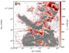 |
Fig. 13. Map of the w80 of the total [N II]λ6583 line. Values above 600 km s−1 may indicate the presence of outflowing gas, and are shown in colour scale. The radio jets are shown by black contours. |
Figure 14 shows that where the ionised gas seems to be outflowing, the cold component also has extreme kinematics (w80 ≳ 200 km s−1)12. Because of the wider field of view of the H I and CO observations, we notice that large line widths are also present in the ring, further suggesting the presence of a multi-phase outflow out to 6 kpc from the AGN. Given that to reach this distance the gas in the outer ring may have taken the same amount of time as the age of the radio jets (3 Myr at vOUT ∼ 2000 km s−1, see Sect. 6), the turbulent kinematics of the outer ring were possibly caused by the same nuclear activity that generated the jets.
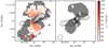 |
Fig. 14. Left panel: map of the w80 of the H I line. Regions with broad emission w80 ≳ 200 km s−1 are coincident with regions where ionised gas may be outflowing. Right panel: map of the w80 of the 12CO(1−0) line. Regions with broad emission w80 ≳ 200 km s−1 are coincident with regions where ionised gas may be outflowing. |
Outflowing gas extending for several kilo-parsecs in AGNs are typically detected in a bi-conical distribution, perpendicularly or along the jets (as in, for example, NGC 1266 and NGC 1068; see Alatalo et al. 2011; García-Burillo et al. 2019, respectively), and present radial velocities of several thousands of km s−1. In Fornax A, instead, we detect a ring-like distribution of the gas with radial velocities not as extreme (∼2000 km s−1). A possible explanation may lie in the history of the nuclear activity of Fornax A. Since the jets are not currently active, but have possibly been adiabatically expanding through the ISM for the last 2 Myr, we are seeing a post-outflowing phase where the kinematics are still turbulent, but the AGN winds are not accelerating nor exciting the gas anymore. This would also explain the LINER-like excitation rates of the outflowing material.
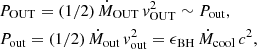
Since the w80 maps are compatible with the results of the k-plot, we use the masses of the H I, CO, and ionised gas in regions R1, R5, and R6 (see Table 2) to determine the total mass of the outflow Mout ∼ 2 × 10⁷ M⊙. Assuming that the outflow was ejected at the same time of the jets, the mass outflow rate is ṀOUT ∼ 5 M⊙ yr−1.
The (macro) outflowing power is 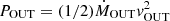 (see, for example, Gaspari 2017). From the kinematics of the multi-phase outer ring, we assume vOUT = 2000 km s−1 and estimate POUT ∼ 6 × 1042 erg s−1. The outflowing power is compatible with the power of the last nuclear activity of Fornax A defined as Lmech, jets + Lrad. The mechanical power of the radio jets (Lmech, jets ∼ 2.4 × 1042 erg s−1) is inferred from their 1.44 GHz luminosity (L1.44 GHz, jets; Cavagnolo et al. 2010), while the radiative power (Lrad ∼ 3.4 × 1042 erg s−1) follows from the total luminosity of the [O III]λ5007 line of the outflow (L[OIII]5007 ≳ 9.8 × 1038 erg s−1) (Heckman et al. 2004).
The outflow power is compatible with the mechanical plus radiated power emitted by Fornax A in the last phase of activity (L = Lmech + Lrad ≳ 6.0 × 1042 erg s−1). This further indicates that the nuclear activity that generated the jets of Fornax A also entrained the gaseous outflow out to distances of ∼6 kpc.
7.3. The self-regulated flickering activity of Fornax A
The radio continuum properties of Fornax A suggest that its nuclear activity is rapidly flickering. In the last ∼3 Myr two different episodes occurred, one that formed the jets and one that may still be ongoing (Maccagni et al. 2020).
In the previous sections, we show that in the innermost 6 kpc of Fornax A, the gas experiencing condensation and turbulently raining co-exists with a regular ring that makes up most of the gas mass and gas outflowing as a consequence of the nuclear activity that occurred ∼3 Myr ago. The properties of both the outflow and the in-flowing gas are consistent with the predictions of the CCA model. Here, we argue that the rapid flickering of Fornax A is also self-regulated via CCA.
Within the framework of CCA, the macro scale properties of the outflow can be linked to the mass that was accreted to fuel the nuclear activity. Feedback outbursts, propagating from the micro scale near the SMBH to the macro scales of the host galaxy/cluster, balance the cooling flow occurring at tens of kpc. Hence, AGN feedback must be significantly ‘energy conserving’ over great distances and long periods, with the power emitted at the micro scale (Pout) roughly comparable to the power of the macro outflow (POUT), and proportional to the luminosity of the X-ray halo. Following Gaspari (2017), the large-scale outflow power is linked to the CCA mass accreted by the SMBH (Ṁcool), such as
 (2)
(2)
where ϵBH = 10−3 (Tx/2.5 keV) is the macro-scale mechanical efficiency, which is tied to the temperature of the X-ray emitting halo (∼0.7 keV). Consequently, the accretion rate (quenched cooling flow) needed to sustain the formation of the jets and generate the outflow is Ṁcool ∼ 0.4 M⊙ yr−1. Assuming the age of the jets (∼3 Myr) as an upper limit to the accretion, the total accreted mass is of the order of 106 M⊙, which is a fraction of the cold gas mass of the EW stripe, as expected. Based on Eq. (2) and outflow scalings of Gaspari (2017), we can also estimate the properties of the micro feedback: vout ≈ 104 km s−1 and Ṁout ≃ 0.2 M⊙ yr−1, which are consistent with the values of micro ultra-fast X-ray outflows (Tombesi et al. 2013). From this, we can assess the entrainment factor η = ṀOUT/Ṁout ∼ 25, which indicates that the primary macro driver is the ionised/neutral component, rather than the molecular phase (with expected η ≫ 100). As shown by the above MUSE and MeerKAT w80 maps, such phases are indeed the main drivers of the outflowing gas.
The k-plot, Taylor number, and C-ratio provide major evidence that the EW stripe is likely experiencing CCA. In these regions, according to CCA modelling, gas becomes thermally unstable in a non-linear way, generating substantial CCA rain unhindered by rotation, which will feed the SMBH via inelastic collisions as the clouds fall within r < 300 pc. Since the EW stripe extends down to the innermost regions of Fornax A (Sect. 7.1) and is still condensing, it is reasonable to think that part of it recently fuelled the AGN. As CCA typically occurs through recursive precipitation episodes of low-mass feeding rather than a single episode of accretion, this could explain the rapid flickering (a few Myr) of Fornax A in the low-efficiency accretion regime (specifically, CCA typically induces pink-noise 1/f frequency power spectra). Overall, the several examples of independent evidence at the macro and micro spatial scales, tied also to different epochs, have allowed us to achieve a full picture of the self-regulated AGN feeding and feedback cycle in Fornax A, with recursive CCA rainfalls and triggered outflows/jets.
8. Summary and future prospects
In this paper, we showed the distribution of the multi-phase ISM (neutral, molecular, and ionised gas) in Fornax A, focusing on the innermost arcminute (r ≲ 6 kpc). We studied the kinematics of the ISM based on spectral observations of the H I from MeerKAT, of the 12CO(1−0) from ALMA and of the optical emission lines (Hβ, [O III]λ4959, [O III]λ5007, [N II]λ6548, Hα, [N II]λ6583, and [S II]λλ6716,6731) from MUSE. We used different methods that allowed us to identify both multi-phase gaseous inflows and outflows that are likely involved in the feeding and feedback processes of the AGN.
In the innermost arcminute, most gas is distributed in a rotating, nearly edge-on disk (r ≲ 4 kpc). At outer radii (4.5 ≲ r ≲ 6.5), the gas is found in a ring at the edge of the radio jets. The detailed analysis of the kinematics of the gas (Sect. 6) suggests that the inner disk is rotating, while the outer ring is outflowing, ejected by the nuclear episode that also formed the jets. The cool phase is the most massive of the outflow (Mout ∼ 2 × 10⁷ M⊙). The macro-outflowing power ( ) is compatible with the power of the last phase of activity of Fornax A. The outflowing gas of the ring and along the jets is the result of the mass entrained by the winds ejected by the AGN.
Besides the outflow, the multi-phase gas kinematics indicate that other components are also non-rotating; that is, some filaments within the inner disk and the EW stripe. The kinematical-plot (Sect. 6.2) for the multi-phase gas (introduced by Gaspari et al. 2018) is a powerful method to identify all-at-once gaseous components that deviate from regular rotation. This allowed us to identify that the EW stripe and filaments have narrow line widths and line shifts typical of gas undergoing CCA (Sect. 7.1), and they may be feeding the AGN. The C-ratio (Fig. 12) indicates that in these regions the eddy-turnover timescale is roughly comparable to the cooling time and that condensation may efficiently occur, driving the gas to rain towards the centre and fuel the AGN. The mass of the in-falling filaments (dominated by the cold gas) is sufficient to feed the low-efficiency accretion regime of the current activity.
In Fornax A, events of feeding and feedback are detected in the multi-phase gas over different scales (from ≲1 kpc to ∼6 kpc) and appear to co-exist in space and time, showing clear indications of preceding/ongoing and forthcoming condensation events. The connection between the properties of the macro-scale outflow and the in-falling gas suggests that the rapid flickering of the nuclear activity (1–3 Myr) is self-regulated by recurring CCA (Gaspari et al. 2017). Deeper X-ray observations may provide further information on this cycle by detecting the blueshifted absorption lines related to the micro AGN outflows.
The kinematical analysis of the multi-phase ISM in Fornax A reveals both feeding and feedback events and provides several quantitative evidences that CCA may be regulating its recurrent activity – making it arguably one of the most in-depth studies probing this mechanism. A complete study of the physical properties of the multi-phase gas, for example through the analysis of the ionised gas emission line ratios and by the high resolution observations of multiple transitions of the CO, may allow us to gain further insights on the role of turbulence (and CCA) in sustaining the rapid AGN flickering and the effects of the outflow on the evolution of radio AGNs.
 .
.
Since the total line is made of multiple components, we compute the line-width as the dispersion of the total fitted line.
Except for R4, which has too few points and is included in R3.
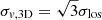 is the three-dimensional velocity dispersion.
Not shown in the figure.
In the MeerKAT and ALMA observations, the shallow broad wings that dominate w80 are often seen below the S/N ∼ 3, making a direct measurement of the full extent of the lines uncertain. Hence, we infer w80 from the dispersion of the line assuming the relation for a single Gaussian profile (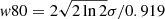 ).
).
Acknowledgments
The authors thank the anonymous referee for the useful comments and suggestions. This project has received funding from the European Research Council (ERC) under the European Union’s Horizon 2020 research and innovation programme (grant agreement no. 679627). We are grateful to the full MeerKAT team at SARAO for their work on building and commissioning MeerKAT. The MeerKAT telescope is operated by the South African Radio Astronomy Observatory, which is a facility of the National Research Foundation, an agency of the Department of Science and Innovation. This paper makes use of the following ALMA data: ADS/JAO.ALMA#2017.1.00129.S. ALMA is a partnership of ESO (representing its member states). NSF (USA) and NINS (Japan), together with NRC (Canada), MOST and ASAIA (Taiwan), and KASI (Republic of Korea), in cooperation with the Republic of Chile. The Joint ALMA Observatory is operated by ESO, AUI/NRAO and NAOJ. The VLA images at 4.8 and 14.4 GHz have been produced as part of the NRAO VLA Archive Survey, (c) AUI/NRAO. The National Radio Astronomy Observatory (NRAO) is a facility of the National Science Foundation, operated under cooperative agreement by Associated Universities, Inc. This research made use of Montage. It is funded by the National Science Foundation under Grant Number ACI-1440620, and was previously funded by the National Aeronautics and Space Administration’s Earth Science Technology Office, Computation Technologies Project, under Cooperative Agreement Number NCC5-626 between NASA and the California Institute of Technology. This research was supported by the Munich Institute for Astro- and Particle Physics (MIAPP) of the DFG cluster of excellence ‘Origin and Structure of the Universe’. M.G. acknowledges partial support by NASA Chandra GO8-19104X/GO9-20114X and HST GO-15890.020-A grants. K.M. acknowledges JSPS KAKENHI Grant Numbers of 19J40004 and 19H01931. O.S.’ research is supported by the South African Research Chairs Initiative of the Department of Science and Technology and National Research Foundation.
References
- Alatalo, K., Blitz, L., Young, L. M., et al. 2011, ApJ, 735, 88 [NASA ADS] [CrossRef] [Google Scholar]
- Audibert, A., Combes, F., García-Burillo, S., et al. 2021, A&A, in press, https://doi.org/10.1051/0004-6361/202039886 [NASA ADS] [CrossRef] [EDP Sciences] [Google Scholar]
- Baldi, R. D., Rodríguez Zaurín, J., Chiaberge, M., et al. 2019, ApJ, 870, 53 [CrossRef] [Google Scholar]
- Bittner, A., Falcón-Barroso, J., Nedelchev, B., et al. 2019, A&A, 628, A117 [NASA ADS] [CrossRef] [EDP Sciences] [Google Scholar]
- Bolatto, A. D., Wolfire, M., & Leroy, A. K. 2013, ARA&A, 51, 207 [CrossRef] [Google Scholar]
- Brienza, M., Godfrey, L., Morganti, R., et al. 2017, A&A, 606, A98 [NASA ADS] [CrossRef] [EDP Sciences] [Google Scholar]
- Brocksopp, C., Kaiser, C. R., Schoenmakers, A. P., & de Bruyn, A. G. 2007, MNRAS, 382, 1019 [NASA ADS] [CrossRef] [Google Scholar]
- Camilo, F., Scholz, P., Serylak, M., et al. 2018, ApJ, 856, 180 [Google Scholar]
- Cano-Díaz, M., Maiolino, R., Marconi, A., et al. 2012, A&A, 537, L8 [NASA ADS] [CrossRef] [EDP Sciences] [Google Scholar]
- Cantiello, M., Grado, A., Blakeslee, J. P., et al. 2013, A&A, 552, A106 [NASA ADS] [CrossRef] [EDP Sciences] [Google Scholar]
- Cappellari, M. 2017, MNRAS, 466, 798 [Google Scholar]
- Cappellari, M., & Emsellem, E. 2004, PASP, 116, 138 [Google Scholar]
- Carniani, S., Marconi, A., Maiolino, R., et al. 2016, A&A, 591, A28 [NASA ADS] [CrossRef] [EDP Sciences] [Google Scholar]
- Cavagnolo, K. W., McNamara, B. R., Nulsen, P. E. J., et al. 2010, ApJ, 720, 1066 [Google Scholar]
- Churazov, E., Vikhlinin, A., Zhuravleva, I., et al. 2012, MNRAS, 421, 1123 [NASA ADS] [CrossRef] [Google Scholar]
- Cicone, C., Brusa, M., Ramos Almeida, C., et al. 2018, Nat. Astron., 2, 176 [Google Scholar]
- Ciotti, L., Ostriker, J. P., & Proga, D. 2010, ApJ, 717, 708 [Google Scholar]
- Combes, F., García-Burillo, S., Casasola, V., et al. 2013, A&A, 558, A124 [NASA ADS] [CrossRef] [EDP Sciences] [Google Scholar]
- Cordey, R. A. 1987, MNRAS, 227, 695 [NASA ADS] [Google Scholar]
- Davies, R., Baron, D., Shimizu, T., et al. 2020, MNRAS, 498, 4150 [Google Scholar]
- de Blok, W. J. G., Athanassoula, E., Bosma, A., et al. 2020, A&A, 643, A147 [NASA ADS] [CrossRef] [EDP Sciences] [Google Scholar]
- den Heijer, M., Oosterloo, T. A., Serra, P., et al. 2015, A&A, 581, A98 [NASA ADS] [CrossRef] [EDP Sciences] [Google Scholar]
- Di Teodoro, E. M., & Fraternali, F. 2015, MNRAS, 451, 3021 [Google Scholar]
- Domínguez, A., Siana, B., Henry, A. L., et al. 2013, ApJ, 763, 145 [CrossRef] [Google Scholar]
- Duah Asabere, B., Horellou, C., Jarrett, T. H., & Winkler, H. 2016, A&A, 592, A20 [NASA ADS] [CrossRef] [EDP Sciences] [Google Scholar]
- Fabian, A. C. 2012, ARA&A, 50, 455 [Google Scholar]
- Fluetsch, A., Maiolino, R., Carniani, S., et al. 2021, MNRAS, 505, 5753 [NASA ADS] [CrossRef] [Google Scholar]
- Galametz, M., Kennicutt, R. C., Albrecht, M., et al. 2012, MNRAS, 425, 763 [NASA ADS] [CrossRef] [Google Scholar]
- Galametz, M., Albrecht, M., Kennicutt, R., et al. 2014, MNRAS, 439, 2542 [NASA ADS] [CrossRef] [Google Scholar]
- García-Burillo, S., Combes, F., Ramos Almeida, C., et al. 2019, A&A, 632, A61 [Google Scholar]
- Gaspari, M., & Sądowski, A. 2017, ApJ, 837, 149 [NASA ADS] [CrossRef] [Google Scholar]
- Gaspari, M., Brighenti, F., & Temi, P. 2012, MNRAS, 424, 190 [NASA ADS] [CrossRef] [Google Scholar]
- Gaspari, M., Ruszkowski, M., & Oh, S. P. 2013, MNRAS, 432, 3401 [NASA ADS] [CrossRef] [Google Scholar]
- Gaspari, M., Brighenti, F., & Temi, P. 2015, A&A, 579, A62 [NASA ADS] [CrossRef] [EDP Sciences] [Google Scholar]
- Gaspari, M., Temi, P., & Brighenti, F. 2017, MNRAS, 466, 677 [Google Scholar]
- Gaspari, M., McDonald, M., Hamer, S. L., et al. 2018, ApJ, 854, 167 [Google Scholar]
- Gaspari, M., Eckert, D., Ettori, S., et al. 2019, ApJ, 884, 169 [NASA ADS] [CrossRef] [Google Scholar]
- Gaspari, M., Tombesi, F., & Cappi, M. 2020, Nat. Astron., 4, 10 [Google Scholar]
- Harrison, C. M. 2017, Nat. Astron., 1, 0165 [NASA ADS] [CrossRef] [Google Scholar]
- Harrison, C. M., Alexander, D. M., Mullaney, J. R., et al. 2016, MNRAS, 456, 1195 [Google Scholar]
- Heckman, T. M., Kauffmann, G., Brinchmann, J., et al. 2004, ApJ, 613, 109 [Google Scholar]
- Horellou, C., Black, J. H., van Gorkom, J. H., et al. 2001, A&A, 376, 837 [NASA ADS] [CrossRef] [EDP Sciences] [Google Scholar]
- Iodice, E., Spavone, M., Capaccioli, M., et al. 2017, ApJ, 839, 21 [Google Scholar]
- Jonas, J., & MeerKAT Team 2016, in MeerKAT Science: On the Pathway to the SKA, 1 [Google Scholar]
- Józsa, G. I. G., White, S. V., Thorat, K., et al. 2020, CARACal: Containerized Automated Radio Astronomy Calibration pipeline [Google Scholar]
- Juráňová, A., Werner, N., Gaspari, M., et al. 2019, MNRAS, 484, 2886 [CrossRef] [Google Scholar]
- Juráňová, A., Werner, N., Nulsen, P. E. J., et al. 2020, MNRAS, 499, 5163 [CrossRef] [Google Scholar]
- Kakkad, D., Mainieri, V., Vietri, G., et al. 2020, A&A, 642, A147 [NASA ADS] [CrossRef] [EDP Sciences] [Google Scholar]
- King, A., & Nixon, C. 2015, MNRAS, 453, L46 [NASA ADS] [CrossRef] [Google Scholar]
- King, A., & Pounds, K. 2015, ARA&A, 53, 115 [NASA ADS] [CrossRef] [Google Scholar]
- Kleiner, D., Serra, P., Maccagni, F. M., et al. 2021, A&A, 648, A32 [NASA ADS] [CrossRef] [EDP Sciences] [Google Scholar]
- Krajnović, D., Weilbacher, P. M., Urrutia, T., et al. 2015, MNRAS, 452, 2 [Google Scholar]
- Lakhchaura, K., Werner, N., Sun, M., et al. 2018, MNRAS, 481, 4472 [NASA ADS] [CrossRef] [Google Scholar]
- Lanz, L., Jones, C., Forman, W. R., et al. 2010, ApJ, 721, 1702 [NASA ADS] [CrossRef] [Google Scholar]
- López-Cobá, C., Sánchez, S. F., Anderson, J. P., et al. 2020, AJ, 159, 167 [Google Scholar]
- Maccagni, F. M., Morganti, R., Oosterloo, T. A., & Mahony, E. K. 2014, A&A, 571, A67 [NASA ADS] [CrossRef] [EDP Sciences] [Google Scholar]
- Maccagni, F. M., Santoro, F., Morganti, R., et al. 2016, A&A, 588, A46 [NASA ADS] [CrossRef] [EDP Sciences] [Google Scholar]
- Maccagni, F. M., Morganti, R., Oosterloo, T. A., Oonk, J. B. R., & Emonts, B. H. C. 2018, A&A, 614, A42 [NASA ADS] [CrossRef] [EDP Sciences] [Google Scholar]
- Maccagni, F. M., Murgia, M., Serra, P., et al. 2020, A&A, 634, A9 [NASA ADS] [CrossRef] [EDP Sciences] [Google Scholar]
- Mackie, G., & Fabbiano, G. 1998, AJ, 115, 514 [NASA ADS] [CrossRef] [Google Scholar]
- McDonald, M., Gaspari, M., McNamara, B. R., & Tremblay, G. R. 2018, ApJ, 858, 45 [Google Scholar]
- McNamara, B. R., & Nulsen, P. E. J. 2012, New J. Phys., 14, 055023 [NASA ADS] [CrossRef] [Google Scholar]
- Meyer, M., Robotham, A., Obreschkow, D., et al. 2017, PASA, 34, 52 [Google Scholar]
- Michałowski, M. J., Kamphuis, P., Hjorth, J., et al. 2019, A&A, 627, A106 [NASA ADS] [CrossRef] [EDP Sciences] [Google Scholar]
- Mingozzi, M., Cresci, G., Venturi, G., et al. 2019, A&A, 622, A146 [NASA ADS] [CrossRef] [EDP Sciences] [Google Scholar]
- Morganti, R., & Oosterloo, T. 2018, A&ARv, 26, 4 [Google Scholar]
- Morganti, R., Oosterloo, T. A., Brienza, M., et al. 2021, A&A, 648, A9 [EDP Sciences] [Google Scholar]
- Morokuma-Matsui, K., Serra, P., Maccagni, F. M., et al. 2019, PASJ, 71, 85 [NASA ADS] [CrossRef] [Google Scholar]
- Nagino, R., & Matsushita, K. 2009, A&A, 501, 157 [NASA ADS] [CrossRef] [EDP Sciences] [Google Scholar]
- Newville, M., Stensitzki, T., Allen, D. B., & Ingargiola, A. 2014, LMFIT: Non-Linear Least-Square Minimization and Curve-Fitting for Python [Google Scholar]
- Noordermeer, E., van der Hulst, J. M., Sancisi, R., Swaters, R. S., & van Albada, T. S. 2007, MNRAS, 376, 1513 [NASA ADS] [CrossRef] [Google Scholar]
- Olivares, V., Salome, P., Combes, F., et al. 2019, A&A, 631, A22 [NASA ADS] [CrossRef] [EDP Sciences] [Google Scholar]
- Oosterloo, T., Morganti, R., Tadhunter, C., et al. 2019, A&A, 632, A66 [NASA ADS] [CrossRef] [EDP Sciences] [Google Scholar]
- Orrù, E., van Velzen, S., Pizzo, R. F., et al. 2015, A&A, 584, A112 [NASA ADS] [CrossRef] [EDP Sciences] [Google Scholar]
- Poggianti, B. M., Gullieuszik, M., Tonnesen, S., et al. 2019, MNRAS, 482, 4466 [Google Scholar]
- Prasad, D., Sharma, P., & Babul, A. 2017, MNRAS, 471, 1531 [NASA ADS] [CrossRef] [Google Scholar]
- Prieto, J., Escala, A., Privon, G., & d’Etigny, J. 2021, MNRAS, 508, 3672 [NASA ADS] [CrossRef] [Google Scholar]
- Proxauf, B., Öttl, S., & Kimeswenger, S. 2014, A&A, 561, A10 [NASA ADS] [CrossRef] [EDP Sciences] [Google Scholar]
- Ramatsoku, M., Murgia, M., Vacca, V., et al. 2020a, A&A, 636, L1 [NASA ADS] [CrossRef] [EDP Sciences] [Google Scholar]
- Ramatsoku, M., Serra, P., Poggianti, B. M., et al. 2020b, A&A, 640, A22 [NASA ADS] [CrossRef] [EDP Sciences] [Google Scholar]
- Richtler, T., Hilker, M., & Iodice, E. 2020, A&A, 643, A120 [NASA ADS] [CrossRef] [EDP Sciences] [Google Scholar]
- Roberts-Borsani, G. W., & Saintonge, A. 2019, MNRAS, 482, 4111 [NASA ADS] [Google Scholar]
- Rose, T., Edge, A. C., Combes, F., et al. 2019, MNRAS, 489, 349 [NASA ADS] [CrossRef] [Google Scholar]
- Sabater, J., Best, P. N., Hardcastle, M. J., et al. 2019, A&A, 622, A17 [NASA ADS] [CrossRef] [EDP Sciences] [Google Scholar]
- Sage, L. J., & Galletta, G. 1993, ApJ, 419, 544 [NASA ADS] [CrossRef] [Google Scholar]
- Saikia, D. J., & Jamrozy, M. 2009, Bull. Astron. Soc. India, 37, 63 [NASA ADS] [Google Scholar]
- Sánchez-Blázquez, P., Gorgas, J., Cardiel, N., & González, J. J. 2006, A&A, 457, 787 [CrossRef] [EDP Sciences] [Google Scholar]
- Schweizer, F. 1980, ApJ, 237, 303 [Google Scholar]
- Serra, P., Westmeier, T., Giese, N., et al. 2015, MNRAS, 448, 1922 [Google Scholar]
- Serra, P., Maccagni, F. M., Kleiner, D., et al. 2019, A&A, 628, A122 [NASA ADS] [CrossRef] [EDP Sciences] [Google Scholar]
- Shulevski, A., Morganti, R., Harwood, J. J., et al. 2017, A&A, 600, A65 [NASA ADS] [CrossRef] [EDP Sciences] [Google Scholar]
- Storchi-Bergmann, T., & Schnorr-Müller, A. 2019, Nat. Astron., 3, 48 [Google Scholar]
- Sutherland, R. S., & Dopita, M. A. 1993, ApJS, 88, 253 [Google Scholar]
- Temi, P., Amblard, A., Gitti, M., et al. 2018, ApJ, 858, 17 [NASA ADS] [CrossRef] [Google Scholar]
- Tombesi, F., Cappi, M., Reeves, J. N., et al. 2013, MNRAS, 430, 1102 [Google Scholar]
- Tremblay, G. R., Oonk, J. B. R., Combes, F., et al. 2016, Nature, 534, 218 [NASA ADS] [CrossRef] [Google Scholar]
- Tremblay, G. R., Combes, F., Oonk, J. B. R., et al. 2018, ApJ, 865, 13 [NASA ADS] [CrossRef] [Google Scholar]
- Veilleux, S., Meléndez, M., Tripp, T. M., Hamann, F., & Rupke, D. S. N. 2016, ApJ, 825, 42 [NASA ADS] [CrossRef] [Google Scholar]
- Veilleux, S., Maiolino, R., Bolatto, A. D., & Aalto, S. 2020, A&ARv, 28, 2 [NASA ADS] [CrossRef] [Google Scholar]
- Weilbacher, P. M., Streicher, O., Urrutia, T., et al. 2014, in Astronomical Data Analysis Software and Systems XXIII, eds. N. Manset, & P. Forshay, ASP Conf. Ser., 485, 451 [Google Scholar]
- Wiklind, T., & Henkel, C. 1989, A&A, 225, 1 [NASA ADS] [Google Scholar]
- Wylezalek, D., Flores, A. M., Zakamska, N. L., Greene, J. E., & Riffel, R. A. 2020, MNRAS, 492, 4680 [NASA ADS] [CrossRef] [Google Scholar]
- Yang, H.-Y. K., Gaspari, M., & Marlow, C. 2019, ApJ, 871, 6 [CrossRef] [Google Scholar]
Appendix A: Optical spectra and best fits of the emission lines of ionised gas
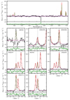 |
Fig. A.1. Centre of Fornax A. |
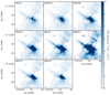 |
Fig. A.5. Total flux density distribution of the fitted lines, on the same colour scale. In all lines, the filamentary structure of the NS disk and EW stripe can be appreciated. The highest emission is found in the centre and along the EW streams. The PSF of the MUSE observations (2″) is shown in the bottom left corner of each panel. Near the SE corner, the gaseous supernova remnant studied by López-Cobá et al. (2020) is visible in the in some ionised lines. The study of this, and other SNe remnants was the main science goal of the centre-field MUSE observations. |
Appendix B: Kinematical model of the ionised gas kinematics
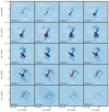 |
Fig. B.1. Consecutive channel maps extracted from the MUSE wide-field datacube. Overlaid in red are the contours of the tilted ring model that best reproduces the [N II]λ6583 emission (as well as the CO and H I seen at lower resolution). We refer the reader to Sect. 6.1 for further details. |
All Tables
All Figures
|
Fig. 1. Hubble ACS visible emission (535 nm) of the centre of Fornax A, radio jets seen by MeerKAT at 1.4 GHz are overlaid in black. Contour levels are 5 × 10−4 × 2n Jy beam−1 (n = 0, 1, 2, …) (Maccagni et al. 2020). |
| In the text | |
|
Fig. 2. Left panel: surface brightness map of the H I gas in the centre of Fornax A. Right panel: same maps for the 12CO(1−0). The PSF of all maps is at 22″ × 18″. Surface brightness contour levels are 3σ × 2n M⊙ pc−2 (n = 0, 1, 2, …) in all panels. The lowest contour corresponds to the 3σ surface brightness detection limit. Radio jets are the same as in Fig. 1. |
| In the text | |
|
Fig. 3. Left panels: velocity and velocity dispersion fields of the H I gas in the centre of Fornax A. Right panels: same maps for the 12CO(1−0). The PSF of all maps is 22″ × 18″. Surface brightness contour levels and radio jets are the same as in Fig. 2. |
| In the text | |
|
Fig. 4. Hubble ACS visible emission (535 nm) of the centre of Fornax A. Green solid contours show regions where the inferred H2 mass surface density is greater than the H I mass surface density (H2/H I ≳ 1), while orange dashed contours show regions rich in atomic hydrogen H I, but where H2 is not detected. The radio jets are shown in black. |
| In the text | |
|
Fig. 5. Flux density distribution (top row), velocity field (central row), and velocity dispersion maps (bottom row) of the ionised gas. Left, middle, and right columns: distribution of the narrow Gaussian component, of the broad Gaussian component, and of the integrated fitted line (narrow+broad components), respectively. The radio jets of Fornax A are overlaid in grey in all panels. See Sect. 5 for details on the regions identified in the top left panel. |
| In the text | |
|
Fig. 6. Position-velocity diagrams along the major axis of the inner nearly edge-on disk. Left panel: Pv-diagram of the atomic and molecular gas (green contours). H I emission is shown by the colour scale and orange solid contours, while absorption is represented by dashed contours. Contour levels are −5; −3; 3, 5, 6, 12, 24σ. Right panel: Pv-diagram derived from the [N II]λ6583 emission (blue colour scale) overlaid with the H I emission and absorption. |
| In the text | |
|
Fig. 7. Consecutive channel maps of the [N II]λ6583 line extracted from the MUSE wide-field datacube in the velocity range 1174 − 2400 km s−1 (the systemic velocity of Fornax A is 1720 km s−1). The contours of the CO emission (0.03, 0.06, 0.12, 0.15, 0.2 Jy beam−1) and of the H I gas (0.15, 0.3, 0.6, 1.2 mJy beam−1) are shown in green and orange, respectively. |
| In the text | |
|
Fig. 8. Velocity dispersion (σlos) versus line shift with respect to the systemic velocity of the [N II]λ6583 emission line (|vlos − vsys|), in logarithmic scale. Pixels matching the modelled rotating disk are shown in blue, while everything else is in green. |
| In the text | |
|
Fig. 9. Left panel: velocity dispersion versus line shift (k-plot) with respect to the systemic velocity of the [N II]λ6583 line emission in logarithmic scale. Colours identify different regions in the plot. Pixels consistent with the model of rotation are shown in blue, while pixels in the kinematical region of rotation are shown in light blue. The purple ellipses show the 1, 2σ confidence intervals tied to the global log-normal distributions found for chaotic cold accretions (Gaspari et al. 2018). Right panel: distribution of the ionised gas. Colours correspond to the plot in the left panel. Radio jets are shown by black contours. |
| In the text | |
|
Fig. 10. Left panels: velocity dispersion versus line shift with respect to the systemic velocity of the H I and CO, respectively, in logarithmic scale. Colours identify different regions in the plot. Pixels consistent with the model of rotation are shown in blue, while pixels in the kinematical region of rotation are shown in light blue. The purple ellipses are the same as in the left panel of Fig. 9. Right panels: distribution of the H I and CO, respectively. Colours correspond to the plot in the left panel. Radio jets are shown in grey. The H I and CO different loci, in particular R6 and the rotating regions, are distributed similarly to the ionised gas regions, but on a larger scale. |
| In the text | |
|
Fig. 11. Radial profile of the Taylor number (Tat = vrot/σlos; Gaspari et al. 2015, 2017), in logarithmic scale. In green, orange, and blue, we show three phases of the gas within the rotating disk, in red the upper limits to Tat of the EW-stripe and filaments outside the disk, which are mostly dominated by pure turbulence. We label the areas of rough transition from rotation- to turbulence-dominated (‘CCA-driven’) kinematics, with dotted lines as separators. |
| In the text | |
|
Fig. 12. Radial profile of the C-ratio (tcool/teddy) in logarithmic scale. The purple-shaded area shows where the gas becomes thermally unstable, leading to extended filamentary condensation and the CCA rain (e.g., Gaspari et al. 2018). |
| In the text | |
|
Fig. 13. Map of the w80 of the total [N II]λ6583 line. Values above 600 km s−1 may indicate the presence of outflowing gas, and are shown in colour scale. The radio jets are shown by black contours. |
| In the text | |
|
Fig. 14. Left panel: map of the w80 of the H I line. Regions with broad emission w80 ≳ 200 km s−1 are coincident with regions where ionised gas may be outflowing. Right panel: map of the w80 of the 12CO(1−0) line. Regions with broad emission w80 ≳ 200 km s−1 are coincident with regions where ionised gas may be outflowing. |
| In the text | |
|
Fig. A.1. Centre of Fornax A. |
| In the text | |
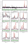 |
Fig. A.2. Region with second Gaussian component along line A in the top left panel of Fig. 5. |
| In the text | |
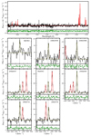 |
Fig. A.3. Stripe; along the east of line B in the top left panel of Fig. 5. |
| In the text | |
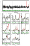 |
Fig. A.4. Cloud; region C in the top left panel of Fig. 5. |
| In the text | |
|
Fig. A.5. Total flux density distribution of the fitted lines, on the same colour scale. In all lines, the filamentary structure of the NS disk and EW stripe can be appreciated. The highest emission is found in the centre and along the EW streams. The PSF of the MUSE observations (2″) is shown in the bottom left corner of each panel. Near the SE corner, the gaseous supernova remnant studied by López-Cobá et al. (2020) is visible in the in some ionised lines. The study of this, and other SNe remnants was the main science goal of the centre-field MUSE observations. |
| In the text | |
|
Fig. B.1. Consecutive channel maps extracted from the MUSE wide-field datacube. Overlaid in red are the contours of the tilted ring model that best reproduces the [N II]λ6583 emission (as well as the CO and H I seen at lower resolution). We refer the reader to Sect. 6.1 for further details. |
| In the text | |
Current usage metrics show cumulative count of Article Views (full-text article views including HTML views, PDF and ePub downloads, according to the available data) and Abstracts Views on Vision4Press platform.
Data correspond to usage on the plateform after 2015. The current usage metrics is available 48-96 hours after online publication and is updated daily on week days.
Initial download of the metrics may take a while.