| Issue |
A&A
Volume 653, September 2021
|
|
|---|---|---|
| Article Number | A94 | |
| Number of page(s) | 28 | |
| Section | The Sun and the Heliosphere | |
| DOI | https://doi.org/10.1051/0004-6361/202140976 | |
| Published online | 15 September 2021 | |
Spectro-imagery of an active tornado-like prominence: Formation and evolution⋆
1
PMOD/WRC, Dorfstrasse 33, 7260 Davos Dorf, Switzerland
e-mail: This email address is being protected from spambots. You need JavaScript enabled to view it.
2
ETH-Zurich, Hönggerberg campus, HIT building, Zürich, Switzerland
3
LESIA, Observatoire de Paris, Université PSL, CNRS, Sorbonne Université, Université Paris-Diderot, 5 place Jules Janssen, 92190 Meudon, France
4
SUPA, School of Physics and Astronomy, University of Glasgow, Scotland, UK
5
KU Leuven, Leuven, Belgium
Received:
1
April
2021
Accepted:
31
May
2021
Abstract
Context. The dynamical nature of fine structures in prominences remains an open issue, including rotating flows in tornado prominences. While the Atmospheric Imaging Assembly imager aboard the Solar Dynamics Observatory allowed us to follow the global structure of a tornado-like prominence for five hours, the Interface Region Imaging Spectrograph, and the Multichannel Subtractive Double Pass spectrograph permitted to obtain plasma diagnostics of its fine structures.
Aims. We aim to address two questions. Firstly, is the observed plasma rotation conceptually acceptable in a flux rope magnetic support configuration with dips? Secondly, how is the plasma density distributed in the tornado-like prominence?
Methods. We calculated line-of-sight velocities and non-thermal line widths using Gaussian fitting for Mg II lines and the bisector method for Hα line. We determined the electron density from Mg II line integrated intensities and profile fitting methods using 1D non-LTE radiative transfer theory models.
Results. The global structure of the prominence observed in Hα, and Mg II h, and k line fits with a magnetic field structure configuration with dips. Coherent Doppler shifts in redshifted and blueshifted areas observed in both lines were detected along rapidly-changing vertical and horizontal structures. However, the tornado at the top of the prominence consists of multiple fine threads with opposite flows, suggesting counter-streaming flows rather than rotation. Surprisingly we found that the electron density at the top of the prominence could be larger (1011 cm−3) than in the inner part of the prominence.
Conclusions. We suggest that the tornado is in a formation state with cooling of hot plasma in a first phase, and following that, a phase of leakage of the formed blobs with large transverse flows of material along long loops extended away from the UV prominence top. The existence of such long magnetic field lines on both sides of the prominence would stop the tornado-like prominence from really turning around its axis.
Key words: Sun: filaments / prominences / Sun: chromosphere / Sun: corona / Sun: UV radiation / techniques: spectroscopic
Movies are available at https://www.aanda.org
© ESO 2021
1. Introduction
Solar prominences are dense and cool plasma structures (104 K) embedded in the hot solar corona (106 K). In chromospheric lines such as Hα, prominences observed on the solar disc appear as darker structures than the surrounding: these structures are called filaments. They lie over magnetic-polarity inversion lines of the radial component of the photospheric magnetic field (see Mackay et al. 2010 for a review). It is accepted that prominence plasma is supported in dips of magnetic field lines either forming an arcade or a flux rope where pressure tension balances the gravitational force (Aulanier & Démoulin 1998; van Ballegooijen 2004; Dudík et al. 2008). Multi-wavelength analysis and magnetic field extrapolations provide us with a large-scale magnetic field topology of solar prominences (Mackay et al. 2010).
The formation of prominences is still an open issue. Different mechanisms suggested by observations or theory have been proposed such as levitation (Okamoto et al. 2010), injection (Magara 2007), or condensation (Mackay et al. 2010). The mechanism of prominence formation by condensation of plasma in the dips of the magnetic field has been well developed since the paper of Karpen et al. (2001), which showed that heating the plasma at the feet of loops generates condensation at the top. Many models and numerical simulations are able to reproduce fine structures of prominences by using this mechanism in 1D models and also in 3D models. The results of these simulations mimic the observations of the Atmospheric Imaging Assembly (AIA) aboard the Solar Dynamics Observatory (SDO) (Karpen et al. 2001; Luna et al. 2012; Xia et al. 2014). Another approach to prove the existence of dips was proposed by Gunár & Mackay (2015, 2016), and Gunár et al. (2018). Their technique attempts to recreate a 3D visualisation of Hα observations. It starts from a 3D magnetic model, provided by simulation or extrapolation, and adds the exchange of emission between the threads using radiative transfer. Their results consisted of the prominence as viewed from different angles, allowing them to directly retrieve all the possible shapes of the simulated prominence from any angle.
However, all of these models are based on the existence of dips. On the other hand, Claes et al. (2020) focussed on hydrodynamics, creating mini thread-like features through non-linear thermal instability that do not strictly outline magnetic field structures. This instability creates blobs, which, after the phase of formation, follow magnetic field lines. This could explain the fragmentation of threads in prominences and high microturbuelence found in active prominence. In some aspects, this can be taken into account for interpreting prominence plasma during the stage of formation.
The determination of plasma properties is an essential component for our understanding of solar prominences, and provides important constraints on the scenarios attempting to explain their characteristics and appearance (see Labrosse et al. 2010 for a review). Chromospheric lines such as hydrogen and Mg II h&k lines give good diagnostics of prominence plasma.
Prominences have long been observed in Hα emission. Hα is an optically thin line and provides information through the prominence along the line of sight (Wiik et al. 1992). Radiative transfer codes were developed in the 90s and provide different characteristics of the hydrogen lines (Lyman, Balmer, and Paschen lines – see Gouttebroze et al. 1993) that can be directly compared with observations (Schmieder et al. 1991, 1999). More recently, a new series of models in 2D configurations were used to interpret the dynamics of multiple threads observed in hydrogen lines (Gunár et al. 2007, 2008).
With the launch of the Interface Region Imaging Spectrograph (IRIS; De Pontieu et al. 2014) in 2013, observations of Mg II lines are now at our disposal. The resonance lines of Mg II, h (2803.5 Å), and k (2796.4 Å) present self-reversed profiles on the solar disc. Their emission along the line profile represents the physical conditions of the plasma at different temperatures in the solar atmosphere. For example, along Mg II k, the k1 minimum is formed in the lower chromosphere, the k2 peaks are formed in the middle chromosphere, and the k3 self-reversal in the upper chromosphere (Leenaarts et al. 2013a,b). Nevertheless, in prominences, Mg II h and k often exhibit single peaked line profiles (Levens et al. 2016; Ruan et al. 2018). This allows us to fit the profiles with a Gaussian profile. However, in other observed prominences, wide Mg II profiles showing two peaks have been interpreted as multiple components corresponding to multiple structures crossing the line of sight (LOS), and they are different to self-reversal lines observed at the solar disc (Schmieder et al. 2014; Ruan et al. 2018).
The radiative transfer behind the formation of these Mg II profiles has recently been studied by Heinzel et al. (2014, 2015); Jejčič et al. (2018), and Levens & Labrosse (2019). Electron density and optical thickness were deduced from observations of the full width at half maximum (FWHM), integrated intensities of Hα and Mg II in prominences (Ruan et al. 2018). The core of Mg II is optically thick and the emission comes from the surface layers of prominences, while the wings are optically thinner and the emission here encapsulates that of all of the structures along the LOS. Therefore, Doppler shifts measured in the Mg II wings could be similar to those calculated in Hα, as shown by Ruan et al. (2018).
Details of IRIS, MSDP, and SDO/AIA observations made on 19 April 2018.
Properties of observed spectral lines.
Characteristics of Mg II k and h line profiles of IRIS raster 8 (slit 12 at 16:34:10 UT and slit 23 at 16:39:55 UT) and simultaneous Hα line profiles obtained with the MSDP.
The use of the term tornado to describe the shape and motion of rotating Hα prominences was introduced by Pettit (1932). Nowadays, the high temporal and spatial resolutions of SDO/AIA can be exploited to observe tornado-like prominences. These tornadoes are reported in a few papers as helical structures visible in AIA movies (Li et al. 2016; Su et al. 2014). With spectrographs (such as the Extreme-ultraviolet Imaging Spectrometer (EIS – Culhane et al. 2007) aboard Hinode, the Interface Region Imaging Spectrograph (De Pontieu et al. 2014, IRIS), or from ground-based observatories), such motions were observed as blueshift on one side, and redshift on the other side of vertical columns in prominences. This suggests twisted magnetic structures or tornadoes (Orozco Suárez et al. 2012; Su et al. 2014; Levens et al. 2016; Yang et al. 2018).
The tornado model of Luna et al. (2015) attempted to create a scenario where the prominence plasma is supported in a twisted magnetic field. However, rotation of prominence columns reported in AIA movies could correspond to an incorrect interpretation. Schmieder et al. (2017b) determined the true trajectory of an apparent helical prominence by reconstructing the velocity vectors of plasma blobs along the helical structure with IRIS data. These vectors with Doppler shifts equal to 50 km s−1 or more and transverse flows of only 5 km s−1 indicated that the structure was not helical but consisted of an horizontal magnetic field parallel to the solar disc. The apparent helical structure was due to a perspective effect.
Doppler-shift patterns can also be misleading if the field of view does not cover the entire rotating structure or if the temporal resolution is not fine enough. Using IRIS spectral data, Yang et al. (2018) presented a pattern of blueshifted and redshifted velocities along the slit of the instrument, suggesting rotation around the axis of the prominence. However, it is difficult to confirm this rotating motion due to the small signal-to-noise ratio of the observation. Schmieder et al. (2017a) derived Doppler-shift maps from Hα observations of a tornado prominence observed with the Multichannel Subtractive Double Pass spectrograph (MSDP) (Mein 1991) and demonstrated that the Doppler-shift pattern evolved rapidly even though large areas of the prominence displayed coherent constant velocities with blueshifts and redshifts. They did not confirm the rotation of the structure. Tornado-like structures observed over prominences as they cross the limb remain enigmatic.
A simultaneous multi-instrumental observation campaign comprising of IRIS, Hinode, the MSDP spectrograph (operating at the Meudon solar tower (MST)), SDO/AIA, and other observatories focussed on a solar prominence that had manifested on the south-west (S51) solar limb on the 19th April 2018. This prominence corresponds to one anchorage footpoint of a long east-west filament visible in Hα on 16 April, with dark equidistant bushes along its axis (data in BASS2000.com).
This prominence is very active, with a tornado-like structure at the top. This joint observation provides a good opportunity to address several questions. Is the rotating motion real, or is it an apparent motion? What is the global magnetic configuration of a tornado? What is the nature of the plasma in tornado-like prominences?
In this paper, we present the data used in this study (Sect. 2) and the large-scale evolution of the prominence in multiple temperatures (Sect. 3), and we focus on the dynamics of the tornado-like prominence and its global magnetic configuration (Sect. 4). Then, we present the analysis of its plasma parameters using Hα and Mg II lines and compare with 1D radiative transfer models (Sect. 5). In Sect. 6, we discuss the results of the flows in the frame of a magnetic support configuration. The high electron density of the plasma found at the top of the prominence could correspond to a dynamical phase of formation of the tornado-line prominence.
2. Instruments
2.1. IRIS
The Interface Region Imaging Spectrograph (IRIS De Pontieu et al. 2014) is a space-based multi-channel imaging-spectrograph. IRIS provides observations in two far-UV channels (FUV, 1332–1358 Å, and 1390–1406 Å) and a near-UV channel (NUV, 2785–2835 Å). These channels include strong chromospheric (Mg II, C II) and transition region (Si IV) lines. Context pertaining to the position and surroundings of the slit can be found via observations from the Slit Jaw Imager (SJI), with three filters centred on 1330 Å, 1400 Å, and 2796 Å, respectively. The FUV filters have a bandpass of 54 Å, and the NUV ones have a bandpass of 4 Å.
We focussed on the simultaneous Mg II raster and SJI 2796 Å observations of the prominence obtained on 19 April 2018 between 14:13 UT and 19:15 UT. We mainly used the raster data of the Mg II lines to provide the plasma diagnostics (intensity, Doppler velocity, and FWHM). We did not use the C II and Si IV data because of the artifact of the aperture of the telescope, which masks partly the field of view (Wülser et al. 2018). Eighteen very large coarse 32-step rasters were recorded during the five-hour observation period. It took 16 min to perform one raster scan. During this time, eight SJIs were obtained (see an example in Fig. 1a). The SJIs allow us to study the fast transverse dynamics of the prominence material. The details of the IRIS observations are summarised in Table 1. The data were downloaded from the IRIS database1. We used IRIS level-2 data corrected for the dark current, flat field, and geometric distortion (De Pontieu et al. 2014).
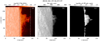 |
Fig. 1. Prominence observed by IRIS and the MSDP at the south-west limb of the Sun on 2018 April 19. The panels show (a) a slit-jaw image of the Mg II line (SJI 2796), (b) Hα intensity in the line centre observed by MSDP showing the solar disc used to co-align MSDP and IRIS maps, and (c) Hα ± 0.3 Å intensity observed by MSDP. The dashed lines in panel a mark the field of view of the IRIS raster. |
IRIS had a clockwise satellite rotation angle of 51 degrees, such that the solar limb was parallel to the y-axis of the instrument. We adopted this rotation angle for the co-alignment with the other instruments (AIA and MSDP). We note that it is easier to rotate AIA images than IRIS spectra data to minimise the influence of the rotation for the plasma diagnostics.
2.2. MSDP
To study the Hα line, we used the observations obtained with the MSDP spectrograph operating in the Meudon solar tower at the Paris Observatory. The observations were obtained between 12:05 UT and 16:35 UT, with sequences lasting 15 minutes each and an exposure time of 160 ms. The observations consisted of individual bands, and each of them covers a field of view of about 370 arcsec × 60 arcsec, with a pixel size approximately equal to 0.5 arcsec. Five adjacent bands recorded over 30 s allowed us to recover an image of the full field of view (370 arcsec × 270 arcsec) after processing the data with the MSDP software (Mein 1977, 1991; Mein et al. 2001). Our prominence was only covered by two individual bands, one covering the main part of the prominence and the other band covering the top. Each band is reconstructed from elementary spectral images of the entrance window (open slit) of the spectrograph obtained along a wavelength range ±0.7 Å. The scattered light was reduced by subtracting line profiles recorded outside the Sun in the close vicinity of the prominence. This method takes advantage of the fact that wavelengths are almost constant along lines perpendicular to the dispersion.
Our work focusses on the last sequence between 16:21 UT and 16:35 UT, which corresponds to an active phase of the prominence. The intensity in the Hα line centre allows us to see the whole prominence and the bright pattern of the chromosphere, which is very useful for co-alignment with the other instruments (Fig. 1b). In this panel, we did not correct the mean brightening between the bands to show the discontinuity between them. This highlights the rotation angle of ∼30 degrees between the direction of the band and the limb. For further analysis, we used the Hα maps with corrected intensity. The intensity and Doppler shift in each pixel in the prominence were computed in the Hα ± 0.3 Å range (Figs. 1c and 2b). We discuss how we proceeded for the co-alignment of MSDP and IRIS observations in detail. Table 1 summarises the details of the MSDP data. The MSDP Meudon observations of the prominence in Hα line are stored in the archive (LESIA08) of the Paris Observatory in Meudon.
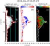 |
Fig. 2. Prominence diagnostic based on the MSDP observation. (a) Hα intensity at the line centre, (b) Doppler velocity, and (c) FWHM. The contours present the Hα prominence defined as Mask-Hα (see Sect. 4.7). The blue vertical lines in panel a are the two selected slit positions (A, B) used to analyse the profiles (Figs. A.3 and A.5) and for plasma parameter diagnostics (Table 3). The small horizontal lines are the positions corresponding to profiles A1–A15 and B1–B11. |
2.3. SDO/AIA
To study the spatio-temporal dynamics of the prominence with high-resolution, we used data obtained by the space-based mission Solar Dynamics Observatory (SDO; Pesnell et al. 2012). The Atmospheric Imaging Assembly (SDO/AIA; Lemen et al. 2012) instrument on-board SDO provides full-disc images that cover the solar atmosphere from the photosphere to the corona. The seven EUV channels (e.g., AIA 304 Å, AIA 171 Å, and AIA 193 Å) provide observations with a nominal spatial resolution of 1.2 arcsec. (pixel size 0.6 arcsec) and a temporal scale of 12 s. In our analysis, we used the AIA data obtained in the same time interval as the IRIS data.
We used an AIA 304 Å filter where the main emission comes from the He II line at 303.78 Å formed by a scattering of photons on ionised helium at a temperature of log T = 4.7 (Labrosse et al. 2010). Furthermore, a number of lines formed at coronal temperatures in the bandpass of 304 Å (Dere et al. 1997; Landi et al. 2012). However, they weakly affect the emission of cool prominences.
We also studied AIA 171 Å and AIA 193 Å images, formed at temperatures of log T = 5.8 and log T = 6.1, respectively. In these wavelengths, the cool plasma in the corona absorbs the background coronal emission and is visible in absorption. This was discovered by observations of the fine structures of a filament with the SST telescope (Scharmer et al. 2003) when compared with a TRACE image at 171 Å (Schmieder et al. 2004).
Prominences are well observed in the two filters of AIA 171 Å and 193 Å as absorption structures. In AIA 304 Å, prominences show a completely different appearance because they are seen in emission.
We used pre-processed SDO/AIA data, provided by the Joint Science Operations Center (JSOC2 that correspond to level-1.5. The SDO/AIA data exported from JSOC were mutually co-aligned with high spatial accuracy.
3. Evolution of the large-scale prominence in different temperatures
The MSDP, IRIS, and AIA instruments provide a view of the prominence at multiple temperatures (see Table 2). Due to opacity and different ionisation temperature effects, the prominence shape observed in each wavelength is different, revealing different structures.
3.1. Hα, Mg, and AIA 304 prominence
The global shape of the prominence observed in Hα and in IRIS SJI 2796 Å is very different (Figs. 1a and 2a). In Hα, the prominence consists mainly of two narrow and low columns with weak emission loops joining the column to the solar surface (Figs. 1c, 2a), while the IRIS prominence has a wide base of 100 arcsec parallel to the y-axis, and a height of about 50 arcsec (37 500 km). The top of the IRIS prominence is narrower, with one or two horns, depending on the time. A prominence with such an appearance was discussed in Wang et al. (2016). The differences in apparent morphology of prominences observed in different chromospheric lines have been discussed in the past. The optical thickness of the Mg II h or k line is ∼100 times greater than that of Hα (Ruan et al. 2019). This explains why all the low-density structures can be better seen in Mg II (Heinzel et al. 2015; Levens et al. 2016). Due to contrast issues, it is not possible to visualize the low emission structures in Hα.
The prominence in Hα is defined with ‘Mask-Hα’ (see Sect. 4.7). The Doppler shift and FWHM can be computed in the entire area limited by this mask. The area of the computed Doppler shifts corresponds to a large part of the IRIS prominence (Figs. 1 panel a, 2 panel b).
The IRIS SJI 2796 Å movie (Movie1) shows tremendous moving features during the five-hour observing time. During this time, the global structure of the prominence rises slowly (< 3 km s−1). The different periods of activity suggest the need for deeper analysis. In the IRIS SJI movie, we see major changes at the top of the prominence. The evolution of the prominence is shown in six panels in Fig. 3. At the beginning of the observation (14:15 UT), we observe long narrow loops joining the top of the prominence to the solar surface.
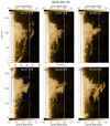 |
Fig. 3. Spatio-temporal evolution of the prominence intensity in Mg II slit-jaw 2796 Å images obtained by IRIS between 14:15 UT to 17:53 UT. The dashed vertical lines mark the IRIS raster field of view. The blue box in panel d defines the FOV used for detailed study of the velocity distribution (Fig. 9). The temporal evolution is available as an online movie (Movie1). |
Between 15:45 and 17:30 UT, the top appears as a relatively narrow column that displays some twisted motions. After turning to the north and south, at around 17:30 UT material from the top detaches, untwists, and unwinds to ultimately expand in a horizontal direction. Then, between 17:56 and 18:18 UT the material falls, following long loops towards the southern limb. We estimated the transverse flows along these loops to be less than 7 km s−1.
The dynamics of the prominence in AIA 304 movie (Movie2) has a similar behaviour to the prominence in the IRIS SJI 2796 Å movie, but with less contrast (Fig. 4). The fine structures, particularly at the top of the prominence, are not well observed. Their morphology changes rapidly and can only be resolved with the high spatial resolution of IRIS.
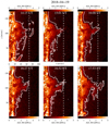 |
Fig. 4. Spatio-temporal evolution of the AIA 304 Å intensity observed between 14:15 UT and 17:53 UT. The vertical dashed lines mark the IRIS raster field of view. The overlaid contour corresponds to the contour of the IRIS SJI 2796, level = 1. The temporal evolution is available as an online movie (Movie2). |
The AIA 304 filter contains the He II 303.78 Å line, which is strongly affected by opacity effects, similarly to the Mg II lines. Prominences observed in this line look completely different to how they are seen in Hα but similar to what is seen in IRIS SJI 2796. The optical thickness of He II 303.78 Å is between 102 and 103 (Levens et al. 2016). This implies that we mainly observe the structures located at the front of the prominence. This allows us to observe weakly emitting structures not visible in Hα (Ruan et al. 2018), resulting in a more extended appearance of the prominence similar to what is seen in the IRIS SJI.
3.2. AIA prominence in 171 Å and 193 Å
In the SDO/AIA 171 Å and 193 Å images, the prominence absorbs the background coronal emission and appears as a dark column located in the centre of the prominence, oriented perpendicularly to the solar limb (Figs. 5 and 6). This absorption structure corresponds to the similarly shaped brightest region in the Hα MSDP image in Figs. 1b, c. The signal in AIA 171 is dominated by the Fe IX 171 Å line formed typically at log T = 5.9. However, this line is also sensitive to plasma at a lower temperature of log T < 5.6 in the prominence-to-corona transition region (Parenti et al. 2012). This is responsible for the diffuse emission surrounding the central absorption column, and the illumination of the extended loops joining the limb in the south and the loops surrounding the cavity. The SDO/AIA 193 channel emission is multi-thermal (log T = 6.1 − 7.3) and consists of contributions of several coronal lines of Fe XII and Fe XXIV. In this channel, the prominence is visible purely in absorption from the hydrogen and helium continuum opacity. The optical thickness of the continua at these wavelengths is comparable to the optical thickness of the Hα line, which is around unity (Schmieder et al. 2004; Anzer & Heinzel 2005). In the area surrounding the dark column, smaller columns are visible (Fig. 5). These wispy structures are less extended than in AIA 304 and are located inside the contour of the IRIS prominence. In the AIA 193 movie (Movie4), the top of the dark absorption column is seen to oscillate and change shape giving the impression of some twist.
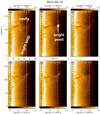 |
Fig. 5. Spatio-temporal evolution of the AIA 171 Å intensity observed between 14:15 UT and 17:53 UT. The vertical dashed lines mark the IRIS raster field of view. We note the presence of the cavity and long extended bright loop in (a), and a bright point in (b). The cavity is visible in all the panels, and the dark twisted column is surrounded with emission. The temporal evolution is available as an online movie (Movie3). |
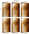 |
Fig. 6. Spatio-temporal evolution of the AIA 193 Å intensity observed between 14:15 UT and 17:53 UT. The vertical dashed lines mark the IRIS raster field of view. The overlaid contour corresponds to the contour of the IRIS SJI 2796, level = 1. The dark features (columns and fuzzy dark material) observed in the prominence correspond to the prominence observed in Hα. The temporal evolution is available as an online movie (Movie4). |
In the AIA 171 movie (Movie3), a part of a loop is seen surrounding the cavity (Fig. 6). At 15:01 UT a bright point is seen in the middle of the cavity. Is this bright point due to reconnection leading to activity in the prominence? It is not directly related to accelerated motions, and no emission is detected in the X-ray telescope (XRT) images from onboard the Hinode solar telescope (Golub et al. 2007). Later, more extended loops join the main body of the prominence to the solar surface. The top of the prominence becomes elongated in an orientation parallel to the limb, with material flowing towards the north and south. This gives also the impression of rotating structures.
4. Tornado-prominence dynamics
From the eighteen IRIS rasters obtained between 14:13 UT and 19:15 UT, we analysed the 3D dynamics of the activity in the prominence, with a particular focus on the top, which appears similar to a tornado at different times. The eighteen rasters include 32 spectra of Mg II h and k (Table 1). Of these spectra, 28 cover the prominence, while the first four spectra are on the disc or at the limb including spicules. Figure 7 shows an example of the Mg II k spectra through the prominence with a reconstructed map obtained using the integrated intensity of Mg II k.
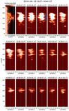 |
Fig. 7. Prominence spectra of raster 8. First row, left panel: reconstructed map using the integrated intensity of Mg II k line, five following panels: spectra along the slit in positions 10 to 14, second row: in positions 15 to 20, and bottom row: in positions 21 to 26. Upper left panel: the dot-dashed vertical lines represent the extreme slit positions (10 and 26) for which the spectra are shown in this figure. The dotted vertical lines are the two selected slit positions used to analyse the profiles and for plasma parameter diagnostics. In panels of the spectra, the vertical dashed blue line corresponds to the rest velocity. In the panel at 16:34:10 UT (slit position 12), the horizontal lines are the positions corresponding to profiles A1–A15 drawn in Fig. A.2. In the panel at 16:39:55 UT (slit position 23), the horizontal lines limit the domain where the profiles (B1–B11) are shown in Fig. A.4. The y-axis is in pixel units (1 pixel = 0.33 arcsec). |
4.1. Mg : Wavelength calibration method
To analyse the IRIS data, we first calibrated the wavelength of the Mg II spectra. We assumed that the average velocity of the photospheric line Ni I 2799.474 Å is equal to zero. A mean spectral profile of Ni I was created for the whole slit position located on the solar disk (first slit position). Using a spline interpolation, we computed the Ni I peak position.
We confirmed this calibration by computing an average spectral profile of the Mg II k line over the disc. The wavelength value of the mean spectral Mg II k profile dip is consistent with the nominal rest wavelength of the Mg II k line at 2796.35 Å (Pereira et al. 2013), and this confirmed the Ni I calibration result.
4.2. Mg : Gaussian fitting method
The observed Mg II spectra generally have no central reversal. Therefore, a Gaussian fitting procedure may be applied to retrieve the total intensity, full width at half maximum (FWHM), and Doppler shift. To avoid noise, we fitted Mg II k profiles with a single Gaussian profile when the peak amplitude was three times larger than the standard deviation of the background continuum intensity. The background continuum intensity was defined in the waveband of 5.09 Å, centred at 2811.23 Å.
To calculate velocity (v) with the Doppler effect, we used the following formula:
 (1)
(1)
where c is the speed of light, λobserved is the wavelength observed by IRIS, and λemitted is the wavelength emitted by plasma (theoretical wavelength).
We used the fitting parameters to determine the position of the line centre and the corresponding total intensity, FWHM, and Doppler shift. Figure 8 shows an example of these three quantities for raster 8.
 |
Fig. 8. Prominence reconstructed maps based on the IRIS spectra of Mg II k line (raster 8). (a) Integrated intensity of Mg II k line, (b) Doppler velocity, and (c) width (FWHM) of Mg II k line profile obtained by fitting the profiles with a single Gaussian function. The inner contour line (around x = 10 arcsec) corresponds to the solar surface defined as the level 0.6 Å of the FWHM of Mg II k line; the outer contour corresponds to Mask-Hα based on MSDP observations (see Mask-Hα in Fig. 2). This new contour defined by Mask-Hα (pixels on the disk) is used for the statistics of Mg II parameters in and out the Hα prominence (see Sect. 4.7). The blue dotted lines in panel a are the two selected slit positions (A, B) used to analyse the profiles (Figs. A.3 and A.5) and for plasma parameter diagnostics (Table 3). |
4.3. Mg : Quantile method
An alternative method to the Gaussian fitting is the quantile method (Kerr et al. 2015; Ruan et al. 2018). We only applied the quantile method for raster points where the peak intensity of the Mg II k line was at least three times larger than the standard deviation of the background continuum. The quantile method involves calculating the cumulative distribution function of the intensity of individual line profiles in a wavelength range. Based on the cumulative histogram of intensity, we calculated the 0.12, 0.5, and 0.88 quantile (percentile) parameters (respectively Q1, Q2, and Q3) considering a wavelength range of 2.04 Å centred on 2796.46 Å (this is the same wavelength interval as in the Gaussian fitting method). Based on the position of the line centre (peak), we created a map of peak intensity ( ). Again using Eq. (1), as in Sect. 4.2, we calculated the Doppler velocity. Then we calculated the FWHM as the wavelength distance between 0.12 (Q1) and 0.88 (Q3) quantile. The Gaussian and quantile methods give comparable results (Fig. 9).
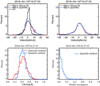 |
Fig. 9. Histograms of Doppler velocities for Hα and Mg II k lines inside the Hα prominence (left top panel) and in the whole Mg II prominence (right top panel), FWHM for Mg II k line and asymmetry of the Mg II k line computed with the quantile method. Hα prominence corresponds to pixels enclosed by the contour in Fig. 2 panel a and y-range from 60 to 137 arcsec. The whole Mg II k prominence is enclosed in the blue box presented in Fig. 3. The histograms are based only on the spectral profiles with an intensity larger than the noise. |
4.4. Evolution of the tornado prominence viewed in the IRIS raster
The movies (Movie1, Movie5) allow us to follow the evolution of the tornado in 3D with the associated Doppler shifts at a cadence of 16 min. This is a relatively low cadence for an active prominence. Figures 10 and 11 summarise the main behaviour of the tornado plasma with intensity and simultaneous Doppler-shift maps.
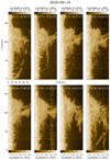 |
Fig. 10. Sample of integrated intensity maps in Mg II k line, each map being reconstructed from the 32 spectra of one raster, showing the evolution of the tornado at the top and the long loops connecting with the limb between 14:15 UT and 18:41 UT (rasters 1, 5, 7, 8, 9, 10, 13, and 17). |
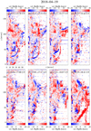 |
Fig. 11. Doppler velocity maps (Gaussian fitting) in Mg II k line computed from the spectra of the rasters observed by IRIS between 14:15 UT to 18:41 UT (rasters 1, 5, 7, 8, 9, 10, 13, 17). The temporal evolution is available as an online movie (Movie5). |
At the beginning of the observations, at around 14:13 UT, we see long alternating blueshifted and redshifted loops that link the top of the prominence to the disc. Between 15:27 and 16:27 UT, the top of the prominence extends to higher altitudes and exhibits changes in Doppler shift, with blueshifted and redshifted areas aligned perpendicularly to the limb. At around 16:07 UT, 16:35 UT, and 16:52 UT, a vertical pillar-like a tornado is observed and is seen to rapidly develop. In rasters 7, 8, and 9 (16:11 to 17:00 UT), redshifts and adjacent blueshifts are observed along the vertical pillar, simulating a tornado. At the end of raster 13 (around 17:53 UT), large flows with trajectories more or less parallel to the limb are observed from the top of the prominence, ejecting blueshifted material towards the north and redshifted material towards the south. Finally, the material moving along long the loops, joining the top of the prominence to the south limb, mostly shows redshifts. This flow is found to be moving away from the observer (18:41 UT, raster 17).
4.5. Co-alignment IRIS and MSDP data
A two-step procedure to co-align IRIS raster and MSDP data was undertaken. First, we reduced the IRIS SJI 2796 Å image resolution to the pixel size of MSDP (0.5 arcsec). Then, we used a cross-correlation method to co-align an IRIS SJI image with an MSDP intensity map of Hα at the line centre. The co-alignment was done with the solar disc using the structures of the network. We obtained a precision of alignment better than 1 arcsec between the IRIS SJI and MSDP images.
In the second step, we co-aligned IRIS SJI 2796 Å images with IRIS raster data. To achieve this, we used the IRIS raster integrated-intensity maps in the Mg II k line and reduced the SJI resolution to the raster image. Then, we used the fiducial as a spatial reference in the rasters and a cross-correlation method to align the SJI and raster image. A cross-correlation method was applied in the full FOV of the Mg II k raster intensity image. Due to the fast evolution of the prominence, we chose the last SJI image obtained during the rastering process, which corresponds better to the prominence; the first one corresponds to the disc and the low part of the prominence. The accuracy of the co-alignment is better than 2 arcsec. The result is shown in Figs. 1a–c.
4.6. Hα Doppler shifts
In each pixel of the MSDP prominence field of view, a Hα profile is retrieved and Doppler shifts were computed using a bisector method. Hα profiles in prominences are relatively narrow compared to profiles on the disc, but they are broader than synthetic profiles obtained by radiative transfer codes from Ruan et al. (2018, 2019).
The Doppler shifts were determined as follows: we considered the blue and the red points in a Hα profile (I(λb) and I(λr), respectively), such as I(λb) = I(λr) and λr–λb = 0.6 Å. The shift of the middle of the 0.6 Å wavelength interval compared to the rest value represents the Doppler shift of the pixel. The zero velocity was obtained by assuming that the sum of all the velocities in the prominence is null. Doppler-shift maps were obtained every 30 s (see an example in Fig. 2b and in Appendix A (Fig. A.1)). Large sections of the prominence are seen to have coherent velocities. This has previously been discussed in earlier works Schmieder et al. (2010), Ruan et al. (2018).
4.7. Mask definition for Mg prominence
To compare the spatio-temporal evolution and physical properties of the prominence viewed in Hα and Mg II, we used the IRIS raster data and MSDP observations. We created a mask to remove the solar disc and the background due to scattered light and noise. First, we defined the position of the solar limb. Based on the FWHM map of Mg II, we defined a solar surface as level 0.6 Å of the FWHM of the Mg II k line. In Fig. 8, the inner contour line (around x = 10 arcsec) corresponds to the solar surface. All points with an FWHM larger than 0.6 Å (the left side from the contour line) belong to the solar disc. The outer edge of the mask corresponds to the contour of the prominence in the Hα intensity map defined from the MSDP observation (Mask-Hα).
The mask is obtained directly from Hα profiles in each pixel. Profile intensities need to be much greater than the noise, so a parameter M is defined as the difference between the intensity in line centre and the average intensity in wings at +0.6 Å and −0.6 Å. When this parameter is too low (here, M lower than 10 in camera arbitrary units), the pixel is declared out of the prominence. This value is small compared to the M values exceeding 250 in the brightest parts of prominence. However, we see that possible fluctuations due to noise from pixel to pixel do not appear in velocity maps (Fig. 2b), even in the weak parts of the prominence, close to the mask. Therefore, the Mg II prominence is defined as the region between the solar limb (left line in Fig. 8) and the outer edge of prominence (right contour in Fig. 8).
4.8. Comparison of Hα and Mg Doppler shifts and FWHM
The spectral analysis of the Mg II lines shows alternating red and blue enhancements in the wings as one moves along the slit (Fig. 7). We note that these enhancements are coherent over a distance of a few arcsec along the slit. The structures along the slit are narrower at the top of the prominence.
The histograms of the Doppler velocities for Hα and Mg II k show that the Doppler shifts of both lines are of the same order of magnitude, however the Doppler shifts in Mg II can reach 30 km s−1 in a few pixels (Fig. 9). We note that the histogram of the Hα Doppler velocities shows more blueshifted points compared to the histogram of the Doppler velocities of the Mg II lines, which show more redshifted points. This difference is intrinsic to the definition of the rest velocities. For Hα, we computed the rest velocity using the mean value of all the velocities in the prominence. For the wavelength calibration of Mg II lines, we used the photospheric line Ni I (see Sect. 4.1). The Mg II histogram is for raster 8, which was obtained in 16 min, while the Hα dopplergram was obtained in under 30 s.
The FWHM of the Mg II k line is computed via Gaussian fitting and the quantile method. The two results are in agreement with a FWHM between 0.2 and 1 Å (Fig. 9). With the quantile method, we show that a fraction of the profiles are asymmetric, meaning that their velocities are in reality higher than the computed ones (Fig. 9). This effect is also discussed in Peat et al. (2021).
Figures 12a–d show the probability density functions for the Mg II k line in the prominence inside and outside the Hα contour, respectively. In Fig. 12a, we note that the integrated intensity is roughly proportional to the width of the Mg II line profile, with this correlation plateauing for medium width profiles for a wide range of integrated intensities. High integrated intensities correspond to wide profiles with a FWHM reaching 0.8 Å. In Fig. 12c, there is a weak correlation. Weak intensities are observed with profiles of any width, but more profiles with an FWHM of 0.2 Å have a weak intensity. For the Mg II prominence inside the Hα contour, there are no large Doppler shifts. The maximum Doppler shift is around 10 km s−1. Outside of the Hα contour, the narrow profiles exhibit large Doppler shifts of ±25 km s−1. For Hα profiles, there is a correlation between intensity and FWHM. Therefore, relatively narrow profiles (0.6 Å) have a lower intensity than wider profiles (1 Å) (Fig. 12 panels e). In panel f, we note that narrow profiles have Doppler shifts between −5 km s−1 and +5 km s−1, very few points reach a higher velocity. This demonstrates that wide Hα profiles are created by the integration of multiple emitting structures with different velocities along the LOS. This results in wide line profiles. Broad Hα profiles are the signature of the integration of many threads along the LOS.
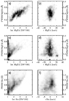 |
Fig. 12. Probability density functions (PDFs) for Mg II k line parameters for the area between the limb and the outer edge of the Hα prominence contour, y-range from 60 to 137 arc in Fig. 8: (a) intensity versus FWHM, (b) Doppler velocity versus FWHM; outside of the Hα contour, (c) intensity versus FWHM, (d) Doppler velocity versus FWHM; PDFs for Hα line parameters, (e) intensity versus FWHM, and (f) Doppler velocity versus FWHM. The PDF values are plotted in linear scale. |
Plasma parameters of the prominence in raster 8 from non-LTE radiative transfer models.
4.9. Magnetic field configuration
The Doppler-shift maps in Fig. 11 clearly show blueshift and redshift zones parallel to a vertical axis at the top of the prominence (see between 16:11 and 16:27 UT). This suggests twist and rotation. The prominence, when viewed in intensity, has a very classical global morphology with one or two horns at the top (Fig. 10). However, if we zoom in on the top or look at the IRIS SJI movie, we see distinctly horizontal sub-structures at the top of the vertical column. These are particularly apparent when material escapes from one of the sides of the top of the prominence (Fig. 13, bottom panels). This allows us to conclude that the magnetic configuration of this prominence is similar to classical prominences defined by a flux rope (Aulanier & Démoulin 1998; Aulanier & Schmieder 2002; van Ballegooijen 2004). Flux rope is commonly represented by twisted magnetic field lines, found by linear force free field extrapolation (Fig. 13 top panels). Filaments are supported by such a flux rope (FR) overlaid by arcades. The idea is that the plasma is located in the dips of the FR and represents the filament viewed in Hα. The magnetic field lines were obtained for another filament as it was crossing the limb of Aulanier & Schmieder (2002) (Fig. 13, top left panel). Above the limb when only the dips are drawn, we see two horns with an accumulation of horizontal fine structures like the fine structures in our prominence (top right panel). This kind of interpretation was confirmed by the models of Gunár et al. (2018), which include radiative transfer. Gunár et al. (2018) were able to mimic a real prominence viewed from the top and the side with horizontal dips. An MHD view of a prominence does not consider the plasma in the prominence itself. With IRIS spectroscopy, we explored the characteristics of the plasma loading the dips.
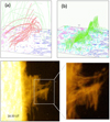 |
Fig. 13. (a) Reconstructed filament with flux rope field lines (red lines) overlaid by arcades (green lines). These field lines are obtained from an LMHD extrapolation of an observed photospheric magnetogram for a different prominence. (b) Dips in the magnetic field lines (green lines; adapted from Aulanier & Schmieder 2002). Bottom panels: magnified view of the tornado-like structure showing an accumulation of fine horizontal structures, similarly to the green lines in (b). |
5. Plasma characteristics from observations and theory
To analyse the plasma characteristics of the prominence using Mg II lines, we chose two slit positions in the Mg II prominence: the main body (slit 12, 16:34 UT) and the top (slit 23, 16:39 UT) representative of the physical state of the prominence (Fig. 8 panel a vertical dashed lines). Similar positions are selected in the Hα image with the coordinates x = 24 and 46 arcsec (Fig. 2, panel a).
5.1. Mg integrated intensity, Doppler shifts, and FWHM
Figures 14 and 15a–c show the integrated intensity in erg s−1 cm−2 sr−1, the Doppler shifts in km s−1, and the FWHM in Å, respectively, for the Mg II k line along the slits 12 and 23, respectively. The prominence is located along the y-axis between pixels 250 and 400, which corresponds to a width of around 50 arcsec at a height of 20 arcsec. Structures of high intensity are observed along the slit reaching 5 to 6 × 10⁴ erg s−1 cm−2 sr−1, while the width of the top along slit 23 is narrower at around 33 arcsec, with a mean maximum integrated intensity of 2 × 10⁴ erg s−1 cm−2 sr−1. The raster spectra in Fig. 7 show accumulations of narrow structures (around 2000 km), with the smallest reaching one or two pixels (dimension of the order of 250 km to 500 km). In Figs. 14 and 15, the Doppler shifts range between −5 and 15 km s−1, with three main structures of 25 to 35 pixels (8–10 arcsec.) in the main part of the prominence whereas the top has narrow velocity structures of around 1.5 to 2 arcsec. The FWHM is 0.3 Å at the edge of the prominence but reaches 0.4 Å at the top and 0.5 Å in the body. The Doppler-shift structure includes many fine structures with coherent velocities, as shown in Fig. 11.
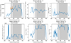 |
Fig. 14. Prominence body characteristics: (top panelsfrom left to right) Mg II k observed integrated intensity, Doppler shift, and FWHM along slit 12; (bottom panels from left to right) non-LTE model results along slit 12, mean electron density, τ(Mg II k), and τ(H α). The grey areas correspond to pixels where the observed profiles in Mg II cannot be correctly fitted with the grid of profiles derived by the non-LTE radiative transfer code. The red arrows indicate the points in Table 4. |
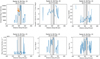 |
Fig. 15. Prominence tornado characteristics: (top panels from left to right) observed integrated intensity, Doppler shift, and FWHM along slit 12; (bottom panels from left to right) non-LTE model results along slit 12, mean electron density, τ(Mg II k), and τ(H α). The grey areas correspond to pixels where the observed profiles in Mg II cannot be correctly fitted with the grid of profiles derived by the non-LTE radiative transfer code. The red arrows indicate the points in Table 4. |
5.2. Mg and Hα profiles
Along the two slits, we chose individual pixels with a step of one arcsec at the top (slit 23) (B1–B11) where the structures look narrow and a step of 5 arcsec in the main body (slit 12) (A1–A15). Table 3 summarises the characteristics of these profiles. This table allows us to compare these quantitative values with the theoretical values of synthetic profiles obtained from the radiative transfer models of Levens & Labrosse (2019).
The Mg II and Hα profiles from the top of the prominence (B1–B11) at 16:25 UT can be seen in Figs. A.4 and A.5. The profiles from the main part of the prominence (A1–A15) can be seen in Appendix A (Figs. A.2 and A.3). The Mg II k profile intensity peaks reach 8 to 12 × 104 erg cm−2 s−1 sr−1 Å−1 in the body (points A1–A15) and 5 to 10 × 104 erg cm−2 s−1 sr−1 Å−1 at the top (points B1–B11). The mean ratio between the integrated intensities of Mg II k versus Mg II h is around 1.4 for our sample of points (between 1.38 and 1.55, with an exceptional value of 1.76). This value is typical of prominences (Levens et al. 2016; Ruan et al. 2018).
Figures A.3 and A.5 show a set of example MSDP prominence profiles at 16:25 UT from the main part (A1–A15) and the top part (B1–B11), respectively. The profiles are mostly seen to be wide with a FWHM between 0.653 Å and 0.911 Å (see Table 3).
The profiles at the top are narrower than in the body because the LOS could cross fewer structures. In the main body, the LOS crosses many structures, each of them having different velocities, resulting in the broadening of the line profiles. The Hα profiles are all wide between 0.5 and 0.8 Å. This results in a larger FWHM than those predicted by 1D models. Single structures cannot be resolved with the spatial resolution of the MSDP spectrograph. The Hα line is usually considered as an optically thin line, meaning that many structures are integrated along the LOS (Wiik et al. 1992). However, the Hα line may also be optically thick in some cases. The observed FWHM can be larger than this when predicted by 1D models for various reasons, especially unresolved structures or optically thick structures with a high speed gradient.
5.3. Interpretation with a 1D radiative transfer code
Levens & Labrosse (2019) developed a 1D non-LTE radiative transfer code to understand how physical conditions inside a prominence slab influence shapes and properties of emergent Mg II line profiles. This code includes two types of model atmospheres: isothermal and isobaric; and a prominence-corona transition region (PCTR). Using this code, they computed a grid of 1007 models, 755 of which contain a PCTR. Mg II spectra were computed to demonstrate the influence of the physical parameters of the prominence on the emergent spectra (e.g., temperature and geometric thickness). In particular, they obtained good correlations between the Mg II k line intensities and the intensities of hydrogen lines and emission measurements. Prominence parameters can be retrieved from comparing these synthetic profiles with observations. Mg II is ionised for a temperature higher than Tmax = 30 000 K. Therefore, most prominences emitting in Mg II lines are cold (T < Tmax), low-pressure, and optically thick structures. Their results agree with previous studies (Heinzel et al. 2014, 2015; Jejčič et al. 2018).
5.4. Correlation between Mg and Hα lines and emission measures
First, we used the global results obtained with the grids of models concerning the integrated intensities of Mg II (E(Mg II)) and Hα (E(Hα)) and the emission measure (EM). The gas pressure is an input parameter, so it changes depending on the model. The graphs in Fig. 16 contains all 1007 models of the grid. The inputs of the pressure range from 0.1 to 1 dyne cm−2. Assumptions on the geometrical thickness and temperature of the structures were made, restricting it to thicknesses of 1000–5000 km and temperatures from 6000 K to 20 000 K, with a constant microturbulence equal to 5 km s−1.
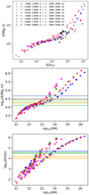 |
Fig. 16. Models of radiative transfer for two parameters: temperature between 6000 K and 20 000 K, and geometrical thickness between 1000 km and 5000 km. Top panel: correlation between integrated intensity of Mg II k versus Hα. The black stars represent the observations (see Table 3). Middle panel: correlation between integrated intensity and EM for Mg II k. Bottom panel: correlation between integrated intensity and EM for Hα. The horizontal lines correspond to the extreme values measured in the prominence body (blue), at the edge (green), and at the top (orange). |
Figure 16 (top panel) shows the variation of E(Mg II) versus E(Hα) obtained with this sample of theoretical models. The observational points of Table 3 have been included in the figure. We found a generally good agreement with the theoretical points, which means that the co-alignment of the spectra (IRIS and MSDP) have been done correctly. Figure 16 (middle and bottom panels) shows the correlations between E(Mg II k) and EM, and between E(Hα) and EM. We can get an approximate value of EM corresponding to the observations. The values of E(Mg II k), E(Mg II h), and E(Hα) in Table 3 concern the top and the main parts of the prominence. We separated the main body into two parts: the edge of the prominence and the central part of the prominence. Two sets of horizontal lines, in green and blue, respectively, were drawn bounding the extrema of these regions, whereas the extrema of the top part are bound by orange lines.
From Fig. 16 (middle), the edge and top are found to have a log(EM) of between 22.1 and 23.8. From Fig. 16 (bottom), they are found to have a log(EM) of 22.5 to 23.5. For the body, Fig. 16 (middle) gives a log(EM) of 23 to 24.2, and Fig. 16 (bottom) gives a log(EM) of 23.5 to 24.4. The agreement between these values is satisfactory. The EM is slightly higher for Hα than for Mg II.
If we estimate that the edge or top of the prominence have a geometrical thickness (D) of less than 3000 km, then the values for log(EM) plateau, and the uncertainty becomes large for the electron density (3 × 10⁹ − 3 × 1010 cm−3). For the central part of the prominence, where D is around 3000 km, the uncertainty is less significant. The estimate of electron density is around 1010 ± 0.3 × 1010 cm−3.
5.5. Observed and synthesised profiles
We used the recent results of Peat et al. (2021) derived from the synthesised profiles obtained with their large database of models. Their computed line profiles include the two classic shapes of Mg II h&k profiles (reversed and single peaked). They argue that matching a line profile by comparing the integrated intensities and FWHM of the synthesised profiles to that of the observations is not enough to take into account the two possible kinds of line profiles. They instead compared the computed and observed line profiles point by point in wavelength space. It is computationally faster to vectorise and fit the whole raster (i.e., all of the pixels) at once rather than doing it pixel by pixel.
The procedure is first and foremost an RMS minimisation routine. The code will always find a fit that it believes to be best, regardless of what data it is given. However, Peat et al. (2021) introduced a test to quantify the level of agreement between the observed profile and the computed best-fit profile. This leads to the use of two filters (applied ad hoc in the routine) – a prominence filter and a bad-fit filter. The former filters out noise and the solar limb, leaving only prominence material, and the latter filters bad fits (i.e., pixels where the agreement between the best modelled profile and the observed profile is not high enough). These two filters have to work together, as ‘good fits’ are found in the noise by the simple metric used by the bad-fit filter (an RMS cut-off). The ‘best fit’ found in the noise is usually a low-intensity, single-peaked, low-FWHM profile. The RMS here is below that of the RMS cut-off because the noise itself is so low that the RMS is low even although the fit is bad.
High-intensity profiles are fitted with a mix of double and single peaks, depending on the profile we are fitting to. The best fits are actually from high intensity single peaks and low FWHM. In Fig. 17 (left panel), we present the map of the points where the best fits are obtained. We note that they are at the edge of the Mg II prominence.
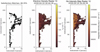 |
Fig. 17. Theoretical results of the non-LTE radiative transfer code using the fitting profile method. Left panel: pixels where the fitting is satisfactory; middle panel: electron density map; right panel: intensity in Hα according to the models. |
5.6. Electron density and optical thickness
The electron density map was computed with the Levens and Labrosse radiative transfer code for all the pixels, even with a relatively low weight for the pixels where the best fit was not found (Fig. 17 middle panel). Using the good co-alignment between the MSDP maps and IRIS rasters, we show an Hα intensity map with a superimposed electron density map (Fig. 17, right panel). The red contour limits the Hα prominence (brown). By comparing maps in the right and left panels, we note that the Hα prominence almost corresponds to points where the fit of Mg II lines was not correct due to their complex profiles.
In order to obtain parameter quantitative values concerning the prominence and its top, we analysed the theoretical results obtained for the two selected slit positions; for example, mean electron density, optical thickness of Mg II k, and optical thickness of Hα (Figs. 14 and 15 – bottom panels from left to right, and Table 3). For these pixels, we compare the values of the ratio between the Mg II k and h integrated intensities computed with the models and observed. It is globally in agreement, except for some values exceeding typical ratio values for prominence, for example around 1.4 (Fig. 18). Profiles of the Mg II h line show similar shapes to Mg II k profiles (not shown in the paper). The gaps in the data are filtered points that the filter found to not be prominence material.
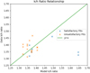 |
Fig. 18. Ratio relationship between the Mg II h and k integrated intensities computed by the models versus the observations (data). |
In a first step, we analysed the electron density for pixels in the Hα prominence (inside Hα mask in Fig. 2), and in a second step we analysed for pixels outside the Hα mask but within the Mg II prominence.
5.6.1. Electron density for pixels inside Hα prominence
The Mg II k profiles of the central part of the prominence have a wide FWHM and a complex profile (Figs. A.2 and A.4), therefore they could not be fitted by any synthesised profile (Table 3).
All synthesised profiles have a FWHM less than 0.3 Å. As we see in Figs. 14 and 15 panels c, the FWHM exceeds this threshold and is coloured in grey. This means that the fit was qualified as ‘bad’ and the results from the non-LTE radiative transfer code are not reliable in these pixels. A good fit is mainly possible at the edges and at the top of the prominence. Figure 17 illustrates this well. Due to the ill-matched profiles, we cannot use the code to deduce the electron density in the thick part of the prominence that is spatially correlated with the Hα prominence. Only the first method based on correlations (Sect. 5.4) can be used to derive ranges of possible values of the electron density.
With the fitting profile method, we retrieved similar results to those obtained with the statistical method for the mean electron density. However, if we concentrate on a few pixels where the fitting was selected to be ‘good’ we obtain the following results (see Table 4). At the top, the electron density is between 1.8 × 10⁹ and 2.66 × 1010 cm−3. At the edge of the central part of the prominence, we only have two values: 3.7 × 10⁹ and 1.66 × 1010 cm−3. The electron density is small (less than 1010 cm−3) in models with a transition region containing plasma at high temperatures. The profiles obtained in pixels at the top or edge of prominences are fitted either by isothermal or PCTR models. In the isothermal models, the electron density at the edge of the prominence is higher (> 1010 cm−3) than in PCTR models. Points A3 and B2, which are located at the edge of the prominence, have the highest electron density values (1.66 and 2.68 × 1010 cm−3) compared to points that are closer to the central part of the prominence. For a given geometrical thickness, the electron density should commonly decrease to the edge of a prominence. An increase in electron density can be achieved by an enhanced ionisation in this region due to strong irradiation from the coronal environment. The radiation does not fully penetrate into deeper layers of the prominence, therefore the ionisation degree and electron density can be lower in the inner parts contrary to what was the case for previous concepts (Engvold et al. 2008).
5.6.2. Electron density for pixels outside the Hα prominence
The trend of the electron density to increase at the top (tornado-like) is confirmed for pixels outside of the Hα prominence, analysed with the fitting method (Fig. 15 pixel C at x = 345). Such pixels have Mg II line profiles with a very low intensity, which are well fitted with synthesised profiles obtained with PCTR models leading to a very high electron density reaching 1011 cm−3 and a high temperature above 20 000 K. A few pixels, such as pixel C (shown in Table 4), have those characteristics. Such a higher density compared to the inner prominence density is unusual and is discussed in the following section. This possibility was already mentioned in a previous work (Wiik et al. 1992).
The optical thickness of the Mg II h line (τMg IIh) is equal to low values (around 0.6 to 3) or to very high values between 23 and 32. The optical thickness of the Mg II k line (τMg IIk) is equal the double of the τMg IIk, the low values between 1.1 and 4 or very high values between 45 and 63 according to the model solution. The low values correspond to pixels at the edge where the plasma is hot (around 23 700 K), while the high τ values correspond to isothermal models. For PCTR models, the temperature is high, and Mg II becomes a very thin line; this may explain the low optical thickness in that case. Otherwise, the optical thickness of the order of 30 to 60 is typical in prominences (Levens et al. 2016). In any case, the mean pressure is always between 0.01 and 0.05 dyne cm−2, which are low values.
6. Discussion and conclusion
We present the data concerning a tornado-like prominence observed on April 19, 2018 with three instruments (SDO/AIA, IRIS, MST/MSDP). The top of the prominence is active and shows twist and rotation in the AIA 171 and IRIS SJI 2796 movies, suggesting evidence of a tornado.
We carefully analysed the evolution of the prominence intensity and velocity using IRIS spectra and SJIs. The SJIs show that the top of the prominence consisted of horizontal fine structures where material was alternately going away from or towards the sky plane. We noted the formation of blobs at the top, which escape along long field lines with large transverse velocities. We mentioned the similarity of this prominence with previous LFFF magnetic extrapolations obtained for different prominences (Aulanier & Schmieder 2002). In their extrapolation long twisted field lines are part of a flux rope simulating the prominence surrounded by arcades. The prominence is represented by the dips in the field lines. We suggest that the leakeage of the blobs occur along the flux rope magnetic field lines or arcades. With such a configuration, it is difficult to infer that the tornado could really turn on itself. Therefore, the Doppler shifts derived from the spectra of IRIS showing adjacent blueshifts and redshifts in vertical areas at the top would be interpreted as counter-streaming flows and not rotation.
The second part of the paper concerns the plasma characteristics in the prominence and its top. The results are unexpected and require discussion. Plasma parameters were obtained using the results of an non-LTE radiative transfer code (Levens & Labrosse 2019). We adopted two methods. The first method is to use statistics data based on two observables, such as integrated intensity and the FWHM of Mg II and Hα lines in each pixel. The second method is based on the fitting of Mg II h and k line profiles with synthesised profiles using the radiative transfer code. The first method has already been used in previous studies of prominences (Wiik et al. 1992; Heinzel et al. 2015; Jejčič et al. 2018; Ruan et al. 2019). From the theory, we found the variation of the integrated intensity of Mg II and Hα lines according to the emission measure (EM). Then, we were able to estimate the electron density according to assumptions concerning temperature and geometrical thickness. Electron density increases with the geometrical thickness and decreases with temperature. With an assumption of narrower geometrical thickness (D) for the low integrated intensity domain (log E(Mg II k) = 4–4.5), all the curves are overlapping. Therefore, we have no precise solutions for the top of the prominence. For higher integrated intensities, we found an electron density value around 1010 ± 0.3 × 1010 cm−3. Such intensities are found in the main part of the prominence.
The second method based on fitting profiles was much more powerful, principally for the top of the prominence. We concentrated on the narrower profiles at the top and at the edge of the prominence with low intensity, part which is not visible in Hα. We found that the electron density at the top could reach 1011 cm−3. This value is larger than the value for the inner part of the prominence (1010 cm−3) using prominence-corona-transition-region (PCTR) models. We explained this as being due to high ionisation at the edge leading to very high electron density (Peat et al. 2021). These points are located at the top of the prominence.
The plasma in these points would be in an ionisation phase due to radiation, and this would justify the high electron density with a high temperature. It could concern the formation by condensation and heating of the plasma at the top (Luna et al. 2012; Claes et al. 2020). Claes et al. (2020) found that at small scales a strong fragmentation during the formation of prominence plasma, which may correspond to the fine structures at the top of our prominence. In a first phase, this material would appear to be flowing over the spine of the prominence. This would explain why we see tornadoes only when prominences are passing over the limb. In a second phase, blobs would form and flow along long field lines of the flux rope.
1D non-LTE models have limitations for the interpretation of broad profiles, which may be the result of double or triple structures along the LOS. The broad profiles could also be due to high microturbulence. Ruan et al. (2019) used high microturbulence as a proxy of multi-structure velocities. A 2D non-LTE radiative model would be suitable to fit more profiles with wide FWHMs.
Movies
Movie 1 associated with Fig. 3 Access Supplementary Material
Movie 2 associated with Fig. 4 Access Supplementary Material
Movie 3 associated with Fig. 5 Access Supplementary Material
Movie 4 associated with Fig. 6 Access Supplementary Material
Movie 5 associated with Fig. 11 Access Supplementary Material
Acknowledgments
We thank the observation team at the Meudon solar tower for providing the MSDP data: Pierre and Nicole Mein, Daniel Crussaire and Guiping Ruan. We thank Clara Froment for chairing a fruitful discussion of our observations during the COSPAR 2021 session. Figure 13 has been provided by Guillaume Aulanier. This study benefited from financial support from the Programme National Soleil Terre (PNST) of the CNRS/INSU, as well as from the Programme des Investissements d’Avenir (PIA) supervised by the Agence nationale de la recherche. The work of KB is funded by the LabEx Plas@Par which is driven by Sorbonne Université. AWP acknowledges financial support from the Science and Technology Facilities Council (STFC) via grant ST/S505390/1. NL acknowledges support from STFC grants ST/P000533/1 and ST/T000422/1.
References
- Anzer, U., & Heinzel, P. 2005, ApJ, 622, 714 [NASA ADS] [CrossRef] [Google Scholar]
- Aulanier, G., & Démoulin, P. 1998, A&A, 329, 1125 [Google Scholar]
- Aulanier, G., & Schmieder, B. 2002, A&A, 386, 1106 [NASA ADS] [CrossRef] [EDP Sciences] [Google Scholar]
- Claes, N., Keppens, R., & Xia, C. 2020, A&A, 636, A112 [EDP Sciences] [Google Scholar]
- Culhane, L., Harra, L. K., Baker, D., et al. 2007, PASJ, 59, S751 [NASA ADS] [CrossRef] [Google Scholar]
- De Pontieu, B., Title, A. M., Lemen, J. R., et al. 2014, Sol. Phys., 289, 2733 [NASA ADS] [CrossRef] [Google Scholar]
- Dere, K. P., Landi, E., Mason, H. E., Monsignori Fossi, B. C., & Young, P. R. 1997, A&AS, 125, 149 [NASA ADS] [CrossRef] [EDP Sciences] [Google Scholar]
- Dudík, J., Aulanier, G., Schmieder, B., Bommier, V., & Roudier, T. 2008, Sol. Phys., 248, 29 [NASA ADS] [CrossRef] [Google Scholar]
- Engvold, O., Hirayama, T., Leroy, J. L., Priest, E. R., & Tandberg-Hanssen, E. Hvar Reference Atmosphere of Quiescent Prominences (Springer), 363, 294 [CrossRef] [Google Scholar]
- Golub, L., Deluca, E., Austin, G., et al. 2007, Sol. Phys., 243, 63 [NASA ADS] [CrossRef] [Google Scholar]
- Gouttebroze, P., Heinzel, P., & Vial, J. C. 1993, A&AS, 99, 513 [NASA ADS] [Google Scholar]
- Gunár, S., & Mackay, D. H. 2015, ApJ, 812, 93 [NASA ADS] [CrossRef] [Google Scholar]
- Gunár, S., & Mackay, D. H. 2016, A&A, 592, A60 [NASA ADS] [CrossRef] [EDP Sciences] [Google Scholar]
- Gunár, S., Heinzel, P., & Anzer, U. 2007, A&A, 463, 737 [NASA ADS] [CrossRef] [EDP Sciences] [Google Scholar]
- Gunár, S., Heinzel, P., Anzer, U., & Schmieder, B. 2008, A&A, 490, 307 [NASA ADS] [CrossRef] [EDP Sciences] [Google Scholar]
- Gunár, S., Dudík, J., Aulanier, G., Schmieder, B., & Heinzel, P. 2018, ApJ, 867, 115 [NASA ADS] [CrossRef] [Google Scholar]
- Heinzel, P., Vial, J.-C., & Anzer, U. 2014, A&A, 564, A132 [NASA ADS] [CrossRef] [EDP Sciences] [Google Scholar]
- Heinzel, P., Schmieder, B., Mein, N., & Gunár, S. 2015, ApJ, 800, L13 [NASA ADS] [CrossRef] [Google Scholar]
- Jejčič, S., Schwartz, P., Heinzel, P., Zapiór, M., & Gunár, S. 2018, A&A, 618, A88 [NASA ADS] [CrossRef] [EDP Sciences] [Google Scholar]
- Karpen, J. T., Antiochos, S. K., Hohensee, M., Klimchuk, J. A., & MacNeice, P. J. 2001, ApJ, 553, L85 [NASA ADS] [CrossRef] [Google Scholar]
- Kerr, G. S., Simões, P. J. A., Qiu, J., & Fletcher, L. 2015, A&A, 582, A50 [NASA ADS] [CrossRef] [EDP Sciences] [Google Scholar]
- Labrosse, N., Heinzel, P., Vial, J.-C., et al. 2010, Space Sci. Rev., 151, 243 [Google Scholar]
- Landi, E., Del Zanna, G., Young, P. R., Dere, K. P., & Mason, H. E. 2012, ApJ, 744, 99 [Google Scholar]
- Leenaarts, J., Pereira, T. M. D., Carlsson, M., Uitenbroek, H., & De Pontieu, B. 2013a, ApJ, 772, 89 [NASA ADS] [CrossRef] [Google Scholar]
- Leenaarts, J., Pereira, T. M. D., Carlsson, M., Uitenbroek, H., & De Pontieu, B. 2013b, ApJ, 772, 90 [NASA ADS] [CrossRef] [Google Scholar]
- Lemen, J. R., Title, A. M., Akin, D. J., et al. 2012, Sol. Phys., 275, 17 [Google Scholar]
- Levens, P. J., & Labrosse, N. 2019, A&A, 625, A30 [NASA ADS] [CrossRef] [EDP Sciences] [Google Scholar]
- Levens, P. J., Schmieder, B., Labrosse, N., & López Ariste, A. 2016, ApJ, 818, 31 [NASA ADS] [CrossRef] [Google Scholar]
- Li, L., Zhang, J., Peter, H., et al. 2016, Nat. Phys., 12, 847 [NASA ADS] [CrossRef] [Google Scholar]
- Luna, M., Karpen, J. T., & DeVore, C. R. 2012, ApJ, 746, 30 [Google Scholar]
- Luna, M., Moreno-Insertis, F., & Priest, E. 2015, ApJ, 808, L23 [NASA ADS] [CrossRef] [Google Scholar]
- Mackay, D. H., Karpen, J. T., Ballester, J. L., Schmieder, B., & Aulanier, G. 2010, Space Sci. Rev., 151, 333 [Google Scholar]
- Magara, T. 2007, PASJ, 59, L51 [NASA ADS] [CrossRef] [Google Scholar]
- Mein, P. 1977, Sol. Phys., 54, 45 [NASA ADS] [CrossRef] [Google Scholar]
- Mein, P. 1991, A&A, 248, 669 [NASA ADS] [Google Scholar]
- Mein, N., Schmieder, B., DeLuca, E. E., et al. 2001, ApJ, 556, 438 [NASA ADS] [CrossRef] [Google Scholar]
- Okamoto, T. J., Tsuneta, S., & Berger, T. E. 2010, ApJ, 719, 583 [NASA ADS] [CrossRef] [Google Scholar]
- Orozco Suárez, D., Asensio Ramos, A., & Trujillo Bueno, J. 2012, ApJ, 761, L25 [NASA ADS] [CrossRef] [Google Scholar]
- Parenti, S., Schmieder, B., Heinzel, P., & Golub, L. 2012, ApJ, 754, 66 [Google Scholar]
- Peat, A. W., Labrosse, N., Schmieder, B., & Barczynski, K. 2021, A&A, 653, A5 [NASA ADS] [CrossRef] [EDP Sciences] [Google Scholar]
- Pereira, T. M. D., Leenaarts, J., De Pontieu, B., Carlsson, M., & Uitenbroek, H. 2013, ApJ, 778, 143 [NASA ADS] [CrossRef] [Google Scholar]
- Pesnell, W. D., Thompson, B. J., & Chamberlin, P. C. 2012, Sol. Phys., 275, 3 [Google Scholar]
- Pettit, E. 1932, ApJ, 76, 9 [CrossRef] [Google Scholar]
- Ruan, G., Schmieder, B., Mein, P., et al. 2018, ApJ, 865, 123 [NASA ADS] [CrossRef] [Google Scholar]
- Ruan, G., Jejčič, S., Schmieder, B., et al. 2019, ApJ, 886, 134 [NASA ADS] [CrossRef] [Google Scholar]
- Scharmer, G. B., Bjelksjo, K., Korhonen, T. K., Lindberg, B., & Petterson, B. 2003, in Innovative Telescopes and Instrumentation for Solar Astrophysics, eds. S. L. Keil, & S. V. Avakyan, SPIE Conf. Ser., 4853, 341 [NASA ADS] [CrossRef] [Google Scholar]
- Schmieder, B., Raadu, M. A., & Wiik, J. E. 1991, A&A, 252, 353 [NASA ADS] [Google Scholar]
- Schmieder, B., Heinzel, P., Vial, J. C., & Rudawy, P. 1999, Sol. Phys., 189, 109 [NASA ADS] [CrossRef] [Google Scholar]
- Schmieder, B., Lin, Y., Heinzel, P., & Schwartz, P. 2004, Sol. Phys., 221, 297 [NASA ADS] [CrossRef] [Google Scholar]
- Schmieder, B., Chandra, R., Berlicki, A., & Mein, P. 2010, A&A, 514, A68 [NASA ADS] [CrossRef] [EDP Sciences] [Google Scholar]
- Schmieder, B., Tian, H., Kucera, T., et al. 2014, A&A, 569, A85 [NASA ADS] [CrossRef] [EDP Sciences] [Google Scholar]
- Schmieder, B., Mein, P., Mein, N., et al. 2017a, A&A, 597, A109 [NASA ADS] [CrossRef] [EDP Sciences] [Google Scholar]
- Schmieder, B., Zapiór, M., López Ariste, A., et al. 2017b, A&A, 606, A30 [NASA ADS] [CrossRef] [EDP Sciences] [Google Scholar]
- Su, Y., Gömöry, P., Veronig, A., et al. 2014, ApJ, 785, L2 [NASA ADS] [CrossRef] [Google Scholar]
- van Ballegooijen, A. A. 2004, ApJ, 612, 519 [NASA ADS] [CrossRef] [Google Scholar]
- Wang, B., Chen, Y., Fu, J., et al. 2016, ApJ, 827, L33 [NASA ADS] [CrossRef] [Google Scholar]
- Wiik, J. E., Heinzel, P., & Schmieder, B. 1992, A&A, 260, 419 [NASA ADS] [Google Scholar]
- Wülser, J. P., Jaeggli, S., De Pontieu, B., et al. 2018, Sol. Phys., 293, 149 [NASA ADS] [CrossRef] [Google Scholar]
- Xia, C., Keppens, R., Antolin, P., & Porth, O. 2014, ApJ, 792, L38 [Google Scholar]
- Yang, Z., Tian, H., Peter, H., et al. 2018, ApJ, 852, 79 [NASA ADS] [CrossRef] [Google Scholar]
Appendix A: Hα and Mg II line profiles from MSDP and IRIS observations
The MSDP observations cover the time interval of the IRIS observations with some gaps. For the paper, we concentrated our study on one time. Here, we present four other Hα intensity and Doppler maps showing the fast evolution of the velocities versus time (Fig. A.1). The Doppler shifts (blue and red areas) are comparable with the IRIS maps (Fig. 11). In the paper (Table 3), we show the fitting details of the Mg II k and Hα line profiles corresponding to IRIS raster 8, slit 12 (the main body of the prominence), and slit 23 in the tornado (top of the prominence). The correspondence of slits 12 and 23 as lines A (1-15) and B (1-11) are presented, respectively, in Figs. 2 and 8 for the two lines. Line profiles along the slit 12 (A) of raster 8 ( main body of the prominence) are shown for Mg II k and Hα line, respectively in Figs. A.2 and A.3. Line profiles at the top of the prominence (slit 23 -line B) in raster 8 are shown in Figs. A.4 and A.5. IRIS broad profiles with a flat top or reversal could not be fitted with synthesised profiles of the non-LTE models.
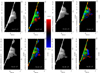 |
Fig. A.1. MSDP Dopplergrams for different times: intensity and Doppler shifts at Hα ± 0.3 Å. Blue and red represent blueshift and redshift, respectively. Yellow and green represent the intensity. The title on the left of each image indicates the local time (CET) in Meudon. The UT time is indicated in the intensity and Doppler-shift maps. |
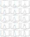 |
Fig. A.2. IRIS Mg II line profiles along slit x = 24 arcsec (slit = 12) crossing the prominence at 16:34:10 UT at 15 selected positions indicated in the panel title and corresponding to pixels along the vertical left line in Fig. 8 (a) and to Table 3 (A1-A15). The unit of the x-axis is Å, the units for intensity are indicated on the left in 104 erg cm−2 s−1 sr−1 Å−1, and on the right in 10−7 erg cm−2 s−1 sr−1 Hz−1. |
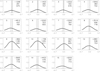 |
Fig. A.3. Example MSDP prominence profiles in the main part at 16:25 UT. Intensities are in 10−6 erg s−1 cm−2 sr−1 Hz−1, and wavelength on the x-axis is in Å. In the right corner, the velocities in m/s at Hα ±0.3 Å are indicated; below, the integrated intensity in erg sr−1 s−1 cm−2 divided by 100 is shown; and on the last row the FWHM in mÅ. In the left corner, the number of the pixel corresponds to points A1-A15 to pixels along the vertical A line in Fig. 2 (a) and in Table 3. |
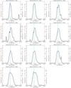 |
Fig. A.4. IRIS Mg II line profiles along slit at x = 46 arcsec crossing the prominence at 16:39:45 UT in 11 selected positions indicated in the panel title and corresponding to pixels along the vertical right line in Fig. 8 (a) and to Table 3 (B1-B11). The unit of the x-axis is Å, and the units for intensity are indicated on the left in 104 erg cm−2 s−1 sr−1 Å−1 and on the right in 10−7 erg cm−2 s−1 sr−1 Hz−1. |
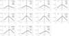 |
Fig. A.5. Example MSDP prominence profiles at the top at 16:25 UT. Intensities are in 10−6 erg s−1 cm−2 sr−1 Hz−1, and the unit of the x-axis is in Å. In the right corner, we see the velocity in m/s at Hα ±0.3 Å; below, the integrated intensity in erg sr−1 s−1 cm−2 divided by 100 is indicated; and on the last row the FWHM in mÅ. In the left corner, the number of the pixel at the top corresponds to points B1-B11 in pixels along the vertical B line in Fig. 2 (a) and in Table 3. |
All Tables
Characteristics of Mg II k and h line profiles of IRIS raster 8 (slit 12 at 16:34:10 UT and slit 23 at 16:39:55 UT) and simultaneous Hα line profiles obtained with the MSDP.
Plasma parameters of the prominence in raster 8 from non-LTE radiative transfer models.
All Figures
|
Fig. 1. Prominence observed by IRIS and the MSDP at the south-west limb of the Sun on 2018 April 19. The panels show (a) a slit-jaw image of the Mg II line (SJI 2796), (b) Hα intensity in the line centre observed by MSDP showing the solar disc used to co-align MSDP and IRIS maps, and (c) Hα ± 0.3 Å intensity observed by MSDP. The dashed lines in panel a mark the field of view of the IRIS raster. |
| In the text | |
|
Fig. 2. Prominence diagnostic based on the MSDP observation. (a) Hα intensity at the line centre, (b) Doppler velocity, and (c) FWHM. The contours present the Hα prominence defined as Mask-Hα (see Sect. 4.7). The blue vertical lines in panel a are the two selected slit positions (A, B) used to analyse the profiles (Figs. A.3 and A.5) and for plasma parameter diagnostics (Table 3). The small horizontal lines are the positions corresponding to profiles A1–A15 and B1–B11. |
| In the text | |
|
Fig. 3. Spatio-temporal evolution of the prominence intensity in Mg II slit-jaw 2796 Å images obtained by IRIS between 14:15 UT to 17:53 UT. The dashed vertical lines mark the IRIS raster field of view. The blue box in panel d defines the FOV used for detailed study of the velocity distribution (Fig. 9). The temporal evolution is available as an online movie (Movie1). |
| In the text | |
|
Fig. 4. Spatio-temporal evolution of the AIA 304 Å intensity observed between 14:15 UT and 17:53 UT. The vertical dashed lines mark the IRIS raster field of view. The overlaid contour corresponds to the contour of the IRIS SJI 2796, level = 1. The temporal evolution is available as an online movie (Movie2). |
| In the text | |
|
Fig. 5. Spatio-temporal evolution of the AIA 171 Å intensity observed between 14:15 UT and 17:53 UT. The vertical dashed lines mark the IRIS raster field of view. We note the presence of the cavity and long extended bright loop in (a), and a bright point in (b). The cavity is visible in all the panels, and the dark twisted column is surrounded with emission. The temporal evolution is available as an online movie (Movie3). |
| In the text | |
|
Fig. 6. Spatio-temporal evolution of the AIA 193 Å intensity observed between 14:15 UT and 17:53 UT. The vertical dashed lines mark the IRIS raster field of view. The overlaid contour corresponds to the contour of the IRIS SJI 2796, level = 1. The dark features (columns and fuzzy dark material) observed in the prominence correspond to the prominence observed in Hα. The temporal evolution is available as an online movie (Movie4). |
| In the text | |
|
Fig. 7. Prominence spectra of raster 8. First row, left panel: reconstructed map using the integrated intensity of Mg II k line, five following panels: spectra along the slit in positions 10 to 14, second row: in positions 15 to 20, and bottom row: in positions 21 to 26. Upper left panel: the dot-dashed vertical lines represent the extreme slit positions (10 and 26) for which the spectra are shown in this figure. The dotted vertical lines are the two selected slit positions used to analyse the profiles and for plasma parameter diagnostics. In panels of the spectra, the vertical dashed blue line corresponds to the rest velocity. In the panel at 16:34:10 UT (slit position 12), the horizontal lines are the positions corresponding to profiles A1–A15 drawn in Fig. A.2. In the panel at 16:39:55 UT (slit position 23), the horizontal lines limit the domain where the profiles (B1–B11) are shown in Fig. A.4. The y-axis is in pixel units (1 pixel = 0.33 arcsec). |
| In the text | |
|
Fig. 8. Prominence reconstructed maps based on the IRIS spectra of Mg II k line (raster 8). (a) Integrated intensity of Mg II k line, (b) Doppler velocity, and (c) width (FWHM) of Mg II k line profile obtained by fitting the profiles with a single Gaussian function. The inner contour line (around x = 10 arcsec) corresponds to the solar surface defined as the level 0.6 Å of the FWHM of Mg II k line; the outer contour corresponds to Mask-Hα based on MSDP observations (see Mask-Hα in Fig. 2). This new contour defined by Mask-Hα (pixels on the disk) is used for the statistics of Mg II parameters in and out the Hα prominence (see Sect. 4.7). The blue dotted lines in panel a are the two selected slit positions (A, B) used to analyse the profiles (Figs. A.3 and A.5) and for plasma parameter diagnostics (Table 3). |
| In the text | |
|
Fig. 9. Histograms of Doppler velocities for Hα and Mg II k lines inside the Hα prominence (left top panel) and in the whole Mg II prominence (right top panel), FWHM for Mg II k line and asymmetry of the Mg II k line computed with the quantile method. Hα prominence corresponds to pixels enclosed by the contour in Fig. 2 panel a and y-range from 60 to 137 arcsec. The whole Mg II k prominence is enclosed in the blue box presented in Fig. 3. The histograms are based only on the spectral profiles with an intensity larger than the noise. |
| In the text | |
|
Fig. 10. Sample of integrated intensity maps in Mg II k line, each map being reconstructed from the 32 spectra of one raster, showing the evolution of the tornado at the top and the long loops connecting with the limb between 14:15 UT and 18:41 UT (rasters 1, 5, 7, 8, 9, 10, 13, and 17). |
| In the text | |
|
Fig. 11. Doppler velocity maps (Gaussian fitting) in Mg II k line computed from the spectra of the rasters observed by IRIS between 14:15 UT to 18:41 UT (rasters 1, 5, 7, 8, 9, 10, 13, 17). The temporal evolution is available as an online movie (Movie5). |
| In the text | |
|
Fig. 12. Probability density functions (PDFs) for Mg II k line parameters for the area between the limb and the outer edge of the Hα prominence contour, y-range from 60 to 137 arc in Fig. 8: (a) intensity versus FWHM, (b) Doppler velocity versus FWHM; outside of the Hα contour, (c) intensity versus FWHM, (d) Doppler velocity versus FWHM; PDFs for Hα line parameters, (e) intensity versus FWHM, and (f) Doppler velocity versus FWHM. The PDF values are plotted in linear scale. |
| In the text | |
|
Fig. 13. (a) Reconstructed filament with flux rope field lines (red lines) overlaid by arcades (green lines). These field lines are obtained from an LMHD extrapolation of an observed photospheric magnetogram for a different prominence. (b) Dips in the magnetic field lines (green lines; adapted from Aulanier & Schmieder 2002). Bottom panels: magnified view of the tornado-like structure showing an accumulation of fine horizontal structures, similarly to the green lines in (b). |
| In the text | |
|
Fig. 14. Prominence body characteristics: (top panelsfrom left to right) Mg II k observed integrated intensity, Doppler shift, and FWHM along slit 12; (bottom panels from left to right) non-LTE model results along slit 12, mean electron density, τ(Mg II k), and τ(H α). The grey areas correspond to pixels where the observed profiles in Mg II cannot be correctly fitted with the grid of profiles derived by the non-LTE radiative transfer code. The red arrows indicate the points in Table 4. |
| In the text | |
|
Fig. 15. Prominence tornado characteristics: (top panels from left to right) observed integrated intensity, Doppler shift, and FWHM along slit 12; (bottom panels from left to right) non-LTE model results along slit 12, mean electron density, τ(Mg II k), and τ(H α). The grey areas correspond to pixels where the observed profiles in Mg II cannot be correctly fitted with the grid of profiles derived by the non-LTE radiative transfer code. The red arrows indicate the points in Table 4. |
| In the text | |
|
Fig. 16. Models of radiative transfer for two parameters: temperature between 6000 K and 20 000 K, and geometrical thickness between 1000 km and 5000 km. Top panel: correlation between integrated intensity of Mg II k versus Hα. The black stars represent the observations (see Table 3). Middle panel: correlation between integrated intensity and EM for Mg II k. Bottom panel: correlation between integrated intensity and EM for Hα. The horizontal lines correspond to the extreme values measured in the prominence body (blue), at the edge (green), and at the top (orange). |
| In the text | |
|
Fig. 17. Theoretical results of the non-LTE radiative transfer code using the fitting profile method. Left panel: pixels where the fitting is satisfactory; middle panel: electron density map; right panel: intensity in Hα according to the models. |
| In the text | |
|
Fig. 18. Ratio relationship between the Mg II h and k integrated intensities computed by the models versus the observations (data). |
| In the text | |
|
Fig. A.1. MSDP Dopplergrams for different times: intensity and Doppler shifts at Hα ± 0.3 Å. Blue and red represent blueshift and redshift, respectively. Yellow and green represent the intensity. The title on the left of each image indicates the local time (CET) in Meudon. The UT time is indicated in the intensity and Doppler-shift maps. |
| In the text | |
|
Fig. A.2. IRIS Mg II line profiles along slit x = 24 arcsec (slit = 12) crossing the prominence at 16:34:10 UT at 15 selected positions indicated in the panel title and corresponding to pixels along the vertical left line in Fig. 8 (a) and to Table 3 (A1-A15). The unit of the x-axis is Å, the units for intensity are indicated on the left in 104 erg cm−2 s−1 sr−1 Å−1, and on the right in 10−7 erg cm−2 s−1 sr−1 Hz−1. |
| In the text | |
|
Fig. A.3. Example MSDP prominence profiles in the main part at 16:25 UT. Intensities are in 10−6 erg s−1 cm−2 sr−1 Hz−1, and wavelength on the x-axis is in Å. In the right corner, the velocities in m/s at Hα ±0.3 Å are indicated; below, the integrated intensity in erg sr−1 s−1 cm−2 divided by 100 is shown; and on the last row the FWHM in mÅ. In the left corner, the number of the pixel corresponds to points A1-A15 to pixels along the vertical A line in Fig. 2 (a) and in Table 3. |
| In the text | |
|
Fig. A.4. IRIS Mg II line profiles along slit at x = 46 arcsec crossing the prominence at 16:39:45 UT in 11 selected positions indicated in the panel title and corresponding to pixels along the vertical right line in Fig. 8 (a) and to Table 3 (B1-B11). The unit of the x-axis is Å, and the units for intensity are indicated on the left in 104 erg cm−2 s−1 sr−1 Å−1 and on the right in 10−7 erg cm−2 s−1 sr−1 Hz−1. |
| In the text | |
|
Fig. A.5. Example MSDP prominence profiles at the top at 16:25 UT. Intensities are in 10−6 erg s−1 cm−2 sr−1 Hz−1, and the unit of the x-axis is in Å. In the right corner, we see the velocity in m/s at Hα ±0.3 Å; below, the integrated intensity in erg sr−1 s−1 cm−2 divided by 100 is indicated; and on the last row the FWHM in mÅ. In the left corner, the number of the pixel at the top corresponds to points B1-B11 in pixels along the vertical B line in Fig. 2 (a) and in Table 3. |
| In the text | |
Current usage metrics show cumulative count of Article Views (full-text article views including HTML views, PDF and ePub downloads, according to the available data) and Abstracts Views on Vision4Press platform.
Data correspond to usage on the plateform after 2015. The current usage metrics is available 48-96 hours after online publication and is updated daily on week days.
Initial download of the metrics may take a while.