| Issue |
A&A
Volume 653, September 2021
|
|
|---|---|---|
| Article Number | A108 | |
| Number of page(s) | 22 | |
| Section | Interstellar and circumstellar matter | |
| DOI | https://doi.org/10.1051/0004-6361/202140824 | |
| Published online | 16 September 2021 | |
Globules and pillars in Cygnus X
III. Herschel and upGREAT/SOFIA far-infrared spectroscopy of the globule IRAS 20319+3958 in Cygnus X★
1
I. Physik. Institut, University of Cologne,
Zülpicher Str. 77,
50937
Cologne,
Germany
e-mail: This email address is being protected from spambots. You need JavaScript enabled to view it.
2
RAL Space, STFC Rutherford Appleton Laboratory,
Chilton, Didcot,
Oxfordshire,
OX11 0QX,
UK
3
ESO,
Karl Schwarzschild Str. 2,
85748
Garching,
Germany
4
Nordic Optical Telescope,
Rambla José Ana Fernández Pérez 7,
38711
Breña Baja,
Spain
5
Department of Physics and Astronomy, Aarhus University,
Ny Munkegade 120,
8000
Aarhus C,
Denmark
6
Department of Physics and Astronomy, West Virginia University,
Morgantown,
WV
26506,
USA
7
Laboratoire d’Astrophysique de Bordeaux, Université de Bordeaux, CNRS,
B18N, allée G. Saint-Hilaire,
33615
Pessac,
France
8
Max-Planck Institut für Radioastronomie,
Auf dem Hügel 69,
53121
Bonn,
Germany
9
Department of Physics and Astronomy, The Open University,
Walton Hall,
Milton Keynes,
MK7 6AA,
UK
10
SOFIA-USRA, NASA Ames Research Center,
MS 232-12,
Moffett Field,
CA
94035,
USA
11
DLR,
Rutherfordstraße 2,
12489
Berlin-Adlershof,
Germany
Received:
17
March
2021
Accepted:
13
August
2021
Abstract
IRAS 20319+3958 in Cygnus X South is a rare example of a free-floating globule (mass ~240 M⊙, length ~1.5 pc) with an internal H II region created by the stellar feedback of embedded intermediate-mass stars, in particular, one Herbig Be star. In Schneider et al. 2012, (A&A, 542, L18) and Djupvik et al. 2017, (A&A, 599, A37), we proposed that the emission of the far-infrared (FIR) lines of [C II] at 158 μm and [O I] at 145 μm in the globule head are mostly due to an internal photodissociation region (PDR). Here, we present a Herschel/HIFI [C II] 158 μm map of the whole globule and a large set of other FIR lines (mid-to high-J CO lines observed with Herschel/PACS and SPIRE, the [O I] 63 μm line and the 12CO 16→15 line observed with upGREAT on SOFIA), covering the globule head and partly a position in the tail. The [C II] map revealed that the whole globule is probably rotating. Highly collimated, high-velocity [C II] emission is detected close to the Herbig Be star. We performed a PDR analysis using the KOSMA-τ PDR code for one position in the head and one in the tail. The observed FIR lines in the head can be reproduced with a two-component model: an extended, non-clumpy outer PDR shell and a clumpy, dense, and thin inner PDR layer, representing the interface between the H II region cavity and the external PDR. The modelled internal UV field of ~2500 G° is similar to what we obtained from the Herschel FIR fluxes, but lower than what we estimated from the census of the embedded stars. External illumination from the ~30 pc distant Cyg OB2 cluster, producing an UV field of ~150–600 G° as an upper limit, is responsible for most of the [C II] emission. For the tail, we modelled the emission with a non-clumpy component, exposed to a UV-field of around 140 G°.
Key words: ISM: atoms / ISM: clouds / HII regions / photon-dominated region / ISM: molecules / ISM: kinematics and dynamics
The [C II] data shown in Figs. 4 and 5 (FITS files) are only available at the CDS via anonymous ftp to cdsarc.u-strasbg.fr (130.79.128.5) or via http://cdsarc.u-strasbg.fr/viz-bin/cat/J/A+A/653/A108
© ESO 2021
1 Introduction
In the vicinity of massive stars, intriguing structures such as column-shaped pillars and cometary-shaped globules are frequently detected in optical as well as near- and far-infrared images (e.g. Schneps et al. 1980; Hester et al. 1996; White et al. 1997; Schneider et al. 2016). They are mostly the result of feedback processes – ionisation and stellar winds – from massive stars and point toward the illuminating source. Larger pillars, however, can also reflect the primordial cloud structure (White et al. 1999; Lefloch et al. 2008; Miao et al. 2009) or arise from eroded convergent flows (Dale et al. 2015). Pillars still have a physical connection to the gas reservoir of the molecular cloud, while globules are isolated features. Figure 1 shows an example for such objects in the Cygnus X region (Schneider et al. 2016).
External UV-radiation creates photodissociation regions (PDRs) on the surfaces of pillars and globules, often visible as a bright rim, facing the ionising source. A rare example of a globule suggested to be also illuminated internally by massive stars is IRAS 20319+3958 in Cygnus X (Schneider et al. 2012, 2016; Djupvik et al. 2017). This source (hereafter, ‘the globule’) is explored in this paper. Other examples of star-formation activity within globules are found in Comerón & Torra (1999). The globule is also impacted by the radiation of the Cyg OB2 cluster located at a projected distance of ~30 pc from the globule, assuming that this cluster is located at a distance of 1.4 kpc. It is notoriously difficult to derive distances in Cygnus X, see Schneider et al. (2006); Comerón et al. (2020) for more detailed discussions. We use the value of 1.4 kpc, which is based on maser observations (Rygl et al. 2012) of prominent star-forming sites in Cygnus X. An analysis of Gaia data (Lim et al. 2020) of Cyg OB2, however, arrived at a larger distance of 1.6 kpc.
Many details of the formation and evolution of globules and pillars have not yet been settled. Numerical modelling started out with simple models of photo-ionisation (e.g. Lefloch et al. 1994) that explained basic properties such as shapes or lifetimes (Johnstone et al. 1998), while the concept of radiative-driven implosion (Bertoldi 1989) provides an explanation of how stars can form in pillars and globules. More realistic models with a careful treatment of heating and cooling processes (e.g. Miao et al. 2006) that consider the turbulent structure of the gas (Gritschneder et al. 2009) and the curvature of the cloud surface (Tremblin et al. 2012a,b) now have the capacity to explain additional properties, such as the velocity field of the observed features. Furthermore, new observations, including Herschel imaging and spectroscopy in the far-infrared (FIR) and SOFIA (Stratospheric Observatory for Far-Infrared Astronomy) FIR spectroscopy, make it possible to establish a classification scheme and a possible evolutionary sequence. In the first part of this series of papers (Schneider et al. 2016), we set up a categorisation based on Herschel 70 μm photometry and we propose that pillars advance into globules, which, in turn, evolve into evaporating gaseous globules (EGGs), dense gas condensations without star-formation, or objects with protoplanetary disks (proplyds); or they only resemble proplyds (proplyd-like), depending on density and incident UV-field. In the second paper (Djupvik et al. 2017), we carried out optical and near-IR imaging and spectroscopy of the globule in order to obtain a census of its stellar content and the nature of its embedded sources.
In this work, we present spectroscopic observations of FIR cooling lines of the globule in the southern part of Cygnus X (Reipurth & Schneider 2008), where the very massive and rich Cyg OB2 association illuminates the molecular cloud. The globule was mapped in the [C II] line with SOFIA (Schneider et al. 2012) as well as with Herschel/HIFI, PACS, and SPIRE (thispaper). It was covered in Herschel imaging observations of Cygnus X within the Herschel imaging survey of OB Young Stellar objects (HOBYS, Motte et al. 2010) and was also shown and discussed in Schneider et al. (2016). Figure 1 displays a three-colour image of the Herschel photometry data with our source indicated.
The objective of this paper is to study the spatial emission distribution of various PDR tracers and to perform a careful analysis of line intensities and ratios using the KOSMA-τ PDR model (Röllig et al. 2006) to disentangle external (Cyg OB2) and internal excitation sources. We intend to show that it is possible to explain most of the observed lines in a PDR model considering the geometry of the source. This approach is more sophisticated than studies that assume plane-parallel, homogeneous layers of gas. There are not many sources holding such a large data set of cooling lines in the mm- to FIR. All the line intensities are given in the accompanying tables and the maps can be provided on demand (the HIFI [C II] data is already provided via CDS, see Sect. 2.1), offering the possibility for other applications and studies.
Another goal is to study the dynamics of the globule. The velocity-resolved extended [C II] map suggests that the globule rotates and that high-velocity outflowing gas escapes from the globule head (some features were shown in Schneider et al. 2012, but not in such detail).
We present the various data sets (Herschel, SOFIA, FCRAO, JCMT) in Sect. 2, including a consistency check between FIR line intensities observed with Herschel and SOFIA. We give an overview of what is already known about the globule in Sect. 3. In Sect. 4, we present the so far unpublished [C II] HIFI and [O I] upGREAT maps of the globule. Section 5 provides details about the PDR modelling and discusses the PDR properties of the globule. Section 6 presents our summary.
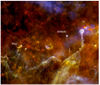 |
Fig. 1 Three-colour (blue: 70 μm, green: 160 μm, red: 250 μm) image (Schneider et al. 2016) of the environment of Cyg OB2 with the globule IRAS 20319+3958, labeled as ‘globule’. The size of the image is ~1.5° × 1.4°, which corresponds to ~36 pc × 34 pc, assuming a distance of 1.4 kpc. The pillar indicated further east will be presented in another study. The most massive stars of the Cyg OB2 association are located in the northwest corner of the image (north is up, east to the left). |
2 Observations
2.1 Herschel spectroscopy
Far-infrared spectroscopic observations of the globule were performed with the Herschel Space Observatory (Pilbratt et al. 2010), using the instruments HIFI (de Graauw et al. 2010), PACS (Poglitsch et al. 2010), and SPIRE (Griffin et al. 2010) within the framework of the Herschel Open Time priority 1 project (ot1_nschneid_1) Pillars of creation: physical origin and connection to star formation (PI: N. Schneider). Table 1 summarises the observational parameters, such as observation date, central position, and map size. All the data is available in the Herschel science archive. For convenience, we provide the HIFI [C II] data cube and line integrated intensity at the Centre de données astronomiques de Strasbourg (CDS).
2.1.1 HIFI
The HIFI data consist of Nyquist-sampled, position switched on-the-fly (OTF) maps of the [C II] line at 158 μm with a beam size of 12.2′′ in band 7b at 1910 GHz. We employed the wide-band spectrometer (WBS) with an local oscillator (LO) frequency of 1897.662 GHz. The WBS has a full intermediate frequency (IF) bandwidth of 4 GHz at a spectral resolution of 1.1 MHz (corresponding to a velocity resolution of 0.7 km s−1), in both horizontal (H) and vertical (V) polarisations. The frequency range covered in band 7b is 1892.6–1895.2 GHz in the lower sideband (LSB) and 1899.9–1902.5 GHz in the upper sideband (USB). The Herschel Interactive Processing Environment, (HIPE) version 8.2 was used to remove standing waves and to convert the observed data to CLASS fits-format and the GILDAS packages1 were used for all further procedures (baseline subtractions, line fittings etc.). In order to obtain a better signal-to-noise ratio (S/N), we averaged the H and V polarisations. The final processed Level 2 data is scaled in  . To scale our data to Tmb we multiplied
  by the factor of ηl∕ηmb where ηl is the forward efficiency (0.96) and ηmb is the main beam efficiency (0.69) in band 7b. The overall calibration accuracy is ~10% (Roelfsema et al. 2012).
Summary of the HIFI, PACS, and SPIRE spectroscopic observations.
2.1.2 PACS
For the PACS range spectroscopy of the globule head, we used the integral field spectrometer to investigate important cooling lines, namely, the [O I] 63 and 145 μm lines, the [N II] 122 μm line, and high-J CO lines. The data were observed in two wavelength ranges: from 51 to 73 μm (blue side) and from 110 to 208 μm (red side). The pipeline processes and all data reduction steps (baseline subtraction, line fitting etc.) were done with HIPE version 7.0 via the built-in pipeline scripts. The line flux measurements were done as described in Schneider et al. (2012), using the PACSman software (Lebouteiller et al. 2012). We note that because the PACS maps are contaminated by emission in the off-position, the calibration was derived only from on-source data and thus associated with a larger error (~30%). For more details, see also Sect. 2.6, where we compare several FIR lines that were observed with Herschel and SOFIA. The PACS maps of the globule head are displayed in Fig. A.1.
2.1.3 SPIRE
The spectra were taken with the SPIRE Fourier Transform Spectrometer (FTS) long and short wavelength receivers (SLW and SSW, respectively) at two positions with sparse sampling. One position is located in the globule head and one in the tail (see Table 1). The SLW observes a hexagonal pattern of 19 spectral pixels (spaxels) covering the wavelength range 313–671 μm and the SWS observes 37 spaxels covering 194–312 μm. The beam size at the receiver’s central spaxels varies between 16″–20″ for SSW and 31″–43″ for SLW.
The SPIRE-FTS data were downloaded from the Herschel Science Archive, processed using HIPE v14.1, with SPIRE calibration files spire_cal_14_3. The FTS extended source calibration (Swinyard et al. 2014) was used, and in HIPE v14.1, this includes the updates described in Valtchanov et al. (2018) to align the absolute brightness level to match the SPIRE photometer.
The lines were fitted using the Spectrometer Cube Fitting script in HIPE v15, which carries out a simultaneous fit of the spectral lines and continuum in each band for every spaxel in the spectral cube. The SPIRE maps of the globule head and tail are displayed in Figs. A.1 and A.2.
2.2 Herschel imaging
We used Herschel imaging observation of PACS at 70 and 160 μm, and SPIRE at 250, 350, and 500 μm obtained within the HOBYS guaranteed time Key Program (Motte et al. 2010). The angular resolution of the data varies between 6″ and 36″ (see Table 2). Column density and dust temperature maps, both at an angular resolution of 36″, were produced with a pixel-by-pixel SED fit to the wavelengths 160–500 μm as described in Schneider et al. (2016).
2.3 SOFIA
2.3.1 GREAT: [C II] 158 μm and CO 11→10
The [C II] 1.9 THz line and the CO J = 11→10 molecular rotation line at 1.267 THz were observed with the PI-heterodyne receiver GREAT2 (Heyminck et al. 2012) on SOFIA during one flight on November 10, 2011 from Palmdale, California. OTF maps of the globule, with an angular resolution of ~15″ for [C II] and 23″ for CO, were produced. This data set was presented in Schneider et al. (2012). In this paper, we compare the SOFIA [C II] data with what was obtained with HIFI and use the line intensity information of the CO J = 11→10 line for PDR modelling.
2.3.2 upGREAT: [O I] 63 μm and CO 16→15
The globule was observed on November 2, 2016, during one flight from Palmdale, California with upGREAT (Risacher et al. 2016) on SOFIA. Only the globule head was covered (map size ~100″ × 80″), the central position was RA(2000) = 20h33m53.0s, Dec(2000) = 40°08′45″. The seven-pixel HFA array was tuned on the [O I] 4.7 THz line, the single pixel L2 channel was tuned on the CO 16→15 line. Both channels observed in parallel, optimised for the [O I] line. We note that the observed CO 16→15 map thus has missing data points because of the single pixel sampling. The observing mode was chopping single phase A, with a chop amplitude of 100″ and a chop frequency of 0.655 Hz with one cycle per dump. The OTF mapping was performed with 1 slew per ref and 6 refs/load. The array orientation was –19.1°. The bandpass averaged system temperature was 2657 K for the L2 channel and 3512 K for the H-array. All line intensities are reported as main beam temperatures scaled with main-beam effciencies of 0.69 and 0.68 for [O I] and CO, respectively, and a forward effciency of 0.97. The main beam sizes are 15.3″ for the L2 channel (12CO 16→15) and 6.1″ for the HFA channel ([O I],).
Summary of the observational data sets of the globule.
Comparison of line integrated intensities.
2.4 FCRAO data
We used molecular line data obtained with the 14 m dish of the Five College Radio Astronomy observatory (FCRAO), employing the single sideband focal plane array receiver Second Quabbin Optical Imaging Array (SEQUOIA). The whole Cygnus X region (~35 square degrees) was observed in the 13CO 1→0 at 110.201 GHz, the C18O 1→0 at 109.782 GHz, and the CS line at 98.0 GHz. The beamwidth of the FCRAO at 110 GHz is 46″. More detailsare found in Schneider et al. (2011), where the CO data sets are presented.
2.5 JCMT CO data
The 12CO 3→2 data used in this paper were obtained with the 16-pixel array HARP receiver in the B-band, and the ACSIS digital autocorrelation spectrometer as the backend correlator system. The individual beams of HARP have a full width at half maximum (FWHM) of 15″ and the beams are spaced 30″ apart on a 4 × 4 grid. The map of the globule is part of the programs M07BU019 (PI: R. Simon) and M08AU018 (PI: N. Schneider) that were carried out in 2007 and 2008 to map large parts of Cygnus X North and South. The data have a velocity channel spacing of 0.42 km s−1.
2.6 Consistency check between FIR lines observed with PACS, SPIRE, and HIFI (Herschel) and (up)GREAT (SOFIA)
The globule is a rare example of a source that was observed in various FIR lines with different instruments on Herschel and SOFIA over the last seven years and thus offers the possibility to compare the observed line intensities. The estimated total calibration uncertainties are ~20% for GREAT and upGREAT (Heyminck et al. 2012; Risacher et al. 2016), and 10% for HIFI (Roelfsema et al. 2012). The SPIRE calibration uncertainty for extended sources was estimated to be 7% (Swinyard et al. 2014), although when there is structure in the beam, the uncertainty is larger and dominated by source-beam coupling (Wu et al. 2013). Our data include the latest corrections to match the FTS extended calibration to the SPIRE Photometer (Valtchanov et al. 2018). The PACS data suffer from contamination in the off-position so that the calibration was done only using the on-source data. We thus estimate that the error on the flux is high (>30%) and the observed values are upper limits.
Table 3 shows a comparison between the [C II] 158 μm line, the [O I] 63 μm line, and the CO 11→10 μm lines, determined at one position in the globule head at RA(2000) = 20h33m49s, Dec(2000) = 40°8′45″. The flux values obtained for [C II] for HIFI and GREAT as well as the CO 11→10 line for SPIRE and GREAT agree very well. In contrast, the PACS values for the [C II] and the [O I] line are significantlylower than those obtained with HIFI/GREAT and upGREAT, respectively, which cannot be explained by the PACS contamination problem in the off-position because the PACS values are upper limits. One explanation can be attributed to positional uncertainties because the [O I] line emission show a large spatial pixel-to-pixel variation and pointing differences can lead to different values. We take the SOFIA [O I] 63 μm data for PDR modelling, but we need to use the PACS [O I] 145 μm data since this line was only observed with Herschel. However, this caveat needs to be kept in mind.
Physical properties of the globule in total (Col. 2) and the head and tail (Cols. 3 and 4), respectively.
3 Multiwavelengths observations of the globule
In the following, we shortly present previous works on the globule and summarise the most important physical properties in Table 4.
IR- and FIR-data
Figure 2 displays the globule in the IR- to FIR-wavelength range (3.6–500 μm, observed with Spitzer and Herschel), and in the molecular lines of CS 2→1 and 12CO 3→2. The IR data show the stellar content of the globule and its environment, while the FIR observations at 70 and 160 μm have a too low angular resolution (6″ and 11″, respectively) to resolve the (proto)-stars. The head and tail are well visible at all wavelengths, indicating that there is warm and cold dust present in both. The IR traces the hot PAH dust features while the FIR data longer than 160 μm trace the warm to cold dust. The tail/head ratio flux peaks around 160 μm, but the globule head clearly dominates the emission at all wavelengths. We note that the tail contains no pre- or protostellar sources.
Molecular line data
The two lower right panels of Fig. 2 show that the line-integrated 12CO 3→2 and CS 2–1 emission arises from the whole globule though the peak of emission is found in the head. The CS emission is more beam diluted because of the lower resolution of46″ with respect to CO 3→2 with 15″. Intererestingly, there is a lack of CO 3→2 emission in the northeastern globule head, giving the impression that gas was blown out of the centre, leaving this hole. The density of the globule is at least ~104 cm−3 if we assume that the molecular line emission is thermalised (Shirley 2015).
Herschel column density and temperature maps and the UV field
High (column) densities are confirmed by the Herschel dust column density map (Fig. 3, left panel), which indicates peak values of a few 1022 cm−2 for the globule head, (see also Schneider et al. 2016), where the column density map, temperature map, and UV-field map were already shown for a larger area and the globule was labelled ‘g1’ in region 1–3. The values for average H2 column density ⟨N⟩, mass M, average density n, length and width, and dust temperature T are given in Table 4. We note that we averaged across the whole head as it was originally defined (Schneider et al. 2016) by 70 μm emission, which corresponds to the area seen in the temperature map. The average values for column density and density are thus lower than as if we would have only taken the high column density area seen in Fig. 3. The temperature, also determined from an SED fit to the Herschel data, is 19.7 K, but shows a strong variation from 17.2 K south of the globule centre to 26.3 K at the centre of the globule head (Fig. 3, middle panel).
From the Herschel 70 and 160 μm flux, Schneider et al. (2016) calculated an average UV flux across the globule head of ~550 G° (in units of the Habing field3) and a peak value (in a 20″ beam) of ~4300 G°. From a census of the exciting stars of the Cyg OB2 cluster, the incident UV-field on the globule is only 150–600 G° (not accounting for extinction by the molecular clouds of the Cygnus X region and ignoring projection effects). We thus anticipate that internal sources must also contribute to the measured UV field from the Herschel fluxes.
Stellar content inside the globule
Earlier studies reported nine cluster members within a projected radius of ~0.5 pc (Kronberger et al. 2006; Kumar et al. 2006) and two visible stars had been estimated to have mid-B spectral types (Cohen et al. 1989). The scenario of embedded stars was further explored in Djupvik et al. (2017), where we found that the globule contains an embedded aggregate of about 30–40 young stellar objects within one arcmin (or 0.4 pc with the adopted distance of 1.4 kpc). Based on the high ratio of Class I to Class II objects, the small cluster was estimated to have an age <1 Myr. The most massive members were designated stars A, B, and C. Star A was discovered to be a binary with one component being a Herbig Be star with an estimated mass of 13 M⊙. Star B was found to have spectral type B0.5 to B1.5 and an estimated mass of 23 M⊙. The bright mid-IR Class I source, Star C, was resolved in a binary, of which at least one is a massive YSO of spectral type late O or early B with 8.1 M⊙. Optical spectroscopy of the nebula next to these stars revealed clear signs of a low-excitation H II region, as one would expect from early B-type stars rather than the harder radiation from O stars in the nearby Cygnus OB2 association. Furthermore, the morphology seen in high-angular-resolution images of H2 line emission tracing the PDR, and Br-γ line emission tracing the ionised gas, was interpreted as additional evidence that the globule is illuminated from the inside.
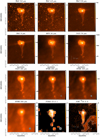 |
Fig. 2 Globule at IR- and FIR-wavelengths: Spitzer/IRAC 3.6–8 μm, Spitzer/MIPS at 24 μm, Herschel/PACS 70, and 160 μm and SPIRE 250, 350, and 500 μm (all units areMJy sr−1). The two lower right panels show velocity integrated molecular line emission of CS 2→1 and 12CO 3→2 in [K km s−1]. The beam is indicated in all panels with longer wavelength observations (starting with PACS 160 μm) in the lowerright corner. The Spitzer data were already displayed in Djupvik et al. (2017) and the Herschel data in Schneider et al. (2016). |
4 Results and analysis
Here, we present a study of many cooling lines in the mm- to FIR-wavelength range, which all arise from photodissociation regions (PDRs). The hot (T > 100 K) PDR component is best traced in the cooling lines of atomic oxygen ([O I] at 63 and 145 μm) and high-J CO rotational lines. The warm (T ~ 100 K) layer of the PDR is seen in the 158 μm line of ionised carbon, followed by the fine-structure lines of neutral carbon ([C I] 1→0 and 2→1 at 609 and 370 μm, respectively). The cool (T < 50 K) molecular cloud is traced in low-J CO lines. Apart from the gas temperature and UV field, it is also the density in the PDR that determines which of the lines is the dominant cooling line. It is a major challenge to correctly reproduce the observed line intensities in PDR models. Some models focus on establishing a careful chemical network, while others emphasise geometrical effects, such as considering the inhomogeneous structure of the PDR (e.g., Tielens & Hollenbach 1985; Black & van Dishoeck 1987; Le Bourlot et al. 1993; Kaufman et al. 1999; Sternberg & Dalgarno 1995; Wolfire et al. 2003; Meijerink & Spaans 2005; Röllig et al. 2006; Bisbas et al. 2015). Röllig et al. (2007) and Bisbas et al. (2015) give an overview of the various PDR codes with a comprehensive reference list.
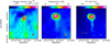 |
Fig. 3 Herschel view of the globule. From left to right: column density (contours 1.3, 1.8, 2.3, 2.8 1022 cm−2), temperature (contours 17.1, 17.5, 19, 21, 23, 25 K), and UV-flux map (contours 150, 200, 500, 1000, 2000 G°) of the globule obtained from Herschel. These images are cut-outs from figures shown in Schneider et al. (2016). The column density and temperature maps have an angular resolution of 36″ and the UV map of 20″. These resolutions are indicated in the lower right corner of each panel. |
4.1 Herschel/HIFI [C II] 158 μm emission distribution
Figures 4 and 5 show the spatial and velocity distribution of the [C II] emission in the globule observed with HIFI on Herschel. The overall emission in the globule head is similar to what was found in Schneider et al. (2012), based on GREAT/SOFIA observations. We note that the globule tail was not observed with SOFIA in 2012. The channel maps (Fig. 5) reveal the correlation between [C II] emission and the stellar content. Star A (the Herbig Be star, black triangle) displays a clear correlation between high velocity [C II] emission in the blue (2.5–5.3 km s−1) and red (11.6–13 km s−1) velocity range. We observe outflowing gas from the inner PDR region around Star A that had already created a small cavitybecause of its stellar wind and radiation (Schneider et al. 2012). This point is discussed in more detail in Sect. 4.4. Interestingly, the two other star systems do not display a strong correlation with [C II] emission. Star B (the single early B-star, white rectangle) lies outside of significant [C II] emission for all velocity channels, while Star C (binary with a late O star, grey cross) can also serve as an exciting source for ionising carbon in the PDR region. The channel maps show that the bulk emission of the globule between ~6.7 km s−1 and 10.2 km s−1 has first a prominent peak enclosing the three stellar systems, then forms an arc-like structure (v = 8.1 km s−1) and then develops a single peak south-east of the stars.
The globule tail is fainter in [C II] emission. The integrated intensity in the tail (Fig. 4) is typically ~10 K km s−1, which is a factor of 10–15 smaller than what is found in the globule head. Nevertheless, this level of [C II] emission indicates that there is some external heating (there are no exciting sources in the tail) from the overall FUV field around the globule, mostly caused by the Cyg OB2 cluster.
4.2 [C II] column density and mass
We calculate the mass associated to the gas traced by [C II] emission using a simplified version of the formula for the [C II] column density in the limit of optically thin emission given by Eq. (2) in Langer et al. (2010) or Eq. (26) in Goldsmith et al. (2012) that is
![Mathematical equation: \begin{equation*}\hskip-1pt N(C^+) = 2.9 \times 10^{15} \, \left(1 + 0.5 \, e^{91.25/T_{\textrm{kin}}} \left(1 + \frac{2.4 \times 10^{-6}}{R_{\textrm{ul}} \, n}\right)\right) \, I(C^+) \, [\textrm{cm}^{-2}],\!\!\!\!\end{equation*}](/articles/aa/full_html/2021/09/aa40824-21/aa40824-21-eq3.png) (1)
(1)
with Rul as the collisional de-excitation rate coefficient at a kinetic temperature Tkin and density n of the collisional partner, which may be either electrons or atomic or molecular hydrogen. In addition, I(C+) is the line integrated observed [C II] intensity. As a first-order approximation, we assume high kinetic temperatures and high densities, so that this equation is simplified to:
![Mathematical equation: \begin{equation*}N(C^+) = 4.38 \times 10^{15} \, I(C^+) [\textrm{cm}^{-2}].\end{equation*}](/articles/aa/full_html/2021/09/aa40824-21/aa40824-21-eq4.png) (2)
(2)
We distinguish between the gas entrained in the outflow in the globule head, namely, [C II] emission in the blue (v = 0–5 km s−1) and red (v = 12–15 km s−1) velocity range, and the bulk emission (v = 5–12 km s−1). For the bulk emission, we derive an average [C II] column density of 2.0 × 1017 cm−2 and 0.4 × 1017 cm−2 for the globule’s head and tail, respectively. Assuming an abundance of C/H = 1.2 × 10⁻⁴ (Wakelam & Herbst 2008), we estimate a mass of ~13.63 M⊙ and ~1.55 M⊙ for the globule head and tail, respectively. The gas mass in the outflow is 1.57 M⊙ and 0.68 M⊙ for the blue and red velocity range, respectively. We note that the masses derived from [C II] are lower limits and lower than what was derived from the dust. However, the values are not directly comparable. While dust emission is optically thin and traces all gas along the line-of-sight, the [C II] emission can be optically thick and arise mostly from the PDR surface.
4.3 Large-scale dynamics of the globule
The dynamics of the globule head was already discussed in Schneider et al. (2012). We confirm with the HIFI [C II] data the detection of a velocity gradient and differences in line position and width within the globule head (cf. Fig. 5). Figure 6 displays position-velocity (PV) plots for five vertical cuts through the whole globule that are indicated in Fig. 4. The cuts at offsets 0 and −10″ cross Star A and we observe – similar to the channel maps – high velocity blue- and red-shifted emission and an opening in the globule head with an arc-like structure. The cuts further away from Star A show more confined emission spatially and kinematically and reflect the primordial velocity structure of the globule with gas around 7 km s−1. The globule tail does not show a velocity gradient along its main axis (north-south orientation) in the individual cuts, but there is an east-west velocity gradient. This becomes obvious in an overlay between the emission in the cuts at −10″ and −30″ (Fig. 7) and is also seen in the channel maps of Fig. 5. The ‘blue’ part of the [C II] tail at 7.4 km s−1 is located further west compared to the ‘red’ part of the [C II] tail visible at higher velocities around 8.1–8.8 km s−1.
Figure 8 displays the velocity pattern of the whole globule in more detail, this time including the tail, which was not observed in [C II] before. The globule head shows a possible rotation feature with an inclined north-south axis, similar what was seen in Schneider et al. (2012). The globule tail also shows a possible rotation, but the axis is less inclined and the velocity difference is smaller. The rotation is clock-wise around an axis located between the blue and red part of the tail if we view the globule from above.
Possible rotation features in pillars were observed before (Gahm et al. 2006; Sofue 2020). Gahm et al. (2006) proposed for ‘elephant trunks’ in several sources observed in CO lines that rotation can be provoked by the formation of compressed magnetic filaments that were present in the parent molecular cloud and are now impacted by the expanding H II region. They developed a double helix model in which a pillar rotates as a solid body with the same angular speed along the major axis. This picture would be consistent with the observations for our globule. In this case, it is possible that the globule started as a pillar (proposed in Schneider et al. 2016), which was linked to the bulk emission of the molecular cloud and had the same velocity. After the pillar detaches from the cloud, it becomes a globule that floats freely into space but still carries the initial momentum of the pillar. Simulations (Tremblin et al. 2012b) predict thatpillars and globules in the same close environment have a velocity difference of typically a few km s−1. This applies also to our globule, as shown in Schneider et al. (2012). Other models of UV radiation impacting a turbulent cloud (Gritschneder et al. 2009) display a slightly different picture. The UV-radiation clears out and pushes away the low-density material of the cloud but leaves dense structures, such as pillars (see their Fig. 1). The extent to which magnetic fields and the impact of the external UV-radiation can also influence the velocity field seen in [C II] is not clear and this area requires further investigation.
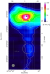 |
Fig. 4 Line-integrated [C II] 158 μm emission of the globule obtained with HIFI on Herschel in the velocity range 0–15 km s−1. The blacktriangle indicates the double system (Star A) of which at least one is a Herbig Be star, the white rectangle points to Star B with a B0.5 - B1.5 spectral type, and the black cross marks Star C, a resolved binary of which one is a late O or early B star. The centre position (0,0) is at RA(2000) = 20h33m49.95, Dec(2000) = 40°07′42.75″. The [C II] beam is indicated in the lower left corner. The dashed lines indicate the vertical (north-south) cuts where we performed position-velocity maps and the dark grey circles mark the positions and the extend of the SPIRE beam for the longest wavelengths (FWHM ~ 40″) we used for PDR modelling. The position in the north is the globule ‘head’ and the one in the south the globule ‘tail’. |
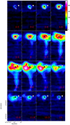 |
Fig. 5 Channel maps of [C II] emisson obtained with HIFI on Herschel from 2.5 to 13 km s−1. The symbols indicate the three stellar systems, similar to Fig. 4, except that here Star C is indicated with a white cross for better visibility. |
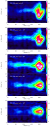 |
Fig. 6 Position-velocity maps of the globule in [C II] for 5 vertical cuts cuts in declination at different RA offsets, indicated in Fig. 4. The zero-offset is at RA(2000) = 20h 33m50s and goes then in steps of 10″. The Dec (2000) range is 40°05′15″ to 40°09′45″. The bottom panel for cut = −40″ outlines with a white dashed rectangle the globule’s tail for which we show an overlay between two PV cuts in Fig. 7. |
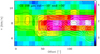 |
Fig. 7 Overlay between PV maps of the globule in [C II] for the −10″ (black contours) and −30″ (white contours) vertical cuts, indicated in Fig. 4. The dashed lines show the centre velocity of the globule’s tail for the cuts, i.e. 8.20 km s−1 for the −10″ cut and 7.35 km s−1 for the −30″ cut, respectively. |
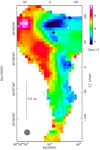 |
Fig. 8 Velocity map (first moment) of the [C II] emission, showing possible patterns of counter-clockwise rotation with the approximate axes indicated with dashed lines. The centre position (0,0) is at RA(2000) = 20h33m49.95, Dec(2000) = 40°07′42.75″. The [C II] beam is indicated in the lower left corner. We note that the axes for the globule head, where most of the mass resides, and the tail have not the same inclinations, and the velocity difference is larger for the head (~9.5 to ~6.9 km s−1) than for the tail (~8.3 to ~7.4 km s−1). The grey contour outlines the 2 K km s−1 contour level of [C II] emission, the symbols are the same as in Fig. 4. |
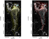 |
Fig. 9 Continuum subtracted narrow-band image that contains the H2 1–0 S(1) ro-vibrational line at 2.122 μm (Djupvik et al. 2017) at ~2″ resolution with contours of velocity-integrated 12CO 3→2 emission (yellow, left panel) and velocity-integrated [C II] emission (red, right panel), both at 15″ resolution, overlaid. The CO contours go from 1 to 13 by 1.5 K km s−1 and the [C II] contours go from 5 to 155 by 15 K km s−1. The embedded stars A, B, and C are indicated. |
4.4 Comparison to H2 emission and small-scale dynamics of [C II] emission
Figure 9 shows how the emission distributions of cool molecular gas (traced by CO) and warm PDR gas (traced by [C II]) compare to the narrow-band imaging of the H2 1–0 S(1) at 2.122 μm. This line is excited either by shocks, driven by stellar winds, but can also be associated with dense PDRs. A large opening towards the north-east becomes obvious in the H2 and CO 3→2 map and suggests that the internal H II region breaks out of the globule. The deficit of molecular gas is also clearly seen in the Herschel column density map in Fig. 3. In contrast, the peak in column density seen in Fig. 3 corresponds also to peak emission in CO and H2, and Star C is centred on this dense clump. Interestingly, the [C II] emission shows no decline in the north-eastern corner of the globule (right panel in Fig. 9) and the emission peak is clearly centred on Star A. In fact, we observe high-velocity blue- and red-shifted emission in [C II], shown in Fig. 10, suggesting an outflow oriented along the line-of-sight of the observer. The outflow is very collimated and could thus originate from a young stellar object (YSO) (the [C II] beam is 15″ so that the emissionis beam diluted). It is unlikely that this very localised outflow interacts with the external UV field. The red wing (velocities >12 km s−1) is fully visible in the [C II] spectra taken around the position of Star A and displayed in Fig. 11. There is no high-velocity emission detected in CO 16→15 and only a very weak velocity component in [O I] 63 μm around 12 km s−1.
In Djupvik et al. (2017), we found that Star A has two components of which one is an early B-type star, a Herbig Be star. These objects are intermediate-mass pre-main-sequence stars and are divided into three categories (Fuente et al. 2002): the youngest (~0.1 Myr) Type I starsare embedded in a dense molecular clump and have associated bipolar outflows that are detected in CO. Type II stars are also associated to molecular material, but not immersed in a dense clump, their ages are between a few 0.1 to a few Myr. Type III stars (typical age >1 Myr) have fully dispersed the surrounding material and created a cavity inside the molecular cloud. In addition, Diaz et al. (1998) showed that only stars with spectral type earlier than B5 can create significant PDRs. Our observations are, thus, fit best with an Herbig Be Type III star since we observe that the star is located in a cavity and not associated with a dense clump, that there isno CO outflow, but high-velocity [C II] emission, tracing the PDR surfaces of the inner cavity walls, namely, the interface between the H II region and the molecular gas. This sort of [C II] dynamics was also observed – and interpreted in a similar way – for the bipolar nebula S106 (Schneider et al. 2018). We note that we exclude shock excitation as a significant origin for the outflow because firstly, [C II] is not a good shock tracer and its origin is mostly PDRs, and secondly, the [O I] 63 μm line does not show prominent high-velocity wings, which would be the case if there were shocks.
It is out of the scope of this paper to go into more detail what is the driving source for the [C II] outflow, but we note that it must be associated with the Herbig Be star. In the literature on Herbig Ae and Be stars, accretion and outflow signatures were detected (Cauley & Johns-Krull 2014; Moura et al. 2020; Rodriguez et al. 2014), and stellar winds are commonly promoted asthe most likely outflow mechanism, although magneto-centrifugally driven outflows from the star–disk interaction region can also occur. Higher angular resolution cm-observations and spectroscopy of lines from the stellar atmosphere of the star may help to investigate in more detail the accretion and outflow properties of the source.
In any case, we confirm the conclusion from Djupvik et al. (2017) that the emission distribution of H2 indicates that the sources of ionisation are the B stars of the embedded aggregate, rather than the external UV field caused by the O-stars of Cyg OB2. We note that another line of evidence in Djupvik et al. (2017) showed that the visible spectrum of the H II region is that of a soft ionising radiation, typical of an early-B star. In Sect. 5.1, we will give further evidence for this proposal by modelling the observed FIR lines.
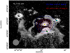 |
Fig. 10 Map of H2 2.12 μm emission (Djupvik et al. 2017) with contours of [C II] outflow emission. The blue velocity range of the [C II] line ranges from 0 to 5 km s−1, contours go from 10 to 50 by 10 K km s−1. The red velocity range is 12–15 km s−1 and contoursgo from 3 to 13 by 2 K km s−1. The embedded stars and the [C II] beam size are indicated. |
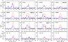 |
Fig. 11 Spectral maps of the [O I] 63 μm line (blue), the [C II] 158 μm line (red) and the CO 16→15 line (black) of the globule head in the velocity range −5 to 20 km s−1. The leftmostmain beam brightness temperature scale ranges from −0.2 to 2 K and is valid for [O I] and CO 16→15. The temperature scales at each panel are valid for [C II]. All data are smoothed to an angular resolution of 20″ and sampledon a grid of 20″ in order to increase the S/N. However, the CO 16→15 line was not observed at all positions (Sect. 2) so that we only plot the few spectra with observed emission above the 5σ level. The velocity resolution is 0.5, 0.7, and 0.6 km s−1 for [O I], [C II], and CO 16→15, respectively. The map centre position is RA(2000) = 20h33m50s, Dec(2000) = 40°08′36″. The approximate locations of the star systems are indicated. |
4.5 [O I] 63 μm and CO 16→15 line mapping with upGREAT/SOFIA and PACS/SPIRE spectroscopic maps
Figure 11 shows a spectra map of the globule head observed in the [O I] 63 μm, the [C II] 158 μm and CO 16→ 15 lines with upGREAT on SOFIA. The [O I] spectra also show that there are several velocity components and not a single Gaussian line profile but comparing to the [C II] and CO 16→15 emission reveals that the line profile is moreover due to self-absorption. The CO 16→15 line peaks at a velocity of ~9 km s−1 where there is a dip in [O I] emission and where the [C II] line also reveals a decrease. This indicates that the [C II] line can also be slightly self-absorbed at the peak positions though this is difficult to tell because of the broad red wings due to the [C II] outflow. The velocity component at ~9 km s−1 seen in [O I], CO 16→15 and [C II] is mostly associated with the dynamics caused by the impact of the Herbig Be star on the surrounding molecular cloud (see Sect. 4.4).
The SOFIA data confirm the PACS [O I] 63 μm map (Fig. A.1), indicating that the velocity integrated [O I] emission is very localised. Interestingly, the peak [O I] emission is not found at the position of Star A (as is the case for [C II] emission) or at the position of Star C. Moreover, it peaks in between the two stars and correlates partly with the extended clump seen in H2 emission (Fig. 10). Furthermore, we note that the [N II] lines at 122 and 205 μm (Figs. A.1 and A.2), best tracing the H II region, have their emission peak close to Star A, further north than the [O I] and CO 16→15 peaks.
5 Discussion
Summarising the observations presented in Sect. 4, it becomes obvious that we detect different gas components in the globule. The [C II] emission revealed widespread, extended emission in the globule head and tail at bulk velocities (~8 km s−1). The carbon in this component is probably mostly excited by the external Cyg OB2 cluster that impacts the globule from a north-western direction. Cosmic-ray (CR) excitation can also contribute, but the UV-field at the location of the globule is still a few 100 G° and thus dominates over CRs. The tail is exclusively externally heated, but the globule head contains intermediate stars that created a cavity with an internal PDR surface that also emits in [C II] and in other typical cooling lines (high-J CO, [O I]). Red- and blue-shifted high-velocity [C II] outflow emission is caused by the Herbig Be star A in the globule head. In the following, we will disentangle the different gas components and determine their physical properties in the globule head and tail, using PDR modelling.
5.1 PDR modelling
We compare the observed line intensities and ratios with predictions from the KOSMA-τ PDR model (Röllig et al. 2006, 2013). This model is able to compute line and continuum emission arising from spherical clouds as well as for clumpy PDR ensembles (Cubick et al. 2008; Andree-Labsch et al. 2017). The full model parameters are summarised in Table B.1, we here vary the most important variables that are density n [cm−3], mass M [M⊙], and FUV field strength χ in units of the Draine field. KOSMA-τ can model single spherical clumps (non-clumpy PDR model) and ensembles of clumps (clumpy PDR model), according to a clump-mass distribution law (for details see Cubick et al. 2008; Andree-Labsch et al. 2017). Because the model has a finite mass and the volume of different chemical species (and thus the corresponding angular filling factors) are self-consistently considered, KOSMA-τ is able to compute absolute intensities that are directly comparable to observations. Summarising, we apply the following modeling strategy:
We modelled a single position for the globule head and tail, respectively. The head position is at RA(2000) = 20h33m50s, Dec(2000) = 40°8′36″. This is the centre position of the SPIRE map of the globule head and indicated in Figs. 4 and A.1. It is not a peak emission position for many lines, but we have the largest data set for this point. For the tail, the data set is even smaller and contains mostly SPIRE lines. We take the central position of the map at RA(2000) = 20h33m49s, Dec(2000) = 40°06′40.2″.
In order to account for the different beam sizes, the velocity integrated line intensities of [C II] 158, [O I] 63 and 145 μm, CO 16→15, CO 13→12, CO 12→11, CO 11→10, CO 10→9, CO 9→8, and 13CO 9→8, were all smoothed to a common angular resolution of 20″ for the globule head and 40″ for the tail. A distance of 1.4 kpc is adopted.
The CO transitions lower than J = 8→7 and the two [C I] transitions have a larger beam size of typically 30″–45″ (principally the SPIRE observations). For the globule head, we thus compared the line ratios (CO 8→7/7→6, CO 6→5/5→4, 13CO 8→7/7→6, 13CO 6→5/5→4, and [C I] 2→1/1→0) to cancel out beam size effects to the first order. For the globule tail, we used absolute intensities because all line intensities are smoothed to 40″, but give the ratios in Table 5 and 6 for information. The best-fitting model parameters are summarised in Table 7.
5.2 Clumpy versus non-clumpy models for the globule head
We showed in the previous sections that the globule head is subject to an internal FUV field produced by the embedded star system and an external FUV field produced by the Cyg OB2 association. The observed line intensities are thus the superposition of the two PDRs and consequently we assume a two-component PDR model. Two non-clumpy PDR components are ruled out due to the strong emission for the high-J CO (J > 10) transitions which requires larger amounts of hot (surface) CO than can be explained in non-clumpy models. Similarly, two clumpy PDR components are unable to explain the observed high levels of [C II] and [O I] emission. We thus set up a two-component model that consists of a non-clumpy external PDR component illuminated by the Cyg OB2 cluster and an internal clumpy PDR illuminated by the embedded stars (see Sect. 5.4). This scenario is the one we already proposed in the sections before for explaining the spatial and kinematic emission distributions of the FIR lines.
The external PDR (non-clumpy) corresponds to a single spherical clump with the surface density nn-c, mass Mn-c, UV-field χn-c and considering a beam filling factor, ϕ. This model component corresponds to the yellow and gray spherical shells shown in Fig. 15.
The internal PDR (clumpy) corresponds to a clumpy PDR ensemble, with the ensemble averaged density clump density ⟨nc ⟩, mass Mc, UV field χc and a beam size of 20″. This component is depicted as ensemble of golden clumps in Fig. 15.
In addition to these components, there is also the H II region cavity around star A (indicated in red in Fig. 15). This one is rather small (~15″–20″) as can be inferred from the extend of [N II] emission (Fig. A.1) and from our UV-field estimate (Sect. 5.4). We did not model the H II region (using a different code since KOSMA-τ is not designed for that) to explain the [N II] lines because this is out of the scope of this paper.
We numerically minimise the reduced chi-square function for the seven free parameters:
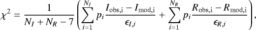 (3)
(3)
summing over all NI line transitions I and NR line ratios R to be included. The error depends on the observed tracer, we used the absolute error for the SPIRE observations (see Tables 5 and 6), a 30% error for the PACS data, 20% for (up)-GREAT/SOFIA and 10% for HIFI observations (see Sect. 2.6). We introduce a penalty factor, pi, to allow for weaker or stronger weighting of individual transitions or ratios in the numeric fit. χ2 is minimised in logarithmic space using the Nelder-Mead method assuming a shrink and contract ratio of 0.85, and a reflect a ratio of 3 using the software Mathematica4.
The best fitting model parameters, assuming pi = 1 for all i with the exception p(16−15) = 1000, are nn-c = 1.0 × 104 cm−3, Mn-c = 160 M⊙, χn-c = 830, ϕ = 0.94, and ⟨nc ⟩ = 1.8 × 106 cm−3, Mc = 1.1 M⊙, χc = 103 with a χ2 = 5.8. To assess the sensitivity of the result to the model parameters we varied all parameters by 20% (ϕ was varied by ±0.1) and present the resulting intensity variations as coloured bands around the best fit result. Across all intensities and ratios a 20% parameter variation changes the model intensities and intensity ratios by 46− 110%. The total model mass of 160 M⊙ is a good fit to the mass determined from the dust (166 M⊙), while the FUV field strengths are somewhat different from complementary estimates. These differences are discussed in Sect. 5.4.
Overall, the model intensity fit is very good with the exception of the [O I] 63 μm line, where the model intensities are about a factor of 10 too high, while the [O I] 145 μm line is well reproduced. The over-prediction of [O I] 63 μm intensity is a notorious problem that we attribute to an absorbing foreground layer (between the clumpy PDR and the observer), resulting in a significant optical depth along the line of sight. This is in agreement with recent SOFIA observations of star-forming regions were the [O I] 63 μm line was found to be heavily affected by foreground absorption while the upper [O I] 145 μm line is mostly unaffected (Schneider et al. 2018; Guevara et al. 2020). Figure 11 also shows that the [O I] 63 μm line arising from the PDR of the globule head suffers from significant self-absorption. A factor of ~10 in missing intensity is fully reasonable, although we cannot estimate the exact value, which is the reason for excluding the line from the numerical fit.
In order to asses the relative contribution of the clumpy and the non-clumpy component we separately plot the predicted emission in the left panel of Fig. 12. The three fine-structure lines show a different fraction of their emission coming from either component, resulting in a relatively sensitive probe to the degree of clumpiness in the region. We note that the [C II] emission receives a large contribution from the non-clumpy PDR. This points towards a scenario that the [C II] emission at velocities of the bulk emission of the globule is mostly caused by the external excitation from Cyg OB2. This is what we also concluded from the extended emission distribution seen in the [C II] maps. We note that ionised carbon is probably well mixed within the non-clumpy PDR component – and not only a thin external surface layer because we detect the rotation of the globule in [C II]. It is unlikely that it is only the external surface layer that is rotating. In addition, we presume that there is little [C II] emission coming from the ionised phase because the PDR model alone already well explains the observed intensities. However, we only modelled one point and cannot thus conclude over the full globule head.
Line fluxes and ratios for one position in the globule head.
Line fluxes and ratios for one position in the globule tail.
Summary of the best-fit models for the globule head and tail positions.
5.3 Non-clumpy model for the globule tail
The position we model in the globule tail (Fig. 4) is a more quiescent location than the one in the globule head since there are no internal sources and excitation happens only externally via the OB-cluster and by cosmic rays. We performed the fit with data smoothed to a larger beam size (40″) and tested again various models and found that a non-clumpy model with a single model component gives the best fitting results. These are displayed in Fig. 13 and show the SLEDs for the globule tail position with the observed CO line fluxes in 12CO and 13CO. The 12CO 10→9 and 9→8 and the 13CO 8→7 transitions have to be treated with care because the lines are weak and just above the noise level. The mass of the model was fixed to 70 M⊙, following the value determined from the dust column density (Sect. 3). All model parameters were varied and the colour-shaded areas in the left panel and coloured band in the right panel of Fig. 13 show how much the model intensities change. The illumination of the tail is assumed to be one-side only. The right panel displays the observational (blue) and model (red) fluxes for the [C II] and [C I] lines. Overall, a model with a UV field of around χ = 80 (corresponding to 137 G°) and a density of ~8 × 104 cm−3 with a filling factor of 0.3 fits our observations (χ2 = 1.9). The low model UV field is interesting, it is the lower limit from what was determined from the census of Cyg OB2 stars or the Herschel flux. Nevertheless, the non-clumpy fit for the globule tail is less convincing compared to the globule head model. The [C II] model intensities match the observed value and the 12CO lines are well reproduced up to 8→7. The two lowest 13CO lines fit the observations well, the upper lines are underestimated as well as the higher-J 12CO lines. Both [C I] fine-structure lines are significantly underestimated. The fit returned a filling factor of 0.3, namely, only 1/3 of the tail at the assumed position is supposedly illuminated by FUV. Comparing the[C II] contours in Fig. 4 with the beam size at the tail position would suggest a significantly larger filling of about 2/3. This emphasises the limits of the non-clumpy, single-component model that we applied. The next step could be a multi-component model, but this would require more data, for instance, the [O I] fine-structure lines. In addition, the high-J 13CO lines show a non-monotonous trend after the SLED peak, which is difficult to explain in a simple model.
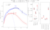 |
Fig. 12 PDR model results of the two-component globule model. Left panel: 12CO (blue lines) and 13CO (red lines) model SLED (spectral line energy distribution) together with the observed data (blue for 12CO and red for 13CO, respectively). We note that data points without error bars are excluded from the fit but are shown as a consistency check. The non-clumpy and clumpy contribution to the total SLED are displayed with dotted and dash-dotted lines, respectively. The hatched areas around the SLED’s indicate the model sensitivity to 20% variations of the model parameters. Centre panel: fine-structure line data. We note that the [O I] 63 μm line was excluded from the fit. The blue dots (with error bars) are the observations and the red dots are the model derived values with the red bands indicating the model response to 20% parameter variations, For each line intensity, we show forinformation their contribution from the non-clumpy and clumpy components with black and red crossed circles, respectively (with a slight offset to the right for easier reading). Right panel: behavior of the various line ratios with the same coding. |
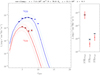 |
Fig. 13 PDR model results of the non-clumpy globule tail model. Left panel: 12CO (blue points and line) and 13CO (red points and line) model SLED (spectral line energy distribution). This is the best-fitting non-clumpy model. The colour-shaded areas give the range of models by varying all parameters by ± 20%. Right panel: observed (blue) and modelled (red) fine-structure line fluxes for this model, with the model variations indicated by the vertical red bands. Data points without error bars, namely, the two highest-J 12CO lines J = 10→9 and 9→8), are excluded from the fit, but shown to provide further information. |
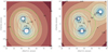 |
Fig. 14 FUV estimate for the globule. The three main stars A,B, and C are assumed to reside in the same plane on the sky. Spatial variations are shown in units of arcsec. The values of the contours are log χ where the Draine field χ has been computed from pure geometrical dilution. The two panels show χ excluding (left) and including (right) Star B. For information on the size scale, we plot three circles with radii of 10″ (red), 15″ (white), and 20″ (green) around a central position between Star A and C. |
5.4 UV field estimate for the globule head
We assume that the FUV field affecting the gas in the globule has two components. Firstly, an external radiation field, created by the massive stars of the Cyg OB2 association, and secondly, an internal radiation field created by the YSO embedded in the globule. In Schneider et al. (2012, 2016), we already presented an estimation of the FUV field based on the number of O-stars in Cyg OB2 and on the Herschel fluxes at 70 and 160 μm. We arrived to a value ofG° ≃ 313 (χ ≃ 183), considering 50 O-stars at the position of the globule at a distance of ~30 pc from Cyg OB2. These are upper limits since no extinction but only 1/r2 distance dilution was considered. We also did not take into account possible shadowing effects from the globule’s head. The number of O-stars in Cyg OB2, however, is uncertain and estimates range between ~50 (Comerón et al. 2002; Wright et al. 2015)and ~120 (Knödlseder 2000). The FUV field derived from the Herschel fluxes (right panel in Fig. 3) is ~150–200 G° for the globule tail, where we can assume that the illumination is only caused by the external radiation field. In summary, a value of 150–300 G° (88–176 χ) is probably a reasonable assumption for the total external radiation field impacting the globule. However, the field strength necessary toexplain the non-clumpy PDR emission is about two to three times stronger than that. Possible reasons for this discrepancy could come from a significantly higher number of OB stars in the cluster, as suggested by Knödlseder (2000). This would still be in conflict with the FUV estimates for the tail and it is unclear whether those can be explained by geometrical effects, for instance shielding or shadowing by the globule head. Alternative explanations for the higher FUV illuminating the external PDR could be an additional, possibly closer source such as the YSO B (see discussion below) or a much stronger fragmentation of the molecular gas in the head that allows the internally generated FUV to escape and also affect the external PDR.
Inside the globule head, the internal sources produce an internal Strömgren sphere embedded in the globule and illuminate the inner surface of the remaining spherical shell. Here, we estimate the strength for this internal radiation field for comparison and as a constraint for the PDR model. The FUV field of the YSOs is dominated by the internal sources, named Star A, B, and C in Djupvik et al. (2017) and we compute the FUV intensity by assuming stellar black-body emission with Teff = 22 600, 26 200, 26 200 K and stellar luminosities logL = 3,72, 4.04, 4.04, respectively, integrating over the FUV range from 910 to 3000 Å. The flux is diluted with 1/r2 and superposed in Fig. 14. Any additional attenuation, for instance, by dust is neglected, hence the result is an upper limit to the FUV field strength. Star B is slightly offset with regard to the H II region and the peaks of [C II] emission, so it is not clear whether this YSO is still embedded in the globule or whether it only appears related due to projection effects. However, the contribution of Star B to the radiation field close to our model position is relatively weak due to the larger distance. We thus assume that the internal FUV field is created by Stars A and C only. The PDR model fit gives a radiation field χc ~ 1000 for the clumpy component. A comparison with Fig. 14 shows that the FUV field estimated from the census of the stars and assuming no extinction is higher, typically a factor of 2–3. On the other hand, the FUV field from the Herschel fluxes is χ ~ 2500 in a 20″ beam at the peak position and χ ~ 1500 at the position where we perform the PDR modelling5. These values are in agreement with the PDR model estimates of the total FUV field (external and internal) which both contribute to the total continuum flux. The FUV derived from the Herschel fluxes and our model results differs from the census of the embedded stars. This cannot be explained via the dust attenuation of the FUV because any significant amount of dust in the H II region cavity that absorbs UV photons would still contribute to the IR continuum emission. The H II region cavity has a radius of ~15″–20″, which is consistent with the extent of the area of brightest IR and H2 and Brγ emission (Figs. 2 and 7 in Djupvik et al. 2017). A significantly larger cavity and, therefore, a lower FUV at the clumpy, internal PDR is unlikely. Most likely, our estimate of the FUV brightness of the embedded YSOs is too high due to lower Teff and log L.
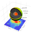 |
Fig. 15 Model geometry of the observed globule hosting two embedded YSO and an internal embedded cavity/H II region. The relative sizes of the individual shells are not shown to scale. The external non-clumpy PDR is shown as yellow outer shell, the internal, clumpy PDR is shown as golden clump ensembles between the embedded H II region and the molecular cloud shown as gray spherical shell. The image projected on the bottom plane is Spitzer 8 μm emission (for orientation, the flux values are not of interest here). The offsets are given in arcsec referring to the position RA(2000) = 20h33m49.95s, Dec(2000) = 40°07′42.75″. UV-radiation impacts externally via the Cyg OB2 cluster and internally via the YSOs. The cavity radius is approximately 15″–20″, determined from modelling and consistent with the region of brightest IR emission. |
5.5 Discussion of the model results
From the previous sections, we can see that the observed emission requires at least two PDR components: a non-clumpy, high mass component with a FUV illumination of χn-c ≈ 850, and a less massive clumpy PDR component that is about two orders of magnitude denser and requires a stronger FUV illumination of χc ≈ 1000. Given the geometrical constrains of the source, we propose the scenario outlined in Fig. 15. The embedded YSOs are creating a cavity/H II region embedded in the globule head. The inner surface of the remaining shell is compressed by the expanding H II region and possibly fragments into clumps, and is heated by the strong radiation of the YSOs.
The external surface of the globule is irradiated by the ambient FUV field and emits as a spherical (non-clumpy) PDR at a density of ~104 cm−3. The non-clumpy PDR component has a clump radius of ~60″, which is consistent with the observed extended FIR line emission of [C II] that traces mostly the outer PDR layer. Other lines with critical densities around 104 cm−3 and excitation temperatures around 50–100 K are the [C I] 2→1 and 1→0 lines and the mid-J CO lines. Their spatial emission distribution is also more extended than the emission lines of tracers that require higher densities and temperatures (such as the [O I] lines and the high-J CO lines, see Figs. A.1 and A.2). The latter have their origin in the PDR created at the internal surface of the cavity, which is clumpy and dense (~2 × 106 cm−3) and covers a relatively small volume due to its small mass. To test how realistic this scenario may be, we computed the thickness of the internal clumpy PDR layer because the clumpy PDR model fit returns the total PDR mass and volume (V = 7.2 × 1050 cm3) and this can be converted to a thickness as function of Rcavity. Accounting for irregularities and turbulent structures in the cavity surface, we can also apply a volume filling factor that describes how efficiently the clumpy PDR fill up the available volume.
Figure 16 shows how the PDR thickness varies as a function of Rcavity. We compare two volume filling scenarios. We find that the internal PDR layer is relatively thin with a thickness of ≈ 3−5 × 1014 cm (0.9–1.6 × 10⁻⁴ pc) only. We used the radius of the H II region cavity of ~15″, corresponding to 0.14 pc, to derive the thickness. Geometrically, this is consistent with our picture of the internal PDR surface. However, the spherical shell picture would decrease the volume and mass of the remaining globule and is inconsistent with the assumption of a full spherical (non-clumpy) PDR. Naturally, this mostly affects the molecular cloud tracers. In our model, however, the non-clumpy PDR contributes mostly to the [C II] emission and other surface tracers. We can, therefore, ignore this inconsistency at this point. We want to stress that the PDR model results were performed for all parameters independently. The proposed geometry also explains the over-predicted [O I] 63 μm intensity. In the model fit we simply add the clumpy and non-clumpy contribution. Geometrically, however, the non-clumpy PDR shell around the clumpy PDR is optically thick against the [O I] 63 μm line because the higher [O I] levels are not excited. We conclude that the resulting model components very nicely fit into the proposed geometry scenario and agree with complementary constraints such as the strength of the internal FUV field, the globule mass, and the observed [O I] self-absorption.
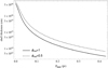 |
Fig. 16 Thickness of the internal PDR layer as function of cavity radius. Different lines correspond to variations in the volume filling factor of the ensemble. |
6 Conclusions and summary
We presented new spectroscopic FIR data for the globule IRAS 20319+3958 in Cygnus X South, located at 1.4 kpc distance, obtained with HIFI, PACS, and SPIRE on Herschel, and with upGREAT on SOFIA. The observations include all important FIR cooling lines in the interstellar medium, namely, the [C II] 158 μm line, the [O I] 63 μm and 145 μm lines, the [C I] 2→1, 1→0 lines, the mid- to high-J CO ladder (16→15 down to 3→2, and the [N II] lines at 205 μm and 122 μm. These tracers cover a large range of excitation temperatures and densities.
The [C II] line is the only FIR line that covers the full globule and is spectrally resolved. The kinematic [C II] distribution revealed several features. Firstly, the [C II] velocity map is consistent with rotation, that we attribute as a relic from the initial momentum the globule carried away while it was detaching from the molecular cloud. A comparison with simulations would help in exploring this possibility. Secondly, we detected a rather collimated high-velocity blue- and red-shifted [C II] outflow, associated with an embedded Herbig Be star. This star, together with two other systems of B-stars, is located inside the globule head and created an internal H II region. The outflow is not visible in the [O I] 63 μm line or in CO and we cannot discern the driving source, namely, the stellar wind of the Herbig Be star or the disk wind in case of an accretion disk.
We performed careful PDR modelling using the large observational data set of FIR lines (see above) for one position in the globule head and one in the tail. The objective was to determine the physical properties of the PDR components that are responsible for the emission of the various cooling lines and to establish a geometrical model for the globule head.
The best-fitting model is one with an extended (~60″ or ~0.4 pc), external non-clumpy PDR layer where most of the [C II] emission originates. The UV radiation of the ~30 pc distant Cyg OB2 cluster estimated from the stellar census of a few hundred G0 seems to be insufficient to account for the model FUV intensities of G0 ≈ 1500. A much larger stellar content of the OB cluster and/or additional possibly closer FUV sources may explain this discrepancy. The total mass from the PDR model is ~160 M⊙, which corresponds well to the mass determined from dust (166 M⊙), and an average density of 104 cm−3. Between the shell and the H II region cavity is a thin PDR layer (<0.1 pc) that is clumpy, dense (~2 × 106 cm−3), but not very massive (~1 M⊙) and illuminated by the embedded YSOs that create a radiation field of G0 > 103.
The tail position has no complex structure, the best fitting model is the one of a non-clumpy PDR with a mass of ~70 M⊙, illuminated by an external UV field of ~140 G° which corresponds to the lower UV field limit derived from the census of the stars and the Herschel flux estimate and may hint at additional shadowing of the tail by the globule head.
With this study, we establish evidence in support of our proposal from Schneider et al. (2012) and Djupvik et al. (2017) that the globule is an example of a region where intermediate-mass stars form in isolation within a single dense clump. We also show that PDR modelling of many cooling lines and a consideration of a complex geometry allows us to successfully explain the observed intensities.
Acknowledgements
This work was supported by the Agence National de Recherche (ANR/France) and the Deutsche Forschungsgemeinschaft (DFG/Germany) through the project “GENESIS” (ANR-16-CE92-0035-01/DFG1591/2-1). N.S. acknowledges support from the BMBF, Projekt Number 50OR1714 (MOBS - MOdellierung von Beobachtungsdaten SOFIA). This work isbased on observations made with the NASA/DLR Stratospheric Observatory for Infrared Astronomy (SOFIA). SOFIA is jointly operated by the Universities Space Research Association, Inc. (USRA), under NASA contract NAS2-97001, and the Deutsches SOFIA Institut (DSI) under DLR contract 50 OK 0901 to the University of Stuttgart. This work was supported by the German Deutsche Forschungsgemeinschaft, DFG project number SFB 956. G.J.W. gratefully acknowledges the receipt of an Emeritus Fellowship from The Leverhulme Trust. SPIRE has been developed by a consortium of institutes led by Cardiff University (UK) and including Univ. Lethbridge (Canada); NAOC (China); CEA, LAM (France); IFSI, Univ. Padua (Italy); IAC (Spain); Stockholm Observatory (Sweden); Imperial College London, RAL, UCL-MSSL, UKATC, Univ. Sussex (UK); and Caltech, JPL, NHSC, Univ. Colorado (USA). Thisdevelopment has been supported by national funding agencies: CSA (Canada); NAOC (China); CEA, CNES, CNRS (France); ASI (Italy); MCINN (Spain); SNSB (Sweden); STFC (UK); and NASA (USA). PACS has been developed by a consortium of institutes led by MPE (Germany) and including UVIE (Austria); KU Leuven, CSL, IMEC (Belgium); CEA, LAM (France); MPIA (Germany); INAF-IFSI/OAA/OAP/OAT, LENS, SISSA (Italy); IAC (Spain). This development has been supported by the funding agencies BMVIT (Austria), ESA-PRODEX (Belgium), CEA/CNES (France), DLR (Germany), ASI/INAF (Italy), and CICYT/MCYT (Spain).
Appendix A PACS and SPIRE spectroscopy
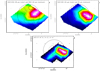 |
Fig. A.1 Various overlays of PDR lines observed with PACS. The colour range for the PACS [C II] data (top left) is 20 to 211 K km s−1, contours (1, 2, 3, 4 K km s−1) of [N II] emission are overlaid. The colour range for the PACS [O I] 145 μm data (top right) is 0 to 85 K km s−1, contours (10, 50, 90, 130, 170 K km s−1) of PACS [O I] 63 μm emission are overlaid. The colour range for the PACS CO 13→12 data (bottom) is 0 to 16 K km s−1, black contours (1, 4, 7, 11 K km s−1) of PACS CO 16→15 emission, and grey contours (5 to 25 by 5 K km s−1) of PACS CO 14→13 emission are overlaid. The ’finger’ of emission in CO 13→12 emission is probably an artefact since it is not visible in the CO 16→15 and 14→13 lines. The black triangle indicates the double system (Star A) of which at least one is a Herbig Be star, the white rectangle points to Star B with a B0.5 B1.5 spectral type, and the large black cross marks Star C, aresolved binary of which one is late O or early B star. The solid grey circle has a size of 20″ and the dashed one of 40″. This is the position for the flux determination for PDR modelling. |
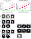 |
Fig. A.2 SPIRE spectroscopy results for the globule head. Top: FTS spectrum (blue) and line fit (red) for one spaxelof the SPIRE spectrometer for SLW (left) and SSW (right). The positions of the spectral lines included inthe fit are indicated. Bottom: Full SPIRE spectral maps showing the CO-ladder and the [C I] and [N II] lines.The intensity scale has been set relative to the peak brightness in each map with contour levels at 0.1, 0.3, 0.5, 0.7 and 0.9 of the peak (from blue to red). The SPIRE beam size varies between 31-43″ for SLW and 16-20″ for SSW (Swinyard et al. 2014). |
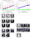 |
Fig. A.3 SPIRE spectroscopy results for the globule tail. Details are the same as Fig. A.2. |
Appendix B PDR model input parameters
Overview of the most important model parameters (see also Andree-Labsch et al. (2017)). All abundances are given with respect to the total H abundance.
References
- Alvarez-Gutierrez, R. H., Stutz, A. M., Law, C. Y., et al. 2021, ApJ, 908, 86 [CrossRef] [Google Scholar]
- Andree-Labsch, S., Ossenkopf-Okada, V., & Röllig, M., 2017, A&A, 598, A2 [NASA ADS] [CrossRef] [EDP Sciences] [Google Scholar]
- Asplund, M., Grevesse, N., & Sauval, A. J. 2005, ASP Conf. Ser., 336, 25 [Google Scholar]
- Bertoldi, F. 1989, ApJ, 346, 735 [NASA ADS] [CrossRef] [Google Scholar]
- Bisbas, T., Haworth, T., J., Barlow, M. J., et al. 2015, MNRAS, 454, 2828 [NASA ADS] [CrossRef] [Google Scholar]
- Black, J. H., & van Dishoeck, E. F. 1987, ApJ, 322, 412 [NASA ADS] [CrossRef] [Google Scholar]
- Cauley, P. W., & Johns-Krull, C. M. 2014, ApJ, 797, 112 [NASA ADS] [CrossRef] [Google Scholar]
- Cohen, M., Jones, B. F., & Walker, H. J. 1989, ApJ, 341, 908 [NASA ADS] [CrossRef] [Google Scholar]
- Comerón, F., & Torra, J. 1999, A&A, 349, 605 [Google Scholar]
- Comerón, F., Pasquali, A., Rodighiero, G., et al. 2002, A&A, 389, 874 [NASA ADS] [CrossRef] [EDP Sciences] [Google Scholar]
- Comerón, F., Djupvik, A., Schneider, N., & Pasquali, A. 2020, A&A, 644, A62 [Google Scholar]
- Cubick, M., Stutzki, J., Ossenkopf, V., et al. 2008, A&A, 488, 623 [NASA ADS] [CrossRef] [EDP Sciences] [Google Scholar]
- Dale, J. E., Haworth, T. J., & Bressert, E. 2015, MNRAS, 450, 1199 [NASA ADS] [CrossRef] [Google Scholar]
- de Graauw, T., Helmich, F. P., Philips, T. G., et al. 2010, A&A, 518, L4 [EDP Sciences] [Google Scholar]
- Diaz-Miller, R. I., Franco, J., & Shore, S. N. 1998, ApJ, 501, 192 [NASA ADS] [CrossRef] [Google Scholar]
- Djupvik, A. A., Comerón, F., & Schneider, N. 2017, A&A, 599, A37 [NASA ADS] [CrossRef] [EDP Sciences] [Google Scholar]
- Draine, B. T. 1978, ApJS, 36, 595 [NASA ADS] [CrossRef] [Google Scholar]
- Fuente, A., Martin-Pintado, J., Bachiller, R., et al. 2002, A&A, 387, 977 [NASA ADS] [CrossRef] [EDP Sciences] [Google Scholar]
- Gahm, G. F., Carlqvist, P., Johansson, L. E., & Nikolic, S. 2006, A&A, 545, 201 [Google Scholar]
- Goldsmith, P., Langer, W. D., Pineda, P., & Velusamy, T. 2012, ApJS, 203, 13 [Google Scholar]
- Griffin, M., Abergel, A., Abreau, A., et al. 2010, A&A, 518, L3 [EDP Sciences] [Google Scholar]
- Gritschneder, M., Naab, T., Walch, S., et al. 2009, ApJ, 694, L26 [NASA ADS] [CrossRef] [Google Scholar]
- Guevara, C., Stutzki, J., Ossenkopf-Okada, V., et al. 2010, A&A, 636, A16 [Google Scholar]
- Habing, H. J. 1968, Bull. Astron. Inst. Netherlands, 19, 421 [Google Scholar]
- Hester, J. J., Scowen, P. A., & Sankrit, R. 1996, AJ, 111, 2349 [NASA ADS] [CrossRef] [Google Scholar]
- Heyminck, S., Graf, U. U., Güsten, R., Stutzki, J., et al. 2012, A&A, 542, L1 [NASA ADS] [CrossRef] [EDP Sciences] [Google Scholar]
- Hollenbach, D., Kaufman, M. J., Neufeld, D., et al. 2012, ApJ, 754, 105 [NASA ADS] [CrossRef] [Google Scholar]
- Hsieh, C., Arcre, H. G., Maradones, D., et al. 2021, ApJ, 908, 92 [CrossRef] [Google Scholar]
- Johnstone, D., Hollenbach, D., & Bally, J. 1998, ApJ, 499, 758 [NASA ADS] [CrossRef] [Google Scholar]
- Kaufman, M. J., Wolfire, M. G., Hollenbach, D. J., & Luhman, M. L. 1999, ApJ, 527, 795 [Google Scholar]
- Knödlseder, J. 2000, A&A, 360, 539 [NASA ADS] [Google Scholar]
- Kronberger, M., Teutsch, P., Alessi, B., et al. 2006, A&A, 447, 921 [NASA ADS] [CrossRef] [EDP Sciences] [Google Scholar]
- Kumar, M., Keto, E., & Clerkin, E. 2006, A&A, 449, 1033 [NASA ADS] [CrossRef] [EDP Sciences] [Google Scholar]
- Langer, W. D., & Penzias, A. A. 1990, ApJ, 357, 477 [Google Scholar]
- Langer, W. D., Velusamy, T., Pineda, J., et al. 2010, A&A, 521, L17 [NASA ADS] [CrossRef] [EDP Sciences] [Google Scholar]
- Le Bourlot, J., Pineau Des Forets, G., Roueff, E., & Flower D. R. 1993, A&A, 267, A233 [Google Scholar]
- Lebouteiller, V., Cormier, D., Madden, S. C., et al. 2012, A&A, 548, A91 [NASA ADS] [CrossRef] [EDP Sciences] [Google Scholar]
- Lefloch, B., & Lazareff, B. 1994, A&A, 289, 559 [NASA ADS] [Google Scholar]
- Lefloch, B., Cernicharo, J., & Pardo, J. R. 2008, A&A, 489, 157 [NASA ADS] [CrossRef] [EDP Sciences] [Google Scholar]
- Levshakov, S. A., Reimers, D., & Henkel, C. 2016, A&A, 586, A126 [NASA ADS] [CrossRef] [EDP Sciences] [Google Scholar]
- Lim, B., Nazé, Y., & Gosset, E. 2020, MNRAS, 490, 440 [Google Scholar]
- Meijerink, R., & Spaans, M. 2005, A&A, 436, 397 [NASA ADS] [CrossRef] [EDP Sciences] [Google Scholar]
- Miao, J., White, G. J., Nelson, R. P., et al. 2006, MNRAS, 369, 143 [NASA ADS] [CrossRef] [Google Scholar]
- Miao, J., White, G. J., Thompson, M. A., et al. 2009, ApJ, 692, 382 [NASA ADS] [CrossRef] [Google Scholar]
- Motte, F., Zavagno A., Bontemps S., Schneider N., et al. 2010, A&A, 518, L77 [NASA ADS] [CrossRef] [EDP Sciences] [Google Scholar]
- Moura, T., Alencar, S. H. P., Sousa, A. P., et al. 2020, MNRAS, 494 [Google Scholar]
- Pilbratt, G. L., Riedinger, J. R., Passvogel, T., et al. 2010, A&A, 518, L1 [CrossRef] [EDP Sciences] [Google Scholar]
- Poglitsch, A., Waelkens, C., Geis, N., et al. 2010, A&A, 518, L2 [NASA ADS] [CrossRef] [EDP Sciences] [Google Scholar]
- Polehampton, E. T., Baluteau, J.-P., & Swinyard, B. M. 2005, A&A, 437, 957 [NASA ADS] [CrossRef] [EDP Sciences] [Google Scholar]
- Reipurth, B., & Schneider, N. 2008, Handbook of Star-forming Regions, (USA: ASP Monographs), 37 [Google Scholar]
- Risacher, C., Güsten, R., Stutzki, J., et al. 2016, A&A, 595, A34 [NASA ADS] [CrossRef] [EDP Sciences] [Google Scholar]
- Rodriguez, L. F., Zapata, L. A., & Dzib, S. A. 2014, ApJ, 793, L21 [NASA ADS] [CrossRef] [Google Scholar]
- Roelfsema, P. R., Helmich, F. P., Teyssier, D., et al. 2012, A&A, 537, A17 [NASA ADS] [CrossRef] [EDP Sciences] [Google Scholar]
- Röllig, M., Ossenkopf, V., Jeyakumar, S., et al. 2006, A&A, 451, 917 [NASA ADS] [CrossRef] [EDP Sciences] [Google Scholar]
- Röllig, M., Abel, N. P., Bell, T., et al. 2007, A&A, 467, 187 [NASA ADS] [CrossRef] [EDP Sciences] [Google Scholar]
- Röllig, M., Szczerba, R., Ossenkopf, V., & Glück, C. 2013, A&A, 549, A85 [NASA ADS] [CrossRef] [EDP Sciences] [Google Scholar]
- Rygl, K., Brunthaler, A., Sanna, A., et al. 2012, A&A, 539, A79 [NASA ADS] [CrossRef] [EDP Sciences] [Google Scholar]
- Schneider, N., Bontemps, S., Simon, R., et al. 2006, A&A, 458, 855 [NASA ADS] [CrossRef] [EDP Sciences] [Google Scholar]
- Schneider, N., Bontemps, S., Simon, R., et al. 2011, A&A, 529, A1 [NASA ADS] [CrossRef] [EDP Sciences] [Google Scholar]
- Schneider, N., Güsten, R., Tremblin, P., et al. 2012, A&A, 542, L18 [NASA ADS] [CrossRef] [EDP Sciences] [Google Scholar]
- Schneider, N., Bontemps, S., Motte, F., et al. 2016, A&A, 591, A40 [NASA ADS] [CrossRef] [EDP Sciences] [Google Scholar]
- Schneider, N., Röllig, M., Simon, R., et al. 2018, A&A, 617, A45 [NASA ADS] [CrossRef] [EDP Sciences] [Google Scholar]
- Schneps, M. H, Ho, P. T. P., & Barrett, A. H. 1980, ApJ, 240, 84 [NASA ADS] [CrossRef] [Google Scholar]
- Shirley, Y. L. 2015, PASP, 127, 299 [Google Scholar]
- Simon-Diaz, S., & Stasinska, G. 2011, A&A, 526, A48 [NASA ADS] [CrossRef] [EDP Sciences] [Google Scholar]
- Sofue, Y. 2020, MNRAS, 492, 5966 [NASA ADS] [CrossRef] [Google Scholar]
- Sternberg, A., & Dalgarno, A. 1995, ApJS, 99, 565 [NASA ADS] [CrossRef] [Google Scholar]
- Swinyard, B. M., Polehampton, E. T., Hopwood, R., et al. 2014, MNRAS, 440, 3658 [Google Scholar]
- Tielens, A. G. G. M., & Hollenbach, D. 1985, ApJ, 291, 722 [Google Scholar]
- Tremblin, P., Audit, E., Minier, V., & Schneider, N. 2012a, A&A, 538, A31 [NASA ADS] [CrossRef] [EDP Sciences] [Google Scholar]
- Tremblin, P., Audit, E., Minier, V., Schmidt, W., & Schneider, N. 2012b, A&A, 546, A33 [NASA ADS] [CrossRef] [EDP Sciences] [Google Scholar]
- Tremblin, P., Minier, V., Schneider, N., et al. 2013, A&A, 560, A19 [NASA ADS] [CrossRef] [EDP Sciences] [Google Scholar]
- Valtchanov, I., Hopwood, R., Bendo, G., et al. 2018, MNRAS, 475, 321 [NASA ADS] [CrossRef] [Google Scholar]
- Wakelam, V., & Herbst, E. 2008, ApJ, 680, 371 [NASA ADS] [CrossRef] [Google Scholar]
- Weingartner, J. C., & Draine, B. T. 2001, ApJ, 548, 296 [Google Scholar]
- White, G. J., Lefloch, B., Fridlund, C. V. M., et al. 1997, A&A, 323, 931 [NASA ADS] [Google Scholar]
- White, G. J., Nelson, R. P., Holland, W. S., et al. 1999, A&A, 342, 233 [NASA ADS] [Google Scholar]
- Wright, N., Drew, J. E., & Mohr-Smith, M. 2015, MNRAS, 449, 741 [NASA ADS] [CrossRef] [Google Scholar]
- Wolfire, M. G., McKee, C. F., Hollenbach, D., & Tielens, A. G. G. M. 2003, ApJ, 587, 278 [NASA ADS] [CrossRef] [Google Scholar]
- Wu, R., Polehampton, E. T., Etxaluze, M., et al. 2013, A&A, 556, A116 [NASA ADS] [CrossRef] [EDP Sciences] [Google Scholar]
The German REceiver for Astronomy at Terahertz frequencies. GREAT is a development by the MPI für Radioastronomie and the KOSMA/Universität zu Köln, in cooperation with the MPI für Sonnensystemforschung and the DLR Institut für Planetenforschung.
Note that the Habing field G° relates to the Draine field χ by χ = 1.71 G° where G° is the mean interstellar radiation field from Habing (1968); Draine (1978). We use both measures in this paper.
Mathematica 1 Version 12.1, Wolfram Research. Inc., Champaign, IL, 2020.
This estimation assumes that the dust in the PDR region and in the H II region cavity fully absorbs the emitted UV photons and re-emits in the FIR.
All Tables
Physical properties of the globule in total (Col. 2) and the head and tail (Cols. 3 and 4), respectively.
Overview of the most important model parameters (see also Andree-Labsch et al. (2017)). All abundances are given with respect to the total H abundance.
All Figures
|
Fig. 1 Three-colour (blue: 70 μm, green: 160 μm, red: 250 μm) image (Schneider et al. 2016) of the environment of Cyg OB2 with the globule IRAS 20319+3958, labeled as ‘globule’. The size of the image is ~1.5° × 1.4°, which corresponds to ~36 pc × 34 pc, assuming a distance of 1.4 kpc. The pillar indicated further east will be presented in another study. The most massive stars of the Cyg OB2 association are located in the northwest corner of the image (north is up, east to the left). |
| In the text | |
|
Fig. 2 Globule at IR- and FIR-wavelengths: Spitzer/IRAC 3.6–8 μm, Spitzer/MIPS at 24 μm, Herschel/PACS 70, and 160 μm and SPIRE 250, 350, and 500 μm (all units areMJy sr−1). The two lower right panels show velocity integrated molecular line emission of CS 2→1 and 12CO 3→2 in [K km s−1]. The beam is indicated in all panels with longer wavelength observations (starting with PACS 160 μm) in the lowerright corner. The Spitzer data were already displayed in Djupvik et al. (2017) and the Herschel data in Schneider et al. (2016). |
| In the text | |
|
Fig. 3 Herschel view of the globule. From left to right: column density (contours 1.3, 1.8, 2.3, 2.8 1022 cm−2), temperature (contours 17.1, 17.5, 19, 21, 23, 25 K), and UV-flux map (contours 150, 200, 500, 1000, 2000 G°) of the globule obtained from Herschel. These images are cut-outs from figures shown in Schneider et al. (2016). The column density and temperature maps have an angular resolution of 36″ and the UV map of 20″. These resolutions are indicated in the lower right corner of each panel. |
| In the text | |
|
Fig. 4 Line-integrated [C II] 158 μm emission of the globule obtained with HIFI on Herschel in the velocity range 0–15 km s−1. The blacktriangle indicates the double system (Star A) of which at least one is a Herbig Be star, the white rectangle points to Star B with a B0.5 - B1.5 spectral type, and the black cross marks Star C, a resolved binary of which one is a late O or early B star. The centre position (0,0) is at RA(2000) = 20h33m49.95, Dec(2000) = 40°07′42.75″. The [C II] beam is indicated in the lower left corner. The dashed lines indicate the vertical (north-south) cuts where we performed position-velocity maps and the dark grey circles mark the positions and the extend of the SPIRE beam for the longest wavelengths (FWHM ~ 40″) we used for PDR modelling. The position in the north is the globule ‘head’ and the one in the south the globule ‘tail’. |
| In the text | |
|
Fig. 5 Channel maps of [C II] emisson obtained with HIFI on Herschel from 2.5 to 13 km s−1. The symbols indicate the three stellar systems, similar to Fig. 4, except that here Star C is indicated with a white cross for better visibility. |
| In the text | |
|
Fig. 6 Position-velocity maps of the globule in [C II] for 5 vertical cuts cuts in declination at different RA offsets, indicated in Fig. 4. The zero-offset is at RA(2000) = 20h 33m50s and goes then in steps of 10″. The Dec (2000) range is 40°05′15″ to 40°09′45″. The bottom panel for cut = −40″ outlines with a white dashed rectangle the globule’s tail for which we show an overlay between two PV cuts in Fig. 7. |
| In the text | |
|
Fig. 7 Overlay between PV maps of the globule in [C II] for the −10″ (black contours) and −30″ (white contours) vertical cuts, indicated in Fig. 4. The dashed lines show the centre velocity of the globule’s tail for the cuts, i.e. 8.20 km s−1 for the −10″ cut and 7.35 km s−1 for the −30″ cut, respectively. |
| In the text | |
|
Fig. 8 Velocity map (first moment) of the [C II] emission, showing possible patterns of counter-clockwise rotation with the approximate axes indicated with dashed lines. The centre position (0,0) is at RA(2000) = 20h33m49.95, Dec(2000) = 40°07′42.75″. The [C II] beam is indicated in the lower left corner. We note that the axes for the globule head, where most of the mass resides, and the tail have not the same inclinations, and the velocity difference is larger for the head (~9.5 to ~6.9 km s−1) than for the tail (~8.3 to ~7.4 km s−1). The grey contour outlines the 2 K km s−1 contour level of [C II] emission, the symbols are the same as in Fig. 4. |
| In the text | |
|
Fig. 9 Continuum subtracted narrow-band image that contains the H2 1–0 S(1) ro-vibrational line at 2.122 μm (Djupvik et al. 2017) at ~2″ resolution with contours of velocity-integrated 12CO 3→2 emission (yellow, left panel) and velocity-integrated [C II] emission (red, right panel), both at 15″ resolution, overlaid. The CO contours go from 1 to 13 by 1.5 K km s−1 and the [C II] contours go from 5 to 155 by 15 K km s−1. The embedded stars A, B, and C are indicated. |
| In the text | |
|
Fig. 10 Map of H2 2.12 μm emission (Djupvik et al. 2017) with contours of [C II] outflow emission. The blue velocity range of the [C II] line ranges from 0 to 5 km s−1, contours go from 10 to 50 by 10 K km s−1. The red velocity range is 12–15 km s−1 and contoursgo from 3 to 13 by 2 K km s−1. The embedded stars and the [C II] beam size are indicated. |
| In the text | |
|
Fig. 11 Spectral maps of the [O I] 63 μm line (blue), the [C II] 158 μm line (red) and the CO 16→15 line (black) of the globule head in the velocity range −5 to 20 km s−1. The leftmostmain beam brightness temperature scale ranges from −0.2 to 2 K and is valid for [O I] and CO 16→15. The temperature scales at each panel are valid for [C II]. All data are smoothed to an angular resolution of 20″ and sampledon a grid of 20″ in order to increase the S/N. However, the CO 16→15 line was not observed at all positions (Sect. 2) so that we only plot the few spectra with observed emission above the 5σ level. The velocity resolution is 0.5, 0.7, and 0.6 km s−1 for [O I], [C II], and CO 16→15, respectively. The map centre position is RA(2000) = 20h33m50s, Dec(2000) = 40°08′36″. The approximate locations of the star systems are indicated. |
| In the text | |
|
Fig. 12 PDR model results of the two-component globule model. Left panel: 12CO (blue lines) and 13CO (red lines) model SLED (spectral line energy distribution) together with the observed data (blue for 12CO and red for 13CO, respectively). We note that data points without error bars are excluded from the fit but are shown as a consistency check. The non-clumpy and clumpy contribution to the total SLED are displayed with dotted and dash-dotted lines, respectively. The hatched areas around the SLED’s indicate the model sensitivity to 20% variations of the model parameters. Centre panel: fine-structure line data. We note that the [O I] 63 μm line was excluded from the fit. The blue dots (with error bars) are the observations and the red dots are the model derived values with the red bands indicating the model response to 20% parameter variations, For each line intensity, we show forinformation their contribution from the non-clumpy and clumpy components with black and red crossed circles, respectively (with a slight offset to the right for easier reading). Right panel: behavior of the various line ratios with the same coding. |
| In the text | |
|
Fig. 13 PDR model results of the non-clumpy globule tail model. Left panel: 12CO (blue points and line) and 13CO (red points and line) model SLED (spectral line energy distribution). This is the best-fitting non-clumpy model. The colour-shaded areas give the range of models by varying all parameters by ± 20%. Right panel: observed (blue) and modelled (red) fine-structure line fluxes for this model, with the model variations indicated by the vertical red bands. Data points without error bars, namely, the two highest-J 12CO lines J = 10→9 and 9→8), are excluded from the fit, but shown to provide further information. |
| In the text | |
|
Fig. 14 FUV estimate for the globule. The three main stars A,B, and C are assumed to reside in the same plane on the sky. Spatial variations are shown in units of arcsec. The values of the contours are log χ where the Draine field χ has been computed from pure geometrical dilution. The two panels show χ excluding (left) and including (right) Star B. For information on the size scale, we plot three circles with radii of 10″ (red), 15″ (white), and 20″ (green) around a central position between Star A and C. |
| In the text | |
|
Fig. 15 Model geometry of the observed globule hosting two embedded YSO and an internal embedded cavity/H II region. The relative sizes of the individual shells are not shown to scale. The external non-clumpy PDR is shown as yellow outer shell, the internal, clumpy PDR is shown as golden clump ensembles between the embedded H II region and the molecular cloud shown as gray spherical shell. The image projected on the bottom plane is Spitzer 8 μm emission (for orientation, the flux values are not of interest here). The offsets are given in arcsec referring to the position RA(2000) = 20h33m49.95s, Dec(2000) = 40°07′42.75″. UV-radiation impacts externally via the Cyg OB2 cluster and internally via the YSOs. The cavity radius is approximately 15″–20″, determined from modelling and consistent with the region of brightest IR emission. |
| In the text | |
|
Fig. 16 Thickness of the internal PDR layer as function of cavity radius. Different lines correspond to variations in the volume filling factor of the ensemble. |
| In the text | |
|
Fig. A.1 Various overlays of PDR lines observed with PACS. The colour range for the PACS [C II] data (top left) is 20 to 211 K km s−1, contours (1, 2, 3, 4 K km s−1) of [N II] emission are overlaid. The colour range for the PACS [O I] 145 μm data (top right) is 0 to 85 K km s−1, contours (10, 50, 90, 130, 170 K km s−1) of PACS [O I] 63 μm emission are overlaid. The colour range for the PACS CO 13→12 data (bottom) is 0 to 16 K km s−1, black contours (1, 4, 7, 11 K km s−1) of PACS CO 16→15 emission, and grey contours (5 to 25 by 5 K km s−1) of PACS CO 14→13 emission are overlaid. The ’finger’ of emission in CO 13→12 emission is probably an artefact since it is not visible in the CO 16→15 and 14→13 lines. The black triangle indicates the double system (Star A) of which at least one is a Herbig Be star, the white rectangle points to Star B with a B0.5 B1.5 spectral type, and the large black cross marks Star C, aresolved binary of which one is late O or early B star. The solid grey circle has a size of 20″ and the dashed one of 40″. This is the position for the flux determination for PDR modelling. |
| In the text | |
|
Fig. A.2 SPIRE spectroscopy results for the globule head. Top: FTS spectrum (blue) and line fit (red) for one spaxelof the SPIRE spectrometer for SLW (left) and SSW (right). The positions of the spectral lines included inthe fit are indicated. Bottom: Full SPIRE spectral maps showing the CO-ladder and the [C I] and [N II] lines.The intensity scale has been set relative to the peak brightness in each map with contour levels at 0.1, 0.3, 0.5, 0.7 and 0.9 of the peak (from blue to red). The SPIRE beam size varies between 31-43″ for SLW and 16-20″ for SSW (Swinyard et al. 2014). |
| In the text | |
|
Fig. A.3 SPIRE spectroscopy results for the globule tail. Details are the same as Fig. A.2. |
| In the text | |
Current usage metrics show cumulative count of Article Views (full-text article views including HTML views, PDF and ePub downloads, according to the available data) and Abstracts Views on Vision4Press platform.
Data correspond to usage on the plateform after 2015. The current usage metrics is available 48-96 hours after online publication and is updated daily on week days.
Initial download of the metrics may take a while.