© ESO 2021

1. Introduction

It has been known for decades that the rotation curve (RC) of a galaxy can be used as a proxy for the enclosed mass and its underlying distribution (Sofue & Rubin 2001; Salucci 2019). In the local Universe, we see the RCs of late-type galaxies¹ rising steeply in the inner regions and then flattening far beyond the disk edge² (Rubin et al. 1980; Persic et al. 1996; McGaugh 2016, and references therein). The steep rise in the inner regions is caused by the combination of a baryon-dominated disk plus a cored halo (Persic et al. 1996; Persic & Salucci 1988), while the flattening in the outer regions of the stellar disk and beyond implies dark matter (DM) dominance (Persic et al. 1996; Persic & Salucci 1988; Kassin et al. 2006; Martinsson et al. 2013; Courteau & Dutton 2015, and references therein). Recently, RC studies have been extended to higher redshifts (e.g., Di Teodoro et al. 2016; Genzel et al. 2017). However, as a result of observational challenges (e.g., a limited spatial resolution and moderate signal-to-noise ratio), the interpretation of the results remains ambiguous and still needs to converge to more concrete conclusions.

Recently, Genzel et al. (2017) and Lang et al. (2017) analyzed the RCs of star-forming galaxies (SFGs) at high-z and found a declining behavior with increasing radius; such behavior is only seen in very massive local SFGs, while the RCs of normal SFGs are remarkably flat and rarely decline (e.g., Rubin et al. 1980; Persic et al. 1996). Genzel et al. (2017) studied the individual RCs of six massive (log(M_* [M_⊙]) = 10.6−11.1) SFGs at redshift 0.9 ≤ z ≤ 2.4 in more detail. They showed declining RCs in two cases: first, when the individual RCs were normalized at R_max, where the amplitude of the rotational velocity is maximal; and second when the binned average of the six individual galaxies were normalized at the effective radius (R_e). Based on these results, Genzel et al. (2017) concluded that the fraction of DM within R_e is below 20%. Later, these results were confirmed by Lang et al. (2017), who obtained the stacked normalized RCs of 101 SFGs at 0.6 ≲ z ≲ 2.2 with stellar masses 9.3 ≲ log(M_* [M_⊙]) ≲ 11.5, where the normalization of RCs was performed at a “turnover radii”, where R_turn ∼ 1.65 R_e (for details see Lang et al. 2017). Both studies suggest that the declining behavior of RCs can be explained by a combination of high baryon fraction and extensive pressure support. Some other high-z studies of late-type and early-type galaxies also report similar low DM fractions within the effective radii (e.g., Burkert et al. 2016; Wuyts et al. 2016; Price et al. 2016; Übler et al. 2018).

On the other hand, Tiley et al. (2019b) studied the shape of RCs in ≈1500 SFGs at high-z (0.6 ≲ z ≲ 2.2) that have stellar masses 8.5 ≲ log(M_* [M_⊙]) ≲ 11.7. These authors used a similar stacking approach as Lang et al. (2017) and confirmed that the RCs are similar to those in Lang et al. (2017) (i.e., declining) if they are normalized at turnover radii. However, if instead the normalization was performed at 3 × R_D (≈1.77 R_e) they found flat or rising RCs. Moreover, Tiley et al. (2019b) reported a more than 50% DM fraction within 3.5 R_e, which is similar to local star-forming disk galaxies (Persic et al. 1996; Martinsson et al. 2013; Courteau & Dutton 2015). Finally, another study by Drew et al. (2018) analyzed a massive star-bursting galaxy at z = 1.55, which showed strong evidence of a flat RC between 6−14 kpc with a 44% DM fraction within the effective radius.

In order to resolve the serious issues raised by the previous literature on high-z RCs, we recently studied the intrinsic shape of RCs (Sharma et al. 2021) by means of 256 SFGs that have stellar masses 8.83 ≤ log(M_* [M_⊙] ≤ 11.32) at 0.7 ≲ z ≲ 1.04. In particular, we exploited KROSS data (Stott et al. 2016; Harrison et al. 2017) by employing different techniques than used in Genzel et al. (2017), Lang et al. (2017) and Tiley et al. (2019a). In brief, the key differences between our findings and previous studies lie in the modeling of the kinematics and the consideration of pressure support. We performed 3D forward modeling of data cubes using the ^3DBarolo code (Teodoro & Fraternali 2015), which improves the quality of resulting kinematics with respect to 2D kinematic modeling approaches. For pressure support, we employed the pressure gradient correction (PGC) method, which makes use of the full information available in the data cube and therefore gives better results than pressure support correction assuming isotropic and constant velocity dispersion; details are available in Sharma et al. (2021, appendix) and Kretschmer et al. (2021). Our results confirm that the outer (5 ≲ R ≲ 20 kpc) RCs of z ∼ 1 galaxies are flattish up to the last observation point and are very similar to the RCs of local star-forming disk galaxies. Noticeably, the inner (R ≲ 5 kpc) RCs of local SFGs are not flat; in this respect only future observations at high-z can show whether the similarity entirely remains or not.

In this paper we address the DM fraction in z ∼ 1 SFGs using the individual RCs derived in Sharma et al. (2021). The article is organized as follows: Sect. 2 contains a brief discussion of the data used; in Sect. 3 we compute and analyze the stellar, gaseous, and dynamical masses of the sample. In Sect. 4 we present the individual and averaged DM fractions. In Sect. 5 we discuss and compare our results with previous studies, and finally we critically summarize our findings in Sect. 6. Throughout the analysis we assumed a flat ΛCDM cosmology with Ω_m, 0 = 0.27, Ω_Λ, 0 = 0.73, and H₀ = 70 km s⁻¹.

2. Data

We utilize the KROSS dataset previously studied by Stott et al. (2016), Harrison et al. (2017), Tiley et al. (2019b,a) and Johnson et al. (2018)³. In particular, we studied a subsample of 344 KROSS SFGs in Sharma et al. (2021), where the kinematics of these objects were rederived from the original KROSS data cubes via the ^3DBarolo code (Teodoro & Fraternali 2015; Di Teodoro et al. 2016). This code accounts for the beam-smearing correction in 3D space and provides the moment maps, stellar surface brightness profile, RC, and dispersion curve (DC) along with the kinematic models. In addition, our RCs were corrected for pressure gradients that are likely to affect the kinematics of high-z galaxies. In the end, we analyzed only 256 rotation-dominated Quality 1 and 2 objects out of 344 KROSS objects, which we refer to as the Q12 sample; Sharma et al. (2021) gives details on the selection criteria and the dataset.

In this work, we use the Q12 sample to derive the DM fraction at various scale lengths (characteristic radii)⁴; those emerge from the local star-forming disk galaxies (given in Freeman 1970; Persic et al. 1996). According to which, the effective radius (half-light radius) R_e of a galaxy is defined to encompass the 50% of total integrated light. For an exponential surface brightness distribution I(r) ∝ exp(−r/R), R can be one of the various scale lengths, each of which is proportional to the stellar Freeman disk length R_D⁵ (Freeman 1970); for example, R_e = 1.69 R_D. Under the same assumption, the optical radius R_opt containing 83% of the integrated light becomes R_opt = 3.2 R_D. In the Q12 sample, the median effective radius is ∼3.1 kpc and the median optical radius is ∼5.9 kpc. This means that the effective radius of the majority of the sample falls below the resolution limit (∼4.0 kpc), since the median seeing is 0.5″ at z ∼ 0.9, while the optical radius is of the same order. Therefore, to be conservative and trace the DM fraction to the furthest point where we have data, we define the outer radius R_out = 5 R_D, which stays above the resolution limit in majority (≈99%) of the sample⁶.

Furthermore, for the accuracy and quality of the sample, we remove those galaxies that have R_out < 3.5 kpc (below the resolution limit), z < 0.65, and M_* < 10⁹ M_⊙⁷; in total we removed 31 galaxies. Our final sample contains 225 galaxies that have the inclination range 25° < θ_i ≤ 75°, the redshift range 0.76 ≤ z ≤ 1.04, the effective radii 0.08 ≤ log(R_e [kpc]) ≤ 0.89, and circular velocities 1.45 ≤ log(V_out [km s⁻¹]) ≤ 2.83, where V_out is calculated at R_out.

3. Analysis

In this section, we discuss the determination of stellar, gas, and dynamical masses.

3.1. Stellar masses

We adopt the stellar masses given by Harrison et al. (2017). These stellar masses were calculated using a fixed mass-to-light ratio following M_* = Υ_H × 10^{−0.4 × (M_H − 4.71)}, where Υ_H and M_H are the mass-to-light ratio and absolute magnitude in the H band (rest frame), respectively. Here Υ_H = 0.2, which is the median value of our sample obtained using the HYPERZ (Bolzonella et al. 2000) spectral energy distribution (SED) fitting tool; this tooluses a suite of spectral templates from Bruzual & Charlot (2003) and optical to near-infrared (NIR) photometry (U, B, V, R, I, J, H, and K)⁸.

The stellar masses calculated from a fixed mass-to-light ratio are slightly different from other studies of the same KROSS sample (e.g., Stott et al. 2016; Tiley et al. 2019b), in which different SED fitting procedures were used. However, the absolute median difference between the previous studies is about ±0.2 dex; see Fig. A.1. Therefore, we assigned a homogeneous uncertainty of ±0.2 dex on M_*, which is motivated by the aforementioned studies, as well as accounts for the typical uncertainty owing to low and high signal-to-noise photometry. Our sample covers the stellar mass range 9.0 ≤ log(M_* [M_⊙]) < 11.0. We note that we do not have very massive (log(M_*[M_⊙]) > 11.0) galaxies in our sample.

3.2. Molecular gas masses

To estimate the molecular gas mass (M_H2) of our galaxies, we adopt the relation given by Tacconi et al. (2018). These authors used a large sample of 1309 SFGs in the redshift range z = 0−4.4 with stellar masses log(M_*[M_⊙]) = 9.0−11.9 and star formation rates (SFRs) 10⁻² − 10² M_⊙ yr⁻¹. We stress that Tacconi et al. (2018) combined the three different methods to determine the molecular gas mass, each of which is related to one of the following: (1) CO line flux, (2) far-infrared dust SED, and (3) 1 mm dust photometry. Based on their composite findings, they established a single multidimensional unified scaling relation given by

$$\begin{array}{cc}\hfill log(M_{\mathrm{H}2})=[A+B\times & {(log(1+z)-F)}^2+C\times log(\delta \mathrm{MS})\hfill \\ \hfill & +D\times (log{M}_{\ast }-10.7)]+log(M_{\ast }),\hfill \end{array}$$(1)

where, A, B, C, D, and F are proportionality constants reported in Table 3b of Tacconi et al. (2018), MS is the main sequence (MS) relation of SFGs (see, Speagle et al. 2014), and δMS is the offset from MS line. In detail, δMS = sSFR/sSFR(MS;  z,  M_*), where sSFR is total specific SFR that is computed as $\mathrm{sSFR}=({\mathrm{SFR}}_{\mathrm{H}\alpha }^{\mathrm{int}})/M_{\ast }$, where ${\mathrm{SFR}}_{\mathrm{H}\alpha }^{\mathrm{int}}$ is the dust reddening-corrected H_α SFR. In this work the quantity ${\mathrm{SFR}}_{\mathrm{H}\alpha }^{\mathrm{int}}$ is derived by following the procedure of Stott et al. (2016); for details see Appendix B. The quantity sSFR(MS;  z,  M_*) is the specific SFR defined by Speagle et al. (2014) and can be computed as follows:

$$\begin{array}{cc}\hfill log(\mathrm{sSFR}(\mathrm{MS};z,M_{\ast }))& =(-0.16-0.026\times t_c)\hfill \\ \hfill & \times (log{M}_{\ast }+0.025)\hfill \\ \hfill & -(6.51-0.11\times t_c)+9,\hfill \end{array}$$

where t_c is the cosmic time, given by

$$\begin{array}{cc}\hfill log(t_c[\mathrm{Gyr}])& =1.143-1.026\times log(1+z)\hfill \\ \hfill & -0.599\times {log}^2(1+z)\hfill \\ \hfill & +0.528\times {log}^3(1+z).\hfill \end{array}$$

The full derivations of M_H2 and MS of galaxies at different redshifts are explained in greater detail in Tacconi et al. (2018) and Speagle et al. (2014), respectively.

The galaxies in our sample follow the relation between star formation rate and stellar mass given by Speagle et al. (2014), the so-called main sequence, with the following range of the relevant quantities: redshifts 0.77 ≤ z ≤ 1.04, stellar masses 9.0 ≤ log(M_* [M_⊙]) ≤ 10.97, and SFRs 0.49 ≤ log(SFR[M_⊙ yr⁻¹]) ≤ 1.77 (see Fig. B.1). Therefore, using the Eq. (1), we estimated the molecular gas mass of our galaxies.

3.3. Atomic gas masses

Observation of atomic hydrogen (HI) is challenging and can only be done in the radio wavelength by mapping the 21 cm fine-structure emission line produced by the spin-flip transition of the electron in the H atom. Currently, we cannot observe the 21 cm line at high-z, but with next-generation radio telescopes (e.g., ASKAP: Johnston et al. 2008; McConnell et al. 2016; Bonaldi et al. 2021) this should become possible in the near future. At present, the HI gas mass is typically inferred through the spectra of quasars (Péroux et al. 2003; Prochaska et al. 2005; Rao et al. 2006; Guimarães et al. 2009; Noterdaeme et al. 2012; Krogager et al. 2013; Moller et al. 2018, and reference therein), and scaling relations based on these observations and simulations. In our work, we use the scaling relation given by Lagos et al. (2011) for the atomic gas mass as follows:

$$\begin{array}{c}\hfill M_{\mathrm{HI}}=\frac{M_{\mathrm{H}2}}{0.01}(\frac{{10}^{10}{h}^{-1}{M}_{\odot }}{M_{\ast }}{)}^{0.8}{(1+z)}^{-3.3}.\end{array}$$(2)

The above relation agrees well with the global density of atomic and molecular hydrogen derived from damped Ly-α observations (Péroux et al. 2003; Rao et al. 2006; Noterdaeme et al. 2009) and predicts the H2 and HI mass function in the local Universe (Zwaan et al. 2005; Martin et al. 2010). Moreover, the Eq. (2) agrees very well with the scaling relation provided by a recent study of Calette et al. (2018) and DustPedia late-type galaxies (Casasola et al. 2020). Therefore, we use this relation to determine the HI masses of our sample. However, we emphasize that the M_HI computed using Eq. (2) gives the mass of the atomic gas, which corresponds to the scale of the molecular gas. In the outskirts of galaxies, M_HI is most likely different.

3.4. Baryonic mass estimates

In the Sects. 3.1–3.3, we derived the total stellar, molecular, and atomic mass content of our galaxies, which lead us to estimate the total baryonic mass as follows:

$$\begin{array}{c}\hfill M_{\mathrm{bar}}=M_{\ast }+M_{{\mathrm{H}}_2}+1.33M_{\mathrm{HI}},\end{array}$$(3)

where factor 1.33 accounts for the helium abundance. As a result, the total gas and stellar mass fraction can be written as f_star = M_*/M_bar, f_H2 = M_H2/M_bar, f_HI = M_HI/M_bar. In our sample of galaxies, we find the range 0.03 ≤ f_star ≤ 0.94 for the stellar mass fraction, 0.01 ≤ f_H2 ≤ 0.05 for the H2 (molecular gas) mass fraction, and 0.04 ≤ f_HI ≤ 0.95 for the HI (atomic gas) mass fraction. In Fig. 1 these fractions are plotted as a function of stellar mass and circular velocity (left and right panels, respectively) of a galaxy. Firstly, we notice that the molecular gas fraction is small in the visible region (∼5%) and remains constant as a function of the stellar mass and the circular velocity. Therefore, we argue that at z ∼ 1 molecular gas does not play a significant role in the kinematics, as occurs in the local SFGs.

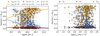Fig. 1. Stellar and gas mass fraction of our sample as a function of stellar mass and circular velocity (left and right panel, respectively) within the outer radius (Rout; i.e., visible region). The color code in both panels is the same and given as follows: the brown filled circles represent the molecular gas mass fraction (fH2 = MH2(<Rout)/Mbar(<Rout)), the orange filled circles indicate the star mass fraction (fstar = M*(<Rout)/Mbar(<Rout)), and the blue filled circles represent the atomic gas mass fraction (fHI = MHI(< Rout)/Mbar(< Rout)). A comparison study of local late-type galaxies from Calette et al. (2018) is drawn by solid lines; the color coding is same as the high-z objects.

Secondly, we observe a gradual decrease (increase) in the mass fraction of the atomic gas (stars) as a function of stellar mass. In particular, at the lower mass end (≤10^9.5 M_⊙) HI dominates, while at higher mass (≥10^10.2 M_⊙) stars dominate. At intermediate masses (10^9.5−10.0 M_⊙), the fraction of HI and stellar masses is almost 50–50% (see left panel Fig. 1).

We compare our baryon mass fraction results with local late-type galaxies (Calette et al. 2018) shown by solid lines in the left panel of the Fig. 1. We note that the objects with M_* > 10¹⁰ M_⊙ tend to have a similar gas and stellar mass fraction as local late-type galaxies, while low-mass M_* < 10¹⁰ M_⊙ objects seem to have a higher HI fraction independent of the local objects. We note that the H2 fraction remains the same. From the comparison of z ∼ 1 and z ∼ 0 baryon fractions, a key feature of galaxy evolution emerges, suggesting that the galaxies in our sample are in the middle of their evolutionary path⁹. The brightest (most massive) galaxies appear to be depleting their gas reservoir faster than the faintest galaxies, and because they exhibit this behavior, they appear to be present-day spiral galaxies.

Our goal is to calculate the DM fraction of our galaxies within R_e,  R_opt, and R_out, and therefore we must first determine the baryonic masses within these radii. In our previous work (Sharma et al. 2021), we found that the kinematics of the Q12 sample is similar to local star-forming disk galaxies. This suggests that the radial distribution of stellar and molecular gas masses within these galaxies can be well approximated by the Freeman disk (Freeman 1970):

$$\begin{array}{c}\hfill \begin{array}{cc}& M_{\ast }(<R)=M_{\ast }^{\mathrm{tot}}[1-(1+\frac{R}{R_{\ast }})exp\left(\frac{-R}{R_{\ast }}\right)]\hfill \\ \hfill & M_{H2}(<R)=M_{H2}^{\mathrm{tot}}[1-(1+\frac{R}{R_{H2}})exp\left(\frac{-R}{R_{H2}}\right)]\hfill \\ \hfill & M_{\mathrm{HI}}(<R)=M_{\mathrm{HI}}^{\mathit{tot}}[1-(1+\frac{R}{R_{\mathrm{HI}}})exp\left(\frac{-R}{R_{\mathrm{HI}}}\right)]\hfill \end{array}\end{array}$$(4)

where stars are assumed to be distributed in the stellar disk (R_* = R_D) known from photometry, discussed in Sect. 2. The molecular gas is generally distributed outward through the stellar disk (up to the length of the ionized gas R_gas); therefore, we take R_H2 ≡ R_gas. Here, we estimate the gas scale length R_gas by fitting the H_α surface brightness, which is discussed in Appendix C. Moreover, studies of local disk galaxies have shown that the surface brightness of the HI disk is much more extended than that of the H2 disk (Fu et al. 2010, see their Fig. 5); see also Leroy et al. (2008) and Cormier et al. (2016). Therefore, we assume R_HI = 2 × R_H2, which is a rough estimate, but still reasonable considering that at high-z no information is available on the M_HI (or M_H2) surface brightness distribution. Thus, the Eq. (4) allows us to estimate M_*, M_HI, and M_H2 within different radii (R_e,  R_opt, and R_out).

3.5. Dynamical mass estimates

The dynamical mass of a galaxy is defined as

$$\begin{array}{c}\hfill M_{\mathrm{dyn}}(<R)=\kappa (R)\frac{V^2(R)R}{G},\end{array}$$(5)

where V(R) is the circular velocity computed at radius R and κ(R) is the geometric factor accounting for the presence of a stellar disk alongside the spherical bulge and halo (see (Persic & Salucci 1990). For R_e, R_opt, and R_out, the values of κ are 1.2, 1.05, and 1.0, respectively. We favor a model-independent approach to determine the baryonic, dynamical, and DM masses at a given radius R, which differs from the standard RC mass decomposition method, where M_bar + M_DM ≃ M_dyn.

In Fig. 2 we show the results of the dynamical mass within R_out as a function of stellar and baryonic mass in the left and right panels, respectively. We find that the baryonic masses generally do not exceed the dynamical masses, and a DM component occurs in all objects, as implied independently of their RC profiles. Only a few galaxies are located in the forbidden region; however, they are consistent with M_bar ≤ M_dyn within the 1σ uncertainty intervals¹⁰.

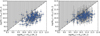Fig. 2. Stellar and baryonic masses as a function of dynamical mass (left and right panels, respectively), computed within Rout. The notations and color codes are the same in both panels and are given as follows: the blue filled circles represent the data, the dot-dashed black line shows the one-to-one plane, and the hatched-shaded gray area represents the forbidden region.

The bulge mass contribution within 5 kpc is negligible for local spirals; therefore, we do not model it. However, we emphasize that the stellar masses derived from the absolute H-band magnitude (via their M/L ratio) include the bulge mass. Moreover, the geometric parameter κ(R) in the dynamical mass calculation takes into account the distribution of the mass located in the bulge and in the disk.

4. Results

Given the information on bayonic and dynamical masses, the DM fractions within radius R can be computed as

$$\begin{array}{c}\hfill f_{\mathrm{DM}}(<R)=1-\frac{M_{\mathrm{bar}}(<R)}{M_{\mathrm{dyn}}(<R)}.\end{array}$$(6)

Therefore, using Eq. (6), we computed f_DM within R_e,  R_opt, and R_out for all galaxies. We note that owing to the limited spatial resolution in our RCs, the measurements of f_DM within R_e are less accurate than for R_opt and R_out. In the following subsection we demonstrate the DM fraction of individual objects as well as in terms of ensemble averages.

Individual galaxies. In the upper panel of Fig. 3, the DM fractions within R_out are plotted as a function of stellar mass; objects are color coded according to the circular velocity computed at R_out. First, it is noticeable that for a given stellar mass, the DM fraction seems to increase with increasing circular velocity, whereas the DM fraction shows a (shallow) decrease with increasing stellar mass. It is important to stress that both the baryonic and dynamical masses are determined with independent methods that have non-negligible errors; this affects the determination of the DM fraction and its errors (δf_DM(<R)). A typical value of δf_DM(<R_out) is ±0.2; however, at inner radii the uncertainties on the DM fraction reaches 0.4. Second, at R_out only ∼20% of the objects have f_DM(R_out) < 0.5. Noticeably, the objects with a low DM fraction (f_DM < 0.5) are not always the most massive but cover the broad stellar mass range log(M_* [M_⊙]) ≈ 9.2−10.7, irrespective of the local spirals (Salucci 2019). Moreover, only 8% objects fall in the forbidden region. This is very likely due to (i) the measurement errors discussed above, (ii) declining RCs, or (iii) determination of the RCs themselves. Some examples of such galaxies are shown in Fig. D.1.

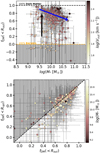Fig. 3. DM fraction of individual galaxies. Upper panel: dark matter fraction within Rout as a function of stellar mass (M*), color coded by the circular velocity (Vout) computed at Rout. The horizontal yellow and back dashed lines show the 100% baryon and DM regimes, respectively. The gray shaded area shows the forbidden region. The black arrow indicates that, for a given stellar mass, the fraction of DM in the galaxies increases with increasing circular velocity. The blue arrow shows a shallow decrease in the DM fraction with increasing stellar mass. Lower panel:fDM(<Ropt) vs. fDM(<Rout), color coded by stellar mass. The gray shaded area represents the not allowed region (i.e., fDM(<Rout) ≮ fDM(<Ropt)). The black dashed line shows the one-to-one relation. For the clarity of the figure (in the lower panel), objects below zero are not shown.

In the lower panel of Fig. 3, we investigate the increase in the DM fraction from the optical to the outer radius by plotting f_DM(R_opt) versus f_DM(R_out). As expected, 80% of the objects have f_DM(R_out) > f_DM(R_opt); that is, in the majority of the objects DM fraction increases with radius. However, we note that the perturbed or declining RCs severely affect the 20% of objects showing f_DM(R_out) < f_DM(R_opt). We will address this problem in our follow-up work, in which we plan to mass model the individual RCs using the component separation method and then determine the DM fraction at various radii. In this work, we proceed by averaging the various DM fractions.

Ensemble averages. In our work, we focused primarily on the study of individual objects. However, to compare our results with previous studies, we average the DM fraction in a suitable number of stellar mass bins. In particular, we employ affine binning of our 225 objects, keeping 50 objects per bin, and the last bin contains 25 objects. To perform the binning, we use the root mean square statistic (RMS), and the errors are estimated from bootstrap iterations. For each bin, we iterate 500 times, and 50% samples are taken in each run. Then the errors are assigned for the 68th, 95th, and 99th percentiles (of the scatter). The binning details are further explained and tabulated in Table 1. For simplicity, the averaged quantities are denoted by bar, for example, $\overline{M_{\ast }}$ and $\overline{f_{\mathrm{DM}}}$. We note that for the stacked data, we plot the 1σ error on DM fraction and its maximum scatter (1−3σ) is shown by the blue shaded regions. On the other hand, for stellar mass (being the running variable of the bin) we plot 3σ errors, which directly shows the maximum deviation from the mean ($\overline{M_{\ast }}$).

In upper panel of Fig. 4 we show the same results as in the upper panel of Fig. 3, but for the averaged dataset. From the upper panel, we can clearly see that the DM fraction weakly decreases with increasing stellar mass, and galaxies are DM dominated ($\overline{f_{\mathrm{DM}}}(<R_{\mathrm{out}})>50\%$) at any stellar mass value ($log(\overline{M_{\ast }}[M_{\odot }])\approx$ 9.5−10.0). Similarly, in the lower panel of Fig. 4 we show the same results as in lower panel of Fig. 3, but for the averaged dataset. In detail, we binned the lower panel of Fig. 3, in six f_DM(<R_out) bins namely [0.0–0.5, 0.5–0.6, 0.6–0.7, 0.7–0.8, 0.8–0.9, 0.9–1.0], using RMS statistics and errors are $\sqrt{{\sigma }_i^2/n}$ in each bin¹¹. We can clearly see that the $\overline{f_{\mathrm{DM}}}(R_{\mathrm{out}})$ is always larger than $\overline{f_{\mathrm{DM}}}(R_{\mathrm{opt}})$; that is, the mass of DM increases with radius. Both panels of Fig. 4 show that all of our ensemble averages have $\overline{f_{\mathrm{DM}}}\ge 50\%$ within R_opt till R_out, except for one data point at higher stellar mass. Nevertheless, ensemble averages of DM fraction in stellar mass bins, shown in Table 1, shows that $\overline{f_{\mathrm{DM}}}(<R_{\mathrm{out}})>\overline{f_{\mathrm{DM}}}(<R_{\mathrm{opt}})>\overline{f_{\mathrm{DM}}}(<R_e)$, which validates our measurements.

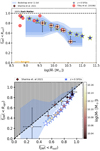Fig. 4. DM fraction of ensemble averages. Upper panel: dark matter fraction within Rout as a function of stellar mass (${\overline{M}}_{\ast }$). The brown hexagons with error bars shielded by big light-peach hexagons represent our averaged data, and the blue shaded area shows the 1, 2, and 3σ error at DM fraction. For comparison, we show the local star-forming disk galaxies (Persic et al. 1996) represented by the blue stars (in both panels), where the size of the marker represents the uncertainty in the values. The red hexagon represents the z ∼ 1 SFGs (Tiley et al. 2019b). Lower panel: $\overline{f_{\mathrm{DM}}}(<R_{\mathrm{opt}})$ vs. $\overline{f_{\mathrm{DM}}}(<R_{\mathrm{out}})$, color coded by stellar mass. The gray shaded area represents the theoretically not allowed region (i.e., $\overline{f_{\mathrm{DM}}}(<R_{\mathrm{out}})\nless \overline{f_{\mathrm{DM}}}(<R_{\mathrm{opt}}))$. The blue shaded area shows the maximum scatter in the relation. The lower panel interior of blue stars are color coded by stellar mass.

5. Discussion

In Sharma et al. (2021) we showed that the outer RCs of z ∼ 1 SFGs (having v/σ > 1) are similar to those of local (z ≈ 0) star-forming disk galaxies (Persic et al. 1996). In this work, we intend to compare the DM fraction of z ∼ 1 SFGs (v/σ > 1) with those of z ≈ 0 star-forming disks. The results are shown in Fig. 4. In the upper panel, we note that SFGs at z ∼ 1 and z ≈ 0 follow a similar trend in the $\overline{f_{\mathrm{DM}}}-{\overline{M}}_{\ast }$ plane; these SFGs also seem to have almost the same fraction of DM in the outer radius. In the lower panel of Fig. 4, we again observed a similar DM behavior as in the locals, but with a relatively higher DM fraction inside R_opt, which suggest that the radial profile of dark and luminous matter has evolved in the past 7 Gyr. This could be because at z ∼ 1 the DM halo has already formed, while the stellar disk inside R_opt is still in the process of formation.

Our results are in fair agreement with those of Tiley et al. (2019b) of similar SFGs. In particular, their sample lies in the redshift range 0.6 ≲ z ≲ 2.2; therefore, we narrowed down their sample to the galaxies that lie between 0.7 ≲ z ≲ 1.0 and over-plotted them in Fig. 4. As shown in the plot, there is a good agreement between the two studies. We note that Tiley et al. (2019b) computed $\overline{f_{\mathrm{DM}}}$ within 6 R_D, while we compute within R_out = 5 R_D.

Next, we compared our work with Genzel et al. (2017), Drew et al. (2018), and Übler et al. (2018); see right panel Fig. 5. In these studies, f_DM is computed within R_e, where our RCs are not spatially resolved and thus f_DM(<​​​R_e) is subject to larger uncertainties than f_DM within R_opt and R_out. Even so our four massive (log(M_*) ∼ 10.5−10.9) galaxies with f_DM(R_out) < 0.2 are very close to the results of Genzel et al. (2017) and Übler et al. (2018). Moreover, we agree closely with Drew et al. (2018). We also compare our work with the recent work of Genzel et al. (2020) (squares color coded for redshift). Their sample has seven objects with 9.0 ≲ log(M_*) ≲ 10.5 within the redshift range of 0.5 < z ≲ 1.0 and have a DM fraction ≥0.5; these values agree well with our individual DM fraction within R_e. However, the ensemble mean of DM fraction within R_e is always greater than 40%, showing dissimilarity with the majority of Genzel et al. (2020) objects. In particular, the mean of the massive bins for which ([$log({\overline{M}}_{\ast }),\overline{f_{\mathrm{DM}}},\overline{z}]=[10.6,0.53,0.9]$) shows a much higher DM fraction than Genzel et al. (2020). We would like to emphasize that the majority of their sample¹² have high stellar masses (log(M_*) > 10.5) and a low DM fraction (f_DM < 35%), which is not the case for our sample.

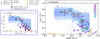Fig. 5. Comparison of averaged DM fraction (within Re) of our sample with previous high-z studies. Left panel: dark matter fraction as a function of baryon surface density ${\mathrm{\Sigma }}_{\text{Bar}}(<\text{}{R}_e)=M_{\text{bar}}(<\text{}{R}_e)/\pi R_e^2$. The brown hexagons with error bars shielded by big light-peach hexagons represent our averaged dataset, and individual galaxies are shown by small dots, color coded by redshift. The blue shaded area represents the 1−3σ error on the DM fraction. The dashed blue line shows the relation fDM(<​Re) = 1−10−0.34 + 0.51(log ΣBar − 8.5) given by Genzel et al. (2020) and their data are plotted in blue (z= 0.65−1.2) and red (z= 1.2−2.45) filled circles. Right panel: dark matter fraction as a function of stellar mass, color coded by redshift. Our dataset and its errors are presented in similar manner in both panels. Genzel et al. (2020) data are shown by filled squares. The measurements of Genzel et al. (2017), Drew et al. (2018), and Übler et al. (2018) are shown by yellow circles, a star and crosses, respectively, where the interior of each marker is color coded by redshift. The legend of the right plot is shown in the upper of left plot.

Moreover, we also compared our results with the f_DM(<R_e) versus Σ_Bar(<R_e) relation put forward by Genzel et al. (2020) (see left panel Fig. 5), where Σ_Bar(<R) = M_bar(<R)/πR². This relationship can be pivotal for both the DM nature and evolution of disk galaxies. We note that for low surface brightness (log(Σ_Bar(<R_e) M_⊙ kpc⁻²) < 8.7) galaxies, their relation is in fair agreement with our data, but at high Σ_Bar it underestimates DM fractions. We suspect that the high bulge-to-total (B/T) disk ratio used in Genzel et al. (2020) artificially reduces the DM within the effective radius.

Furthermore, while the DM -fractions at z ∼ 1 and z ∼ 0 are roughly the same, the scatter in the f_DM − M_* relation suggests that these galaxies are still in the process of building (or acclimating) the distribution of baryons and DM; that is, they are at different stages of their disk formation. However, it could also be due to the diversity in the DM halo properties (e.g., concentration and core radius or density), which are closely coupled to the properties of the baryonic matter (e.g., halo spin parameter and baryon fraction).

6. Summary

In this work, we have studied the fraction of DM in z ∼  1 SFGs. We used our previous study of RCs (Sharma et al. 2021) to compute accurate dynamical masses. In particular, we exploit 225 high-quality galaxies from the Q12 sample studied in Sharma et al. (2021). This sample lies between redshift 0.7 ≲ z ≲ 1.0 with stellar masses log(M_* [M_⊙]) = 9.0−11.0 and circular velocities log(V_out km s⁻¹) = 1.45−2.83. We estimate the total baryonic masses using scaling relations of atomic and molecular gas masses given by Lagos et al. (2011) and Tacconi et al. (2018) respectively (see Sects. 3.2–3.4). Subsequently, the DM fractions were computed using dynamical mass estimates from RCs. In Sect. 4, we showed that only ∼6% of objects have low DM fractions (0.0 < f_DM ≤ 0.2), but these objects are not necessarily massive. That is, a low DM fraction can also be found in low-mass galaxies (log(M_*[M_⊙]) < 9.5); however, uncertainties are higher there. Nonetheless, the majority (≳72%) of our sample contains DM-dominated (f_DM≳ 0.5−0.99) disks with a median radius ∼9 kpc (see Figs. 3–5). Our results are in agreement with a previous high-z study of the DM fraction of Tiley et al. (2019b) and are also consistent with local star-forming disk galaxies (Persic et al. 1996). We conclude that

• (1)

  The majority of star-forming disk-like galaxies (v/σ > 1) at 0.7 ≲ z ≲ 1.0 have outer (≈5−9 kpc) disks dominated by DM (see Figs. 3 and 4).

• (2)

  Baryon-dominated galaxies exist at high-z, similar to the local Universe, but they are very few (20%).

• (3)

  Star-forming galaxies at z ∼ 1 have similar or slightly higher (∼20%) DM fractions than the local ones within R_opt (see Fig. 4).

• (4)

  The scattering in the DM fractions at given stellar masses and circular velocities is larger at z ∼ 1 than at z ∼ 0. We interpret this as a consequence of ongoing galaxy formation or processes of evolution.

To gain a more fundamental understanding of the results presented in this work, as well as our earlier findings, we are working on the mass decomposition of RCs (Sharma et al., in prep.), which will shed light on the structural properties of DM and its interplay with baryons.

Acknowledgments

We thank the anonymous referee for their constructive comments and suggestions, which have significantly improved the quality of the manuscript. We thank A. Tiley for providing us the SED driven stellar masses of KROSS sample. We thank Andrea Lapi for his comments. G.S. thanks M. Petac for his fruitful discussion and various comments in the entire period of this work. GvdV acknowledges funding from the European Research Council (ERC) under the European Union’s Horizon 2020 research and innovation programme under grant agreement No 724857 (Consolidator GrantArcheoDyn).

References

Appendix A: SED-driven stellar masses

We discuss the stellar masses derived from two different approaches: SED fitting techniques (Tiley et al. 2019b) and fixed mass-to-light ratio stellar masses (Harrison et al. 2017). In particular, Harrison et al. (2017) uses H-band absolute magnitude to derive the fixed mass-to-light stellar masses; details are given in Sect. 3.1. On the other hand, Tiley et al. (2019b) stellar masses are derived using the LE PHARE (Arnouts et al. 1999; Ilbert et al. 2006) SED fitting tool. The LE PHARE compares the suites of modeled SED of objects from the observed SED. Where the observed SED of our sample is derived from optical and NIR photometric bands (U, B, V, R, I, J, H, and K), in some cases we also used the IRAC mid-infrared bands. In modeling, the stellar population synthesis model is derived from Bruzual & Charlot (2003), and stellar masses are calculated using Chabrier (2003) initial mass function (IMF). The LE PHARE routine fits the extinction, metallicity, age, star formation, and stellar masses and allows for a single burst, exponential decline, and constant star formation histories. Details of stellar-mass computation are available in Tiley et al. (2019b). In Fig. A.1, we show that the Tiley et al. (2019b) and Harrison et al. (2017) stellar masses are in full agreement with an intrinsic scatter of 0.2 dex. Tiley et al. (2019b) have not yet published the stellar masses of full KROSS sample, but we have access to them (in private communication); therefore, we are providing a consistency check.

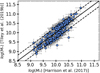Fig. A.1. Comparison of stellar masses derived from SED fitting (Tiley et al. 2019b) and fixed mass-to-light ratio (Harrison et al. 2017). The black solid and dashed line shows the one-to-one relation and 0.2 dex scatter, respectively.

Appendix B: Star formation rates

In general, SFRs in the ultra-violet, optical, or NIR (0.1–5 μm) probe the direct star light of galaxies, while SFRs in mid- or far-infrared (5–1000 μm) probe the stellar light reprocessed by dust. Therefore, the total SFR of any galaxy can be obtained by the linear combination of stellar and IR luminosities (Kennicutt 1998; Calzetti et al. 2007; Kennicutt & Evans 2012), for example,

$$\begin{array}{c}\hfill \mathrm{SFR}[M_{\odot }{\mathrm{yr}}^{-1}]=C_{H\alpha }{L}_{H\alpha }+C_{24\mathrm{\mu }\mathrm{m}}{L}_{24\mathrm{\mu }\mathrm{m}},\end{array}$$(B.1)

where C_Hα and C_24μm are the calibration constants, depends on star formation histories and IMFs. We can also derive the total SFR solely from stellar light (e.g., L_Hα), but then it requires an additional dust attenuation (or extinction) correction, which is defined as SFR^tot = SFR^obs × 10^A_ν, where A_ν is the attenuation correction at given wavelength.

In our sample we do not have possibility to trace the luminosities from UV to the mid- or far-infrared. However, we have access to H_α, H-, and K-band luminosities. Therefore, we estimated the SFR from H_α using Kennicutt (1998) relation given as

$$\begin{array}{c}\hfill {\mathrm{SFR}}_{H\alpha }[M_{\odot }{\mathrm{yr}}^{-1}]=4.677\times {10}^{-42}{L}_{H\alpha }[\mathrm{erg}{\mathrm{s}}^{-1}],\end{array}$$(B.2)

where calibration constants, C_Hα  =  4.677 × 10⁻⁴² M_⊙yr⁻¹erg⁻¹s, include the correction factor of 1.7 due to the (Chabrier 2003) IMF and Salpeter (1955) IMF used by Kennicutt (1998). Furthermore, we correct for dust reddening (extinction), based on the average value (A_Vgas = 1.43) derived in Stott et al. (2016) using the SED fitting. The A_Vgas = 1.43 is corrected for stars using A_Vgas/A_Vstar ≈ 1.7 (Calzetti et al. 2000; Pannella et al. 2015). In the Fig. B.1, we show the results and compare them with SFR-M_* relation given by Speagle et al. (2014), MS of SFGs. In particular, we derive the Speagle et al. (2014) MS relation between 0.7 ≤ z ≤ 1.2 including 0.3 dex error (shown by blue shaded area), and the best fit is given for z = 0.85, which has a slope 0.69. For our sample we derive the best fit using the least-squares method, which includes the errors in both axis. We obtain a slope of 0.79 ± 0.1 with intrinsic scatter 0.32 dex. Using a similar approach for the SFR determination, Stott et al. (2016) also observed a similar scatter in the SFR-M_* relation, which assures our measurements.

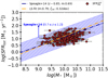Fig. B.1. Star formation rate (SFR) vs. total stellar mass (M*), tracing the MS of galaxies, where SFRtot = SFRHα corrected for dust reddening. The brown filled circles represent the data used in this work. The dashed-dotted orange line shows the least-squares fit to our data, and the blue line shows the Speagle et al. (2014) MS relation at z ∼ 0.85. The shaded blue region represents the MS limit between redshift 0.7 ≤ z ≤ 1.2, which includes 0.3 dex uncertainty at each redshift.

Appendix C: Gas disk length

We assume molecular and atomic gas has a spatial distribution described by an exponential profile

$$\begin{array}{c}\hfill {\mathrm{\Sigma }}_{\mathrm{gas}}={\mathrm{\Sigma }}_{0}exp(\frac{-R}{R_{\mathrm{gas}}}),\end{array}$$(C.1)

where Σ₀ is central surface density and R_gas is gaseous disk scale length. To estimate the value of R_gas, we fit the observed surface density of ionized gas¹³ following Eq. (C.1) using Markov Chain Monte Carlo (MCMC) sampling. During the fitting procedure Σ₀ and R_gas are the free parameter defined in the range 1 ≤ log(Σ₀) ≤ 9 and −0.5 ≤ log(R_gas [kpc]) ≤ 1.77, respectively. An example of best fit and posterior distribution is shown in Fig. C.1.

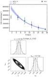Fig. C.1. Upper panel: observed surface brightness of Hα gas. The MCMC fit is shown in blue accompanied by 1σ error (blue shaded area). The first point (open square) is not used in fitting owing to the limitation assigned by Barolo (discussed in Sharma et al. 2021). The value Σ0 keeps the dimension units/kpc2, where units =ergs1cm−2μ−11 1e + 17 km s−1. Lower panel: posterior distribution of Σ0 and Rgas, where vertical dashed lines show the 16, 50, 84 percentiles from left to right, respectively.

Appendix D: Extra

Here, we provide examples of RCs which are providing wrong dynamical mass estimates either because of problem in the RC or in the determination of baryonic mass (see Fig. D.1).

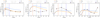Fig. D.1. Few example RCs for which either dynamical masses are unexpected or are a DM fraction. The color codes are as follows: Observed RC is shown by brown squares with the error bars connected with a black line; the orange and blue curves indicate the stellar and baryonic mass velocity curves derived assuming Freeman (1970) disk for given total M* and Mbar. The vertical red, light blue, and dashed blue lines represent the Re, Ropt, and Rout respectively. From left to right: first and second type of RCs seem to have either overestimated baryonic mass or wrong RC, which leads to smaller dynamical masses than baronic masses, and thus a negative DM fraction. The third type of RCs are announced declining, thus giving us fDM(<Ropt) > fDM(<Rout), which is generally not seen in the local SFGs. The fourth type of RCs are disturbed, thus discarded from the analysis.

With this paper, we release a catalogue of 225 SFGs studied in this work. In Table D.1, we describe the columns of the catalogue.

All Tables

All Figures

Fig. 1. Stellar and gas mass fraction of our sample as a function of stellar mass and circular velocity (left and right panel, respectively) within the outer radius (Rout; i.e., visible region). The color code in both panels is the same and given as follows: the brown filled circles represent the molecular gas mass fraction (fH2 = MH2(<Rout)/Mbar(<Rout)), the orange filled circles indicate the star mass fraction (fstar = M*(<Rout)/Mbar(<Rout)), and the blue filled circles represent the atomic gas mass fraction (fHI = MHI(< Rout)/Mbar(< Rout)). A comparison study of local late-type galaxies from Calette et al. (2018) is drawn by solid lines; the color coding is same as the high-z objects.

In the text

	Fig. 2. Stellar and baryonic masses as a function of dynamical mass (left and right panels, respectively), computed within Rout. The notations and color codes are the same in both panels and are given as follows: the blue filled circles represent the data, the dot-dashed black line shows the one-to-one plane, and the hatched-shaded gray area represents the forbidden region.
In the text

Fig. 3. DM fraction of individual galaxies. Upper panel: dark matter fraction within Rout as a function of stellar mass (M*), color coded by the circular velocity (Vout) computed at Rout. The horizontal yellow and back dashed lines show the 100% baryon and DM regimes, respectively. The gray shaded area shows the forbidden region. The black arrow indicates that, for a given stellar mass, the fraction of DM in the galaxies increases with increasing circular velocity. The blue arrow shows a shallow decrease in the DM fraction with increasing stellar mass. Lower panel:fDM(<Ropt) vs. fDM(<Rout), color coded by stellar mass. The gray shaded area represents the not allowed region (i.e., fDM(<Rout) ≮ fDM(<Ropt)). The black dashed line shows the one-to-one relation. For the clarity of the figure (in the lower panel), objects below zero are not shown.

In the text

Fig. 4. DM fraction of ensemble averages. Upper panel: dark matter fraction within Rout as a function of stellar mass (${\overline{M}}_{\ast }$). The brown hexagons with error bars shielded by big light-peach hexagons represent our averaged data, and the blue shaded area shows the 1, 2, and 3σ error at DM fraction. For comparison, we show the local star-forming disk galaxies (Persic et al. 1996) represented by the blue stars (in both panels), where the size of the marker represents the uncertainty in the values. The red hexagon represents the z ∼ 1 SFGs (Tiley et al. 2019b). Lower panel: $\overline{f_{\mathrm{DM}}}(<R_{\mathrm{opt}})$ vs. $\overline{f_{\mathrm{DM}}}(<R_{\mathrm{out}})$, color coded by stellar mass. The gray shaded area represents the theoretically not allowed region (i.e., $\overline{f_{\mathrm{DM}}}(<R_{\mathrm{out}})\nless \overline{f_{\mathrm{DM}}}(<R_{\mathrm{opt}}))$. The blue shaded area shows the maximum scatter in the relation. The lower panel interior of blue stars are color coded by stellar mass.

In the text

Fig. 5. Comparison of averaged DM fraction (within Re) of our sample with previous high-z studies. Left panel: dark matter fraction as a function of baryon surface density ${\mathrm{\Sigma }}_{\text{Bar}}(<\text{}{R}_e)=M_{\text{bar}}(<\text{}{R}_e)/\pi R_e^2$. The brown hexagons with error bars shielded by big light-peach hexagons represent our averaged dataset, and individual galaxies are shown by small dots, color coded by redshift. The blue shaded area represents the 1−3σ error on the DM fraction. The dashed blue line shows the relation fDM(<​Re) = 1−10−0.34 + 0.51(log ΣBar − 8.5) given by Genzel et al. (2020) and their data are plotted in blue (z= 0.65−1.2) and red (z= 1.2−2.45) filled circles. Right panel: dark matter fraction as a function of stellar mass, color coded by redshift. Our dataset and its errors are presented in similar manner in both panels. Genzel et al. (2020) data are shown by filled squares. The measurements of Genzel et al. (2017), Drew et al. (2018), and Übler et al. (2018) are shown by yellow circles, a star and crosses, respectively, where the interior of each marker is color coded by redshift. The legend of the right plot is shown in the upper of left plot.

In the text

	Fig. A.1. Comparison of stellar masses derived from SED fitting (Tiley et al. 2019b) and fixed mass-to-light ratio (Harrison et al. 2017). The black solid and dashed line shows the one-to-one relation and 0.2 dex scatter, respectively.
In the text

Fig. B.1. Star formation rate (SFR) vs. total stellar mass (M*), tracing the MS of galaxies, where SFRtot = SFRHα corrected for dust reddening. The brown filled circles represent the data used in this work. The dashed-dotted orange line shows the least-squares fit to our data, and the blue line shows the Speagle et al. (2014) MS relation at z ∼ 0.85. The shaded blue region represents the MS limit between redshift 0.7 ≤ z ≤ 1.2, which includes 0.3 dex uncertainty at each redshift.

In the text

Fig. C.1. Upper panel: observed surface brightness of Hα gas. The MCMC fit is shown in blue accompanied by 1σ error (blue shaded area). The first point (open square) is not used in fitting owing to the limitation assigned by Barolo (discussed in Sharma et al. 2021). The value Σ0 keeps the dimension units/kpc2, where units =ergs1cm−2μ−11 1e + 17 km s−1. Lower panel: posterior distribution of Σ0 and Rgas, where vertical dashed lines show the 16, 50, 84 percentiles from left to right, respectively.

In the text

Fig. D.1. Few example RCs for which either dynamical masses are unexpected or are a DM fraction. The color codes are as follows: Observed RC is shown by brown squares with the error bars connected with a black line; the orange and blue curves indicate the stellar and baryonic mass velocity curves derived assuming Freeman (1970) disk for given total M* and Mbar. The vertical red, light blue, and dashed blue lines represent the Re, Ropt, and Rout respectively. From left to right: first and second type of RCs seem to have either overestimated baryonic mass or wrong RC, which leads to smaller dynamical masses than baronic masses, and thus a negative DM fraction. The third type of RCs are announced declining, thus giving us fDM(<Ropt) > fDM(<Rout), which is generally not seen in the local SFGs. The fourth type of RCs are disturbed, thus discarded from the analysis.

In the text

References

- Arnouts, S., Cristiani, S., Moscardini, L., et al. 1999, MNRAS, 310, 540 [NASA ADS] [CrossRef] [Google Scholar]
- Bolzonella, M., Miralles, J. M., & Pelló, R. 2000, A&A, 363, 476 [NASA ADS] [Google Scholar]
- Bonaldi, A., An, T., Brüggen, M., et al. 2021, MNRAS, 500, 3821 [Google Scholar]
- Bruzual, G., & Charlot, S. 2003, MNRAS, 344, 1000 [NASA ADS] [CrossRef] [Google Scholar]
- Burkert, A., Schreiber, N. F., Genzel, R., et al. 2016, AJ, 826, 214 [NASA ADS] [CrossRef] [Google Scholar]
- Calette, A. R., Avila-Reese, V., Rodríguez-Puebla, A., Hernández-Toledo, H., & Papastergis, E. 2018, RMXAA, 54, 443 [NASA ADS] [Google Scholar]
- Calzetti, D., Armus, L., Bohlin, R. C., et al. 2000, ApJ, 533, 682 [NASA ADS] [CrossRef] [Google Scholar]
- Calzetti, D., Kennicutt, R. C., Engelbracht, C. W., et al. 2007, ApJ, 666, 870 [NASA ADS] [CrossRef] [Google Scholar]
- Casasola, V., Bianchi, S., De Vis, P., et al. 2020, A&A, 633, A100 [NASA ADS] [CrossRef] [EDP Sciences] [Google Scholar]
- Chabrier, G. 2003, PASP, 115, 763 [Google Scholar]
- Cormier, D., Bigiel, F., Wang, J., et al. 2016, MNRAS, 463, 1724 [CrossRef] [Google Scholar]
- Courteau, S., & Dutton, A. A. 2015, ApJ, 801, L20 [Google Scholar]
- Di Teodoro, E., Fraternali, F., & Miller, S. 2016, A&A, 594, A77 [NASA ADS] [CrossRef] [EDP Sciences] [Google Scholar]
- Drew, P. M., Casey, C. M., Burnham, A. D., et al. 2018, AJ, 869, 58 [NASA ADS] [CrossRef] [Google Scholar]
- Freeman, K. 1970, AJ, 160, 811 [NASA ADS] [CrossRef] [Google Scholar]
- Fu, J., Guo, Q., Kauffmann, G., & Krumholz, M. R. 2010, MNRAS, 409, 515 [NASA ADS] [CrossRef] [Google Scholar]
- Genzel, R., Schreiber, N. F., Ubler, H., et al. 2017, Nature, 543, 397 [NASA ADS] [CrossRef] [Google Scholar]
- Genzel, R., Price, S. H., Übler, H., et al. 2020, ApJ, 902, 98 [NASA ADS] [CrossRef] [Google Scholar]
- Guimarães, R., Petitjean, P., de Carvalho, R. R., et al. 2009, A&A, 508, 133 [NASA ADS] [CrossRef] [EDP Sciences] [Google Scholar]
- Harrison, C., Johnson, H., Swinbank, A., et al. 2017, MNRAS, 467, 1965 [NASA ADS] [CrossRef] [Google Scholar]
- Ilbert, O., Arnouts, S., McCracken, H. J., et al. 2006, A&A, 457, 841 [NASA ADS] [CrossRef] [EDP Sciences] [Google Scholar]
- Johnson, H. L., Harrison, C. M., Swinbank, A. M., et al. 2018, MNRAS, 474, 5076 [NASA ADS] [CrossRef] [Google Scholar]
- Johnston, S., Taylor, R., Bailes, M., et al. 2008, Exp. Astron., 22, 151 [NASA ADS] [CrossRef] [Google Scholar]
- Kassin, S. A., de Jong, R. S., & Weiner, B. J. 2006, ApJ, 643, 804 [NASA ADS] [CrossRef] [Google Scholar]
- Kennicutt, R. C. 1998, ARA&A, 36, 189 [Google Scholar]
- Kennicutt, R. C., & Evans, N. J. 2012, ARA&A, 50, 531 [NASA ADS] [CrossRef] [Google Scholar]
- Kretschmer, M., Dekel, A., Freundlich, J., et al. 2021, MNRAS, 503, 5238 [NASA ADS] [CrossRef] [Google Scholar]
- Krogager, J.-K., Fynbo, J. P. U., Ledoux, C., et al. 2013, MNRAS, 433, 3091 [NASA ADS] [CrossRef] [Google Scholar]
- Lagos, C. D. P., Baugh, C. M., Lacey, C. G., et al. 2011, MNRAS, 418, 1649 [NASA ADS] [CrossRef] [Google Scholar]
- Lang, P., Schreiber, N. M. F., Genzel, R., et al. 2017, AJ, 840, 92 [CrossRef] [Google Scholar]
- Leroy, A. K., Walter, F., Brinks, E., et al. 2008, AJ, 136, 2782 [Google Scholar]
- Martin, A. M., Papastergis, E., Giovanelli, R., et al. 2010, ApJ, 723, 1359 [NASA ADS] [CrossRef] [Google Scholar]
- Martinsson, T. P. K., Verheijen, M. A. W., Westfall, K. B., et al. 2013, A&A, 557, A131 [NASA ADS] [CrossRef] [EDP Sciences] [Google Scholar]
- McConnell, D., Allison, J. R., Bannister, K., et al. 2016, PASA, 33 [CrossRef] [Google Scholar]
- McGaugh, S. S. 2016, ApJ, 816, 42 [Google Scholar]
- Moller, P., Christensen, L., Zwaan, M. A., et al. 2018, MNRAS, 474, 4039 [NASA ADS] [CrossRef] [Google Scholar]
- Noterdaeme, P., Petitjean, P., Ledoux, C., & Srianand, R. 2009, A&A, 505, 1087 [NASA ADS] [CrossRef] [EDP Sciences] [Google Scholar]
- Noterdaeme, P., Laursen, P., Petitjean, P., et al. 2012, A&A, 540, A63 [NASA ADS] [CrossRef] [EDP Sciences] [Google Scholar]
- Pannella, M., Elbaz, D., Daddi, E., et al. 2015, ApJ, 807, 141 [NASA ADS] [CrossRef] [Google Scholar]
- Péroux, C., McMahon, R. G., Storrie-Lombardi, L. J., & Irwin, M. J. 2003, MNRAS, 346, 1103 [Google Scholar]
- Persic, M., & Salucci, P. 1988, MNRAS, 234, 131 [NASA ADS] [Google Scholar]
- Persic, M., & Salucci, P. 1990, MNRAS, 247, 349 [NASA ADS] [Google Scholar]
- Persic, M., Salucci, P., & Stel, F. 1996, MNRAS, 281, 27 [Google Scholar]
- Price, S. H., Kriek, M., Shapley, A. E., et al. 2016, ApJ, 819, 80 [NASA ADS] [CrossRef] [Google Scholar]
- Prochaska, J. X., Herbert-Fort, S., & Wolfe, A. M. 2005, ApJ, 635, 123 [NASA ADS] [CrossRef] [Google Scholar]
- Rao, S. M., Turnshek, D. A., & Nestor, D. B. 2006, ApJ, 636, 610 [NASA ADS] [CrossRef] [Google Scholar]
- Rubin, V. C., Ford, W. K., Jr, & Thonnard, N. 1980, AJ, 238, 471 [NASA ADS] [CrossRef] [Google Scholar]
- Salpeter, E. E. 1955, ApJ, 121, 161 [Google Scholar]
- Salucci, P. 2019, A&ARv, 27, 2 [CrossRef] [Google Scholar]
- Sharma, G., Salucci, P., Harrison, C. M., van de Ven, G., & Lapi, A. 2021, MNRAS, 503, 1753 [CrossRef] [Google Scholar]
- Sofue, Y., & Rubin, V. 2001, ARA&A, 39, 137 [NASA ADS] [CrossRef] [Google Scholar]
- Speagle, J. S., Steinhardt, C. L., Capak, P. L., & Silverman, J. D. 2014, AJ, 214, 15 [NASA ADS] [Google Scholar]
- Stott, J. P., Swinbank, A., Johnson, H. L., et al. 2016, MNRAS, 457, 1888 [NASA ADS] [CrossRef] [Google Scholar]
- Tacconi, L. J., Genzel, R., Saintonge, A., et al. 2018, ApJ, 853, 179 [NASA ADS] [CrossRef] [Google Scholar]
- Teodoro, E. D., & Fraternali, F. 2015, MNRAS, 451, 3021 [NASA ADS] [CrossRef] [Google Scholar]
- Tiley, A., Bureau, M., Cortese, L., et al. 2019a, MNRAS, 482, 2166 [NASA ADS] [CrossRef] [Google Scholar]
- Tiley, A. L., Swinbank, A., Harrison, C., et al. 2019b, MNRAS, 485, 934 [NASA ADS] [CrossRef] [Google Scholar]
- Wuyts, S., Förster Schreiber, N. M., Wisnioski, E., et al. 2016, ApJ, 831, 149 [NASA ADS] [CrossRef] [Google Scholar]
- Zwaan, M. A., Meyer, M. J., Staveley-Smith, L., & Webster, R. L. 2005, MNRAS, 359, L30 [NASA ADS] [CrossRef] [Google Scholar]
- Übler, H., Genzel, R., Tacconi, L. J., et al. 2018, AJ, 854, L24 [Google Scholar]