| Issue |
A&A
Volume 699, July 2025
|
|
|---|---|---|
| Article Number | A164 | |
| Number of page(s) | 28 | |
| Section | Extragalactic astronomy | |
| DOI | https://doi.org/10.1051/0004-6361/202347922 | |
| Published online | 04 July 2025 | |
Dark matter fraction in disk-like galaxies over the past 10 Gyr
1
Department of Physics and Astronomy, University of the Western Cape, Cape Town, 7535
South Africa
2
SISSA International School for Advanced Studies, Via Bonomea 265, I-34136
Trieste, Italy
3
INFN-Sezione di Trieste, Via Valerio 2, I-34127
Trieste, Italy
4
IFPU Institute for Fundamental Physics of the Universe, Via Beirut, 2, 34151
Trieste, Italy
5
University of Strasbourg, CNRS UMR 7550, Observatoire astronomique de Strasbourg, F-67000
Strasbourg, France
6
University of Strasbourg Institute for Advanced Study, 5 allée du Général Rouvillois, F-67083
Strasbourg, France
7
Department of Astrophysics, University of Vienna, Türkenschanzstraße 17, 1180
Vienna, Austria
8
Sterrenkundig Observatorium, Universiteit Gent, Krijgslaan 281 S9, 9000
Gent, Belgium
⋆ Corresponding author: gsharma@unistra.fr, gsharma@uwc.ac.za
Received:
8
September
2023
Accepted:
10
May
2025
We present an observational study of the dark matter fraction in star-forming disk-like galaxies up to redshift z ∼ 2.5 selected from publicly available integral field spectroscopic surveys: KMOS3D, KGES, and KROSS. To model the Hα kinematics of these galaxies, we employed 3D forward modeling, which incorporates beam-smearing and inclination corrections and yields rotation curves. Subsequently, we corrected these rotation curves for gas pressure gradients, resulting in circular velocity curves or ‘intrinsic’ rotation curves. Our final sample comprises 263 rotationally supported galaxies with redshifts ranging from 0.6 ≤ z < 2.5, stellar masses within the range 9.0 ≤ log(Mstar [M⊙]) < 11.5, and star formation rates between 0.49 ≤ log(SFR [M⊙ yr−1]) ≤ 2.5. We estimated the dark matter fraction of these galaxies by subtracting the baryonic mass from the total mass, where the total mass is derived from the intrinsic rotation curves. We provide novel observational evidence suggesting that at a fixed redshift, the dark matter fraction gradually increases with radius such that the outskirts of galaxies are dark matter dominated, similarly to local star-forming disk galaxies. This observed dark matter fraction exhibits a decreasing trend with increasing redshift, and on average, the fraction within the effective radius (up to the outskirts) remains above 50%, similar to the galaxies in the local Universe. We investigated the relationships between dark matter, baryon surface density, and the circular velocity of galaxies. We observed that low stellar mass galaxies, with log(Mstar [M⊙]) ≤ 10.0, undergo a higher degree of evolution, which may be attributed to the hierarchical merging of galaxies. We discuss several sources of uncertainties and current limitations in the field as well as their impact on the measurements of the dark matter fraction and its trend across galactic scales and cosmic time.
Key words: Galaxy: disk / Galaxy: evolution / Galaxy: kinematics and dynamics / galaxies: halos / galaxies: high-redshift
© The Authors 2025
 Open Access article, published by EDP Sciences, under the terms of the Creative Commons Attribution License (https://creativecommons.org/licenses/by/4.0), which permits unrestricted use, distribution, and reproduction in any medium, provided the original work is properly cited.
This article is published in open access under the Subscribe to Open model. Subscribe to A&A to support open access publication.
1. Introduction
Within the current standard model of structure formation, dark matter (DM), an enigmatic form of matter devoid of any electromagnetic interaction, is believed to represent most of the matter in the Universe (e.g., Peebles 1993). Despite its abundance, DM remains elusive and challenging to detect directly. Its existence is essentially inferred from the gravitational attraction it exerts on visible matter. In particular, flat outer galactic rotation curves have historically served as compelling evidence for the discrepancy between observed dynamics and the amount of baryons, leading to the hypothesis that galaxies are embedded within vast, extended halos of DM that largely surpass their luminous components in mass (e.g., Rubin et al. 1980; Bosma 1981; Salucci 2019, and references therein). Within the standard cold DM framework, cosmological simulations have corroborated that DM halos provide a gravitational scaffolding that allows galaxies to form and maintain their structures (Angulo & Hahn 2022, and references therein), although so-called small-scale challenges remain (e.g., Bullock & Boylan-Kolchin 2017, Sales et al. 2022).
The amount of DM within galaxies varies depending on their baryonic mass, size, and environment, underscoring its critical influence on their overall dynamics and evolution. Observations of nearby star-forming galaxies indeed yield a DM fraction between 40% and 50% in their inner region within the projected half-light radius (Re) and between 70% and 90% within 3Re, which encompasses most of the galaxy’s light (Kassin et al. 2006; Martinsson et al. 2013; Courteau & Dutton 2015). Observations of early-type galaxies often reveal lower DM fractions in the inner regions (≲20% within Re, Cappellari et al. 2013), which tend to rise with increasing stellar mass in galaxies with masses Mstar ≥ 1010 M⊙, but similarly high fractions in the outskirts (70 − 90% within 5Re, Harris et al. 2020). One reason for this may be that early-type galaxies may have experienced extensive baryonic processes over their lifetimes. These processes can affect both the distribution of baryons and that of DM, as simulations have shown that baryonic processes can expel DM over a time span of several gigayears (Pontzen & Governato 2012). In particular, feedback processes such as supernova explosions, stellar winds, and active galactic nuclei stir the interstellar medium of galaxies and launch powerful gas outflows, which induce fluctuations in the gravitational potential that can in turn affect DM and diminish its fraction in the inner region of all type of galaxies (e.g., Pontzen & Governato 2014; Dutton et al. 2016; El-Zant et al. 2016; Freundlich et al. 2020; Dekel et al. 2021; Li et al. 2023). These processes can indeed dynamically heat up the DM and lead to the formation of constant DM density cores rather than steep cusps. Therefore, characterizing the DM fraction and its evolution with cosmic time not only enables better understanding of the influence of the DM distribution on galaxy formation and evolution, but it also provides valuable insights into the physical processes that govern galaxies and contributes to testing of the implementation of feedback processes in simulations.
In the past decade, integral field units (IFUs) in galaxy surveys have opened up new possibilities for studying the spatially resolved kinematics of high-z galaxies. For example, a review by Förster Schreiber & Wuyts (2020) notably shows that by using the resolved kinematics, it is now possible to obtain the rotation curves (RCs) of galaxies up to z ∼ 2.5. These RCs allow one to probe the baryon and dark matter content on galactic scales as well as their distribution and physical properties. Genzel et al. (2017) and Lang et al. (2017) were the first to analyze the RCs of star-forming galaxies (SFGs) at high-z (0.6 ≤ z ≤ 2.6), and they found them to be declining; such behavior is only seen in local massive (very high surface brightness) SFGs, while the RCs of most normal SFGs are remarkably flat and rarely decline (e.g., Rubin et al. 1980 and Persic et al. 1996). Both studies (Genzel et al. 2017 and Lang et al. 2017) suggest that the declining behavior of rotation curves can be explained by a combination of high baryon fraction and pressure support in the inner regions. Some other high-z studies of late-type and early-type galaxies also report similar low dark matter fractions within the effective radii (e.g., Burkert et al. 2016; Wuyts et al. 2016; Price et al. 2016; Übler et al. 2018). Conversely, Tiley et al. (2019a) studied the shape of rotation curves in ≈1500 SFGs at 0.6 ≲ z ≲ 2.2 and reported flat rotation curves similar to local SFGs. Moreover, Tiley et al. (2019a) reported a more than 50% dark matter fraction within 3.5 Re, which is similar to local star-forming disk galaxies (Persic et al. 1996; Martinsson et al. 2013; Courteau & Dutton 2015).
In another follow-up study, Sharma et al. (2021a) studiedK-band Multi-Object Spectrograph (KMOS; Sharples 2014) Redshift One Spectroscopic Survey (KROSS) data (Stott et al. 2016) and derived the observed rotation and dispersion curves using 3D forward modeling. These observed rotation curves were then converted into intrinsic RCs by correcting issues related to high-z measurements, such as beam smearing and pressure gradient. This provided them with a large sample of more than 200 flat rotation curves of disk-like galaxies at z ∼ 1 (i.e., 6.5 Gyr look-back time). In Sharma et al. (2021b), the authors employed these intrinsic rotation curves to estimate the invisible mass fraction needed to recover observed kinematics without invoking any DM halo model (such as the cuspy NFW from Navarro et al. 1996 or the cored Burkert 1995). In this technique, stellar masses (Mstar) are estimated by fitting the spectral energy distribution (SED) of the galaxies and the gas (molecular and atomic) masses by means of the scaling relations by Tacconi et al. (2018) and Lagos et al. (2011). Assuming an exponential thin disk distribution, they estimated the contribution of baryons to total mass at different scale radii (disk radius: 0.59Re, optical radius: 1.89Re, and outer radius: 2.95Re), where the total mass is the dynamical mass (Mdyn ∝ G−1V2R) computed directly from the intrinsic rotation curves.1 This work showed that the majority (> 72%) of star-forming galaxies in the KROSS sample at z ∼ 1 haveDM-dominated (> 60%) outer disks (∼5 − 10 kpc), which agrees well with local SFGs.
Recently, various other studies have investigated the DM fraction within Re, including works by Genzel et al. (2020), Price et al. (2021), Bouché et al. (2022), Nestor Shachar et al. (2023), and Puglisi et al. (2023). In this article, our focus is on studying the DM fraction within different galactic scales, ranging from Re up to approximately 3Re (≈Rout).
In particular, we expand our understanding of the DM fraction by incorporating a larger sample and extending the redshift range beyond that of Sharma et al. (2021b). We present a comprehensive investigation using data from the KMOS3D survey (Wisnioski et al. 2019) and the KMOS Galaxy Evolution Survey (KGES; Tiley et al. 2021) and previously analyzed KROSS data, covering a redshift range of 0.6 < z < 2.5.
Our primary objectives are to test the rotation curve analysis method established in Sharma et al. (2021a,b), examine the redshift evolution of DM fractions across galactic scales, and explore questions related to the assembly history of galaxies. Most importantly, we demonstrate how current constraints on accurately accounting for baryonic content result in substantial uncertainties, both statistical and systematic, in estimating the DM mass of galaxies. By reducing these uncertainties, we as a community have the potential to make a significant leap forward in our understanding of galaxy evolution. The structure of this article is as follows: In Section 2, we provide an overview of the datasets utilized in this study. Section 3 describes the employed kinematic modeling techniques, the analysis of its outputs, and the establishment of a robust final sample used throughout this work. Moving to Section 4, we investigate the data for potential discrepancies, present the results of the DM fraction at different galactic scales and cosmic time, and discuss the correlations between dark matter fraction, baryonic surface density, and circular velocity. Section 5 discusses potential caveats associated with this study. Subsequently, in Section 6, we delve into a detailed discussion of the main results. Finally, we summarize our findings in Section 7. Throughout the analysis we assumed a flat ΛCDM cosmology with Ωm, 0 = 0.27, ΩΛ, 0 = 0.73, and H0 = 70 km s−1.
2. Datasets
In this study, we utilize publicly available high-z galaxy surveys conducted with the KMOS instrument (Sharples 2014), namely the KMOS3D survey (Wisnioski et al. 2019), KGES (Tiley et al. 2021)2, and KROSS (Stott et al. 2016). KMOS is a second-generation spectrograph located at the Very Large Telescope (VLT), which indeed offers unique advantages for constraining the dark matter fraction in high-z galaxies. One key feature of KMOS is its capability for integral field spectroscopy, which enables efficient and rapid surveying of a large number of galaxies. Moreover, KMOS operating capability in wavelength range 0.778 − 2.481 μm facilitates the detection of rest-frame optical emission from high-z, such as Hα (λrest = 0.6562 μm). Additional benefit of this broad wavelength coverage is its ability to provide crucial information regarding the stellar populations, star-formation rates, kinematics and dynamics of distant galaxies. In this work, we specifically investigate the dynamics of distant galaxies and analyze the results in the light of prevalent issues, such as, observational uncertainties (e.g., noise), kinematic modeling, and dynamical models.
2.1. KMOS3D
All objects of the KMOS3D survey are drawn from the 3D-HST survey (Brammer et al. 2012; Skelton et al. 2014; Momcheva et al. 2016) within three extra-galactic fields (COSMOS, Scoville et al. 2007; GOODS-S, van Dokkum & Brammer 2010; and UDS, Lawrence et al. 2007) covering a wide redshift range (0.7 < z < 2.7). The KMOS3D observations in the YJ−, H−, and K−bands cover the Hα emission line at redshift 0.7 < z < 1.1, 1.2 < z < 1.8, and 1.9 < z < 2.7, respectively. In all three filters average seeing conditions –expressed as the full width half maximum (FWHM) of the point spread function (PSF) – are less than or equal to 0.55″. We begin with analyzing all Hα cubes, and adopt the catalogs released in Wisnioski et al. (2019). From the physical property catalog (Wisnioski et al. 2019, Table 5), we mainly work with quantities such as galaxy-IDs, sky-coordinates, redshift, magnitude, seeing (FWHM), HST-axis ratios, effective radius, stellar masses, and star-formation rates. The aperture size of the Hα datacubes is 1.5″ in radius. The other details, such as IDs, detection and non-detection flags, of Hα datacubes are given in the catalog associated with Table 6 of Wisnioski et al. (2019).
Physical properties of galaxies: Stellar masses in the KMOS3D survey (Wisnioski et al. 2019) were derived from SED modeling using the FAST fitting code (Kriek et al. 2009), assuming exponentially declining star-formation histories (τ > 300 Myr), solar metallicity, a Chabrier (2003) initial mass function (IMF), and stellar population synthesis models derived from Bruzual & Charlot (2003). The dust attenuation was modeled using the Calzetti et al. (2000) reddening law, with visual extinctions in the range 0 < Av < 4. The full KMOS3D sample covers the stellar mass range 8.3 ≤ log(Mstar [M⊙])≤11.7. The effective radius of galaxies are computed from high-resolution CANDELS H-band photometry (Skelton et al. 2014), covering −0.6 ≤ log(Re [kpc])≤1.5. The star-formation rate is derived using a cross-calibrated ladder of SFR indicators (Wuyts et al. 2011). The statistical uncertainty in stellar masses and star-formation rates is assumed to be 10%. Additionally, following Pacifici et al. (2023), we incorporate a systematic uncertainty of 0.14 dex in the stellar mass and 0.25 dex in the star formation rate (SFR). To obtain the inclination angle, we use the axis-ratio a/b from Wisnioski et al. (2019) and convert it into inclination θi according to
where q0 is the intrinsic axial ratio of an edge-on galaxy (e.g., Tully & Fisher 1977), which could in principle have values in the range 0.1–0.65 (e.g., Weijmans et al. 2014); here, we use the commonly assumed value q0 = 0.2, which is applicable for thick discs commonly found at high-z (Harrison et al. 2017). The resulting inclinations cover a broad range between ≈10° −85°. The kinematic/photometric position angles (PA) are not in the public release of KMOS3D data and obtained through kinematic modeling of the datacubes as discussed in Appendix B. The central positions of the sources are similarly re-derived during the kinematic modeling.
Primary selection criteria: The Wisnioski et al. (2019) catalog contains 627 galaxies with spectroscopically confirmed redshift (see their Table 6), which we refer to as the parent sample. From those, we selected Hα-detected galaxies (i.e., with FLAG 0,1 in the catalog) with high inclination angle (25° ≤θi ≤ 75°)3.
This left us with 448 objects. Before performing the kinematic modeling, we inspected their signal-to-noise ratio (S/N) and Hα images as discussed in Appendix A and demonstrated in Figures A.1 and A.2. The signal-to-noise ratio is defined as signal/noise, and it is computed from integrated spectra of flux and noise cubes. The S/N > 3 threshold is the requirement of kinematic modeling tool 3DBarolo (Teodoro & Fraternali 2015; Di Teodoro et al. 2016) to produce accurate kinematics. Based on this quantitative and qualitative assessment of dataset, we divide the 448 objects of the sample in three categories: Q1: S/N > 3 and sharp Hα image; Q2: S/N ≥ 3 and moderately visible source; Q3: either S/N < 3 or no appearance of the source in the Hα image. We discard all the Q3 galaxies, which yields a final sample of 265 sources for kinematic modeling. The distributions of inclination angle, stellar mass, effective radius, and redshift of the parent and selected KMOS3D samples are shown in Figure 1.
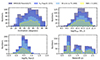 |
Fig. 1. Distributions of the physical properties of the KMOS3D parent and selected sample, arranged from top-left to bottom-right: inclinations, stellar masses, effective radii, and redshifts. The dark blue histogram represents all Hα datacubes with confirmed spectroscopic redshift. The blue histogram shows Hα-detected galaxies with Flag-0 or Flag-1 in Table-6 of Wisnioski et al. (2019). We further select galaxies with inclination angles between 25° ≤θi ≤ 75°, shown in the sky-blue histogram. Lastly, we narrow our focus to galaxies with a signal-to-noise ratio greater than 3, depicted by the yellow hatched histogram. This selection criteria allowed us to perform the robust kinematic modeling of these high-z galaxies. |
2.2. KGES
The KGES encompasses a sample of 285 galaxies located in the COSMOS, CDFS, and UDS fields, with redshifts ranging from 1.2 to 1.9 (Tiley et al. 2021). The survey primarily targets the Hα, [NII]6548, and [NII]6583 emission lines, which are redshifted to the H-band wavelength range (approximately 1.46 − 1.85 μm). For the current study, we focus on the subset of 225 KGES star-forming galaxies with confirmed spectroscopic redshifts, Hα detection, and not flagged as AGNs. Additionally, we restrict our analysis to galaxies with a K-band magnitude of K< 22.5, similar to Gillman et al. (2020). The median redshift of our sample is z = 1.49 ± 0.07, and the median seeing (FWHM) in the H-band observations is 0.7″. The aperture size of the Hα cubes is 1.2″ in radius, same as the KROSS Hα cubes discussed below in Section 2.3.
Physical properties of galaxies: The physical properties of the KGES sample can be found in Tiley et al. (2019a), Gillman et al. (2020) and Tiley et al. (2021). In particular, stellar masses were estimated by fitting the SED of galaxies using a routine called Multi-wavelength Analysis of Galaxy Physical Properties (MAGPHYS; da Cunha et al. 2008). The SED of each galaxy was constructed using multi-wavelength photometry ranging from the ultraviolet to the mid-infrared. The MAGPHYS routine compares the observed SEDs with the SEDs from the spectral libraries of Bruzual & Charlot (2003), includes the dust attenuation model of Charlot & Fall (2000), continuous star-formation histories, and Chabrier (2003) IMF. The resulting stellar mass range of the Hα-detected sample is 8.62 ≤ log(Mstar [M⊙])≤11.66, as reported in Tiley et al. (2021). Star formation rates and its uncertainties were estimated from the Hα flux, corrected for dust attenuation, assuming a Calzetti et al. (1994) extinction law. The estimated star formation rates range from 0.0 ≤ log(SFR [M⊙ yr−1])≤2.2. Similar to KMOS3D, the statistical uncertainty on stellar masses and star-formation rates is assumed to be 10%. Additionally, we add systematic uncertainty of 0.14 dex on stellar mass and 0.25 dex on star-formation rate. Geometrical parameters such as the effective radius, inclination, position angle, and central x-y coordinates were derived using the GALFIT (Peng et al. 2010). For detailed calculations of all physical quantities, we refer the reader to Gillman et al. (2020).
Primary selection criteria: To ensure the quality of datacubes and robustness of our kinematic modeling, we employ the identical selection criteria that were chosen for KMOS3D (as established in Sharma et al. 2021a). Firstly, we select galaxies with confirmed spectroscopic redshifts detected in Hα. Subsequently, we narrow down the sample based on two additional criteria: a) high inclination angle (25° ≤θi ≤ 75°) and b) S/N > 3. By applying these selection criteria, we are left with a set of 51 galaxies with sufficiently high S/N, which enables us to conduct accurate kinematic modeling. Figure 2 presents the distributions of physical properties of KGES selected sample, same as in Figure 1 which is for the KMOS3D sample.
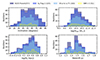 |
Fig. 2. Distributions of the physical properties of the KGES parent and selected samples, arranged from top-left to bottom-right: inclinations, stellar masses, effective radii, and redshifts. The dark blue histogram represents all Hα datacubes with confirmed spectroscopic redshift. The blue histogram shows Hα-detected galaxies (Tiley et al. 2021). We further select galaxies with inclination angles between 25° ≤θi ≤ 75°, which are shown in the sky-blue histogram. Lastly, we narrow our focus to galaxies with a signal-to-noise ratio greater than 3, depicted by the yellow hatched histogram. This selection criteria allowed us to perform the robust kinematic modeling of these high-z galaxies. |
2.3. KROSS
Additionally, we use the KROSS dataset (Stott et al. 2016), which was previously studied in Sharma et al. (2021a,b) and Sharma et al. (2022) (and also by Harrison et al. 2017; Johnson et al. 2018; Tiley et al. 2019b). The KROSS targets are selected from extragalactic deep fields covered by multi-wavelength photometric and spectroscopic data: (1) Extended Chandra Deep Field Survey (E-CDFS: Giacconi et al. 2001; Lehmer et al. 2005), (2) Cosmic Evolution Survey (COSMOS: Scoville et al. 2007), (3) Ultra-Deep Survey (UKIDSS: Lawrence et al. 2007), and (4) SA22 field (Steidel et al. 1998). Some of the targets were also selected from the CF-HiZELS survey (Sobral et al. 2015). The targets were selected such that the Hα emission is shifted into J-band with a median seeing of 0.7″. The aperture size of the Hα cubes is 1.2″ in radius. The KROSS sample studied in Sharma et al. contains 225 galaxies with redshift 0.7 ≤ z ≤ 1.04, inclination range 25° < θi ≤ 75°, effective radius 0.08 ≤ log(Re [kpc])≤0.89, stellar mass 9.0 ≤ log(M* [M⊙]) < 11.0, and circular velocity 1.45 ≤ log(Vout [km s−1])≤2.83, where Vout is calculated at Rout = 2.95Re.
2.4. Estimating gas masses
Observations show that typical star-forming galaxies lie on a relatively tight, almost linear, redshift-dependent relation between their stellar mass and star formation rate, the so-called main sequence of star formation (MS; e.g., Noeske et al. 2007; Whitaker et al. 2012; Speagle et al. 2014). Most stars since z ∼ 2.5 were formed on and around this MS (e.g., Rodighiero et al. 2011), and galaxies that constitute it, usually exhibit a rotating disk morphology (e.g., Förster Schreiber et al. 2006; Daddi et al. 2010; Wuyts et al. 2011).
Figure 3 shows the position of the final sample (detailed in Section 3.4) with respect to the main sequence of typical star-forming galaxies (MS), i.e., their offset from the main sequence:
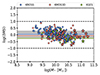 |
Fig. 3. Position of galaxies (final sample) with respect to the star-forming main sequence (MS). We plot offset from the MS, δMS (=SFR/SFR(MS; z, Mstar)) as a function of the stellar mass (Mstar) with the reference SFR(MS; z, Mstar) from Speagle et al. (2014). The gray shaded area represents the typical limit (0.3 dex) of star-forming MS (e.g., see Rodighiero et al. 2011; Genzel et al. 2015; Tacconi et al. 2018; Freundlich et al. 2019). The KMOS3D, KGES, and KROSS data are denoted by red, green, and blue filled circles, respectively. The solid lines in corresponding colors depict the average offset from the main sequence for each dataset. All galaxies are within 2σ scatter of the MS line. The galaxies marked with stars are the galaxies that have Re > PSF. |

where SFR(MS; z, Mstar) is the analytical prescription for the center of the MS as a function of redshift and stellar mass proposed in the compilation by Speagle et al. (2014), as a function of stellar mass. This figure shows that 64% of the galaxies in the total sample are within 1σ of the main sequence scatter, whereas the remaining 36% are within the 2 − 3σ range.
This enables us to estimate their molecular gas masses (MH2) using the Tacconi et al. (2018) scaling relations, which provide a parameterization of the molecular gas mass as a function of redshift, stellar mass, and offset from the MS stemming from a large sample of about 1400 sources on and around the MS in the range z = 0 − 4.5 (see also Genzel et al. 2015 and Freundlich et al. 2019). The scatter around these molecular gas scaling relations and the stellar mass induces a 0.3 dex uncertainty in the molecular gas mass estimates, which is accounted in the error estimates. The H2 mass of our sample is 9.48 ≤ log(MH2 [M⊙]) ≤ 11.03, with an average molecular gas fractions (fH2) of 0.21 ± 0.09, 0.14 ± 0.05, and 0.22 ± 0.06 for the KMOS3D, KGES, and KROSS sub-samples, respectively4.
To calculate the atomic mass (MHI) content of galaxies within the redshift range 0.6 ≤ z ≤ 1.04, we use the HI scaling relation presented by Chowdhury et al. (2022), which provides the first Mstar − MHI relation at z ≈ 1, encompassing 11,419 star-forming galaxies. The relation was derived using a stacking analysis across three stellar mass bins, each bin with a 4σ detection and an average uncertainty of ∼0.3 dex. This uncertainty in the gas scaling relation is additionally accounted in the error of HI mass estimates. To compute the HI mass at z > 1.04, we employ the Mstar − MHI scaling relation derived from a galaxy formation model under the ΛCDM framework (for details, see Lagos et al. 2011). This scaling relation successfully reproduces both the HI mass functions (Zwaan et al. 2005; Martin et al. 2010) and the 12CO luminosity functions (Boselli et al. 2002; Keres et al. 2003) at z ≈ 0 with an uncertainty of around 0.25 dex, as well as follows the observations of quasars from z = 0 − 6.4 (see Lagos et al. 2011, Fig. 12). The HI Mass range of our sample is 9.90 ≤ log(MHI [M⊙]) ≤ 11.42, with an average atomic gas fractions (fHI) of 0.42 ± 0.16, 0.48 ± 0.17, and 0.37 ± 0.06 for the KMOS3D, KGES, and KROSS sub-samples, respectively.
3. Forward modeling of the datacubes
We conduct a comprehensive reanalysis of the entire KMOS3D, KGES, and KROSS datasets, using the 3D forward modeling approach implemented by 3DBAROLO. In order to obtain precise kinematics, we used an optimization function in conjunction with 3DBAROLO to more accurately constrain the essential gas geometrical parameters (see Section 3.1). We found that galaxies with low S/N and a large PSF present a challenge in terms of accurate kinematic modeling. The former is related to the intrinsic brightness of the source, its distance, and the integration time of the observations; the latter to the intrinsic size and atmospheric conditions during observations, which can significantly degrade the resolution. Consequently, we had to discard the low S/N (∼3 − 5) and a large PSF (PSF ≥ Rmax of rotation curve) galaxies from the final analysis (see Section 3.2). Our final sample consists of 73 KMOS3D, 21 KGES, and 169 KROSS galaxies, i.e., a total of 263 objects (see the following subsections). The distributions of the physical properties of the final sample is shown in Figure 4.
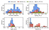 |
Fig. 4. Distributions of the physical properties of galaxies after kinematic modeling, arranged from top-left to bottom-right: inclinations, stellar masses, effective radii, and redshifts. These distributions are presented for the KMOS3D (in red), KGES (in green), and KROSS (in blue) samples. In total, we use 73 KMOS3D, 21 KGES, and 169 KROSS galaxies to estimate the DM fraction at high-z. The distribution of Re > PSF galaxies (within final sample) is shown by black hatched histograms. For detailed information on sample selection following kinematic modeling, we refer the reader to Section 3.2. |
3.1. Kinematic modeling
We modeled the kinematics of the galaxies in our samples using the 3DBAROLO code (Teodoro & Fraternali 2015). The main advantages of modeling datacubes with 3DBAROLO (hereafter 3DBarolo) are that (1) it allows us to reconstruct the intrinsic kinematics in three spatial and three velocity components for given initial guesses that define the kinematics and geometry of a galaxy; (2) the 3D projected modeled datacubes are compared to the observed datacubes in 3D space; (3) it simultaneously incorporates instrumental and observational uncertainties (e.g., spectral smearing and beam smearing) in 3D space5. For details, we refer the reader to Teodoro & Fraternali (2015) and Di Teodoro et al. (2016). This three-fold approach of deriving kinematics is designed to overcome the observational and instrumental effects and hence allowed us to stay close to the realistic conditions of the galaxy. Therefore, it provides somewhat improved results compared to the 2D approach6, specifically in the case of small angular sizes and the moderate S/N of high-z galaxies (see Di Teodoro et al. 2016). Basic assumptions under 3DBarolo, its basic requirement, and limitations are detailed in Sharma et al. (2021a, Section 3.1) and briefly mentioned below.
The kinematic modeling with 3DBarolo requires three geometrical parameters – namely the galaxy’s central position (xc, yc), the inclination angle (θi), and the position angle (PA) –, and three kinematic parameters – namely the redshift (z), the rotation velocity (Vrot), and the velocity dispersion of the ionized gas (Vdisp). In our modeling, we set the geometrical parameters and redshift, while kinematic parameters are left free. 3DBarolo comes with several useful features particularly useful for high-z low S/N data7. We used 3DFIT TASK for performing the kinematic modeling. 3DBarolo produces mock observations given the input parameters in the 3D observational space (x, y, λ), where (x, y) stands for the spatial axes and λ is the spectral axis coordinate, resulting in a datacube: f(x, y, λ). These models were fit ring by ring to the observed datacube in the same 3D space, accounting for beam smearing. A successful run of 3DBarolo delivers the beam smearing corrected velocity (or moment) maps, the stellar surface brightness profile, the RC, and the dispersion curve along with the kinematic models. We note, the RC (or PV diagrams) are not derived from the velocity maps, but instead calculated directly from the datacubes by minimizing the difference in VLOS = Vrot sin θi of model and data in each ring.
When we employed 3DBarolo to model the galaxies, we discovered that the photometric geometrical parameters (xc, yc, and PA) were inadequate for accurately representing (or extracting) their kinematics. This inadequacy arises because gas kinematics differ from stellar kinematics due to their distinct morphologies (i.e., geometry) and alignments. In particular, as we go higher in redshift, gas morphological parameters (PA, xc, and yc) start differing from their photometric measurements, i.e., stellar morphology (as reported in Wisnioski et al. 2015; Harrison et al. 2017; Sharma et al. 2021a). Moreover, from our previous work with 3DBarolo (Sharma et al. 2021a), we also learned that 3DFIT TASK is incapable to constrain simultaneously multiple (more than 2) parameters, most likely due to low quality data at high-z8.
Therefore, in this work, we estimated the gas geometrical parameters using an optimization function that runs atop 3DBarolo, namely minimizing the following loss function:
![$$ \begin{aligned} \ell = \sqrt{ \overline{(X_D - X_M)^2} } + \frac{N[D]}{N[D: \ne 0, \ne \pm \infty ]} + \frac{N[M]}{N[M: \ne 0, \ne \pm \infty ]}, \end{aligned} $$](/articles/aa/full_html/2025/07/aa47922-23/aa47922-23-eq3.gif)
where XD/M is an array of data or a model, N represents the length of the array, and D and M stand for data and model, respectively. In the equation, the first term corresponds to the root mean square error, the other two terms are the weights of the data and the model. In the denominators, N[D : ≠0, ≠ ± ∞] gives the length of the datacube which includes only non-zeros and finite elements; N[M : ≠0, ≠ ± ∞] gives the same for the model. That is, weights are higher if the datacube contains more zero or infinite elements; in which case, the loss function (ℓ) is higher. We use a Nelder-Mead minimization method9, which is available in the scipy.optimize library. This optimization function enables to fit multiple parameters with 3DBarolo. We ran 3DBarolo on each object as we did in Sharma et al. (2021a), i.e., the free parameters in 3DBarolo are only Vrot, Vdisp and the extra parameters are constrained by the optimizer. The details of the logical flow of optimization with 3DBarolo are described in Appendix B.
3.2. Inspection of kinematic modeling outputs
We modeled the kinematics of 541 star-forming galaxies: 265 from KMOS3D, 51 from KGES, and 225 from KROSS. For quality assessment and assurance, we inspected the outputs of 3DBarolo+optimization for each individual galaxy. Firstly, we scrutinized the optimization log of all KMOS3D and KGES galaxies. In KMOS3D, we notice that, 57 of them experienced optimization failure due to quality of observations or inaccurate parameters such as PA, xc, yc (see discussion in Appendix B). Secondly, 3DBarolo could not perform the modeling on 52 galaxies owing to their large PSF (i.e., Rmax≤ PSF, where Rmax is the maximum radius of the rotation curve). Furthermore, we observed that 78 galaxies had a maximum radius comparable to the PSF, thereby allowing 3DBarolo to form only two rings, the first of which being unreliable (see Di Teodoro et al. 2016 and Sharma et al. 2021a). Consequently, rotation curves obtained from these galaxies cannot be used in dark matter fraction studies. Lastly, we inspected the velocity maps and high-resolution photometric images, and we noticed that five galaxies have disturbed kinematics due to nearby neighbors, and therefore we discarded them. After kinematic modeling, in total, we had to exclude 192 objects. It is not surprising for us to lose a lot of high-z data, as these observations are often noisy and the angular size of the objects very small. This is consistent with the findings of previous studies on KMOS3D data, which were often conducted on a relatively small sub-sample (see, Genzel et al. 2017, 2020, and references therein). The final KMOS3D sample contains 73 galaxies, which is still large enough to perform a statistical study.
Within the KGES dataset, three galaxies encountered optimization failures, while 11 galaxies exhibited a larger PSF compared to the actual galaxy size. Additionally, 16 galaxies displayed a maximum radius that was comparable to the PSF, thereby allowing 3DBarolo to form only two rings, the first of which being unreliable. Consequently, these galaxies were deemed unsuitable and were excluded from further analysis. As a result, our final KGES sample contains only 21 galaxies. Furthermore, for the details of comparison sample, i.e., KROSS objects, see Appendix B. In the end, we retain 263 galaxies, 73 from KMOS3D, 21 from KGES, and 169 from KROSS.
3.3. Kinematic modeling results
Figure 5 shows a few examples of the kinematic modeling results. In this figure, the first three columns in each row show the moment maps10, data, model, and residuals, respectively, from left to right. As we can see, model closely matches the data, and residuals lie around (below) 5% of the total velocity. However, we do notice slight structures in the residual maps that could potentially be associated with irregular gas motions or turbulent flows, which were not accounted in 3DBarolo, one of the caveats (along with other ones) highlighted in Section 5. Nevertheless, these results represent the most optimal outcome achievable through the utilization of both 3DBarolo and the optimization function. The fourth column displays the major axis position-velocity diagram (PV diagram), which is the line-of-sight (LOS) rotation velocity of the galaxy at each spatial bin11. The red contour represents the model, and the black shaded area with blue contour represents the data. The orange squares with error bars indicate the best-fit LOS rotation velocity. The yellow and blue vertical dashed lines represent the effective radius (Re) and optical radius (Ropt = 1.89 Re) of the galaxy, respectively. The last column presents the velocity dispersion curve. The last column presents the velocity dispersion curve. We note that the first (inner) data point in the rotation curves and velocity dispersion profiles occasionally exhibits unexpectedly high or low values, a known issue with the 3DBarolo code (Di Teodoro et al. 2016; Sharma et al. 2021a), which most-likely arises due to limited resolution in the data. In our calculations, we discard this inner data point as it is irrelevant for science. However, we discuss (and present) it here to indicate the limitations of our kinematic modeling technique.
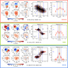 |
Fig. 5. Outputs of the kinematic modeling of selected KMOS3D (red box), KGES (green), and KROSS (blue) sources obtained using 3DBAROLO. Row-1, Columns 1-3: Rotation velocity map data, model, and residuals, respectively. The gray dashed line shows the position angle, the black cross the central x-y position, and the green line marks the plane of rotation. Row-2, Columns 1-3: Velocity dispersion map data, model, and residuals, respectively. Column 4: Major axis PV diagram, where the black shaded area with blue contour represents the data while the red contour shows the model, and the orange squares with error bars are the best-fit line-of-sight rotation velocity inferred by 3DBAROLO. The yellow and blue vertical dashed lines represent the effective radius (Re), and the optical radius (Ropt = 1.89 Re), respectively. Column 5: Corresponding velocity dispersion curve. The first point in the rotation and dispersion curves is represented by an empty (or white) marker, as it falls under the resolution limit and is therefore excluded from the data analysis. |
To estimate the DM fraction, we first correct the rotation curves for pressure support, as the turbulent interstellar medium in high-z galaxies makes them pressure-supported systems (Burkert et al. 2010; Übler et al. 2019). In Sharma et al. (2021a), it was demonstrated that high-z galaxies exhibit a non-uniform and non-isotropic velocity dispersion, inducing a pressure gradient. This pressure gradient significantly hampers the motion of gas, leading to a decrease in the rotation velocity of the gas in the inner region of galaxies by ∼50% of its original value. In some cases, it also affects the outer rotation curves, causing them to decline.
To address this issue, Sharma et al. (2021a) introduced a method known as the ‘pressure gradient correction’ (PGC), which effectively corrects for gas pressure. This approach is analogous to the ‘asymmetric drift correction,’ which addresses stellar pressure, as discussed in Sharma et al. (2021a, Sec. 3.2). In this study, we applied the PGC method to all datasets and investigated the impact of velocity dispersion on the circular velocity of galaxies. In Figure 6, we present the intrinsic velocities (Vint) and pressure-corrected circular velocities (VPGC) within Rout, color coded for intrinsic rotation-to-dispersion ratio ( ), where Vint is rotation velocity without pressure support corrections. As shown, systems primarily supported by rotation (
 ) exhibit minimal or no pressure correction, whereas dispersion-dominated systems induce significant correction. Additionally, there are substantial pressure corrections at the lower end of the velocity range (log(VRout[km/s]) < 2.3), that gradually decrease toward higher velocities and approaches zero. We note to the readers that, prior to the implementation of PGC, there were only 9 dispersion dominated galaxies (3 KMOS3D, 1 KGES, and 5 KROSS). However, after applying PGC, none of these galaxies have
  , as depicted in Figure B.4. Therefore, we do not exclude these galaxies from our analysis. Hence, the full sample is a good representative of rotation supported system.
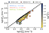 |
Fig. 6. Impact of the pressure gradient on the circular velocity of galaxies computed at Rout. The KMOS3D, KGES, and KROSS samples are denoted by red circles, green cross, and blue stars, respectively. The interior of each data point is color-coded for rotation-to-dispersion ratio computed before pressure support correction ( |

Finally, we examined the relationship between the size of the PSF and the effective radius and found that 59% (43) of KMOS3D, 90% (19) of KGES, and 88% (148) of KROSS galaxies possess a PSF larger than their effective radius, i.e., only 53 galaxies have Re > PSF as shown in Figure 7. This suggests that the majority of the sample cannot be used for studying the dark matter fraction within Re, as doing so would result in highly uncertain outcomes. Hence, we only used the 53 galaxies with a large enough effective radius compared to the PSF to characterize the DM fraction within that effective radius. Additionally, 16% (12) of KMOS3D, 19% (4) of KGES, and 42% (71) of KROSS galaxies have a PSF larger than their optical radius. However, only 1.4% (1) of KMOS3D, 0.0% (0) of KGES, and 12% (20) of KROSS galaxies have a PSF larger than their outer radius. Therefore, the most reliable measurement of the dark matter fraction is obtained within the outer radius (Rout). Consequently, in this work we mostly focus on interpreting the results that are computed within (or at) Rout.
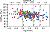 |
Fig. 7. Stellar masses as a function of ratio between PSF/Re. The KMOS3D, KGES, and KROSS samples are represented by red circles, green crosses, and blue stars, respectively, with a vertical dashed line indicating PSF = xRe. This figure indicates that only a limited number (= 53) of galaxies are applicable for determining the dark matter fraction within Re. However, it is important to note that our analysis is not restricted within Re. In fact, we evaluate the dark matter fraction at outer radii (i.e., R > Re). |
It is important to note that about 83% and 67% of the galaxy rotation curves extend to Ropt and Rout, respectively. As shown in Figure 8, only 17% and 33% of galaxies have Ropt and Rout beyond the last observed radius (Rlast) in the rotation curves. For cases where the rotation curve does not reach the reference radius, we interpolate the velocity estimates. We did not assume any specific functional form for the rotation curve; instead, we used the numpy.interp routine, which applies linear interpolation. This approach ensures that if the rotation curve is declining, it will continue to decline, and vice versa. Our approach is as follows: if Ropt or Rout exceeds Rlast, we calculate fDM(< Rscale) at the nearest observed point. This method ensures that our analysis remains within the observed region of each galaxy.
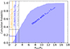 |
Fig. 8. Cumulative distribution of the ratio between the last observed radius in the rotation curves (Rlast) and the effective radius (Re). The yellow, blue, and gray dashed lines indicate the scale radii Re, Ropt, and Rout, respectively. This plot shows that for the entire sample, Rlast > Re, while approximately 83% and 67% of objects have Rlast greater than Ropt and Rout, respectively. |
Moreover, when the characteristic radii (Rout,RoptRe ) are not covered in the observed rotation curve, we impose additional uncertainties on the circular velocity (Vc) measurements at those radii to account for potential errors introduced by interpolation or extrapolation. Specifically, we increase the uncertainties by 10% when Vc is estimated at Rout or Ropt, and by 25% when evaluated at Re. The smaller penalty at Rout and Ropt is motivated by the fact that they lie in the outskirts where rotation curves are relatively flat; hence, interpolation is less prone to large deviations. In contrast, the inner regions within Re often exhibit steeper velocity gradients, justifying a more conservative error adjustments.
3.4. Final sample
To summarize the sample selection, it is crucial to note that the initial selection of galaxies for kinematic modeling was based on the following criteria: (1) confirmed Hα detection and spectroscopic redshift, (2) inclination angles within the range of 25° ≤θi ≤ 75°, and (3) S/N > 3. This primary selection criteria is detailed in Section 2 for the KMOS3D and KGES datasets and outlined in Table 1. Following the primary selection criteria, our chosen sample comprises 265 KMOS3D galaxies and 51 KGES objects, as depicted in Figure 1 and Figure 2. For the KROSS dataset, we utilized the complete set of 256 galaxies analyzed in Sharma et al. (2021a).
Primary and secondary sample selection criteria.
Following the kinematic modeling process (Section 3), we implemented secondary selection criteria as detailed in Section 3.2 and outlined in Table 1. Under this criteria, galaxies were excluded if they met the following conditions: (1) 3DBarolo+ optimization did not succeed, indicating unreliable optimized parameters such as PA or central coordinates; (2) No mask was created, implying 3DBarolo’s failure to mask true emission due to moderate signal-to-noise; (3) Rmax < PSF, indicating 3DBarolo’s inability to create rings and hence fails to produce kinematic models; (4) Rmax = PSF, in this case resulting kinematic models provide only two measurements in rotation curves, which were insufficient for dynamical modeling. This secondary selection criteria resulted in a final sample of 263 galaxies, comprising 169 from KROSS, 73 from KMOS3D, and 21 from KGES. The distribution of relevant physical quantities for the final sample across all datasets is presented in Figure 4, and their location with respect to star-forming galaxies is shown in Figure 3.
In addition, we emphasize to the reader that the computation of the dark matter fraction within Re was exclusively performed on 53 galaxies having Re > PSF, as depicted in Figure 7 and discussed in Section 3.3. These 53 objects are also highlighted separately in the Figure 3 and Figure 4. However, the goal of this work is to go beyond the specific case of the ‘dark matter fraction within Re’. As elaborated in Section 4, we present the dark matter fraction and scaling relations at outer radii (R > Re, where R is the running radius of rotation curve) using the full sample of 263 galaxies. Furthermore, we note that the maximum radius (Rmax or Rlast) of galaxies in the final sample is larger than the PSF, see Figure B.3, i.e., this sample is suitable for estimating dark matter at outer radii.
4. Results
Our primary goal is to measure the dark matter fraction across various galactic scales. Recent studies at high-z suggest that galaxies contain baryon-dominant inner regions (within Re), where dark matter constitutes less than 20% of the total mass (Genzel et al. 2020; Nestor Shachar et al. 2023). Adding to this perspective, a study by Lelli et al. (2023) found that the kinematics of two main-sequence galaxies, from the cosmic dawn, could be entirely explained by baryon only dynamical models, eliminating the need for dark matter. These findings amplify the long-standing disk-halo degeneracy issue, a challenge that persists even in local galaxies (van Albada et al. 1985), and remains unresolved, particularly when mass-to-light ratios are not entirely reliable (Sofue & Rubin 2001; Bullock & Boylan-Kolchin 2017). Therefore, in this work, we adopt a conservative approach, beginning with the mass-modeling of rotation curves under the conditions of maximal baryonic disk, using the Bayesian inference technique established in Sharma et al. (2022, Sec. 3.1). We assumed that stars and gas follow an exponential distribution (Freeman 1970) such that the mass-modeled rotation curve of a galaxy is given by
![$$ \begin{aligned} V_{\_}^2(R) = \frac{1}{2} \Big ( \frac{GM_{\_}}{R_{\rm scale}} \Big ) \ \Big ( \alpha \frac{R}{R_{\rm scale}} \Big )^2 \ [I_0K_0 - I_1K_1], \end{aligned} $$](/articles/aa/full_html/2025/07/aa47922-23/aa47922-23-eq8.gif)
where M_ and Rscale are the total mass and the scale length of the different components (stars, H2, and HI), respectively, and In and Kn are modified Bessel functions computed at α = 1.6 for stars and α = 0.53 for gas (cf. Persic et al. 1996; Karukes & Salucci 2017).
We mass-modeled the rotation curves under two scenarios that consider the maximum contribution from (1) the stellar disk, i.e., M_ = Mstar, and (2) baryonic (stars+gas) disk, i.e., M_ = Mstar + (1.33 * MHI)+MH2, details are compiled in Appendix C. Figures B.5 and B.6 provide a few examples of mass-modeled RCs. We compare these rotation curves with their fiducial (fid) values, i.e., velocity profile derived directly from the photometric stellar and gas masses discussed in Section 2.4. In Figure 9, we present a comparison between the fiducial (i.e., masses from photometry) and the mass-modeled stellar and baryonic masses in the case of maximum stellar disk and maximum baryonic disk scenarios (upper and lower panels, respectively). When considering the maximum stellar disk, we observed that fitting the rotation curves requires stellar masses that are twice the values obtained from photometric measurements for the majority of the sample. This finding strongly suggests the requirement of an additional gas component at high-z, which we incorporate in the maximum baryonic disk scenario. However, as illustrated in the bottom panel of Figure 9, even after including the gas component, more than 50% of the sample still demands baryonic masses that are a factor of two higher than their fiducial values. Such values are unrealistic to obtain within the range of observed uncertainties. That is, with a large sample of 263 galaxies, we are unable to rule out the presence of dark matter halos at high-z.
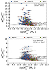 |
Fig. 9. Comparison of photometric (PHOT) stellar and baryonic (stars+gas) masses with mass-modeled stellar and baryonic masses in the case of the maximum stellar disk and maximum stellar+gas disk scenarios, upper and lower panels, respectively. The KMOS3D, KGES, and KROSS datasets are depicted in red, green, and blue colors, respectively. The dashed black line indicates when mass-modeled masses are equivalent to their fiducial values (i.e., photometric masses), suggesting that objects lying above this line require the presence of a dark matter halo. |
Moreover, recent observations of high-z galaxies suggest that longer integration time is crucial for accurately mapping the complete kinematics. In particular, a work by Puglisi et al. (2023) on KMOS Ultra-deep Rotation Velocity Survey (KURVS) has demonstrated that deep observations enhance both the amplitude and radial extent of the rotation curves. Consequently, deep observations of our current sample will further demand the inclusion of an additional halo component, as anticipated while analyzing the mass-modeled rotation curves (see Figure B.6). Additionally, the Freeman model assumes a razor-thin disk, which is an extreme case. Allowing for a finite thickness of the disk would further decrease the circular velocity of the baryonic component and will provide the more room for the dark matter. Henceforth, we proceed the investigation of the rotation curves in the presence of a dark matter halo component.
The total dark matter mass can be calculated by subtracting the baryonic mass contribution from observed rotation curve, (V2(R)−Vbar2(R) = GMDM/R) as a function of radius, as explained in Appendix C. That is, dark matter halo modeling is not necessary to study the amount of dark matter. In order to estimate the dark matter fraction of our datasets, we used Equation (D.3), which is a halo model independent approach (previously postulated in Sharma et al. 2021b), yet it allowed us to estimate the dark matter at different galactic scales. We estimated the uncertainties in the dark matter fraction using Monte Carlo sampling, propagating the errors in velocity and mass estimates throughout the analysis. We begin by inspecting dark matter fraction within Re, which is a rather controversial issue for high-z galaxies. For example, Genzel et al. (2020) and Nestor Shachar et al. (2023) reports dark matter-deficiency within Re at high-z, on the other hand, Sharma et al. (2021b) and Bouché et al. (2022) reported a similar amount (> 45%) of dark matter fraction as seen in local star-forming disk galaxies.
4.1. Dark matter fraction within Re
Here, we present the dark matter fraction only for the galaxies that have Re > PSF. In total, we have only 20% (53) galaxies that abide this criteria, and cover the redshift range of 0.73 ≤ z ≤ 2.43. 12 The results are shown in Figure 10. We observe that six galaxies fall in the ‘forbidden’ region, where Mdyn < Mbar, possibly indicating inaccurate photometric stellar mass estimates or incomplete sampling of stellar and gas motion in the observed rotation curves. However, we do expect some data points with low dark matter fraction to fall within this region given the uncertainties on the measurements of stellar masses and SFRs. Apart from forbidden region galaxies, ∼8 galaxies exhibit dark matter deficiency within Re (fDM < 20%). Notably, the dark matter fraction of very massive (> 1010.5 M⊙) galaxies in our sample surpasses that of local massive galaxies, such as the Milky Way (Petač 2020, and ref. therein) and Andromeda galaxies (Tamm et al. 2012, and ref. therein), represented by blue and orange stars in Figure 10, respectively.
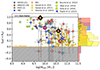 |
Fig. 10. Dark matter fraction within Re as a function of stellar masses for galaxies having Re > PSF. The KMOS3D, KGES, and KROSS datasets are depicted in red, green, and blue colors, respectively. The errors on the datasets are 68% confidence intervals. For comparison, we include two local massive disk galaxies: the Milky Way (MW) and Andromeda (M31), represented by the blue and the orange star, respectively. Additionally, we compare these results with previous studies at high redshift, such as Genzel et al. (2017, yellow circles), Genzel et al. (2020, yellow hexagons), Nestor Shachar et al. (2023, yellow dots), Bouché et al. (2022, yellow star), Übler et al. (2018, yellow diamond), Drew et al. (2018, yellow cross), and Puglisi et al. (2023, purple triangle). The black square represents the two galaxies that are in-common with Genzel et al. (2020) drawn from this work, while pink hexagons shows the measurements of same objects from Genzel et al. (2020). The black and yellow horizontal dashed lines represent the regimes of 100% dark matter dominance and baryon dominance, respectively. The gray shaded area indicates the ‘forbidden’ region, where galaxies with Mdyn < Mbar are located. Horizontal histograms (aligned to the right y-axis) compare datasets: KMOS3D, KGES, and KROSS (filled red, green, and blue hists), Genzel et al. (2017, 2020) (yellow fill with solid brown line), Nestor Shachar et al. (2023) (yellow fill with dashed brown line), and Bouché et al. (2022) and Puglisi et al. (2023) (open histograms in green and purple, respectively). |
We compared our findings with those of previous studies, such as Genzel et al. (2017), Übler et al. (2018), Drew et al. (2018), Genzel et al. (2020), Nestor Shachar et al. (2023), Bouché et al. (2022), and Puglisi et al. (2023), as shown by the different markers in Figure 10. Our results are in full agreement with Bouché et al. (2022), Drew et al. (2018), and a few galaxies of Genzel et al. (2020), Nestor Shachar et al. (2023) and Puglisi et al. (2023). However, we observe that the majority of Nestor Shachar et al. (2023), Genzel et al. (2020), and Genzel et al. (2017) are baryon-dominated, including a galaxy of Übler et al. (2018). Specifically, the very massive galaxies studied in Genzel et al. (2020) and Nestor Shachar et al. (2023) are dark matter deficient, which contrasts with our findings, where majority of galaxies in the same mass range have ∼30%−58% dark matter, except two. However, we cannot draw any concrete conclusions due to the limited number of data points and their large uncertainties. Nevertheless, to aid the reader and facilitate a visual comparison between studies, we include horizontal histograms corresponding to each dataset along the y-axis of Figure 10, illustrating the degree of agreement or discrepancy.
Next, we cross-matched KMOS3D sample and the galaxies studied in Genzel et al. (2020), resulting in the identification of only two overlapping systems: GS4_05881 (z = 0.99) and GS4_43501 (z = 1.61). These systems are represented by black squares in Figure 10. According to Genzel et al. (2020), the reported dark matter fractions within Re for these two systems are fDM(< Re) = 0.64 and 0.19, respectively, shown by pink hexagons. While our estimates are about 0.98 and 0.55, respectively, i.e. ∼1.5 and 3 times higher than the estimates reported in Genzel et al. (2020). This difference is most likely attributed to the distinct kinematic modeling and pressure support corrections implemented in this work, quantified and reported previously in Sharma et al. (2021a,b). Moreover, it is noticeable that the stellar masses of these objects reported in Genzel et al. (2020) are marginally higher than those in the present study. This discrepancy arises because we employ photometric stellar masses, whereas Genzel et al. (2020) utilizes dynamically mass-modeled (best-fit) stellar masses.
Furthermore, we had the opportunity to refine the measurement of Re for a subset of the KROSS sample through the latest observations from the James Webb Space Telescope (JWST). This particular subset of galaxies is situated within the COSMOS field (Skelton et al. 2014), which has recently undergone observation by the COSMOS-WEB team (Casey et al. 2023). Estimates of Re for these galaxies were derived using GALFITM (Häußler et al. 2013) setup equal to that presented in Martorano et al. (2023). As discussed in Appendix E and illustrated in Figure E.2, we observe that the new Re estimates shift the galaxies of low dark matter fractions (< 20%) toward higher values. In this specific sub-sample, majority ( 95%) of the galaxies have a dark matter fraction above 20%. Consequently, we suggest that a low (< 0.2) dark matter fraction within Re is possible for massive disk-like galaxies at high redshifts (0.65 ≤ z ≤ 2.2), but it is very unlikely for all mass ranges (8.5 ≤ log(M* [M⊙]) ≤ 10.5).
4.2. Dark matter fraction within Rout
In Figure 11, we plot the dark matter fraction within Rout ( = 2.95 × Re), as a function of stellar mass. Firstly, we observe that the 47% of the sample exhibits dark matter-dominated outer disks, with 23% of objects showing 0.2 ≤ fDM(< Rout) < 0.5, and 28% of objects having fDM(< Rout) < 0.2 (including objects in the forbidden region). Secondly, we notice a slightly decreasing trend of fDM as a function of stellar mass, excluding a few outliers. These outliers are six massive galaxies in the KMOS3D sample that display prominent disks in HST images and exhibit rising-flat rotation curves, as shown in Figure E.313. Notably, their dark matter halos are as massive as those of the most massive systems in the present-day Universe, such as the Milky Way (MW) and Andromeda (M31), shown by blue and orange stars, respectively, in Figure 11.
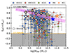 |
Fig. 11. Dark matter fraction within Rout. The KMOS3D, KGES, and KROSS datasets are represented in red, green, and blue colors, respectively. The binned dark matter fraction, calculated using weighted mean and root-mean-square statistics discussed in Section 4.2, is represented by off-white and white color hexagons, respectively, connected by black lines. The uncertainties on individual and binned data points represent the 68% confidence interval. For comparison, we include two local massive disk galaxies: the Milky Way (MW) and Andromeda (M31), represented by the blue and the orange star, respectively. The pink shaded area represents local star-forming disks (Persic et al. 1996). The solid black dashed line represents the 100% dark matter regime, while the yellow dashed line represents the baryon-dominated regime. The gray shaded area indicates the ‘forbidden’ region, where galaxies with Mdyn < Mbar are located. These color codes are same throughout the text. |
To compare these measurements with local star-forming galaxies (SFGs) (Persic et al. 1996), we average the dark matter fraction, fDM(<Rout), across five stellar mass bins, excluding the massive galaxies (log(Mstar/M⊙) > 10.5). Recalling Sharma et al. (2021b), authors estimated the dark matter fraction using the same method as in this work. However, the uncertainties were propagated using the python-uncertainty package without accounting for systematics in stellar masses, star formation rates, and gas masses, resulting in relatively small uncertainties. Therefore, simple root-mean-square statistics was used to compute the average values and errors (for details, see Sharma et al. 2021b). The resulted dark matter fractions agreed with local studies. In this work, applying the same statistics results in 20% low dark matter fraction compared to local studies as shown by white hexagons in Figure 11.
We remark that in this work, we estimated the uncertainties by accounting for both statistical and systematic uncertainties in stellar masses and star formation rates (SFRs), as well as the scatter in gas mass scaling relations (see Sections 2.1 & 2.2). These uncertainties are propagated throughout the analysis using Monte Carlo sampling with 10 000 samples. This procedure leads to more reliable results, albeit at the cost of significantly larger uncertainties on individual data points. Consequently, the conventional binning method (as employed in Sharma et al. 2021b) used to average out the dark matter fraction likely underestimates its values. Therefore, we also applied weighted-mean statistics, given by  , where,
  . This binning technique assigns greater influence to data points with higher precision by weighting the errors during averaging. The uncertainties on the binned data points are estimated using bootstrap resampling. As shown by off-white hexagons in Figure 11, the binned dark matter fraction within Rout matches the local studies. Additionally, we observe a slightly declining trend as a function of stellar mass.
In Appendix E, Figure E.1 shows the results of dark matter fraction within Ropt ( = 1.89 × Re). We notice that dark matter fraction is on average 10% less within Ropt than Rout, suggesting that dark matter dominates the outer-disks at high-z, which is very similar to local disk galaxies (Persic et al. 1996). Finally, we investigate galaxies with fDM(< Rout) < 20% in relation to their PSF and S/N, but no dependencies are found.
To further investigate, we estimated the stellar masses (within scale radius, e.g., Rout) of these objects using the Sérsic profile. It is important to note that the stellar masses derived under the Freeman disk assumption are, on average, 1.02 times higher than those obtained using the Sérsic profile (see Appendix D and Figure D.1). In ideal cases where dark matter dominates, the dark matter fraction estimated using the Sérsic profile–assuming a Sérsic index of n = 1−1.35–is only ∼2% higher. However, significant changes arise when the stellar or gas mass constitutes a substantially larger fraction of the total mass, typically by 0.7–1 dex (i.e., a factor of five to ten), as observed in galaxies with low dark matter fractions in our sample. Furthermore, assuming a Sérsic index of n > 1.5 implies that galaxies are more dark matter dominated in the outskirts while being baryon-dominated in the inner regions. Consequently, modifying the assumed stellar mass profile can significantly increase the estimated dark matter fraction for systems that lie in the ‘forbidden’ region or exhibiting low fDM(<20%) within Rout. Since Sérsic indices for the full sample are not available and computing them is beyond the scope of this study, we adopt the Freeman disk profile throughout. This choice is motivated by the fact that galaxies in our sample are predominantly disky morphology seen in the high-resolution images. Nevertheless, we acknowledge the importance of further investigating the role of galaxy morphology and structural parameters in shaping the inferred dark matter fraction.
4.3. Dark matter fraction across cosmic time
To gain a deeper understanding of the evolution of dark matter with cosmic time, we initially divided the dark matter fraction, fDM(< Rout), into three redshift bins: 0.5 < z ≤ 1.1, 1.1 < z ≤ 1.8, and 1.8 < z ≤ 2.5. We employed weighted mean statistics to determine the binned values, and the errors were estimated using a bootstrap method as explained in Section 4.2. We note that during binning, we use only resolved galaxies with fDM(< Rout) > 0. The results are presented in Figure 12 (left panel), where the binned data points are denoted by large gray stars connected by a solid black line. Upon inspecting the figure, it becomes evident that the dark matter fraction exhibits a decreasing trend within the redshift range of 0.85 ≤ z ≤ 1.8. To confidently establish this trend beyond z > 1.8, additional data is required. Consequently, we refrain from further discussing the higher-redshift bin (z > 1.8) in our analysis.
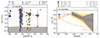 |
Fig. 12. Dark matter fraction across the cosmic time. Left panel: Dark matter fraction within Rout as a function of redshift. The color codes of datasets are same as Figure 11, and given in the legend of the plot. The gray stars represents the binned data points with 1σ uncertainty shown by error-bars. Right panel: Averaged dark matter fraction within Re, Ropt, and Rout as a function of redshift, represented by yellow and blue lines, respectively. The bootstrap-errors representing 68% confidence interval are indicated by shaded areas color-coded with the same color as the averaged line. Dark matter fraction of local star-forming galaxies within Ropt and Rout are from Persic et al. (1996), and within Re they are taken from disk galaxy survey of Courteau & Dutton (2015). The uncertainties on these measurements are, on average, ±0.25. The color code of these estimates are same as high-z galaxies. The dark-yellow dotted-dashed lines shows the dark matter fraction within Re from Nestor Shachar et al. (2023). |
In the right panel of Figure 12, we present the binned dark matter fraction within Re, Rout, and Rout, as a function of redshift. We observe that the dark matter fraction increases on galactic scales as we move outward, from Ropt to Rout. We had anticipated that the dark matter fraction within Re would be lower than the Ropt and Rout. However, our findings show the contrary:  at z ∼ 1. This discrepancy could be real or an artifact caused by the very low number of resolved galaxies within Re. Nevertheless, at z ∼ 1 the difference in dark matter fraction at different radii is not significant, but it is certainly not declining rapidly. On an average, the dark matter fraction within the effective radius, at z = 1 − 1.8, does not go below 50%. These findings, especially, fDM(< Re) stand in contrast to those of Nestor Shachar et al. (2023), who reported a rapid decrease and low dark matter fraction within Re as a function of redshift. However, it is worth noting that in order to further refine our understanding on dark matter content within Re, more resolved (high-quality) observations are required.
4.4. Dark matter scaling relations
Here, we present the dark matter fraction correlation with the baryon surface density Σbar(< Rout) and the circular velocity VRout of galaxies, as shown in the left and right panels of Figure 13, respectively. We fit both correlations using an exponential power law, represented mathematically as follows:
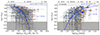 |
Fig. 13. Scaling relations of dark matter, fDM − Σbar and fDM − Vc, shown in the left and right panels, respectively. The blue dashed line represents the best fit to the data in both relations, with the associated intrinsic scatter (ζint) indicated on the plot. We note that the fDM − Vc relation can be seen as the result of a combination of the mass-velocity and mass-size relations. The color codes used for data in both panels are consistent with Figure 11. We note that the uncertainties on data points represent the 68% confidence interval. |


These relations were fit by minimizing the intrinsic scatter. As shown in Figure 13, the dark matter fraction displays a negative correlation with baryon surface density, which is expected and observed at lower redshifts (see McGaugh 2010). On the contrary, it exhibits a positive correlation with circular velocity. Together these relations imply that, although the dynamics of galaxies are dominated by dark matter, the baryons still play an important role in hampering the presence of dark matter, i.e., the evolutionary stages of baryonic matter most likely seem to strongly impact the distribution of dark matter within galaxies. This has long been known at low redshift, but it is highly interesting that the trend seems to continue at higher redshift, too.
To thoroughly examine the scenario postulated above, we divided our full sample into two stellar mass bins: a low-mass bin (Mstar ≤ 1010 M⊙) and a high-mass bin (Mstar > 1010 M⊙). We plotted the Σbar(< Rout)−fDM(< Rout) correlations in the first panel of Figure 14. We note to the reader that this relation is plotted exclusively for objects with fDM > 0. The low stellar mass objects are represented by bright yellow, while the high mass objects are depicted in orange. We observed that the Σbar(< Rout)−fDM(< Rout) relation, as given in Equation (5) remains roughly the same for both mass ranges, indicating no change in the slope. Moreover, this relation remains consistent when observed for fDM(< Ropt), represented by cross marks, i.e., it is valid at different radii within galaxies.
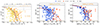 |
Fig. 14. Exploration of the fDM − Σbar relation across different stellar masses and redshift intervals. First panel: fDM − Σbar relation for the low-stellar mass bin (Mstar ≤ 1010 M⊙) in yellow and the high-stellar mass bin (Mstar > 1010 M⊙) in orange. The original best-fit to fDM − Σbar relation is shown blue dashed line, while the best fit of low- and high-stellar mass bins are shown by brown and orange dashed lines, respectively. Second-third panel: fDM − Σbar relation separated for low- and high-stellar masses, left and right panels respectively. In both panels, low-z (z ≤ 1) and high-z (z > 1) galaxies are shown in blue and red, respectively, and corresponding best fits are shown in dark blue and red dashed-lines. In the first panel, median error on the data points is indicated by gray cross. The filled crosses & circles represent the measurements taken within Ropt and Rout, respectively. We note to the reader that these relations are plotted exclusively for objects with fDM > 0, while the full sample is shown in Figure 13. |
Conversely, when we plot VRout − fDM (at both radial scales: Ropt and Rout) for different mass bins we observed a distinct offset in the relation, as shown in the first panel of Figure 15. This suggests that galaxies with high stellar mass are fast-rotating systems with a relatively low dark matter fraction at the outer radius for a given rotational velocity, while the opposite trend is observed for low stellar mass systems. This likely suggests an evolution in the distribution of dark matter due to baryonic processes that take place in massive galaxies.
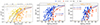 |
Fig. 15. Exploration of the fDM − Vc relation across different stellar masses and redshift intervals. First panel: fDM − Vc relation for the low-stellar mass bin (Mstar ≤ 1010 M⊙) in yellow and the high-stellar mass bin (Mstar > 1010 M⊙) in orange. The best-fit to original fDM − Vc relation is shown blue dashed line given by Equation (6). The Equations corresponds to best fit of low- and high-stellar mass bins is written on the plot, shown by brown and orange dashed lines, respectively. The intrinsic scatter (ζint) associated with fits are printed on plot using same color code. Second-third panel: fDM − Vc relation separated for low- and high-stellar masses, left and right panel respectively. In both panels, low-z (z ≤ 1) and high-z (z > 1) galaxies are shown in blue and red, respectively, and corresponding best-fits are shown by dashed blue and red lines. In all panels, filled crosses and circles represent the measurements taken within Ropt and Rout, respectively, and median error on the data points is indicated by gray crosses. Low surface brightness and low velocity low mass galaxies at high redshift might be missed from the sample. On the other hand, it is clear that DM fractions are lower at fixed rotational velocity at higher redshift, i.e. the plots are not biased on the vertical axis. We note to the reader that these relations are plotted exclusively for objects with fDM > 0 for the clarity on the matter, while the full sample is shown in Figure 13. |
Next, we segregated low and high stellar mass galaxies into low and high redshift (z ≤ 1 and z > 1, respectively) as shown in the second and third panel of Figure 15. We observed very clearly distinct behaviors within the low mass galaxy population. Specifically, at z > 1 in this population, galaxies exhibited lower dark matter fractions at a given rotational velocity compared to the same mass range at z ≤ 1. In contrast, high mass systems demonstrate a more similar behavior for the two redshift bins, with only a slight variation in circular velocities and dark matter fractions14.
We also segregated low and high stellar mass galaxies into low and high redshift (z ≤ 1 and z > 1, respectively) for the baryon surface density relation, as shown in the second and third panel of Figure 14. We notice that in the high stellar mass bin, both low and high-z galaxies follows a similar trend with the same shape as given by Equation (5). The same is true for the low-z galaxies of the low stellar mass bin. However, we noted that the high-z galaxies of the low stellar mass bin display a sharp cutoff at surface densities lower than log(Σbar(< Rout)) ≈ 8.0. This is most likely hinting to an observational bias, i.e., low baryon density galaxies seem to be missing at z > 1. This causes the fit to not follow the Equation 5, but the discrepancy is not as clear visually as for the VRout − fDM(< Rout) relation where the redshift evolution is obvious.
5. Caveats
We estimated the dark matter fraction using a halo-model independent approach, assuming an exponential thin disk distribution for stars and gas. Our analysis provides reliable measurements of the dark matter fraction within different radii: Re, Ropt, and Rout. However, it is important to note that only 20% (53 objects) of the total sample (263 objects) satisfy the criterion Re > PSF. Nevertheless, we report that galaxies are not dark matter deficient at high-z, especially, within 1 − 3Re. Although we report a high dark matter fraction within Re for the high-z galaxies in a larger sample, we advise the reader to interpret these measurements with caution. For instance, the JWST photometry will have the capability to resolve the inner stellar disk and bulge components of galaxies (see also Section E and Figure E.2). Moreover, deep spectroscopic observations will further improve the shape of the rotation curves, as reported in Puglisi et al. (2023, their Fig. 2). Both the former and the latter will impose even tighter constraints on the dark matter distribution in the inner regions of galaxies, which may differ from the results presented here. In particular, the geometry of the disk, especially the gaseous disk, could be different (Romeo et al. 2020; Renaud et al. 2021; Romeo et al. 2023), whilst many systematic uncertainties in the actual stellar mass and gas mass could change the results, although we have shown in Section 4 that it would take a very serious mismatch to erase the dark matter signature from the rotation curves entirely.
Our analysis yields unphysical dark matter fractions for ∼22% of the sample due to Mdyn < Mbar, and an additional ∼15% exhibits low dark matter fraction (0-0.2) within Ropt and Rout, see Figures 11 and E.1. In order to understand these objects, we carefully examined their rotation curves, moment maps, and high-resolution images, yet no apparent anomalies were found. Consequently, our guess is that the photometric stellar masses of these galaxies are likely overestimated. The reason is, SED fitting involves modeling of observed SED by comparing it to a grid of model spectra. The accuracy of the derived stellar mass depends on the assumptions made in these models, such as the choice of star formation histories, stellar population synthesis models, initial mass function (IMF), dust attenuation laws etc. If these assumptions do not accurately represent the true physical conditions of the galaxy (e.g., fraction of binary stars), it can introduce systematic errors (see, e.g., Pacifici et al. 2023; Leja et al. 2019), which may impact the dark matter estimates and its trend as a function of stellar mass or redshift, for example. Moreover, uncertainties in the gas scaling relations (reported in Section 2.4) could also impact the total baryonic mass and consequently the dark matter estimates.
To comprehensively assess the impact of overall uncertainty in stellar mass, star-formation rate, and gas scaling relations, we estimated the dark matter fraction under two scenarios: one accounting for statistical and systematic uncertainties (referred to as Case-1) and with only statistical uncertainties (referred to as Case-2). We conducted Monte Carlo sampling with 10 000 realizations to propagate errors on all parameters. In Case-1, statistical and systematic uncertainties on stellar masses are 0.04 and 0.14 dex, respectively, while for star formation rates, they are 0.04 and 0.25 dex, respectively (cf. Pacifici et al. 2023). During the computation of molecular and atomic gas masses, as defined in Section 2.4, we incorporated an additional uncertainty of 0.3 dex (error in gas scaling relations) for each component individually (H2 and HI masses). Conversely, in Case-2, only statistical uncertainties on stellar mass and star-formation rates were considered for the analysis. Upon comparison, we observed only an increase of 1% in the dark matter in Case-2 than Case-1. In both cases, the overall trends of the dark matter fraction as a function of stellar mass, galactic scales, and redshift remained consistent, albeit the large errors in case-1. In this work we present the results of Case-1, i.e., modeling statistical as well systematic uncertainties.
Furthermore, the issues regarding Mdyn < Mstar have been previously reported in studies concerning high-z galaxies, including works by Wisnioski et al. (2015), Förster Schreiber & Wuyts (2020), and Sharma et al. (2021a). We propose several conditions under which the dynamical mass could appear smaller than the baryonic mass:
-
Incomplete sampling of the velocity distribution: If the velocity measurements used to estimate the dynamical mass are limited to only a small fraction of the stars or gas in a galaxy, the resulting estimate of the dynamical mass could be lower than the actual value, as hinted in Puglisi et al. (2023). In this analysis, we extracted the best possible kinematics information available in our datasets, but with better dataset these estimates will improve further.
-
Non-equilibrium conditions: If a galaxy has recently undergone a major disturbance, such as a merger or a violent epoch of star formation, the velocity distribution of its stars and gas may not yet have settled into a stable equilibrium (Riechers et al. 2014; Lemaux 2017; Förster Schreiber & Wuyts 2020, and reference therein). In this case, the dynamical masses based on rotation velocity could be lower than the actual value. In our sample, we visually inspect the galaxy rotation curves moment maps, and high resolution photometry, and discard all the potential mergers. However, it is worth noting that our understanding of the merging history of galaxies at high-z is still limited.
-
Non-circular orbits: If the stars and gas in a galaxy are on non-circular orbits, the velocity measurements used to estimate the dynamical mass will only provide a lower limit on the actual mass (Binney & Tremaine 1987, references therein). This can only be understood with future high-resolution spectroscopy. That is, there is room for improvement in our dynamical masses.
On the contrary, the most massive galaxies in our sample with log(Mstar [M⊙]) > 10.7 exhibit a significant amount of dark matter across the galactic scales, surpassing the average dark matter fraction observed in the overall sample. Remarkably, the dark matter halos of these galaxies are more massive than those observed in massive systems in the local Universe, such as the Milky Way and Andromeda (see Figure 10 and Figure 11), the two plausible scenarios are:
-
These massive galaxies may have followed distinct evolutionary pathways, resulting in the formation of exceptionally massive dark matter halos. Or,
-
The baryonic masses of these objects are underestimated, for instance due to the presence of massive compact objects. Indeed, if a galaxy contains a substantial number of compact objects, such as black holes or neutron stars, their gravitational influence could dominate the motion of stars and gas, leading to an overestimate of the dynamical mass (Naab & Ostriker 2017, see references therein)
Finally, it is important to highlight that galaxies with low baryon surface densities (log(Σbar(< Rout)) < 8.0), often categorized as low surface-brightness galaxies, are noticeably absent from our sample at z > 1, as depicted in Figure 14 (second panel). This absence is potentially attributable to Tolman Dimming, a relativistic phenomenon in which the observed surface brightness of a celestial object diminishes as (1 + z)2 (Tolman 1930; Pahre et al. 1996; Sandage 2010). Consequently, low surface-brightness galaxies could go missing in high-redshift observations. It should also be noted that these galaxies present challenges for observation even in the local Universe. To acquire resolved rotation curves for such systems, observatories with substantial aperture sizes, such as the forthcoming Extremely Large Telescope, would be required.
With these caveats in mind, it is noteworthy that the majority (∼70%) of galaxies in our sample contain significant amount of dark matter, consistent with the findings of a previous study conducted by Sharma et al. (2021b), and not very different from local galaxies. Consequently, the reliability of our sample, techniques, and measurements instills confidence and provides a firm foundation for further discussion on: (1) the evolution of dark matter in galaxies across cosmic time, and (2) challenges in constraining the dark matter at high-z.
6. Discussion
In this section, we discuss the main findings of this work.
6.1. Dark matter fraction:
In local star-forming galaxies, where dark matter is believed to constitute the majority of the mass in most galaxies, dark matter fraction (within Ropt) estimates typically range from 70% to 90% of the total mass. The dark matter fraction in these galaxies is relatively higher in the outskirts compared to the inner regions, indicating that the inner regions are dominated by baryonic processes while the dynamics of the outskirts is governed by dark matter (Rubin et al. 1980; Persic et al. 1996; Martinsson et al. 2013; Courteau & Dutton 2015; McGaugh 2016). A similar trend is observed in high-z galaxies, as shown in Figures 11 & 12. Based on the datasets presented in this study, we show that the galaxies at high redshifts (0.75 < z < 1.8) are predominantly influenced by dark matter from Ropt to Rout, with fractions ranging from 50% to 90%.
While we identify dark matter-dominated systems at high-z, we observe a significant scatter in relations, such as fDM − Mstar, fDM − z, fDM − VRout, and Σbar − fDM, see Figures 11, 12, & 13, respectively. A similar scatter is also reported in Sharma et al. (2021b). The scatters in these relations suggest that these galaxies might still be undergoing the process of building or acclimating their distribution of baryons and dark matter. In other words, they are at different stages of ‘galaxy assembly’15. The scatter in the dark matter fraction itself may stem from various other factors, including differences in formation history of galaxies, the irregular distribution of baryons that can affect the distribution of dark matter, and the environment in which these galaxies reside (Dutton et al. 2016; Behroozi et al. 2019). Moreover, it could also be due to the diversity in the dark matter halo properties, which are closely coupled to the properties of the baryonic matter. However, we note that if any systematic uncertainties in estimating baryonic masses have been neglected, this would naturally increase the scatter, never decrease it.
6.2. Dark matter halo assembly:
According to the current cosmological model, Lambda Cold Dark Matter (ΛCDM), dark matter plays a fundamental role in the assembly of cosmic structures in the Universe. This assembly process follows a hierarchical pattern, wherein smaller structures form first and subsequently merge to form larger ones, and gradually increase in mass and size (Peebles 1993). This hierarchical merging process is primarily driven by gravity and influenced by the distribution of matter in the Universe, encompassing both dark and baryonic matter. Since dark matter is invisible and cannot be directly observed, studying the distribution and properties of baryons, such as surface density and motion governed by the total gravitational potential, provides a way to gain insights into the distribution of dark matter and its assembly history.
In accordance with the aforementioned concepts, we investigated Σbar − fDM relation, which was previously examined by Genzel et al. (2020) within the effective radius. Expanding upon their work, we extended this relation to encompass the outer radius (Ropt and Rout). Notably, our data well fit the relationship described by Equation (5), with an intrinsic scatter of 0.25 dex. Intriguingly, we observed that the Σbar − fDM relation maintains a consistent slope also when examined at the optical radius, and the outer radius in both low and high mass systems, as illustrated in the first panel of Figure 14. Moreover, this relationship remains unchanged across different redshift ranges, as demonstrated in second-third panel of Figure 14. Thus, the Σbar − fDM relation exhibits a uniform nature, implying that the influence of baryonic matter on dark matter appears to be similar across various stellar mass ranges, and redshift intervals. However, uncertainty on the individual measurement and intrinsic scatter in this relation is very high. Only high-quality data will allow the exact scatter of this relation to be pinpointed. Taking the current scatter at face value would indeed indicate that the relation is not fundamental (Milgrom 1983; Famaey & McGaugh 2012) but that galaxies are likely at distinct evolutionary stages, such as being in the process of establishing their respective disks.
On the other hand, when analyzing the relationship between Vc − fDM(< Rout), as depicted in the right panel of Figure 13, the correlation was slightly tighter, with an intrinsic scatter of 0.23 dex. However, this relation, which is the result of a combination of the mass-velocity and mass-size relations is not at all universal, as further exploration of this relationship for low and high stellar mass galaxies, as illustrated in the first panel of Figure 15, revealed the emergence of distinct sequences as a function of both mass and redshift. Galaxies with high stellar mass naturally exhibit a lower fraction of dark matter at fixed rotational velocity, which is related to their baryonic size and dark matter halos being different from lower stellar mass ones. In the second-third panel of Figure 15, we divide the fDM − Vc relation of low and high stellar masses in low and high-z (z ≤ 1 and z > 1, respectively). Notably, a distinct offset was observed between low-z and high-z objects of the low-mass bin (log(Mstar [M⊙]) ≤ 1010). Specifically, low-mass galaxies at high-z exhibit a lower fraction of dark matter at fixed rotational velocity. This is intriguing, suggesting that low-mass mass galaxies most likely undergo higher degree of evolution in terms of their respective dark matter and baryon distribution. On the other hand, high-mass systems already seems to be settled at higher-z, as evidenced in the third panel of Figure 15.
6.3. Uncertainties & limitations:
As highlighted in caveats, in Section 5, the study of dark matter fraction at high-z is very challenging and requires significant refinements in both baryonic constraints and kinematic modeling. In this section, we discuss a few key challenges of the field.
For baryons, SED fitting techniques, which are commonly used to estimate stellar masses and SFRs, exhibit substantial offsets from each other (Leja et al. 2019; Pacifici et al. 2023). These discrepancies not only lead to larger uncertainties in stellar masses and SFRs, but also impact the gas mass scaling relations. For instance, Tacconi et al. (2018), molecular gas mass scaling relation, uses the Speagle et al. (2014) main-sequence relation (M*-SFR plane). At z ∼ 0.1, the Speagle et al. (2014) main sequence differs from Chang et al. (2015) by ∼ 0.4 dex, and at z ∼ 1, it is ∼ 0.25 dex off from the 3DHST study (Nelson et al. 2021). At higher redshifts, this offset is not yet quantified. Therefore, the systematic offset and observed scatter in gas scaling relation, which relay on main-sequence relation is complex to accurately quantify, and beyond of the scope of this study.
Due to the lack of direct measurements of HI gas at high redshifts (z > 1), accurate gas masses at z > 1 are still unavailable. At z < 1, HI mass scaling relations are derived using stacking analyses, as current observing facilities only allow HI signal detection without resolution Chowdhury et al. (2022). These HI scaling relations are general and not specifically for star-forming disk-like galaxies. That is, we can use them as a first order approximation, but they are not accurate. Refining HI mass relations will requires future observations from the Square Kilometer Array.
Moreover, current kinematic modeling techniques have limitations, such as not accounting for non-circular motions, gas inflows, and outflows Oman et al. (2019). Consequently, accurately modeling the total dynamical mass of the system is challenging. This issue can only be resolved with very high-resolution large galactic-scale surveys at high redshifts, which are currently not feasible even in optical and near-infrared astronomy. Further progress might only be possible with the construction of Extremely Large Telescope.
Lastly, the ‘Tolman Dimming’ effect, hinders the observation of low to intermediate mass galaxies at higher redshifts. Consequently, our observations at high-z are biased toward more massive systems. Additionally, we know that, in the local Universe and at high-z, dark matter shows a slightly decreasing trend as a function of stellar mass, i.e., massive galaxies show relatively low dark matter fraction. Therefore, the observed low dark matter fraction at high-z, or the decreasing trend of dark matter fraction as a function of redshift, could be an artifact caused by the absence of low to intermediate mass galaxies. To accurately constrain the trend of dark matter fraction across cosmic time, further deep observations of low and intermediate mass galaxies at high redshifts are required.
Nevertheless, given the best possible information available on baryonic content, observed kinematics, and their uncertainties, we present conservative dark matter fraction estimates to the best of our abilities. However, we acknowledge that these findings require further refinement, which will be achieved as the field progresses.
7. Summary and conclusions
Through this study, our aim was to investigate the fraction of dark matter across different galactic scales and cosmic time. To achieve this objective, we utilized a substantial sample consisting of 263 main-sequence star-forming disk-like galaxies within the redshift range 0.6 ≤ z ≤ 2.2. This sample encompasses 73 galaxies from the KMOS3D survey, 21 from the KGES survey, and 169 from the KROSS survey. We performed 3D forward modeling of datacubes using the 3DBarolo code, as described in Section 3. Figure 5 provides an illustrative example of the kinematic modeling results obtained using 3DBarolo, displaying the velocity distribution (moment-1 and moment-2 maps), data, model, and residuals, followed by the major axis PV diagram and the velocity dispersion curve. We applied pressure support corrections to the rotation curves inferred from 3DBarolo, these pressure corrected rotation curves are referred to as intrinsic rotation curves.
To estimate the dark matter fraction, we subtracted the baryon contribution from the intrinsic rotation curves, assuming that both the star and gas are rotationally supported and confined to an exponential disk. The residual contribution was assumed to originate from the dark matter, which was required to explain the observed kinematics. For a detailed explanation of this methodology, we refer the reader to Sections C and D. We estimated the dark matter fraction within Re till Rout (see Sects. 4.1 & 4.2 and Figures 10 & 11). Additionally, we explored the variation of the dark matter fraction across different redshift ranges, presented in Section 4.3 and illustrated in Figure 12. Furthermore, we investigated the interplay between baryonic matter and dark matter by examining the scaling relations of dark matter with baryon surface density and circular velocity at the outer radius of galaxies in Section 4.4, as shown in Figures 13, 14, and 15. The results obtained from these analyses offer valuable insights into the role of dark matter in shaping galaxies. Our key findings are as follows:
-
Similar to local disk galaxies, high-z galaxies also exhibit dark matter-dominated outer halos (from Re to Rout), with a dark matter fraction (fDM) ranging between 50% and 90%. It is noteworthy that at z = 1 − 1.8, the median value of fDM remains above 50% across all the galactic scales, which is very similar to local disk galaxies.
-
Due to the lack of resolved observations within
 , it remains uncertain whether or not the dark matter fraction in high-z disk-like galaxies gradually increases from
  to Rout. To establish a clear trend of dark matter fraction as a function of redshift, deeper observations of low- and intermediate-mass galaxies at high redshift are required along with precise measurements of their baryonic and total dynamical masses.
 -
The Vc − fDM relation revealed distinct sequences with stellar mass and redshift intervals. Specifically, low stellar mass (Mstar ≤ 1010 M⊙) galaxies exhibit a higher degree of dynamical evolution with clearly lower dark matter fractions at a given rotational velocity at higher redshift (z > 1). This can potentially be attributed to the hierarchical assembly of dark matter halos governing the evolution of galaxies.
-
The Σbar − fDM relation demonstrates a consistent trend, slope, and scatter across different stellar mass ranges and redshift intervals, indicating a universal nature of the influence of baryonic matter on the distribution of dark matter. The relation also holds at different radii within galaxies. This implies that the interplay between baryons and dark matter in galaxies is the same, regardless of their mass, size, and age.
-
Numerous uncertainties related to the baryonic content result in substantial errors in the estimated dark matter fraction of galaxies. By reducing these errors, through a combination of observational and theoretical improvements, we as a community have the potential to make a significant leap forward in our understanding of galaxy evolution and the properties of dark matter.
Existing studies (including this work) on dark matter in high-redshift galaxies support the presence of dark matter but fall short on being able to robustly establish further insights, such as its radial distribution. Nevertheless, these studies represent an important step forward in our understanding of galaxies and dark matter halo evolution. To establish tighter constraints on our findings, the current kinematic modeling techniques need to be amended, as they rely heavily on the assumptions of axisymmetry and dynamical equilibrium, which might not be the case at high-z. More accurate assessment of the baryonic content at high-z is required. Lastly, lower surface-brightness galaxies are underrepresented in high-redshift observations, making high-quality data indispensable for resolving the present conundrums.
Data availability
The catalogs of galaxy physical properties such as stellar mass, gas mass, rotation velocity, dark matter fraction etc. are publicly accessible via Zenodo (https://zenodo.org/records/15458539). Additionally, position–velocity diagrams and velocity dispersion plots for the complete datasets are available at Zenodo (https://zenodo.org/records/15450208). The corresponding datacubes and 3DBarolo model outputs can be provided by the authors upon reasonable request.
In general, the scale length (or radius) is associated with various quantities that decrease exponentially, such as the surface brightness. The disk edge is defined as 3.2 RD ( = 1.89 Re), where the stellar surface luminosity ∝exp(−r/RD). Therefore, scale lengths in terms of the effective radius can be written as: RD = 0.59 Re; Ropt = 1.89 Re; Rout = 2.95 Re.
The line-of-sight velocity is defined as VLOS = Vrot sin θi, where Vrot is the intrinsic rotation and θi is the inclination angle of a galaxy. If a galaxy is face-on (i.e., θi ≈ 0), the intrinsic rotation results are divergent. Additionally, intrinsic rotation in low-inclination (0 < θi ≤ 25) galaxies is often obscured by the superposition of radial and tangential motions, leading to a flattened appearance of the velocity profile. This consideration has been fundamental in RC studies since the beginning (see for instance Persic et al. 1996; Sofue & Rubin 2001). On the other hand, if a galaxy is edge-on, extinction is prominent due to the increased opacity of the galaxy, which dramatically flatten the inner slope of the RCs above 80°, as demonstrated in various works such as Valotto & Giovanelli (2004) and Rhee et al. (2004). This is why, we select the galaxies with inclination angle: 25° ≤θi ≤ 75°.
In IFU-based spectroscopy and imaging, the PSF describes how a point source (like a distant star or galaxies) appears in an observation due to the effects of the imaging system and atmospheric conditions. Similarly, the line spread function describes how a spectral line from a point source is broadened by the spectrograph and other instrumental effects. That is, beam smearing is associated with a poor PSF, while spectral smearing is due to a poor line spread function.
See its documentation, https://bbarolo.readthedocs.io/en/latest/
Nelder-Mead is a gradient free optimization method that finds the minimum of function by iteratively updating the vertices of polytope in n-dimensional space. It is particularly used for optimization problem with non-liner or multi-model objective functions, which is the case of galaxy kinematics.
The following massive galaxies have very high dark matter fractions: COS4_23890 (z = 0.85, M* = 1010.83, fDM = 0.83), U4_19708 (z = 1.66, M* = 1011.26, fDM = 0.64), U4_31577 (z = 1.52, M* = 1011.07, fDM = 0.37), and U4_26875 (z = 1.36, M* = 1011.18, fDM = 0.73), U4_28358 (z = 1.42, M* = 1010.98, fDM = 0.68), U4_21533 (z = 0.92, M* = 1011.11, fDM = 0.46).
Acknowledgments
We thank the anonymous referee for providing valuable comments that have improved the quality of the manuscript. We express our gratitude to Emily Wisnioski and her team, as well as Mark Swinbank and his team, for the public release of KMOS3D and KGES Hα datacubes and catalogs, along with their valuable discussions and support. We also thank Benoit Famaey, Jonathan Freundlich, and Florent Renaud for their efforts in contributing to this paper at various stages. G.S., acknowledges SARAO postdoctoral fellowship (UId No.: 97882), and thanks Ambica Govind for providing HST images of full sample. G.S. also thanks Mihael Petac for various fruitful discussions. GvdV acknowledges funding from the European Research Council (ERC) under the European Union’s Horizon 2020 research and innovation programme under grant agreement No 724857 (Consolidator GrantArcheoDyn). G.S. acknowledge support from the University of Strasbourg Institute for Advanced Study (USIAS), within the French national programme Investment for the Future (Excellence Initiative) IdEx-Unistra. M.M., thanks financial support of the Flemish Fund for Scientific Research (FWO-Vlaanderen), research project G030319N.
References
- Angulo, R. E., & Hahn, O. 2022, Liv. Rev. Comput. Astrophys., 8, 1 [CrossRef] [Google Scholar]
- Behroozi, P., Wechsler, R. H., Hearin, A. P., & Conroy, C. 2019, MNRAS, 488, 3143 [NASA ADS] [CrossRef] [Google Scholar]
- Binney, J., & Tremaine, S. 1987, Galactic dynamics (Princeton, N.J. : Princeton University Press) [Google Scholar]
- Boselli, A., Lequeux, J., & Gavazzi, G. 2002, A&A, 384, 33 [NASA ADS] [CrossRef] [EDP Sciences] [Google Scholar]
- Bosma, A. 1981, AJ, 86, 1791 [NASA ADS] [CrossRef] [Google Scholar]
- Bouché, N. F., Bera, S., Krajnović, D., et al. 2022, A&A, 658, A76 [NASA ADS] [CrossRef] [EDP Sciences] [Google Scholar]
- Brammer, G. B., van Dokkum, P. G., Franx, M., et al. 2012, ApJS, 200, 13 [Google Scholar]
- Bruzual, G., & Charlot, S. 2003, MNRAS, 344, 1000 [NASA ADS] [CrossRef] [Google Scholar]
- Bullock, J. S., & Boylan-Kolchin, M. 2017, ARA&A, 55, 343 [Google Scholar]
- Burkert, A. 1995, ApJ, 447, L25 [NASA ADS] [Google Scholar]
- Burkert, A., Genzel, R., Bouché, N., et al. 2010, ApJ, 725, 2324 [Google Scholar]
- Burkert, A., Schreiber, N. F., Genzel, R., et al. 2016, ApJ, 826, 214 [CrossRef] [Google Scholar]
- Calzetti, D., Kinney, A. L., & Storchi-Bergmann, T. 1994, ApJ, 429, 582 [Google Scholar]
- Calzetti, D., Armus, L., Bohlin, R. C., et al. 2000, ApJ, 533, 682 [NASA ADS] [CrossRef] [Google Scholar]
- Cappellari, M., Scott, N., Alatalo, K., et al. 2013, MNRAS, 432, 1709 [Google Scholar]
- Casey, C. M., Kartaltepe, J. S., Drakos, N. E., et al. 2023, ApJ, 954, 31 [NASA ADS] [CrossRef] [Google Scholar]
- Chabrier, G. 2003, PASP, 115, 763 [Google Scholar]
- Chang, Y.-Y., van der Wel, A., da Cunha, E., & Rix, H.-W. 2015, ApJS, 219, 8 [Google Scholar]
- Charlot, S., & Fall, S. M. 2000, ApJ, 539, 718 [Google Scholar]
- Chowdhury, A., Kanekar, N., & Chengalur, J. N. 2022, ApJ, 941, L6 [NASA ADS] [CrossRef] [Google Scholar]
- Cormier, D., Bigiel, F., Wang, J., et al. 2016, MNRAS, 463, 1724 [NASA ADS] [CrossRef] [Google Scholar]
- Courteau, S., & Dutton, A. A. 2015, ApJ, 801, L20 [Google Scholar]
- da Cunha, E., Charlot, S., & Elbaz, D. 2008, MNRAS, 388, 1595 [Google Scholar]
- Daddi, E., Elbaz, D., Walter, F., et al. 2010, ApJ, 714, L118 [NASA ADS] [CrossRef] [Google Scholar]
- Dekel, A., Freundlich, J., Jiang, F., et al. 2021, MNRAS, 508, 999 [NASA ADS] [CrossRef] [Google Scholar]
- Di Teodoro, E., Fraternali, F., & Miller, S. 2016, A&A, 594, A77 [NASA ADS] [CrossRef] [EDP Sciences] [Google Scholar]
- Drew, P. M., Casey, C. M., Burnham, A. D., et al. 2018, ApJ, 869, 58 [NASA ADS] [CrossRef] [Google Scholar]
- Dutton, A. A., Macciò, A. V., Dekel, A., et al. 2016, MNRAS, 461, 2658 [NASA ADS] [CrossRef] [Google Scholar]
- El-Zant, A. A., Freundlich, J., & Combes, F. 2016, MNRAS, 461, 1745 [Google Scholar]
- Famaey, B., & McGaugh, S. S. 2012, Liv. Rev. Relativ., 15, 10 [Google Scholar]
- Förster Schreiber, N. M., & Wuyts, S. 2020, ARA&A, 58, 661 [Google Scholar]
- Förster Schreiber, N. M., Genzel, R., Lehnert, M. D., et al. 2006, ApJ, 645, 1062 [Google Scholar]
- Freeman, K. 1970, ApJ, 160, 811 [NASA ADS] [CrossRef] [Google Scholar]
- Freundlich, J., Combes, F., Tacconi, L. J., et al. 2019, A&A, 622, A105 [NASA ADS] [CrossRef] [EDP Sciences] [Google Scholar]
- Freundlich, J., Dekel, A., Jiang, F., et al. 2020, MNRAS, 491, 4523 [NASA ADS] [CrossRef] [Google Scholar]
- Fu, J., Guo, Q., Kauffmann, G., & Krumholz, M. R. 2010, MNRAS, 409, 515 [Google Scholar]
- Genzel, R., Tacconi, L. J., Lutz, D., et al. 2015, ApJ, 800, 20 [Google Scholar]
- Genzel, R., Schreiber, N. F., Ubler, H., et al. 2017, Nature, 543, 397 [NASA ADS] [CrossRef] [Google Scholar]
- Genzel, R., Price, S. H., Übler, H., et al. 2020, ApJ, 902, 98 [NASA ADS] [CrossRef] [Google Scholar]
- Giacconi, R., Rosati, P., Tozzi, P., et al. 2001, ApJ, 551, 624 [Google Scholar]
- Gillman, S., Tiley, A. L., Swinbank, A. M., et al. 2020, MNRAS, 492, 1492 [Google Scholar]
- Harris, W. E., Remus, R.-S., Harris, G. L. H., & Babyk, I. V. 2020, ApJ, 905, 28 [CrossRef] [Google Scholar]
- Harrison, C., Johnson, H., Swinbank, A., et al. 2017, MNRAS, 467, 1965 [NASA ADS] [CrossRef] [Google Scholar]
- Häußler, B., Bamford, S. P., Vika, M., et al. 2013, MNRAS, 430, 330 [Google Scholar]
- Johnson, H. L., Harrison, C. M., Swinbank, A. M., et al. 2018, MNRAS, 474, 5076 [NASA ADS] [CrossRef] [Google Scholar]
- Karukes, E., & Salucci, P. 2017, MNRAS, 465, 4703 [NASA ADS] [CrossRef] [Google Scholar]
- Kassin, S. A., de Jong, R. S., & Weiner, B. J. 2006, ApJ, 643, 804 [Google Scholar]
- Keres, D., Yun, M. S., & Young, J. S. 2003, ApJ, 582, 659 [NASA ADS] [CrossRef] [Google Scholar]
- Kriek, M., van Dokkum, P. G., Labbé, I., et al. 2009, ApJ, 700, 221 [Google Scholar]
- Lagos, C. D. P., Baugh, C. M., Lacey, C. G., et al. 2011, MNRAS, 418, 1649 [CrossRef] [Google Scholar]
- Lang, P., Schreiber, N. M. F., Genzel, R., et al. 2017, ApJ, 840, 92 [NASA ADS] [CrossRef] [Google Scholar]
- Lawrence, A., Warren, S., Almaini, O., et al. 2007, MNRAS, 379, 1599 [NASA ADS] [CrossRef] [Google Scholar]
- Lehmer, B. D., Brandt, W., Alexander, D., et al. 2005, ApJS, 161, 21 [NASA ADS] [CrossRef] [Google Scholar]
- Leja, J., Johnson, B. D., Conroy, C., et al. 2019, ApJ, 877, 140 [NASA ADS] [CrossRef] [Google Scholar]
- Lelli, F., Zhang, Z.-Y., Bisbas, T. G., et al. 2023, A&A, 672, A106 [NASA ADS] [CrossRef] [EDP Sciences] [Google Scholar]
- Lemaux, B. C. 2017, Early stages of Galaxy Cluster Formation, 43 [Google Scholar]
- Leroy, A. K., Walter, F., Brinks, E., et al. 2008, AJ, 136, 2782 [Google Scholar]
- Li, Z., Dekel, A., Mandelker, N., Freundlich, J., & François, T. L. 2023, MNRAS, 518, 5356 [Google Scholar]
- Martin, A. M., Papastergis, E., Giovanelli, R., et al. 2010, ApJ, 723, 1359 [NASA ADS] [CrossRef] [Google Scholar]
- Martinsson, T. P. K., Verheijen, M. A. W., Westfall, K. B., et al. 2013, A&A, 557, A131 [NASA ADS] [CrossRef] [EDP Sciences] [Google Scholar]
- Martorano, M., van der Wel, A., Bell, E. F., et al. 2023, ApJ, 957, 46 [NASA ADS] [CrossRef] [Google Scholar]
- McGaugh, S. 2010, Am. Inst. Phys. Conf. Ser., 1240, 13 [Google Scholar]
- McGaugh, S. S. 2016, ApJ, 816, 42 [Google Scholar]
- Milgrom, M. 1983, ApJ, 270, 365 [Google Scholar]
- Momcheva, I. G., Brammer, G. B., van Dokkum, P. G., et al. 2016, ApJS, 225, 27 [Google Scholar]
- Naab, T., & Ostriker, J. P. 2017, ARA&A, 55, 59 [Google Scholar]
- Navarro, J. F., Frenk, C. S., & White, S. D. M. 1996, ApJ, 462, 563 [Google Scholar]
- Nelson, E. J., Tacchella, S., Diemer, B., et al. 2021, MNRAS, 508, 219 [NASA ADS] [CrossRef] [Google Scholar]
- Nestor Shachar, A., Price, S. H., Förster Schreiber, N. M., et al. 2023, ApJ, 944, 78 [NASA ADS] [CrossRef] [Google Scholar]
- Noeske, K. G., Weiner, B. J., Faber, S. M., et al. 2007, ApJ, 660, L43 [CrossRef] [Google Scholar]
- Oman, K. A., Marasco, A., Navarro, J. F., et al. 2019, MNRAS, 482, 821 [NASA ADS] [CrossRef] [Google Scholar]
- Pacifici, C., Iyer, K. G., Mobasher, B., et al. 2023, ApJ, 944, 141 [NASA ADS] [CrossRef] [Google Scholar]
- Pahre, M. A., Djorgovski, S. G., & de Carvalho, R. R. 1996, ApJ, 456, L79 [NASA ADS] [CrossRef] [Google Scholar]
- Peebles, P. J. E. 1993, Principles of Physical Cosmology (Princeton: Princeton University Press) [Google Scholar]
- Peng, C. Y., Ho, L. C., Impey, C. D., & Rix, H.-W. 2010, AJ, 139, 2097 [Google Scholar]
- Persic, M., & Salucci, P. 1990, MNRAS, 247, 349 [NASA ADS] [Google Scholar]
- Persic, M., Salucci, P., & Stel, F. 1996, MNRAS, 281, 27 [Google Scholar]
- Petač, M. 2020, Phys. Rev. D, 102, 123028 [Google Scholar]
- Pontzen, A., & Governato, F. 2012, MNRAS, 421, 3464 [NASA ADS] [CrossRef] [Google Scholar]
- Pontzen, A., & Governato, F. 2014, Nature, 506, 171 [NASA ADS] [CrossRef] [Google Scholar]
- Price, S. H., Kriek, M., Shapley, A. E., et al. 2016, ApJ, 819, 80 [Google Scholar]
- Price, S. H., Shimizu, T. T., Genzel, R., et al. 2021, ApJ, 922, 143 [NASA ADS] [CrossRef] [Google Scholar]
- Puglisi, A., Dudzevičiūtė, U., Swinbank, M., et al. 2023, MNRAS, 524, 2814 [NASA ADS] [CrossRef] [Google Scholar]
- Renaud, F., Romeo, A. B., & Agertz, O. 2021, MNRAS, 508, 352 [NASA ADS] [CrossRef] [Google Scholar]
- Rhee, G., Valenzuela, O., Klypin, A., Holtzman, J., & Moorthy, B. 2004, ApJ, 617, 1059 [Google Scholar]
- Riechers, D. A., Carilli, C. L., Capak, P. L., et al. 2014, ApJ, 796, 84 [Google Scholar]
- Rodighiero, G., Daddi, E., Baronchelli, I., et al. 2011, ApJ, 739, L40 [Google Scholar]
- Romeo, A. B., Agertz, O., & Renaud, F. 2020, MNRAS, 499, 5656 [NASA ADS] [CrossRef] [Google Scholar]
- Romeo, A. B., Agertz, O., & Renaud, F. 2023, MNRAS, 518, 1002 [Google Scholar]
- Rubin, V. C., Ford, W. K., Jr, & Thonnard, N. 1980, ApJ, 238, 471 [NASA ADS] [CrossRef] [Google Scholar]
- Sales, L. V., Wetzel, A., & Fattahi, A. 2022, Nat. Astron., 6, 897 [NASA ADS] [CrossRef] [Google Scholar]
- Salucci, P. 2019, A&ARv, 27, 2 [NASA ADS] [CrossRef] [Google Scholar]
- Sandage, A. 2010, AJ, 139, 728 [Google Scholar]
- Scoville, N., Abraham, R. G., Aussel, H., et al. 2007, ApJS, 172, 38 [NASA ADS] [CrossRef] [Google Scholar]
- Sérsic, J. L. 1963, Bol. Asoc. Argentina Astron. La Plata Argentina, 6, 41 [Google Scholar]
- Sharma, G., Salucci, P., Harrison, C. M., van de Ven, G., & Lapi, A. 2021a, MNRAS, 503, 1753 [CrossRef] [Google Scholar]
- Sharma, G., Salucci, P., & van de Ven, G. 2021b, A&A, 653, A20 [NASA ADS] [CrossRef] [EDP Sciences] [Google Scholar]
- Sharma, G., Salucci, P., & van de Ven, G. 2022, A&A, 659, A40 [NASA ADS] [CrossRef] [EDP Sciences] [Google Scholar]
- Sharples, R. 2014, Proc. Int. Astron. Union, 10, 11 [NASA ADS] [CrossRef] [Google Scholar]
- Skelton, R. E., Whitaker, K. E., Momcheva, I. G., et al. 2014, ApJS, 214, 24 [Google Scholar]
- Sobral, D., Matthee, J., Best, P. N., et al. 2015, MNRAS, 451, 2303 [Google Scholar]
- Sofue, Y., & Rubin, V. 2001, ARA&A, 39, 137 [NASA ADS] [CrossRef] [Google Scholar]
- Speagle, J. S., Steinhardt, C. L., Capak, P. L., & Silverman, J. D. 2014, ApJS, 214, 15 [Google Scholar]
- Steidel, C. C., Adelberger, K. L., Dickinson, M., et al. 1998, ApJ, 492, 428 [Google Scholar]
- Stott, J. P., Swinbank, A., Johnson, H. L., et al. 2016, MNRAS, 457, 1888 [Google Scholar]
- Tacconi, L. J., Genzel, R., Saintonge, A., et al. 2018, ApJ, 853, 179 [Google Scholar]
- Tamm, A., Tempel, E., Tenjes, P., Tihhonova, O., & Tuvikene, T. 2012, A&A, 546, A4 [NASA ADS] [CrossRef] [EDP Sciences] [Google Scholar]
- Teodoro, E. D., & Fraternali, F. 2015, MNRAS, 451, 3021 [NASA ADS] [CrossRef] [Google Scholar]
- Tiley, A. L., Swinbank, A., Harrison, C., et al. 2019a, MNRAS, 485, 934 [NASA ADS] [CrossRef] [Google Scholar]
- Tiley, A., Bureau, M., Cortese, L., et al. 2019b, MNRAS, 482, 2166 [NASA ADS] [CrossRef] [Google Scholar]
- Tiley, A. L., Gillman, S., Cortese, L., et al. 2021, MNRAS, 506, 323 [Google Scholar]
- Tolman, R. C. 1930, Proc. Nat. Academy Sci., 16, 511 [Google Scholar]
- Tully, R. B., & Fisher, J. R. 1977, A&A, 54, 661 [NASA ADS] [Google Scholar]
- Übler, H., Genzel, R., Tacconi, L. J., et al. 2018, ApJ, 854, L24 [CrossRef] [Google Scholar]
- Übler, H., Genzel, R., Wisnioski, E., et al. 2019, ApJ, 880, 48 [Google Scholar]
- Valentino, F., Brammer, G., Gould, K. M. L., et al. 2023, ApJ, 947, 20 [NASA ADS] [CrossRef] [Google Scholar]
- Valotto, C., & Giovanelli, R. 2004, AJ, 128, 115 [Google Scholar]
- van Albada, T. S., Bahcall, J. N., Begeman, K., & Sancisi, R. 1985, ApJ, 295, 305 [Google Scholar]
- van Dokkum, P. G., & Brammer, G. 2010, ApJ, 718, L73 [NASA ADS] [CrossRef] [Google Scholar]
- Weijmans, A.-M., de Zeeuw, P. T., Emsellem, E., et al. 2014, MNRAS, 444, 3340 [Google Scholar]
- Whitaker, K. E., van Dokkum, P. G., Brammer, G., & Franx, M. 2012, ApJ, 754, L29 [Google Scholar]
- Wisnioski, E., Förster Schreiber, N. M., Wuyts, S., et al. 2015, ApJ, 799, 209 [Google Scholar]
- Wisnioski, E., Förster Schreiber, N. M., Fossati, M., et al. 2019, ApJ, 886, 124 [Google Scholar]
- Wuyts, S., Förster Schreiber, N. M., van der Wel, A., et al. 2011, ApJ, 742, 96 [NASA ADS] [CrossRef] [Google Scholar]
- Wuyts, S., Förster Schreiber, N. M., Wisnioski, E., et al. 2016, ApJ, 831, 149 [Google Scholar]
- Zwaan, M. A., Meyer, M. J., Staveley-Smith, L., & Webster, R. L. 2005, MNRAS, 359, L30 [NASA ADS] [CrossRef] [Google Scholar]
Appendix A: Signal to noise estimation
Observations of high-z galaxies are often characterized by limited spatial resolution and low S/Ns, posing challenges for kinematic modeling. Therefore, before performing kinematic modeling with 3DBarolo, we first examine the integrated spectra of the Hα datacubes.16
Prior to any analysis, we crop the publicly available datacubes into smaller sub-cubes centered on Hα. Each cropped Hα sub-cube consists of 31 spectral channels, spanning 15 channels on either side of the central Hα wavelength (λHα), while no cropping is applied in the spatial dimensions. These sub-cubes are utilized to compute the integrated spectra, 1D spectra (defined below), and Hα images.
Furthermore, the publicly available Hα datacubes include both flux and noise extensions, enabling us to estimate the S/N(λ) = Fsignal(λ)/Fnoise(λ), as illustrated in the upper panel of Figure A.1. Additionally, we evaluate the integrated Hα images of each galaxy.17
In our analysis, the S/N provides a quantitative measure of the data quality (shown in the first and second columns of Figure A.2), while qualitative assessments are based on the visual inspection of Hα images (shown in the third column of Figure A.2). Based on this combined quantitative and qualitative inspection, we classify the sample into three categories:
-
Q1: S/N > 3 with a well-defined Hα image.
-
Q2: S/N ≥3 with a moderately visible source.
-
Q3: S/N < 3 or no discernible source.
The S/N threshold of three is a fundamental requirement of 3DBarolo; results below this threshold are considered unreliable (Teodoro & Fraternali 2015; Di Teodoro et al. 2016). Examples of this classification are presented in Figure A.2. We exclude all Q3 galaxies from further analysis, restricting kinematic modeling to Q1 and Q2 galaxies, in accordance with the primary selection criteria discussed in Section 2.
After performing kinematic modeling, we estimate the S/N from the unfolded cubes detailed in Sharma et al. (2021a) and shown in the bottom panel of Figure A.1. Briefly, 3DBarolo’s 3DFIT-Task provides an option to utilize the Duchamp three-dimensional source-finding algorithm via the Mask=Search option. This feature generates a robust mask that distinguishes true emission within the datacube from background noise. More specifically, the mask produced by 3DBarolo is a cube of the same dimensions as the Hα datacube, where detected emission pixels are assigned a value of 1, while all other pixels are set to 0. In the unfolded cube method, pixels where mask = 1 are considered as signal, while all other pixels are treated as noise. In other words, when flux is plotted as a function of pixels, we refer to it as the 1D spectrum, where masked pixels (mask = 1) correspond to the signal, and the remaining pixels contain only noise. To quantify the noise level, we compute the root-mean-square (rms) of the flux from noise-designated pixels. This root mean square noise is then used to compute and plot the signal-to-noise ratio per pixel from the 1D spectrum, i.e., S/N per pixel = F(pixel)/σnoise. We use this information and conduct a thorough cross-verification of the S/N in the integrated spectra with the 1D spectra as shown in Figure A.1. We note that if SEARCH task is unsuccessful in finding source (i.e., at providing a mask), we do not study these galaxies, and mark them Quality-3 because S/N is not sufficient for 3DBarolo. As shown in Figure A.1, it is remarkable that the S/N of the integrated spectra matches very well with that of the 1D spectra, despite the fact that the two methods are independent.
Furthermore, as discussed in Sharma et al. (2021a), for the KROSS dataset noise information is not provided, which compelled us to first run 3DBarolo and subsequently assign the Quality of the objects based on S/N from 1D-spectrum. This process is particularly challenging due to the extensive dataset (> 500 objects per survey), and has proven to be significantly time-consuming. This is one of the primary reasons why studying the S/N from integrated spectra is crucial. This information can be used in primary selection criteria, thereby expediting the analysis process. Lastly, we observe that the catalogs used in this work provide somewhat round-off values for spectroscopic redshifts. Consequently, in some cases the peak of Hα appears slightly shifted (∼10−4μm), as indicated by the vertical blue line in Figures A.1 and A.2.
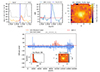 |
Fig. A.1. Example showing the S/N in datacubes. Upper Panel: S/N derived from the integrated spectra. From left to right are presented: integrated spectrum of the flux (yellow) and noise (gray) as a function of wavelength, the S/N as a function of wavelength, and the collapsed Hα image. To compute the continuum and S/N from the integrated spectra of Hα-emission, we utilized the gauss_fit module from MPDAF library, which provides the Gaussian-fit, flux at the peak emission, and average continuum. The Gaussian fit is represented by the red dashed line in the spectrum plot (first panel), and the S/N around the Hα-peak is specified in the legend of the S/N plot (middle panel). Here, we computed the S/N value with in λHα ± 0.005μm, which approximately covers the Gaussian of Hα flux. Lower Panel: S/N derived from the 1D spectra of the datacube, with blue denoting the full Hα cube and red indicating the masked region (i.e., identified Hα emission). Additionally, in same panel, we show the distribution of S/N in the mask and the collapsed Hα images, left and right small windows, respectively. We compare the S/N of the integrated spectra (upper row, middle panel) with the S/N distribution of 1D spectra (lower panel, left zoom-in window). Throughout the analysis, we observe that the average S/N of the 1D spectra is approximately similar to the value obtained from the integrated spectra. This justifies our S/N measurement techniques. |
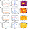 |
Fig. A.2. Example of quality assessment of KMOS3D and KGES sample. Row 1 & 2 shows Q1 and Q2 galaxies, respectively, Row 3 & 4 are Q3 galaxies. The color codes are given in the legend of the plots. |
Appendix B: Constraining gas geometrical parameters with 3DBarolo
As we go higher in redshift the information on morphological gas central x-y position (xc, yc) and position angle (PA) starts differentiating from their photometric measurements (as reported in Wisnioski et al. 2015; Harrison et al. 2017; Sharma et al. 2021a). On the other hand, from our previous work with 3DBarolo (Sharma et al. 2021a), we learned that 3DFIT TASK is not feasible in constraining the multiple parameters. Therefore, in this work we estimate gas geometrical parameters using an optimization function that runs atop of 3DBarolo run. This optimization function takes following inputs: (1) loss function given in Eq. 3, (2) Initial guess and bounds on parameter to be fit, (3) minimization method, and (4) ‘par file’ to execute 3DBarolo run. In particular, we optimize PA, xc, and yc. Initial guess on these parameters comes from the photometric information or from Hα datacubes (discussed in Sec. 2). The bounds are as following: [xc = xphot ± 4, yc = yphot ± 4] and PA[0, 360]. To be accurate, we also optimize systemic velocity (Vsys), the initial gas on it is computed from ‘Doppler shift’ of Hα line, and bounds are [-200, 200]. However, choice of fitting Vsys is tricky, for example, when we observe high residuals in moment maps, we fix it to a median value given in 3DBarolo output files. The optimize-minimize function works in three steps:
-
Run 3DBarolo (free: Vrot, Vdisp, and in some cases Vsys), which gives moment maps, PV- diagrams, and estimates on Vrot and Vdisp.
-
Compute the loss function (Eq. 3). The data and model inputs in loss function depend on the choice of parameter to be fit, which we have discussed below.
-
Save the loss, and optimization log. The optimization log gives us the best estimate of parameters and success rate (True or False).
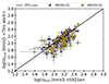 |
Fig. B.1. This figure compares the circular velocity of KROSS galaxies as computed in this study (y-axis) with that of Sharma et al. (2021b, x-axis). The Quality-1 and Quality-2 galaxies, as classified in Sharma et al. (2021a), are represented by yellow and purple circles, respectively, and the black line shows one-to-one relationship between two studies. |
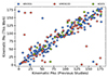 |
Fig. B.2. Comparison of kinematic PAs computed in this work with respect to previous studies. KROSS daste compared with Sharma et al. (2021a), KMOS3D with Wisnioski et al. (2019), and KGES with Tiley et al. (2021). The color codes are given in the legend of the plot. |
The optimization procedure follows a logical flow consists of four stages. Firstly, the xc and yc parameters are constrained using moment-0 maps, which provide information on the gas distribution. In the second stage, the previously optimized xc and yc positions are fixed to optimize the position angle (PA) parameter using minor axis PV diagrams. As noted in (Sharma et al. 2021a, appendix-A), the symmetry of the minor axis PV diagram around the axis indicates the correctness of the PA parameter; an asymmetric PV diagram implies an incorrect PA. In the third stage, the previously constrained xc, yc, and PA parameters are fixed to estimate the systemic velocity (Vsys) parameter. The loss function for Vsys uses major axis PV diagrams since Vsys directly affects the rotation velocity, which is determined by the major axis PV diagram. In the final stage, all optimized parameters are used to compute the final loss using moment-1 maps since our goal is to constrain the rotation velocity of the system. However, for cross-check, the final loss is also computed using moment-2 maps, although the difference is negligible (< 0.001) and does not appear in the residual maps. Lastly, the output corresponding to the minimum loss is saved.
We noted that this optimization procedure does not work for random guesses on the parameter values and requires reasonably close initial estimates, such as those provided by photometric estimates. Additionally, the procedure is computationally intensive, with each galaxy taking approximately 20-30 minutes to optimize when running on 8-cores. Nevertheless, this procedure is worthwhile for studying the nature of dark matter.
We evaluated the effectiveness of 3DBarolo+optimizer on the KROSS data, which we previously analyzed and discussed in Sharma et al. (2021a). As expected, the optimization process failed for galaxies with a low S/N (< 5), specifically those with Quality2. Consequently, we were compelled to exclude 56 out of 225 galaxies. In Figure B.1, we compare the circular velocities (computed at Rout) of KROSS sample, obtained with old and new kinematic modeling techniques. It is noteworthy that the previous and current circular velocity measurements are in reasonable agreement, with an intrinsic scatter of 0.03 dex. Both Quality-1 and Quality-2 galaxies in the GS21 sample exhibit variations in their circular velocities. Nonetheless, we used the new measurements because assessment of data-to-model fits in the PV diagram are better in the new analysis, as shown Figure E.4-E.9 uploaded at Zenodo (see section data availability). Moreover, moment-map residuals stays close to zero.
When we applied 3DBarolo and the optimizer on the KMOS3D and KGES dataset, we noticed that in some galaxies having moderate S/N levels (∼3 − 5), 3DBarolo was unable to identify the source mask, most-likely due to very noisy pixels. Additionally, for certain galaxies, the optimization of the position angle was unsuccessful, although the exact cause remains unknown. These instances were categorized under a batch of poor S/N (low-quality) galaxies for simplification purposes. In contrast, we notice that some galaxies with moderate signal-to-noise levels produced satisfactory results. This outcome may be attributed to the initial guess of the position angle closely aligning with the angle of the galaxy or relatively low noise in the unmasked pixels. It is important to acknowledge that these occurrences highlight the limitations of kinematic modeling. Therefore, our approach involves selecting results that are both available and reliable, i.e., where 3DBarolo yields reliable kinematic outputs and optimization demonstrate success.
To assess the reliability of the optimized parameters, specifically PAs, we compare the best-fit PAs with previously studied kinematic PAs: KROSS with Sharma et al. (2021a), KMOS3D with Wisnioski et al. (2019, PA received in private correspondance), and KGES with Tiley et al. (2021). As shown in Figure B.2, our estimates aligns very well with previous studies. Therefore, we concluded that 3DBarolo+optimizer works well on high-z moderate signal-to-noise data and hence can be used to constrain extra parameters.
Furthermore, we examined the maximum radius of rotation curves with respect to the PSF of final sample, see discussion in Section 3.4. As shown in Figure B.3, all the galaxies in final sample avid the criteria of Rmax > PSF. Therefore, this sample can easily be used for dynamical modeling and dark matter estimates.
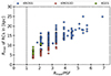 |
Fig. B.3. Rmax of rotation curves as a function of Rmax/PSF. |
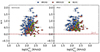 |
Fig. B.4. This figure shows the rotation to dispersion ratio (v/σ) of galaxies as a function of circular velocity computed at Rout. The left and right panels show v/σ before and after PGCs, respectively. The red horizontal dashed line indicates v/σ = 1.1. This figure demonstrates that, after pressure support corrections, all the galaxies are rotation-dominated. Therefore, we do not exclude any galaxies based on their observed v/σ values. |
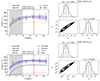 |
Fig. B.5. Examples of mass modeled rotation curves in the case of the maximum stellar disk scenario (upper panel) and maximum stellar+gas disk (lower panel). The best-fit parameters are shown in the right column, and color codes are given in the legend of the plot, where ‘MM’ stands for dynamical mass-model profiles estimated using Bayesian inference, and ‘fid’ stands for fiducial profile derived from given photometric mass. This example favors the maximum stellar and baryonic disk scenario, upper and lower panels, respectively. |
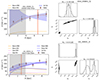 |
Fig. B.6. Examples of mass modeled rotation curves in the case of the maximum stellar disk scenario (upper panel) and maximum stellar+gas disk (lower panel). The best-fit parameters are shown in the right column, and color codes are given in the legend of the plot, where ‘MM’ indicates dynamical mass-model profiles estimated using Bayesian inference and ‘fid’ stands for the fiducial profile derived from a given photometric mass. This example demonstrates that (1) the model is incapable of fitting the observations using only baryons, and (2) the best-fit values for stellar or gas mass are an order of magnitude higher than their fiducial values, which is unrealistic given the uncertainties in the observations. Therefore, we suggest that the dark matter halo component is required in high-z galaxies. |
Appendix C: Mass modeling of rotation curves
Initially, we assume the absence of dark matter halos around high-z galaxies and dynamically model the baryonic component to fully fit the observed rotation curves. In this case, observed velocity is defined as
where Vstars represents the contribution of stars in both the bulge and disk, while Vgas encompasses the combined effect of molecular and atomic gas components. It is important to note that in the maximum stellar-disk scenario, the second term on the right-hand side of the equation becomes null.
We performed the dynamical modeling using a Bayesian inference technique established in Sharma et al. (2022), which employs flexible models. For Bayesian inference, we employed Markov chain Monte Carlo analysis, assuming a χ2 test statistic on observed kinematics and modeled kinematics. In our modeling approach, we assumed that the distribution of stars and gas follows an exponential mass profile (Freeman 1970), while the bulge is treated as a point mass. It is worth noting that the bulge remains unresolved in all datasets. Moreover, we only fit the outer rotation curves; therefore, we fixed the bulge mass at 109 M⊙ as a first-order approximation. To estimate the molecular and atomic gas masses, we use observed scaling relations, as described in Section 2.4, where we fixed the star-formation rate at its fiducial value. This approach allowed us to obtain realistic gas masses for a given stellar mass and star-formation rate. In the modeling, we kept flat priors on the stellar disk mass (8.0 ≤ log(Mstar M⊙)≤12.0) and kept a Gaussian prior with a 25% relative uncertainty for the stellar disk radius. A comprehensive discussion of this mass modeling technique can be found in Sharma et al. (2022, sec: 3.1).
In Figures B.5 and B.6, we provide a few examples of mass-modeled rotation curves (rotation curves) to illustrate different scenarios. The upper panel of Figure B.5 depicts the maximum stellar disk scenario, while the lower panel represents the maximum stars+gas disk scenario. The corresponding best-fit parameters are displayed in the right column. Figures B.5 demonstrates the robustness of our mass modeling technique. However, Figure B.6 reveals the limitations of using the same models, as we are unable to precisely constrain the stellar mass, whether considering the maximum stellar disk or the stars+gas disk scenario. In some cases depicted in the same figure (lower panel), the mass modeling allows for extremely high gas masses while suppressing the stellar masses to values lower than their observed photometric masses. Furthermore, we observe that the majority of the sample exhibits best-fit stellar masses that are an order of magnitude higher than their fiducial values (see Figure 9). These discrepancies are both alarming and unrealistic, indicating the probable necessity of an additional halo component in these galaxies.
Appendix D: Halo model independent fDM
In our previous work Sharma et al. (2021b), we established a halo model independent framework to study the dark matter fraction of high-z. In this framework, first we compute the total dynamical mass of galaxy directly from its rotation curve. The dynamical mass of a galaxy is defined as
where V(R) is the circular velocity computed at radius R and κ(R) is the geometric factor accounting for the presence of a stellar disk alongside the spherical bulge and halo (see, Persic & Salucci 1990). For Re, Ropt, and Rout, the values of κ are 1.2, 1.05, and 1.0, respectively (see also Sharma et al. 2021b). The bulge mass contribution within 5 kpc is negligible for local spirals; therefore, we do not model it. However, the geometric parameter κ(R) in the dynamical mass calculation takes into account the distribution of the mass located in the bulge and in the disk.
Second, we disentangled the contribution of total baryonic mass from dynamical mass.18 Briefly, we know that our samples are fair representative of main-sequence of star-forming galaxies as shown in Figure 3, which allowed us to compute their molecular and atomic masses using scaling relations (Tacconi et al. 2018; Chowdhury et al. 2022; Lagos et al. 2011, respectively). Our goal is to calculate the dark matter fraction of our galaxies within Re, Ropt, and Rout, and therefore we must first determine the baryonic masses within these radii. In (Sharma et al. 2021a), we found that rotation curves of z ∼ 1 galaxies are similar to local star-forming disk galaxies. This suggests that the radial distribution of stellar and molecular gas masses within these galaxies can be well approximated by the Freeman disk (Freeman 1970):
![$$ \begin{aligned} \begin{array}{r@l} V_{\mathrm{star}}^2(R) = \frac{1}{2} \Big ( \frac{GM_{\mathrm{star}}}{R_{\mathrm{star}}} \Big ) \ \Big ( \alpha \frac{R}{R_{\mathrm{star}}} \Big )^2 \ [I_0K_0 - I_1K_1], \\ V_{\mathrm{H2}}^2(R) = \frac{1}{2} \Big ( \frac{GM_{\mathrm{H2}}}{R_{\mathrm{H2}}} \Big ) \ \Big ( \alpha \frac{R}{R_{\mathrm{H2}}} \Big )^2 \ [I_0K_0 - I_1K_1],\\ V_{\mathrm{HI}}^2(R) = \frac{1}{2} \Big ( \frac{GM_{\mathrm{HI}}}{R_{\mathrm{HI}}} \Big ) \ \Big ( \alpha \frac{R}{R_{\mathrm{HI}}} \Big )^2 \ [I_0K_0 - I_1K_1], \end{array} \end{aligned} $$](/articles/aa/full_html/2025/07/aa47922-23/aa47922-23-eq18.gif)
where M_ and Rscale are the total mass and the scale length of the different components (stars, H2, and HI), respectively, and In and Kn are modified Bessel functions computed at α = 1.6 for stars and α = 0.53 for gas (c.f. Persic et al. 1996; Karukes & Salucci 2017). In this scenario, stars are assumed to be distributed in the stellar disk (R* = RD) known from photometry, discussed in Section [2]. The molecular gas is generally distributed outward through the stellar disk (up to the length of the ionized gas Rgas); therefore, we take RH2 ≡ Rgas. Here, we estimate the gas scale length Rgas by fitting the Hα surface brightness, see Sharma et al. (2021b, see appendix-C). Moreover, studies of local disk galaxies have shown that the surface brightness of the HI disk is much more extended than that of the H2 disk (Fu et al. 2010, see their Fig. 5); see also Leroy et al. (2008) and Cormier et al. (2016). Therefore, we assume RHI = 2 × RH2, which is a rough estimate, but still reasonable, considering that at high-z no information is available on the MHI (or MH2) surface brightness distribution. Thus, the Equation [D.2] allowed us to estimate M*, MHI, and MH2 within different radii (Re, Ropt, and Rout) using spherical symmetry (M(< R) = V2 × R/G).
Given the information on bayonic and dynamical masses, the dark matter fractions within radius R can be computed as
Therefore, using Equation[D.3], we computed fDM within Re, Ropt, and Rout for all three datasets. We note that, owing to the limited spatial resolution in our rotation curves, the measurements of fDM within Re are less accurate than for Ropt and Rout.
The stellar disk in high-z galaxies is often unresolved, making it difficult to determine whether the disk follows an exponentially thin profile (well described by Freeman 1970) or a thicker structure better modeled by a Sérsic profile (Sérsic 1963). To address this uncertainty, we estimate the stellar mass within a characteristic scale radius (e.g., Rout) using both the Sérsic profile (Sérsic 1963) and the Freeman disk (Freeman 1970). We adopt a Sérsic index of n = 1.35, which represents the average value for KROSS sample. The results are presented in Figure D.1. We find that assuming a Freeman disk yields stellar masses that are, on average, 1.02 times (≈0.21 dex) higher than those obtained using the Sérsic profile. In ideal cases where dark matter dominates the total mass, this results in only a minor decrease in the estimated dark matter fraction.
However, a significant change in fDM would occur if the stellar or baryonic mass were increased by a much larger fraction of the total mass, by an order of magnitude (0.7–1 dex, i.e., a factor of five to ten), which is seen in some low dark matter fraction galaxies in our sample. This is most likely due to a high gas mass fraction or other systematic effects discussed in Section 5. Conversely, adopting a Sérsic profile with n > 1.5 would systematically shift the low dark matter fraction galaxies toward higher fDM values, especially, in the outskirts. However, for the majority of KMOS3D and KGES galaxies, published Sérsic indices are not available. Therefore, following our previous studies (Sharma et al. 2021b, 2022) and seen obvious disk morphology in high-resolution images of our sample, we assume that the stars (and gas) are well distributed according to the Freeman disk (Freeman 1970).
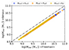 |
Fig. D.1. Comparison of stellar masses derived using Sérsic profile (y-axis) and Freeman disk (x-axis). Different color code are representing the different scale radii of galaxies within which stellar masses are estimated (blue: Rout, orange: Ropt, and yellow: Re), and black dotted-dashed line represents the one-to-one relation. |
Appendix E: Extra
E.1. Dark matter fraction within Ropt:
In Figure E.1, we plot the dark matter fraction within Ropt (∼2 Re) of galaxies as function of stellar mass. Firstly, we observe that the majority of the sample exhibits dark matter-dominated outer disks, with 23% of objects showing 0.2 ≤ fDM(< Ropt) < 0.5, and 36% of objects having fDM(< Ropt) < 0.2 (including objects in the forbidden region). Secondly, we notice a slightly decreasing trend of fDM as a function of stellar mass, except for a few outliers. Lastly, we compared the dark matter fraction within Ropt and Rout. Interestingly, we observed that galaxies generally exhibit slightly lower dark matter fractions in the inner region (Ropt) compared to outskirts (Rout). On average, dark matter fraction within Ropt is about 65%, while it is ∼75 − 80% within Rout, these finding coincides with the results reported in Sharma et al. (2021b).
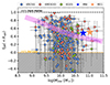 |
Fig. E.1. Dark matter fraction within Ropt. The KMOS3D, KGES, and KROSS datasets are represented in red, green, and blue colors, respectively. For comparison, we include two local massive disk galaxies: the Milky Way (MW) and Andromeda (M31), represented by the blue and the orange star, respectively. The solid black dashed line represents the 100% dark matter regime, while the yellow dashed line represents the baryon-dominated regime. The gray shaded area indicates the forbidden region, where galaxies with Mdyn < Mbar are located. |
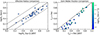 |
Fig. E.2. Left panel: Comparison of previously measured Re values of the KROSS sub-sample with the new JWST Re. The solid black line represents the one-to-one relation, while the dashed black lines indicate a scatter of 0.2 dex. Right panel: Dark matter fraction within Re using JWST photometry. Objects are color-coded based for their circular velocities within Re. |
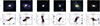 |
Fig. E.3. Hubble Space Telescope images and RCs of massive galaxies containing high dark matter fraction. That is, galaxies those are standing odd in fDM − Mstar relation. |
E.2. Improved Re measurements:
We had the opportunity to improve the measurement of Re for a subset of KROSS sample through the latest observations from the James Webb Space Telescope (JWST). This particular subset of galaxies is located within the COSMOS field (Skelton et al. 2014), which has recently been observed by the COSMOS-WEB team (Casey et al. 2023). For these targets JWST/NIRCam sizes in the filters F115W, F150W, F277W and F444W were recovered via Sérisc profile fitting using GALFITM (Häußler et al. 2013) with the same methodology outlined in Martorano et al. (2023) on mosaics publicly available in the Dawn JWST Archive19(Valentino et al. 2023). In this study, we employ the Re values obtained from the F115W band, which closely corresponds to the rest-frame Hα-wavelength observed at z ∼ 0.85.
In Figure E.2, the left panel illustrates the comparison between the new JWST-derived Re and the previously measured Re adopted from KROSS parent catalog. We observe that the JWST Re values are higher than the previous measurements but remain within a scatter of 0.2 dex. Although the difference is small, these newly improved Re measurements are crucial for investigating the dark matter fraction, especially within Re. Therefore, we have estimated the dark matter fraction using the updated Re values, as shown in the right panel of Figure E.2. We observe that galaxies with low dark matter fractions (< 20%) have been pushed toward higher values. In this specific sub-sample, none of the galaxies have a dark matter fraction below 20%.
All Tables
All Figures
|
Fig. 1. Distributions of the physical properties of the KMOS3D parent and selected sample, arranged from top-left to bottom-right: inclinations, stellar masses, effective radii, and redshifts. The dark blue histogram represents all Hα datacubes with confirmed spectroscopic redshift. The blue histogram shows Hα-detected galaxies with Flag-0 or Flag-1 in Table-6 of Wisnioski et al. (2019). We further select galaxies with inclination angles between 25° ≤θi ≤ 75°, shown in the sky-blue histogram. Lastly, we narrow our focus to galaxies with a signal-to-noise ratio greater than 3, depicted by the yellow hatched histogram. This selection criteria allowed us to perform the robust kinematic modeling of these high-z galaxies. |
| In the text | |
|
Fig. 2. Distributions of the physical properties of the KGES parent and selected samples, arranged from top-left to bottom-right: inclinations, stellar masses, effective radii, and redshifts. The dark blue histogram represents all Hα datacubes with confirmed spectroscopic redshift. The blue histogram shows Hα-detected galaxies (Tiley et al. 2021). We further select galaxies with inclination angles between 25° ≤θi ≤ 75°, which are shown in the sky-blue histogram. Lastly, we narrow our focus to galaxies with a signal-to-noise ratio greater than 3, depicted by the yellow hatched histogram. This selection criteria allowed us to perform the robust kinematic modeling of these high-z galaxies. |
| In the text | |
|
Fig. 3. Position of galaxies (final sample) with respect to the star-forming main sequence (MS). We plot offset from the MS, δMS (=SFR/SFR(MS; z, Mstar)) as a function of the stellar mass (Mstar) with the reference SFR(MS; z, Mstar) from Speagle et al. (2014). The gray shaded area represents the typical limit (0.3 dex) of star-forming MS (e.g., see Rodighiero et al. 2011; Genzel et al. 2015; Tacconi et al. 2018; Freundlich et al. 2019). The KMOS3D, KGES, and KROSS data are denoted by red, green, and blue filled circles, respectively. The solid lines in corresponding colors depict the average offset from the main sequence for each dataset. All galaxies are within 2σ scatter of the MS line. The galaxies marked with stars are the galaxies that have Re > PSF. |
| In the text | |
|
Fig. 4. Distributions of the physical properties of galaxies after kinematic modeling, arranged from top-left to bottom-right: inclinations, stellar masses, effective radii, and redshifts. These distributions are presented for the KMOS3D (in red), KGES (in green), and KROSS (in blue) samples. In total, we use 73 KMOS3D, 21 KGES, and 169 KROSS galaxies to estimate the DM fraction at high-z. The distribution of Re > PSF galaxies (within final sample) is shown by black hatched histograms. For detailed information on sample selection following kinematic modeling, we refer the reader to Section 3.2. |
| In the text | |
|
Fig. 5. Outputs of the kinematic modeling of selected KMOS3D (red box), KGES (green), and KROSS (blue) sources obtained using 3DBAROLO. Row-1, Columns 1-3: Rotation velocity map data, model, and residuals, respectively. The gray dashed line shows the position angle, the black cross the central x-y position, and the green line marks the plane of rotation. Row-2, Columns 1-3: Velocity dispersion map data, model, and residuals, respectively. Column 4: Major axis PV diagram, where the black shaded area with blue contour represents the data while the red contour shows the model, and the orange squares with error bars are the best-fit line-of-sight rotation velocity inferred by 3DBAROLO. The yellow and blue vertical dashed lines represent the effective radius (Re), and the optical radius (Ropt = 1.89 Re), respectively. Column 5: Corresponding velocity dispersion curve. The first point in the rotation and dispersion curves is represented by an empty (or white) marker, as it falls under the resolution limit and is therefore excluded from the data analysis. |
| In the text | |
|
Fig. 6. Impact of the pressure gradient on the circular velocity of galaxies computed at Rout. The KMOS3D, KGES, and KROSS samples are denoted by red circles, green cross, and blue stars, respectively. The interior of each data point is color-coded for rotation-to-dispersion ratio computed before pressure support correction ( |
| In the text | |
|
Fig. 7. Stellar masses as a function of ratio between PSF/Re. The KMOS3D, KGES, and KROSS samples are represented by red circles, green crosses, and blue stars, respectively, with a vertical dashed line indicating PSF = xRe. This figure indicates that only a limited number (= 53) of galaxies are applicable for determining the dark matter fraction within Re. However, it is important to note that our analysis is not restricted within Re. In fact, we evaluate the dark matter fraction at outer radii (i.e., R > Re). |
| In the text | |
|
Fig. 8. Cumulative distribution of the ratio between the last observed radius in the rotation curves (Rlast) and the effective radius (Re). The yellow, blue, and gray dashed lines indicate the scale radii Re, Ropt, and Rout, respectively. This plot shows that for the entire sample, Rlast > Re, while approximately 83% and 67% of objects have Rlast greater than Ropt and Rout, respectively. |
| In the text | |
|
Fig. 9. Comparison of photometric (PHOT) stellar and baryonic (stars+gas) masses with mass-modeled stellar and baryonic masses in the case of the maximum stellar disk and maximum stellar+gas disk scenarios, upper and lower panels, respectively. The KMOS3D, KGES, and KROSS datasets are depicted in red, green, and blue colors, respectively. The dashed black line indicates when mass-modeled masses are equivalent to their fiducial values (i.e., photometric masses), suggesting that objects lying above this line require the presence of a dark matter halo. |
| In the text | |
|
Fig. 10. Dark matter fraction within Re as a function of stellar masses for galaxies having Re > PSF. The KMOS3D, KGES, and KROSS datasets are depicted in red, green, and blue colors, respectively. The errors on the datasets are 68% confidence intervals. For comparison, we include two local massive disk galaxies: the Milky Way (MW) and Andromeda (M31), represented by the blue and the orange star, respectively. Additionally, we compare these results with previous studies at high redshift, such as Genzel et al. (2017, yellow circles), Genzel et al. (2020, yellow hexagons), Nestor Shachar et al. (2023, yellow dots), Bouché et al. (2022, yellow star), Übler et al. (2018, yellow diamond), Drew et al. (2018, yellow cross), and Puglisi et al. (2023, purple triangle). The black square represents the two galaxies that are in-common with Genzel et al. (2020) drawn from this work, while pink hexagons shows the measurements of same objects from Genzel et al. (2020). The black and yellow horizontal dashed lines represent the regimes of 100% dark matter dominance and baryon dominance, respectively. The gray shaded area indicates the ‘forbidden’ region, where galaxies with Mdyn < Mbar are located. Horizontal histograms (aligned to the right y-axis) compare datasets: KMOS3D, KGES, and KROSS (filled red, green, and blue hists), Genzel et al. (2017, 2020) (yellow fill with solid brown line), Nestor Shachar et al. (2023) (yellow fill with dashed brown line), and Bouché et al. (2022) and Puglisi et al. (2023) (open histograms in green and purple, respectively). |
| In the text | |
|
Fig. 11. Dark matter fraction within Rout. The KMOS3D, KGES, and KROSS datasets are represented in red, green, and blue colors, respectively. The binned dark matter fraction, calculated using weighted mean and root-mean-square statistics discussed in Section 4.2, is represented by off-white and white color hexagons, respectively, connected by black lines. The uncertainties on individual and binned data points represent the 68% confidence interval. For comparison, we include two local massive disk galaxies: the Milky Way (MW) and Andromeda (M31), represented by the blue and the orange star, respectively. The pink shaded area represents local star-forming disks (Persic et al. 1996). The solid black dashed line represents the 100% dark matter regime, while the yellow dashed line represents the baryon-dominated regime. The gray shaded area indicates the ‘forbidden’ region, where galaxies with Mdyn < Mbar are located. These color codes are same throughout the text. |
| In the text | |
|
Fig. 12. Dark matter fraction across the cosmic time. Left panel: Dark matter fraction within Rout as a function of redshift. The color codes of datasets are same as Figure 11, and given in the legend of the plot. The gray stars represents the binned data points with 1σ uncertainty shown by error-bars. Right panel: Averaged dark matter fraction within Re, Ropt, and Rout as a function of redshift, represented by yellow and blue lines, respectively. The bootstrap-errors representing 68% confidence interval are indicated by shaded areas color-coded with the same color as the averaged line. Dark matter fraction of local star-forming galaxies within Ropt and Rout are from Persic et al. (1996), and within Re they are taken from disk galaxy survey of Courteau & Dutton (2015). The uncertainties on these measurements are, on average, ±0.25. The color code of these estimates are same as high-z galaxies. The dark-yellow dotted-dashed lines shows the dark matter fraction within Re from Nestor Shachar et al. (2023). |
| In the text | |
|
Fig. 13. Scaling relations of dark matter, fDM − Σbar and fDM − Vc, shown in the left and right panels, respectively. The blue dashed line represents the best fit to the data in both relations, with the associated intrinsic scatter (ζint) indicated on the plot. We note that the fDM − Vc relation can be seen as the result of a combination of the mass-velocity and mass-size relations. The color codes used for data in both panels are consistent with Figure 11. We note that the uncertainties on data points represent the 68% confidence interval. |
| In the text | |
|
Fig. 14. Exploration of the fDM − Σbar relation across different stellar masses and redshift intervals. First panel: fDM − Σbar relation for the low-stellar mass bin (Mstar ≤ 1010 M⊙) in yellow and the high-stellar mass bin (Mstar > 1010 M⊙) in orange. The original best-fit to fDM − Σbar relation is shown blue dashed line, while the best fit of low- and high-stellar mass bins are shown by brown and orange dashed lines, respectively. Second-third panel: fDM − Σbar relation separated for low- and high-stellar masses, left and right panels respectively. In both panels, low-z (z ≤ 1) and high-z (z > 1) galaxies are shown in blue and red, respectively, and corresponding best fits are shown in dark blue and red dashed-lines. In the first panel, median error on the data points is indicated by gray cross. The filled crosses & circles represent the measurements taken within Ropt and Rout, respectively. We note to the reader that these relations are plotted exclusively for objects with fDM > 0, while the full sample is shown in Figure 13. |
| In the text | |
|
Fig. 15. Exploration of the fDM − Vc relation across different stellar masses and redshift intervals. First panel: fDM − Vc relation for the low-stellar mass bin (Mstar ≤ 1010 M⊙) in yellow and the high-stellar mass bin (Mstar > 1010 M⊙) in orange. The best-fit to original fDM − Vc relation is shown blue dashed line given by Equation (6). The Equations corresponds to best fit of low- and high-stellar mass bins is written on the plot, shown by brown and orange dashed lines, respectively. The intrinsic scatter (ζint) associated with fits are printed on plot using same color code. Second-third panel: fDM − Vc relation separated for low- and high-stellar masses, left and right panel respectively. In both panels, low-z (z ≤ 1) and high-z (z > 1) galaxies are shown in blue and red, respectively, and corresponding best-fits are shown by dashed blue and red lines. In all panels, filled crosses and circles represent the measurements taken within Ropt and Rout, respectively, and median error on the data points is indicated by gray crosses. Low surface brightness and low velocity low mass galaxies at high redshift might be missed from the sample. On the other hand, it is clear that DM fractions are lower at fixed rotational velocity at higher redshift, i.e. the plots are not biased on the vertical axis. We note to the reader that these relations are plotted exclusively for objects with fDM > 0 for the clarity on the matter, while the full sample is shown in Figure 13. |
| In the text | |
|
Fig. A.1. Example showing the S/N in datacubes. Upper Panel: S/N derived from the integrated spectra. From left to right are presented: integrated spectrum of the flux (yellow) and noise (gray) as a function of wavelength, the S/N as a function of wavelength, and the collapsed Hα image. To compute the continuum and S/N from the integrated spectra of Hα-emission, we utilized the gauss_fit module from MPDAF library, which provides the Gaussian-fit, flux at the peak emission, and average continuum. The Gaussian fit is represented by the red dashed line in the spectrum plot (first panel), and the S/N around the Hα-peak is specified in the legend of the S/N plot (middle panel). Here, we computed the S/N value with in λHα ± 0.005μm, which approximately covers the Gaussian of Hα flux. Lower Panel: S/N derived from the 1D spectra of the datacube, with blue denoting the full Hα cube and red indicating the masked region (i.e., identified Hα emission). Additionally, in same panel, we show the distribution of S/N in the mask and the collapsed Hα images, left and right small windows, respectively. We compare the S/N of the integrated spectra (upper row, middle panel) with the S/N distribution of 1D spectra (lower panel, left zoom-in window). Throughout the analysis, we observe that the average S/N of the 1D spectra is approximately similar to the value obtained from the integrated spectra. This justifies our S/N measurement techniques. |
| In the text | |
|
Fig. A.2. Example of quality assessment of KMOS3D and KGES sample. Row 1 & 2 shows Q1 and Q2 galaxies, respectively, Row 3 & 4 are Q3 galaxies. The color codes are given in the legend of the plots. |
| In the text | |
|
Fig. B.1. This figure compares the circular velocity of KROSS galaxies as computed in this study (y-axis) with that of Sharma et al. (2021b, x-axis). The Quality-1 and Quality-2 galaxies, as classified in Sharma et al. (2021a), are represented by yellow and purple circles, respectively, and the black line shows one-to-one relationship between two studies. |
| In the text | |
|
Fig. B.2. Comparison of kinematic PAs computed in this work with respect to previous studies. KROSS daste compared with Sharma et al. (2021a), KMOS3D with Wisnioski et al. (2019), and KGES with Tiley et al. (2021). The color codes are given in the legend of the plot. |
| In the text | |
|
Fig. B.3. Rmax of rotation curves as a function of Rmax/PSF. |
| In the text | |
|
Fig. B.4. This figure shows the rotation to dispersion ratio (v/σ) of galaxies as a function of circular velocity computed at Rout. The left and right panels show v/σ before and after PGCs, respectively. The red horizontal dashed line indicates v/σ = 1.1. This figure demonstrates that, after pressure support corrections, all the galaxies are rotation-dominated. Therefore, we do not exclude any galaxies based on their observed v/σ values. |
| In the text | |
|
Fig. B.5. Examples of mass modeled rotation curves in the case of the maximum stellar disk scenario (upper panel) and maximum stellar+gas disk (lower panel). The best-fit parameters are shown in the right column, and color codes are given in the legend of the plot, where ‘MM’ stands for dynamical mass-model profiles estimated using Bayesian inference, and ‘fid’ stands for fiducial profile derived from given photometric mass. This example favors the maximum stellar and baryonic disk scenario, upper and lower panels, respectively. |
| In the text | |
|
Fig. B.6. Examples of mass modeled rotation curves in the case of the maximum stellar disk scenario (upper panel) and maximum stellar+gas disk (lower panel). The best-fit parameters are shown in the right column, and color codes are given in the legend of the plot, where ‘MM’ indicates dynamical mass-model profiles estimated using Bayesian inference and ‘fid’ stands for the fiducial profile derived from a given photometric mass. This example demonstrates that (1) the model is incapable of fitting the observations using only baryons, and (2) the best-fit values for stellar or gas mass are an order of magnitude higher than their fiducial values, which is unrealistic given the uncertainties in the observations. Therefore, we suggest that the dark matter halo component is required in high-z galaxies. |
| In the text | |
|
Fig. D.1. Comparison of stellar masses derived using Sérsic profile (y-axis) and Freeman disk (x-axis). Different color code are representing the different scale radii of galaxies within which stellar masses are estimated (blue: Rout, orange: Ropt, and yellow: Re), and black dotted-dashed line represents the one-to-one relation. |
| In the text | |
|
Fig. E.1. Dark matter fraction within Ropt. The KMOS3D, KGES, and KROSS datasets are represented in red, green, and blue colors, respectively. For comparison, we include two local massive disk galaxies: the Milky Way (MW) and Andromeda (M31), represented by the blue and the orange star, respectively. The solid black dashed line represents the 100% dark matter regime, while the yellow dashed line represents the baryon-dominated regime. The gray shaded area indicates the forbidden region, where galaxies with Mdyn < Mbar are located. |
| In the text | |
|
Fig. E.2. Left panel: Comparison of previously measured Re values of the KROSS sub-sample with the new JWST Re. The solid black line represents the one-to-one relation, while the dashed black lines indicate a scatter of 0.2 dex. Right panel: Dark matter fraction within Re using JWST photometry. Objects are color-coded based for their circular velocities within Re. |
| In the text | |
|
Fig. E.3. Hubble Space Telescope images and RCs of massive galaxies containing high dark matter fraction. That is, galaxies those are standing odd in fDM − Mstar relation. |
| In the text | |
Current usage metrics show cumulative count of Article Views (full-text article views including HTML views, PDF and ePub downloads, according to the available data) and Abstracts Views on Vision4Press platform.
Data correspond to usage on the plateform after 2015. The current usage metrics is available 48-96 hours after online publication and is updated daily on week days.
Initial download of the metrics may take a while.