| Issue |
A&A
Volume 689, September 2024
|
|
|---|---|---|
| Article Number | A318 | |
| Number of page(s) | 18 | |
| Section | Extragalactic astronomy | |
| DOI | https://doi.org/10.1051/0004-6361/202348667 | |
| Published online | 23 September 2024 | |
Tully-Fisher relation of late-type galaxies at 0.6 ≤ z ≤ 2.5
1
Observatoire Astronomique de Strasbourg, Université de Strasbourg, CNRS UMR 7550, 67000 Strasbourg, France
2
University of Strasbourg Institute for Advanced Study, 5 allée du Général Rouvillois, 67083 Strasbourg, France
3
Department of Physics and Astronomy, University of the Western Cape, Cape Town 7535, South Africa
4
INFN-Sezione di Trieste, Via Valerio 2, 34127 Trieste, Italy
5
IFPU Institute for Fundamental Physics of the Universe, Via Beirut, 2, 34151 Trieste, Italy
6
SISSA International School for Advanced Studies, Via Bonomea 265, 34136 Trieste, Italy
7
Department of Physics, Indian Institute of Technology, Hyderabad, Telangana 502284, India
Received:
19
November
2023
Accepted:
13
June
2024
We present a study of the stellar and baryonic Tully-Fisher relation within the redshift range of 0.6 ≤ z ≤ 2.5, utilizing observations of star-forming galaxies. This dataset comprises of disk-like galaxies spanning a stellar mass range of 8.89 ≤ log(Mstar [M⊙]) ≤ 11.5, a baryonic mass range of 9.0 ≤ log(Mbar [M⊙]) ≤ 11.5, and a circular velocity range of 1.65 ≤ log(Vc [km/s]) ≤ 2.85. We estimated the stellar masses of these objects using spectral energy distribution fitting techniques, while the gas masses were determined via scaling relations. Circular velocities were directly derived from the rotation curves (RCs), after meticulously correcting for beam smearing and pressure support. Our analysis confirms that our sample adheres to the fundamental mass-size relations of galaxies and reflects the evolution of velocity dispersion in galaxies, in line with previous findings. This reaffirms the reliability of our photometric and kinematic parameters (i.e., Mstar and Vc), thereby enabling a comprehensive examination of the Tully-Fisher relation. To attain robust results, we employed a novel orthogonal likelihood fitting technique designed to minimize intrinsic scatter around the best-fit line, as required at high redshifts. For the stellar Tully-Fisher relation, we obtained a slope of α = 3.03 ± 0.25, an offset of β = 3.34 ± 0.53, and an intrinsic scatter of ζint = 0.08 dex. Correspondingly, the baryonic Tully-Fisher relation yielded α = 3.21 ± 0.28, β = 3.16 ± 0.61, and ζint = 0.09 dex. Our findings indicate a subtle deviation in the stellar and baryonic Tully-Fisher relation with respect to local studies, which is most likely due to the evolutionary processes governing disk formation.
Key words: galaxies: evolution / galaxies: high-redshift / galaxies: kinematics and dynamics
© The Authors 2024
 Open Access article, published by EDP Sciences, under the terms of the Creative Commons Attribution License (https://creativecommons.org/licenses/by/4.0), which permits unrestricted use, distribution, and reproduction in any medium, provided the original work is properly cited.
This article is published in open access under the Subscribe to Open model. Subscribe to A&A to support open access publication.
1. Introduction
Scaling relations in galaxies refer to the empirical correlations between a range of observable properties, such as luminosity, mass, size, and rotational velocity. These relations offer invaluable insights into the fundamental physics and evolutionary dynamics shaping galaxies, thereby serving as rigorous benchmarks against which theoretical models of galaxy formation and evolution are tested. Among the various scaling relations, the Tully-Fisher relation holds a place of particular significance in galaxy evolution and cosmology. This correlation acts as an analytical cornerstone, unraveling the complexities of galaxy dynamics and morphology and deepening our understanding of the interplay among the physical properties of galaxies.
In the realm of galaxy dynamics, the Tully-Fisher relation (TFR) is one of the most studied empirical scaling relations that correlates the properties of luminous matter with those of the dark halo. In the traditional TFR, which originated from the seminal work of Tully & Fisher (1977), the luminosity of galaxies scales with their characteristic velocity (i.e., circular velocity Vc) via a power-law, L ∝ βVcα, where α is the slope, and β is the intercept in the relation. The slope indicates the extent of the circular velocity’s dependency on the luminosity, while the quantity β/α represents the zero point, which indicates the origin of the relation. In the Local Universe, this relation is remarkably tight (α ∼ 4, β/α ∼ 2, σint ≲ 0.1 dex) for star-forming disk galaxies (Tully & Fisher 1977; Feast 1994; Bell & de Jong 2001; Karachentsev et al. 2002; Pizagno et al. 2007; Toribio et al. 2011; McGaugh et al. 2000; Sorce et al. 2013). Consequently, it is widely used in redshift-independent distance measurements (Giovanelli et al. 1997b; Ferrarese et al. 2000; Freedman et al. 2011; Sorce et al. 2013; Neill et al. 2014); for example, knowing the luminosity and flux (L and F), we can relate the observed flux to the distance, (D), of the object via F ∝ L/4πD2. Furthermore, the TFR has played a significant role in determining cosmological parameters, particularly by enabling the measurement of the Hubble constant H0 out to the Local Universe (Giovanelli et al. 1997a; Tully & Pierce 2000; Masters et al. 2006).
The TFR serves not only as a distance indicator in cosmology, but also as a powerful tool for understanding the complex interaction between dark and luminous matter in galaxies. This is substantiated by a diverse range of observations (Mathewson et al. 1992; McGaugh et al. 2000; McGaugh 2005; Papastergis et al. 2016; Lapi et al. 2018) and simulations (Mo & Mao 2000; Steinmetz & Navarro 1999). The underlying rationale lies in the relationship between the circular velocity and the total gravitational potential of a galaxy, coupled with the luminosity serving as a tracer for the total stellar mass (Blumenthal et al. 1984; Mao et al. 1998; Girardi et al. 2002). An interaction between these physical quantities is manifested as a correlation, thus giving rise to the well-known TFR. This foundational concept has also led to a generalized form of the TFR, expressed as M ∝ βVcα, where M represents the galaxy’s stellar or baryonic mass. This generalized TFR has undergone extensive study and exhibits remarkable tightness, particularly in the Local Universe (Verheijen & Sancisi 2001; McGaugh 2005; de Blok et al. 2008; Stark et al. 2009; Foreman & Scott 2012; Lelli et al. 2016; Papastergis et al. 2016; Lapi et al. 2018; Lelli et al. 2019).
A note of caution is warranted when discussing the generalized TFR. In optical and infrared astronomy, luminosity primarily serves as a proxy for stellar mass, giving rise to the stellar Tully-Fisher relation (STFR). Conversely, at radio wavelengths, luminosity predominantly traces the mass of neutral hydrogen gas. When combined with the stellar mass, this provides an approximation of the total baryonic mass of a galaxy, Mbar ∝ Mstar + Mgas, thereby leading to the baryonic Tully-Fisher relation (BTFR). It is noteworthy that the slope of the BTFR closely resembles that of the seminal TFR, with a typical value around 4 and an intrinsic scatter below 0.1 dex (e.g., Lelli et al. 2019). In contrast, the slope of the STFR generally ranges between 3 and 3.5 – depending on the wavelength range, accompanied by a larger intrinsic scatter of approximately ∼0.25 dex (e.g., Lapi et al. 2018).
A number of previous studies have investigated the seminal and generalized TFR of star-forming galaxies (SFGs) in cluster environments (Ziegler et al. 2002; Böhm et al. 2004; van Starkenburg et al. 2006). These studies suggest that the slope of the TFR at intermediate redshifts (z ∼ 0.5) is shallower compared to local measurements, which has prompted discussions on potential selection bias effects (Avila-Reese et al. 2008; Gurovich et al. 2010; Williams et al. 2010; Mercier et al. 2022; Catinella et al. 2023). However, other studies have reported little to no evolution in the seminal TFR slope from z ∼ 1 to z ≈ 0 (Conselice et al. 2005; Kassin et al. 2007; Puech et al. 2010; Miller et al. 2011; Torres-Flores et al. 2011; Zaritsky et al. 2014; Abril-Melgarejo et al. 2021; Vergani et al. 2012; McGaugh & Schombert 2015). Other high-z studies, utilizing state-of-the-art integral field unit (IFU) observations of isolated SFGs (Puech et al. 2008; Gnerucci et al. 2011; Tiley et al. 2016; Übler et al. 2017) have found mixed results. We note, however, that most of these works have mainly focused on the evolution of the TFR zeropoint compared to the Local Universe values after assuming a fixed slope. Puech et al. (2008) found that the slope in K-band TFR at z ∼ 0.6 is consistent with the local value after allowing the slope to vary. Gnerucci et al. (2011) found a large scatter in the TFR at z ∼ 3; consequently, these authors used a fixed slope having the value same as that of the Local Universe. Tiley et al. (2016) studied the K-band TFR at z ∼ 1. They fit the TFR using both a fixed slope (obtained from the Local Universe value) as well as keeping it as a free parameter. When the slope was kept as a free parameter, significant differences were found compared to the Local Universe value (cf. Table 3 of Tiley et al. 2016). Übler et al. (2017) studied the stellar and baryonic TFR at redshifts z ∼ 0.9 and z ∼ 2.3 by using a fixed slope (fixed to the value in Lelli et al. 2016) and looking for the variation of zeropoint with redshift.
A whole bunch of studies have also been carried out on the stellar TFR (Kassin et al. 2007; Cresci et al. 2009; Puech et al. 2010; Williams et al. 2010; Torres-Flores et al. 2011; Vergani et al. 2012; Tiley et al. 2016; Price et al. 2016; Harrison et al. 2017; Pelliccia et al. 2017; Übler et al. 2017; Abril-Melgarejo et al. 2021; Catinella et al. 2023). In addition to fitting for the stellar TFR slope, many works have also assumed a constant slope and evaluated the scatter (Cresci et al. 2009; Price et al. 2016; Übler et al. 2017). Searches for an abrupt transition in the TFR slope using low redshift data have also been carried out, with null results reported (Krishak & Desai 2022).
Here, it is important to note that the early IFU studies have inherent uncertainties, primarily due to their 1D or 2D kinematic modeling approaches (as reported by Teodoro & Fraternali 2015). This is because telescopes equipped with IFUs can achieve only a spatial resolution of 0.5 − 1.0″, while a galaxy at z ∼ 1 typically has an angular size ranging from 2″ − 3″. As a result, a finite beam size leads to smearing of the line emission across adjacent pixels. Consequently, the gradient in the velocity fields tends to become flattened, and the line emission begins to broaden, creating a degeneracy in the calculation of rotation velocity and velocity dispersion. This observational effect is referred to as “beam smearing”, which affects the kinematic properties of galaxies by underestimating the rotation velocity and overestimating the velocity dispersion. Therefore, it is essential to model the kinematics in 3D space, taking into account the beam smearing on a per-spaxel basis. Recent studies by Di Teodoro et al. (2016), Sharma et al. (2021), and Sharma et al. (2023) have modeled the kinematics of high-z galaxies in 3D space and demonstrated significant improvements in overall kinematics, including 2D velocity maps and position-velocity diagrams (i.e., observed rotation curves). It is noteworthy that although some of the other high-z TFR studies have accounted for beam-smearing in the forward-modeling approach, none of them have have fitted for kinematics in full 3D space, similarly to the works of Di Teodoro et al. (2016) and Sharma et al. (2023).
Moreover, at high-z, the interstellar medium (ISM) in galaxies is highly turbulent (Burkert et al. 2010; Wellons et al. 2020). This turbulence within the ISM generates a force that counteracts gravity in the galactic disk via a radial gradient, which in turn suppresses the rotation velocity of gas and stars. This phenomenon is commonly referred to as “asymmetric drift” for the stellar component and “pressure gradient” for the gas component, as defined in Sharma et al. (2021). While the latter effect is generally negligible in local rotation-dominated galaxies (i.e., late-type galaxies), it is significantly observed in local dwarf and early-type galaxies (Valenzuela et al. 2007; Read et al. 2016; Weijmans et al. 2008). The highly turbulent conditions of the ISM and the dominance of gas at high-z (Turner et al. 2017; Johnson et al. 2018; Wellons et al. 2020) makes their velocity dispersion variable and anisotropic across galactic scales (Kretschmer et al. 2021). Consequently, the observed rotation velocity measurements are underestimated throughout the galactic radius and we may even observe a decline in the shape of rotation curves at high-z (Genzel et al. 2017; Sharma et al. 2021).
We point out that among the aforementioned high-z TFR studies, only Übler et al. (2017) has accounted for pressure gradient corrections by assuming a constant and isotropic velocity dispersion. However, recent studies of high-redshift observations (Sharma et al. 2021) and simulations (Kretschmer et al. 2021) indicate that pressure support corrections under the assumption of constant and isotropic velocity dispersion can lead to an overestimation of the circular velocities. This is particularly relevant for galaxies with low rotation-to-dispersion ratios (v/σ < 1.5). Given these findings, there is a compelling need to re-examine the TFR at high redshifts, employing more precise kinematic measurements as recommended in Di Teodoro et al. (2016), Sharma et al. (2021), and Kretschmer et al. (2021).
This study aims to revisit and refine our understanding of the TFR at high redshifts. Specifically, we utilize a large dataset recently analyzed by Sharma et al. (2023), which models the kinematics using 3D forward modeling and incorporates the pressure gradient while allowing for varying and non-isotropic velocity dispersion. The aim of this work is to investigate the cosmic-evolution of TFR in star-forming galaxies– disk-like systems, within the redshift range of 0.6 ≤ z ≤ 2.5. We focus on disk-like systems since they form and evolve predominantly at z ≤ 1.5 and exhibit homogeneous and controlled evolution (e.g., Lagos 2017). Thus, these systems serve as a valuable tool to infer the cosmic evolution of baryons and dark matter. At z ≈ 1, nearly 50% of the Universe’s stellar mass assembles in galactic halos (Pérez-González et al. 2008), and this marks the peak of cosmic star-formation density (Madau & Dickinson 2014, and references therein). Therefore, it is crucial to compare the baryonic and dark matter properties of galaxies at 0.6 ≤ z ≤ 2.5 with those in the Local Universe. This comparison provides insights into (1) the evolution of disk-like systems after their formation at z ≤ 1.5 and (2) the nature of dark matter because these systems are (more or less) in dynamical equilibrium.
This paper is organized as follows. In Section 2, we discuss the dataset, relevant parameters of STFR and BTFR relations, and we assess the quality of these parameters using fundamental scaling relations. In Sect. 3, we present the STFR and BTFR relations. In Sect. 4, we discuss these relations in comparison with previous studies. Finally, in Sect. 5 we summarize our work and present our main findings. In this work, we have assumed a flat ΛCDM cosmology with Ωm, 0 = 0.27, ΩΛ, 0 = 0.73 and H0 = 70 km s−1Mpc−1.
2. Data
For the purposes of this study, we made use of the dataset recently examined by Sharma et al. (2023, hereafter GS23). As discussed in GS23, this sample was initially selected based on the assessment of kinematic modeling outputs. In brief, kinematic modeling was based on the following primary criteria: (1) confirmed Hα detection and spectroscopic redshift, (2) inclination angles within the range of 25° ≤θi ≤ 75°, and (3) signal-to-noise ratio, S/N > 3 (in Hα datacubes). GS23 employed the 3DBarolo code to model the kinematics, allowing for beam smearing corrections and inclination within a 3D space. This results in velocity maps, major and minor axis position-velocity (PV) diagrams, surface brightness curves, rotation curves, and velocity dispersion curves. Following the kinematic modeling outcomes GS23 implemented secondary selection criteria, according to which galaxies were excluded if they met the following conditions: (1) 3DBarolo run did not succeed; (2) No mask was created, implying 3DBarolo’s failure to mask the true emission due to a moderate signal-to-noise; (3) maximum observed radius smaller than the point spread function, namely, Rmax < PSF, indicating 3DBarolo’s inability to create rings and hence fails to produce kinematic models; and (4) Rmax = PSF, in this case resulting kinematic models provide only two measurements in rotation curves, which were insufficient for dynamical modeling or reliable measurements of circular velocities. This secondary selection criteria resulted in a final sample of 263 galaxies, comprising 169 from KROSS, 73 from KMOS3D, and 21 from KGES. For the distribution of relevant physical quantities of the final sample we refer to Sharma et al. (2023, Fig. 4).
The rotation curves inferred from 3DBarolo are further corrected for pressure support through the “pressure gradient correction,” method as established by Sharma et al. (2021), and referred to as intrinsic rotation curves. We utilized these intrinsic rotation curves to estimate the circular velocities (Vc) of galaxies. The velocity dispersion (σ) is an average value estimated from velocity dispersion curves obtained from 3DBarolo; for more details, we refer to Sharma et al. (2021) and Sharma et al. (2023). GS23 sample spans a stellar mass range of 8.89 ≤ log(Mstar [M⊙]) ≤ 11.5, effective radii −0.2 ≤ log(Re [kpc]) ≤ 0.85, star formation rates between 0.49 ≤ log(SFR [M⊙ yr−1]) ≤ 2.5, and a redshift range of 0.6 ≤ z < 2.5. This sample is a fair representative of main-sequence star-forming galaxies, shown in Fig. 1. In the subsequent sections, we briefly examine the circular velocity and velocity dispersion estimates, discuss the baryonic mass estimates, and justify the accuracy of photometric and kinematic properties relevant for TFR study.
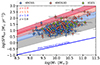 |
Fig. 1. Main sequence of local star-forming galaxies is shown by solid blue line and for redshifts of 1.0, 1.5, and 2.0, shown by blue, pink, and red shaded areas, respectively. The KMOS3D, KGES and KROSS data is shown by red, green, and blue filled circles. Hereafter, we refer this to full dataset as GS23 and depict in blue color throughout the work. |
2.1. Velocity measurements
In this study, we have examined the circular velocity of rotation curves at three distinct scale lengths, specifically Re, Ropt, and Rout (≈5 RD), which we denote as VcRe, VcRopt, and VcRout, respectively1. It is worth noting that the effective radius for the majority of our sample falls below the resolution limit, which is approximately 4.0 kpc with a median seeing of 0.5″. On the other hand, the optical radius remains on the verge of resolution limit. Thus, in order to be conservative, we only utilized circular velocity measurements that were obtained at Rout. This is one of the reasons of not plotting TFR for Vc(2.2RD) as adopted in previous studies (e.g., Übler et al. 2017; Tiley et al. 2019). However, the choice of Vc(2.2RD) aims to capture the flat portion of the rotation curves, akin to  in our case, which represents the circular velocity in the outer regions of the rotation curves assumed to be flat. Finally, it is important to remark that ∼92% and 65% of galaxy rotation curves are sampled up to Ropt and Rout, respectively. In cases where the rotation curve is not sampled up to the reference radius, we interpolate (or extrapolate) the velocity estimates. Our approach is as follows: (1) if Ropt exceeds Rlast (the maximum observed radius), Vc is computed at Rlast; and (2) if Rout > Rlast, Vc is computed at Ropt. This approach ensures that we remain within the outer regions of galaxies, which are assumed to have flat rotation curves based on local observations. We note that we did not interpolate (or extrapolate) the velocities beyond the maximum observed radius. Moreover, for interpolation, we did not employ any specific functional form of the rotation curve; instead, we utilized numpy.interp routine. This ensures that if the rotation curve is declining, it will continue to decline, and vice versa.
Additionally, it is worth noting that TFR studies in the Local Universe occasionally utilize the maximum velocity of the system (e.g., Lelli et al. 2019). Therefore, we also examined the maximum velocity in relation of VcRout. We extracted the maximum circular velocity (Vmax) from the rotation curves. We note that Vmax is not the asymptotic rotation velocity, hence, it involves no interpolation and extrapolation. The results of this comparison are presented in Fig. 2. Our analysis revealed a strong positive correlation of ∼97% between Vmax and VcRout, with an intrinsic scatter of 0.15 dex. Although we have observed that ∼30% of the sample exhibits Vmax values that are 0.1 dex higher than  , we consider to use
  as the circular velocity. The rationale behind this decision is the uncertainty in capturing the entire flat part of the rotation curves at high redshifts. As a result, Vmax might not accurately represent the maximum velocity of the galaxy. Hence, it cannot be compared with local or high-redshift studies. Therefore, to maintain uniformity across the sample, we treated all galaxies consistently and facilitated comparisons with previous high-redshift studies (e.g., Tiley et al. 2019; Übler et al. 2017), we have chosen to utilize VcRout as the circular velocity, hereafter, denoted as Vc.
 |
Fig. 2. Comparison of circular velocities, VcRout and Vmax. The black solid line shows the one-to-one relation followed by dashed lines showing the 1σ intrinsic scatter around this line. Since the measurements of VcRout and Vmax correlate within 1σ, it suggests that both velocity measurements are good proxies for circular velocity of galaxies. In the analysis, we refer to VcRout = Vc as the circular velocity of the object. |
In Fig. 3, we show the rotation-to-dispersion ratio of before and after pressure support corrected GS23 sample. The velocities before pressure support corrections are referred to as rotation velocity (Vrot), while after pressure support corrections its circular velocity (Vc) of the system. We notice that, prior to the implementation of pressure support corrections, there were only nine dispersion dominated galaxies (three KMOS3D, one KGES, and five KROSS). However, after applying pressure support corrections, none of these galaxies have Vc/σ < 1, as depicted in Fig. 3. Therefore, we did not exclude these galaxies from our analysis. Hence, the full GS23 sample is a good representative of rotation supported systems, which we employed to study TFR.
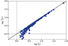 |
Fig. 3. Intrinsic and pressure-support-corrected rotation-to-dispersion ratio (V/σ), plotted on the y- and x-axes, respectively. The solid black line represents the one-to-one relation between the two quantities. The vertical and horizontal dashed lines indicate the V/σ > 1 limit for intrinsic and pressure-support-corrected rotation-to-dispersion ratios, respectively. This figure indicates that, after pressure support corrections, none of the GS23 galaxies exhibit dispersion-dominated characteristics. Therefore, we utilize the entire GS23 sample for the TFR study. |
We remark that underlying assumptions of GS23 consist of three key criteria: (1) galaxies should be located on or around the star-forming main sequence; (2) they should exhibit a disk-like morphology in high-resolution images, with no nearby neighbors within 150 kpc; and (3) the ratio of circular velocity to velocity dispersion: Vc/σ > 1. These three assumptions enable the selection of disk-like galaxies from high-z sample. Notably, our main findings in Sect. 3 are consistent with those of local studies (e.g., Lapi et al. 2018; Reyes et al. 2011), which generally select the star-forming galaxies with Vc/σ > 1. However, we notice that previous high-z studies apply higher Vrot/σ cuts to investigate the TFR, which we briefly discuss in Appendix C.
2.2. Baryonic masses
Observations show that typical star-forming galaxies lie on a relatively tight, almost linear, redshift-dependent relation between their stellar mass and star formation rate, the so-called main sequence of star formation (MS; e.g., Noeske et al. 2007; Whitaker et al. 2012; Speagle et al. 2014). Most stars since z ∼ 2.5 were formed on and around this MS (e.g., Rodighiero et al. 2011), and galaxies that constitute it, usually exhibit a rotating disk morphology (e.g., Förster Schreiber et al. 2006; Daddi et al. 2010; Wuyts et al. 2011). Figure 1 shows the position of the GS23 sample on the main sequence of typical star-forming galaxies (MS), the analytical prescription for the center of the MS as a function of redshift and stellar mass proposed in the compilation by Speagle et al. (2014), as a function of stellar mass. The figure shows that the all sources are on and around the main sequence between 0.65 ≤ z ≤ 2.5. A normalized main sequence plot of this dataset is shown in Sharma et al. (2023, Fig. 3). This suggests that GS23 sample is a good representative of disk-like star-forming galaxies.
This enables us to estimate their molecular gas masses (MH2) using the Tacconi et al. (2018) scaling relations, which provide a parameterization of the molecular gas mass as a function of redshift, stellar mass, and offset from the MS, stemming from a large sample of about 1400 sources on and around the MS in the range z = 0 − 4.5 (cf. also Genzel et al. 2015 and Freundlich et al. 2019). The scatter around these molecular gas scaling relations and the stellar mass induce a 0.3 dex uncertainty in the molecular gas mass estimates. The H2 mass of GS23 sample is 9.14 ≤ log(MH2 [M⊙]) ≤ 10.63, with an average molecular gas fraction of fH2 = 0.19 ± 0.06.
To calculate the atomic mass (MHI) content of galaxies within the redshift range 0.6 ≤ z ≤ 1.04, we used the HI scaling relation presented by Chowdhury et al. (2022), which provides the first Mstar − MHI relation at z ≈ 1, encompassing 11 419 star-forming galaxies. The relation was derived using a stacking analysis across three stellar mass bins, each bin with a 4σ detection and an average uncertainty of ∼0.3 dex. To compute the HI mass at z > 1.04, we employed the Mstar − MHI scaling relation derived from a galaxy formation model under the ΛCDM framework (for details see, Lagos et al. 2011). This scaling relation successfully reproduces both the HI mass functions (Zwaan et al. 2005; Martin et al. 2010) and the 12CO luminosity functions (Boselli et al. 2002; Keres et al. 2003) at z ≈ 0, with an uncertainty of around 0.25 dex, as well as follows the observations of quasars from z = 0 − 6.4 (see Fig.12, Lagos et al. 2011). The HI mass range of GS23 sample is 9.57 ≤ log(MHI [M⊙]) ≤ 11.05, with an average atomic gas fraction of fHI = 0.42 ± 0.13. Finally, the total baryonic mass of galaxies is the sum of molecular and atomic gas : Mbar = MH2 + 1.33MHI, where the factor of 1.33 accounts for the helium content.
2.3. Quality assessment of data
As shown in Sects. 2.1 and 2.2, the GS23 sample contains rotation supported systems, which lies on-and-around the main-sequence of star-forming galaxies. In this section, we focus on the quality assessment of our dataset, particularly emphasizing the verification of key scaling relations such as the mass-size relation and the redshift evolution of the velocity dispersion. The consistency of these relations serves as a benchmark for the overall integrity of our dataset and the subsequent analysis of TFR across cosmic time.
Mass-size relation. In the Local Universe, galaxies are broadly categorized into two main classes: early-type and late-type, commonly identified as the red-sequence and blue-cloud, respectively (Gavazzi et al. 2010). These classes exhibit distinct relationships between stellar-disk size and total stellar mass (Shen et al. 2003). However, for nearly a decade, cosmic evolution of the mass-size relation for galaxies was an open question, (e.g., early-type: Daddi et al. 2005; van der Wel et al. 2008; Saracco et al. 2011; Carollo et al. 2013; late-type: Mao et al. 1998; Barden et al. 2005; Mosleh et al. 2011). Recently, with a large dataset of CANDELS survey, van der Wel et al. (2014) statistically studied the mass-size relation of early- and late-type galaxies through the redshift range: 0 < z < 3. Their findings indicate that while the intercept of the mass-size relation varies, the slope remains constant across different epochs, suggesting that the different assembly mechanism acts similarly on both types of galaxies at different epochs. Moreover, the early type galaxies have a steep relation between mass-size, and they evolve faster with time; whereas late-type galaxies show a moderate evolution with time, as well as a shallow mass-size relationship, given as:
We assessed the quality of our dataset consisting of star-forming, disk-like galaxies (i.e., late-types) by comparing it with the above mass-size relation (Eq. (2)). As illustrated in the left panel of Fig. 4, our dataset aligns well with the established relation. Utilizing the least-squares method of linear fitting, we obtained a slope of 0.22, which closely matches the value reported in van der Wel et al. (2014), and an intrinsic scatter of 0.13 dex. This confirms the robustness of photometric quantities of our sample.
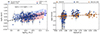 |
Fig. 4. Mass-size relation of late-type galaxies (left). The blue filled circles represents the data (of Sharma et al. 2023, employed in this work), and black dashed line shows the best-fit (slope and offset marked on plot). The blue and red shaded areas represent the mass-size relation of van der Wel et al. (2014) at z = 0.75 and z = 2.25, respectively. Ionized gas velocity dispersion as a function of redshift (right). The blue filled circles and brown hexagons represent the Sharma et al. (2023) and Übler et al. (2019) data, respectively. The brown dashed line represents the best fit of Übler et al. (2019) work. We notice that 73 out of the 263 (27.7%) galaxies from the Sharma et al. (2023) sample are common in the two datasets. |
Evolution of the velocity dispersion. The velocity dispersion of a galaxy is tightly coupled to its dynamical state and serves as an effective measure of turbulence. Its cosmic evolution can provide critical insights into the efficiency and nature of the underlying driving mechanisms, such as the baryonic feedback processes and gravitational interactions (e.g., Förster Schreiber et al. 2006; Genzel et al. 2011; Swinbank et al. 2012a; Newman et al. 2013; Wisnioski et al. 2015; Turner et al. 2017; Johnson et al. 2018; Übler et al. 2019, and references therein). Moreover, variations in the velocity dispersion with redshift could potentially suggest how galaxies interact with their environments, particularly the cosmic web (Glazebrook 2013). The correlation between the ionized gas velocity dispersion and redshift is a well-established phenomenon, as reviewed comprehensively by Glazebrook (2013) and Förster Schreiber & Wuyts (2020). In the right panel of Fig. 4, we show this relation for our sample and compared with those of Übler et al. (2019). We infer that both datasets are in fair agreement across all redshifts with similar intrinsic scatter (≈0.2 dex). The slight offset in this relation can be attributed to the difference in the kinematic modeling techniques used in our analysis.
3. Tully-Fisher relation
We assume that the galaxy masses (baryonic: stars and gas) scale with the circular velocities as a power-law with slope (α) and intercept (β), which can mathematically be defined as:

where, Y is the list of stellar (or baryonic) masses and X corresponds to the circular velocities (Vc). To obtain the best-fit to the data, we sample the likelihood using Markov Chain Monte Carlo (MCMC), which uses an orthogonal likelihood, defined as:
where, xi and yi denote the stellar mass and circular velocity lists, respectively, while σxi and σyi represent their associated errors. The parameter ζint refers to the intrinsic scatter in the direction orthogonal to the best-fit line, and σi gives the total scatter in the relation. We adopted this orthogonal likelihood fitting technique due to the significant scatter observed in high-redshift galaxies (∼0.25 dex) in both the stellar mass (at fixed velocity) and circular velocity (at fixed stellar mass). This scatter results in a dispersed relation, which is more accurately constrained by minimizing the scatter orthogonally along the best-fit line. This approach contrasts with the case of local disk galaxies, which exhibit a remarkably tight correlation in the Mstar − Vc (or Mbar − VC) plane with a scatter of approximately 0.026 − 0.1 dex on both the axes. In such cases, employing a vertical likelihood method (as described in Eq. (A.1)) is more appropriate, as demonstrated by Lelli et al. (2019). Further justification for the choice of orthogonal likelihood over vertical likelihood in the context of high-redshift data is provided in Appendix A. Additionally, we remark that when fitting the STFR and BTFR, we utilized the circular velocities calculated at Rout. As a result, the stellar and baryonic masses used in these fits are also constrained within the Rout region, and denoted as Mstar and Mbar. However, wherever we use the total stellar or baryonic masses, they are denoted as  or
or  . For detailed discussion on the choice of global and constrained masses, we refer to Appendix B.
In Fig. 5, we present the orthogonal likelihood fits for the STFR and BTFR (left and right panels, respectively). For the STFR, we obtained a slope of α = 3.03 ± 0.25, an offset of β = 3.34 ± 0.53, and an intrinsic scatter of ζint = 0.08 dex. Correspondingly, the BTFR yielded α = 3.21 ± 0.28, β = 3.16 ± 0.61, and ζint = 0.09 dex. These results are compared with previous studies, including both local and high-redshift studies of STFR and BTFR. For the STFR, we reference works by Reyes et al. (2011, z ≈ 0), Lapi et al. (2018, z ≈ 0), Di Teodoro et al. (2016, z ∼ 1), Übler et al. (2017, 0.9 ≤ z ≤ 2.3), Tiley et al. (2019, z ∼ 1), Pelliccia et al. (2017, z ∼ 0.9), Abril-Melgarejo et al. (2021, z ∼ 0.5 − 0.8) and Straatman et al. (2017, z ∼ 2 − 2.5). For the BTFR, we consider studies of Papastergis et al. (2016, z ≈ 0), Lelli et al. (2019, z ≈ 0), Übler et al. (2017, 0.9 ≤ z ≤ 2.3), Goddy et al. (2023, z ≈ 0), Abril-Melgarejo et al. (2021, z ∼ 0.5 − 0.8), Zaritsky et al. (2014, z ∼ 0), and Catinella et al. (2023, z ∼ 0). As evident from Fig. 5, although previous studies of STFR and BTFR, both local and at high redshifts, align well within 3σ uncertainties, the new data from Sharma et al. (2023) offers evidence of a marginal evolution in both the slope and zero-point of these relations. Specifically, we report a slightly shallower slope and an increase in the STFR zero-point compared to most previous studies, as reported in Table 1.
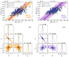 |
Fig. 5. Stellar and baryonic Tully-Fisher relations (STFR and BTFR), presented in the top-left and top-right panels, respectively. The blue-filled circles represent the data from Sharma et al. (2023), with gray error bars denoting uncertainties on each measurements. The solid orange and purple lines shows the best-fit curves obtained in this study using orthogonal likelihood, accompanied by the shaded regions representing the 3σ intrinsic scatter for the STFR and BTFR, respectively. The bottom-right corner of each plot displays the best-fit parameters. Additionally, the blue lines correspond to comparisons with local studies, while red lines represent the high-redshift data, as indicated in the upper left legend of each plot. The lower panel shows the posterior distributions (corner plots) resulting from the MCMC fitting process for the STFR and BTFR, shown in the left and right plots, respectively. The contours within these corner plots illustrate the 68%, 90%, and 99% credible intervals. For reference, we also show vertical likelihood fits of STFR and BTFR in Fig. D.1, which shows a huge difference in the slope and zero-point of the relation with respect to orthogonal likelihood. We report a difference of a factor of about 2. |
The slopes of STFR and BTFR obtained in this work along with a comparison to previous studies.
Initially, we assumed that the observed change in the slope might be solely attributable to the fitting technique. To understand this, we fitted our data using the slope and zero-point values reported in the previous studies (listed in Table 1) and calculated the intrinsic scatter around these reference lines. In Fig. 6, we show the orthogonal intrinsic scatter as a function of the slopes obtained from prior studies, for both STFR (in orange) and BTFR (in purple). Our analyses indicates consistency with the slope and intrinsic scatter observed in previous studies. However, notably, our fitting technique yields shallower slope and a reduced intrinsic scatter compared to previous studies, (see also Table 1).
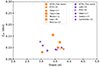 |
Fig. 6. Comparison of slopes and intrinsic scatters: we take the best-fits of previous studies as a face-value (x-axis) and apply them on our dataset to compute the orthogonal intrinsic scatter (y-axis) around the adopted best-fit lines. STFR studies are represented by orange markers, BTFR studies by purple, with each marker corresponding to a distinct study listed in the legends. |
Although, previous studies have reported similar results, we place greater trust in our measurements. The reason is the outcome of a comparative analysis of orthogonal and vertical likelihood fitting techniques, as detailed in Appendix A. In our study, we modeled the mock STFR data with high-z errors on individual measurements and scatter, akin to observations at high redshifts. We observed that the vertical likelihood method could not retrieve the true slope at high redshift, whereas the orthogonal likelihood method performed exceptionally well. We noted that the slope of the vertical likelihood differs by a factor of 1.5 ± 1 compared to the orthogonal likelihood. Upon comparing our best-fit STFR/BTFR slopes with those of previous studies that minimize vertical scatter (e.g., Reyes et al. 2011; Übler et al. 2017), we found a difference of factor ∼1.2 to 1.5, similar to the one we just stated. Therefore, we suggest that orthogonal likelihood fitting techniques work best for high-z datasets, which are prone to large scatter. Finally, we also fit the STFR and BTFR using Vmax, and observed that the slope only varies by about ±0.15 dex, which falls within the uncertainty range of the slope and zero-point provided using Vc. Based on these findings, we suggest that both the slope and the zero-point of the Tully-Fisher relation evolve modestly over cosmic time. Moreover, we learned that the slope, zero-point, and intrinsic scatter are all very sensitive to the preferred fitting technique.
As suggested in GS23, any changes in the systematic uncertainties in M*, SFR, or the intrinsic scatter in the gas scaling relation will increase the errors in the individual measurements of baryonic mass by about 0.2 dex. However, the slope of the BTFR remains consistent, varying by no more than 0.01 dex, which is within the reported uncertainty on the slope. We would also like to note that in this study, we do not focus on the evolution of the zero-point. This decision is based on our understanding that at high redshifts (z), the GS23 sample lacks low-mass galaxies due to Tolman surface brightness dimming (for further details, refer to Sharma et al. 2023), which are crucial for accurately constraining the zero-point of the TFR.
Furthermore, we explored the STFR and BTFR relations within different redshift bins, as shown in the left and right panels of Fig. 7, respectively. In particular, we divided our galaxies into two redshift bins: 0.6 ≤ z ≤ 1.2 ( ) and 1.2 < z ≤ 2.3 (
 ), fitting each bin independently using the aforementioned technique. Although Fig. 7 displays the best-fit results for both redshift bins, it is important to note that the z ∼ 1.5 bin is biased toward massive galaxies and does not encompass the typical mass (log(Mstar/bar [M⊙]) = 9.0 − 11.5) and circular velocity (log(Vc km/s) = 1.6 − 2.85) ranges upon which the fundamental TFR is established. Therefore, the results of the STFR and BTFR relations of z ∼ 1.5 bin are not representative (or pertinent); hence, we do not draw any conclusions for this redshift bin. Conversely, the STFR and BTFR relations at z ∼ 1 cover typical mass and velocity range, and the fitting results are very similar to the one those derived from the full dataset. To be precise, for STFR, we find α = 3.13, β = 3.20, and ζint = 0.07 dex, while for BTFR, we have α = 3.35, β = 2.89, and ζint = 0.08 dex. Thus, even when we restrict our analysis to galaxies at z ∼ 1, we discern a nominal evolution in the slope and zero-point (β/α) of the TFR relation at high redshifts.
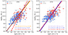 |
Fig. 7. STFR and BTFR, respectively, separated into two redshift bins: 0.6 ≤ z ≤ 1.2 ( |


4. Discussion
To reaffirm the validity of the GS23 dataset, which is a fair representative of the main sequence of star-forming galaxies as shown in Fig. 1, we further demonstrate its ability to accurately represent fundamental relations previously explored within similar redshift ranges using high-resolution photometry and resolved kinematics. Specifically, the mass-size relation (van der Wel et al. 2014) and cosmic evolution of the velocity dispersion (Übler et al. 2019) are shown in the left and right panels of Fig. 4, respectively. It is evident from these figures that the dataset studied in Sharma et al. (2023) is fairly representing these fundamental scaling relations, thereby reinforcing the robustness of GS23 data and its suitability in studying the TFR.
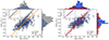 |
Fig. 8. Comparison of STFR and BTFR with local studies. Left Panel: STFR comparison between the GS23 dataset (blue filled circles) and Lapi2018 (gray open circles). The best fit for Lapi2018 is represented by the black solid line, while the best-fit of this work (on GS23 data) is shown in orange. Right Panel: BTFR comparison between the GS23 dataset (blue filled circles) and Lelli2019 (brown open circles). The best fit for Lelli2019 is indicated by the brown solid line, while the best-fit of this work in purple. In both panels, the inset provides a zoomed-in view of the local and high-z fits within the range 9.0 ≤ log(Mstar/bar [M⊙]) ≤ 11.5 and 1.65 ≤ log(Vc [km/s]) ≤ 2.75. Additionally, for dataset comparison, histograms of the x and y axes are included: Lapi2018 in gray, Lelli2019 in brown and GS23 in blue. In both the STFR and BTFR cases, we observe a divergent evolution in the slope, while the zero-point remains uncertain due to the absence of low-mass galaxies at high redshifts. |
Moreover, the GS23 dataset spans stellar mass and circular velocity range as explored in local STFR studies. In particular, circular velocities range between 1.6 ≲ log(Vc [km/s]) ≲ 2.85 and stellar masses 8.89 ≲ log(Mstar [M⊙]) ≲ 11.5, which is the same range as explored in Reyes et al. (2011) and Lapi et al. (2018). Therefore, our sample is relatively free of selection bias (in terms of mass and velocity range), hence, it allows us to study the STFR, as well as BTFR, as shown in Fig. 5 left and right panels, respectively. We report a marginal evolution in the slope and zero-point of the STFR and BTFR relations for z ≤ 1; whereas at z ∼ 1.5, we do not draw conclusions on the evolution of the slope or zero-point due to insufficient data in the lower mass and velocity end. In subsequent sections, we discuss our results in light of previous local and high-redshift studies.
4.1. Comparison with local studies
To compare the STFR, we utilized the data from Lapi et al. (2018, hereafter Lapi2018) as a benchmark. In the left panel of Fig. 8, we juxtapose the dataset of Lapi2018 with GS23. While the velocity ranges of both datasets overlap significantly, we observe that at higher velocities, local galaxies are more massive compared to their high-redshift counterparts. In other words, at fixed stellar masses (bench-marking against local galaxies), high-redshift galaxies exhibit fast rotation, a phenomenon also reported in previous studies (e.g., Puech et al. 2008, 2010; Cresci et al. 2009; Gnerucci et al. 2011; Swinbank et al. 2012b; Price et al. 2016; Tiley et al. 2016; Straatman et al. 2017; Übler et al. 2017; Rizzo et al. 2020; Lelli 2022; Lelli et al. 2023; Sharma et al. 2023). In particular, the slope and zero-point of the high-redshift STFR deviate from their standard values (e.g., Lapi et al. 2018) by approximately a factor of 1.2 and 0.72, respectively. Specifically, in the redshift range 0.6 ≤ z ≤ 2.5, we obtain a slope of α = 3.03 ± 0.25 and an offset of β = 3.34 ± 0.53. Thus, we report a divergent evolution in the STFR over cosmic time. This marginal evolution is most-likely due the evolutionary stages of galaxies, which we plan to investigate in future work using cosmological simulations.
To compare the BTFR relation, we utilize the dataset from Lelli et al. (2019, hereafter Lelli2019) and juxtapose their data in the right panel of Fig. 8. Although GS23 dataset overlap seamlessly with Lelli2019, we notice that our dataset does not encompass galaxies with lower baryonic masses (Mbar < 109.35M⊙) and lower velocities (Vc < 40km/s) as observed in local galaxies. This absence could be attributed to the Tolman dimming effect (Tolman 1930; Pahre et al. 1996), as suggested in GS23. Due to these missing galaxies in the lower mass and velocity range, we refrain from making definitive conclusions regarding the zero-point of the BTFR at high redshifts. Secondly, similar to the STFR, at fixed baryonic mass, galaxies at high redshifts seems to rotate faster. Consequently, we observe a slightly shallower slope at high redshifts, with respect to local approaches.
4.2. Comparison with high-z studies
We acknowledge that Übler et al. (2017, hereafter U17) and Tiley et al. (2019, hereafter AT19) pioneered the study of the TFR at high redshifts, using large-datasets of IFU surveys: KMOS3D and KROSS surveys, respectively. Although, GS23 dataset consists of a sub-sample from both the KMOS3D and KROSS surveys, there exists discrepancies between the STFR and BTFR fits of U17, AT19, and this work. To understand these discrepancies, we present a comparative analysis of the STFR and BTFR datasets in Figs. 9 and 10, respectively. Moreover, we provide a detailed tailored comparison in Appendix C. We remark that AT19 only study the STFR, while U17 studies both STFR and BTFR.
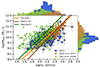 |
Fig. 9. Comparison of STFR data of this work with datasets of other high-redshift studies: Tiley et al. (2019, green squares) and Übler et al. (2017, brown hexagons). The orange, green, and brown lines represent the best-fit results for our study, Tiley et al. (2019), and Übler et al. (2017), respectively. To facilitate a comprehensive comparison of the datasets, we provide histograms showing the distributions of stellar mass and circular velocities, both horizontally and vertically, color-coded same as their respective datasets. We note that the velocities for Tiley et al. (2019) are rotational velocities and not circular velocities. |
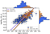 |
Fig. 10. Comparison of BTFR dataset of this study with Übler et al. (2017, brown hexagons). The purple and brown lines represent the best-fit results for our study and Übler et al. (2017), respectively. For a comprehensive comparison of the datasets, we provide histograms showing the distributions of stellar mass and circular velocities, both horizontally and vertically, color-coded according to their respective datasets. |
First, we note that the kinematic modeling techniques employed by the three studies are distinct. Differently to the approaches in A19 and U17 (see details in respective studies or briefly in Appendix C), GS23 fit the kinematics in 3D space. Some previous studies have shown that the 3D forward modeling allows for more accurate estimates of observed rotation velocities compared to 2D methods (Di Teodoro et al. 2016; Sharma et al. 2021, 2023). In particular, the 2D kinematic modeling techniques overestimate the velocity dispersion and provide underestimated rotation velocities. Consequently, the discrepancies between these studies are expected. However, other factors that may contribute to these discrepancies are discussed below for each study separately.
AT19. Rotation curves are derived along the major axis of the 2D velocity map, and beam-smearing corrections are applied only at the outer radius (2 − 5RD). Moreover, the rotation curves were not corrected for the pressure gradients. Consequently, we anticipate lower circular velocity estimates in comparison to GS23. This is indeed evident in Fig. 9. The median value of the circular velocity distribution in the AT19 dataset is ≈100 km/s, whereas it is ≈150 km/s in GS23, despite clear overlap of stellar mass distributions. Additionally, upon implementing the sample selection criteria (Vc/σ > 3) used in AT19 and utilizing rotation velocities (without pressure corrections), as illustrated in Fig. C.1, we still evident discrepancies in both the distributions and the best-fit results. Moreover, as shown in Fig. 6, when we applied the AT19 best-fit to the GS23 dataset, we observe an intrinsic scatter of 0.16 dex, which is a factor of 2 higher than our estimates. Therefore, the AT19 fit is not applicable to the GS23 dataset. Finally, we suggest that the observed differences between the best fits of AT19 and GS23 are primarily due to discrepant kinematic modeling methods and variations in fitting techniques.
U17. Rotation curves are derived from the 2D velocity maps accounting for beam smearing and pressure gradient corrections. However, their pressure gradient corrections are applied under the assumption of constant and isotropic velocity dispersions. In Sharma et al. (2021) and Kretschmer et al. (2021), it is shown that the assumption of constant and isotropic velocity dispersion leads to overestimated circular velocities, when corrected for pressure gradients, especially, in low rotation to dispersion ratio galaxies (v/σ ≲ 1.5). Hence, circular velocity estimates of U17 are expected to be higher than GS23 estimates. It is indeed evident in Figs. 9, 10, and C.2. Even when we apply the sample selection cut ( ) used in U17, we still observe high circular velocities at fixed stellar mass, as shown in Fig. C.2. In particular, we notice that U17 objects are biased toward higher velocities (
 ) and stellar and baryonic masses (
 /
/  ). While, GS23 dataset covers a typical mass and velocity ranges, we suggest that this is most-likely the primary reason for the discrepant STFR and BTFR fits in U17 with respect to our work. Furthermore, when we apply the U17 best-fit to the GS23 dataset, we observe an intrinsic scatter of ∼0.1 dex, which is a factor of 1.25 higher than our estimates. This suggest that discrepancies are also induced due to fitting techniques.
4.3. Comparison of fitting techniques
In this work, we performed a mock analysis of orthogonal and vertical likelihood fitting techniques on the stellar Tully-Fisher relation, as discussed in Sect. 3 and detailed in Appendix A. The mock analysis results are shown in Figs. A.1 and A.2. We observe that the vertical likelihood fitting technique works well for the Local Universe, where the intrinsic scatter is of the order of 0.01–0.1 dex. However, it underestimates the slope when intrinsic scatter exceeds 0.1 dex, as observed in the high-redshift data. In contrast, the orthogonal likelihood fitting technique performs best in both cases. Notably, it retrieves the correct slope with a precision error of less than ±0.02 dex. Consequently, we employed the orthogonal likelihood fitting technique in our work. The results of high-redshift STFR and BTFR fits obtained using orthogonal and vertical likelihood methods are presented in Figs. 5 and D.1, respectively. Interestingly, the slopes obtained using the vertical likelihood for the STFR and BTFR differ from the orthogonal method’s best fits by 1.72 dex and 1.98 dex, respectively. Therefore, we recommend using the orthogonal likelihood fitting technique for STFR and BTFR studies – or any scaling relations where data is subject to large uncertainties. For the reference, we have made our code publicly available via a GitHub repository2.
5. Conclusions
In this study, we investigate the stellar and baryonic Tully-Fisher relations over a broad redshift range of 0.6 ≤ z ≤ 2.5 using data from Sharma et al. (2023). To effectively address the substantial scatter prevalent among high-redshift galaxies, as elaborated in Appendix A. We employed an orthogonal likelihood fitting technique, which minimizes the intrinsic scatter orthogonal to the best-fit line. The outcomes of our fitting methodology are presented in Fig. 5. For the STFR, our analysis yielded a slope of α = 3.03 ± 0.25, an intercept β = 3.34 ± 0.53, and an intrinsic scatter of ζint = 0.08 dex. Correspondingly, the best-fit BTFR parameters are: α = 3.21 ± 0.28, β = 3.16 ± 0.61, and ζint = 0.09 dex. That is, the slopes of the STFR and BTFR are slower by a factor of ∼1.23 and ∼1.15, respectively, compared to those observed in the Local Universe.
We also explored the relations for different redshift bins and found that the z ∼ 1.5 bin was biased toward massive galaxies and hence inconclusive. Conversely, the z ∼ 1 bin, devoid of such a bias, yielded results within the agreement to those derived from the complete (full) dataset, and affirmed the presence of minimal evolution in both the STFR and BTFR. When comparing our findings with local studies, we observed slight deviations, as shown in Fig. 8. Moreover, a comparison with previous high-redshift studies highlight differences due to kinematic modeling methods, fitting techniques, and sample selection (see Sect. 4.2 and Appendix C).
Through a comparative analysis of the outcomes obtained using orthogonal and vertical likelihood fitting methods, we have discerned a significant impact of fitting techniques on determining the slope and zero-point of scaling relations. Specifically, employing the vertical likelihood fitting technique at high redshifts (outlined in Appendix A) led to a shallower slope of the STFR/BTFR by a factor of ∼2.5, along with a correspondingly higher zero-point, as shown in Fig. D.1. This discrepancy arises from the inherent scatter within the observed data. Therefore, before picking a specific fitting technique, we suggest conducting mock data analyses (including observed scatter) to evaluate the performance of different fitting techniques on given observations, as we demonstrate in Appendix A.
Based on our findings, we conclude that the Tully-Fisher relation (TFR) exhibits a subtle shift in both the slope and zero-point values across cosmic time. This variation is most-likely due to dominant mechanisms driving galaxy evolution, such as gas accretion, star formation, mergers, or baryonic feedback. Therefore, we propose that the TFR is an empirical relation, rather than a fundamental one in galaxy evolution, as it seems to show a dependency on galaxy’s physical condition at a given epoch. Therefore, we emphasize the importance of studying the TFR across cosmic time using cosmological galaxy simulations to gain deeper insights into the underlying physical processes shaping the galaxy properties and its evolution across cosmic scales.
For an exponential thin disk, the stellar-disk radius is defined as RD = 0.59 Re. Under the same assumption, the scale length that encloses 80% of the stellar mass is referred to as the optical radius and defined as Ropt = 3.2 RD. For more comprehensive details, we refer to Persic et al. (1996).
Acknowledgments
We thank the anonymous referee for constructive feedback. GS acknowledges the SARAO postdoctoral fellowship (UID No.: 97882) and the support provided by the University of Strasbourg Institute for Advanced Study (USIAS) within the French national programme Investment for the Future (Excellence Initiative) IdEx-Unistra. GS also thanks IIT Hyderabad for funding the January 2024 collaboration visit, which has led to this publication.
References
- Abril-Melgarejo, V., Epinat, B., Mercier, W., et al. 2021, A&A, 647, A152 [NASA ADS] [CrossRef] [EDP Sciences] [Google Scholar]
- Arnouts, S., Cristiani, S., Moscardini, L., et al. 1999, MNRAS, 310, 540 [Google Scholar]
- Avila-Reese, V., Zavala, J., Firmani, C., & Hernández-Toledo, H. M. 2008, AJ, 136, 1340 [CrossRef] [Google Scholar]
- Barden, M., Rix, H.-W., Somerville, R. S., et al. 2005, ApJ, 635, 959 [NASA ADS] [CrossRef] [Google Scholar]
- Bell, E. F., & de Jong, R. S. 2001, ApJ, 550, 212 [Google Scholar]
- Blumenthal, G. R., Faber, S., Primack, J. R., & Rees, M. J. 1984, Nature, 311, 517 [NASA ADS] [CrossRef] [Google Scholar]
- Böhm, A., Ziegler, B. L., Saglia, R. P., et al. 2004, A&A, 420, 97 [EDP Sciences] [Google Scholar]
- Boselli, A., Lequeux, J., & Gavazzi, G. 2002, A&A, 384, 33 [NASA ADS] [CrossRef] [EDP Sciences] [Google Scholar]
- Burkert, A., Genzel, R., Bouché, N., et al. 2010, ApJ, 725, 2324 [Google Scholar]
- Burkert, A., Schreiber, N. F., Genzel, R., et al. 2016, ApJ, 826, 214 [CrossRef] [Google Scholar]
- Carollo, C. M., Bschorr, T. J., Renzini, A., et al. 2013, ApJ, 773, 112 [NASA ADS] [CrossRef] [Google Scholar]
- Catinella, B., Cortese, L., Tiley, A. L., et al. 2023, MNRAS, 519, 1098 [Google Scholar]
- Chowdhury, A., Kanekar, N., & Chengalur, J. N. 2022, ApJ, 941, L6 [NASA ADS] [CrossRef] [Google Scholar]
- Conselice, C. J., Bundy, K., Ellis, R. S., et al. 2005, ApJ, 628, 160 [Google Scholar]
- Courteau, S. 1997, AJ, 114, 2402 [Google Scholar]
- Cresci, G., Hicks, E. K. S., Genzel, R., et al. 2009, ApJ, 697, 115 [Google Scholar]
- Daddi, E., Renzini, A., Pirzkal, N., et al. 2005, ApJ, 626, 680 [NASA ADS] [CrossRef] [Google Scholar]
- Daddi, E., Elbaz, D., Walter, F., et al. 2010, ApJ, 714, L118 [NASA ADS] [CrossRef] [Google Scholar]
- Davies, R. I., Maciejewski, W., Hicks, E. K. S., et al. 2009, ApJ, 702, 114 [NASA ADS] [CrossRef] [Google Scholar]
- Davies, R., Förster Schreiber, N. M., Cresci, G., et al. 2011, ApJ, 741, 69 [NASA ADS] [CrossRef] [Google Scholar]
- de Blok, W. J. G., Walter, F., Brinks, E., et al. 2008, AJ, 136, 2648 [NASA ADS] [CrossRef] [Google Scholar]
- Di Teodoro, E., Fraternali, F., & Miller, S. 2016, A&A, 594, A77 [NASA ADS] [CrossRef] [EDP Sciences] [Google Scholar]
- Feast, M. W. 1994, MNRAS, 266, 255 [NASA ADS] [CrossRef] [Google Scholar]
- Ferrarese, L., Ford, H. C., Huchra, J., et al. 2000, ApJS, 128, 431 [Google Scholar]
- Foreman, S., & Scott, D. 2012, Phys. Rev. Lett., 108, 141302 [NASA ADS] [CrossRef] [Google Scholar]
- Foreman-Mackey, D., Hogg, D. W., Lang, D., & Goodman, J. 2013, PASP, 125, 306 [Google Scholar]
- Förster Schreiber, N. M., Genzel, R., Lehnert, M. D., et al. 2006, ApJ, 645, 1062 [Google Scholar]
- Freedman, W. L., Madore, B. F., Scowcroft, V., et al. 2011, AJ, 142, 192 [CrossRef] [Google Scholar]
- Freundlich, J., Combes, F., Tacconi, L. J., et al. 2019, A&A, 622, A105 [NASA ADS] [CrossRef] [EDP Sciences] [Google Scholar]
- Förster Schreiber, N. M., & Wuyts, S. 2020, ARA&A, 58, 661 [Google Scholar]
- Gavazzi, G., Fumagalli, M., Cucciati, O., & Boselli, A. 2010, A&A, 517, A73 [NASA ADS] [CrossRef] [EDP Sciences] [Google Scholar]
- Genzel, R., Newman, S., Jones, T., et al. 2011, ApJ, 733, 101 [Google Scholar]
- Genzel, R., Tacconi, L. J., Lutz, D., et al. 2015, ApJ, 800, 20 [Google Scholar]
- Genzel, R., Schreiber, N. F., Ubler, H., et al. 2017, Nature, 543, 397 [NASA ADS] [CrossRef] [Google Scholar]
- Giovanelli, R., Haynes, M. P., da Costa, L. N., et al. 1997a, ApJ, 477, L1 [CrossRef] [Google Scholar]
- Giovanelli, R., Haynes, M. P., Herter, T., et al. 1997b, AJ, 113, 53 [NASA ADS] [CrossRef] [Google Scholar]
- Girardi, M., Manzato, P., Mezzetti, M., Giuricin, G., & Limboz, F. 2002, ApJ, 569, 720 [NASA ADS] [CrossRef] [Google Scholar]
- Glazebrook, K. 2013, PASA, 30, e056 [NASA ADS] [CrossRef] [Google Scholar]
- Gnerucci, A., Marconi, A., Cresci, G., et al. 2011, A&A, 528, A88 [NASA ADS] [CrossRef] [EDP Sciences] [Google Scholar]
- Goddy, J. S., Stark, D. V., Masters, K. L., et al. 2023, MNRAS, 520, 3895 [NASA ADS] [CrossRef] [Google Scholar]
- Gurovich, S., Freeman, K., Jerjen, H., Staveley-Smith, L., & Puerari, I. 2010, AJ, 140, 663 [NASA ADS] [CrossRef] [Google Scholar]
- Harrison, C. M., Johnson, H. L., Swinbank, A. M., et al. 2017, MNRAS, 467, 1965 [Google Scholar]
- Ilbert, O., Arnouts, S., McCracken, H. J., et al. 2006, A&A, 457, 841 [NASA ADS] [CrossRef] [EDP Sciences] [Google Scholar]
- Johnson, H. L., Harrison, C. M., Swinbank, A. M., et al. 2018, MNRAS, 474, 5076 [NASA ADS] [CrossRef] [Google Scholar]
- Karachentsev, I. D., Mitronova, S. N., Karachentseva, V. E., Kudrya, Y. N., & Jarrett, T. H. 2002, A&A, 396, 431 [NASA ADS] [CrossRef] [EDP Sciences] [Google Scholar]
- Kassin, S. A., Weiner, B. J., Faber, S. M., et al. 2007, ApJ, 660, L35 [Google Scholar]
- Keres, D., Yun, M. S., & Young, J. S. 2003, ApJ, 582, 659 [NASA ADS] [CrossRef] [Google Scholar]
- Kretschmer, M., Dekel, A., Freundlich, J., et al. 2021, MNRAS, 503, 5238 [NASA ADS] [CrossRef] [Google Scholar]
- Krishak, A., & Desai, S. 2022, Open J. Astrophys., 5, 9 [NASA ADS] [CrossRef] [Google Scholar]
- Lagos, C. D. P., Baugh, C. M., Lacey, C. G., et al. 2011, MNRAS, 418, 1649 [CrossRef] [Google Scholar]
- Lagos, C. D. P., Theuns, T., Stevens, A. R. H., et al. 2017, MNRAS, 464, 3850 [NASA ADS] [CrossRef] [Google Scholar]
- Lapi, A., Salucci, P., & Danese, L. 2018, ApJ, 859, 2 [Google Scholar]
- Lelli, F. 2022, in Inward bound: bulges from high redshifts to the Milky Way. Online Workshop held 2-6 May, 3 [Google Scholar]
- Lelli, F., McGaugh, S. S., & Schombert, J. M. 2016, ApJ, 816, L14 [Google Scholar]
- Lelli, F., McGaugh, S. S., Schombert, J. M., Desmond, H., & Katz, H. 2019, MNRAS, 484, 3267 [NASA ADS] [CrossRef] [Google Scholar]
- Lelli, F., Zhang, Z.-Y., Bisbas, T. G., et al. 2023, A&A, 672, A106 [NASA ADS] [CrossRef] [EDP Sciences] [Google Scholar]
- Madau, P., & Dickinson, M. 2014, ARA&A, 52, 415 [Google Scholar]
- Mao, S., Mo, H. J., & White, S. D. M. 1998, MNRAS, 297, L71 [Google Scholar]
- Martin, A. M., Papastergis, E., Giovanelli, R., et al. 2010, ApJ, 723, 1359 [NASA ADS] [CrossRef] [Google Scholar]
- Masters, K. L., Springob, C. M., Haynes, M. P., & Giovanelli, R. 2006, ApJ, 653, 861 [Google Scholar]
- Mathewson, D. S., Ford, V. L., & Buchhorn, M. 1992, ApJS, 81, 413 [NASA ADS] [CrossRef] [Google Scholar]
- McGaugh, S. S. 2005, Phys. Rev. Lett., 95, 171302 [NASA ADS] [CrossRef] [Google Scholar]
- McGaugh, S. S., & Schombert, J. M. 2015, ApJ, 802, 18 [NASA ADS] [CrossRef] [Google Scholar]
- McGaugh, S. S., Schombert, J. M., Bothun, G. D., & de Blok, W. J. G. 2000, ApJ, 533, L99 [Google Scholar]
- Mercier, W., Epinat, B., Contini, T., et al. 2022, A&A, 665, A54 [NASA ADS] [CrossRef] [EDP Sciences] [Google Scholar]
- Miller, S. H., Bundy, K., Sullivan, M., Ellis, R. S., & Treu, T. 2011, ApJ, 741, 115 [Google Scholar]
- Mo, H. J., & Mao, S. 2000, MNRAS, 318, 163 [NASA ADS] [CrossRef] [Google Scholar]
- Mosleh, M., Williams, R. J., Franx, M., & Kriek, M. 2011, ApJ, 727, 5 [NASA ADS] [CrossRef] [Google Scholar]
- Neill, J. D., Seibert, M., Tully, R. B., et al. 2014, ApJ, 792, 129 [CrossRef] [Google Scholar]
- Newman, S. F., Genzel, R., Förster Schreiber, N. M., et al. 2013, ApJ, 767, 104 [NASA ADS] [CrossRef] [Google Scholar]
- Noeske, K. G., Weiner, B. J., Faber, S. M., et al. 2007, ApJ, 660, L43 [CrossRef] [Google Scholar]
- Pahre, M. A., Djorgovski, S. G., & de Carvalho, R. R. 1996, ApJ, 456, L79 [NASA ADS] [CrossRef] [Google Scholar]
- Papastergis, E., Adams, E. A. K., & van der Hulst, J. M. 2016, A&A, 593, A39 [NASA ADS] [CrossRef] [EDP Sciences] [Google Scholar]
- Pelliccia, D., Tresse, L., Epinat, B., et al. 2017, A&A, 599, A25 [NASA ADS] [CrossRef] [EDP Sciences] [Google Scholar]
- Pérez-González, P. G., Rieke, G. H., Villar, V., et al. 2008, ApJ, 675, 234 [Google Scholar]
- Persic, M., Salucci, P., & Stel, F. 1996, MNRAS, 281, 27 [Google Scholar]
- Pizagno, J., Prada, F., Weinberg, D. H., et al. 2007, AJ, 134, 945 [Google Scholar]
- Price, S. H., Kriek, M., Shapley, A. E., et al. 2016, ApJ, 819, 80 [Google Scholar]
- Puech, M., Flores, H., Hammer, F., et al. 2008, A&A, 484, 173 [CrossRef] [EDP Sciences] [Google Scholar]
- Puech, M., Hammer, F., Flores, H., et al. 2010, A&A, 510, A68 [NASA ADS] [CrossRef] [EDP Sciences] [Google Scholar]
- Read, J., Iorio, G., Agertz, O., & Fraternali, F. 2016, MNRAS, 462, 3628 [NASA ADS] [CrossRef] [Google Scholar]
- Reyes, R., Mandelbaum, R., Gunn, J., Pizagno, J., & Lackner, C. 2011, MNRAS, 417, 2347 [CrossRef] [Google Scholar]
- Rizzo, F., Vegetti, S., Powell, D., et al. 2020, Nature, 584, 201 [Google Scholar]
- Rodighiero, G., Daddi, E., Baronchelli, I., et al. 2011, ApJ, 739, L40 [Google Scholar]
- Saracco, P., Longhetti, M., & Gargiulo, A. 2011, MNRAS, 412, 2707 [NASA ADS] [CrossRef] [Google Scholar]
- Sharma, G., Salucci, P., Harrison, C. M., van de Ven, G., & Lapi, A. 2021, MNRAS, 503, 1753 [CrossRef] [Google Scholar]
- Sharma, G., Freundlich, J., van de Ven, G., et al. 2023, A&A, submitted [arXiv:2309.04541] [Google Scholar]
- Shen, S., Mo, H. J., White, S. D. M., et al. 2003, MNRAS, 343, 978 [NASA ADS] [CrossRef] [Google Scholar]
- Sorce, J. G., Courtois, H. M., Tully, R. B., et al. 2013, ApJ, 765, 94 [Google Scholar]
- Speagle, J. S., Steinhardt, C. L., Capak, P. L., & Silverman, J. D. 2014, ApJS, 214, 15 [Google Scholar]
- Stark, D. V., McGaugh, S. S., & Swaters, R. A. 2009, AJ, 138, 392 [CrossRef] [Google Scholar]
- Steinmetz, M., & Navarro, J. F. 1999, ApJ, 513, 555 [CrossRef] [Google Scholar]
- Straatman, C. M. S., Glazebrook, K., Kacprzak, G. G., et al. 2017, ApJ, 839, 57 [Google Scholar]
- Swinbank, A. M., Smail, I., Sobral, D., et al. 2012a, ApJ, 760, 130 [NASA ADS] [CrossRef] [Google Scholar]
- Swinbank, A. M., Sobral, D., Smail, I., et al. 2012b, MNRAS, 426, 935 [NASA ADS] [CrossRef] [Google Scholar]
- Tacconi, L. J., Genzel, R., Saintonge, A., et al. 2018, ApJ, 853, 179 [Google Scholar]
- Tacconi, L. J., Genzel, R., & Sternberg, A. 2020, ARA&A, 58, 157 [NASA ADS] [CrossRef] [Google Scholar]
- Teodoro, E. D., & Fraternali, F. 2015, MNRAS, 451, 3021 [NASA ADS] [CrossRef] [Google Scholar]
- Tiley, A., Bureau, M., Cortese, L., et al. 2019, MNRAS, 482, 2166 [NASA ADS] [CrossRef] [Google Scholar]
- Tiley, A. L., Stott, J. P., Swinbank, A. M., et al. 2016, MNRAS, 460, 103 [Google Scholar]
- Tolman, R. C. 1930, Proc. Nat. Acad. Sci., 16, 511 [NASA ADS] [CrossRef] [Google Scholar]
- Toribio, M. C., Solanes, J. M., Giovanelli, R., Haynes, M. P., & Martin, A. M. 2011, ApJ, 732, 93 [NASA ADS] [CrossRef] [Google Scholar]
- Torres-Flores, S., Epinat, B., Amram, P., Plana, H., & Mendes de Oliveira, C. 2011, MNRAS, 416, 1936 [Google Scholar]
- Tully, R. B., & Fisher, J. R. 1977, A&A, 54, 661 [NASA ADS] [Google Scholar]
- Tully, R. B., & Pierce, M. J. 2000, ApJ, 533, 744 [NASA ADS] [CrossRef] [Google Scholar]
- Turner, O. J., Harrison, C. M., Cirasuolo, M., et al. 2017, Arxiv e-prints [arXiv:1711.03604] [Google Scholar]
- Übler, H., Förster Schreiber, N. M., Genzel, R., et al. 2017, ApJ, 842, 121 [Google Scholar]
- Übler, H., Genzel, R., Wisnioski, E., et al. 2019, ApJ, 880, 48 [Google Scholar]
- Valenzuela, O., Rhee, G., Klypin, A., et al. 2007, ApJ, 657, 773 [NASA ADS] [CrossRef] [Google Scholar]
- van der Wel, A., Holden, B. P., Zirm, A. W., et al. 2008, ApJ, 688, 48 [NASA ADS] [CrossRef] [Google Scholar]
- van der Wel, A., Franx, M., van Dokkum, P. G., et al. 2014, ApJ, 788, 28 [Google Scholar]
- van Starkenburg, L., van der Werf, P. P., Yan, L., & Moorwood, A. F. M. 2006, A&A, 450, 25 [NASA ADS] [CrossRef] [EDP Sciences] [Google Scholar]
- Vergani, D., Epinat, B., Contini, T., et al. 2012, A&A, 546, A118 [NASA ADS] [CrossRef] [EDP Sciences] [Google Scholar]
- Verheijen, M. A. W., & Sancisi, R. 2001, A&A, 370, 765 [NASA ADS] [CrossRef] [EDP Sciences] [Google Scholar]
- Weijmans, A.-M., Krajnović, D., Van De Ven, G., et al. 2008, MNRAS, 383, 1343 [NASA ADS] [CrossRef] [Google Scholar]
- Wellons, S., Faucher-Giguère, C.-A., Anglés-Alcázar, D., et al. 2020, MNRAS, 497, 4051 [NASA ADS] [CrossRef] [Google Scholar]
- Whitaker, K. E., van Dokkum, P. G., Brammer, G., & Franx, M. 2012, ApJ, 754, L29 [Google Scholar]
- Williams, M. J., Bureau, M., & Cappellari, M. 2010, MNRAS, 409, 1330 [Google Scholar]
- Wisnioski, E., Förster Schreiber, N. M., Wuyts, S., et al. 2015, ApJ, 799, 209 [Google Scholar]
- Wisnioski, E., Förster Schreiber, N. M., Fossati, M., et al. 2019, ApJ, 886, 124 [Google Scholar]
- Wuyts, S., Förster Schreiber, N. M., van der Wel, A., et al. 2011, ApJ, 742, 96 [NASA ADS] [CrossRef] [Google Scholar]
- Wuyts, S., Förster Schreiber, N. M., Wisnioski, E., et al. 2016, ApJ, 831, 149 [Google Scholar]
- Zaritsky, D., Courtois, H., Muñoz-Mateos, J.-C., et al. 2014, AJ, 147, 134 [CrossRef] [Google Scholar]
- Ziegler, B. L., Böhm, A., Fricke, K. J., et al. 2002, ApJ, 564, L69 [Google Scholar]
- Zwaan, M. A., Meyer, M. J., Staveley-Smith, L., & Webster, R. L. 2005, MNRAS, 359, L30 [NASA ADS] [CrossRef] [Google Scholar]
Appendix A: Fitting techniques
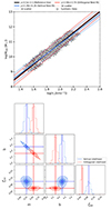 |
Fig. A.1. Vertical and orthogonal likelihood fitting on mock data resembling the local stellar and baryonic Tully-Fisher datasets. Upper Panel: Mock dataset depicted as open black circles with errors, accompanied by the best-fit lines. The solid black line represents the true slope of 3.5 used for generating the mock data. The blue and red solid lines correspond to the best fits obtained using the vertical and orthogonal likelihood methods, respectively. Both best-fit lines are followed by 3σ intrinsic scatter regions, indicated with the same color code as the best fits. Lower Panel: Posterior distributions resulting from MCMC-fitting for the vertical and orthogonal likelihoods are shown in blue and red, respectively. The contours within these corner plots illustrates the 68%, 90%, and 99% credible intervals. |
In this section we discuss the fitting techniques used in estimating the slopes and intercepts. We use the MCMC sampler emcee (Foreman-Mackey et al. 2013) to estimate the best-fit parameters. In our work, we fit a linear model y = αx + β to a set of N datapoints (xi, yi) with errors (σxi, σyi). We mainly consider two possible likelihoods for the parameter estimation. The first is a vertical likelihood that considers intrinsic scatter in the vertical direction, i.e., the intrinsic scatter varies only along the y-direction and not the x-direction (Reyes et al. 2011; Lelli et al. 2019). The second considers the intrinsic scatter to be orthogonal to the best-fit line (Papastergis et al. 2016). The vertical log-likelihood function follows:
whereas, the orthogonal log-likelihood function is defined as:
In Equation (A.2) and (A.4), σi encapsulate the expressions for the total scatter in each case, calculated by taking into account the individual errors on the data points (σxi, σyi) along with the intrinsic scatter ζint.
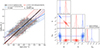 |
Fig. A.2. Vertical and orthogonal likelihood fitting on mock data resembling the high-redshift stellar and baryonic Tully-Fisher relations. Left Panel: Mock dataset depicted as open black circles with associated errors, accompanied by the best-fit lines. The solid black line represents the true slope of 3.5 used for generating the mock data. The blue and red solid lines correspond to the best fits obtained using the vertical and orthogonal likelihood methods, respectively. Both best-fit lines are followed by 3σ intrinsic scatter regions, indicated with the same color code as the best fits. Right Panel: Posterior distributions resulting from the MCMC fitting process for the vertical and orthogonal likelihoods are shown in blue and red, respectively. The contours within these corner plots illustrates the 68%, 90%, and 99% credible intervals. |
As it is not immediately evident which method is more suitable for our purposes, we use synthetic data to test the efficacy of both the methods by determining which of these likelihoods can recover the correct regression relation. First, we generate mock data using the commonly accepted value of the STFR, α = 3.5, and error values in the range of 0.12-0.15 and 0.03-0.08 for the yi (stellar mass) and xi (circular velocity) variables generated using a uniform distribution. The scatter (spread) in the data-points is taken to be about 0.1 dex, which is an average value obtained from previous studies (Reyes et al. 2011; Lapi et al. 2018; Lelli et al. 2019). Note that the scatter is applied in both, x and y, directions separately using a uniform distribution between -1 and 1. The mock dataset is shown in the top panel of Fig. A.1. The constraints ensure that median values of the errors and scatter are equivalent or higher than data in aforementioned literature. Subsequently, we fit this mock data using Bayesian inference with the emcee sampler, employing both likelihoods, as illustrated in the bottom panel of Fig. A.1. It is noteworthy that both likelihood functions reproduce the true values within 1σ significance: mVertL = 3.22 ± 0.06 and mOrthL = 3.54 ± 0.08. However, it is evident that the orthogonal likelihood closely constrains the true value.
Next, we assess the applicability of these likelihoods on mock data that closely mimics the high-redshift observations. Following a similar procedure as before, we generate mock data using the widely accepted value of the STFR, α = 3.5. However, in this case, we introduce a scatter of 0.25 dex, in both directions, consistent with the dataset of Sharma et al. (2023), Tiley et al. (2019), Übler et al. (2017), as shown in the left panel of Figure A.2. The individual uncertainties on stellar masses and circular velocity measurements lie in the ranges 0.28-0.34 and 0.08-0.12 respectively, and they are applied using uniform distributions. Subsequently, we fit this data using both likelihoods, as shown in the right panel of Figure A.2. Notably, the vertical likelihood recovers a slope of 2.20 ± 0.12, deviating by 1.30 ± 0.12 from the true value (3.5), while the orthogonal likelihood accurately recovers the true value with nearly 100% precision. Consequently, we propose that data exhibiting higher scatter, as often observed at high redshifts, necessitates advanced fitting techniques, such as an orthogonal likelihood which minimizes the intrinsic scatter perpendicular to the best-fit. Thus, in this work we employ the orthogonal likelihood to estimate the best-fit for the STFR and BTFR at high redshifts.
Appendix B: STFR and BTFR with total masses
In Sect. 3, while computing the Tully-Fisher relations, we describe how we used the stellar and baryonic masses of the galaxies contained within Rout. In the rotation curves for galaxies at low redshifts (z ∼ 0), we observe a clear maximum value of the velocity, followed by a flat curve. In such cases, it is therefore more meaningful to use the velocity of the flat portion along with the total mass (stellar or baryonic) or luminosity in the study of the Tully-Fisher relation. At high redshifts, however, since we do not observe a substantial portion of the curve flattening in all galaxies, we cannot be sure if the Vmax measurements indeed represent the maximum circular velocity of the galaxies, as apparent in Fig. 2. Therefore, to maintain uniformity across the sample, to treat all galaxies consistently, and facilitate comparisons with previous high-redshift studies (e.g., Tiley et al. 2019; Übler et al. 2017), we use the circular velocity computed at Rout. Consequently, in Sect. 3 for STFR and BTFR, we use stellar and baryonic masses computed within Rout. However, in Fig. B.1, we present the STFR and BTFR using the total stellar and baryonic mass ( and
and  ) of a galaxy, employing the same techniques as described in Appendix A. For the STFR, we find a slope of α = 3.55 ± 0.32, an offset of β = 2.42 ± 0.69, and an intrinsic scatter of ζint = 0.13 dex. In the case of the BTFR, we observe a slope of α = 2.27 ± 0.13, an offset of β = 5.74 ± 0.29, and an intrinsic scatter of ζint = 0.09 dex. It is noteworthy that the STFR maintains nearly the same slope (steeper by 0.52 dex) and offset, as when using the stellar mass within Rout (see Fig. 5). However, the slope and offset of the BTFR notably differ, shallower by 0.94 dex and higher by 2.58 dex respectively.
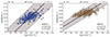 |
Fig. B.1. STFR and BTFR computed using the total masses instead of the stellar and baryonic masses contained within Rout. The color codes are given in the legend of the plot. |
The results of BTFR are rather surprising as they suggest that low-mass galaxies at high redshifts are highly gas-dominated systems. The later is previously suggested in Tacconi et al. (2020). However, given the shallowness of the relation, we underscore the need for accurate estimates of gas mass at high redshift. Most likely, the limitations lie in the HI scaling relations, which appear insufficient to constrain the total HI mass at high redshift. For these reasons, we do not report STFR and BTFR from the total mass in the main text. However, it could also be attributed to the lack of deep observations, potentially resulting in incomplete mapping of the circular velocity in low-mass galaxies, as reported in the latest study of Sharma et al. (2023). Most likely, high-resolution (deep integration time) observations are required to put tighter constrains on TFR at high redshift.
Appendix C: Tailored comparison of STFR and BTFR with high-z studies
As discussed in Sect. 2, the GS23 sample represents a rotation-supported system, lies on and around the main sequence of star-forming galaxies, and adheres to fundamental scaling relations (see Fig. 4). This suggests that the TFR of the full GS23 sample can be directly compared with local TFR studies as shown in Fig. 8. As well as to keep the consistency with respect to the sample selection between the local and the high-z Universe, we compare TFR of full GS23 sample with previous high-z studies as shown in Figs. 9 and 10.
However, it is evident from the works of previous high-z studies, namely Tiley et al. (2019) and Übler et al. (2017), that their sample selection, measurements of stellar and gas mass, and fitting techniques differ from those employed in local studies, as well as being discrepant from our approach. Therefore, in this section, we briefly discuss the physical properties of the aforementioned studies that are relevant to the TFR, emphasize their sample selection, and then compare their TFR fits with our datasets. In particular, Tiley et al. (2019) study is compared with KROSS sample and Übler et al. (2017) with KMOS3D sample.
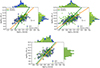 |
Fig. C.1. Comparison of the STFR, using only KROSS sample studied in GS23 datasets, with Tiley et al. (2019). The orange and green lines represent the best fit lines for our and Tiley et al. (2019)’s work, respectively. The blue and green data points represent- Upper Left Panel: Disk-like galaxies characterized by Vrot/σ > 3, Upper Right Panel: Rotation supported galaxies characterized by Vrot/σ > 1, and Lower Panel: KROSS and Tiley et al. (2019) matching sample for Vrot/σ > 1. We note that in this comparison, we used a rotation velocity with in Rout (i.e., Vrot), which is not corrected for pressure support; namely, Vrot is comparable to V2.2 of Tiley et al. (2019). |
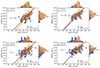 |
Fig. C.2. Comparison of the STFR and BTFR, using only KMOS3D sample studied in GS23 datasets, with Übler et al. (2017). In the top panel figures, we restrict the analysis for |

Comparison with Tiley+19: Following Harrison et al. (2017), Tiley et al. constructed line-of-sight velocity maps using Hα emission. To determine the rotation velocity of the system, a 0.7″ slit was placed along the major axis of the velocity map, enabling them to determine the rotation velocity using dynamical modeling based on the arctangent disk model (Courteau 1997). Subsequently, rotation curves were corrected for beam-smearing using the prescription outlined in Johnson et al. (2018). We note that their rotation curves are not corrected for pressure support; therefore, when comparing STFR, we use the rotation velocity of the GS23 sample instead of circular velocity (which incorporates pressure support corrections). The stellar masses of AT19 sample are derived using SED-fitting with the LEPHARE code (Arnouts et al. 1999; Ilbert et al. 2006) as discussed in Tiley et al. (2019). In this work, we utilize the same stellar masses received through private correspondence with Alfred Tiley. The study by Tiley et al. (2019) focuses only on STFR for two distinct cases: (1) a disky sample characterized by Vrot/σ > 3, and (2) a rotation-supported sample, i.e., Vrot/σ > 1. We compare our sample and its best fit to both cases, as illustrated in Fig. C.1, with the upper left and right panels representing the disky and rotation-supported samples, respectively.
In case of disky sample, upper left panel of Fig. C.1, we notice that AT19 sample is dominant toward massive systems (hence fast rotating). Conversely, the GS23 sample contains a larger dynamic range in velocities, i.e., also the lower velocities (low masses). This discrepancy is most-likely due to the capability of 3D forward modeling to account for low-mass systems, which are often overlooked in 2D kinematic modeling. Our analysis yields a slope of 3.20 ± 0.48, diverging by a factor of 2.0 from the slope observed in AT19. This difference is yet again attributed to variances in kinematic modeling and fitting methodologies, which likely contribute to the shallow slope and distinct offset in our work.
In the case of rotation-supported systems (upper right panel), the distributions of both samples match very closely in terms of velocity and stellar masses, as expected. However, there is a notable discrepancy in the best-fit relation. In particular, our slope of 2.29 ± 0.22 differs from Tiley et al. (2019) by a factor of 1.14 dex. To understand this discrepancy, we matched the AT19 and KROSS samples from Sharma et al. (2021), finding 96 matches, as shown in the bottom panel of Fig. C.1. We noticed that the discrepancy is only in terms of velocity estimates. When we fit this matched data of AT19 and GS23 using the orthogonal likelihood fitting technique, we obtained similar slopes that differ only in terms of offset due to differences in velocity estimates. This suggests that the discrepancy in the slope between AT19 and this work arises mainly from the fitting techniques. However, a minor difference could also stem from variations in beam-smearing corrections, which are implemented differently in both studies, or from the circular velocity measurements which are taken at different radii.
Comparison with Ubler+17.: In accordance with Wuyts et al. (2016), Übler et al. (2017) determined the radial velocity and velocity dispersion of the KMOS3D sample by placing a circular aperture with a diameter of 0.8″ along the kinematic major axis, utilizing the LINEFIT code (Davies et al. 2009), which considers spectral resolution. To obtain circular velocity profiles (rotation curves) for the system, they employed dynamic mass modeling of kinematic profiles using DYSMAL (Cresci et al. 2009; Davies et al. 2011), allowing for an exponential disk with a Sersic index of ns = 1. This modeling procedure encompasses the coupled treatment of radial velocity and velocity dispersion, incorporating beam-smearing (see, Davies et al. 2009, 2011) and pressure support correction assuming constant and isotropic velocity dispersion (Burkert et al. 2010).
It is crucial to note that Sharma et al. (2023) employs 3DBarolo to estimate circular velocity profiles, utilizing a non-parametric approach while simultaneously correcting for spectral and spatial resolution (i.e., beam-smearing) in 3D space. Subsequently, these rotation curves (rotation curves) underwent pressure support corrections, as detailed in Sharma et al. (2021), following the methodology of Weijmans et al. (2008). In the latter, pressure support corrections do not assume constant and isotropic velocity dispersion unlike Burkert et al. (2010); instead, they account for velocity anisotropies. For further details we refer to Sharma et al. (2021) and Sharma et al. (2023).
The star-formation rates and stellar masses in Übler et al. (2017) are estimated through proper SED fitting techniques discussed in Wuyts et al. (2011), Wisnioski et al. (2015), and Wisnioski et al. (2019). Molecular mass estimates are obtained using the scaling relation of Tacconi et al. (2018). The HI gas mass is considered negligible within 1 − 3Re, i.e., Mbar = M⋆ + MH2. However, following Burkert et al. (2016), the author applied larger uncertainties (0.2 dex) to total gas mass measurements to account for missing HI mass. In comparison, Sharma et al. (2023) consider Mbar = M⋆ + MH2 + MHI, where the estimates for stellar and molecular gas mass align with those of Übler et al. (2017). However, the HI mass is derived using a scaling relation. Further details on baryonic mass estimates are provided in Sect. 2.2.
In terms of sample selection, Übler et al. (2017) focuses on galaxies on-and-around the main-sequence of star-forming galaxies. However, to select the most disk-like systems, they apply a  cut and then study the STFR and BTFR. To facilitate one-to-one comparison of our fitting techniques, we select only KMOS3D sample from GS23 and apply a
  cut, resulting in 53 remaining galaxies. We show the results of this tailored comparison in Fig. C.2, with the STFR in the left panel and the BTFR in the right panel. Notably, the distribution of stellar/baryonic mass and circular velocities is skewed in our sub-sample. In contrast, the Übler et al. (2017) sample comprises 135 galaxies with a Gaussian distribution in both mass and velocities. In the GS23 sub-sample, the median circular velocity is approximately 150 km/s, with a stellar mass of ∼109.7 M⊙ and a baryonic mass of ∼1010.3 M⊙. Conversely, in the Übler et al. (2017) sample, the median circular velocities are around 250 km/s, with stellar and gas masses at ∼1010.5 M⊙. For this tailored comparison, our sample is biased toward intermediate-mass systems, while the Übler et al. (2017) sample consists mainly massive systems.
To fit the STFR and BTFR of the GS23 KMOS3D sub-sample, we employ the same techniques established in Appendix A and applied in Sect. 3. The results are presented in Fig. C.2. For the STFR, we report a slope of  , intercept
  , intrinsic scatter of 0.15 dex. For the BTFR, the reported values for the slope is
  , intercept corresponds to
  , and an intrinsic scatter of 0.14 dex.
It is evident that at fixed stellar or baryonic mass, the circular velocity in Übler et al. (2017) sample is higher by factors of 1.3-1.5. This is most-likely due to their pressure support correction method that assumes constant and isotropic velocity dispersion, which overestimates the circular velocity across the galactic scales. Additionally, we compare the STFR and BTFR of full KMOS3D sample of GS23 with Übler et al. (2017) in second row of Fig. C.2. Nevertheless, we encountered the similar evolution in TFR slopes. This suggests that differences are arising due to difference in kinematic modeling and fitting techniques employed in our work.
Appendix D: Fits with vertical scatter
In this section we briefly discuss the results obtained using vertical likelihood that minimizes the intrinsic scatter in the vertical direction as defined in Eq. (A.1). In Fig. D.1, we show the best-fit and corner plots for the STFR and BTFR on the full GS23 dataset in the left and right panels respectively. For STFR, we report α = 1.31 ± 0.10, β = 7.063 ± 0.21 and ζint = 0.097. Similarly for BTFR we find, α = 1.23 ± 0.1, β = 7.46 ± 0.22 and ζint = 0.15. It is interesting to note that the slopes for the STFR and BTFR differ from the orthogonal best fit slopes by 1.72 dex and 1.98 dex respectively.
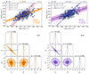 |
Fig. D.1. Stellar and baryonic Tully-Fisher relations (STFR and BTFR) obtained using a vertical likelihood method, presented in the left and right panels of the upper panel, respectively. The blue filled circles represent the data from Sharma et al. (2023), with gray error bars denoting uncertainties on each measurements. The solid orange and purple lines shows the best-fit curves obtained in this study, accompanied by the shaded regions representing the 3σ intrinsic scatter for the STFR and BTFR, respectively. The bottom right corner of each plot displays the best-fit parameters. Additionally, the blue lines correspond to comparisons with local studies, while red lines represent the high-redshift data, as indicated in the upper left legend of each plot. Lower Panel: Posterior distributions (corner plots) resulting from the MCMC fitting process for the STFR and BTFR are shown in the left and right plots, respectively. The contours within these corner plots illustrate the 68%, 90%, and 99% credible intervals. |
All Tables
The slopes of STFR and BTFR obtained in this work along with a comparison to previous studies.
All Figures
|
Fig. 1. Main sequence of local star-forming galaxies is shown by solid blue line and for redshifts of 1.0, 1.5, and 2.0, shown by blue, pink, and red shaded areas, respectively. The KMOS3D, KGES and KROSS data is shown by red, green, and blue filled circles. Hereafter, we refer this to full dataset as GS23 and depict in blue color throughout the work. |
| In the text | |
|
Fig. 2. Comparison of circular velocities, VcRout and Vmax. The black solid line shows the one-to-one relation followed by dashed lines showing the 1σ intrinsic scatter around this line. Since the measurements of VcRout and Vmax correlate within 1σ, it suggests that both velocity measurements are good proxies for circular velocity of galaxies. In the analysis, we refer to VcRout = Vc as the circular velocity of the object. |
| In the text | |
|
Fig. 3. Intrinsic and pressure-support-corrected rotation-to-dispersion ratio (V/σ), plotted on the y- and x-axes, respectively. The solid black line represents the one-to-one relation between the two quantities. The vertical and horizontal dashed lines indicate the V/σ > 1 limit for intrinsic and pressure-support-corrected rotation-to-dispersion ratios, respectively. This figure indicates that, after pressure support corrections, none of the GS23 galaxies exhibit dispersion-dominated characteristics. Therefore, we utilize the entire GS23 sample for the TFR study. |
| In the text | |
|
Fig. 4. Mass-size relation of late-type galaxies (left). The blue filled circles represents the data (of Sharma et al. 2023, employed in this work), and black dashed line shows the best-fit (slope and offset marked on plot). The blue and red shaded areas represent the mass-size relation of van der Wel et al. (2014) at z = 0.75 and z = 2.25, respectively. Ionized gas velocity dispersion as a function of redshift (right). The blue filled circles and brown hexagons represent the Sharma et al. (2023) and Übler et al. (2019) data, respectively. The brown dashed line represents the best fit of Übler et al. (2019) work. We notice that 73 out of the 263 (27.7%) galaxies from the Sharma et al. (2023) sample are common in the two datasets. |
| In the text | |
|
Fig. 5. Stellar and baryonic Tully-Fisher relations (STFR and BTFR), presented in the top-left and top-right panels, respectively. The blue-filled circles represent the data from Sharma et al. (2023), with gray error bars denoting uncertainties on each measurements. The solid orange and purple lines shows the best-fit curves obtained in this study using orthogonal likelihood, accompanied by the shaded regions representing the 3σ intrinsic scatter for the STFR and BTFR, respectively. The bottom-right corner of each plot displays the best-fit parameters. Additionally, the blue lines correspond to comparisons with local studies, while red lines represent the high-redshift data, as indicated in the upper left legend of each plot. The lower panel shows the posterior distributions (corner plots) resulting from the MCMC fitting process for the STFR and BTFR, shown in the left and right plots, respectively. The contours within these corner plots illustrate the 68%, 90%, and 99% credible intervals. For reference, we also show vertical likelihood fits of STFR and BTFR in Fig. D.1, which shows a huge difference in the slope and zero-point of the relation with respect to orthogonal likelihood. We report a difference of a factor of about 2. |
| In the text | |
|
Fig. 6. Comparison of slopes and intrinsic scatters: we take the best-fits of previous studies as a face-value (x-axis) and apply them on our dataset to compute the orthogonal intrinsic scatter (y-axis) around the adopted best-fit lines. STFR studies are represented by orange markers, BTFR studies by purple, with each marker corresponding to a distinct study listed in the legends. |
| In the text | |
|
Fig. 7. STFR and BTFR, respectively, separated into two redshift bins: 0.6 ≤ z ≤ 1.2 ( |
| In the text | |
|
Fig. 8. Comparison of STFR and BTFR with local studies. Left Panel: STFR comparison between the GS23 dataset (blue filled circles) and Lapi2018 (gray open circles). The best fit for Lapi2018 is represented by the black solid line, while the best-fit of this work (on GS23 data) is shown in orange. Right Panel: BTFR comparison between the GS23 dataset (blue filled circles) and Lelli2019 (brown open circles). The best fit for Lelli2019 is indicated by the brown solid line, while the best-fit of this work in purple. In both panels, the inset provides a zoomed-in view of the local and high-z fits within the range 9.0 ≤ log(Mstar/bar [M⊙]) ≤ 11.5 and 1.65 ≤ log(Vc [km/s]) ≤ 2.75. Additionally, for dataset comparison, histograms of the x and y axes are included: Lapi2018 in gray, Lelli2019 in brown and GS23 in blue. In both the STFR and BTFR cases, we observe a divergent evolution in the slope, while the zero-point remains uncertain due to the absence of low-mass galaxies at high redshifts. |
| In the text | |
|
Fig. 9. Comparison of STFR data of this work with datasets of other high-redshift studies: Tiley et al. (2019, green squares) and Übler et al. (2017, brown hexagons). The orange, green, and brown lines represent the best-fit results for our study, Tiley et al. (2019), and Übler et al. (2017), respectively. To facilitate a comprehensive comparison of the datasets, we provide histograms showing the distributions of stellar mass and circular velocities, both horizontally and vertically, color-coded same as their respective datasets. We note that the velocities for Tiley et al. (2019) are rotational velocities and not circular velocities. |
| In the text | |
|
Fig. 10. Comparison of BTFR dataset of this study with Übler et al. (2017, brown hexagons). The purple and brown lines represent the best-fit results for our study and Übler et al. (2017), respectively. For a comprehensive comparison of the datasets, we provide histograms showing the distributions of stellar mass and circular velocities, both horizontally and vertically, color-coded according to their respective datasets. |
| In the text | |
|
Fig. A.1. Vertical and orthogonal likelihood fitting on mock data resembling the local stellar and baryonic Tully-Fisher datasets. Upper Panel: Mock dataset depicted as open black circles with errors, accompanied by the best-fit lines. The solid black line represents the true slope of 3.5 used for generating the mock data. The blue and red solid lines correspond to the best fits obtained using the vertical and orthogonal likelihood methods, respectively. Both best-fit lines are followed by 3σ intrinsic scatter regions, indicated with the same color code as the best fits. Lower Panel: Posterior distributions resulting from MCMC-fitting for the vertical and orthogonal likelihoods are shown in blue and red, respectively. The contours within these corner plots illustrates the 68%, 90%, and 99% credible intervals. |
| In the text | |
|
Fig. A.2. Vertical and orthogonal likelihood fitting on mock data resembling the high-redshift stellar and baryonic Tully-Fisher relations. Left Panel: Mock dataset depicted as open black circles with associated errors, accompanied by the best-fit lines. The solid black line represents the true slope of 3.5 used for generating the mock data. The blue and red solid lines correspond to the best fits obtained using the vertical and orthogonal likelihood methods, respectively. Both best-fit lines are followed by 3σ intrinsic scatter regions, indicated with the same color code as the best fits. Right Panel: Posterior distributions resulting from the MCMC fitting process for the vertical and orthogonal likelihoods are shown in blue and red, respectively. The contours within these corner plots illustrates the 68%, 90%, and 99% credible intervals. |
| In the text | |
|
Fig. B.1. STFR and BTFR computed using the total masses instead of the stellar and baryonic masses contained within Rout. The color codes are given in the legend of the plot. |
| In the text | |
|
Fig. C.1. Comparison of the STFR, using only KROSS sample studied in GS23 datasets, with Tiley et al. (2019). The orange and green lines represent the best fit lines for our and Tiley et al. (2019)’s work, respectively. The blue and green data points represent- Upper Left Panel: Disk-like galaxies characterized by Vrot/σ > 3, Upper Right Panel: Rotation supported galaxies characterized by Vrot/σ > 1, and Lower Panel: KROSS and Tiley et al. (2019) matching sample for Vrot/σ > 1. We note that in this comparison, we used a rotation velocity with in Rout (i.e., Vrot), which is not corrected for pressure support; namely, Vrot is comparable to V2.2 of Tiley et al. (2019). |
| In the text | |
|
Fig. C.2. Comparison of the STFR and BTFR, using only KMOS3D sample studied in GS23 datasets, with Übler et al. (2017). In the top panel figures, we restrict the analysis for |
| In the text | |
|
Fig. D.1. Stellar and baryonic Tully-Fisher relations (STFR and BTFR) obtained using a vertical likelihood method, presented in the left and right panels of the upper panel, respectively. The blue filled circles represent the data from Sharma et al. (2023), with gray error bars denoting uncertainties on each measurements. The solid orange and purple lines shows the best-fit curves obtained in this study, accompanied by the shaded regions representing the 3σ intrinsic scatter for the STFR and BTFR, respectively. The bottom right corner of each plot displays the best-fit parameters. Additionally, the blue lines correspond to comparisons with local studies, while red lines represent the high-redshift data, as indicated in the upper left legend of each plot. Lower Panel: Posterior distributions (corner plots) resulting from the MCMC fitting process for the STFR and BTFR are shown in the left and right plots, respectively. The contours within these corner plots illustrate the 68%, 90%, and 99% credible intervals. |
| In the text | |
Current usage metrics show cumulative count of Article Views (full-text article views including HTML views, PDF and ePub downloads, according to the available data) and Abstracts Views on Vision4Press platform.
Data correspond to usage on the plateform after 2015. The current usage metrics is available 48-96 hours after online publication and is updated daily on week days.
Initial download of the metrics may take a while.