| Issue |
A&A
Volume 652, August 2021
|
|
|---|---|---|
| Article Number | A95 | |
| Number of page(s) | 47 | |
| Section | Stellar structure and evolution | |
| DOI | https://doi.org/10.1051/0004-6361/202040272 | |
| Published online | 17 August 2021 | |
Revisiting the archetypical wind accretor Vela X-1 in depth
Case study of a well-known X-ray binary and the limits of our knowledge
1
European Space Agency (ESA), European Space Astronomy Centre (ESAC), Camino Bajo del Castillo s/n, 28692 Villanueva de la Cañada, Madrid, Spain
e-mail: Peter.Kretschmar@esa.int
2
Institut de Planétologie et d’Astrophysique de Grenoble, 414 Rue de la Piscine, 38400 Saint-Martin-d’Hères, France
e-mail: ileyk.elmellah@univ-grenoble-alpes.fr
3
Centre for Mathematical Plasma Astrophysics, KU Leuven, Celestijnenlaan 200B, 3001 Leuven, Belgium
4
Institute of Astronomy, KU Leuven, 3001 Leuven, Belgium
5
Instituto de Física de Cantabria (CSIC-Universidad de Cantabria), 39005 Santander, Spain
6
Quasar Science Resources S.L for European Space Agency (ESA), European Space Astronomy Centre (ESAC), Camino Bajo del Castillo s/n, 28692 Villanueva de la Cañada, Madrid, Spain
7
Institut für Astronomie und Astrophysik (IAAT), Universität Tübingen, Sand 1, 72076 Tübingen, Germany
8
Armagh Observatory and Planetarium, College Hill, Armagh, BT61 9DG Northern Ireland, UK
9
Anton Pannekoek Institute for Astronomy, University of Amsterdam, Science Park 904, 1098 XH, Amsterdam, The Netherlands
10
Department of Physics, Astrophysics, University of Oxford, Oxford, UK
11
Centro de Astrobiología, CSIC-INTA, Campus ESAC, Camino bajo del castillo s/n, 28692 Villanueva de la Cañada, Spain
12
Vitrociset Belgium for European Space Agency (ESA), European Space Astronomy Centre (ESAC), Camino Bajo del Castillo s/n, 28692 Villanueva de la Cañada, Madrid, Spain
13
Aurora Technology BV for European Space Agency (ESA), European Space Astronomy Centre (ESAC), Camino Bajo del Castillo s/n, 28692 Villanueva de la Cañada, Madrid, Spain
Received:
31
December
2020
Accepted:
21
April
2021
Context. The Vela X-1 system is one of the best-studied X-ray binaries because it was detected early, has persistent X-ray emission, and a rich phenomenology at many wavelengths. The system is frequently quoted as the archetype of wind-accreting high-mass X-ray binaries, and its parameters are referred to as typical examples. Specific values for these parameters have frequently been used in subsequent studies, however, without full consideration of alternatives in the literature, even more so when results from one field of astronomy (e.g., stellar wind parameters) are used in another (e.g., X-ray astronomy). The issues and considerations discussed here for this specific, very well-known example will apply to various other X-ray binaries and to the study of their physics.
Aims. We provide a robust compilation and synthesis of the accumulated knowledge about Vela X-1 as a solid baseline for future studies, adding new information where available. Because this overview is targeted at a broader readership, we include more background information on the physics of the system and on methods than is usually done. We also attempt to identify specific avenues of future research that could help to clarify open questions or determine certain parameters better than is currently possible.
Methods. We explore the vast literature for Vela X-1 and on modeling efforts based on this system or close analogs. We describe the evolution of our knowledge of the system over the decades and provide overview information on the essential parameters. We also add information derived from public data or catalogs to the data taken from the literature, especially data from the Gaia EDR3 release.
Results. We derive an updated distance to Vela X-1 and update the spectral classification for HD 77518. At least around periastron, the supergiant star may be very close to filling its Roche lobe. Constraints on the clumpiness of the stellar wind from the supergiant star have improved, but discrepancies persist. The orbit is in general very well determined, but a slight difference exists between the latest ephemerides. The orbital inclination remains the least certain factor and contributes significantly to the uncertainty in the neutron star mass. Estimates for the stellar wind terminal velocity and acceleration law have evolved strongly toward lower velocities over the years. Recent results with wind velocities at the orbital distance in the range of or lower than the orbital velocity of the neutron star support the idea of transient wind-captured disks around the neutron star magnetosphere, for which observational and theoretical indications have emerged. Hydrodynamic models and observations are consistent with an accretion wake trailing the neutron star.
Conclusions. With its extremely rich multiwavelength observational data and wealth of related theoretical studies, Vela X-1 is an excellent laboratory for exploring the physics of accreting X-ray binaries, especially in high-mass systems. Nevertheless, much room remains to improve the accumulated knowledge. On the observational side, well-coordinated multiwavelength observations and observing campaigns addressing the intrinsic variability are required. New opportunities will arise through new instrumentation, from optical and near-infrared interferometry to the upcoming X-ray calorimeters and X-ray polarimeters. Improved models of the stellar wind and flow of matter should account for the non-negligible effect of the orbital eccentricity and the nonspherical shape of HD 77581. There is a need for realistic multidimensional models of radiative transfer in the UV and X-rays in order to better understand the wind acceleration and effect of ionization, but these models remain very challenging. Improved magnetohydrodynamic models covering a wide range of scales are required to improve our understanding of the plasma-magnetosphere coupling, and they are thus a key factor for understanding the variability of the X-ray flux and the torques applied to the neutron star. A full characterization of the X-ray emission from the accretion column remains another so far unsolved challenge.
Key words: X-rays: individuals: Vela X-1 / X-rays: binaries / stars: winds, outflows / accretion, accretion disks
© P. Kretschmar et al. 2021
 Open Access article, published by EDP Sciences, under the terms of the Creative Commons Attribution License (https://creativecommons.org/licenses/by/4.0), which permits unrestricted use, distribution, and reproduction in any medium, provided the original work is properly cited.
1. Introduction
Vela X-1 (4U 0900−40) is an eclipsing high-mass X-ray binary (HMXB) at a distance of about 2 kpc (Sect. 5.1). The binary system consists of an accreting neutron star that emits X-ray pulses with a period of ∼283 s (Sect. 3.1.6) in a close, mildly eccentric orbit with a period of ∼8.964 days (Sect. 5.2, Table 3) around the supergiant HD 77581, also known as GP Vel, which is most frequently described as B0.5 Ia supergiant. Because the orbital separation of ∼1.7R⋆ (Sect. 5.2) is small, the accreting neutron star is deeply embedded in the dense stellar wind of the supergiant star, with a mass loss of about 10−6 M⊙ yr−1 (Sect. 5.6). Figure 1 illustrates the system geometry. In this figure and in the remainder of this paper, the orbital phases quoted are expressed with respect to the mid-eclipse time Tecl defined in Kreykenbohm et al. (2008) as zero-point; the different ephemerides used in the literature are discussed in Sect. 5.2. The orbital eccentricity is high enough for the orbital phase 0.5 to be reached significantly after inferior conjunction of the neutron star. This detail is sometimes ignored when the system with its “almost circular” orbit is discussed.
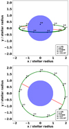 |
Fig. 1. Top panel: sketch of the Vela X-1 system as seen from Earth based on the ephemeris of Kreykenbohm et al. (2008), using an intermediate assumed inclination within the known constraints (see Sect. 5.3 and Table 4). Points mark the position of the neutron star at given orbital phases. Bottom panel: top view of the system. |
The intrinsic X-ray luminosity of Vela X-1 is only moderate (∼4 × 1036 erg s−1Nagase et al. 1986), but because of its proximity, it is still one of the brightest persistent point sources in the X-ray sky. Together with a wide variety of interesting phenomenology, this has made Vela X-1 a well-studied target ever since its detection. It has frequently been called an “archetype” of wind-accreting HMXB.
Because of its eclipsing nature, the extent of the donor star with respect to the orbital separation is well constrained, and so is the mass transfer mechanism. Because the orbit of the slowly spinning neutron star around its blue supergiant companion is almost circular (e ∼ 0.0898), the stellar line-driven wind provides a continuous source of material to the compact object. The sources of stochastic variability of the intrinsic X-ray emission induced by, for instance, overdense small-scale regions in the wind (hereafter called clumps), can be isolated from the orbital modulation. The cooperative behavior of Vela X-1 from an observational and theoretical point of view has made it a privileged target of study for modelers, as further detailed in Sect. 4.
As an example of a high-mass neutron star, with a mass that has been determined to be clearly higher than the Chandrasekar limit (Sect. 5.3), Vela X-1 is also frequently used as an example for models of compact stars and equation-of-state calculations or studies of neutron star mass distributions (e.g., Gangopadhyay et al. 2013; Özel & Freire 2016; Mafa Takisa et al. 2017; Gedela et al. 2019). Over the years, however, the knowledge about many system parameters has evolved, and different authors have used different conventions to report their results. Even more importantly, quite different assumptions about essential parameters of the system have been used by different authors in the interpretation of their observations or in their modeling, for instance, the velocity profile of the stellar wind, the nature and shape of larger structures, clumps and their parameters, or the role of ionization.
In this article we revisit a large sample of observational findings. We treat the information in a consistent manner as far as possible, and we compare the observations with information obtained from recent detailed modeling, especially of the wind structure (Sander et al. 2018) and of the flow of matter around the neutron star (El Mellah et al. 2018). The remainder of this paper is structured as follows: Sect. 2 summarizes the different elements of the Vela X-1 system in order to describe the framework in which observational diagnostics and modeling studies take place. Section 3 gives an overview of the observational diagnostics at different wavelengths and describes which parts of the system they explore. Section 4 describes semianalytical and numerical models of Vela X-1 or close analogs, and each time we pay particular attention to how different physical ingredients are handled. Section 5 summarizes the knowledge about basic system properties, as found in the literature, with an emphasis on clearly describing the differences between the results obtained in different studies. In Sect. 6 we give our view on how further observations and modeling efforts may help us to answer the open questions and add to our knowledge of this prototype system. Finally, Sect. 7 summarizes the essential points we raised throughout this overview.
2. Elements of the Vela X-1 system
The rich observational phenomenology of an HMXB system such as Vela X-1 is the result of a complex interplay of its various elements, where the relevant physics cover more than six orders of magnitude in size, as indicated in Fig. 2. In the following we describe these elements from larger to smaller size scales. For the sake of clarity, we introduce the main physical concepts relevant to this and similar systems when we discuss observations and modeling efforts in later sections. For a more complete discussion of stellar wind and HMXB physics see, for example, Martínez-Núñez et al. (2017).
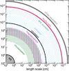 |
Fig. 2. Overview of characteristic length scales in the Vela X-1 system. Some of them are relatively well determined, on the order of 10%, and can be considered effectively fixed over the timescale of known observations. Other scales, shown with different types of hatching or shading, strongly depend on different parameters, as explained in the text. They may vary on short timescales of sometimes over an order of a magnitude or more, and a variation in one may drive changes in another. The ranges shown in this figure for these parameters are only to be taken as indicative. For comparison, the orbital separation corresponds to approximately 1/4 AU. |
2.1. Supergiant and its stellar wind
HD 77581 looses significant mass through a line-driven wind whose launching mechanism, first identified by Lucy & Solomon (1970) and Castor et al. (1975), relies on the resonant line-absorption of UV photons by partly ionized metal ions. The amount of mass lost and the intrinsic acceleration by the radiative field of the supergiant evidently strongly depend on parameters such as temperature, luminosity, radius, mass, and effective surface gravity, which are in themselves not perfectly well known; see Sects. 5.3 and 5.6. One major factor of uncertainty is that the effective temperature of the supergiant star (about 25 000 K, as found in most studies; see Table 5), lies in a sharp transition called the bistability jump between slow winds on the cool side and fast winds on the hot side (Vink et al. 1999).
In a spherically symmetric configuration, theoretical arguments and observational insights support a velocity profile for line-driven winds that follows a so-called β-law (Puls et al. 2008),
with R⋆ the stellar photosphere radius, v∞ the terminal wind speed, and β a positive exponent: its value determines how quickly the wind reaches v∞, with a more gradual acceleration for a higher value of β. In the case of Vela X-1, quite different values for v∞ (< 400 to ∼1700 km s−1) and β (0.8 to ∼2.2) have been reported by different authors, and the usefulness of a β-law as a description has been questioned (Sect. 5.6).
In line-driven winds, internal shocks are prone to develop because of the line-deshadowing instability (Lucy & White 1980; Owocki & Rybicki 1984). The local density departs from the smooth wind value, with an overall density ratio of ∼100 between the most and least dense regions at a given distance from the donor star. In the case of Vela X-1, current work (see Sect. 4.1 for details and references) suggests that at one stellar radius above the photosphere, most of the wind mass is contained in clumps. This wind clumping has often not been taken into account for discussions of the overall wind structure in the system. The internal shocks in line-driven winds that are responsible for the clump formation also produce X-rays, although the X-ray luminosity due to this process is low (∼1033 erg s−1). The sizes of clumps in stellar winds and in HMXBs have been estimated with widely varying ranges in the past (see the corresponding discussion in Martínez-Núñez et al. 2017). Recent simulations for hot and massive stars (Driessen et al. 2019) suggest that most of the wind mass is contained in clumps that are expected to appear as coherent structures of mass 1017−18 g and of a size of about 1% of the stellar radius. This is about 1010 cm for HD 77581.
The presence of the orbiting neutron star strongly affects the outflowing stellar wind through its gravity, the X-ray emission, and the orbital movement. Bessell et al. (1975) first highlighted the anisotropic distribution of material in the orbital plane induced by tidal forces, in agreement with the observational indications for a trailing wake that was reported in the early papers on Vela X-1 (see references in Conti 1978). As further described in Sect. 4.1, simulations of the Vela X-1 system (or close proxies) find a wind focused toward the neutron star, forming an unsteady bow shock that leads to an accretion wake. This wake trails the neutron star throughout its orbit (e.g, Blondin et al. 1991; Manousakis et al. 2012).
The line-driven acceleration of the stellar wind is affected by the intense X-ray emissions that are emitted from the immediate vicinity of the neutron star. This modifies the ionization structure of the wind in which it is embedded and thus the ability of the stellar radiative field to accelerate the wind through resonant line-absorption (Hatchett & McCray 1977). An additional ionizing contribution, which is expected to be very low for Vela X-1, however, may come from the X-rays that are produced in shocks in the wind. The local degree of ionization in an optically thin wind in thermal balance can be evaluated using the ionization parameter (Tarter et al. 1969),

where LX is the X-ray luminosity, n the local atomic number density of the gas, and rX the distance to the X-ray point source. Above a certain critical ionization parameter ξcrit, most of the elements responsible for the wind acceleration (e.g., C, N, O, and Fe) are expected to be fully ionized and the wind acceleration is essentially quenched. Depending on the shape of the irradiating X-ray spectrum and on the details of the resonant line-absorption mechanism, the value of ξcrit is expected to range between 102 and 104 erg cm s−1. Shocks between the radiatively driven wind and stagnant gas around the compact object can in principle lead to a trailing accretion wake (Fransson & Fabian 1980), but for Vela X-1 and similar systems, this is expected to be a lesser contribution to the gas density (Blondin et al. 1990). It is important to note, however, that the “on/off switch” for wind acceleration set by the critical ionization parameter is a simplifying assumption, as is further explained in the models that we present in Sect. 4.1.2. Moreover, wind clumping weakens the effect of X-ray ionization from the accreting compact object through the increased recombination inside the clumps (Oskinova et al. 2012).
Another large-scale feature that is common around massive hot stars are corotating interaction regions (Mullan 1984). None has been reported in Vela X-1, however.
2.2. Mass transfer to the neutron star
A fraction of the mass lost by HD 77581 is captured and accreted by the neutron star and fuels the intense X-ray emission. While the system is generally labeled a “wind accretor”, the exact mechanisms of mass transfer in the Vela X-1 system are not fully determined and have again become a topic of more intense research; see Sect. 4.2.1. Uncertainties remain on the orbital inclination, and to a lesser extent, on the mass ratio (Sect. 5.3), therefore it can currently not be excluded in principle that HD 77581 would fill its Roche lobe and thus lose mass through Roche-Lobe overflow (RLOF). However, the moderate X-ray luminosity of Vela X-1, the long and erratically varying spin period (Sect. 3.1.6), the absence of signatures for a permanent accretion disk, and the stable orbital period (Falanga et al. 2015) make an RLOF scenario very unlikely (see Sect. 4.2.1).
It is therefore generally assumed that the main mass transfer in Vela X-1 occurs through gravitational capture from the stellar wind. The length scale at which the wind is beamed toward the accretor by its gravitational field (on the order of the Roche-lobe radius of the neutron star) is much larger than the extent of the neutron star itself or its magnetosphere (see Fig. 2). In the fast-wind limit, the so-called Bondi–Hoyle–Littleton (BHL) formalism (Hoyle & Lyttleton 1939; Bondi & Hoyle 1944; Edgar 2004) provides a robust framework. In this description, the fraction of the wind with an impact parameter lower than the accretion radius Racc will be captured,
where MNS is the mass of the neutron star and vrel is the relative speed of the wind with respect to the neutron star. In this case, the mass accretion rate is approximately given by
where ρ is the wind density at the orbital separation. Subsequently, empirical refinements were proposed to correct vrel for slower winds (Davidson & Ostriker 1973). Still, the mass accretion rate is very sensitive to vrel, and to a lesser extent, to ρ, and a wide range of X-ray luminosities can be derived from smaller changes in these parameters, which are only relatively loosely constrained from observations and modeling (Sects. 4.1 and 5.6). In addition, the geometry of the problem itself might differ from the planar picture of the BHL framework because orbital effects are strong enough in Vela X-1 to significantly bend the flow to a point that it could form a disk-like structure before it reaches the magnetosphere.
2.3. Accretion close to and within the magnetosphere
The mass transfer rate is an upper limit on the mass accretion rate at the neutron star surface that eventually produces the observed X-ray luminosity. A fraction of the captured material could either stall in intermediate regions or might in principle be ejected, although there are no reports on outflows from close to the X-ray source in Vela X-1 so far (but see Sect. 3.3). When the flow reaches the magnetosphere, it is highly ionized by the intense X-ray flux that is emitted from the immediate vicinity of the neutron star surface. It behaves as a plasma, and its dynamic is entirely determined by the neutron star magnetic field, which channels the material all the way down to the neutron star magnetic poles (Davidson & Ostriker 1973).
For a qualitative understanding of the different possible accretion regimes within the magnetosphere, the following length scales play a role. First, the corotation radius which is the distance at which the neutron star magnetosphere, which rotates with the neutron star spin period, has the same angular velocity as the local Keplerian velocity. The mass, size, and spin period of the neutron star are fairly constant over timescales shorter than years, therefore the corotation radius can be considered as fixed. Second, the magnetospheric radius1 which is the distance to the neutron star below which the magnetic field dominates the dynamics of the inflowing plasma. A rigorous evaluation of this radius depends on the geometry of the inflow, but it is typically estimated by comparing the magnetic pressure to the ram pressure such that it increases with decreasing mass accretion rates. Other factors such as mass, radius, and magnetic field strength are again taken to be essentially fixed. Third, the circularization radius which is the radius of the Keplerian orbit that has the same specific angular momentum as the orbit of the accreted flow. Semianalytic and numerical estimates exist to evaluate the upper limit of the specific angular momentum of the inflow, but they vary by more than an order of magnitude between each other (Illarionov & Sunyaev 1975; Shapiro & Lightman 1976; Wang 1981; Livio et al. 1986).
Different estimates exist for the angular momentum accretion rate, but the upper limit commonly reads

where Ω = 2π/P is the angular orbital speed and P is the orbital period. We can then deduce the circularization radius,
where q is the ratio of the mass of the donor star to the mass of the neutron star, and a is the orbital separation. With realistic values for the orbital separation, the mass ratio, and the accretion radius, we obtain circularization radii in Vela X-1 that range between ∼5 × 107 cm and ∼2 × 109 cm for wind speeds at the orbital separation that range between 600 and 300 km s−1.
In the case of pure wind mass transfer, the flow carries a negligible amount of angular momentum, and the circularization radius is much smaller than the other two length scales (fast-wind case). A bow shock forms ahead of the neutron star with an opening angle smaller for higher Mach numbers of the inflow (El Mellah & Casse 2015). The flow is deflected by the shock, and provided its impact parameter is smaller than the accretion radius, it returns to the neutron star, essentially from the back hemisphere (for simulations of BHL accretion onto a magnetic dipole, see Toropina et al. 2012; Lee et al. 2014). If the mass accretion rate is high enough, the flow efficiently cools down downstream of the shock through bremsstrahlung or Compton processes, and the material freefalls at supersonic speeds onto the neutron star magnetosphere (Burnard et al. 1983). This regime is highly unsteady and is referred to as the direct accretion regime. Otherwise, the shock is adiabatic and the flow forms a quasi-spherical shell of hot material that subsonically settles onto the neutron star magnetosphere (Davies & Pringle 1981; Shakura et al. 2012). This regime has ramifications for different models depending on the intensity of the plasma-magnetosphere coupling (referred to as strong, moderate, and weak coupling in Shakura et al. 2012, 2018). In general, the plasma penetrates the magnetosphere through the interchange instability, which is the magnetohydrodynamics counterpart of the Rayleigh–Taylor instability (Arons & Lea 1976). For a more comprehensive description of the different accretion regimes onto a neutron star magnetosphere in wind-fed HMXBs in general, see Bozzo et al. (2008) and Martínez-Núñez et al. (2017).
For slower winds, the wind-RLOF mass transfer mechanism becomes more realistic. The bow shock extends up to a significant fraction of the Roche lobe of the neutron star (∼10%). As detailed in Sect. 4.2.1, in this regime, the accreted flow acquires and retains enough angular momentum through the shock so that the circularization radius is larger than the magnetospheric radius and a centrifugally maintained structure, called a wind-captured disk, can form within the shocked region. A disk like this would still be truncated at its inner edge by the magnetosphere, which is a few hundreds times larger than the neutron star radius, and thus such a disk would not radiate sufficiently at higher energies to be detected. Indirect evidence has emerged in recent years, however, for the existence of transient disks in wind-fed HMXBs in general (Hu et al. 2017; Taam et al. 2018; Taani et al. 2019) and for in Vela X-1 in particular (Liao et al. 2020). In this configuration, the disk and the magnetosphere are coupled by magnetic reconnection, the Kelvin–Helmholtz instability, and Bohm diffusion (Ghosh & Lamb 1979a). The ratio of the corotation radius and the magnetospheric radius then controls accretion and the transfer of angular momentum between the neutron star and the accreted matter. In the most simple cases, plasma that rotates faster at the magnetosphere than at the magnetic field lines that are anchored in the neutron star can dissipate kinetic energy, accrete, and spin the neutron star up, while at the other extreme, in the propeller regime, plasma that rotates more slowly than the magnetic field lines at the magnetosphere is expected to be expelled by the centrifugal force at the magnetocentrifugal barrier. This reduces the angular momentum of the neutron star (Illarionov & Sunyaev 1975). Intermediate cases are discussed in Ghosh & Lamb (1979a) and many publications based on this work (see Bozzo et al. 2009, for an overview and application to different sources). Strong torques for spin-up and spin-down can also be transmitted in quasi-spherical accretion (Shakura et al. 2012). A comparison of disk and quasi-spherical model predictions for various accreting pulsars is presented in Malacaria et al. (2020). The two geometries are sketched in Fig. 3, and the implications for Vela X-1 are further discussed in Sect. 4.2.2.
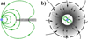 |
Fig. 3. Disk (a) and quasi-spherical (b) accretion geometries at the outer edge of the neutron star magnetosphere (represented in green as a dipole), adapted from Ghosh & Lamb (1978) and Shakura et al. (2012), respectively. In each of these ideal geometries, different accretion regimes are expected according to semianalytic derivations, depending on how the plasma couples to the magnetic field. |
2.4. Accretion column and X-ray emission
When the plasma has coupled to the magnetic field, it is funnelled to the magnetic poles of the neutron star where it forms a polar cap or accretion columns and emits most of the X-ray emission we observe (Davidson & Ostriker 1973; Lamb et al. 1973; Shapiro & Salpeter 1975; Arons et al. 1987). No hysteresis is expected in the sense that a given mass accretion rate will correspond to a specific X-ray luminosity (averaged over the spin period): The energy acquired by the flow in its journey from the stellar photosphere to the neutron star surface has to be released, except when there are significant outflows from the immediate vicinity of the neutron star. This has not been observed at this point. When the spin and magnetic axis of the neutron star are not aligned, which is frequently the case, regular pulses can be observed at the rotation frequency of the neutron star (see, e.g., the catalog of Liu et al. 2006, where 66 of 114 HMXBs in the Galaxy have an identified pulse period). The intensity and shape of the observable pulse profile, that is, the distinct pattern of the light curve folded with the pulse period, results from a complex interplay of multiple factors. The emission itself is expected to be nonuniform and is often highly beamed (Basko & Sunyaev 1975; Mushtukov et al. 2018). The emitted radiation is therefore strongly affected by relativistic light that in the curved space time bends close to the neutron star (e.g., Meszaros & Riffert 1988; Riffert & Meszaros 1988; Kraus et al. 1995; Odaka et al. 2014; Sotani & Miyamoto 2018; Falkner 2018, and references therein). Close to the neutron star surface, nondipolar components of the magnetic field might also have a significant effect on the dynamics of the plasma (Pétri 2015, 2017; de Lima et al. 2020). Even when the magnetic field is purely dipolar, there could be many regions on the neutron star surface to which the plasma is funnelled, and they do not necessarily correspond to the magnetic poles (Romanova et al. 2004).
The emitted X-ray spectrum of the column is dominated by Compton scattering of thermal seed photons. Cyclotron emission and scattering processes play an important role as well (Schwarm et al. 2017a,b, and references therein). A substantial fraction of accreting X-ray pulsars show relatively broad absorption line features in their X-ray spectra (see Staubert et al. 2019, for a recent review). These features result from resonant scattering of X-ray photons on electrons, whose energies perpendicular to the magnetic field are quantized into so-called Landau levels. This causes the plasma to become optically thick for X-ray photons at these energies and triggers the formation of cyclotron resonant scattering features (CRSFs) or often simply cyclotron lines. The spacing of these lines is determined by the energy difference between adjacent Landau levels, leading to centroid line energies of
where n is number of Landau levels involved in the scattering, z is the gravitational redshift due to the neutron star mass, e and me are the electron charge and mass, B is the magnetic field in the scattering region, c is the speed of light, and B12 is the magnetic field strength in units of 1012 Gauss. Determining cyclotron line energies thus gives a relatively direct measure of the magnetic field strength of the neutron star. CRSF studies for Vela X-1 are discussed in Sect. 3.1.5, and the implications for the neutron star magnetic field are summarized in Sect. 5.8.
Despite significant efforts and some progress, as further detailed in Sects. 4.3 and 4.4, there is currently no self-consistent, physics-based description that can correctly describe the spectra of accreting X-ray pulsars under all circumstances.
3. Observational diagnostics
In this section, we review the different methods which were used to constrain the parameters in Vela X-1. We treat the different wavelength domains separately.
3.1. X-ray diagnostics
3.1.1. Continuum spectrum
The X-ray luminosity of Vela X-1 is dominated by the X-ray continuum produced in the accretion column. For a distance of 2 kpc, the median luminosity is between 4 and 5 × 1036 erg s−1 in the 20–60 keV energy band (Nagase et al. 1986; Fürst et al. 2010). This approximately translates into a bolometric luminosity of about 1 × 1037 erg s−1. However, the Vela X-1 luminosity varies strongly (e.g., Kreykenbohm et al. 2008) and follows a log-normal distribution (Fürst et al. 2010). Figure 4 (top) shows the distribution of the observed hard flux, which is a good tracer of the intrinsic luminosity. Even on the day-long timescales sampled by Swift/BAT, large flares of 5–11 times the average luminosity are regularly observed.
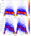 |
Fig. 4. Brightness distribution of Vela X-1 throughout its orbit as measured with Swift/BAT (15–50 keV, top panel) and MAXI (2–20 keV, bottom panel). In comparison, 1 Crab corresponds to values ∼0.22 for Swift/BAT and ∼4 for MAXI. We used the full history for each instrument, binned to a resolution of 1 d. The mean orbital flux profile is superimposed in black. The probability for a measurement to fall into the respective histogram bin is color-coded according to the color scales on the right. The profile is repeated once for clarity. For details, see text. |
The X-ray emission of Vela X-1 outside the eclipse can be phenomenologically described, as in many other accreting X-ray pulsars, by a power-law shape with a rollover at higher energies, beyond 15–30 keV (e.g., Nagase et al. 1986; Kreykenbohm et al. 1999; Orlandini et al. 1998; Odaka et al. 2013). However, the exact shape of this rollover is unknown. In the simplest approach, it can be modeled with an exponential cutoff alone, but observations with a high signal-to-noise ratio at energies beyond 30 keV often require a more complex shape of the rollover, and different phenomenological models have been used in the literature (e.g., Orlandini et al. 1998; Odaka et al. 2013). The continuum is modified at lower energies by variable amounts of absorption (see Sect. 7.2), a significant iron fluorescence line with an occasional iron edge (Nagase et al. 1986) and a frequent thermal soft excess below ∼3 keV (Sato et al. 1986; Pan et al. 1994; Haberl 1994), as well as further fluorescence lines from elements such as silicon, magnesium, and neon (e.g., Sako et al. 1999; Goldstein et al. 2004). At higher energies, the continuum is modified by CRSFs between 25 keV and 30 keV and at ∼55 keV, as further detailed in Sect. 3.1.5.
The overall continuum slope and the CRSFs vary strongly with the phase of the X-ray pulse (e.g., Kreykenbohm et al. 2002; La Barbera et al. 2003), but within the scope of this paper, we do not discuss this further.
During the eclipse, the residual X-ray emission shows no pulsations and is dominated by line emission in addition to a flat continuum Nagase et al. (1994), Schulz et al. (2002).
In general, the X-ray flux observed from Vela X-1 varies significantly in a largely random pattern around the mean value when the clearly visible X-ray eclipse is excluded. These variations are driven by variations in the intrinsic X-ray emission and by strong variations in the absorbing material between observers and the neutron star, especially for instruments in the soft X-ray band.
3.1.2. Eclipse timing
Despite the sparse observations of the time, it was soon realized in the early years after the detection that Vela X-1 was a variable source (Giacconi et al. 1972, and references therein). Based on long observations with the OSO-7 UCSD X-ray telescope, Ulmer et al. (1972) found evidence for periodic flux variations with phases of zero flux at a period of 8.7 ± 0.2 d and proposed that the X-ray source might be a member of an eclipsing binary system. This result was confirmed, and the periodicity was refined to 8.95 ± 0.02 d by Forman et al. (1973), based on Uhuru data. In subsequent years, the eclipse timing and derived orbital parameters were refined by various authors, for example, by Ögelman et al. (1977), using 20 days of COS-B data, or by Watson & Griffiths (1977), using Ariel V data covering 17 binary cycles, see Table 3. Most recently, Falanga et al. (2015) combined eclipse times derived from INTEGRAL observations with the earliest data to investigate a possible evolution of the orbital parameters (Sect. 5.2).
3.1.3. Variations in the X-ray absorption
Early observations of Vela X-1 (Eadie et al. 1975; Watson & Griffiths 1977; Becker et al. 1978) already found indications for significant and variable absorption in the system, together with brightness variations. Because of instrumental limitations, the brightness variations could not always be clearly ascribed to variations in absorbing material or in the intrinsic X-ray flux. Later observations with improved X-ray continuum spectra allowed better measurements of the actual absorption and found strong variability on many timescales. In Tenma data, Ohashi et al. (1984) found large variations of the absorbing column density NH that ranged from 2 to 50 × 1022 cm−2 on a timescale of about an hour.
Over the years, very many observations have among other properties followed the temporal evolution of the absorbing column density in the Vela X-1 system; see Fig. 5 and Table A.1. When they are presented in the same figure as a function of the orbital phase, different sets of NH measures can be misleading because they often do not belong to the same orbit and because the column density at a given orbital phase is not stable from one orbit to the next. The overall behavior can be summarized by the following statements. First, from orbital phase ϕorb ∼ 0.1 (eclipse egress) to ∼0.25, NH generally decreases strongly, often by more than one order of magnitude. This is usually explained by suggesting that the X-ray source shines through the extended atmosphere of its companion. Occasionally, shorter deviations from this trend have been found (Nagase et al. 1986; Martínez-Núñez et al. 2014). These are most probably caused by absorbing material closer to the X-ray source. Second, between ϕorb ∼ 0.25 and ∼0.6, strong variations of NH on timescales of hours to days are observed. At any given phase, high and low absorbing column densities have been found in different binary orbits, sometimes using the same instrument and analysis method (e.g., Nagase et al. 1986). This also applies to ϕorb ∼ 0.5, where Haberl & White (1990) and Watanabe et al. (2006) found high NH values, which the latter modeled as broad cold cloud, but where Nagase et al. (1986) found an intermediate minimum, as shown in Fig. 5. In a systematic study of MAXI data, Malacaria et al. (2016) found that ∼15% of all orbital light curves showed a dip around ϕorb ∼ 0.5, which was best explained by Thomson scattering in an extended and ionized accretion wake. Third, for late orbital phases (ϕorb > 0.6) up to the eclipse ingress, the observed absorbing column densities always remain high, but are still significantly variable by a factor of a few.
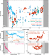 |
Fig. 5. Variations in derived absorbing column density (NH/cm2) throughout the binary orbit of Vela X-1 as determined by various observations and different satellites. See the text for caveats when absolute values in NH are compared. The shaded gray areas mark the eclipse (dark gray) and the ingress and egress (light gray) as determined by Sato et al. (1986). Binary phase values have been corrected for the differences in phase-zero definition (using Tecl) and orbital period relative to Kreykenbohm et al. (2008). The uncertainty in this conversion is 1–4 × 10⁻³ in phase, i.e., usually within the symbol size. Care has been taken to separate measurements taken during different binary orbits by the same instrument and team. Where possible, this is marked by different symbols. The data have been taken from Sato et al. (1986, Fig. 5 (Tenma)), Haberl & White (1990, Fig. 2 (EXOSAT)), Lewis et al. (1992, Fig. 2 (Ginga)), Pan et al. (1994, Fig. 3 (TTM/HEXE)), Watanabe et al. (2006, Table 2 (Chandra 2001)), Martínez-Núñez et al. (2014, Fig. 7 (XMM-Newton)) and Liao et al. (2020, Table 1 (Chandra 2017)). Panel a: an overview of the overall distribution, demonstrating the large scatter of results at intermediate orbital phases and that the larger structures driving NH are not stable from one orbit to the next (see also Malacaria et al. 2016). Panels b–e: subsets of the data in more detail to better visualize short-term variations. In all these panels, the X-axis covers the same range, and the Y-axis covers the same factor between minimum and maximum. |
The following caveats apply when results from different publications on the absolute values of NH are applied. First, spectral modeling results are usually somewhat degenerate for the parameters defining the spectral slope (e.g., a power-law index) versus the amount of absorbing material. The impact of this depends on the energy range that is covered, on the spectral response of each detector, and on the assumptions about permitted models in the fit procedure. For historical missions, it is frequently impossible to repeat the data reduction and analysis, even if time and knowledge were available for lack of suitable data in archives. Second and similarly, the inclusion or exclusion of an assumed soft excess can have a strong effect on the derived NH. Third, while many publications have used a single, unique absorbing column to obtain their results, in some particularly detailed studies, multiple absorption components were required to fit all of the available spectra (Haberl & White 1990; Martínez-Núñez et al. 2014). In this case, one absorbing component may have significantly higher NH values, but this only affects a fraction of the total observed radiation. Fourth, as detailed in Martínez-Núñez et al. (2017, Sect. 4.4.1) various different absorption models have been published in the literature and used over the years by different authors. These models rely on different assumptions for the interstellar medium cross-sections and abundances of the different elements, which can lead to differences of more than 20% in the obtained NH.
We show the effect of variable absorption on the spectrum of Vela X-1 in Fig. 6. In particular, we demonstrate that even a combination of relatively simple continuum models can lead to complex variability in spectral shape. To do so, we used the model that was introduced to describe the 0.5–10 keV spectrum of Vela X-1 by Martínez-Núñez et al. (2014), namely a sum of three power-law components that have different normalizations, but the same spectral index. Each of the power laws is absorbed by a distinct absorption component. A possible physical interpretation of this model is a complex partial coverer, possibly with an additional soft excess contribution (e.g., Grinberg et al. 2020). Martínez-Núñez et al. (2014) found that the main driver for the variable absorbed spectral shape of Vela X-1 during a flaring episode was the absorption of the second, most prominent power-law component. Figure 6 is calculated for typical values of the power-law index and relative power-law component contributions. It clearly shows how changes in absorption in this component can lead to strong nonlinear variability in the overall spectral shape.
 |
Fig. 6. Effect of variable absorption on the overall shape of the spectrum of Vela X-1 in the 0.5–10 keV range. Following Martínez-Núñez et al. (2014), we assume a spectral model consisting of three power-law components with the same slope, but different normalizations, each absorbed by a different absorption component. In accordance with trends seen by Martínez-Núñez et al. (2014), we then vary the total amount of absorption that the second of these power-law components experiences. The dot-dashed gray line shows the first power-law component. The dashed lines show the second power-law component, and different colors represent different absorption strengths, as indicated in the plot. The dot-dot-dashed line shows the third power-law component. The sum of the three components, i.e., the total spectrum, is shown as solid lines, and colors again represent different absorption levels for the second component. |
Grinberg et al. (2017) have explored a different temporal and spatial scale. In order to test the effect of clumps in the wind on short-term variations in the absorbing column density, they compared data from a Chandra observation of Vela X-1 at orbital phases ∼0.21 to ∼0.25 with a toy model that consisted of a constant X-ray source and a clumpy wind, based on the simulations by Sundqvist et al. (2018). They found that undisturbed inhomogeneities in the model wind could not account for the observed enhanced absorption (see also El Mellah et al. 2020b, for an extended model), indicating that more complex factors such as shock-clump interaction, the possibility of transient disk structures, or the effect of the compact object and its X-ray emission on the wind itself must be included.
3.1.4. X-ray polarization
For lack of sensitive X-ray polarimeters in space, no observations of X-ray polarization parameters in Vela X-1 or similar systems from X-ray satellites have so far been made. A notable recent exception was the balloon-borne hard X-ray calorimeter, X-Calibur, which observed Vela X-1. Because the flight duration was much shorter than anticipated, however, no constraining data could be obtained (Abarr et al. 2020).
Clear polarization signatures are expected from the physics of the radiation transfer in the emission region as well as in the system as a whole, however. Photon-scattering opacities within the accretion column will depend strongly on energy, on the direction of propagation, and on polarization, as discussed by Meszaros et al. (1980) and in various subsequent publications. Thus, a significant variation of polarization parameters is expected as function of pulse phase and energy for the X-ray emission originating at the neutron star.
Recently, Caiazzo & Heyl (2021) have presented a detailed calculation of the intrinsic polarization of the X-ray point source for accreting pulsars in X-ray binaries. They took the structure and dynamics of the accretion region into account and included relativistic beaming, gravitational lensing, and quantum electrodynamics in their treatment of the propagation of the radiation toward the observer.
Complementary to this, Kallman et al. (2015) computed scattering of the emitted X-rays within the dense winds of HMXBs. They showed that it may lead to a variation in polarization with orbital phase, energy, and system geometry, especially if large-scale structures are present in the wind. They described how they obtained the three Stokes parameters of linearly polarized light from this scattering. However, their calculations assumed an unpolarized, isotropic X-ray emitter, which is likely not the case for accreting X-ray pulsars. They found fractional polarization values of up to ∼10% for a spherically symmetrical wind and > 20% in their more realistic hydrodynamical model with a focused wind.
3.1.5. Cyclotron resonance scattering features
Kendziorra et al. (1992) first reported CRSFs (Sect. 2.4) in Vela X-1 at 54 keV and possibly 27 keV, based on pulse-phase-resolved spectra obtained from the High-Energy X-ray Experiment (HEXE) on board the Mir space station. This made Vela X-1 one of the early identified sources with such line features (Staubert et al. 2019). Evidence for these features was also given by Makishima & Mihara (1992). While the detection of line features was not challenged, it was debated in the literature for at least a decade whether the feature between 25 keV and 30 keV was the fundamental cyclotron line (e.g., Kretschmar et al. 1997; Kreykenbohm et al. 1999) or rather the harmonic (Orlandini et al. 1998) because the lower-energy feature was not always apparent, especially in phase-averaged spectra. Kreykenbohm et al. (2002) found in a deep pulse-phase-resolved analysis of spectra taken with RXTE a fundamental line feature at  keV during the pulse maxima that was much less significant during the pulse minima. All line parameters showed clear pulse-phase dependence.
Observations of Vela X-1 with NuSTAR (Fürst et al. 2014) clearly detected the fundamental line at ∼25 keV together with the more prominent harmonic at ∼55 keV. Figure 7 shows one of the spectra presented by Fürst et al. (2014), which is a typical out-of-eclipse Vela X-1 spectrum. The data presented here were extracted with NUSTARDAS v2.0.0 and CALDB v20201217. The model is based on the best-fit model presented by Fürst et al. (2014), which uses an absorbed Fermi-Dirac cutoff continuum spectrum, modified by two multiplicative lines with Gaussian optical depth profiles to describe the CRSFs. In addition, two Gaussian emission lines are used to model the Fe Kα and Kβ lines, and a Gaussian absorption line was added to describe the 10 keV feature (La Barbera et al. 2003). In time-resolved spectroscopy, Fürst et al. (2014) found that the strengths of the two CRSFs appeared to be anticorrelated, which could be explained by photon spawning (Schönherr et al. 2007).
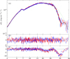 |
Fig. 7. a: X-ray spectrum of Vela X-1 as measured with NuSTAR (ObsID 30002007003). Data from the two instruments of NuSTAR, FPMA and FPMB, are shown in red and blue, respectively. The best-fit model as presented by Fürst et al. (2014) is shown in black. The dashed green lines indicates the continuum model without the CRSF components. b: residuals in terms of χ2 between the data and the best-fit model. c: residuals between the data and the model without the CRSF components. The harmonic line around 55 keV is much more prominent than the fundamental line around 25 keV. |
Earlier studies found no significant variation of the CRSF energy with flux. Fürst et al. (2014) found a positive correlation of the harmonic (higher-energy) line with flux, as expected for a source in the subcritical accretion regime as defined by Becker et al. (2012). La Parola et al. (2016) undertook a long-term study of Swift/BAT data of Vela X-1. While the fundamental line was not evident in their 15–150 keV spectra, the first harmonic of the CRSF was clearly detected between ∼53 and ∼58 keV, and with an apparent positive correlation of the line energy with luminosity, flattening above L1−150 keV ≈ 5 × 1036 erg s−1. Recently, Ji et al. (2019) reported a secular decrease of the energy of the harmonic line, again based on Swift/BAT data. If confirmed, this would indicate a slow change in the magnetic field configuration close to the polar caps.
One important caveat when results from different studies are compared is that different choices of mostly phenomenological spectral models for the continuum and for the cyclotron line parameters themselves lead to fit parameters that are intrinsically not directly comparable. Even the line centroids determining ECRSF, n (Eq. (7)) can be systematically different between different line models by a few keV for the same fitted spectrum, as explained in detail in Staubert et al. (2019, Sect. 3).
3.1.6. Pulse period variations
The long-term pulse period evolution of Vela X-1, reminded in Fig. 8, is usually described as a random walk. In an in-depth study of HEAO-1 data, Boynton et al. (1984) found that the power density spectrum covering timescales from 0.25 to 2600 days can be described by assuming white noise in angular acceleration, or equivalently, a random walk in pulse frequency. Short-term angular accelerations were found to be as large as  . According to their analysis, apparent changes in secular trends and frequency variations on shorter timescales of at least days are all consistent with the same random noise process in angular acceleration. This result was reinforced and refined in subsequent papers (Boynton et al. 1986; Deeter et al. 1989) and also by a similar study based on the Hakucho and Tenma satellites (Deeter et al. 1987a). de Kool & Anzer (1993) extended these studies by combining data from Nagase (1989) and Raubenheimer & Ögelman (1990), again confirming that the pulse period behavior is very well fit by a random walk. Boynton et al. (1984) also noted that the short-term angular accelerations reported in their study were much larger than expected for accretion from a uniform wind, assuming the wind speeds given in Dupree et al. (1980), and that the flow may form a ring or disk around the neutron star.
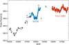 |
Fig. 8. Evolution of the pulse period of Vela X-1 as observed by diverse instruments (gray squares, see Table A.2 for details), by CGRO/BATSE (blue circles) or by Fermi/GBM (red circles). BATSE and GBM period determinations are derived over two and three intervals of the orbit, respectively. Note the scale. The longest reported pulse period differs by ∼0.3% from the shortest known pulse. |
3.1.7. Pulse profiles
The first observations discovering the periodic pulsations of Vela X-1 with the SAS-3 X-ray observatory have found a complex pulse profile structure with five visible peaks at energies below 6 keV and two broad peaks at the higher energies above ∼10 keV, which are both somewhat asymmetric, with a sharper trailing than leading edge (Rappaport & McClintock 1975; McClintock et al. 1976). The overall structure of the pulse profile has been confirmed in many subsequent studies of the system (e.g., Nagase et al. 1983; Raubenheimer 1990; Kreykenbohm et al. 1999; La Barbera et al. 2003), across significant variations in X-ray brightness. It can be considered a fingerprint of the X-ray pulsar, like in many other systems. In other words, while some variations in the observed profile are visible when different observations are compared, especially in the peak fluxes of different pulse components, the overall shape and thus the underlying emission geometry is evidently very stable. This is also demonstrated in Fig. 9. The main visible differences at the lower energies can be caused by the sometimes very strong absorption and scattering (Sect. 3.1.3), which can smear out especially the low-energy profile (Nagase et al. 1983). For detailed pulse profiles across a wide energy band, see especially Raubenheimer (1990, Fig. 1) and La Barbera et al. (2003, Figs. 1–4).
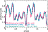 |
Fig. 9. Comparison of the complex low-energy pulse profile in the roughly 2–6 keV energy range from observations taken decades apart with three different X-ray missions, SAS-3, EXOSAT, and BeppoSAX, respectively. The data points have been taken from McClintock et al. (1976), Raubenheimer (1990), and La Barbera et al. (2003), but shifted in phase and scaled arbitrarily for a visual match. |
When different observations are compared, we recall that like in many other accreting X-ray pulsars, there are clear variations between individual pulses, as demonstrated in the first detailed study of the hard X-ray pulsations (Staubert et al. 1980) and later studies (Kendziorra et al. 1989; Kretschmar et al. 2014). These variations may affect the mean pulse profile of observations that cover only a limited number of pulse period intervals.
In earlier publications, pulsations were found to cease during off-states (Inoue et al. 1984; Kreykenbohm et al. 1999, 2008). Observations of off-states are summarized in Table 1. This behavior might be interpreted as the onset of the propeller regime (Sect. 2.3). In contrast, Doroshenko et al. (2011) analyzing three off-states observed with Suzaku, did observe remaining pulsations, but with significant changes in the pulse profile. They interpreted this behavior as gated accretion, with some remaining accretion.
Overview of off-states or low-flux observations of Vela X-1 reported in the literature.
A very peculiar observation was reported by Kretschmar et al. (2000): For a duration of several hours, the source flux diminished, but was still significantly above the background level, while pulsations ceased practically completely. After this low-state phase, there was a high state with strong, flaring pulsations, but a very similar spectrum to the preceding nonpulsating state. At the time, an explanation by a very thick clump in the wind was put forward, but in the light of newer results on wind properties and realistic clump sizes (see Sect. 2), this seems very unlikely.
Liao et al. (2020) reported another case of a low-flux state with ceasing pulsations. Based on spectral evidence, this was interpreted as formation of a (temporary) accretion disk in this case. We also note the explanation put forward by King & Lasota (2020) for suppressed pulsations in ultraluminous X-ray sources by scattering in a thick beaming funnel. This role would be played in Vela X-1 by the transient disk-like structure.
3.2. Optical, UV, and IR diagnostics
3.2.1. Photometric light curve
The study of photometric data, and in particular, the shape and amplitude of the optical light curve, is a tool that beyond determining the photometric period can be used through comparison with models to infer information on system parameters such as the size of the components relative to the orbit or the mass ratio. For a review, see Wilson (1994a); a visualization of a model light curve for Vela X-1 is included in Wilson (1994b). Several studies of this type have been performed in the 1970s and 1980s. All of them reported variability on the photometric light curve from one cycle to another. At later times, system parameters were instead obtained from X-ray studies, which allowed a more accurate determination of the system parameters.
The first photometric study of HD 77581 was carried out by Vidal et al. (1973) in the V band over a time span of 16 days. They observed four minima in the light curve that were consistent with the reported period of 8.95 ± 0.02 days by Forman et al. (1973). They reported a small amplitude of the light curve of ∼0.14 mag and found some evidence of variability with the period, particularly at the primary minimum. This behavior was attributed by Vidal et al. (1973) to the important role played by tidal effects.
The same periodicity was confirmed by Jones & Liller (1973) using UBV photometric observations of the companion over 27 consecutive nights, including two maxima and two minima. They reported an unexpected nonrepeatability of the optical light curve from cycle to cycle with color-free erratic changes. They explained this as due to complex changes in the upper layers of the star that are comparable to the gravity-darkening effect.
Petro & Hiltner (1974) combined the observations of Vidal et al. (1973) and Jones & Liller (1973) with three new campaigns to obtain a more precise determination of the photometric period of 8.972(1) days. They noted systematic deviations between the data and the best-fitting circular-orbit light curve, which might be explained by an elliptical orbit.
Vidal (1974) presented a more extensive set of observations in V band with 126 observations in total, including those reported in Vidal et al. (1973), which were obtained during the period of 22 January–19 June 1973. They reported that the most interesting feature of the light curve was the high scatter of the data throughout the whole period and claimed that this variability was intrinsic to the source. They observed that the rising and descending branches of the light curve during primary minimum were different and interpreted the shape of the light curve as due to different aspects of a tidally distorted companion.
Zuiderwijk et al. (1977a) presented a four-color photometric study of HD 77581 in the Strömgren uvby system. They observed the source on 46 nights in three campaigns in 1975. The magnitudes are listed in tabular form in Zuiderwijk et al. (1977b). These observations also showed changes in the light curve from one orbit to another. They found a regular wave-like variation in the color index c1 and possibly in b − y in phase with the light curves and twice noted the disappearance of a maximum during their observations, as also reported by Jones & Liller (1973). The observed variability in the light curve and the colors were interpreted with a model of a tidally distorted rotating primary.
van Genderen (1981) carried out a VBLUW photometric study in 1976 and 1977. They obtained a photometric period of 8.9615 ± 0.0025 days, which is closer to the contemporary measured period of the X-ray light curve. They reported the peculiarities of the mean light curve, which had a total amplitude of ∼0.10 mag, with a difference in height between the maximum and the minimum of ∼0.04 mag. The minimum seemed to be delayed by ∼0.1 in phase with respect to the center of the X-ray eclipse. The high peaked maximum varied in height and possibly in phase with a timescale of about two years. They concluded that the observed intrinsic variability of the light curve was correlated with the appearance and disappearance of hotter or cooler areas in the stellar atmosphere.
Khruzina & Cherepashchuk (1982) performed an analysis of all published photometry data and revealed a regular long period of 93.3 days of the optical light curve (B band). This period was later confirmed by Cherepashchuk (1982) using independent new UBV photometric data obtained at Siding Spring Observatory in February–June 1980. Khruzina & Cherepashchuk (1982) and Cherepashchuk (1982) associated this long-term period with forced precession of the rotation axis of the optical companion. This induces changes in the eclipsing gas streams and in the accretion structure. While super-orbital periods have been detected for other HMXBs (Corbet & Krimm 2013), no such periodicity has been reported for Vela X-1.
Tjemkes et al. (1986) developed a simple geometric model to analyze the optical light curves of several X-ray binaries and compared their predictions with real data (see Fig. 10). In the case of HD 77581, they used all published data in addition to data obtained in 1979 and 1980 to compute an average visual light curve. Ellipsoidal light variations were observed in the light curve, which is indicative of a donor star close to filling its Roche lobe. The light curve had two brightness maxima and two minima, and a photometric period of 8.965 ± 0.001 was reported. However, the light curve presented some particularities: (1) the two maxima are different in shape and brightness level, (2) the minimum is somewhat asymmetric and is shifted with respect to the mid-time of the X-ray eclipse by 0.05, and (3) the scatter around the average light curve is ∼0.02, which is much larger than the accuracy of the photometric data. These variations occurred on timescales from hours to many days. They carried out a search of the long-term period reported by Khruzina & Cherepashchuk (1982) and Cherepashchuk (1982) and detected some indications in favor of a minimum variance near 93.2 d, but no significant evidence to support the existence of this super-orbital period. Overall, Tjemkes et al. (1986) found serious discrepancies between their model and the data for the minima and concluded that the model did not describe the region near the inner Lagrangian point well. They suggested that basic model assumptions, in particular the instantaneous adjustment of the primary shape to the equipotential surface, are invalid for an eccentric orbit.
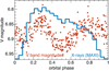 |
Fig. 10. V-band magnitudes of HD 77581 as compiled by Tjemkes et al. (1986, Fig. 8), demonstrating the intrinsic scatter, which is much larger than measurement uncertainties. For visual comparison, we plot the mean orbital profile in X-rays as observed by the MAXI instrument from Fig. 4 in the background. |
Wilson & Terrell (1994) fit optical light curves, optical velocities, and X-ray pulse arrival times simultaneously to reproduce the observed X-ray eclipse duration. They assumed a binary star model on equipotentials with an eccentric orbit and adjusted the varying tidal effect. The companion star rotated at a constant angular rate. They concluded that the optical star rotates subsynchronously and presents phase shifts that the authors interpreted as tidal lags. Both of these properties have major implications for understanding the scenario of the system evolution. According to Wilson & Terrell (1994), the system could be on the verge of a common evolution scenario.
3.2.2. Radial velocity curve
In an eclipsing X-ray binary system, the procedure for determining the neutron star mass is based on the radial velocity (RV, hereafter) curve of the companion star, as determined from shifts in the positions of various observed spectral lines, knowing the orbits of the two components, and knowing or assuming the inclination of the system. This procedure is valid under the assumption that RV curve variations truly represent the orbital motion of the star. In the case of HD 77581, this assumption is highly questionable for two reasons: the prominent line profile variability (van Paradijs et al. 1977a; van Kerkwijk et al. 1995; Barziv et al. 2001; Quaintrell et al. 2003), and the asymmetries over the orbital cycle of the RV curve (van Paradijs et al. 1977a; van Kerkwijk et al. 1995; Barziv et al. 2001).
The first RV study of HD 77581 was performed by Hiltner et al. (1972) using a Coudé spectrograph with a total of 85 spectrograms. They found variability on the source, and the velocity curve was not sufficiently defined to warrant a detailed analysis. They concluded that the system was a spectroscopic binary with a provisional period of 7 d and a minimum mass of the companion near 1.4 M⊙.
In 1974, several publications (Wickramasinghe et al. 1974; Mikkelsen & Wallerstein 1974; Zuiderwijk et al. 1974; Hutchings 1974) carried out an analysis of the RV curve. No consistent orbital elements could be derived, however, leading to estimates of the mass of the compact object that were too large to be consistent with those of a neutron star.
van Paradijs et al. (1976) performed the first relatively accurate determination of masses for both partners using RV measurements. They used 26 Coudé spectrograms to determine the total mass of the system as well as the masses of each component. In contrast to previous work, they excluded the lines of hydrogen because they are the most affected by gas motions in the system. Using He I lines and lines of heavier ions, they derived mean values of the RV for all the lines and for the He I and heavier-ion lines independently. They obtained a semiamplitude of the RV curve of Kopt = 20 ± 1 km s−1 and derived a total mass of the system of ∼21.6 M⊙, with a mass of the compact object of ∼1.6 M⊙, and ∼20 M⊙ for the companion (see Table 4).
van Paradijs et al. (1977a) carried out a more detailed optical RV study to improve the accuracy of previous works and to investigate the possible presence of the distortion effect predicted in van Paradijs et al. (1977b). They found short-term autocorrelated nonorbital variations, but because so many factors were involved, they were unable to estimate the amplitude of the individual nonorbital contributions. They derived a more accurate Kopt = 21.75 ± 1.15 km s−1 than in van Paradijs et al. (1976) and claimed that the mass of the primary was rather low for its spectral type and luminosity class (see Table 4), a similar type of undermassiveness as was found for SK 160 in SMC X-1.
Nearly 20 years later, van Kerkwijk et al. (1995) performed a RV curve analysis using optical and IUE data. Since the previous mass determination, the statistical and systematic accuracy of stellar spectroscopy had improved significantly following the introduction of CCDs detectors. Thus, they expected to obtain a smaller error on the RV determination. However, this was hampered by the large deviations from a pure Keplerian RV curve. As did Hiltner et al. (1972), Zuiderwijk et al. (1974), van Paradijs et al. (1977a), they reported velocity differences with respect to the orbital fit dominated by random excursions that they found to be autocorrelated within one night, but not from night to night. They found substantial and very similar changes in the shape of the profiles of all the lines. These changes in the lines plus the velocity variability were interpreted as due to large-scale motion of the surface induced by tidal forces due to the presence of the neutron star. This is the same underlying physical mechanism that Tjemkes et al. (1986) proposed to explain the irregular variations of the optical light curve. van Kerkwijk et al. (1995) derived a Kopt = 18.0−28.2 km s−1 (95% confidence range) and concluded that the accuracy of the RV study is limited by three factors: (i) the velocity excursions, (ii) possible effects induced by the tidal deformation, and (iii) the possible presence of systematic positive deviations in velocity close to the time of minimum velocity. To derive more accurate constraints on the orbital parameters, they suggested that the short- and long-term behavior of the system should be studied to better understand the tidal interaction.
For a better understanding of the radial-velocity excursions, Barziv et al. (2001) performed an extensive long-term spectroscopic campaign for about nine months following one of the recommendations given by van Kerkwijk et al. (1995). They expected that the velocity excursions would average, thus allowing a more accurate determination of the RV amplitude than previous works. They determined the RV from several lines using the same cross-correlation algorithm as van Kerkwijk et al. (1995). As in previous analyses, they found strong deviations in the RVs from those expected for a pure Keplerian orbit, with root-mean-square amplitudes of ∼7 km s−1 for strong lines of Si IV and N III near 4100 Å, and up to ∼20 km s−1 for weaker lines of N II and Al III near 5700 Å. They found that systematic deviations depended on the orbital phase, with the largest deviations observed near inferior conjunction of the neutron star and near the phase of maximum approaching velocity. They also reported a so-called blue excursion in the Hδ data and interpreted it as a photoionization wake. They inferred a radial-velocity amplitude Kopt = 21.7 ± 1.6 km s−1 with an uncertainty not much smaller than was found in previous analyses, in which the effect of systematic phase-locked deviations were not taken into account.
To overcome the velocity excursions issue, Quaintrell et al. (2003) carried out a comprehensive RV study with maximum phase coverage over two consecutive orbits of the system instead of averaging the velocity excursions over many orbital periods. They found evidence for tidally induced nonradial oscillations from the power spectrum of the residuals to the RV curve fit. Moreover, when they allowed the zero phase of the RV curve to vary instead of constraining it to the X-ray ephemeris, the fit significantly improved and they obtained a semiamplitude of the RV curve of Kopt = 21.2 ± 0.7 km s−1. This is the most accurate value to date (see Table 4 for a comparison of the determined Kopt). Quaintrell et al. (2003) concluded that this apparent shift in the zero-phase may indicate an additional RV component at the orbital period, which could be another manifestation of the tidally induced nonradial oscillations and an additional source of uncertainty in RV studies.
Koenigsberger et al. (2012) have explored the manner in which surface motions induced by the tidal coupling between the blue supergiant and the neutron star affect the RV curve (for the theory of tides in general, see Zahn 1989). They developed a 2D code that provides the time-dependent shape of the stellar surface and its surface velocity field for the general case of an elliptic orbit and asynchronous rotation without considering the effects of a nonuniform temperature distribution over the stellar surface. They concluded that the tidal effects on the RV curve produce orbital phase-dependent variations in the profiles that lead to asymmetries, blue or red wings. Moreover, the line-profile variability induces a significant variation from a Keplerian RV curve that artificially enhances the semiamplitude. One point of note is that a prominent feature appears in their synthetic RV curves: A blue dip occurs shortly after the maximum. This is caused by the asymmetrical shape of the line profiles. This feature coincides with the blue excursion reported by Barziv et al. (2001), and it could be explained by a higher mass outflow after periastron passage, where the tidal effects are stronger.
3.2.3. Quantitative spectroscopy
The stellar and wind parameters of hot massive stars such as HD 77581 are frequently determined through quantitative spectroscopy, that is, by fitting synthetic spectral energy distributions and normalized spectra to observations, mainly optical and UV spectra. The best-fitting spectra and thus parameters are frequently found by eye in a visual comparison of models and data or by minimization on a grid of spectra.
The main parameters derived in these studies are the measured color excess (EB − V), the (effective) stellar temperature (T⋆) from the ionization equilibrium determined from line ratios, the surface gravity (g⋆), and the projected rotational velocity (vrot sin i). Stellar radii and thus luminosities are then derived using the temperature, absolute magnitude (depending on the assumed or derived distance), and the bolometric correction. An overview of methods and diagnostics used for these studies and caveats to consider are given in Martínez-Núñez et al. (2017).
Early studies in the 1980s were undertaken before codes that describe hot stellar atmospheres were developed. These studies relied on an examination of specific lines and a comparison to similar stars. Dupree et al. (1980) carried out a simultaneous observation program in the X-ray, ultraviolet the International Ultraviolet Explorer satellite (IUE), and optical bands. They mainly used the comparison of P Cygni lines with the atlas of Castor & Lamers (1979) and theoretical profiles provided by Olson (priv. comm. of Dupree et al. 1980) to estimate the terminal velocity and mass-loss rate of the line-driven wind. Sadakane et al. (1985) analyzed IUE spectra of HD 77581 by comparing individual lines with the corresponding lines from well-studied single B0-B1 supergiants. Other examples in which specific line features were used to estimate some stellar wind or line properties include Prinja et al. (1990) for terminal velocities of massive star winds or Zuiderwijk (1995) for the rotation period and rotation velocity of HD 77581.
From the 1990s onward, nonlocal thermodynamic equilibrium (NLTE) hydrostatic codes began to be used to genereate synthetic spectra. In a seminal paper, Vanbeveren et al. (1993) used a plane-parallel code by D. Kunze for the comparison with optical spectra with high signal-to-noise ratio in the range 4175–4525 Å to derive stellar parameters. Using the orbital parameters of Rappaport & Joss (1983), they determined a range of stellar parameters satisfying the orbital, X-ray eclipse, and stellar atmosphere analysis.
The NLTE codes SYNSPEC2 (Hubeny et al. 1985) and TLUSTY3 (Hubeny & Lanz 1995) were used by Fraser et al. (2010) to calculate model atmosphere grids. These were then compared with high-resolution (R ∼ 48 000) spectra obtained with the Fiber-fed Extended Range Optical Spectrograph (FEROS)4 for very many massive stars, including HD 77581, in order to determine the atmospheric parameters (effective temperature, surface gravity, and microturbulent velocity), the surface nitrogen abundances, and the rotational and macroturbulent velocities. These codes do not take the inhomogeneities of the wind into account, however, and are optimized for hot stars with no significant wind.
A stellar wind can considerably alter the spectral appearance and for example spoil the derived stellar parameters such as log g if it is not taken into account. So-called unified model atmospheres are necessary to consistently describe the outermost layers of the star and their winds. Model atmospheres like this are inherently in NLTE and have considerably improved over the past decades through higher computational power and the better understanding of physical processes in stellar atmospheres (Sander 2017), for example, by properly accounting for the complex effects of the millions of iron lines. While modern codes provide a more accurate determination of the stellar and wind parameters, a proper comparison of observed and model spectra can only be automatized to a certain degree (see also Martínez-Núñez et al. 2017). In any case, spectral analysis studies should be performed using as many lines as possible because a particular single line can be affected by a variety of parameters, and it requires detailed knowledge about which features are affected by which parameters.
Giménez-García et al. (2016) carried out the first detailed study of HD 77581 using models with an expanding stellar atmosphere for line-driven winds generated by the Potsdam Wolf-Rayet (PoWR)5 model atmosphere code (Gräfener et al. 2002; Hamann & Gräfener 2003). The PoWR code takes line-driven winds, wind clumping, and a plethora of ions into account. These were compared to the previously mentioned IUE and FEROS spectra to derive stellar and wind parameters. The rotational velocity, the β exponent for the wind velocity profile (Eq. (1)), and the macroturbulence were set based on insights from previous works and on spectral line shapes and depths. They also found indications of chemical evolution in the star, with a moderate overabundance of He and N, together with an underabundance of C and O.
In recent years, the PoWR code has been extended with the option to consistently solve the hydrodynamic and statistical equations in 1D, together with the radiative transfer, in order to obtain a hydrodynamically consistent atmosphere stratification (Sander et al. 2017). This was applied to the Vela X-1 system in Sander et al. (2018), who in a simplified manner also included the effect of the X-ray radiation (see also Sect. 4.1.2).
Tables 5 and 7 in Sect. 5.6 give an overview of the parameters that were derived mainly from quantitative spectroscopy. In some cases, these results were also used to infer information about other properties of the system (see Sects. 5.1 or 5.3 and Table 4).
3.2.4. UV resonance lines
Hatchett & McCray (1977) predicted that an X-ray source in the stellar wind of an early star produces changes in the photospheric ultraviolet resonance lines of ions such as Si IV, C IV, Al III, or N V. They also predicted that the lines vary along the orbit and that these variations can be used to determine the size of the stellar wind region that is affected by the X-ray ionization induced by the compact object. However, the amplitude of the observed orbital modulation also depends on the density and velocity of the stellar wind.
Dupree et al. (1980) presented the first UV resonance line study of the system using IUE observations. They detected very prominent P Cygni profiles in the resonance lines of Si IV (1393.75 Å and 1402.77 Å) and C IV (1548.19 Å and 1550.76 Å). They observed variability in the profiles over the orbital phase with more dramatic changes in the Si IV than in the C IV profiles. They reported that when the compact object is in front of the mass donor, around orbital phase 0.5, the P Cygni absorption is ionized to a higher state than at eclipse, and the emission component is increased. They concluded that the observed variability and the variation in the edge velocity could be qualitatively explained by the Hatchett–McCray effect (hereafter, the HM effect).
Sadakane et al. (1985) detected P Cygni profiles of the C IV and Si IV resonance lines in the same way as Dupree et al. (1980), and in addition, they reported the Al III resonance doublet at 1854.72 Å and 1862.79 Å. They found similar profiles and variations on the C IV and Si IV as Dupree et al. (1980). In the case of Al III, they found a remarkable difference in the profiles before and after mid-eclipse. They explained this behavior as due to the complex structure of the stellar wind with two different components, the high- and low-velocity components. The low-velocity component seemed to be present only from mid-eclipse and during the second half of the orbital cycle. They claimed that it was formed near the secondary and that its origin might be a trailing wake behind the compact object. On the other hand, the high-velocity component was observed throuhgout the orbit and was interpreted as originating from a cooler expanding region.
Kaper et al. (1993) carried out a study to investigate the dynamical structure of the stellar wind in the system using IUE data. They also observed orbital variations in the blueshifted absorption part in the Si IV and C IV resonance lines. When the compact object was in front of the optical companion, the Si IV absorption was weaker not only at high velocities (∼−700 to −1300 km s−1) as reported by Dupree et al. (1980), but also at low velocities (∼−300 to −500 km s−1). In the case of C IV, they found variations at high velocities, whereas at low velocity, the variations were not significant. Like Sadakane et al. (1985), they also found variations in the Al III resonance, but in this case, also at low and intermediate velocities. They interpreted the larger Al III variations as due to ionization effects. In addition, they reported N V resonance lines at 1238 and 1242 Å for the first time, with variations in the absorption part that are consistent with the changes found in the Si IV and C IV profiles and consistent with the variability predicted by the HM effect. Regarding the emission of the P Cygni lines, Kaper et al. (1993) found stronger emission in the Si IV, C IV, and Al III profiles around the mid-eclipse phase when the X-ray source is in the line of sight. They estimated that these orbital variations of the redshifted emission extended to about 1000 km s−1 for the Si IV and C IV lines. The N V resonance doublet showed different variability at the short- and in long-wavelength sides. In the former, the strongest emission was observed during eclipse, and in the latter, the red emission peak is remarkably stable throughout the orbit. In conclusion, Kaper et al. (1993) reported an orbital modulation of the P Cygni profiles not only in the high-velocity part of the profiles, but also at intermediate and low velocities. This shows the occurrence of the HM effect for the full range of velocities. Their observations could not be explained with a monotonic stellar wind combined with partial ionization. They concluded that the resonance lines can be better understood if in some regions, the wind decelerates, in agreement with the predictions from hydrodynamical calculation of radiation driven winds performed by Owocki et al. (1988).
van Loon et al. (2001) presented the first quantitative analysis of the UV spectral variability in five HMXBs including HD 77581, for which they used high-resolution spectroscopy obtained with the IUE satellite. Their synthetic profiles were obtained using a modified version of the Sobolev exact integration method of Lamers et al. (1987), including a nonmonotonic wind structure, turbulence, and an extended X-ray photoionized zone. The line profiles of Si IV, C IV, and Al III and their orbital modulation were rather well reproduced by their model, with an additional absorption component due to a photoionization wake that was previously indicated by Kaper et al. (1994) using strong optical lines such as the hydrogen Balmer lines and He lines. In the case of the N V resonance line, their model was unable to properly reproduce the profile, and it seemed that this line was more affected by the photoionization wake than the other lines. From these data, they were able to derive the extent of the region in which line-acceleration is quenched because the energy levels that are most strongly responsible for it are depopulated by the X-ray photoionizing feedback.
3.2.5. Infrared diagnostics
Observations of Vela X-1 beyond the near-infrared region of the spectrum have been reported only rarely. Smith et al. (1990) listed HD 77581 with significant Infrared Astronomical Satellite (IRAS) fluxes in their collection of 81 X-ray binary counterparts, but did not discuss this further in their study, which focused on infrared emission from accretion disks. Friedemann et al. (1996) noted that the IRAS fluxes reveal cold dust and that the binary may be surrounded by a fossil dust shell.
As detailed in Sect. 5.1.2, Vela X-1 is associated with a wind bow shock in the interstellar medium. This structure was first discovered in a Hα image (Kaper et al. 1997), but has been studied in the infrared based on IRAS (Huthoff & Kaper 2002), Spitzer (Gvaramadze et al. 2011), and WISE (Maíz Apellániz et al. 2018) observations.
Choquet et al. (2014) obtained infrared interferometric observations of Vela X-1 with the VLTI in the K band (2.2 μm) in 2010 and in the H band (1.6 μm) in 2012. The second observations covered different orbital phases (0.89, 0.11, 0.33, and 0.55), but with no significant variation in the interferometric observables. In the K band, a structure of 8 ± 3R⋆ was resolved, while two years later, a centro-symmetric structure of radius  was found in the H band. The authors offered three different possible explanations for the difference in derived diameters: (1) A strong temperature gradient in the supergiant wind, where hot material at 1720 K is more compact than material at 1350 K; (2) a diffuse gaseous shell observed in 2010, which had diffused two years later; or (3) the structure observed in the H band was the stellar photosphere and not the supergiant wind.
The chemical evolution noted for HD 77581 could indicate that shock chemistry may be dominant in the surrounding interstellar medium. For other regions of the sky, it has been shown that relevant dynamical and physical parameters of the shocked gas can be determined by analysing its far-infrared (far-IR) emission lines (e.g. Lerate et al. 2008). In the same vein, the study of far-infrared emission lines could provide a better insight into the wind clumps and structure.
The region of Vela X-1 has been briefly observed by Herschel in 2012, but no associated publications are found in the Herschel Science Archive.
3.3. Radio observations
On 15 May, 2018, van den Eijnden et al. (in prep.) observed Vela X-1 with the Australia Telescope Compact Array. This four-hour observation yielded the first radio detection of the source at flux densities of 92 ± 11 and 122 ± 10 μJy at 5.5 and 9 GHz, respectively. These measured flux densities imply a spectral index measurement of α = 0.56 ± 0.36, where Sν ∝ να. The observation was performed completely during the eclipse of the neutron star, at orbital phases of 0.92–0.94.
With the currently known radio properties of Vela X-1, it is challenging to determine the dominant radio emission process. While in LMXBs radio emission has been established as a signature of synchrotron-emitting jets (except for the handful of LMXBs hosting a strongly magnetized neutron star), the massive donor and its wind in HMXBs can also contribute to the observed radio emission. The properties of Vela X-1 fit both scenarios: The spectral index is consistent with that of a steady, compact jet, as seen typically in hard states of persistent low-mass X-ray binaries (α = 0–0.7; Fender et al. 2004). The radio luminosity of Vela X-1, interpolated to be ∼2 × 1027 erg s−1 at 6 GHz, is also similar to the radio emission of other jets launched by strongly magnetized (e.g., B > 1012 G) accreting neutron stars (van den Eijnden et al. 2018a,b,c, 2019). Similarly, the spectral index fits the predicted spectral index for thermal radio emission from an ionized stellar wind (α = 0.6; Wright & Barlow 1975; Güdel 2002). The flux densities also fit within their uncertainties the predicted brightness of such a wind following the formalism in Wright & Barlow (1975), assuming a mass-loss rate of 10−6 M⊙ yr−1 and a terminal wind velocity of ∼700 km s−1 (Grinberg et al. 2017).
Both scenarios could have significant implications: First, strongly magnetized neutron stars were long thought to be incapable of launching jets (e.g., Fender & Hendry 2000; Migliari & Fender 2006; Massi & Kaufman Bernadó 2008), until the recent detection of such a jet showed otherwise (van den Eijnden et al. 2018c). If Vela X-1 also launches a jet, it would add to the still small but growing sample of strongly magnetized neutron stars launching jets (van den Eijnden et al., in prep.). Alternatively, if a wind is observed in radio, it would only be the second HMXB with a radio wind detection (after GX 301−2; Pestalozzi et al. 2009). Based on its high inclination and clear orbital variation of the wind absorption, Vela X-1 would provide a unique and powerful testbed in which to explore the properties of stellar winds in HMXBs in radio, while at the same time, radio observations would provide a new and complementary view of Vela X-1 itself.
At the time of writing, however, the first challenge is to probe the origin of the detected radio emission: jet, wind, or a combination of both? Detailed radio and X-ray monitoring over several orbital phases will be vital for this purpose, revealing the variability of the radio properties and allowing a comparison between accretion, X-ray, wind, and radio properties along the orbit.
4. Models of Vela X-1
Like most wind-fed HMXBs, Vela X-1 is a system that can only be appreciated with multiphysics and multiscale models (see Fig. 2). Many efforts have been made to capture the predominant mechanisms at each scale. In simplified geometries assuming an isotropic stellar wind (1D models) or focusing on the orbital plane (2D models), some semianalytic results were derived. However, since the late 1980s, numerical simulations have been the privileged tool for capturing the whole 3D complexity of this archetypical system and provide suitable models for interpreting the observations.
4.1. Stellar wind
4.1.1. Hydrodynamic structure
The donor star is not isolated in Vela X-1. The presence of the orbiting neutron star breaks the spherical symmetry of the problem, and the wind cannot be fully described in a 1D framework. If the wind speed were much higher than the orbital speed, the wind would only be affected by the gravitational field of the neutron star in a region far smaller than the orbital separation (see the discussion of the accretion radius in Sect. 4.2). Except in the thin wake of the accretor, which is axisymmetric with respect to the axis joining the two bodies, the 1D representation would hold. On this implicit assumption Watanabe et al. (2006) relied when they empirically introduced a cone-shaped dense and cold cloud in the wake of the neutron star to explain the excess of absorption at inferior conjunction. In the same spirit, Fryxell et al. (1987) performed wind tunnel simulations: They ran 2D axisymmetric hydrodynamic simulations on a spherical grid of a planar adiabatic flow coming from infinity with a supersonic relative speed that was deflected by the gravitational field of an accretor. This configuration corresponds to the problem that was first addressed by Hoyle & Lyttleton (1939) and Bondi & Hoyle (1944) in ballistic terms, the BHL configuration. Fryxell et al. (1987) found a good agreement with the BHL predictions and that an axisymmetric bow shock forms around the accretor, with an opening angle depending on the Mach number of the flow. Provided the orbital effects are negligible, that is, when the wind speed is much higher than the orbital speed, the flow in a wind-fed HMXB can be divided into two parts: A purely radial wind flowing away from the donor star, and in the immediate vicinity and in the wake of the compact object, a flow that is well described by the BHL solution or by its hydrodynamics counterpart.
Nevertheless, in Vela X-1, a more realistic wind speed at the orbital separation of about or even lower than the orbital speed, such as the one used by Watanabe et al. (2006) and Sander et al. (2018) (see Sect. 4.1.2), indicates an anisotropic wind that surrounds the donor star. The outflow is strongly shaped by the orbital motion, as is corroborated by the systematic asymmetries observed in the absorbing column density profile6 between orbital phases 0–0.5 and 0.5–1 (see Sect. 3.1.3). In this case, a fully 3D model is required to describe the hydrodynamic structure of the wind and interpret the evolution of the observations with the orbital phase in a high-inclination HMXB such as Vela X-1. Bessell et al. (1975) first highlighted the anisotropic distribution of material in the orbital plane induced by the tidal forces. It was later confirmed by 2D hydrodynamic simulations in the equatorial plane of a spherical mesh by Blondin et al. (1990, 1991). They characterized the gravitational and radiative impacts of the neutron star on the wind: They showed that the nonsteady and overdense envelope of the bow shock that is formed upstream trails the neutron star throughout its orbit. This structure is referred to as the accretion wake. Blondin et al. (1991) further showed that in simulations of Vela X-1, the wind was highly focused into a steady tidal stream between the star and the neutron star. This feature is clearly visible in the 2D simulations by Manousakis et al. (2012). On the other hand, wind tunnel simulations centered on the neutron star but with a nonplanar inflow were previously performed on 2D cylindrical (r, ϕ) grids (Taam & Fryxell 1988, 1989; Fryxell & Taam 1988). The aim was to parameterize the shearing in velocity and/or mass density of the inflow that is caused by the orbital effects. They identified an oscillation of the accretion wake around the main axis of the cylinder, which they called the flip-flop instability (see also Matsuda et al. 1987, 1991, for the seminal simulations in which this effect was determined). First thought to be responsible for the formation of transient disks in wind-fed HMXBs, this feature was later found to be a numerical artifact due to the unrealistic geometry of the mesh and to the unphysically large size of the sink particle standing for the accretor (Ishii et al. 1993; Ruffert 1999; Blondin & Raymer 2012). In addition to the tidal stream and the accretion wake, a spiral-shaped density enhancement is to be expected at the side of the star opposite to the neutron star due to the tidal forces (El Mellah et al. 2019b). With the 3D framework they worked with, these authors also solved the dynamics of the wind off the orbital plane and found a significant flattening of the wind in the orbital plane when the ratio of the wind speed to the orbital speed was similar to what is expected for Vela X-1.
In Vela X-1, the microstructure of the wind is still poorly constrained, although Giménez-García et al. (2016) measured a density contrast in the wind that is consistent with theoretical predictions. Observational diagnostics that depend quadratically on density (e.g., Hα line and thermal radio emission) lead to overestimated mass-loss rates when clumping is not accounted for Sundqvist et al. (2012). Conversely, the mass-loss rates deduced from diagnostics that depend linearly on density (e.g., UV resonance lines) can be underestimated (Sundqvist & Puls 2018). Therefore the current uncertainties on the clumping factor prevent us from drawing a definitive conclusion concerning the stellar mass-loss rate. In Vela X-1, the size of the clumps derived from simulations and from the two main observational diagnostics at our disposal, absorption variability and X-ray flares, differs. While the first is thought to be due to unaccreted clumps passing the line of sight (see, e.g., the observations and model by Grinberg et al. 2017; El Mellah et al. 2020b, respectively), the second have been proposed to be due to the serendipitous capture of a clump by the neutron star (Fürst et al. 2010; Martínez-Núñez et al. 2014). However, hydrodynamics simulations by El Mellah et al. (2018) showed that the bow shock around the accretor significantly lowers the variability compared to a purely ballistic model of the clump capture. It suggested that although intrinsic X-ray flares might be triggered by clump capture, the amount of mass involved in a flare was probably much more important than the amount of mass contained in a single clump. A better understanding of the whole accretion process, from the orbital scale all the way down the accretion columns where most of the X-rays we observe originate, is necessary to determine the connection between the flares and the clumpiness of the wind.
4.1.2. Ionization structure and inhibition of wind acceleration
It is commonly accepted that the X-ray irradiation from the neutron star significantly affects the wind velocity profile, but it has proven very challenging to quantify the extent of this effect on the dynamics of the flow. In a seminal paper, Fransson & Fabian (1980) described how the photoionization of the wind by the accretor in high-mass X-ray binaries could lead to the formation of a shock between the accelerating wind and the stalling photoionized plasma. Blondin et al. (1990) quantified this effect with 2D numerical simulations. They modeled the effect of the X-ray ionizing feedback on the hydrodynamic structure of the wind. Assuming that wind acceleration was unaltered below ξcrit = 102.5 erg cm s−1 and fully inhibited above, they showed that the wind speed in the direction of the neutron star was lowered by a factor of ∼2. Because of the stalling of the line-driven wind that is caused by X-ray photoionization, in some simulations, the wind formed a trailing spiral density enhancement between the neutron star and the star. Kaper et al. (1994) relied on this photoionization wake to interpret an absorption component that they were unable to attribute to the accretion wake or to the tidal stream.
Although wind acceleration is inhibited in the limit case of a high X-ray illumination, for intermediate fluxes, it is not a step function nor even a monotonous dependence of the X-ray luminosity. For instance, as already noted by MacGregor & Vitello (1982), for intermediate X-ray photoionizing fluxes, the wind would overall be more efficient at absorbing UV photons, and the line-driven acceleration would even become higher. In Vela X-1, a few studies initiated by Sako et al. (1999), went beyond the on/off switch assumption in different ways. In a preliminary approach, Watanabe et al. (2006) assumed simplified descriptions of the line acceleration, the radiative transfer, and the ionization structure to compute 1D velocity profiles. They found a wind speed at the orbital separation in Vela X-1 of 180 km s−1 for LX = 3.5 × 1036 erg s−1 instead of 570 km s−1 without X-ray ionizing feedback. However, they did not iterate the radiative transfer and computation of the ionization structure and only accounted for a very limited number of line transitions.
More advanced treatments have emerged in the past decade to determine the effect X-rays have on the wind acceleration. In these methods, realistic stellar atmosphere models accounting for the inherent NLTE conditions and the moving outer layers were irradiated by an external X-ray source in order to study the imprint of the different elements and ions on the line acceleration. Krtička et al. (2012) derived wind solutions with the METUJE code (Krtička & Kubát 2017) for different axis in the orbital plane and iterated the radiative transfer and statistical equilibrium equations to obtain a consistent wind ionization structure. In a follow-up study, Krtička et al. (2018) accounted for optically thin wind clumping and obtained similar and very low values of the critical ionization parameter, above which line-acceleration was significantly inhibited, ranging between 5 and 25 erg cm s−1. In both cases, they computed wind velocities that were severely lower in the direction of the neutron star in Vela X-1, with a speed that hardly peaked at 100 km s−1. Following a spectral analysis by Giménez-García et al. (2016) that yielded updated parameters for the donor star and wind in Vela X-1, Sander et al. (2018) performed an analysis with the dynamically consistent branch of the PoWR code (Sander et al. 2017) to study the effect of X-ray irradiation on individual driving contributions and spectral lines. They showed that with the updated parameters, an X-ray ionizing source even as high as 1037 erg s−1 does not necessarily inhibit wind acceleration, but might even enhance it upstream the neutron star. While both METUJE and PoWR perform calculations in 1D, their results demonstrate that the wind speed could be so low that the outflow significantly departs from a spherically symmetric wind. However, the computational cost of these methods precludes any 3D direct computation in the next years.
Finally, it is worth mentioning that a preliminary global model of the radiation-driven photoionized wind was sketched and applied to Vela X-1 in Mauche et al. (2007, 2008). The authors combined different numerical tools. First, 2D and 3D hydrodynamical simulations were performed with FLASH (Fryxell et al. 2000). Second, the wind ionization structure was computed with the photoionization code XSTAR in order to derive the local heating and cooling rate, along with the ionization fractions of the different ions (Kallman & Bautista 2001). Third, the rich HULLAC database provided the emission models for the X-ray photoionized plasma (Bar-Shalom et al. 2001). Finally, a Monte Carlo radiative transport computation enabled them to derive detailed synthetic X-ray spectra.
4.2. Accreted flow
In Vela X-1, the ionization state and thus the whole hydrodynamic structure of the flow depends on the intensity of the X-ray emission from the neutron star, fed by the wind it illuminates. It emphasizes the need addressed by various authors for simultaneously modeling the orbital scale and the accretion process itself in order to achieve a fully consistent model that can connect the X-ray luminosity to the mass accretion rate. The accretion of stellar material by the neutron star proceeds in different steps. A mass transfer mechanism must first ensure that stellar material is brought into the Roche lobe of the neutron star if the flow has a negligible amount of specific kinetic energy, or is within the accretion radius given by Eq. (3) otherwise. These two characteristic length scales far exceed the other relevant scales of accretion, therefore we can first treat the mass transfer alone (Sect. 4.2.1). Then, accretion can proceed onto the magnetosphere of the neutron star and eventually carry the plasma all the way down the X-ray emitting regions near the magnetic poles (Sect. 4.2.2).
4.2.1. Mass transfer mechanisms
The donor star in Vela X-1 is unlikely to undergo RLOF. In X-ray binaries, mass transfer through RLOF usually leads to higher X-ray luminosities than in Vela X-1. Moreover, RLOF leads to the formation of a permanent accretion disk, which has not been observed in Vela X-1. The torques by such a disk would also spin the neutron star up, as is the case in Be X-ray binaries, but this contradicts the measured long neutron star spin period. An additional strong argument against mass transfer through RLOF comes from the stable orbital period (Falanga et al. 2015) because no outflow from the vicinity of the neutron star is observed and conservative mass transfer from a high-mass star to a low-mass accretor would lead to a quickly shrinking orbit (Quast et al. 2019; El Mellah et al. 2020a). Instead, accretion of the stellar wind is to be preferred as the dominant mass transfer mechanism.
Wind accretion as described by the BHL formalism might be a misleading alternative, however. Equation (4) has been widely used to interpret the intrinsic X-ray luminosity of Vela X-1 and its variations, but fundamental caveats must be acknowledged, especially because the wind speed at the orbital separation is not high compared to the orbital speed. It is plausible that a hybrid mass transfer mechanism is taking place in Vela X-1 (called wind-RLOF and introduced by Mohamed & Podsiadlowski 2007), where the wind is significantly disrupted and the geometry of the problem no longer obeys that of the planar BHL (see Sect. 2.1). For instance, the wind is compressed in the orbital plane by the motion of the two bodies, so that the density in Eq. (4) cannot be deduced from the continuity equation in spherical geometry. An approach to obtain more accurate mass transfer rates was introduced by El Mellah & Casse (2017), who assumed a donor star in synchronous rotation with the orbit and applied their model to Vela X-1: Because the wind is highly supersonic, ballistic streamlines reveal how beamed the flow is toward the neutron star, and density-enhanced (depleted) regions are identified where the streamlines diverge slower (faster) than in the spherically geometric case. The streamlines that intercept within the Roche lobe of the neutron star indicate the fraction of the stellar wind that will take part in the accretion process. They also enable us to compute the net specific angular momentum of the flow, which significantly departs from zero: An even more important reason to avoid the use of Eq. (4) in Vela X-1 is indeed that the flow might carry enough angular momentum to circularize before it reaches the neutron star magnetosphere, in contrast to the intrinsic assumption of cancelling angular momenta in the BHL picture.
The fact that the donor star does not fill its Roche lobe sets a stringent constraint on the orbital inclination angle i. If the eclipse duration relative to the orbital period is Δt/P, the ratio of the stellar radius R to the orbital separation a reads
where for now, we neglect the eccentricity of the orbit and the tidal deformations of the star. The condition of absence of RLOF yields a lower limit on the inclination angle,
![$$ \begin{aligned} i>i_{\mathrm{min}}=\arcsin \left[\frac{\sqrt{1-\mathcal{E} ^2(q)}}{\cos \left(\pi {\Delta t}/{P}\right)}\right] , \end{aligned} $$](/articles/aa/full_html/2021/08/aa40272-20/aa40272-20-eq12.gif)
where ℰ is the estimate of the ratio of the stellar Roche-lobe radius to the orbital separation provided by Eggleton (1983) and function of the mass ratio alone. For a given range of q and Δt/P, we can thus deduce a range of minimum orbital inclination angles below which the donor star would overflow its Roche lobe. In the upper panel in Fig. 11, we plot the minimum orbital inclination angle to avoid RLOF as a function of the mass ratio for realistic eclipse durations. At low mass ratios and for long eclipse durations (q < 12 and Δt/P > 0.2), the donor star would fill its Roche lobe even if the system were seen edge-on. Currently, the upper limit set on the eclipse duration is closer to Δt/P = 0.19 (Kreykenbohm et al. 2008), which would indicate a lower limit for the orbital inclination of ∼74°. This conclusion must be tempered, however, because the orbit is not circular. Moreover, the proximity of the donor star to filling its Roche lobe means that the star should not be assumed to be spherical, and only an effective stellar radius can be defined.
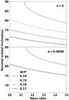 |
Fig. 11. Minimum inclination angle of the orbit for avoiding RLOF as a function of the mass ratio and for different durations of the eclipse relative to the orbital period. In the upper panel, a circular orbit is assumed, and in the lower panel, we account for an eccentricity of 0.0898 and enforce no RLOF even at periastron. |
Furthermore, the eccentricity of the orbit in Vela X-1 leads to a filling factor that varies with the orbital phase: Because the orbit is eccentric, the orbital separation varies, and so does the filling factor. When we enforce the more severe constraint to avoid RLOF even at periastron, we obtain the minimum inclination angles displayed in the lower panel in Fig. 11, which are significantly higher. Two conclusions can be drawn from this result. Either the system presents an orbital inclination and a mass ratio that lie at the upper edge of the intervals derived from observational diagnostics not based on the assumption of the absence of RLOF, or there are regular episodes of intermittent RLOF at periastron. In Fig. 12 we show the evolution of the Roche-lobe filling factor of the donor star as a function of the orbital phase for three different sets of system parameters derived from observations by Quaintrell et al. (2003), Rawls et al. (2011), and Falanga et al. (2015). At a given orbital phase, the uncertainty ranges are upper limits, obtained by considering the extreme values obtained without accounting for the correlations between parameters. The striking result is that observationally derived parameters tend to give filling factors above 1. When we take the absence of RLOF for granted, it means that we can set stronger constrains on the system parameters. With an eccentricity of 0.0898, however, the filling factor necessarily varies by ∼15% throughout the orbit. This major variation implies a mass transfer mechanism that might be modulated throughout the orbit, with a short phase of mass transfer through RLOF at periastron.
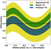 |
Fig. 12. Stellar filling factor, i.e., the ratio of the stellar radius to the Roche-lobe radius, as a function of the orbital phase (0 is mid-eclipse). Each colored stripe is obtained for a different set of extreme values observationally derived by Quaintrell et al. (2003), Rawls et al. (2011), and Falanga et al. (2015). |
4.2.2. Magnetospheric accretion and induced torques
Following its formation, a pulsar spins down first due to its autonomous magnetodipole radiation (Pacini 1968; Gunn & Ostriker 1969). After a few thousand years, it spins down at a higher pace due to the torques associated with the repelling of infalling stellar material that is ejected during the propeller phase (Francischelli et al. 2002). After this, the magnetospheric and corotation radii are expected to be similar because the torques applied by the accreted flow onto the neutron star magnetosphere tend to spin it up (spin it down) if the corotation radius is larger (smaller) than the magnetospheric radius (see Ho et al. 2020, for a study of the long-term evolution toward spin equilibrium that covers these three phases). Because this equilibrium phase is reached within only a few 10 kyr, a first attempt to estimate the neutron star magnetic field from its spin period and the mass accretion rate can be made assuming that the magnetospheric radius and the corotation radius match. The corotation radius of the neutron star in Vela X-1 can be accurately deduced from the mass of the neutron star and from its spin period,
In addition to being stable over timescales shorter than years, the corotation radius is known with a 10% precision given its low dependence on the mass and spin period of the neutron star. On the other hand, the expression that determines the magnetospheric radius depends on the geometry of the accretion flow (planar, disk, spherical), but an order-of-magnitude estimate can be obtained from (Lamb et al. 1973; Wang 1996)
where the inertia moment of the neutron star is computed assuming a uniform sphere (i.e., 2MR2/5), where an accretion rate of 2 × 10⁻¹⁰ M⊙ yr−1 corresponds to an accretion luminosity of 4 × 1036 erg s−1 for a conversion factor of 35%, and where we used the definition of a magnetic dipole μ as BR3/2.
At equilibrium, the magnetic field should be such that these two radii are equal. With numerical values coherent with those deduced for Vela X-1, we obtain an estimate of the magnetic field of B ∼ 2.2 × 10¹⁴ G. This value is at odds with what was measured relying on the CRSFs diagnostics (see Sect. 3.1.5). Fürst et al. (2014) measured a cyclotron line energy corresponding to a magnetic field B ∼ 2.6 × 10¹² G, which is two orders of magnitude smaller than the value derived assuming spin equilibrium. The serious mismatch between the magnetic field values independently deduced from the corotation radius and from CRSFs in Vela X-1 would mean that the neutron star has been spun down to a spin period much higher than the equilibrium spin period set by the torques predicted by Ghosh & Lamb (1979b) and corresponding to the estimated mass accretion rate. This is probably the strongest theoretical point that can be made against the presence of a permanent disk beyond the neutron star magnetosphere in Vela X-1. The magnetic field required to account for the observed neutron star spin variations is also higher than the field measured by the CRSFs diagnostics by two orders of magnitude (see Staubert et al. 2019, for a detailed discussion).
Alternatively, this overbraking could be indicative of a phase in the past in which stellar material was supplied to the neutron star at a much lower rate than today, and with a high amount of specific angular momentum, which is suggestive of a slow wind (Wang & Tong 2020; Ho et al. 2020). The system would have been in the propeller regime, and the neutron star would have spun down until the mass accretion rate suddenly increased by so much that the magnetospheric radius became smaller than the corotation radius, as is currently observed if the magnetic field measured through CRSFs is accurate. We must acknowledge, however, that this scenario requires a fine-tuning of the increase in mass accretion rate, of the initial magnetic field, and of the magnetic field decay, which is unlikely. In what follows, we rely on the magnetic field value obtained by direct measures through CRSFs, that is, B ∼ 2.6 × 10¹² G.
The first conclusion to draw from this value of the magnetic field is that in Vela X-1, the neutron star is never expected to be in the propeller regime. In Eq. (11), the X-ray luminosity that is required for the magnetospheric radius to be as large as the corotation radius is about 1032 erg s−1. This threshold is too low to be compatible even with the lowest observed X-ray flux values (Liao et al. 2020). For the propeller effect to be triggered, a drop in mass accretion rate by 3–4 orders of magnitude compared to its median value would be needed (Bozzo et al. 2008; Doroshenko et al. 2011). For a realistic wind microstructure, the inter-clump environment is therefore insufficiently empty to cause such a drop (Sundqvist & Puls 2018), notwithstanding the lowered variability due to the mixing of the wind material at the hydrodynamics shock (El Mellah et al. 2018).
In spite of the absence of the propeller accretion regime in Vela X-1, we do observe month- to year-long episodes of spin-up and spin-down. Each phase occurs at a steady spin period rate: ∼7 × 10⁻⁴ s day−1 to ∼ × 10−3 s day−1 for spin-up and ∼10−4 s day−1 for spin-down (Malacaria et al. 2020). They are separated by sudden torque inversions, and the net spinning up over the past decades is compatible with zero. In neutron-star-hosting HMXBs in general and in Vela X-1 in particular, the spinning up or down of neutron stars has long been attributed to the coupling between the accreted material and the magnetic field of the neutron star. As described in Sect. 2.3, the modalities of the coupling differ between the quasi-spherical and disk geometries, which both lead to different accretion-induced torques onto the neutron star magnetosphere. For disk accretion and given the parameters of Vela X-1, the torque applied to the neutron star computed by Ghosh & Lamb (1979b) spins it up and produces a spin period derivative of approximately (Ho et al. 2014; Malacaria et al. 2020)
For a quasi-spherical geometry, the evolution of the neutron star spin period depends on the accretion regime. The transition from the direct accretion regime to the subsonic propeller regime occurs when the mass accretion rate decreases below 4 × 1036 erg s−1, which corresponds to the median X-ray luminosity of Vela X-1 (Shakura et al. 2012). Then, both regimes should occur in this system. Shakura et al. (2012) set the theoretical framework for computing the accretion-induced torques applied by a quasi-spherical flow onto the magnetosphere. Shakura et al. (2018) interpreted the absence of net spinning-up or -down of the neutron star over the past decades as an indication that the system must be in spin equilibrium. Based on this assumption and on the observed spinning-up and -down rates in Vela X-1, they estimated the value of the dimensionless parameters of their model, which encapsulate the physical mechanisms at stake at the outer rim of the magnetosphere. With the parameters of Vela X-1, it yields the following spinning-up and -down torques for Vela X-1:
respectively, where Rsh is the distance from the bow shock to the neutron star, which typically is on the order of Racc/5 (El Mellah & Casse 2015), Ṗsph,− weakly depends on the system parameters, and only the two strongest dependences are shown for the spin-up rate. These values are to be compared to the spin period derivatives measured in Vela X-1, which are about 0.25–0.5 s yr−1 (spin up) and 0.05 s yr−1 (spin down, Malacaria et al. 2020). In contrast, the quasi-spherical subsonic settling model predicts higher spin-down than spin-up rates: While the predicted spin-up rate is on the order of the observed rate, the spin-down rate is overestimated by more than an order of magnitude. Furthermore, in the moderate coupling regime, Vela X-1 is expected to accrete. In this regime, a correlation of the value of the observed spin period derivatives and the X-ray luminosity is expected but has not been reported. These inconsistencies might be due both to the numerous unknowns of this model and to the strong dependence of the spin-up rate on the location of the bow shock with respect to the accretion radius, which like the relative wind speed is unknown to within at least a factor of 2. Finally, in the supersonic accretion regime of the quasi-spherical settling model, the neutron star is generally spun up by accretion-induced torques. Spinning down can only occur if the neutron star spin axis is upside down with respect to the orbital angular momentum axis, or if clumps carry enough angular momentum to momentarily cause an inversion of the sign of the accreted net angular momentum.
4.3. Emission from the accretion column or polar cap
Most of the hard X-rays we observe are produced very close to the neutron star within the accretion column. In this column, the hot in-falling plasma can upscatter through Compton-interaction seed photons to very high energies that roughly resemble the observed continuum spectrum (Davidson 1973; Davidson & Ostriker 1973; Meszaros & Nagel 1985a; Rebetzky et al. 1988). However, because the problem is complex, these early models had to make many simplifying assumptions, such as reducing the problem to 1D or neglecting the accretion flow dynamics. When they escape the accretion column, the photons cool the plasma and prevent a full thermalization of the flow (Arons et al. 1987). The source of the seed photons is still debated: A large part very likely is due to cyclotron radiation (Nagel 1981; Bussard et al. 1985; Arons et al. 1987), but thermal photons from the accretion mound on the neutron star surface will also play a role (Becker & Wolff 2005a).
While this basic idea of Comptonized photons agrees roughly with the observed spectra, detailed modeling of the spectrum produced in the accretion column continues to be difficult even with modern computers. These difficulties mainly arise because for a correct description of the particles and their interaction within the column, a full quantum-mechanical as well as relativistic treatment is necessary. In particular, the electron cross-sections are strongly polarization dependent and are increased at the cyclotron energy by orders of magnitude (e.g., Daugherty & Harding 1986, see also Sect. 4.4), which is computationally expensive to model. Additionally, the open question remains of where and how the in-falling plasma is decelerated (e.g., Becker & Wolff 2005a).
In the past decade, Becker & Wolff (2005a,b, 2007); Becker et al. (2012) have presented a more detailed model of the spectral formation in the accretion column, taking bulk (first-order Fermi acceleration) and thermal Comptonization into account and injecting seed photons from bremsstrahlung, cyclotron radiation, and thermal contribution. This model is able to reproduce the spectral shape of a few selected X-ray binaries, but requires a simplified description of the velocity in the accretion column and does not account for the variability of theses sources (Wolff et al. 2016). It assumes a high luminosity, in which a radiation-dominated shock is formed above the neutron star surface and decelerates the in-falling plasma to subsonic speeds.
Farinelli et al. (2012, 2016) expanded on the model by Becker & Wolff (2007), allowing for different velocity profiles and a magnetic field gradient within the accretion column. Their model allowed them to report a satisfying description of the X-ray spectra of bright sources such as Her X-1 and 4U 0115+63.
Vela X-1 only rarely exhibits luminosities above 1037 erg s−1. It is therefore unclear whether a radiation dominated shock forms. This intermediate-luminosity range is in particular hard to model because it is unclear which approximations can be made. Vela X-1 also shows a complex pulse profile, which might indicate that both fan and pencil beam components are present. The most recent update of the Becker & Wolff models was presented by West et al. (2017a,b), but the model has not yet been applied to Vela X-1.
The observed pulse profile strongly depends on the assumed emission profile of the accretion column and of the polar cap, and also on light-bending effects around the neutron star. For the emission geometry, two simple approximations are often made: a slab, or a column geometry. In the slab geometry, the accretion mainly escapes from the sides of the accretion column (and perpendicular to the magnetic field) close to the neutron star surface, creating a so-called fan-beam pattern (i.e., in a similar configuration as a polar cap). In a column geometry, the emission escapes along the column and parallel to the magnetic field, forming a pencil beam, with a certain (narrow) opening angle (Meszaros & Nagel 1985b; Meszaros & Riffert 1988).
While these two different geometries predict significantly different pulse profiles (Meszaros & Nagel 1985b; Wang & Welter 1981), they prove difficult to compare with observations. The observed profiles are highly complex and strongly energy dependent (see Sect. 3.1.7), and this makes them far more complicated than simple models predict.
Over the years, various efforts were made to offer physical descriptions of the pulse profile shapes. Early studies were concerned with the physical production region of the X-rays and their emission geometry. They found that the models were able to match the data for Vela X-1 approximately (e.g., Wang & Welter 1981; Leahy 1990; Sturner & Dermer 1994). However, the omission of gravitational light-bending led to unrealistic estimates of the emission geometry (Riffert et al. 1993; Leahy & Li 1995; Kraus et al. 1995).
More detailed work led to descriptions of profiles for single sources, using a large number of assumptions (Kraus et al. 1995; Caballero et al. 2011; Falkner 2018). Recently, models have been presented that allow the user to be very free in the choice of geometry and emission pattern, and they no longer require many of the previous assumptions (Cappallo et al. 2017; Falkner 2018). However, the sheer number of free parameters and large degeneracy between them has so far made it impossible to identify unique solutions. Some of the most relevant physical parameters are the amount of relativistic boosting of the in-falling plasma, the size and mass of the neutron star, and the configuration of the magnetic field. For Vela X-1, no recent physical description of the pulse profile has been put forward at the time of this review.
4.4. Cyclotron resonant scattering features
As explained in Sect. 2.4, the CRSF features that are visible in broadband X-ray spectra of Vela X-1 (see Sect. 3.1.5) are caused by resonant scattering of X-ray photons at the corresponding energies on electrons with quantized motion perpendicular to the magnetic field. Calculating the scattering cross-sections requires detailed fully relativistic QED-based calculations. Over the decades, such calculations have been undertaken by various authors and have included increasingly complex details (e.g., Harding & Daugherty 1991; Sina 1996; Isenberg et al. 1998a,b; Araya & Harding 1999; Schönherr et al. 2007). The most recent treatment based on elaborate Monte Carlo calculations is presented in Schwarm et al. (2017b,a).
The scattering cross-sections are very strongly peaked close to the Landau level energies, up to several orders of magnitude compared to Thomson scattering. This makes the plasma optically very thick for photons at these energies. Because the energy of the electrons is only quantized in the direction perpendicular to the magnetic field, however, the angle between the magnetic field and the photon becomes relevant. For large angles, the cross-sections become thermally broadened and shift to higher energies for the harmonic levels. An open question in CRSF research is the fact that model calculations (Araya & Harding 1999; Schwarm et al. 2017a,b) tend to predict asymmetrical lines, frequently showing emission wings at energies below and above the central energy, while observed features tend to be broad, without a marked asymmetry, and without a clear sign of the predicted emission features.
In order for discrete CRSFs to be observable, the sample magnetic field has to be confined to a very narrow range, indicating a closely confined region within the accretion column, possibly a shock region in the column or close to the poles (Becker & Wolff 2007, and references therein). The often observed relatively broad and shallow CRSFs might arise because multiple line-forming regions contribute (Nishimura 2008). Poutanen et al. (2013) proposed another explanation according to which, CRSFs are formed due to reflection of the downward-beamed radiation from the accretion column on the neutron star surface around the poles.
The strong angular dependence of the line features predicted in theoretical calculations would in principle lead to another diagnostic for possible emission geometries from the pulse phase, and thus geometrically, resolved spectroscopy. This is limited by the fact that because of gravitational light-bending, we can expect that multiple zones of the accretion column or neutron star surface contribute at least most of the time (Falkner 2018). We would therefore also need to have a good grasp on separating these mixed contributions.
4.5. Variability of the observed X-ray emission
In variability studies, the two privileged simulation outputs to be compared to observations are occurrence diagrams and power spectral distributions. While the first show the fraction of time that a variable spends at a given value (e.g., the mass or angular momentum accretion rates, or the column density), the second retains the information and reveals coherence timescales and possible periodicities.
4.5.1. Variable absorption along the line of sight
The mass-loss rate from the donor star is high, therefore absorption along the line of sight from the neutron star to the observer is high but is also variable (Sect. 3.1.3). Because we observe Vela X-1 close to edge-on, we expect a periodic modulation of the column density as the neutron star orbits the blue supergiant. The average orbital NH profile grants access to the orbital parameters and to the stellar mass-loss rate, provided estimates are available for the wind speed and the stellar radius. The origin of the stochastic variability of the measured absorbing column density at a given orbital period is threefold. It can be due either to changes in the amount of material that is integrated along the l.o.s. because of clumps in the stellar wind or because of a change in the flow structure near the neutron star magnetosphere, or modifications in the opacity of the medium can cause it through changes in the wind ionization structure.
Regardless of whether they participate in the accretion process, clumps intercepting the l.o.s. will produce a variability in column density on short timescales. Oskinova et al. (2012) designed a 2D model of massive (3 × 10²¹ g) and intermediate-size clumps (2% of the stellar radius at one stellar radius above the stellar photosphere) that propagate radially from the donor star. They computed the extinction coefficient as a function of time and showed how clumps that are compressed in the radial direction tend to produce a higher level of variability than their spherical counterparts (see also Oskinova et al. 2006). Grinberg et al. (2017) estimated the characteristic amplitude and timescale of absorption episodes with a simple model of clumps, to be compared to column densities derived from hardness monitoring with time-resolved spectroscopy at orbital phase ϕ ∼ 0.25. This motivated a comprehensive exploration of the NH variability induced by a clumpy wind: El Mellah et al. (2020b) designed a 3D model of clumps flowing radially away from the star with different velocity profiles, orbital parameters, and clump properties. Vela X-1 was one of the two HMXBs to which the model was applied. The authors computed the median NH orbital profile over many orbital periods, along with the standard deviation and coherence timescale at each orbital phase. The timescale was found to be associated with the flyby time of the smallest clumps along the l.o.s., which granted access to their spatial extent. Based on the porosity length, the authors also showed that the mass of the clumps could be constrained based on the standard deviation of the column density: Because they are rarer, higher-mass clumps produce a higher spread of the measured column density at a given orbital phase.
Manousakis et al. (2012) computed the structure of a smooth stellar wind in hydrodynamics numerical simulations in the orbital plane. Although their model was tailored to another high-mass X-ray binary and not to Vela X-1, they were able to reproduce the excess of column density at orbital phases 0.4–0.8 reported in Manousakis & Walter (2011) for IGR J17252−3616 and traced its origin back to an overdense accretion wake trailing the neutron star. In Vela X-1, Malacaria et al. (2016) measured episodic enhanced absorption events near inferior conjunction. They performed a detailed spectral analysis that showed that the data could be attributed to an inhomogeneous accretion wake, in agreement with the idea proposed by Doroshenko et al. (2013). The eccentricity of the orbit also introduces a minor asymmetry between the evolution of the column density when the neutron star moves toward and away from Earth.
Finally, intrinsic variations of the X-ray ionizing emission from the immediate vicinity of the neutron star (see Sect. 4.5.2) alter the wind ionization structure. The highly ionized fraction of the wind, near the neutron star and in low-density regions, is transparent to X-rays and does not contribute to the absorbing column density. It induces NH variations even if the amount of material integrated along the l.o.s. remains unchanged.
While off-states have usually been explained as due to a quenching of the accretion itself (see Sect. 4.5.2), one model found that the lowered luminosity during off-states might be due to scattering of hard X-rays along the line of sight: Sidoli et al. (2015) reported different off-state occurrence rates at orbital ingress and egress that they interpreted as an indication that off-states were due to X-rays that were being scattered in the photoionization wake identified by Blondin et al. (1990) in numerical simulations.
4.5.2. Variability in mass accretion rate
The dominant mechanisms responsible for the intrinsic variability in mass accretion rate in Vela X-1 have not yet been conclusively identified. Periodic changes are expected because the eccentricity of the neutron star orbit leads to non-negligible systematic differences in the mass density of the environment in which the neutron star is embedded: Notwithstanding wind acceleration and nonisotropic effects, the density at periastron would be 40% lower than the density at apastron. This number is a lower limit because the wind is still accelerating at the orbital separation and is more strongly beamed toward the neutron star at periastron, when the filling factor is the highest (see Sect. 4.2.1). Concerning the stochastic variability of the mass accretion rate onto the neutron star surface, the very location of its origin varies from one model to the next.
The X-ray ionizing feedback has long been suspected to modulate the mass supply onto the neutron star in an unstable manner: An increase in X-ray luminosity leads to a slower wind because the line acceleration is inhibited, which increases the mass accretion rate (see Sect. 4.2.1). The cycle closes when wind acceleration is so inhibited that stellar material no longer penetrates the Roche lobe of the neutron star. In an attempt to quantify this effect, Ho & Arons (1987b) designed a 1D model along the line that joins the two bodies with a prescribed smooth and isotropic wind. They equated the accretion X-ray luminosity associated with the BHL formula (4) with the X-ray luminosity corresponding to the extent of the region around the neutron star in which the ionization parameter is above ξcrit = 104 erg cm s−1. Using the orbital parameters of Vela X-1, they obtained two solutions. In the first, the wind was hardly affected by the X-ray ionizing feedback and yielded an X-ray luminosity corresponding to the one observed in Vela X-1. This solution was later found by Ho & Arons (1987a) to be prone to fluctuations with realistic timescales (see, e.g., Kreykenbohm et al. 2008). In the second solution derived by Ho & Arons (1987b), the X-ray luminosity was about four orders of magnitude higher, with a wind speed significantly lowered by line-acceleration quenching. In spite of episodic flares in which Vela X-1 reaches a few 1037 erg s−1, the system has never been observed in such a high state, however. Karino (2014) performed a similar computation, but accounted for optical depth and a gradual effect of the X-rays on line acceleration. Karino (2014) retrieved a bimodal behavior, but in contrast to Ho & Arons (1987b), Vela X-1 was lying on the branch corresponding to a high luminosity, associated with a slow wind. Manousakis & Walter (2015a) revived the role of the X-ray ioninzing feedback that they found to be a possible origin of the observed off-states. In 2D hydrodynamic simulations in the orbital plane, they found that when wind acceleration was inhibited above a critical ionization parameter of 102.5 erg cm s−1, a permanent X-ray luminosity of 4 × 1036 erg s−1 could produce an oscillation of the position of the accretion front shock. This breathing mode induces a subsequent modulation of the mass accretion rate onto the neutron star, with ∼30-min-long off-states during which the accretion is quenched, separated by a characteristic duration that agrees reasonably well with the characteristic timescale of the X-ray emission from Vela X-1 reported in Kreykenbohm et al. (2008). Recently, Bozzo et al. (2020) designed a detailed semianalytical model of a smooth spherically symmetric wind and showed that accounting for the eccentricity of the orbit in a simplified model of accretion leads to an average mass accretion rate almost three times higher near periastron than near apastron. Because the accretion wake intercepts the line of sight at orbital phases 0.4–0.8, precisely when the neutron star is near apoastron, it is difficult to separate between a decrease in intrinsic emission and an increase in absorption, even using hard X-ray observations. The authors also included the X-ray ionizing feedback and found that its effect was limited to the vicinity of the neutron star. This challenges the conclusions drawn by Manousakis & Walter (2015a) about the origin of off-states, but agrees with Sander et al. (2018).
Because its structure is inherently clumpy, the line-driven wind from the donor star provides material to the neutron star at variable rates. In a seminal study, Ducci et al. (2009) designed a statistical model of clump capture in which they accounted for this component by assuming that each clump intersecting the disk of radius Racc around the neutron star is instantaneously captured, with a correction factor if the overlap is only partial. They found occurrence diagrams consistent with what is observed in Vela X-1. However, these results were challenged by 3D hydrodynamic simulations of the accretion of a clumpy wind. El Mellah et al. (2018) showed that clumps were strongly compressed, distorted, and eventually mixed within the shocked region. The bow shock that forms around the neutron star significantly decreases the peak-to-peak variability compared to what is expected in the ballistic BHL framework, in which clumps are instantaneously accreted without accounting for their thermodynamical properties. These results indicate that the intrinsic variability of the X-ray emission cannot be considered a direct tracer of the wind microstructure and that other mechanisms are likely to dominate the intrinsic variability of the emission. We note that in simulations of accretion onto supermassive black holes mediated by a centrifugal gating mechanism, Gaspari et al. (2015) found similar properties for the variability of the mass accretion rate (e.g., a log-normal occurrence diagram, indicative of self-organized criticality).
Although realistic 3D clumps per se do not produce a variability high enough to account for the changes in intrinsic X-ray luminosity, they can play a role in modifying the conditions of accretion at the neutron star magnetosphere. Due to the proximity between the magnetospheric and circularization radii in Vela X-1 (see Fig. 2), the accretion flow between the shock and the magnetosphere in Vela X-1 might transit between a disk-like and a spherical geometry, depending on the instantaneous and local wind properties. In each geometry, there are regimes of low and high mass accretion rates, depending on the stellar material supplied at the orbital scale (see Sect. 4.2.1). Transitions between regimes and/or geometries might contribute to the overall variability. Bozzo et al. (2016) investigated this scenario in a model of accretion of a clumpy wind accounting for the magnetic and centrifugal gating mechanisms. They showed that for orbital and neutron star spin periods close to the ones in Vela X-1, switches between regimes were occurring. Even if the authors warned the readers about the limitations of their model, which is uni-dimensional and does not solve the wind dynamics, their work highlighted the importance of considering the coupling between the plasma and the magnetosphere to fully appreciate the evolution of the intrinsic X-ray variability.
4.6. Evolutionary scenario
High-mass X-ray binaries are an important evolutionary stage on the way to form compact object binaries and thus an interesting benchmark to understand the origin of gravitational wave sources. With a neutron star being the compact object, Vela X-1 is a candidate for either a black hole-neutron star merger or a double neutron star merger, assuming the system remains bound after the current supergiant component has undergone core collapse. The identification of the evolutionary scenario for an individual system such as Vela X-1 is complicated. Given the high number of parameters in binary evolution and the different possible channels, a snapshot of the present status can thus only be used to rule out certain scenarios rather than pinpointing at a particular evolutionary track.
Neglecting any scenarios that could involve higher-order systems, the standard scenario to form an HXMB considers two massive stars with an uneven, but not too extreme mass ratio (e.g., Tauris & van den Heuvel 2006). The more massive primary star evolves faster and eventually fills its Roche Lobe, which will lead to mass transfer from the primary to the secondary (e.g., Paczyński 1971; van den Heuvel 1976). Depending on the nuclear burning status of the primary, this is referred to as either case A (during central H-burning), case B (after central H burning, but before central He burning), or case C (after the start of central He burning) mass transfer. For typical separations and assuming close mass ratios, this first mass transfer period in the system is generally assumed to be stable (e.g., Podsiadlowski et al. 1992; Ritter 1999; de Mink et al. 2008). The mass transfer will stop after a large fraction of the hydrogen envelope has been removed from the primary. The secondary has now gained hydrogen-rich matter. Depending on the precise parameters, the secondary could now even evolve faster than the primary and reach core collapse first (e.g., Pols 1994). However, given that the mass transfer might have happened in an already advanced stage of the primary, the primary as the first object to undergo core collapse is the more common outcome. If the system remains bound beyond this stage (Blaauw 1961), we are left with a compact object resulting from the primary and a secondary which has gotten additional material and – depending on the mixing timescale of this “new” material into the deeper layers – has been “rejuvenated” (e.g. Braun & Langer 1995). Once the compact object is able to accrete matter from the secondary – either by wind accretion or Roche Lobe overflow (RLOF) – the system will appear as an HMXB.
In the case of Vela X-1, the compact object is a neutron star and the secondary has a current mass on the order of 20 M⊙. Consequently, we would expect a primary more massive than that with suggestions going up to 60 M⊙ (Quast et al. 2019). Given that enough mass needed to be removed to eventually yield a neutron star as the compact object, the latter number might be a bit high, but illustrates the severe uncertainty when trying to extrapolate the systems’ backstory. Even taking into account the accompanying supernova during the formation of the neutron star, the core mass of the primary had to be low enough to avoid the formation of a black hole, which means that either the primary mass had to be low enough or the mass transfer was efficient enough to alter the evolution before a more massive core could be formed (e.g., Wellstein & Langer 1999).
The near-circular orbit of Vela X-1 prompts the questions whether the first mass transfer in the system might have lead to a Common Envelope (CE) phase (Paczynski 1976). Even though many uncertainties remain on the detailed physical processes involved in CE evolution, their occurrence is typically inferred from an evolutionary necessity (e.g., Ivanova et al. 2013). CE stages are thought to occur for unstable RLOF and help to shrink and circularize the orbit, at least if the system can eventually eject the envelope and avoid merging. However, CE stages are unlikely to occur for the first mass transfer stage in an HMXB (Tauris & van den Heuvel 2006). The parameters for Vela X-1, including its “runaway” nature (Kaper et al. 1997, see also Fig. 14), indeed point more towards this standard scenario (van den Heuvel 2019).
The remaining secondary in Vela X-1 is classified as “overluminous” (e.g., Wickramasinghe 1975; Conti 1978). This term generally refers to that fact that the object is more luminous than expected for its mass, although the details differ in whether this refers to a simple comparison with single star evolution (e.g., Quast et al. 2019) or is also used for remaining discrepancies in the context of binary evolution scenarios (e.g., Vanbeveren et al. 1993). Regardless of terminology, it is important to account for the fact that the secondary has been rejuvenated and thus will usually have a different luminosity and temperature compared to a single star of the same spectral type.
The recent atmosphere analysis of HD 77581, the donor of Vela X-1, yields log L/L⊙ ≈ 5.5 (see Table 5). Relying on stellar structure calculations by Gräfener et al. (2011), a single star on the zero age main sequence with this luminosity would have a mass of approximate 47 M⊙. This is twice as large as measured (cf. Sect. 5.3). The other extreme would be a He star with a thin hydrogen layer negligible in mass. In this case, the donor star in Vela X-1 would be about 15.5 M⊙. The measured masses of about 20 M⊙ are much closer to the second case and thus illustrate that the now donor star has probably evolved considerably before gaining mass from the primary. Vanbeveren et al. (1993) deduced that the high ratio between luminosity and mass (L/M-ratio) could only be explained if the central hydrogen abundance of the secondary was already down to a mass fraction of 0.1 when it started accreting from the primary. Moreover, the star would need to have been fully convective during the accretion stage and its surface should now be enriched in nitrogen, but depleted in oxygen and carbon. The latter is indeed in line with the recent analysis by Giménez-García et al. (2016), although their determined surface hydrogen abundance of XS = 0.65 is slightly higher than the range suggested by Vanbeveren et al. (1993). However, depending on the details of the accretion into the secondary, the resulting values of XS can vary quite a bit (Hellings 1983; Braun & Langer 1995) with existing scenarios not excluding the measured abundance. In any case, the surface hydrogen abundance of the donor in Vela X-1 is below the solar value, thus giving rise to the label that the donor of Vela X-1 is “He enriched”.
The high L/M-ratio and the still rather high surface hydrogen abundance both lead to a stronger stellar wind mass loss than assumed for an isolated star of the same spectral type as stellar wind mass is significantly boosted for higher values of the so-called “Eddington parameter” Γe ∝ qion L/M (e.g., Gräfener & Hamann 2008; Vink et al. 2011; Sander et al. 2020; Sander & Vink 2020). A higher rotation rate due to angular momentum transfer in the earlier stages of the evolution would add to this. Consequently, the wind mass-loss rate of the secondary is now higher than it ever was for the secondary in the system before the onset of mass transfer.
In the standard picture, the HMXB type with a supergiant donor was seen as a relatively short-lived stage (e.g., Tauris & van den Heuvel 2006) due to the unstable nature of the mass transfer arising from the – now – high mass ratios between the donor and the compact object and due to the convective envelope of the donor. This claim has recently been challenged by Quast et al. (2019), who argue that despite the shrinking of the orbit also the donor radius is decreasing as the He surface abundance increases due to the mass transfer. This scenario would significantly prolong the HMXB stage and provide a better explanation for the relatively large number of HMXBs hosting a blue supergiant donor star in our own Milky Way. Depending on the L/M-ratio (Sander & Vink 2020), the donor could eventually appear as Wolf-Rayet star (Quast et al. 2019). Eventually, a CE stage with the compact object seems to be unavoidable (Hjellming & Webbink 1987; Tauris & van den Heuvel 2006), which would either lead to shrinking of the orbit or the eventual merger of the two stars after the formation of a so-called “Thorne–Żytkow object” (TZO, Thorne & Zytkow 1975, 1977). Recently, Oskinova et al. (2018) suggested that sgB[e] HMXBs could represent those HMXBs currently in or shortly after a CE stage. A successful ejection of the CE would remove further mass from the system, leading to a He star even if the considerations by Quast et al. (2019) were not applicable. However, a system like Vela X-1 might not survive the CE phase as van den Heuvel et al. (2017) argue that all systems with mass ratios larger than approximately 3.5 will lead to an inspiral of the compact object. In contrast, recent simulations suggest that the parameter space leading to successful CE ejection is more complex. Depending on the properties of the donor star envelope, CE evolution can be immediately followed by stable mass transfer (Klencki et al. 2021). So far, there are a lot of remaining uncertainties on the scenarios and detailed evolution calculations are missing, but given that the current mass ratio for Vela X-1 is about 10, the system would be a prime candidate for this fate and thus never form a compact object binary. Yet, the observational confirmation of this scenario is hampered by the severe uncertainties for the mass loss of lower-mass He stars (e.g., Vink 2017; Sander et al. 2020). While traditional considerations often associated He stars with a WR-type spectral appearance, this is only true if the stars have a sufficiently high L/M-ratio (Shenar et al. 2020; Sander & Vink 2020). For the case of Vela X-1, this would mean that the current donor would have to lose about 5 M⊙ – while at least keeping the current luminosity – before reaching a sufficient L/M-ratio for a WR-type mass-loss rate. Hence, the evolutionary fate of Vela X-1 is quite uncertain. However, the most expected outcome according to current considerations and known system parameters is a merger of two components in a CE stage (e.g., Belczynski et al. 2012). The inspiral of the neutron star into the core of the now secondary will eventually lead to the formation of a black hole. This could give rise to a less common type of short gamma-ray bursts (Fryer et al. 2013).
In addition to our knowledge of its evolutionary track, Vela X-1 was shown to move at high speed (∼90 km s−1) with respect to its local environment. This is likely indicative of the natal kick produced by the asymmetric supernova explosion when the neutron star formed, probably a few million years ago (see Sect. 5.1.2). A bow shock associated with Vela X-1 was found by Kaper et al. (1997) based on its Hα emission. Although its main axis is consistent with the relative motion of Vela X-1 through the interstellar medium, Gvaramadze et al. (2018) identified nonsymmetric features in the vicinity of the shock, such as an elongated Hα-emitting structure. Based on magnetohydrodynamic simulations, they showed that the opening angle of the bow shock and its Hα brightness could be reproduced by considering the interaction of a region of higher density in the interstellar medium with the stellar wind from the donor star in Vela X-1. Interestingly enough, they were able to reproduce the emission from the filamentary structure only by accounting for a helical magnetic field in the stellar wind that they tentatively attributed to the interaction between the stellar wind and the magnetosphere of the neutron star.
4.7. Taxonomy of wind models
Relevant models to describe the physics at stake in Vela X-1 have been published over the past decades. Most of them resorted to the numerical tool to solve the flow dynamics (e.g.,), but a handful are essentially based on (semi-)analytical approaches to study the X-ray ionizing feedback (Hatchett & McCray 1977), the flow structure (Foglizzo & Ruffert 1997), the clump capture rate (Ducci et al. 2009), the accretion mechanism (Bozzo et al. 2016), the formation of wind-captured disks (Karino et al. 2019), or the secular spin evolution of the neutron star (Karino 2020), for instance. Democratization of access to computing facilities and exploratory studies led to an overall increase in the complexity of the models that were developed to provide more detailed explanations of the physical mechanisms in Vela X-1. As an unfortunate side effect, the numerous physical and, when applicable, numerical assumptions required to capture the physics and solve the underlying equations preclude any one-to-one comparison of results, even in the rare cases when studies focus on similar aspects of the system: The price to pay for more realistic models has been an accelerated division of the system description into a constellation of models that each address more specific aspects in more detail. When observational data are not enough to decide, the robustness of the provided scenarios does not lie in the strict reproducibility of the results, but instead in the repeated occurrence of qualitatively similar features from one simulation to the next and in the compatibility of an explanation with the models proposed by other teams.
As an illustration of this difficulty of comparing different frameworks although they all solve the equations of radiative-hydrodynamics in 1D, Watanabe et al. (2006), Krtička et al. (2012, 2018), Krtička & Kubát (2017), and Sander et al. (2018) did not obtain the same wind ionization and velocity profile (see Sect. 4.1.2). The models developed by the last two teams account for more physics than in the more simplified calculation by Watanabe et al. (2006), but they both chose to rely on different assumptions concerning the frame in which the radiative transfer is performed, the ions involved in the computation, the X-ray emission, and the stellar properties or the wind clumping, among others.
Similarly, the 2D and 3D simulations ran by Čechura & Hadrava (2015), which are primarily tailored to the properties of Cygnus X-1, another wind-fed high-mass X-ray binary, Blondin et al. (1990), Manousakis et al. (2012), Manousakis & Walter (2015a,b), and El Mellah et al. (2019a) did not handle the effect of the X-rays on wind acceleration in the same way. Because of their multidimensional aspect, none of these simulations can afford to treat radiative transfer in a way as realistic as the studies above. For instance, they cannot capture any spectral property, but instead have to focus on the overall photoionizing flux, which is taken to be the X-ray flux from the neutron star. In order to represent the wind acceleration quenching, they relied on the critical ionization parameter (see Eq. (2)) beyond which the ions contributing most to the resonant line absorption are assumed to be so depleted that acceleration drops to zero. In this all-or-nothing approach, it can only be guessed which critical ionization parameter is realistic because the dominant ions are unknown and sharply depend on the stellar properties and chemical composition. Even in this case, the sudden quenching assumed by Manousakis & Walter (2015b) or the even steady decrease of the acceleration assumed by Čechura & Hadrava (2015) has been shown to be a far too simplified approximation (Sander et al. 2018). Instead, El Mellah et al. (2019a) relied on the 1D line acceleration profile computed by Sander et al. (2018) for the donor star in Vela X-1, but assumed that the nonisotropic 3D features induced by the orbital motion in their simulations had no significant effect on this profile, but were purely a function of the distance to the donor star. This hypothesis remains to be confirmed. Below the critical ionization parameter (100.5 erg cm s−1 in Čechura & Hadrava 2015, 102.5 erg cm s−1 in Manousakis & Walter 2015b), line acceleration is computed differently in these studies, leading to different amounts of specific kinetic energy that was deposited in the wind by the stellar photon field when the flow reached the neutron star.
The wind microstructure has also been treated in different ways: While some works assumed a smooth wind (Watanabe et al. 2006; El Mellah & Casse 2017; Blondin et al. 1991), others included wind clumpiness in their models or simulations. The clumps are either indirectly represented by their effect on the radiation field (Sander et al. 2018), are parameterized as spheres of a given mass and radius (Oskinova et al. 2012; El Mellah et al. 2020b), or are computed from 2D radiative-hydrodynamics simulations on pseudo-planar grids before being extended to 3D (El Mellah et al. 2018). Because of their small sizes, however, including more realistic clumps comes at the expense of a smaller simulation space in radiative-hydrodynamics simulations, or of simplified equations of motion of the flow.
A detailed taxonomy of the models of Vela X-1 in particular and of wind-fed neutron stars in supergiant X-ray binaries in general is beyond the scope of this paper. It would help to determine which model could prove fruitful in order to interpret a given set of observations, however.
5. Properties of the Vela X-1 system
In this section we compile the existing knowledge on the essential parameters of the Vela X-1 system and how they have been obtained. We also indicate where results were strongly based on parameters from previous work. The section is broken down into subsections for different essential parameters, but we note that depending on the data and analysis methods that were used, various parameters have frequently been derived jointly or cannot be determined in an independent fashion from other parameters. A trivial example are the masses of the binary partners and inclination (Fig. 17).
5.1. Distance from Earth and relation to the Vela OB1 association
In order to derive the real luminosities of the supergiant and the X-ray source, it has been the goal for many different authors to determine the distance to Vela X-1. Figure 13 illustrates the evolution of different distance estimates over time.
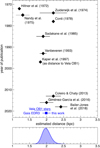 |
Fig. 13. Upper panel: evolution of distance estimates to the Vela X-1 system over time derived with different approaches, as explained in the text. At the bottom we also show the distance ranges derived for stars in the Vela OB1 association and our new distance determination based on the new Gaia-EDR3 data. Lower panel: posterior distribution of our updated Gaia distance estimate. |
5.1.1. Evolution of the distance estimates
The earliest distance estimate to the Vela X-1 system, or more precisely, to HD 77581, was reported by Hiltner et al. (1972), who derived a distance of 1.2 kpc (distance modulus 10.5) based on an assumed absolute magnitude of MV = −6.0 and a ratio of 3.0 for the total-to-selective absorption. This distance estimate was still used as a baseline in the 1980s, for instance, by Nagase et al. (1984a). Based on UV observations with the European satellite Thor-Delta 1A (TD1), Nandy et al. (1975) arrived at a similar result of 1.3 ± 0.2 kpc.
In contrast, Wickramasinghe et al. (1974) derived a distance > 2 kpc by comparing the reddening of HD 77581 with that of stars in its vicinity. Zuiderwijk et al. (1974) used the equivalent width of interstellar Ca II K, independent from the reddening diagnostics, to derive a distance of 2.2 ± 0.4 kpc.
Based on the spectral type (Hiltner et al. 1972) and duration of the eclipse (Forman et al. 1973), Conti (1978) derived a stellar radius of 35 R⊙ and an absolute magnitude MV = −7.0, which then led to an estimated distance of 2.2 kpc (no uncertainty given) based on the photometry by Jones & Liller (1973).
Sadakane et al. (1985) used ultraviolet spectra obtained with IUE to determine an effective temperature of 25 000 ± 1000 K. They combined this temperature with a radius of 31 R⊙ (Rappaport & Joss 1983) to arrive at an absolute visual magnitude MV = −6.67 and a derived distance of 1.9 ± 0.2 kpc.
From a spectroscopic analysis using NLTE models (see Sect. 3.2.3), Vanbeveren et al. (1993) derived a distance of 1.8–2 kpc.
Kaper et al. (1997) noted the possible connection to the Vela OB1 association (see below) and introduced the distance of 1.82 kpc to the Vela OB1 (Humphreys 1978) as a distance value. This was then used by several subsequent X-ray studies without considering the implied uncertainties.
Coleiro & Chaty (2013) used a spectral energy distribution (SED) fitting procedure in order to derive the distance and absorption of a sample of HMXBs. For Vela X-1, they derived a value of 2.2 ± 0.2 kpc.
This approach was further refined by Giménez-García et al. (2016). They combined data from IR (2MASS) to UV (IUE) for the SED with a detailed analysis of spectral lines using NLTE models created with the PoWR code (see Sect. 3.2.3) in order to derive the extinction, luminosity, and distance to the source, arriving at a distance of 2.0 ± 0.2 kpc.
In the huge catalog of stellar distances based on Gaia Data Release 2 (Gaia DR2, Gaia Collaboration 2018) parallaxes, published by Bailer-Jones et al. (2018), the distance to Vela X-1 is derived as 2.42 − 0.16 + 0.19 kpc from a Bayesian analysis, with a basic parallax of 0.38 ± 0.03 μas. Figure 13 shows that this distance is farther away than most previous estimates and is formally consistent with only very few estimates.
The recently published third Gaia data release (EDR3, Gaia Collaboration 2021) gives us the opportunity to obtain an improved distance to Vela X-1. Gaia EDR3 lists a parallax ϖ = 496.2 ± 15.2 μas. To derive a distance, we first applied a parallax zero-point of −13.5 μas using the Lindegren et al. (2021a) recipe for the relevant magnitude, color, and ecliptic latitude. For this specific star, this zero-point does not differ much from the median quasar value of −17 μas, but we note that a star as bright as Vela X-1 (GEDR3 = 6.7351) is at the limit of the analysis in Sect. 4.4 of Lindegren et al. (2021a). Next, we considered transforming from the internal parallax uncertainty of 15.2 μas to an external uncertainty. Following Lindegren et al. (2018), astrometric uncertainties should be transformed from their internal (σi) to their external (σe) uncertainties using
where k is a value to be determined (and likely a function of at least magnitude), and σs is the square root of the limit when the angular covariance reaches zero. As of the time of this writing, the value of k has only been estimated for stars significantly fainter than Vela X-1 (Fabricius et al. 2021; Maíz Apellániz et al. 2021). We used a value of k = 1, which may be a slight underestimation, but we compensate for this by using a very conservative value of 26 μas for σs, which is derived from (faint) quasars by Lindegren et al. (2021b) and is likely to be an overestimation because the checkered pattern seen in the EDR3 data for the LMC has a smaller amplitude (Lindegren et al. 2021b). In this way, we arrive at a corrected parallax of ϖ = 509.7 ± 30.1 μas, which may be revised in the near future when the systematic uncertainties in Gaia EDR3 are better characterized. Using this parallax as an input and the prior for runaway OB stars from Maíz Apellániz (2001), Maíz Apellániz et al. (2005) with the updated parameters from Maíz Apellániz et al. (2008), we arrive at a distance of  kpc for Vela X-1. We note from the analysis of Pantaleoni González et al. (2021) with Gaia DR2 data (which should also apply to the EDR3 case) that when a reasonable prior is used for the stellar spatial distribution in the Galaxy, distances for stars with precise Gaia parallaxes are robust, that is, they are nearly independent of the specific prior, especially for objects within a few kiloparsec.
5.1.2. Possible origin in the Vela OB1 association
In a wider study of six stars and four OB associations, van Rensbergen et al. (1996) found that Vela X-1 presumably originated in the Vela OB1 association7 (Humphreys 1978; Melnik & Dambis 2020) of massive stars. They found that HD 77581 was a runaway OB star, probably expelled from the Vela OB1 association by the natal kick that occurred during the supernova explosion associated with the formation of the neutron star.
The connection with Vela OB1 was again reported by Kaper et al. (1997), who discovered a symmetric wind bow shock about 0.9 arcmin north of HD 77581 in a narrow-band Hα image. This bow shock is created by the balance between the ram pressure of the stellar wind and the ambient interstellar medium, not to be confused with the much smaller bow shock that formed between the blue supergiant and the neutron star by the motion of the latter in the stellar wind of the former (Sect. 2.3). Based on the symmetry axis of the bow shock, they proposed a different direction of proper motion than was assumed by van Rensbergen et al. (1996). They also noted that the distance of 1.82 kpc to Vela OB1 given by Humphreys (1978) agreed with the distance to Vela X-1 reported by Sadakane et al. (1985) and the X-ray luminosity, thus popularizing the use of this distance.
In a follow-up study, Huthoff & Kaper (2002) searched for bow shocks around other HMXBs or single OB runaway stars, but found no other example in the first group and only a minority in the second. They concluded that the formation of a bow show strongly depends on the temperature and density of the ambient medium and that apparently the majority of OB runaway stars is moving through hot bubbles in the Galactic plane.
In their search for Galactic runaway stars based on the Gaia Data Release 1, Maíz Apellániz et al. (2018) found the bow shock around HD 77581 (GP Vel in that publication) also in images obtained by WISE8 and demonstrated that the proper motion taken from the Tycho-Gaia Astrometric Solution (TGAS, Michalik et al. 2015) aligned very well with the symmetry axis of the shock, provided it was corrected for the mean proper motion of OB stars in that Galactic direction (see inset in Fig. 14).
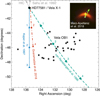 |
Fig. 14. Comparison of the proposed tracks for the Vela X-1 system relative to the Vela OB1 association following Fig. 7 of van Rensbergen et al. (1996), Fig. 3 of Kaper et al. (1997), and Fig. 7 of Gvaramadze et al. (2018). The stars shown as belonging to the association (see Sect. 5.1.2) are listed in Table A.3. The numbers along the tracks indicate where the system would have been one, two, or three million years ago, based on the assumptions in these publications. The direction of proper motion, as listed in the HIPPARCOS Input Catalog (HIC) (Turon et al. 1992) and as obtained by Sahu (1992), is shown by gray vectors. The inset is adapted from Fig. 6 of Maíz Apellániz et al. (2018) and shows a 14′ × 14′ WISE RGB mosaic. Green and yellow arrows indicate the raw and corrected proper motions, respectively (see the reference for details). The vectors shown in the inset are not to scale with those of the main drawing. |
Motivated by the results of Kaper et al. (1997), Gvaramadze et al. (2018) searched for an Hα counterpart in the Southern H-alpha Sky Survey Atlas (SHASSA, Gaustad et al. 2001). They found extended filamentary structures downstream of the bow shock within a wider area and presented the results of optical spectroscopy of the bow shock, comparing the observational data with 3D magnetohydrodynamic simulations. Recalculating the space velocity of the system (Table 2), Gvaramadze et al. (2018) confirmed the possible association with the Vela OB1 association, but warned that this connection might be spurious if the original binary system was ejected from its parent star cluster before the supernova explosion. Even the lower estimate for the actual space velocity of Vela X-1 places the system in the top few percentiles of the velocity distribution of runaway stars derived from recent numerical calculations of massive binary evolution (Renzo et al. 2019).
Space velocity estimates of the Vela X-1 system.
As found in the previous section, the distance to Vela X-1 based on Gaia data is not fully consistent with the commonly assumed mean distance to the Vela OB1 association. Therefore we also used Gaia EDR3 astrometric data to revisit Vela OB1 and obtain our own estimate of its distance.
Recently, Melnik & Dambis (2020) cross-matched the catalog of Blaha & Humphreys (1989) with Gaia DR2 using a matching radius of 3 arcsec and a magnitude tolerance of 3 mag. They identified 46 Vela OB1 sources with Gaia DR2 counterparts. We cross-matched these 46 sources with Gaia EDR3 and obtained a counterpart for all of them. However, we rejected 7 sources with poor astrometric solution (renormalized unit weight error, RUWE9, > 1.4).
We assumed that all Vela OB1 members have similar distances (parallaxes) and kinematic (proper motions). We therefore applied an iterative 3σ clipping in parallax, proper motion in RA, and proper motion in DEC. This reduced the sample to 30 Gaia EDR3 sources with compatible parallaxes and proper motions that are considered to belong to Vela OB1. They are shown in Fig. 14 and listed in Table A.3. This table contains the Gaia EDR3 ID, the coordinates of the source, and the parallax and proper motion used in this work.
Using this reduced sample, we estimated a mean parallax for Vela OB1 of 0.53 ± 0.07 mas. This corresponds to a mean distance of 1.88 ± 0.24 kpc and is based on the inverse of the parallax and error propagation alone.
The distance to Vela OB1 is therefore compatible with a possible origin of Vela X-1 in this stellar association. However, the estimated distances to Vela OB1 have large uncertainties that for the moment prevent us from reaching a firm conclusion about the origin of Vela X-1. It is expected that future Gaia data releases will allow us a better determination of the distance to Vela OB1 and Vela X-1.
5.2. Orbital parameters and ephemerides
Since the first clearly determined orbital period (Forman et al. 1973), the orbital parameters have been further refined in the following years and decades by various different groups based on eclipse timing, the analysis of Doppler shifts in the X-ray pulsations, or RVs from optical spectroscopy, for example. The values have essentially converged for the main parameters. Table 3 presents an overview of this evolution and gives the references. In the more recent literature, the orbital parameters are frequently taken from Bildsten et al. (1997) or from the updated values from Kreykenbohm et al. (2008), who largely built on the previous work. Falanga et al. (2015) have undertaken a systematic study of eclipsing HMXBs and derived new orbital parameters for Vela X-1, which slightly contradict Bildsten et al. (1997) or Kreykenbohm et al. (2008); see Table 3 and Fig. 15.
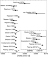 |
Fig. 15. Evolution of orbital period determinations since Hutchings (1974), converging on very similar values by different groups. |
Orbital parameters of the Vela X-1/HD 77581 system as derived by a selection of authors over the years.
Although the remaining differences are small, the orbital phases calculated using ephemerides published in the past three decades (Deeter et al. 1987a; Bildsten et al. 1997; Kreykenbohm et al. 2008; Falanga et al. 2015) agree very well, at a level of a few times 10−3 in orbital phase all the way back to the detection of Vela X-1. The systematic phase shift induced by choosing either Tecl or Tπ/2 is significantly larger, about 0.025 ± 0.01 (Kreykenbohm et al. 2008; Falanga et al. 2015). Figure 16 illustrates these facts for a recent date. Care should be taken in any discussion of orbital variations that it is clearly indicated which ephemeris and zero time is used.
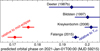 |
Fig. 16. Predicted orbital phase for a given date, demonstrating the small differences between different ephemerides. In contrast, the difference in phase between mid-eclipse time and Tπ/2 as zero-point, as shown for Kreykenbohm et al. (2008) and Falanga et al. (2015), is significant. |
The orbit of Vela X-1 is very stable and shows no indication of orbital decay. As the most recent study, Falanga et al. (2015), combining results from back to Forman et al. (1973) with data up to 2011 derived a period decay consistent with zero (Ṗorb/Porb = 0.1(3) × 10−6 yr−1). They reported indications for a slight apsidal advance ( ), in contrast with previous studies (Deeter et al. 1987b, and references therein).
5.3. Masses, radii, and inclination
Most commonly, the masses of the two components of the binary have been determined from fits to RV curves (see Sect. 3.2.2). In some cases, the mass and radius of HD 77581 have been estimated by other means. Lamers et al. (1976), for example, used half the orbital separation as the stellar radius estimate because this agreed with the mean value for these supergiants, and matched the temperature and evolutionary tracks to determine the mass of the donor star.
Early RV observations (Hiltner et al. 1972) were interpreted as indications of a possible black hole in the binary system (Wickramasinghe et al. 1974), but with more measurements, this interpretation was soon changed to a high-mass neutron star system instead, with possible masses between 1.5 and 2.9 M⊙ (Hutchings 1974). In the following years, various other authors have undertaken to determine the masses of the two partners, sometimes using the same basic data sets, but arriving at different results.
As examples of how the results of the analysis may depend on assumptions, van Kerkwijk et al. (1995) derived three different sets of solutions for different ranges of the RV amplitude Kopt derived under different assumptions: The first set is for a conservative range, set 2 is for the best fit using all their data, and set 3 for Kopt derived excluding orbital phase 0.65–0.85, in which they found the strongest indications for systematic effects. As inclination constraints for these three cases, they used i > 74, i > 73 and i > 75°, respectively. Later, Stickland et al. (1997) used the same data set as van Kerkwijk et al. (1995), but a different fitting procedure. They derived systematically lower estimates for the neutron star mass and reported three different possible solutions for (a) an unconstrained orbital fit, (b) using the orbital solution from Deeter et al. (1987b), and (c) with the spectra of the comparison star taken with a small aperture.
An interesting complementary approach was used by Bulik et al. (1995), who fit pulse-phase resolved X-ray spectra with a model of X-ray emission from polar caps in an inhomogeneous highly magnetized neutron star atmosphere. They included general relativistic effects to derive constraints on the neutron star mass and radius. Their results depend on assumptions about the emission region, however, and they reported systematic differences for fits made to different energy ranges.
Table 4 compiles different mass estimates, and Fig. 17 visualizes a selection of results for the neutron star mass in comparison with the mass distribution of other neutron stars with existing estimates.
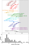 |
Fig. 17. Upper panel: selected estimates of the mass of the neutron star in Vela X-1 taken from the literature. The estimates are for specific assumed inclinations (see the original papers for how these where chosen) or plotted for a range of values with i = 90° as the lowest mass point and then 5° steps to i = 70°, to show the sin(i) dependence. See text for the multiple solutions provided by van Kerkwijk et al. (1995). The shaded areas on the right indicate possible maximum masses for neutron stars based on multi-messenger observations of GW170817 (see Margalit & Metzger 2017, and references therein). To set them into perspective, the lower panel shows the distribution of derived masses of other neutron stars in the literature taken from Alsing et al. (2018) for comparison. |
Estimated masses of the two binary components of the Vela X-1/HD 77581 system as given by various authors, together with the assumed inclination i.
In summary, while there are clear indications for a relatively high-mass neutron star in Vela X-1, with a mass of about 1.8 M⊙ or even higher, the systematic uncertainties in the derivation of the mass still allow a rather wide range of masses. The only moderately constrained inclination is a significant factor that by itself is responsible for a difference of ∼15% between the lowest and highest mass of a given study, but there is larger scatter from the different approaches. The radius of the neutron star has not been derived from observations. It will depend on the actual mass and the equation of state of the neutron star. Discussing the many solutions for the equation of state and the corresponding mass-radius relations is beyond the scope of this article (see, e.g., Lattimer & Prakash 2007, for a review), but based on the tracks shown in Maselli et al. (2020) for models compatible with current constraints, we arrive at possible radii between 11 and 12.5 km for a plausible range in neutron star masses in the Vela X-1 system. Similarly, the mass of HD 77581 is effectively constrained to a range 20–30 M⊙, while its radius is mostly found to be ∼30 R⊙.
Finally, indirect theoretical arguments and numerical approaches can also be used in favor of certain values for the mass of the neutron star. For instance, Manousakis et al. (2012) proposed a mass estimate based on the geometry of the accretion flow as deduced from the absorption column density profile: All things being equal, the higher the mass of the neutron star, the more distorted the wind they obtained in their hydrodynamical simulations, leading to different column density profiles. Although they considered another HMXB, IGR J17252−3616, as an example case, their method would be applicable to Vela X-1 as well. We also note that for a mass ratio lower than ∼12, the absence of RLOF (see Sect. 2.2) sets a more stringent lower limit on the orbital inclination than the eclipse duration.
5.4. Revising the spectral classification of HD 77581
SIMBAD lists different spectral classifications of HD 77581. They range in spectral subtype from B0 to B0.5 and in luminosity class from Ib to Ia. This means that the different authors agree that it is an early-type B supergiant, but disagree on the precise spectral classification. This disagreement is quite common for OB stars because many objects were classified in the 1950s–1970s using photographic plates, and they have not been revisited with modern digital data since then. For this reason, the Galactic O-Star Spectroscopic Survey (GOSSS, Maíz Apellániz et al. 2011) was started a decade ago. It was originally restricted to the modern spectral classification of O stars and was later extended to B stars. A GOSSS spectrogram of HD 77581 was presented in Maíz Apellániz et al. (2018) and given the classification of B0.5 Ia. Since that paper, the GOSSS team (of which the PI is a coauthor here) has revisited the spectral classification criteria for B supergiants and is currently working on a new publication on this issue. The two main criteria for the horizontal classification of early-B stars are the ratio of Si III to Si IV lines and the progressive disappearance of He II lines in the spectrum with evolution from B0 to B1. Originally, He II lines were only seen in O stars, but with improvements in S/N and the advent of digital data, the current criteria establish that for supergiants, He IIλ4542 disappears at B0.5 (and is just visible at B0.2) and that He IIλ4686 disappears at B1 (and is just visible at B0.7). HD 77581 shows a weak He IIλ4542 absorption, and the ratio of the Si III to Si IV lines is intermediate between those at B0 and B0.5. On the other hand, the ratio of the Si III to He I lines and the Hβ to Hδ profiles indicates a high luminosity class of Ia (but not Ia+ because Hβ does not show a P-Cygni profile). Therefore, we revise the GOSSS spectral classification from B0.5 Ia to B0.2 Ia.
5.5. New determination of stellar parameters
Based on newer data and our distance estimate (see Sect. 5.1), we used the latest version of CHORIZOS (Maíz Apellániz 2004) to again derive some of the parameters of HD 77581. CHORIZOS is a Bayesian photometric code that computes the likelihood that a set of photometric data is compatible with a family of SEDs.
Photometric data. We collected the magnitudes from Gaia DR2 G + GBP + GRP (Evans et al. 2018 with the corrections and calibration from Maíz Apellániz & Weiler 2018), Johnson U + B + V (Mermilliod et al. 1997 with the calibration from Maíz Apellániz 2006, 2007), 2MASS J + H + Ks (Skrutskie et al. 2006 with the calibration from Maíz Apellániz & Pantaleoni González 2018), and WISE W1 + W2 + W3 + W4 (Cutri et al. 2013). As the object has a significant IR excess, we eliminated the four photometric points with the longest effective wavelengths from the runs (the four WISE bands), but included them in the analysis to evaluate the excesses.
Models. We used the Teff-luminosity class grid with solar metallicity from Maíz Apellániz (2013b). The temperature of interest lies in the region for which the grid uses the TLUSTY models (Lanz & Hubeny 2007) in the optical and the Munari models (Munari et al. 2005) in the NIR. The reason for using these combined models is that the TLUSTY SEDs for B stars yield incorrect photometric values by up to several hundredths of a magnitude in the NIR. The Munari models do not have this problem.
Parameters. For our run we fixed the value of the logarithmic distance log d to 3.299, and we left four free parameters: Teff, luminosity class, E(4405−5495) (amount of extinction), and R5495 (type of extinction). We used the family of extinction laws of Maíz Apellániz et al. (2014), see Maíz Apellániz (2004, 2013a) and Maíz Apellániz & Barbá (2018) for an explanation of why monochromatic quantities need to be used instead of band-integrated quantities to characterize extinction. Because we fit nine photometric points, we had five degrees of freedom.
Results. The results of the CHORIZOS run are given in Table 6, and the mode SED is shown in Fig. 18. The reduced χ2 of the mode SED is 0.75, indicating an excellent fit of the model to the data. This is shown in Fig. 18, where all green stars up to Ks are within the blue error bars or very close to them. The first five lines of Table 6 give the results for the model parameters (mean, uncertainty, and mode), and the last nine lines list the results for the derived parameters (mean and uncertainty). We discuss the model parameters first.
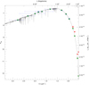 |
Fig. 18. CHORIZOS mode SED. Blue error bars are used for the input photometry that was used for the fit (Gaia DR2 G + GBP + GRP, Johnson U + B + V, and 2MASS J + H + Ks) and red error bars for the discarded input photometry (WISE W1 + W2 + W3 + W4). In each case, the vertical error bar is the photometric uncertainty, and the horizontal error bar is a representation of the wavelength coverage of each filter. Green stars are used for the model photometry. |
Teff is poorly constrained because the main discerning criterion is the Balmer jump, which is determined almost exclusively by the Johnson U − B (Maíz Apellániz et al. 2014). The value is above those obtained from spectroscopy, but within 2σ. The luminosity class is the photometric equivalent to the spectral luminosity class; it varies from 0.0 (hypergiants) to 5.5 (ZAMS). The value found by CHORIZOS (which is dependent on the fixed distance) indicates it is a bright supergiant, which is consistent with the Ia spectral luminosity classification. The extinction parameters indicate that the value of R5495 is above the canonical value of 3.1, which is relatively frequently the case for sightlines with E(4405−5495) (Maíz Apellániz & Barbá 2018), and that E(4405−5495) [or E(B − V)] is slightly lower than previous values. We note, however, that the higher value of R5495 leads to only a small change in A5495 (or in AVJ) compared to a measurement of E(4405−5495) of 0.75 assuming a value of R5495 of 3.1, for example.
The derived parameters in Table 6 were obtained with the help of the Geneva (Lejeune & Schaerer 2001) evolutionary tracks used by the Maíz Apellániz (2013b) grid and assuming the value of log d given there. The luminosity we found is close to one million in solar units with a relatively large uncertainty caused by the relatively large uncertainty in Teff (and, hence, on the bolometric correction). The values for log g, ZAMS mass, and age depend in a complex way on distance, and if different distance were to be used, they would change in a nontrivial way. In any case, taken at face value and assuming the validity of the used evolutionary tracks, the CHORIZOS results indicate that HD 77581 is a very massive star that was born less than three million years ago and that initially would have been a very early type O star or even a WNh star. Based on the existence of the neutron star companion and on the mass transfer that must have taken place in the past, the previous initial state and evolution of the star are likely to have been different. Moreover, the uncertainty in the absolute magnitude of the star in the Johnson V band is very low. This is so because (a) the extinction parameters are very well determined, (b) for this quantity we are not affected by the bolometric correction (as we are for the luminosity), and (c) we considered the distance as a fixed quantity. For a different distance, we would need to correct for the different value of 5log d.
Finally, we analyzed the behavior of the SED in the WISE bands in the MIR. There are clear excesses there that we quantify as 0.135 ± 0.066 mag (W1), 0.346 ± 0.035 mag (W2), 0.346 ± 0.027 mag (W3), and 2.007 ± 0.035 mag (W4). We note that the Munari models do not include stellar winds.
5.6. Stellar wind parameters
Over the years, many different approaches have been made to determine essential parameters of HD 77581 related to its strong stellar wind. They are collected in Tables 4, 5, and 7. As summarized in Sect. 3.2.3, one common approach based on the study of massive stars in general is through (quantitative) spectroscopy. This has ranged from the study of specific lines that were sometimes compared with samples of example stars (e.g., Wickramasinghe et al. 1974; Ammann & Mauder 1978; Sadakane et al. 1985; Prinja et al. 1990; Zuiderwijk 1995; Howarth et al. 1997), to a detailed SED analysis against grids of stellar model spectra created with increasingly refined wind model codes (Vanbeveren et al. 1993; Fraser et al. 2010; Giménez-García et al. 2016; Sander et al. 2018); see also Sect. 4.1.
Parameters of HD 77581 derived by different authors.
Detailed results of the CHORIZOS analysis.
Other authors explicitly included the X-ray source in the derivation, for example, by comparing the observed X-ray luminosity with that expected from a model of stellar wind accretion (see Sect. 2.2Lamers et al. 1976; Conti 1978) or full hydrodynamic simulations (Manousakis & Walter 2015a,b). Others modeled the Hatchett–McCray effect on line features that vary with orbital phase (Dupree et al. 1980; van Loon et al. 2001). Yet another approach is based on the modeling of high-resolution X-ray spectra (Sect. 7.1), assuming an ionized stellar wind of a certain structure, with some parameters taken as given from previous work and others then derived from the spectral modeling (Sako et al. 1999; Watanabe et al. 2006).
We also note that most of the efforts start from a smooth, nonclumped wind, even though other physical effects that are taken into account then may break the original full symmetry.
When we compare all these results, it is clear that the basic parameters of the mass donor and its stellar wind are still only known within a significant range of uncertainty. Care must be taken when astrophysical conclusions are derived from a comparison of model results with any specific value.
For the rotational velocity, the derived values vary by a factor > 2, although in all cases, HD 77581 rotates significantly more slowly than the orbital movement: by a factor of roughly one-third to two-thirds, based on the values in Table 5. Giménez-García et al. (2016), who adopted the low value of 56 km s−1 from Fraser et al. (2010). We note that the high estimates of rotational velocity are not consistent with optical lines that are observed to be unblended. Additional broadening of lines by macroturbulence (e.g., Ryans et al. 2002) may play a role in these discrepancies.
The mass-loss rate is known to within a factor of a few when more recent estimates are compared. The spread in values is within an order of magnitude when a wider range of estimates and their uncertainties from the literature are considered.
The terminal velocity v∞ shows an apparent trend with rather high values preferred in earlier studies and lower values in more current ones, even when we consider that Giménez-García et al. (2016) and Sander et al. (2018) were based on the same underlying model code. The β parameter has usually not been derived, but was set to a specific value based on assumptions about the physics of line-driven winds.
Figure 19 compares different descriptions of the stellar wind velocity around HD 77581. The profiles based on Dupree et al. (1980), McCray et al. (1984), and Watanabe et al. (2006) are β-laws (Eq. (1)). Krtička et al. (2012) used a more complex polynomial expansion in their study. In the case of Giménez-García et al. (2016), a β-law is connected to an atmosphere solution, while in the three solutions given by Sander et al. (2018), the velocity profile is determined as a solution of a hydrodynamically consistent atmosphere model describing the wind stratification.
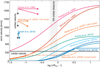 |
Fig. 19. Comparison of different derived wind velocity profiles from the literature (Table 7). See text for more details of the models. These are mostly the solutions for the wind without accounting for the ionization of the neutron star, except in the case of two of the models by Sander et al. (2018) and, at the bottom, the velocity profile calculated by Watanabe et al. (2006) along the line connecting donor and neutron star. The range of possible distances covered by the neutron star on its eccentric orbit (Bildsten et al. 1997) and the orbital velocity range, mainly driven by the uncertainty in inclination, are indicated as well. In the upper left corner we indicate approximately how wind (shown as horizontal lines) and orbital velocity (vertical) would combine at the mean neutron star distance from HD 77581 for three of the reported velocity profiles. These differences have a strong effect on the expected accretion flow close to the neutron star (see Sect. 4.1). |
5.7. Wake structures
Charles et al. (1976) reported observations of Vela X-1 with the MSSL X-ray instrument. They found indications in their data for increased absorption in a trailing accretion wake and possibly in a leading bow shock, noting that these structures varied from cycle to cycle and probably during each cycle. Referring to these results, Conti (1978) noted that a wake like this would mean that the wind velocity at the distance of the source would be on the order of the orbital velocity, that is, at much lower values than assumed in some later publications (see Fig. 19). The existence of this wake is also the commonly accepted main contribution to the high column densities observed at late orbital phases (Sect. 3.1.3 and Fig. 5).
Indications for a photoionization wake (see Sect. 4.1.2) have been found by Kaper et al. (1994) from high-resolution optical spectroscopy of the hydrogen Balmer lines and He lines and by van Loon et al. (2001) from orbital modulation through additional absorption of UV lines (see Sect. 3.2.4). Barziv et al. (2001) also explained part of their spectroscopic data with the presence of this wake (see Sect. 3.2.2). From their simulations of stellar wind disruption, Blondin et al. (1990) noted that for a photoionization wake to contribute significantly to the integrated column density, the wind would have to be ionized most of the way to the companion star.
In summary, the trailing wakes caused by the movement of the neutron star through the dense stellar wind and the added effect of the ionizing X-ray radiation play an important role in the modulation of the observed emission at many wavelengths. When models are compared to data, it is important to keep in mind that these structures can be expected to significantly vary from one orbital cycle to the next, and that the photoionization wake is also strongly affected by the significant variations in the X-ray flux (Sect. 7.2).
5.8. Strength of the magnetic field of the neutron star
When we identify the 25 keV line that is visible in the X-ray spectrum of Vela X-1 (Sect. 3.1.5) as the fundamental cyclotron line, we can use Eq. (7) to infer a magnetic field strength in the line-forming region of 2 × (1 + z)1012 G. As has been shown by Fürst et al. (2010) and La Parola et al. (2016), the first harmonic (at about 55 keV) shows a correlation with luminosity, indicating that the line-forming region changes in altitude above the surface of the neutron star. Using this correlation and theoretical calculations by Becker et al. (2012) and Fürst et al. (2010) inferred a surface magnetic field of B⋆ = 2.6 × 10¹² G. However, this value should be taken only as an estimate because it depends on the exact physical conditions within the accretion column, in particular, on the dominating process of decelerating the in-falling material, as well as on the mass and radius of the neutron star.
In principle, we could also infer constraints on the magnetic field strength from the observed torques, as has been done for other accreting X-ray sources. This type of estimate depends on many model assumptions (see Sect. 4.2.2), however, especially for a source with a potentially variable accretion geometry, and thus does not add information for Vela X-1.
5.9. Observed torques on the neutron star
Changes in the observed spin period, or equivalently, the spin frequency (Sect. 3.1.6), can in principle be used to derive information on the torques acting on the neutron star through interactions in the magnetosphere (Sect. 4.2.2). It is important to note, however, that the reported periods or frequencies are often average values over timescales of hours, days, and sometimes many weeks, which averages out short-term fluctuations. The reported changes are thus at least on the same timescales, or between data points even farther apart. In contrast, model predictions are instantaneous. A comparison between observed and predicted changes therefore implies that the characteristic timescale of a change in spin-period differences is on the same timescale as the observations. Otherwise, even for a correct model, the absolute values of the observed differential change will always be lower than the differential change inferred from the model. On the other hand, attempts to derive pulse periods on shorter time intervals within long observations will be affected by the pulse-to-pulse variations in the observed pulse profile (Sect. 3.1.7).
Table 8 collects a number of reported spin-period or frequency changes in the literature, without aiming at completeness. It demonstrates rather consistent values with the largest observed changes in pulse period on the order of a few milliseconds per day.
Selected estimates of the maximum spin period or frequency changes reported in the literature, as given in the reference.
6. Outlook to future observations or studies
In this section we consider possible future observations or studies that would help understand the Vela X-1 system better and thus allow deeper insights into the physics of this archetype, which may shed light on many other systems as well. The following ideas do not claim to be an exhaustive list, but reflect topics raised while compiling this overview.
6.1. Evolutionary scenario and origin
The precise evolutionary stage of the donor star is still unclear. Is the blue supergiant expanding toward becoming a red supergiant? Or is the donor already evolving blueward and might become a Wolf-Rayet star? The precise determination of the stellar properties will be key to answering these questions and constrain evolutionary modeling efforts. These will need to be provided by analyzing the donor with hydrodynamically consistent models that sufficiently reproduce the spectrum, but also take the X-ray irradiation of different parts of the wind into account. The numerical costs currently prevent full 3D scenarios from being developed, but sufficient approximations using multiple cones could become available in the near future and extend the first efforts by Krtička et al. (2012) and Sander et al. (2018).
In order to test the association of Vela X-1 with the Vela OB1 association (Sect. 5.1.2), it might be attempted to retrace the system trajectory using a Galactic potential. The difficulty lies in an accurate determination of the center-of-mass velocity of the binary, which requires low uncertainties for both the tangential proper motion and the absolute RV. While the first can be obtained with high precision from Gaia data, the wide absorption lines affected by line infilling from the stellar wind and pulsations make the second a challenge that requires multiepoch high-resolution spectroscopy.
6.2. Multiwavelength observations
It is essential to coordinate systematic multiwavelength observations to follow variations on timescales of days or faster. Excellent data exist at all wavelengths, but for the most part, they were not coordinated in the past and are thus not able to connect the short-term variations across the spectral bands.
Another angle that could be further explored are possible correlations between the longer-term X-ray variations that have been captured for decades now by X-ray monitors, and the known significant variations in optical brightness around the mean curve determined by the orbit. In the area of robotic survey telescopes, obtaining regular short snapshots of a star as bright as HD 77581 should be rather easy. We also note that Vela X 1 has occasionally been in the field of view of the TESS10 mission with its excellent photometry.
The advances of optical and near-IR interferometry, especially recently with VLTI/Gravity (Gravity Collaboration 2017), allow resolving HMXBs in the Galaxy at submilliarcsecond resolution and thus at the spatial scale where accretion takes place (Waisberg et al. 2017). Spectral differential interferometry can provide spatial information on scales as small as ∼1 to 10 μas, but the only published interferometric results for Vela X-1 (Choquet et al. 2014, see Sect. 3.2.5) were unable to detect differential visibility signatures beyond the noise level. At the distance of Vela X-1, a resolution of 10 μas would translate into approximately 10% of the orbital separation, resolving the scale of the accretion radius (see Fig. 2) and the level of the uncertainty of the radius of HD 77581 (see Table 4). Reaching the scale of the magnetosphere would require further improvements by at least another order of magnitude, which appears beyond the scope of improvements in interferometry foreseen in the nearer future (Eisenhauer 2019).
In X-rays, no interferometry mission is in direct planning. However, mission concepts exist, and high-mass X-ray binaries feature prominently among the possible science cases (Uttley et al. 2019). In particular, even a single spacecraft interferometer could reach a resolution of ∼100 μas and thus resolve the components of a bright high-mass X-ray binary such as Vela X-1 in an observation of a few hours (Uttley et al. 2020). Higher resolution would likely require formation flight of multiple spacecrafts, but would allow us to determine the location of different emission components.
In order to study the winds on timescales of seconds, data from the fast and sensitive optical spectrographs available today will be required from observations that ideally would cover different orbital phases and also longer timescales.
At the X-ray energy range, X-ray calorimeters such as that on board the X-ray Imaging and Spectroscopy Mission (XRISM) (XRISM Science Team 2020) or the X-ray Integral Field Unit (Barret et al. 2018) of the Athena observatory (Barcons et al. 2017) will definitely usher in a new era on the X-ray line diagnostics of the source in combination with more precise atomic data from laboratory studies. Compared to the current grating spectrometers, they will allow studying lines in detail on shorter timescales and thus will enable us to better follow the dynamics.
The advent of X-ray polarimetry with the upcoming Imaging X-ray Polarimetry Explorer (IXPE)11 mission (Sgrò & IXPE Team 2019) and later in the decade, the planned enhanced X-ray Timing and Polarimetry (eXTP) mission (in’t Zand et al. 2019), will offer a complementary opportunity of obtaining information about the geometry of the intrinsic X-ray emission, as well as about the system geometry and structures in the stellar wind when compared with detailed models (e.g., Kallman et al. 2015; Caiazzo & Heyl 2021, see also below). Additional information can be obtained from hard X-ray polarimetry, such as has been proposed for the balloon experiment XL-Calibur (Abarr et al. 2021), which will also cover the crucial CRSF energy range.
The unexpected detection of Vela X-1 as a radio source has opened a tantalizing new window to explore the system properties. At the time when this article was completed, further radio observations have taken place that were coordinated with X-ray observatories, but the results remain to be examined.
6.3. Tracks for future models
Future modeling efforts are still required to account for the features observed in Vela X-1 and distinguish those that are found in other wind-fed HMXBs from those that are specific to this system. This will be achieved both by neatly tailoring the spatial scales together, from the stellar photosphere all the way down the accretion columns at the neutron magnetic poles, and by including additional physical ingredients at each level.
In Vela X-1, the orbital eccentricity has long been considered as negligible by modelers. However, the increasingly improving performances reached by time-resolved spectroscopy invite us to investigate the effect it could have on the accretion flow (e.g., presence of a wind-captured disk, shape of the accretion wake, and mass transfer rate). Eccentricity induces a periodic modulation at the orbital period that might produce systematic differences as a function of the orbital phase. This is worth looking for in observations and simulations.
The gravitational pull of the neutron star is an essential factor in shaping the wind flow. Thus, improved simulations of the flow compared to observational diagnostics, expanding on the approach of Manousakis et al. (2012) (see Sect. 5.3), may be able to provide alternative, albeit model-dependent constraints on the masses of the system components.
Owing to the Roche potential and to its own spin, the donor star is not spherical, which means that the temperature of its photosphere is not uniform. For stars with a radiative envelope such as HD 77581, gravity darkening is well described by the von Zeipel law, which connects local effective gravity and temperature (von Zeipel 1924). Given the high stellar filling factor, if the star were in synchronous rotation, the local effective temperature of the photosphere near the inner Lagrangian point could be up to ∼50% lower than at the poles (Espinosa Lara & Rieutord 2012). Nonsynchronous rotation mitigates this effect, but given how dependent line-driven winds are on the radiative field, the local mass-loss rate probably varies throughout the stellar photosphere (Friend & Castor 1982; Hadrava & Čechura 2012; Čechura & Hadrava 2015). An accurate description of the 3D wind-launching mechanism requires taking the nonuniform conditions in the photosphere into account, along with clump formation. This research track echoes the questions brought up by the multiple evidence in favor of tidally induced nonradial oscillations of the stellar photosphere.
Another aspects this relates to is the pressing need for multidimensional models of radiative transfer for UV (e.g., for resonant line-absorption of stellar photons by the outflowing wind) and for X-rays (e.g., for photoionization and for the altered conditions in the X-ray irradiated stellar photosphere). The computational cost of radiative transfer in 3D is very high, however, therefore it does not seem feasible, even in the longer term, to fully couple radiation and matter in time-dependent radiative-hydrodynamics simulations without resorting to simplifying assumptions. Laboratory X-ray spectroscopic data will be an invaluable compass to determine which hypotheses are the least harmful (Hell et al. 2016). Notwithstanding the radiative feedback on the flow dynamics, radiative computations could be performed on simulation snapshots obtained by using an elementary representation of radiation-matter coupling (e.g., for wind launching and for the inhibited line-acceleration beyond a certain critical ionization parameter). It will be of tremendous importance to interpret the absorbing column density observed by the upcoming generation of X-ray instruments. The process could even be iterated to obtain reasonably self-consistent radiative-hydrodynamics simulations.
In the light of the upcoming X-ray polarimetry instruments, another promising perspective is the possibility of gaining insights into the geometry and properties of the system based on detailed modeling of polarized radiation (see, e.g., Kallman et al. 2015; Caiazzo & Heyl 2021, further described in Sect. 3.1.4). Future studies may build on these approaches, considering also the effect of the emitted X-rays on the ambient medium in multiscale X-ray radiative transfer computations in order to provide an accurate view of the polarization of the emitted radiation and the system parameters driving its observed variations. Polarization signatures like this can be probed with upcoming missions such as IXPE and eXTP (see Sect. 6.2).
In order to obtain an accurate description of the accretion process itself, we eventually need better magnetohydrodynamics models, guided by the observed pulse profiles and the changing neutron star spin period. The latter encapsulates the information on the coupling between the accreted plasma and the magnetosphere, while the former tells us about the X-ray emission and scattering processes in the immediate vicinity of the neutron star surface. Regarding the accretion-induced torques, significant progress has been made for disk-magnetosphere coupling around millisecond pulsars (Parfrey & Tchekhovskoy 2017) and around T Tauri stars and magnetized white dwarfs in cataclysmic variables (Romanova et al. 2003; Zanni & Ferreira 2009). They pave the way for a future model adapted to a system in which the accretor is a fast-spinning highly magnetized neutron star and in which wind-captured disks are transient at best. Alternatively, the quasi-spherical subsonic settling models introduced by Shakura et al. (2012) might help to connect the evolution of the X-ray luminosity and of the spin period of the neutron star.
In order to connect X-ray luminosity and mass accretion rate, the accretion column model needs to be compared to the pulse profiles and their variations in Vela X-1, however. The complex pulse profile structure and the wealth of observational data at various luminosity levels promise significant diagnostic power, first to distinguish plausible emission geometries, and in a further step, to connect observed short-term variations to changes in the emission regions and/or in the intervening material.
6.4. Key parameters for future studies
Finally, we give an overview of key parameters of the Vela X-1 system that it would be useful to study and constrain further, in our opinion. It is important to note that these parameters are typically not independent of each other. Refining existing determinations or having independent constraints for any of these parameters will affect the ranges of several other parameters and thus lead to a better-defined baseline for the physics of the system. The parameters are summarized in Table 9.
Key parameters of the Vela X-1 system for future studies.
The distance to the Vela X-1 system is now better determined based on Gaia EDR3 data and consistent with other methods (Sect. 5.1). Still, the range determined in this work leads to a ∼30% uncertainty in absolute luminosities just from the distance factor.
More recent orbital ephemerides agree very well in general, but there is a slight difference between the last detailed values in the literature (Kreykenbohm et al. 2008; Falanga et al. 2015) that is significant at the quoted uncertainties (Sect. 5.2, Table 3). An updated ephemeris with a recent zero-point might resolve this difference and would avoid the systematic uncertainty from extrapolating over many years. The orbital eccentricity, which is frequently ignored in modeling efforts, plays an important role for the varying shape of the mass donor (Sect. 3.2.1) and the mass transfer in this system, where the donor star is close to filling its Roche lobe (Sect. 4.2.1). For an exact description of these effects, the longitude of periastron ω also needs to be known well.
While it is well-constrained for an X-ray binary, the inclination i of the system remains a strong source of uncertainty for the determination of absolute values for the masses of the two partners and the radius of HD 77581 (Sect. 5.3, Table 4). Conversely, if the supergiant size could be tightly constrained, the inclination and thus other system parameters would be better constrained.
The stellar parameters may also be improved in two ways. First, through detailed SED modeling of high-resolution spectroscopic data, which would yield more accurate and precise values of the effective temperature and gravity and would investigate possible composition anomalies. Second, using well-calibrated photometry and/or spectrophotometry to independently estimate the effective temperature from the Balmer jump.
With its multiple constraints from the orbit on the one hand and the spectra and photometric data on the other hand, HD 77581 acts as a testbed for our understanding of the winds and mass loss of hot, massive stars. To launch a stellar wind, the ratio of luminosity to mass as well as the radius or the effective temperature of HD 77581 are vital ingredients. With the considerable change in the presumed luminosity of the donor star due to the revised spectral classification, the absolute mass-loss rate needs to be redetermined, while the terminal wind velocity must be known much better due to its direct spectral imprint. New quantitative studies with hydrodynamically consistent atmosphere models building on these updated values are required to determine whether a coherent solution for the observed appearance and the current concept of radiation-driven winds for OB stars can be found. The solution for HD 77581 will also mark an important constraint for the still highly uncertain winds of binary evolution products.
Because Vela X-1 is frequently quoted as an example of a heavy neutron star, having a firmer constraint of MNS would be of high interest beyond the studies of accreting X-ray pulsars per se. As Table 4 and Fig. 17 in Sect. 5.3 demonstrate, the effective uncertainty of comparing different determinations remains high, however, and the values depend on other assumptions about the system, especially the inclination i.
The magnetic field of the neutron star is another key parameter that drives the accretion physics (Sect. 2.3) and the physics of the emission region (Sect. 2.4), among other elements. While a good estimate of the magnetic field strength in the main X-ray emission region exists from cyclotron resonance scattering features (Sect. 3.1.5) constrained to about 10%, it is not clear if this value can be trivially extrapolated to apply everywhere based on a simple dipole geometry, however.
7. Summary
In this extensive review of a well-known X-ray binary system that shares many properties with other often less well studied systems, we have first described the essential elements and basic physics of this archetypical system. Second, we summarized the observational diagnostics and results from the radio to the hard X-rays, also including caveats that need to be considered. Third, we discussed the options and challenges of modeling this X-ray binary in detail and reviewed the model efforts untertaken so far. Fourth, we summarized the known properties of the system, which often have a larger spread in their reported values than is commonly assumed, including essential parameters such as the neutron star mass or the velocity of the stellar wind. Fifth, we demonstrated that the system may be at least close to RLOF at periastron and that the eccentricity is high enough to imply a significant variation of mass transfer with orbital phase. Sixth, we derived an updated distance estimate to the Vela X-1 system based on the latest Gaia Data Release12. It has tighter margins than before. This distance estimate is closer to previous estimates and corrects for the systematic shift that affects the distance given in Bailer-Jones et al. (2018). Seventh, we revisited the proposed connection to the Vela OB1 association and derived an updated Gaia distance estimate to this association. Eight, we newly determined the stellar parameters of HD 77581, finding B0.2 Ia as the most probable spectral type and luminosity class. Ninth, we provided an overview of opportunities for future observations and modeling efforts to improve our knowledge of the physics of this specific system and by extrapolation of related, less well studied systems, together with an overview of especially relevant key parameters. We encourage similar efforts to group and discuss the actual knowledge about system parameters also for other well-known systems that are used as prototypes in the literature in order to create a reliable framework for future studies.
7.1. X-ray fluorescence lines and radiative recombination continua
Narrow spectral features such as lines, edges, and radiative recombination continua (RRCs) are imprinted onto the X-ray continuum by the material surrounding the neutron star. They can in turn be used to constrain the properties of the surrounding (wind) plasma, such as ionization and density structure.
Especially the iron lines in the spectral region of 6–7 keV, the so-called Fe complex, constitute a fundamental tool for probing the physical conditions of the material in the close vicinity of the X-ray source (George & Fabian 1991). In the spectra of accreting X-ray binaries, these lines are prominent because of their intrinsic X-ray brightness and ubiquitous stellar material. In Vela X-1, iron lines were first reported by Becker et al. (1978) and were studied by several teams since then, including studies with Chandra and XMM-Newton (see, e.g., Goldstein et al. 2004; Watanabe et al. 2006; Torrejón et al. 2010; Giménez-García et al. 2016; Grinberg et al. 2017). Fe Kα and Kβ have been detected with multiple instruments and are narrow and usually unresolved, even with the highest currently available resolution using the Chandra transmission gratings (e.g., Watanabe et al. 2006; Goldstein et al. 2004; Grinberg et al. 2017; Amato et al. 2021). The line energy is consistent with either neutral or lowly ionized ions, below ∼Fe XII. Three reprocessing sites have been suggested based on observational trends, such as deviations from curve of growth for spherical geometry. All three likely contribute to some extent: the stellar wind as a whole, the companion atmosphere, and cold material in the vicinity of the neutron star, for example, in the accretion wake (e.g., Sato et al. 1986; Watanabe et al. 2006).
A plethora of other narrow features, in particular, multiple fluorescent lines from different instruments, have already been detected with ASCA (Sako et al. 1999) and were resolved in detail using grating instruments on board Chandra and XMM-Newton. Detections include prominent lines in both emission and absorption, edges, and RRCs of sulfur, silicon, magnesium, neon, and oxygen at different ionization levels (Schulz et al. 2002; Goldstein et al. 2004; Watanabe et al. 2006; Grinberg et al. 2017; Lomaeva et al. 2020; Amato et al. 2021). The strength of different features can change with orbital phase (Goldstein et al. 2004; Amato et al. 2021), with the observed amount of absorption (Grinberg et al. 2017), and with changing irradiation through the neutron star, for example, during a flare (Lomaeva et al. 2020). While the total normalization of the spectrum changes dramatically between eclipse and ϕorb ≈ 0.5, striking similarities between the relative strength of fluorescence lines have been seen in two Chandra/HETG observations at these orbital phases covering the same orbit (Sako et al. 2003; Watanabe et al. 2006). This behavior allows us to rule out not only a smooth wind model, but also several simple clump distributions, such as a population of identical clumps (Sako et al. 2003).
Multiple modeling approaches have been employed to describe the observed spectra. Sako et al. (1999) determined the differential emission measure distribution at ϕorb ≈ 0 from modeling contributions of individual ions and from comparison to theoretical emission measure distribution for a neutron star immersed in the stellar wind that are parameterized by wind parameters (mass loss and velocity) alone. They can obtain a good description of the observed spectrum and constrain the mass loss. However, their model predicts a lower ionization at ϕorb ≈ 0.5 that has subsequently not been observed; the discrepancy is due to the assumption of spherical symmetry, which is clearly not present in Vela X-1 (Sako et al. 2003). Lomaeva et al. (2020) and Amato et al. (2021) attempted to describe XMM-Newton/pn and Chandra/HETG high-resolution spectra, respectively, using photoionization models and comparing different photoionization models, namely XSTAR, CLOUDY, and SPEX/pion. While the fits are satisfactory, the residuals clearly point toward the existence of more than one component, in agreement with the assumption of a multiphase, clumpy medium. Their results clarify that a more sophisticated treatment of the system is necessary. Watanabe et al. (2006) performed a quantitative modeling and spectral analysis using Chandra HETG during three orbital phase ranges within a single binary orbit in 2001: ϕorb ≈ 0.25, ϕorb ≈ 0.5, and ϕorb ≈ 0 (during eclipse). Their aim was to constrain the ionization parameters and the geometrical distribution of the material in the X-ray irradiated stellar wind. They computed the ionization structure of a wind whose density and temperature distribution is given by a simple empirical model. With a Monte Carlo simulation of X-ray photons propagating through the wind, they computed synthetic X-ray spectra and established a self-consistent radiative-hydrodynamics picture of the system, but assuming a smooth and not a clumpy wind. For a more thorough discussion of simulations of the plasma properties in the Vela X-1 system of these and other authors, we refer to Sect. 4.1.2.
7.2. Overall flux and continuum variations
In addition to the effect of absorption variations, any longer observation of Vela X-1 has found significant variations of the source flux on many different timescales, hours or tens of minutes (see, e.g., Haberl & White 1990; Kreykenbohm et al. 2008), down to changes from one X-ray pulse to the next (e.g., Inoue et al. 1984; Börner et al. 1987). There are many examples of flares, with timescales ranging from a single pulse to several hours (e.g., Watson & Griffiths 1977; Börner et al. 1987; Odaka et al. 2013; Martínez-Núñez et al. 2014).
Off-states outside eclipse with no or very little detectable X-ray emission have been reported by various authors (Inoue et al. 1984; Lapshov et al. 1992; Kreykenbohm et al. 1999, 2008; Doroshenko et al. 2011; Sidoli et al. 2015). These states have been explained by different combinations of possible low-density zones or accretion that is choked or gated by magnetospheric effects (see Sect. 4.5). One caveat for a comparison of different publications is that the effective sensitivities of the instruments used and the definitions of “off” vary significantly.
Fürst et al. (2010) used data taken in the hard X-ray band (20–60 keV) with INTEGRAL for a systematic study of the brightness distribution in an energy range that is not affected by photoabsorption below ∼3 × 1023 cm−2. They found a log-normal distribution of the X-ray brightness and that the power spectral density of the light curve follows a red-noise power law. They suggested that a mixture of a clumpy wind, shocks, and turbulence can explain the measured distribution.
The strong variability of Vela X-1 can be seen in the orbital-phase-resolved histograms shown in Fig. 4. While the average orbital profile is stable and well defined, large variations around that mean value are also present. This is indicative of large flares and low states. Notably, the hard Swift/BAT profile is much more symmetric between eclipses than the softer one as measured by MAXI, which indicates a strong rise in absorption (on average) at later orbital phases. The difference between the mean value and the median that is apparent through the color-coding is expected for a log-normal flux distribution.
Hand in hand with the flux variations, a hardening of the spectrum has been observed in Vela X-1, that is, there is an anticorrelation between the photon index Γ and the observed flux (Fürst et al. 2014). This behavior agrees with the expected subcritical accretion regime of Vela X-1 and is also seen in sources of similar luminosity (Klochkov et al. 2011).
Wright (2020) lists Vela OB1 under “OB associations for which very little is known”.
Gaia EDR3, https://www.cosmos.esa.int/web/gaia/release
Acknowledgments
We thank the referee for positive and succinct, but very pertinent comments that identified some remaining gaps in the presented material and led us to several additions to the text of this publication. IEM has received funding from the Research Foundation Flanders (FWO), from the European Union’s Horizon 2020 research and innovation program under the Marie Skłodowska-Curie grant agreement No 665501 and from the European Research Council (ERC) under the European Union’s Horizon 2020 research and innovation programme (grant agreement No 863412). SMN acknowledges funding by the Spanish Ministry MCIU under project RTI2018-096686-B-C21 (MCIU/AEI/FEDER, UE), co-funded by FEDER funds and by the Unidad de Excelencia María de Maeztu, ref. MDM-2017-0765. VG is supported through the Margarete von Wrangell fellowship by the ESF and the Ministry of Science, Research and the Arts Baden-Württemberg. IEM and PK acknowledge support from the ESA/ESAC Faculty Visiting Scientist Programme. JMA acknowledges support from the Spanish Government Ministerio de Ciencia through grant PGC2018-095049-B-C22. FJE acknowledges support from ESCAPE – The European Science Cluster of Astronomy & Particle Physics ESFRI Research Infrastructures, which received funding from the European Union’s Horizon 2020 research and innovation programme under Grant Agreement no. 824064. JvdE is supported by a Lee Hysan Junior Research Fellowship awarded by St. Hilda’s College. The simulations were conducted on the Tier-1 VSC (Flemish Supercomputer Center funded by Hercules foundation and Flemish government). GraphClick (© Arizona Software) and WebPlotDigitizer (© Ankit Rohatgi) have been used to digitise data from figures in older publications. We thank Eva Laplace for very helpful comments on stellar evolution in binary systems. PK thanks Mercedes Hainzl for help in digitizing older data.
References
- Abarr, Q., Baring, M., Beheshtipour, B., et al. 2020, ApJ, 891, 70 [CrossRef] [Google Scholar]
- Abarr, Q., Awaki, H., Baring, M. G., et al. 2021, Astropart. Phys., 126, 102529 [CrossRef] [Google Scholar]
- Alsing, J., Silva, H. O., & Berti, E. 2018, MNRAS, 478, 1377 [NASA ADS] [CrossRef] [Google Scholar]
- Amato, R., Grinberg, V., Hell, N., et al. 2021, A&A, 648, A105 [CrossRef] [EDP Sciences] [Google Scholar]
- Ammann, M., & Mauder, H. 1978, Mitteilungen Astron. Gesellschaft Hamburg, 43, 219 [Google Scholar]
- Araya, R. A., & Harding, A. K. 1999, ApJ, 517, 334 [NASA ADS] [CrossRef] [Google Scholar]
- Arons, J., & Lea, S. M. 1976, ApJ, 207, 914 [Google Scholar]
- Arons, J., Klein, R. I., & Lea, S. M. 1987, ApJ, 312, 666 [NASA ADS] [CrossRef] [Google Scholar]
- Bailer-Jones, C. A. L., Rybizki, J., Fouesneau, M., Mantelet, G., & Andrae, R. 2018, AJ, 156, 58 [NASA ADS] [CrossRef] [Google Scholar]
- Barcons, X., Barret, D., Decourchelle, A., et al. 2017, Astron. Nachr., 338, 153 [NASA ADS] [CrossRef] [Google Scholar]
- Bar-Shalom, A., Klapisch, M., & Oreg, J. 2001, J. Quant. Spectr. Rad. Transf., 71, 169 [NASA ADS] [CrossRef] [Google Scholar]
- Barret, D., Lam Trong, T., den Herder, J. W., et al. 2018, SPIE Conf. Ser., 10699, 106991G [Google Scholar]
- Barziv, O., Kaper, L., Van Kerkwijk, M. H., Telting, J. H., & Van Paradijs, J. 2001, A&A, 377, 925 [NASA ADS] [CrossRef] [EDP Sciences] [Google Scholar]
- Basko, M. M., & Sunyaev, R. A. 1975, A&A, 42, 311 [NASA ADS] [Google Scholar]
- Bautz, M., Howe, S., Gorecki, A., et al. 1983, ApJ, 266, 794 [CrossRef] [Google Scholar]
- Becker, P. A., & Wolff, M. T. 2005a, ApJ, 621, L45 [NASA ADS] [CrossRef] [Google Scholar]
- Becker, P. A., & Wolff, M. T. 2005b, ApJ, 630, 465 [NASA ADS] [CrossRef] [Google Scholar]
- Becker, P. A., & Wolff, M. T. 2007, ApJ, 654, 435 [NASA ADS] [CrossRef] [Google Scholar]
- Becker, R. H., Rothschild, R. E., Boldt, E. A., et al. 1978, ApJ, 221, 912 [CrossRef] [Google Scholar]
- Becker, P. A., Klochkov, D., Schönherr, G., et al. 2012, A&A, 544, A123 [NASA ADS] [CrossRef] [EDP Sciences] [Google Scholar]
- Belczynski, K., Bulik, T., & Fryer, C. L. 2012, ArXiv e-prints [arXiv:1208.2422] [Google Scholar]
- Bessell, M. S., Vidal, N. V., & Wickramasinghe, D. T. 1975, ApJ, 195, L117 [NASA ADS] [CrossRef] [Google Scholar]
- Bildsten, L., Chakrabarty, D., Chiu, J., et al. 1997, ApJS, 113, 367 [NASA ADS] [CrossRef] [Google Scholar]
- Blaauw, A. 1961, Bull. Astron. Inst. Netherlands, 15, 265 [NASA ADS] [Google Scholar]
- Blaha, C., & Humphreys, R. M. 1989, AJ, 98, 1598 [Google Scholar]
- Blondin, J. M., & Raymer, E. 2012, ApJ, 752, 30 [NASA ADS] [CrossRef] [Google Scholar]
- Blondin, J. M., Kallman, T. R., Fryxell, B. A., & Taam, R. E. 1990, ApJ, 356, 591 [Google Scholar]
- Blondin, J. M., Stevens, I. R., & Kallman, T. R. 1991, ApJ, 371, 684 [NASA ADS] [CrossRef] [Google Scholar]
- Bondi, H., & Hoyle, F. 1944, MNRAS, 104, 273 [NASA ADS] [CrossRef] [Google Scholar]
- Börner, G., Hayakawa, S., Nagase, F., & Anzer, U. 1987, A&A, 182, 63 [NASA ADS] [Google Scholar]
- Boynton, P. E., Deeter, J. E., Lamb, F. K., et al. 1984, ApJ, 283, L53 [NASA ADS] [CrossRef] [Google Scholar]
- Boynton, P. E., Deeter, J. E., Lamb, F. K., & Zylstra, G. 1986, ApJ, 307, 545 [NASA ADS] [CrossRef] [Google Scholar]
- Bozzo, E., Falanga, M., & Stella, L. 2008, ApJ, 683, 1031 [NASA ADS] [CrossRef] [Google Scholar]
- Bozzo, E., Stella, L., Vietri, M., & Ghosh, P. 2009, A&A, 493, 809 [NASA ADS] [CrossRef] [EDP Sciences] [Google Scholar]
- Bozzo, E., Oskinova, L., Feldmeier, A., & Falanga, M. 2016, A&A, 589, A102 [NASA ADS] [CrossRef] [EDP Sciences] [Google Scholar]
- Bozzo, E., Ducci, L., & Falanga, M. 2020, MNRAS, 501, 2403 [Google Scholar]
- Braun, H., & Langer, N. 1995, A&A, 297, 483 [NASA ADS] [Google Scholar]
- Bulik, T., Riffert, H., Mészáros, P., et al. 1995, ApJ, 444, 405 [NASA ADS] [CrossRef] [Google Scholar]
- Burnard, D. J., Arons, J., & Lea, S. M. 1983, ApJ, 266, 175 [NASA ADS] [CrossRef] [Google Scholar]
- Bussard, R. W., Meszaros, P., & Alexander, S. 1985, ApJ, 297, L21 [NASA ADS] [CrossRef] [Google Scholar]
- Caballero, I., Kraus, U., Santangelo, A., Sasaki, M., & Kretschmar, P. 2011, A&A, 526, A131 [NASA ADS] [CrossRef] [EDP Sciences] [Google Scholar]
- Caiazzo, I., & Heyl, J. 2021, MNRAS, 501, 109 [Google Scholar]
- Cappallo, R., Laycock, S. G. T., & Christodoulou, D. M. 2017, PASP, 129, 124201 [NASA ADS] [CrossRef] [Google Scholar]
- Castor, J. I., & Lamers, H. J. G. L. M. 1979, ApJS, 39, 481 [NASA ADS] [CrossRef] [Google Scholar]
- Castor, J. I., Abbott, D. C., & Klein, R. I. 1975, ApJ, 195, 157 [NASA ADS] [CrossRef] [Google Scholar]
- Čechura, J., & Hadrava, P. 2015, A&A, 575, A5 [NASA ADS] [CrossRef] [EDP Sciences] [Google Scholar]
- Charles, P. A., Mason, K. O., Culhane, J. L., Sanford, P. W., & White, N. E. 1976, The X-ray variability of Vela X-1 (3U 0900–40), 389, 629 [Google Scholar]
- Charles, P. A., Mason, K. O., White, N. E., et al. 1978, MNRAS, 183, 813 [NASA ADS] [CrossRef] [Google Scholar]
- Cherepashchuk, A. M. 1982, Sov. Astron. Lett., 8, 82 [Google Scholar]
- Choquet, É., Kervella, P., Le Bouquin, J. B., et al. 2014, A&A, 561, A46 [NASA ADS] [CrossRef] [EDP Sciences] [Google Scholar]
- Coleiro, A., & Chaty, S. 2013, ApJ, 764, 185 [Google Scholar]
- Conti, P. S. 1978, A&A, 63, 225 [NASA ADS] [Google Scholar]
- Corbet, R. H. D., & Krimm, H. A. 2013, ApJ, 778, 45 [Google Scholar]
- Cutri, R. M., Wright, E. L., Conrow, T., et al. 2013, VizieR Online Data Catalog: II/328 [Google Scholar]
- Daugherty, J. K., & Harding, A. K. 1986, ApJ, 309, 362 [NASA ADS] [CrossRef] [Google Scholar]
- Davidson, K. 1973, Nat. Phys. Sci., 246, 1 [NASA ADS] [CrossRef] [Google Scholar]
- Davidson, K., & Ostriker, J. P. 1973, ApJ, 179, 585 [Google Scholar]
- Davies, R. E., & Pringle, J. E. 1981, MNRAS, 196, 209 [Google Scholar]
- de Kool, M., & Anzer, U. 1993, MNRAS, 262, 726 [NASA ADS] [Google Scholar]
- de Lima, R. C. R., Coelho, J. G., Pereira, J. P., Rodrigues, C. V., & Rueda, J. A. 2020, ApJ, 889, 165 [Google Scholar]
- de Mink, S. E., Pols, O. R., & Yoon, S. C. 2008, in First Stars III, eds. B. W. O’Shea, & A. Heger, AIP Conf. Ser., 990, 230 [Google Scholar]
- Deeter, J. E., Boynton, P. E., Shibazaki, N., et al. 1987a, AJ, 93, 877 [Google Scholar]
- Deeter, J. E., Boynton, P. E., Lamb, F. K., & Zylstra, G. 1987b, ApJ, 314, 634 [Google Scholar]
- Deeter, J. E., Boynton, P. E., Lamb, F. K., & Zylstra, G. 1989, ApJ, 336, 376 [Google Scholar]
- Doroshenko, R. 2017, PhD Thesis, Eberhard Karls Universität Tübingen, Germany [Google Scholar]
- Doroshenko, V., Santangelo, A., & Suleimanov, V. 2011, A&A, 529, A52 [NASA ADS] [CrossRef] [EDP Sciences] [Google Scholar]
- Doroshenko, V., Santangelo, A., Nakahira, S., et al. 2013, A&A, 554, A37 [NASA ADS] [CrossRef] [EDP Sciences] [Google Scholar]
- Driessen, F. A., Sundqvist, J. O., & Kee, N. D. 2019, A&A, 631, A172 [NASA ADS] [CrossRef] [EDP Sciences] [Google Scholar]
- Ducci, L., Sidoli, L., Mereghetti, S., Paizis, A., & Romano, P. 2009, MNRAS, 398, 2152 [NASA ADS] [CrossRef] [Google Scholar]
- Dupree, A. K., Gursky, H., Black, J. H., et al. 1980, ApJ, 238, 969 [NASA ADS] [CrossRef] [Google Scholar]
- Eadie, G., Peacock, A., Pounds, K. A., & Watson, M. 1975, MNRAS, 172, 35 [Google Scholar]
- Edgar, R. 2004, New Astron. Rev., 48, 843 [NASA ADS] [CrossRef] [Google Scholar]
- Eggleton, P. P. 1983, ApJ, 268, 368 [NASA ADS] [CrossRef] [Google Scholar]
- Eisenhauer, F. 2019, The Very Large Telescope in 2030 (), 30 [NASA ADS] [CrossRef] [Google Scholar]
- El Mellah, I., & Casse, F. 2015, MNRAS, 454, 2657 [NASA ADS] [CrossRef] [Google Scholar]
- El Mellah, I., & Casse, F. 2017, MNRAS, 467, 2585 [NASA ADS] [Google Scholar]
- El Mellah, I., Sundqvist, J. O., & Keppens, R. 2018, MNRAS, 475, 3240 [Google Scholar]
- El Mellah, I., Sander, A. A. C., Sundqvist, J. O., & Keppens, R. 2019a, A&A, 622, A189 [NASA ADS] [CrossRef] [EDP Sciences] [Google Scholar]
- El Mellah, I., Sundqvist, J. O., & Keppens, R. 2019b, A&A, 622, L3 [NASA ADS] [CrossRef] [EDP Sciences] [Google Scholar]
- El Mellah, I., Bolte, J., Decin, L., Homan, W., & Keppens, R. 2020a, A&A, 637, A91 [NASA ADS] [CrossRef] [EDP Sciences] [Google Scholar]
- El Mellah, I., Grinberg, V., Sundqvist, J. O., Driessen, F. A., & Leutenegger, M. A. 2020b, A&A, 643, A9 [NASA ADS] [CrossRef] [EDP Sciences] [Google Scholar]
- Espinosa Lara, F., & Rieutord, M. 2012, A&A, 547, A32 [NASA ADS] [CrossRef] [EDP Sciences] [Google Scholar]
- Evans, D. W., Riello, M., De Angeli, F., et al. 2018, A&A, 616, A4 [NASA ADS] [CrossRef] [EDP Sciences] [Google Scholar]
- Fabricius, C., Luri, X., Arenou, F., et al. 2021, A&A, 649, A5 [Google Scholar]
- Falanga, M., Bozzo, E., Lutovinov, A., et al. 2015, A&A, 577, A130 [NASA ADS] [CrossRef] [EDP Sciences] [Google Scholar]
- Falkner, S. 2018, PhD Thesis, Friedrich-Alexander-Universität Erlangen-Nürnberg, Germany [Google Scholar]
- Farinelli, R., Ceccobello, C., Romano, P., & Titarchuk, L. 2012, A&A, 538, A67 [NASA ADS] [CrossRef] [EDP Sciences] [Google Scholar]
- Farinelli, R., Ferrigno, C., Bozzo, E., & Becker, P. A. 2016, A&A, 591, A29 [NASA ADS] [CrossRef] [EDP Sciences] [Google Scholar]
- Fender, R. P., & Hendry, M. A. 2000, MNRAS, 317, 1 [NASA ADS] [CrossRef] [Google Scholar]
- Fender, R. P., Belloni, T. M., & Gallo, E. 2004, MNRAS, 355, 1105 [NASA ADS] [CrossRef] [Google Scholar]
- Foglizzo, T., & Ruffert, M. 1997, A&A, 320, 342 [NASA ADS] [Google Scholar]
- Forman, W., Jones, C., Tananbaum, H., et al. 1973, ApJ, 182, L103 [Google Scholar]
- Francischelli, G. J., Wijers, R. A. M. J., & Brown, G. E. 2002, ApJ, 565, 471 [NASA ADS] [CrossRef] [Google Scholar]
- Fransson, C., & Fabian, A. C. 1980, A&A, 87, 102 [NASA ADS] [Google Scholar]
- Fraser, M., Dufton, P. L., Hunter, I., & Ryans, R. S. I. 2010, MNRAS, 404, 1306 [NASA ADS] [Google Scholar]
- Friedemann, C., Guertler, J., & Loewe, M. 1996, A&AS, 117, 205 [NASA ADS] [CrossRef] [EDP Sciences] [Google Scholar]
- Friend, D. B., & Castor, J. I. 1982, ApJ, 261, 293 [NASA ADS] [CrossRef] [Google Scholar]
- Fryer, C. L., Belczynski, K., Berger, E., et al. 2013, ApJ, 764, 181 [NASA ADS] [CrossRef] [Google Scholar]
- Fryxell, B. A., & Taam, R. E. 1988, ApJ, 335, 862 [NASA ADS] [CrossRef] [Google Scholar]
- Fryxell, B. A., Taam, R. E., & McMillan, S. L. W. 1987, ApJ, 315, 536 [NASA ADS] [CrossRef] [Google Scholar]
- Fryxell, B., Olson, K., Ricker, P., et al. 2000, ApJS, 131, 273 [NASA ADS] [CrossRef] [Google Scholar]
- Fürst, F., Kreykenbohm, I., Pottschmidt, K., et al. 2010, A&A, 519, A37 [NASA ADS] [CrossRef] [EDP Sciences] [Google Scholar]
- Fürst, F., Pottschmidt, K., Wilms, J., et al. 2014, ApJ, 780, 133 [Google Scholar]
- Gaia Collaboration 2018, VizieR Online Data Catalog: I/345 [Google Scholar]
- Gaia Collaboration (Brown, A. G. A., et al.) 2021, A&A, 649, A1 [NASA ADS] [CrossRef] [EDP Sciences] [Google Scholar]
- Gangopadhyay, T., Ray, S., Li, X.-D., Dey, J., & Dey, M. 2013, MNRAS, 431, 3216 [NASA ADS] [CrossRef] [Google Scholar]
- Gaspari, M., Brighenti, F., & Temi, P. 2015, A&A, 579, A62 [NASA ADS] [CrossRef] [EDP Sciences] [Google Scholar]
- Gaustad, J. E., McCullough, P. R., Rosing, W., & Van Buren, D. 2001, PASP, 113, 1326 [NASA ADS] [CrossRef] [Google Scholar]
- Gedela, S., Bisht, R. K., & Pant, N. 2019, Mod. Phys. Lett. A, 34, 1950157 [NASA ADS] [CrossRef] [Google Scholar]
- George, I. M., & Fabian, A. C. 1991, MNRAS, 249, 352 [NASA ADS] [CrossRef] [Google Scholar]
- Ghosh, P., & Lamb, F. K. 1978, ApJ, 223, L83 [NASA ADS] [CrossRef] [Google Scholar]
- Ghosh, P., & Lamb, F. K. 1979a, ApJ, 232, 259 [Google Scholar]
- Ghosh, P., & Lamb, F. K. 1979b, ApJ, 234, 296 [NASA ADS] [CrossRef] [Google Scholar]
- Giacconi, R., Murray, S., Gursky, H., et al. 1972, ApJ, 178, 281 [NASA ADS] [CrossRef] [Google Scholar]
- Giménez-García, A., Shenar, T., Torrejón, J. M., et al. 2016, A&A, 591, A26 [EDP Sciences] [Google Scholar]
- Goldstein, G., Huenemoerder, D. P., & Blank, D. 2004, AJ, 127, 2310 [Google Scholar]
- Gräfener, G., & Hamann, W. R. 2008, A&A, 482, 945 [NASA ADS] [CrossRef] [EDP Sciences] [Google Scholar]
- Gräfener, G., Koesterke, L., & Hamann, W. R. 2002, A&A, 387, 244 [NASA ADS] [CrossRef] [EDP Sciences] [Google Scholar]
- Gräfener, G., Vink, J. S., de Koter, A., & Langer, N. 2011, A&A, 535, A56 [NASA ADS] [CrossRef] [EDP Sciences] [Google Scholar]
- Gravity Collaboration (Abuter, R., et al.) 2017, A&A, 602, A94 [NASA ADS] [CrossRef] [EDP Sciences] [Google Scholar]
- Grinberg, V., Hell, N., El Mellah, I., et al. 2017, A&A, 608, A143 [NASA ADS] [CrossRef] [EDP Sciences] [Google Scholar]
- Grinberg, V., Nowak, M. A., & Hell, N. 2020, A&A, 643, A109 [CrossRef] [EDP Sciences] [Google Scholar]
- Güdel, M. 2002, ARA&A, 40, 217 [NASA ADS] [CrossRef] [Google Scholar]
- Gunn, J. E., & Ostriker, J. P. 1969, Nature, 221, 454 [NASA ADS] [CrossRef] [Google Scholar]
- Gvaramadze, V. V., Röser, S., Scholz, R. D., & Schilbach, E. 2011, A&A, 529, A14 [NASA ADS] [CrossRef] [EDP Sciences] [Google Scholar]
- Gvaramadze, V. V., Alexashov, D. B., Katushkina, O. A., & Kniazev, A. Y. 2018, MNRAS, 474, 4421 [Google Scholar]
- Haberl, F. 1994, A&A, 288, 791 [NASA ADS] [Google Scholar]
- Haberl, F., & White, N. 1990, ApJ, 361, 225 [NASA ADS] [CrossRef] [Google Scholar]
- Hadrava, P., & Čechura, J. 2012, A&A, 542, A42 [NASA ADS] [CrossRef] [EDP Sciences] [Google Scholar]
- Hamann, W. R., & Gräfener, G. 2003, A&A, 410, 993 [NASA ADS] [CrossRef] [EDP Sciences] [Google Scholar]
- Harding, A. K., & Daugherty, J. K. 1991, ApJ, 374, 687 [NASA ADS] [CrossRef] [Google Scholar]
- Hatchett, S., & McCray, R. 1977, ApJ, 211, 552 [NASA ADS] [CrossRef] [Google Scholar]
- Hayakawa, S. 1984, AdSpR, 3, 35 [Google Scholar]
- Hell, N., Brown, G. V., Wilms, J., et al. 2016, ApJ, 830, 26 [Google Scholar]
- Hellings, P. 1983, Ap&AA, 96, 37 [NASA ADS] [CrossRef] [Google Scholar]
- Hiltner, W. A., Werner, J., & Osmer, P. 1972, ApJ, 175, L19 [Google Scholar]
- Hjellming, M. S., & Webbink, R. F. 1987, ApJ, 318, 794 [NASA ADS] [CrossRef] [Google Scholar]
- Ho, C., & Arons, J. 1987a, ApJ, 321, 404 [CrossRef] [Google Scholar]
- Ho, C., & Arons, J. 1987b, ApJ, 316, 283 [NASA ADS] [CrossRef] [Google Scholar]
- Ho, W. C. G., Klus, H., Coe, M. J., & Andersson, N. 2014, MNRAS, 437, 3664 [Google Scholar]
- Ho, W. C. G., Wijngaarden, M. J. P., Andersson, N., Tauris, T. M., & Haberl, F. 2020, MNRAS, 494, 44 [CrossRef] [Google Scholar]
- Howarth, I. D., Siebert, K. W., Hussain, G. A. J., & Prinja, R. K. 1997, MNRAS, 284, 265 [NASA ADS] [CrossRef] [Google Scholar]
- Hoyle, F., & Lyttleton, R. A. 1939, Math. Proc. Cambridge Philos. Soc., 35, 405 [NASA ADS] [CrossRef] [Google Scholar]
- Hu, C.-P., Chou, Y., Ng, C. Y., Lin, L. C.-C., & Yen, D. C.-C. 2017, ApJ, 844, 16 [NASA ADS] [CrossRef] [Google Scholar]
- Hubeny, I., & Lanz, T. 1995, ApJ, 439, 875 [Google Scholar]
- Hubeny, I., Stefl, S., & Harmanec, P. 1985, Bull. Astron. Inst. Czechoslovakia, 36, 214 [Google Scholar]
- Humphreys, R. M. 1978, ApJS, 38, 309 [NASA ADS] [CrossRef] [EDP Sciences] [Google Scholar]
- Hutchings, J. B. 1974, ApJ, 192, 685 [NASA ADS] [CrossRef] [Google Scholar]
- Hutchings, J. B. 1976, ApJ, 203, 438 [NASA ADS] [CrossRef] [Google Scholar]
- Huthoff, F., & Kaper, L. 2002, A&A, 383, 999 [NASA ADS] [CrossRef] [EDP Sciences] [Google Scholar]
- Illarionov, A. F., & Sunyaev, R. A. 1975, A&A, 39, 185 [NASA ADS] [Google Scholar]
- İnam, S. Ç., & Baykal, A. 2000, A&A, 353, 617 [Google Scholar]
- Inoue, H., Ogawara, Y., Ohashi, T., et al. 1984, PASJ, 36, 709 [Google Scholar]
- in’t Zand, J. J. M., Bozzo, E., Qu, J., et al. 2019, Sci. China Phys. Mech. Astron., 62, 29506 [CrossRef] [Google Scholar]
- Isenberg, M., Lamb, D. Q., & Wang, J. C. L. 1998a, ApJ, 493, 154 [NASA ADS] [CrossRef] [Google Scholar]
- Isenberg, M., Lamb, D. Q., & Wang, J. C. L. 1998b, ApJ, 505, 688 [NASA ADS] [CrossRef] [Google Scholar]
- Ishii, T., Matsuda, T., Shima, E., et al. 1993, ApJ, 404, 706 [NASA ADS] [CrossRef] [Google Scholar]
- Ivanova, N., Justham, S., Chen, X., et al. 2013, A&ARv, 21, 59 [Google Scholar]
- Ji, L., Staubert, R., Ducci, L., et al. 2019, MNRAS, 484, 3797 [CrossRef] [Google Scholar]
- Jones, C., & Liller, W. 1973, ApJ, 184, L121 [NASA ADS] [CrossRef] [Google Scholar]
- Joss, P. C., & Rappaport, S. A. 1984, ARA&A, 22, 537 [Google Scholar]
- Kallman, T., & Bautista, M. 2001, ApJS, 133, 221 [NASA ADS] [CrossRef] [Google Scholar]
- Kallman, T. R., & White, N. E. 1982, ApJ, 261, L35 [CrossRef] [Google Scholar]
- Kallman, T., Dorodnitsyn, A., & Blondin, J. 2015, ApJ, 815, 53 [NASA ADS] [CrossRef] [Google Scholar]
- Kaper, L., Hammerschlag-Hensberge, G., & van Loon, J. T. 1993, A&A, 279, 485 [Google Scholar]
- Kaper, L., Hammerschlag-Hensberge, G., & Zuiderwijk, E. 1994, A&A, 289, 846 [Google Scholar]
- Kaper, L., van Loon, J. T., Augusteijn, T., et al. 1997, ApJ, 475, L37 [NASA ADS] [CrossRef] [Google Scholar]
- Karino, S. 2014, PASJ, 66, 34 [NASA ADS] [Google Scholar]
- Karino, S. 2020, PASJ, 72, 95 [CrossRef] [Google Scholar]
- Karino, S., Nakamura, K., & Taani, A. 2019, PASJ, 71, 58 [Google Scholar]
- Kendziorra, E., Mony, B., Maisack, M., et al. 1989, ESA SP, 1, 467 [NASA ADS] [Google Scholar]
- Kendziorra, E., Mony, B., Kretschmar, P., et al. 1992, in Frontiers Science Series, eds. Y. Tanaka, & K. Koyama, 51 [Google Scholar]
- Khruzina, T. S., & Cherepashchuk, A. M. 1982, Sov. Astron., 26, 310 [NASA ADS] [Google Scholar]
- King, A., & Lasota, J.-P. 2020, MNRAS, 494, 3611 [CrossRef] [Google Scholar]
- Klencki, J., Nelemans, G., Istrate, A. G., & Chruslinska, M. 2021, A&A, 645, A54 [EDP Sciences] [Google Scholar]
- Klochkov, D., Staubert, R., Santangelo, A., Rothschild, R. E., & Ferrigno, C. 2011, A&A, 532, A126 [NASA ADS] [CrossRef] [EDP Sciences] [Google Scholar]
- Koenigsberger, G., Moreno, E., & Harrington, D. M. 2012, A&A, 539, A84 [NASA ADS] [CrossRef] [EDP Sciences] [Google Scholar]
- Kraus, U., Nollert, H.-P., Ruder, H., & Riffert, H. 1995, ApJ, 450, 763 [NASA ADS] [CrossRef] [Google Scholar]
- Kretschmar, P. 1996, PhD Thesis, Universität Tübingen, Germany [Google Scholar]
- Kretschmar, P., Pan, H. C., Kendziorra, E., et al. 1997, A&A, 325, 623 [NASA ADS] [Google Scholar]
- Kretschmar, P., Kreykenbohm, I., Wilms, J., et al. 2000, AIP Conf. Ser., 510, 163 [NASA ADS] [CrossRef] [Google Scholar]
- Kretschmar, P., Marcu, D., Kühnel, M., et al. 2014, Eur. Phys. J. Web Conf., 64, 6012 [Google Scholar]
- Kreykenbohm, I., Kretschmar, P., Wilms, J., et al. 1999, A&A, 341, 141 [NASA ADS] [Google Scholar]
- Kreykenbohm, I., Coburn, W., Wilms, J., et al. 2002, A&A, 395, 129 [NASA ADS] [CrossRef] [EDP Sciences] [Google Scholar]
- Kreykenbohm, I., Wilms, J., Kretschmar, P., et al. 2008, A&A, 492, 511 [NASA ADS] [CrossRef] [EDP Sciences] [Google Scholar]
- Krtička, J., & Kubát, J. 2017, A&A, 606, A31 [NASA ADS] [CrossRef] [EDP Sciences] [Google Scholar]
- Krtička, J., Kubát, J., & Skalický, J. 2012, ApJ, 757, 162 [NASA ADS] [CrossRef] [Google Scholar]
- Krtička, J., Kubát, J., & Krtičková, I. 2015, A&A, 579, A111 [NASA ADS] [CrossRef] [EDP Sciences] [Google Scholar]
- Krtička, J., Kubát, J., & Krtičková, I. 2018, A&A, 620, A150 [NASA ADS] [CrossRef] [EDP Sciences] [Google Scholar]
- La Barbera, A., Santangelo, A., Orlandini, M., & Segreto, A. 2003, A&A, 400, 993 [NASA ADS] [CrossRef] [EDP Sciences] [Google Scholar]
- La Parola, V., Cusumano, G., Segreto, A., & D’Aì, A. 2016, MNRAS, 463, 185 [NASA ADS] [CrossRef] [Google Scholar]
- Lamb, F. K., Pethick, C. J., & Pines, D. 1973, ApJ, 184, 271 [NASA ADS] [CrossRef] [Google Scholar]
- Lamers, H. J. G. L. M., van den Heuvel, E. P. J., & Petterson, J. A. 1976, A&A, 49, 327 [NASA ADS] [Google Scholar]
- Lamers, H. J. G. L. M., Cerruti-Sola, M., & Perinotto, M. 1987, ApJ, 314, 726 [Google Scholar]
- Lanz, T., & Hubeny, I. 2007, ApJS, 169, 83 [Google Scholar]
- Lapshov, I. Y., Sunyaev, R. A., Chichkov, M. A., et al. 1992, Sov. Astron. Lett., 18, 16 [Google Scholar]
- Lattimer, J. M., & Prakash, M. 2007, Phys. Rep., 442, 109 [Google Scholar]
- Laurent, P., Paul, J., Denis, M., et al. 1995, A&A, 300, 399 [NASA ADS] [Google Scholar]
- Leahy, D. A. 1990, MNRAS, 242, 188 [NASA ADS] [Google Scholar]
- Leahy, D. A., & Li, L. 1995, MNRAS, 277, 1177 [NASA ADS] [Google Scholar]
- Lee, A. T., Cunningham, A. J., McKee, C. F., & Klein, R. I. 2014, ApJ, 783, 50 [NASA ADS] [CrossRef] [Google Scholar]
- Lejeune, T., & Schaerer, D. 2001, A&A, 366, 538 [NASA ADS] [CrossRef] [EDP Sciences] [Google Scholar]
- Lerate, M. R., Yates, J., Viti, S., et al. 2008, MNRAS, 387, 1660 [NASA ADS] [CrossRef] [Google Scholar]
- Lewis, W., Rappaport, S., Levine, A., & Nagase, F. 1992, ApJ, 389, 665 [NASA ADS] [CrossRef] [Google Scholar]
- Liao, Z., Liu, J., Zheng, X., & Gou, L. 2020, MNRAS, 492, 5922 [Google Scholar]
- Lindegren, L., Hernàndez, J., Bombrun, A., et al. 2018, A&A, 616, A2 [NASA ADS] [CrossRef] [EDP Sciences] [Google Scholar]
- Lindegren, L., Bastian, U., Biermann, M., et al. 2021a, A&A, 649, A4 [EDP Sciences] [Google Scholar]
- Lindegren, L., Klioner, S. A., Hernández, J., et al. 2021b, A&A, 649, A2 [EDP Sciences] [Google Scholar]
- Liu, Q. Z., van Paradijs, J., & van den Heuvel, E. P. J. 2006, A&A, 455, 1165 [NASA ADS] [CrossRef] [EDP Sciences] [Google Scholar]
- Livio, M., Soker, N., de Kool, M., & Savonije, G. J. 1986, MNRAS, 222, 235 [NASA ADS] [CrossRef] [Google Scholar]
- Lomaeva, M., Grinberg, V., Guainazzi, M., et al. 2020, A&A, 641, A144 [NASA ADS] [CrossRef] [EDP Sciences] [Google Scholar]
- Loznikov, V. M., Konorkina, E. E., & Melioranskii, A. S. 1992, Sov. Astron. Lett., 18, 231 [Google Scholar]
- Lucy, L. B., & Solomon, P. M. 1970, ApJ, 159, 879 [NASA ADS] [CrossRef] [Google Scholar]
- Lucy, L. B., & White, R. L. 1980, ApJ, 241, 300 [NASA ADS] [CrossRef] [Google Scholar]
- MacGregor, K. B., & Vitello, P. A. J. 1982, ApJ, 259, 267 [NASA ADS] [CrossRef] [Google Scholar]
- Mafa Takisa, P., Maharaj, S. D., Manjonjo, A. M., & Moopanar, S. 2017, Eur. Phys. J. C, 77, 713 [NASA ADS] [CrossRef] [Google Scholar]
- Maíz Apellániz, J. 2001, AJ, 121, 2737 [Google Scholar]
- Maíz Apellániz, J. 2004, PASP, 116, 859 [Google Scholar]
- Maíz Apellániz, J. 2006, AJ, 131, 1184 [NASA ADS] [CrossRef] [Google Scholar]
- Maíz Apellániz, J. 2007, ASP Conf. Ser., 364, 227 [Google Scholar]
- Maíz Apellániz, J. 2013a, in HSA, 7, 583 [Google Scholar]
- Maíz Apellániz, J. 2013b, in HSA, 7, 657 [Google Scholar]
- Maíz Apellániz, J., & Barbá, R. H. 2018, A&A, 613, A9 [NASA ADS] [CrossRef] [EDP Sciences] [Google Scholar]
- Maíz Apellániz, J., & Pantaleoni González, M. 2018, A&A, 616, L7 [NASA ADS] [CrossRef] [EDP Sciences] [Google Scholar]
- Maíz Apellániz, J., & Weiler, M. 2018, A&A, 619, A180 [NASA ADS] [CrossRef] [EDP Sciences] [Google Scholar]
- Maíz Apellániz, J., O’Flaherty, K. S., & Perryman, M. A. C. 2005, ESA SP, 576, 179 [Google Scholar]
- Maíz Apellániz, J., Alfaro, E. J., & Sota, A. 2008, ArXiv e-prints [arXiv:0804.2553] [Google Scholar]
- Maíz Apellániz, J., Sota, A., Walborn, N. R., et al. 2011, in HSA, 6, 467 [Google Scholar]
- Maíz Apellániz, J., Evans, C. J., Barbá, R. H., et al. 2014, A&A, 564, A63 [NASA ADS] [CrossRef] [EDP Sciences] [Google Scholar]
- Maíz Apellániz, J., Pantaleoni González, M., Barbá, R. H., et al. 2018, A&A, 616, A149 [NASA ADS] [CrossRef] [EDP Sciences] [Google Scholar]
- Maíz Apellániz, J., Pantaleoni González, M., & Barbá, R. H. 2021, A&A, 649, A13 [CrossRef] [EDP Sciences] [Google Scholar]
- Makishima, K., & Mihara, T. 1992, in Frontiers Science Series, ed. Y. Tanaka, & K. Koyama, 23 [Google Scholar]
- Malacaria, C., Mihara, T., Santangelo, A., et al. 2016, A&A, 588, A100 [NASA ADS] [CrossRef] [EDP Sciences] [Google Scholar]
- Malacaria, C., Jenke, P., Roberts, O. J., et al. 2020, ApJ, 896, 90 [NASA ADS] [CrossRef] [Google Scholar]
- Manousakis, A., & Walter, R. 2011, A&A, 526, A62 [NASA ADS] [CrossRef] [EDP Sciences] [Google Scholar]
- Manousakis, A., & Walter, R. 2015a, A&A, 575, A58 [NASA ADS] [CrossRef] [EDP Sciences] [Google Scholar]
- Manousakis, A., & Walter, R. 2015b, A&A, 584, A25 [NASA ADS] [CrossRef] [EDP Sciences] [Google Scholar]
- Manousakis, A., Walter, R., & Blondin, J. M. 2012, A&A, 547, A20 [NASA ADS] [CrossRef] [EDP Sciences] [Google Scholar]
- Margalit, B., & Metzger, B. D. 2017, ApJ, 850, L19 [NASA ADS] [CrossRef] [Google Scholar]
- Martínez-Núñez, S., Torrejón, J. M., Kühnel, M., et al. 2014, A&A, 563, A70 [NASA ADS] [CrossRef] [EDP Sciences] [Google Scholar]
- Martínez-Núñez, S., Kretschmar, P., Bozzo, E., et al. 2017, Space Sci. Rev., 1 [Google Scholar]
- Maselli, A., Pappas, G., Pani, P., et al. 2020, ApJ, 899, 139 [CrossRef] [Google Scholar]
- Massi, M., & Kaufman Bernadó, M. 2008, A&A, 477, 1 [NASA ADS] [CrossRef] [EDP Sciences] [Google Scholar]
- Matsuda, T., Inoue, M., & Sawada, K. 1987, MNRAS, 226, 785 [NASA ADS] [CrossRef] [Google Scholar]
- Matsuda, T., Sekino, N., Sawada, K., et al. 1991, A&A, 248, 301 [NASA ADS] [Google Scholar]
- Mauche, C. W., Liedahl, D. A., Akiyama, S., & Plewa, T. 2007, Progr. Theoret. Phys. Suppl., 169, 196 [CrossRef] [Google Scholar]
- Mauche, C. W., Liedahl, D. A., Akiyama, S., & Plewa, T. 2008, AIP Conf. Ser., 1054, 3 [CrossRef] [Google Scholar]
- McClintock, J., Rappaport, S., Joss, P., et al. 1976, ApJ, 206, L99 [NASA ADS] [CrossRef] [Google Scholar]
- McCray, R., Kallman, T. R., Castor, J. I., & Olson, G. L. 1984, ApJ, 282, 245 [NASA ADS] [CrossRef] [Google Scholar]
- Melnik, A. M., & Dambis, A. K. 2020, MNRAS, 493, 2339 [CrossRef] [Google Scholar]
- Mermilliod, J.-C., Mermilliod, M., & Hauck, B. 1997, A&AS, 124, 349 [NASA ADS] [CrossRef] [EDP Sciences] [Google Scholar]
- Meszaros, P., & Nagel, W. 1985a, ApJ, 298, 147 [NASA ADS] [CrossRef] [Google Scholar]
- Meszaros, P., & Nagel, W. 1985b, ApJ, 299, 138 [CrossRef] [Google Scholar]
- Meszaros, P., & Riffert, H. 1988, ApJ, 327, 712 [NASA ADS] [CrossRef] [Google Scholar]
- Meszaros, P., Nagel, W., & Ventura, J. 1980, ApJ, 238, 1066 [NASA ADS] [CrossRef] [Google Scholar]
- Michalik, D., Lindegren, L., & Hobbs, D. 2015, A&A, 574, A115 [NASA ADS] [CrossRef] [EDP Sciences] [Google Scholar]
- Migliari, S., & Fender, R. P. 2006, MNRAS, 366, 79 [NASA ADS] [CrossRef] [Google Scholar]
- Mikkelsen, D. R., & Wallerstein, G. 1974, ApJ, 194, 459 [NASA ADS] [CrossRef] [Google Scholar]
- Mohamed, S., & Podsiadlowski, P. 2007, ASP Conf. Ser., 372, 397 [Google Scholar]
- Mullan, D. J. 1984, ApJ, 283, 303 [NASA ADS] [CrossRef] [Google Scholar]
- Munari, U., Sordo, R., Castelli, F., & Zwitter, T. 2005, A&A, 442, 1127 [NASA ADS] [CrossRef] [EDP Sciences] [Google Scholar]
- Mushtukov, A. A., Verhagen, P. A., Tsygankov, S. S., et al. 2018, MNRAS, 474, 5425 [NASA ADS] [CrossRef] [Google Scholar]
- Nagase, F. 1989, PASJ, 41, 1 [NASA ADS] [Google Scholar]
- Nagase, F., Hayakawa, S., Makino, F., Sato, N., & Makishima, K. 1983, PASJ, 35, 47 [NASA ADS] [Google Scholar]
- Nagase, F., Hayakawa, S., Masai, K., et al. 1984a, ApJ, 280, 259 [NASA ADS] [CrossRef] [Google Scholar]
- Nagase, F., Hayakawa, S., Kii, T., et al. 1984b, PASJ, 36, 667 [NASA ADS] [Google Scholar]
- Nagase, F., Hayakawa, S., & Sato, N. 1986, PASJ, 38, 547 [Google Scholar]
- Nagase, F., Zylstra, G., Sonobe, T., et al. 1994, ApJ, 436, L1 [NASA ADS] [CrossRef] [Google Scholar]
- Nagel, W. 1981, ApJ, 251, 288 [Google Scholar]
- Nandy, K., Napier, W. M., & Thompson, G. I. 1975, MNRAS, 171, 259 [NASA ADS] [CrossRef] [Google Scholar]
- Nishimura, O. 2008, ApJ, 672, 1127 [NASA ADS] [CrossRef] [Google Scholar]
- Odaka, H., Khangulyan, D., Tanaka, Y. T., et al. 2013, ApJ, 767, 70 [Google Scholar]
- Odaka, H., Khangulyan, D., Tanaka, Y. T., et al. 2014, ApJ, 780, 38 [NASA ADS] [CrossRef] [Google Scholar]
- Ögelman, H., Beuermann, K. P., Kanbach, G., et al. 1977, A&A, 58, 385 [Google Scholar]
- Ohashi, T., Inoue, H., Koyama, K., et al. 1984, PASJ, 36, 699 [NASA ADS] [Google Scholar]
- Orlandini, M., Dal Fiume, D., Frontera, F., et al. 1998, A&A, 332, 121 [NASA ADS] [Google Scholar]
- Oskinova, L. M., Feldmeier, A., & Hamann, W. R. 2006, MNRAS, 372, 313 [NASA ADS] [CrossRef] [Google Scholar]
- Oskinova, L. M., Feldmeier, A., & Kretschmar, P. 2012, MNRAS, 421, 2820 [NASA ADS] [CrossRef] [Google Scholar]
- Oskinova, L. M., Bulik, T., & Gómez-Morán, A. N. 2018, A&A, 613, L10 [NASA ADS] [CrossRef] [EDP Sciences] [Google Scholar]
- Owocki, S. P., & Rybicki, G. B. 1984, ApJ, 284, 337 [Google Scholar]
- Owocki, S. P., Castor, J. I., & Rybicki, G. B. 1988, ApJ, 335, 914 [Google Scholar]
- Özel, F., & Freire, P. 2016, ARA&A, 54, 401 [Google Scholar]
- Pacini, F. 1968, Nature, 219, 145 [NASA ADS] [CrossRef] [Google Scholar]
- Paczyński, B. 1971, ARA&A, 9, 183 [NASA ADS] [CrossRef] [Google Scholar]
- Paczynski, B. 1976, in Structure and Evolution of Close Binary Systems, eds. P. Eggleton, S. Mitton, & J. Whelan, 73, 75 [Google Scholar]
- Pan, H. C., Kretschmar, P., Skinner, G. K., et al. 1994, ApJS, 92, 448 [NASA ADS] [CrossRef] [Google Scholar]
- Pantaleoni González, M., Maíz Apellániz, J., Barbá, R. H., & Reed, B. C. 2021, MNRAS, 504, 2968 [CrossRef] [Google Scholar]
- Parfrey, K., & Tchekhovskoy, A. 2017, ApJ, 851, L34 [NASA ADS] [CrossRef] [Google Scholar]
- Pestalozzi, M., Torkelsson, U., Hobbs, G., & López-Sánchez, Á. R. 2009, A&A, 506, L21 [NASA ADS] [CrossRef] [EDP Sciences] [Google Scholar]
- Pétri, J. 2015, MNRAS, 450, 714 [NASA ADS] [CrossRef] [Google Scholar]
- Pétri, J. 2017, MNRAS, 472, 3304 [CrossRef] [Google Scholar]
- Petro, L. D., & Hiltner, W. A. 1974, ApJ, 190, 661 [NASA ADS] [CrossRef] [Google Scholar]
- Podsiadlowski, P., Joss, P. C., & Hsu, J. J. L. 1992, ApJ, 391, 246 [Google Scholar]
- Pols, O. R. 1994, A&A, 290, 119 [Google Scholar]
- Poutanen, J., Mushtukov, A. A., Suleimanov, V. F., et al. 2013, ApJ, 777, 115 [NASA ADS] [CrossRef] [Google Scholar]
- Prinja, R. K., Barlow, M. J., & Howarth, I. D. 1990, ApJ, 361, 607 [NASA ADS] [CrossRef] [Google Scholar]
- Puls, J., Vink, J. S., & Najarro, F. 2008, A&ARv, 16, 209 [NASA ADS] [CrossRef] [EDP Sciences] [Google Scholar]
- Quaintrell, H., Norton, A. J., Ash, T. D. C., et al. 2003, A&A, 401, 313 [NASA ADS] [CrossRef] [EDP Sciences] [Google Scholar]
- Quast, M., Langer, N., & Tauris, T. M. 2019, A&A, 628, A19 [NASA ADS] [CrossRef] [EDP Sciences] [Google Scholar]
- Rahin, R., & Behar, E. 2020, ApJ, 904, 40 [Google Scholar]
- Rappaport, S., & Joss, P. C. 1977, Nature, 266, 683 [NASA ADS] [CrossRef] [Google Scholar]
- Rappaport, S. A., & Joss, P. C. 1983, in Accretion-Driven Stellar X-ray Sources, eds. W. H. G. Lewin, & E. P. J. van den Heuvel, 1 [Google Scholar]
- Rappaport, S., & McClintock, J. E. 1975, IAU Circ., 2833 [Google Scholar]
- Rappaport, S., Joss, P. C., & McClintock, J. E. 1976, ApJ, 206, L103 [NASA ADS] [CrossRef] [Google Scholar]
- Rappaport, S., Joss, P. C., & Stothers, R. 1980, ApJ, 235, 570 [NASA ADS] [CrossRef] [Google Scholar]
- Raubenheimer, B. C. 1990, A&A, 234, 172 [NASA ADS] [Google Scholar]
- Raubenheimer, B. C., & Ögelman, H. 1990, A&A, 230, 73 [Google Scholar]
- Rawls, M. L., Orosz, J. A., McClintock, J. E., et al. 2011, ApJ, 730, 25 [NASA ADS] [CrossRef] [Google Scholar]
- Rebetzky, A., Herold, H., Maile, T., Ruder, H., & Wolf, K. 1988, A&A, 205, 215 [Google Scholar]
- Renzo, M., Zapartas, E., de Mink, S. E., et al. 2019, A&A, 624, A66 [NASA ADS] [CrossRef] [EDP Sciences] [Google Scholar]
- Riffert, H., & Meszaros, P. 1988, ApJ, 325, 207 [NASA ADS] [CrossRef] [Google Scholar]
- Riffert, H., Nollert, H. P., Kraus, U., & Ruder, H. 1993, ApJ, 406, 185 [NASA ADS] [CrossRef] [Google Scholar]
- Ritter, H. 1999, MNRAS, 309, 360 [NASA ADS] [CrossRef] [Google Scholar]
- Romanova, M. M., Toropina, O. D., Toropin, Y. M., & Lovelace, R. V. E. 2003, ApJ, 588, 400 [NASA ADS] [CrossRef] [Google Scholar]
- Romanova, M. M., Ustyugova, G. V., Koldoba, A. V., & Lovelace, R. V. E. 2004, ApJ, 610, 920 [Google Scholar]
- Ruffert, M. 1999, A&A, 346, 861 [NASA ADS] [Google Scholar]
- Ryans, R. S. I., Dufton, P. L., Rolleston, W. R. J., et al. 2002, MNRAS, 336, 577 [NASA ADS] [CrossRef] [Google Scholar]
- Sadakane, K., Hirata, R., Jugaku, J., et al. 1985, ApJ, 288, 284 [NASA ADS] [CrossRef] [Google Scholar]
- Sahu, M. S. 1992, PhD Thesis, Kapteyn Institute, The Netherlands [Google Scholar]
- Sako, M., Liedahl, D. A., Kahn, S. M., & Paerels, F. 1999, ApJ, 525, 921 [Google Scholar]
- Sako, M., Kahn, S. M., Paerels, F., et al. 2003, ArXiv e-prints [arXiv:astro-ph/0309503] [Google Scholar]
- Sander, A. A. C. 2017, in The Lives and Death-Throes of Massive Stars, eds. J. J. Eldridge, J. C. Bray, L. A. S. McClelland, & L. Xiao, 329, 215 [NASA ADS] [Google Scholar]
- Sander, A. A. C., & Vink, J. S. 2020, MNRAS, 499, 873 [Google Scholar]
- Sander, A. A. C., Hamann, W.-R., Todt, H., Hainich, R., & Shenar, T. 2017, A&A, 603, A86 [NASA ADS] [CrossRef] [EDP Sciences] [Google Scholar]
- Sander, A. A. C., Fürst, F., Kretschmar, P., et al. 2018, A&A, 610, A60 [NASA ADS] [CrossRef] [EDP Sciences] [Google Scholar]
- Sander, A. A. C., Vink, J. S., & Hamann, W. R. 2020, MNRAS, 491, 4406 [Google Scholar]
- Sato, N., Hayakawa, S., Nagase, F., et al. 1986, PASJ, 38, 731 [NASA ADS] [Google Scholar]
- Schönherr, G., Wilms, J., Kretschmar, P., et al. 2007, A&A, 472, 353 [NASA ADS] [CrossRef] [EDP Sciences] [Google Scholar]
- Schulz, N. S., Canizares, C. R., Lee, J. C., & Sako, M. 2002, ApJ, 564, L21 [Google Scholar]
- Schwarm, F. W., Ballhausen, R., Falkner, S., et al. 2017a, A&A, 601, A99 [NASA ADS] [CrossRef] [EDP Sciences] [Google Scholar]
- Schwarm, F. W., Schönherr, G., Falkner, S., et al. 2017b, A&A, 597, A3 [NASA ADS] [CrossRef] [EDP Sciences] [Google Scholar]
- Sgrò, C., & IXPE Team 2019, Nucl. Instrum. Methods Phys. Res. A, 936, 212 [CrossRef] [Google Scholar]
- Shakura, N., Postnov, K., Kochetkova, A., & Hjalmarsdotter, L. 2012, MNRAS, 420, 216 [NASA ADS] [CrossRef] [Google Scholar]
- Shakura, N., Postnov, K., Kochetkova, A., & Hjalmarsdotter, L. 2018, Astrophys. Space Sci. Lib., 454, 331 [NASA ADS] [CrossRef] [Google Scholar]
- Shapiro, S. L., & Lightman, A. P. 1976, ApJ, 204, 555 [NASA ADS] [CrossRef] [Google Scholar]
- Shapiro, S. L., & Salpeter, E. E. 1975, ApJ, 198, 671 [Google Scholar]
- Shenar, T., Gilkis, A., Vink, J. S., Sana, H., & Sander, A. A. C. 2020, A&A, 634, A79 [NASA ADS] [CrossRef] [EDP Sciences] [Google Scholar]
- Sidoli, L., Paizis, A., Fürst, F., et al. 2015, MNRAS, 447, 1299 [NASA ADS] [CrossRef] [Google Scholar]
- Sina, R. 1996, PhD Thesis, University of Maryland, USA [Google Scholar]
- Skrutskie, M. F., Cutri, R. M., Stiening, R., et al. 2006, AJ, 131, 1163 [NASA ADS] [CrossRef] [Google Scholar]
- Smith, H. A., Beall, J. H., & Swain, M. R. 1990, AJ, 99, 273 [NASA ADS] [CrossRef] [Google Scholar]
- Sotani, H., & Miyamoto, U. 2018, Phys. Rev. D, 98, 044017 [NASA ADS] [CrossRef] [Google Scholar]
- Staubert, R., Kendziorra, E., Pietsch, W., et al. 1980, ApJ, 239, 1010 [NASA ADS] [CrossRef] [Google Scholar]
- Staubert, R., Kreykenbohm, I., Kretschmar, P., et al. 2004, ESA SP, 552, 259 [NASA ADS] [Google Scholar]
- Staubert, R., Trümper, J., Kendziorra, E., et al. 2019, A&A, 622, A61 [NASA ADS] [CrossRef] [EDP Sciences] [Google Scholar]
- Stickland, D., Loyd, C., & Radziun-Woodham, A. 1997, MNRAS, 286, L21 [NASA ADS] [CrossRef] [Google Scholar]
- Sturner, S. J., & Dermer, C. D. 1994, A&A, 284, 161 [NASA ADS] [Google Scholar]
- Sundqvist, J. O., & Puls, J. 2018, A&A, 619, A59 [NASA ADS] [CrossRef] [EDP Sciences] [Google Scholar]
- Sundqvist, J. O., Owocki, S. P., & Puls, J. 2012, ASP Conf. Ser., 465, 119 [Google Scholar]
- Sundqvist, J. O., Owocki, S. P., & Puls, J. 2018, A&A, 611, A17 [NASA ADS] [CrossRef] [EDP Sciences] [Google Scholar]
- Taam, R. E., & Fryxell, B. A. 1988, ApJ, 327, L73 [NASA ADS] [CrossRef] [Google Scholar]
- Taam, R. E., & Fryxell, B. A. 1989, ApJ, 339, 297 [NASA ADS] [CrossRef] [Google Scholar]
- Taam, R. E., Qiao, E., Liu, B. F., & Meyer-Hofmeister, E. 2018, ApJ, 860, 166 [NASA ADS] [CrossRef] [Google Scholar]
- Taani, A., Karino, S., Song, L., et al. 2019, Res. Astron. Astrophys., 19, 012 [NASA ADS] [CrossRef] [Google Scholar]
- Tarter, C. B., Tucker, W. H., & Salpeter, E. E. 1969, ApJ, 156, 943 [Google Scholar]
- Tauris, T. M., & van den Heuvel, E. P. J. 2006, Formation and Evolution of Compact Stellar X-ray Sources (Cambridge: Cambridge University Press), 39. 623 [Google Scholar]
- Thorne, K. S., & Zytkow, A. N. 1975, ApJ, 199, L19 [NASA ADS] [CrossRef] [Google Scholar]
- Thorne, K. S., & Zytkow, A. N. 1977, ApJ, 212, 832 [NASA ADS] [CrossRef] [EDP Sciences] [Google Scholar]
- Tjemkes, S. A., Zuiderwijk, E. J., & van Paradijs, J. 1986, A&A, 154, 77 [NASA ADS] [Google Scholar]
- Toropina, O. D., Romanova, M. M., & Lovelace, R. V. E. 2012, MNRAS, 420, 810 [NASA ADS] [CrossRef] [Google Scholar]
- Torrejón, J. M., Schulz, N. S., Nowak, M. A., & Kallman, T. R. 2010, ApJ, 715, 947 [NASA ADS] [CrossRef] [Google Scholar]
- Tsunemi, H. 1989, PASJ, 41, 453 [NASA ADS] [Google Scholar]
- Turon, C., Crézé, M., Egret, D., et al. 1992, ESA SP, 1136 [Google Scholar]
- Ulmer, M. P., Baity, W. A., Wheaton, W. A., & Peterson, L. E. 1972, ApJ, 178, L121 [NASA ADS] [CrossRef] [Google Scholar]
- Uttley, P., den Hartog, R., Bambi, C., et al. 2019, ArXiv e-prints [arXiv:1908.03144] [Google Scholar]
- Uttley, P., den Hartog, R., Bambi, C., et al. 2020, Proc. SPIE, 11444, 146 [Google Scholar]
- Vanbeveren, D., Herrero, A., Kunze, D., & van Kerkwijk, M. 1993, Space Sci. Rev., 66, 395 [NASA ADS] [CrossRef] [Google Scholar]
- van den Eijnden, J., Degenaar, N., Russell, T. D., et al. 2018a, MNRAS, 474, L91 [NASA ADS] [CrossRef] [Google Scholar]
- van den Eijnden, J., Degenaar, N., Russell, T. D., et al. 2018b, MNRAS, 473, L141 [NASA ADS] [CrossRef] [Google Scholar]
- van den Eijnden, J., Degenaar, N., Russell, T. D., et al. 2018c, Nature, 562, 233 [NASA ADS] [CrossRef] [Google Scholar]
- van den Eijnden, J., Degenaar, N., Russell, T. D., et al. 2019, MNRAS, 483, 4628 [NASA ADS] [CrossRef] [Google Scholar]
- van den Heuvel, E. P. J. 1976, IAU Symp., 73, 35 [Google Scholar]
- van den Heuvel, E. P. J. 2019, IAU Symp., 346, 1 [NASA ADS] [Google Scholar]
- van den Heuvel, E. P. J., Portegies Zwart, S. F., & de Mink, S. E. 2017, MNRAS, 471, 4256 [NASA ADS] [CrossRef] [Google Scholar]
- van der Klis, M., & Bonnet-Bidaud, J. M. 1984, A&A, 135, 155 [NASA ADS] [Google Scholar]
- van Genderen, A. M. 1981, A&A, 96, 82 [NASA ADS] [Google Scholar]
- van Kerkwijk, M. H., van Paradijs, J., Zuiderwijk, E. J., et al. 1995, A&A, 303, 483 [NASA ADS] [Google Scholar]
- van Loon, J. T., Kaper, L., & Hammerschlag-Hensberge, G. 2001, A&A, 375, 498 [NASA ADS] [CrossRef] [EDP Sciences] [Google Scholar]
- van Paradijs, J. A., Hammerschlag-Hensberge, G., van den Heuvel, E. P. J., et al. 1976, Nature, 259, 547 [NASA ADS] [CrossRef] [Google Scholar]
- van Paradijs, J., Zuiderwijk, E. J., Takens, R. J., et al. 1977a, A&AS, 30, 195 [Google Scholar]
- van Paradijs, J., Takens, R., & Zuiderwijk, E. 1977b, A&A, 57, 221 [Google Scholar]
- van Rensbergen, W., Vanbeveren, D., & De Loore, C. 1996, A&A, 305, 825 [NASA ADS] [Google Scholar]
- Vidal, N. V. 1974, PASP, 86, 317 [NASA ADS] [CrossRef] [Google Scholar]
- Vidal, N. V. 1976, The X-ray Binary HD 77581 + 3U 0900–40, 389, 575 [Google Scholar]
- Vidal, N. V., Wickramasinghe, D. T., & Peterson, B. A. 1973, ApJ, 182, L77 [NASA ADS] [CrossRef] [Google Scholar]
- Vink, J. S. 2017, A&A, 607, L8 [NASA ADS] [CrossRef] [EDP Sciences] [Google Scholar]
- Vink, J. S., de Koter, A., & Lamers, H. J. G. L. M. 1999, A&A, 350, 181 [Google Scholar]
- Vink, J. S., Muijres, L. E., Anthonisse, B., et al. 2011, A&A, 531, A132 [NASA ADS] [CrossRef] [EDP Sciences] [Google Scholar]
- von Zeipel, H. 1924, MNRAS, 84, 665 [Google Scholar]
- Waisberg, I., Dexter, J., Pfuhl, O., et al. 2017, ApJ, 844, 72 [NASA ADS] [CrossRef] [Google Scholar]
- Wang, Y. M. 1981, A&A, 102, 36 [Google Scholar]
- Wang, Y. M. 1996, ApJ, 465, L111 [Google Scholar]
- Wang, W., & Tong, H. 2020, MNRAS, 492, 762 [Google Scholar]
- Wang, Y. M., & Welter, G. L. 1981, A&A, 102, 97 [Google Scholar]
- Watanabe, S., Sako, M., Ishida, M., et al. 2006, ApJ, 651, 421 [Google Scholar]
- Watson, M. G., & Griffiths, R. E. 1977, MNRAS, 178, 513 [NASA ADS] [CrossRef] [Google Scholar]
- Wellstein, S., & Langer, N. 1999, A&A, 350, 148 [NASA ADS] [Google Scholar]
- West, B. F., Wolfram, K. D., & Becker, P. A. 2017a, ApJ, 835, 129 [CrossRef] [Google Scholar]
- West, B. F., Wolfram, K. D., & Becker, P. A. 2017b, ApJ, 835, 130 [NASA ADS] [CrossRef] [Google Scholar]
- Wickramasinghe, D. T. 1975, MNRAS, 173, 21 [CrossRef] [Google Scholar]
- Wickramasinghe, D. T., Vidal, N. V., Bessell, M. S., Peterson, B. A., & Perry, M. E. 1974, ApJ, 188, 167 [CrossRef] [Google Scholar]
- Wilson, R. E. 1994a, PASP, 106, 921 [NASA ADS] [CrossRef] [Google Scholar]
- Wilson, R. E. 1994b, Int. Amateur-Profes. Photoelect. Photom. Comm., 55, 1 [Google Scholar]
- Wilson, R. E., & Terrell, D. 1994, AIP Conf. Ser., 308, 483 [CrossRef] [Google Scholar]
- Wolff, M. T., Becker, P. A., Gottlieb, A. M., et al. 2016, ApJ, 831, 194 [Google Scholar]
- Wright, N. J. 2020, New Astron. Rev., 90, 101549 [CrossRef] [Google Scholar]
- Wright, A. E., & Barlow, M. J. 1975, MNRAS, 170, 41 [NASA ADS] [CrossRef] [Google Scholar]
- XRISM Science Team 2020, ArXiv e-prints [arXiv:2003.04962] [Google Scholar]
- Zahn, J. P. 1989, A&A, 220, 112 [Google Scholar]
- Zanni, C., & Ferreira, J. 2009, A&A, 508, 1117 [NASA ADS] [CrossRef] [EDP Sciences] [Google Scholar]
- Zuiderwijk, E. 1995, A&A, 299, 79 [Google Scholar]
- Zuiderwijk, E. J., van den Heuvel, E. P. J., & Hensberge, G. 1974, A&A, 35, 353 [NASA ADS] [Google Scholar]
- Zuiderwijk, E. J., Hammerschlag-Hensberge, G., van Paradijs, J., Sterken, C., & Hensberge, H. 1977a, A&AS, 27, 433 [Google Scholar]
- Zuiderwijk, E. J., Hammerschlag-Hensberge, G., van Paradijs, J., Sterken, C., & Hensberge, H. 1977b, A&A, 54, 167 [NASA ADS] [Google Scholar]
Appendix A: Additional tables and figure
Selected X-ray observations of Vela X-1 by different space missions as discussed in the literature, excluding X-ray monitors.
Pulse-period estimates taken from the literature, especially Nagase (1989).
Vela-OB1 candidate members identified using Gaia-EDR3 parallax and proper motion (see Sect. 5.1.2).
All Tables
Overview of off-states or low-flux observations of Vela X-1 reported in the literature.
Orbital parameters of the Vela X-1/HD 77581 system as derived by a selection of authors over the years.
Estimated masses of the two binary components of the Vela X-1/HD 77581 system as given by various authors, together with the assumed inclination i.
Selected estimates of the maximum spin period or frequency changes reported in the literature, as given in the reference.
Selected X-ray observations of Vela X-1 by different space missions as discussed in the literature, excluding X-ray monitors.
Vela-OB1 candidate members identified using Gaia-EDR3 parallax and proper motion (see Sect. 5.1.2).
All Figures
|
Fig. 1. Top panel: sketch of the Vela X-1 system as seen from Earth based on the ephemeris of Kreykenbohm et al. (2008), using an intermediate assumed inclination within the known constraints (see Sect. 5.3 and Table 4). Points mark the position of the neutron star at given orbital phases. Bottom panel: top view of the system. |
| In the text | |
|
Fig. 2. Overview of characteristic length scales in the Vela X-1 system. Some of them are relatively well determined, on the order of 10%, and can be considered effectively fixed over the timescale of known observations. Other scales, shown with different types of hatching or shading, strongly depend on different parameters, as explained in the text. They may vary on short timescales of sometimes over an order of a magnitude or more, and a variation in one may drive changes in another. The ranges shown in this figure for these parameters are only to be taken as indicative. For comparison, the orbital separation corresponds to approximately 1/4 AU. |
| In the text | |
|
Fig. 3. Disk (a) and quasi-spherical (b) accretion geometries at the outer edge of the neutron star magnetosphere (represented in green as a dipole), adapted from Ghosh & Lamb (1978) and Shakura et al. (2012), respectively. In each of these ideal geometries, different accretion regimes are expected according to semianalytic derivations, depending on how the plasma couples to the magnetic field. |
| In the text | |
|
Fig. 4. Brightness distribution of Vela X-1 throughout its orbit as measured with Swift/BAT (15–50 keV, top panel) and MAXI (2–20 keV, bottom panel). In comparison, 1 Crab corresponds to values ∼0.22 for Swift/BAT and ∼4 for MAXI. We used the full history for each instrument, binned to a resolution of 1 d. The mean orbital flux profile is superimposed in black. The probability for a measurement to fall into the respective histogram bin is color-coded according to the color scales on the right. The profile is repeated once for clarity. For details, see text. |
| In the text | |
|
Fig. 5. Variations in derived absorbing column density (NH/cm2) throughout the binary orbit of Vela X-1 as determined by various observations and different satellites. See the text for caveats when absolute values in NH are compared. The shaded gray areas mark the eclipse (dark gray) and the ingress and egress (light gray) as determined by Sato et al. (1986). Binary phase values have been corrected for the differences in phase-zero definition (using Tecl) and orbital period relative to Kreykenbohm et al. (2008). The uncertainty in this conversion is 1–4 × 10⁻³ in phase, i.e., usually within the symbol size. Care has been taken to separate measurements taken during different binary orbits by the same instrument and team. Where possible, this is marked by different symbols. The data have been taken from Sato et al. (1986, Fig. 5 (Tenma)), Haberl & White (1990, Fig. 2 (EXOSAT)), Lewis et al. (1992, Fig. 2 (Ginga)), Pan et al. (1994, Fig. 3 (TTM/HEXE)), Watanabe et al. (2006, Table 2 (Chandra 2001)), Martínez-Núñez et al. (2014, Fig. 7 (XMM-Newton)) and Liao et al. (2020, Table 1 (Chandra 2017)). Panel a: an overview of the overall distribution, demonstrating the large scatter of results at intermediate orbital phases and that the larger structures driving NH are not stable from one orbit to the next (see also Malacaria et al. 2016). Panels b–e: subsets of the data in more detail to better visualize short-term variations. In all these panels, the X-axis covers the same range, and the Y-axis covers the same factor between minimum and maximum. |
| In the text | |
|
Fig. 6. Effect of variable absorption on the overall shape of the spectrum of Vela X-1 in the 0.5–10 keV range. Following Martínez-Núñez et al. (2014), we assume a spectral model consisting of three power-law components with the same slope, but different normalizations, each absorbed by a different absorption component. In accordance with trends seen by Martínez-Núñez et al. (2014), we then vary the total amount of absorption that the second of these power-law components experiences. The dot-dashed gray line shows the first power-law component. The dashed lines show the second power-law component, and different colors represent different absorption strengths, as indicated in the plot. The dot-dot-dashed line shows the third power-law component. The sum of the three components, i.e., the total spectrum, is shown as solid lines, and colors again represent different absorption levels for the second component. |
| In the text | |
|
Fig. 7. a: X-ray spectrum of Vela X-1 as measured with NuSTAR (ObsID 30002007003). Data from the two instruments of NuSTAR, FPMA and FPMB, are shown in red and blue, respectively. The best-fit model as presented by Fürst et al. (2014) is shown in black. The dashed green lines indicates the continuum model without the CRSF components. b: residuals in terms of χ2 between the data and the best-fit model. c: residuals between the data and the model without the CRSF components. The harmonic line around 55 keV is much more prominent than the fundamental line around 25 keV. |
| In the text | |
|
Fig. 8. Evolution of the pulse period of Vela X-1 as observed by diverse instruments (gray squares, see Table A.2 for details), by CGRO/BATSE (blue circles) or by Fermi/GBM (red circles). BATSE and GBM period determinations are derived over two and three intervals of the orbit, respectively. Note the scale. The longest reported pulse period differs by ∼0.3% from the shortest known pulse. |
| In the text | |
|
Fig. 9. Comparison of the complex low-energy pulse profile in the roughly 2–6 keV energy range from observations taken decades apart with three different X-ray missions, SAS-3, EXOSAT, and BeppoSAX, respectively. The data points have been taken from McClintock et al. (1976), Raubenheimer (1990), and La Barbera et al. (2003), but shifted in phase and scaled arbitrarily for a visual match. |
| In the text | |
|
Fig. 10. V-band magnitudes of HD 77581 as compiled by Tjemkes et al. (1986, Fig. 8), demonstrating the intrinsic scatter, which is much larger than measurement uncertainties. For visual comparison, we plot the mean orbital profile in X-rays as observed by the MAXI instrument from Fig. 4 in the background. |
| In the text | |
|
Fig. 11. Minimum inclination angle of the orbit for avoiding RLOF as a function of the mass ratio and for different durations of the eclipse relative to the orbital period. In the upper panel, a circular orbit is assumed, and in the lower panel, we account for an eccentricity of 0.0898 and enforce no RLOF even at periastron. |
| In the text | |
|
Fig. 12. Stellar filling factor, i.e., the ratio of the stellar radius to the Roche-lobe radius, as a function of the orbital phase (0 is mid-eclipse). Each colored stripe is obtained for a different set of extreme values observationally derived by Quaintrell et al. (2003), Rawls et al. (2011), and Falanga et al. (2015). |
| In the text | |
|
Fig. 13. Upper panel: evolution of distance estimates to the Vela X-1 system over time derived with different approaches, as explained in the text. At the bottom we also show the distance ranges derived for stars in the Vela OB1 association and our new distance determination based on the new Gaia-EDR3 data. Lower panel: posterior distribution of our updated Gaia distance estimate. |
| In the text | |
|
Fig. 14. Comparison of the proposed tracks for the Vela X-1 system relative to the Vela OB1 association following Fig. 7 of van Rensbergen et al. (1996), Fig. 3 of Kaper et al. (1997), and Fig. 7 of Gvaramadze et al. (2018). The stars shown as belonging to the association (see Sect. 5.1.2) are listed in Table A.3. The numbers along the tracks indicate where the system would have been one, two, or three million years ago, based on the assumptions in these publications. The direction of proper motion, as listed in the HIPPARCOS Input Catalog (HIC) (Turon et al. 1992) and as obtained by Sahu (1992), is shown by gray vectors. The inset is adapted from Fig. 6 of Maíz Apellániz et al. (2018) and shows a 14′ × 14′ WISE RGB mosaic. Green and yellow arrows indicate the raw and corrected proper motions, respectively (see the reference for details). The vectors shown in the inset are not to scale with those of the main drawing. |
| In the text | |
|
Fig. 15. Evolution of orbital period determinations since Hutchings (1974), converging on very similar values by different groups. |
| In the text | |
|
Fig. 16. Predicted orbital phase for a given date, demonstrating the small differences between different ephemerides. In contrast, the difference in phase between mid-eclipse time and Tπ/2 as zero-point, as shown for Kreykenbohm et al. (2008) and Falanga et al. (2015), is significant. |
| In the text | |
|
Fig. 17. Upper panel: selected estimates of the mass of the neutron star in Vela X-1 taken from the literature. The estimates are for specific assumed inclinations (see the original papers for how these where chosen) or plotted for a range of values with i = 90° as the lowest mass point and then 5° steps to i = 70°, to show the sin(i) dependence. See text for the multiple solutions provided by van Kerkwijk et al. (1995). The shaded areas on the right indicate possible maximum masses for neutron stars based on multi-messenger observations of GW170817 (see Margalit & Metzger 2017, and references therein). To set them into perspective, the lower panel shows the distribution of derived masses of other neutron stars in the literature taken from Alsing et al. (2018) for comparison. |
| In the text | |
|
Fig. 18. CHORIZOS mode SED. Blue error bars are used for the input photometry that was used for the fit (Gaia DR2 G + GBP + GRP, Johnson U + B + V, and 2MASS J + H + Ks) and red error bars for the discarded input photometry (WISE W1 + W2 + W3 + W4). In each case, the vertical error bar is the photometric uncertainty, and the horizontal error bar is a representation of the wavelength coverage of each filter. Green stars are used for the model photometry. |
| In the text | |
|
Fig. 19. Comparison of different derived wind velocity profiles from the literature (Table 7). See text for more details of the models. These are mostly the solutions for the wind without accounting for the ionization of the neutron star, except in the case of two of the models by Sander et al. (2018) and, at the bottom, the velocity profile calculated by Watanabe et al. (2006) along the line connecting donor and neutron star. The range of possible distances covered by the neutron star on its eccentric orbit (Bildsten et al. 1997) and the orbital velocity range, mainly driven by the uncertainty in inclination, are indicated as well. In the upper left corner we indicate approximately how wind (shown as horizontal lines) and orbital velocity (vertical) would combine at the mean neutron star distance from HD 77581 for three of the reported velocity profiles. These differences have a strong effect on the expected accretion flow close to the neutron star (see Sect. 4.1). |
| In the text | |
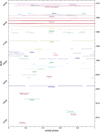 |
Fig. A.1. X-ray observations of Vela X-1 as reported in the literature and listed in Table A.1. |
| In the text | |
Current usage metrics show cumulative count of Article Views (full-text article views including HTML views, PDF and ePub downloads, according to the available data) and Abstracts Views on Vision4Press platform.
Data correspond to usage on the plateform after 2015. The current usage metrics is available 48-96 hours after online publication and is updated daily on week days.
Initial download of the metrics may take a while.