| Issue |
A&A
Volume 692, December 2024
|
|
|---|---|---|
| Article Number | A188 | |
| Number of page(s) | 13 | |
| Section | Stellar structure and evolution | |
| DOI | https://doi.org/10.1051/0004-6361/202450168 | |
| Published online | 12 December 2024 | |
Variable structures in the stellar wind of the HMXB Vela X-1
1
cosine Measurement Systems, Warmonderweg 14, 2171 AH Sassenheim, The Netherlands
2
Huygens-Kamerlingh Onnes Laboratory, Leiden University, Postbus 9504, 2300 RA Leiden, The Netherlands
3
European Space Agency (ESA), European Space Astronomy Centre (ESAC), Camino Bajo del Castillo s/n, 28692 Villanueva de la Cañada, Madrid, Spain
4
Departamento de Física, Universidad de Santiago de Chile, Av. Victor Jara 3659, Santiago, Chile
5
Center for Interdisciplinary Research in Astrophysics and Space Exploration (CIRAS), USACH, Santiago, Chile
6
European Space Agency (ESA), European Space Research and Technology Centre (ESTEC), Keplerlaan 1, 2201 AZ Noordwijk, The Netherlands
7
Instituto de Física de Cantabria (CSIC-Universidad de Cantabria), E-39005 Santander, Spain
8
Department of Applied Physics and Astronomy, College of Sciences and Sharjah Academy for Astronomy Space Sciences, and Technology (SAASST), University of Sharjah, PO Box 27272 Sharjah, UAE
9
INAF – Osservatorio Astronomico di Roma, Via Frascati 33, I-00040 Monte Porzio Catone, (RM), Italy
10
Institut für Astronomie und Astrophysik, Universität Tübingen, Sand 1, 72076 Tübingen, Germany
⋆ Corresponding author; This email address is being protected from spambots. You need JavaScript enabled to view it.
Received:
28
March
2024
Accepted:
12
October
2024
Abstract
Context. Strong stellar winds are an important feature in wind-accreting high-mass X-ray binary (HMXB) systems. Exploring their structure provides valuable insights into stellar evolution and their influence on surrounding environments. However, the long-term evolution and temporal variability of these wind structures are not fully understood.
Aims. This work probes the archetypal wind-accreting HMXB Vela X-1 using the Monitor of All-sky X-ray Image (MAXI) instrument to study the orbit-to-orbit absorption variability in the 2 − 10 keV energy band across more than 14 years of observations. Additionally, the relationship between hardness ratio trends in different binary orbits and the spin state of the neutron star is investigated.
Methods. We calculated X-ray hardness ratios to track absorption variability, comparing flux changes across various energy bands, as the effect of absorption on the flux is energy-dependent. We assessed variability by comparing the hardness ratio trends in our sample of binary orbits to the long-term averaged hardness ratio evolution derived from all available MAXI data.
Results. Consistent with prior research, the long-term averaged hardness ratio evolution shows a stable pattern. However, the examination of individual binary orbits reveals a different hardness ratio evolution between consecutive orbits with no evident periodicity within the observed time span. We find that fewer than half of the inspected binary orbits align with the long-term averaged hardness evolution. Moreover, neutron star spin-up episodes exhibit more harder-than-average hardness trends compared to spin-down episodes, although their distributions overlap considerably.
Conclusions. The long-term averaged hardness ratio dispersion and evolution are consistent with absorption column densities reported in literature from short observations, indicating that a heterogeneous wind structure – from accretion wakes to individual wind clumps – likely drives these variations. The variability observed from orbit to orbit suggests that pointed X-ray observations provide limited insights into the overall behaviour of the wind structure. Furthermore, the link between the spin state of the neutron star and the variability in orbit-to-orbit hardness trends highlights the impact of accretion processes on absorption. This connection suggests varying accretion states influenced by fluctuations in stellar wind density.
Key words: binaries: eclipsing / stars: massive / stars: neutron / stars: winds / outflows
© The Authors 2024
 Open Access article, published by EDP Sciences, under the terms of the Creative Commons Attribution License (https://creativecommons.org/licenses/by/4.0), which permits unrestricted use, distribution, and reproduction in any medium, provided the original work is properly cited.
This article is published in open access under the Subscribe to Open model. This email address is being protected from spambots. You need JavaScript enabled to view it. to support open access publication.
1. Introduction
Vela X-1 (4U 0900−40) has been among the best-studied X-ray sources since its discovery in 1967 (Chodil et al. 1967). The system is an eclipsing high-mass X-ray binary (HMXB) composed of a B0.5 Ia donor star, HD 77581 (Hiltner et al. 1972) and an accreting neutron star with a pulse period of ∼283 s (McClintock et al. 1976) in a low eccentric orbit (e ∼ 0.0898) of ∼8.964 days (Kreykenbohm et al. 2008). The high inclination of > 73° (van Kerkwijk et al. 1995) leads to regular X-ray eclipses of the neutron star, resulting in reduced observed X-ray emission, particularly in the hard X-ray band, for nearly 20% of the orbit. The neutron star has a magnetic field of ∼2.6 × 10¹² G (Fürst et al. 2014). The proximity of the system,  kpc (Kretschmar et al. 2021), makes it one of the brightest X-ray objects in the sky despite its modest mean luminosity of 5 × 1036 erg s−1 (Fürst et al. 2010). The neutron star has an estimated mass of ∼1.7 − 2.1 M⊙ (Kretschmar et al. 2021) and the radius of HD 77581 is 30 R⊙ (van Kerkwijk et al. 1995). The mean orbital separation of ∼1.7 R⋆ (Quaintrell et al. 2003) causes the neutron star to be heavily embedded in the dense and line-driven wind of the companion, which has a mass loss rate of ∼10−6 M⊙ yr−1 (Giménez-García et al. 2016). A fraction of the wind material is accreted and channelled to the magnetic poles of the neutron star, feeding the X-ray emission. In Fig. 1, we represent the orbit of the neutron star around HD 77581 as seen from Earth. For a comprehensive overview, we refer to Kretschmar et al. (2021).
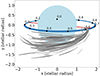 |
Fig. 1. Vela X-1 as seen from Earth, with an orbital inclination (i > 73°) compatible with the known constraints (with parameters from Kreykenbohm et al. 2008). The black points represent the positions of the neutron star at specific phases (with origin at the mid-eclipse time). The red line is the main axis of the eccentric orbit. Owing to the eccentricity, inferior conjunction of the neutron star occurs between ϕorb = 0.4 and ϕorb = 0.5. The accretion wake trailing the neutron star is represented at a fiducial orbital phase ϕorb = 0.6. |
HMXBs like Vela X-1 offer the opportunity to investigate both accretion onto compact objects, and the structure of winds from massive stars. To characterise the latter, we can use the neutron star as an X-ray probe orbiting in the wind and analyse the variability of the X-ray absorption along the line of sight. As commonly done in X-ray astronomy, we give the absorbing column, NH, in units of hydrogen atoms per cm2, and we assume a certain abundance of the heavier elements, such as O, S, Si, and Fe, relative to H. This abundance vector is based on the solar abundance given by Wilms et al. (2000). That is, the column is given as an equivalent hydrogen column, even though hydrogen does not contribute significantly to the absorption in the X-ray band. Understanding the structure and environmental impact of winds is important for studies of massive star evolution (Martínez-Núñez et al. 2017). The strong stellar winds produced by the donor stars are driven by line scattering of the star’s intense continuum radiation field (Lucy & Solomon 1970; Castor et al. 1975). Line-driven winds are unstable, with the line-deshadowing instability believed to be responsible for the formation of overdense inhomogeneities, or ‘clumps’, within a more diffuse plasma environment (Owocki & Rybicki 1984; Owocki et al. 1988; Feldmeier et al. 1995). In addition, large-scale structures are expected to form in the stellar wind due to the presence of the orbiting X-ray source influencing the wind flow via its gravity and the impact of the X-rays on the wind acceleration as further detailed below.
The accretion wake arises as a result of the wind-beaming induced by the gravitational field of the neutron star. This gravitational pull causes the stellar wind to be focused towards the neutron star, forming a concentrated flow that generates an unsteady bow shock in the vicinity of the neutron star (Blondin et al. 1991; Manousakis & Walter 2015a; Malacaria et al. 2016). The accretion wake is characterised by dynamic and evolving structures as the stellar wind interacts with the neutron star’s gravity. The photoionisation wake is generated by the X-ray radiation emitted by the neutron star. Similar to the concept of the Strömgen sphere around a blue star, iso-ξ surfaces are defined based on the ionisation parameter, ξ, around the neutron star (for more details, see e.g. Hatchett & McCray 1977; Manousakis & Walter 2015a,b; Sander et al. 2018). The X-ray radiation ionises the material within this region, forming a wake-like structure downstream of the neutron star. This photoionisation wake significantly influences the ionisation state and physical properties of the nearby gas (see e.g. Amato et al. 2021).
The intrinsic X-ray flux of Vela X-1 varies on a wide range of timescales. Similar to other X-ray pulsars, fluctuations within a pulse period are commonly observed (Staubert et al. 1980; Kretschmar et al. 2014). Vela X-1 also exhibits bright flares (Kreykenbohm et al. 2008; Martínez-Núñez et al. 2014; Lomaeva et al. 2020) and ‘off states’ on longer timesales (Inoue et al. 1984; Kreykenbohm et al. 1999, 2008; Doroshenko et al. 2011; Sidoli et al. 2015); in both cases, flux can quickly change by more than an order of magnitude. These variations are usually explained by enhanced accretion driven by instabilities at the outer rim of the neutron star magnetosphere. Overall, the flux variations have been found to follow a log-normal distribution (Fürst et al. 2010).
The X-ray spectrum of Vela X-1 outside eclipse resembles that of other accreting X-ray pulsars, characterized by a power-law shape with a high-energy turnover or cutoff, typically above 15−30 keV. This spectral profile is further modified by frequently strong absorption, an occasional added soft component, a prominent iron line, and cyclotron resonance scattering features in the hard X-rays (e.g. Haberl & White 1990; Kreykenbohm et al. 1999; Odaka et al. 2013; Fürst et al. 2014; Diez et al. 2022, 2023). The photon index of the power-law component exhibits mild variability, generally within a few percent, and shows a trend of spectral hardening with increasing brightness (Odaka et al. 2013; Fürst et al. 2014). In some studies (Martínez-Núñez et al. 2014; Malacaria et al. 2016), the power-law index is constant when a complex absorption component is included. However, in studies that allow for variations in the power-law index, changes in spectral hardness are mostly attributed to changes in the derived absorption (Haberl & White 1990; Diez et al. 2023).
The origin of this variable absorption is likely twofold. Given the high inclination of Vela X-1, the accretion wake is expected to intercept the line of sight as the neutron star orbits its stellar companion. The presence of the accretion wake from one orbit to another leads to a pattern in the orbital profile of NH where absorption is generally higher (lower) when the neutron star moves away from us (towards us), in agreement with the predictions from Manousakis & Walter (2015b). However, the absorption derived at the same orbital phase can be very different in observations taken during different orbits, indicating variable absorbing structures between individual binary orbits (Kretschmar et al. 2021, see also our Fig. 8). This effect is generally ascribed to unaccreted clumps in the wind that serendipitously intercept the line of sight, leading to an increase in NH on timescales of minutes to hours (Grinberg et al. 2017; El Mellah et al. 2020; Diez et al. 2022). To separate these two absorbing components, we need to monitor absorption variations over many orbits. The Monitor of All-sky X-ray Image (MAXI) instrument is particularly well suited for this task due to its continuous coverage of the entire orbit, enabling the study of orbit-to-orbit absorption variability that pointed X-ray observations, which cover only a small fraction of a single orbit, cannot provide.
The spin period of the neutron star in Vela X-1 has been monitored over decades, revealing periods of spinning up and down that can last for months. These variations may be linked to episodes of enhanced accretion. This is supported by studies such as that of OAO 1657−415, where fluorescence lines suggest that stochastic increases in absorption might be associated with enhanced accretion episodes (Pradhan et al. 2019). Changes in the spin state of the neutron star have been connected to the accreted material, though the exact mechanisms are not fully understood (Bozzo et al. 2008). Liao et al. (2022) report a positive correlation between spin-up events and the absorbing column density, and attribute it to episodes of increased mass loss from the donor star. They propose that spin-up and spin-down periods correspond to prograde and retrograde orbits of the accretion disk, respectively. However, this scenario is challenged by the absence of observed global variations in line-driven winds from massive stars, except in co-rotating interaction regions (Lobel & Blomme 2008). Additionally, the traditional model of accretion-induced torques, which involves coupling between a truncated accretion disk and a neutron star’s magnetosphere (Ghosh & Lamb 1979), is questioned in the context of Vela X-1 (Kretschmar et al. 2021). Alternative mechanisms that produce both positive and negative torques based on the angular momentum of the accretion flow have been suggested (Shakura et al. 2012).
In this study, we used MAXI to continuously monitor Vela X-1 to probe the variable structures in the stellar wind of the system. In particular, we focused on assessing the orbit-to-orbit absorption variability and investigating the spin state connection. Our research enhances studies conducted with pointed X-ray observations, which only cover a fraction of a single orbit. It should be noted that MAXI data only allow for the construction of detailed spectra when integrated over long time periods, as demonstrated in Malacaria et al. (2016) and Liao et al. (2022). Therefore, only hardness ratios are discussed. We demonstrate the impact of varying absorption in Fig. 2, which displays four different X-ray spectra taken by XMM-Newton, along with the corresponding absorbing column densities derived by Diez et al. (2023). Periods of high absorption (NH ≳ 20 × 1022 cm−2) lead to a substantial reduction in flux, particularly in the 2−4 keV band. These periods also reveal strong and ionised emission lines that can dominate the spectrum at lower energies. However, these lines mainly appear outside the energy range covered by the MAXI instrument and employed in this work (Watanabe et al. 2006). Moreover, the methodology presented in this work can be used to investigate similar HMXB systems. The instrument and dataset are described in Sect. 2. Our methods and data analysis are explained in Sects. 3 and 4. Finally, we discuss our results in Sect. 5 and provide a comprehensive summary of our findings and outline future prospects in Sect. 6.
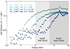 |
Fig. 2. Four unfolded spectra of Vela X-1 from XMM-Newton observation (2019) taken with EPIC-pn. Each spectrum is ∼283 s and corresponds to a different absorption column density value, from low NH (light green) to high NH (dark blue). The observation covers the 0.37−0.51 orbital phase range (Diez et al. 2023). The shaded zones cover the MAXI/GSC energy bands chosen for our analysis (2−4 keV and 4−10 keV). |
2. MAXI observations
2.1. MAXI
Vela X-1 is regularly monitored through MAXI (Matsuoka et al. 2009). This instrument is positioned on the International Space Station (ISS) within the Japanese Experiment Module and initiated its nominal observations in August 2009. It incorporates two types of X-ray slit cameras working in complementary ways: the Solid-State Slit Camera (SSC; Tomida et al. 2011) operating within the energy range of 0.5−12 keV, and the Gas Slit Camera (GSC; Mihara et al. 2011) in the 2−30 keV energy band.
We employed the MAXI/GSC in our study, which consists of six slit camera units, each housing two Xe-gas proportional counters equipped with 1D slit-slat collimators. The field of view is 1.5° ×160°, limited by the ISS structure and solar paddle. The 12 gas counters achieve a total detector area of 5350 cm2. The instrument has an all-sky coverage of ∼85% per ISS orbit and ∼95% per day. It scans a point source from 40 to 150 s, contingent upon the source incident angle Sugizaki et al. (2011).
2.2. Dataset
We used the ISS orbit light curve data1 to access the most detailed temporal information available over more than 14 years of MAXI observations as provided by the MAXI team (see Table 1).
MAXI dataset of Vela X-1.
The light curve data are available in three energy bands: 2−4 keV, 4−10 keV and 10−20 keV. The source fluxes provided assumed photon fluxes calculated under the assumption of a Crab-like spectrum (count rates), where the 2−20 keV value typically differs from the sum of the three individual bands. For simplicity, we henceforth use the term flux to refer to the corrected MAXI photon flux under the assumption of a Crab-like spectrum.
The dataset includes flare-like profiles due to unexpected background increases and dip-like profiles caused by the shadow effects of solar panels2. Calibration methods also introduce variability in 2−4 keV keV flux measurements due to absorption effects, which can impact the accuracy of flux values in this energy range. Additionally, uneven coverage arises from factors such as the source’s proximity to the Sun and system maintenance downtime, affecting data availability for specific binary orbits.
3. Flux and hardness average trends
In this section, we first introduce some relevant definitions for the entirety of our analysis. Subsequently, we explain the determination of our average trends and describe their evolution throughout the orbital period. These curves not only provide valuable information about the large-scale structures, as we discuss in Sect. 5.2, but also serve as a reference for quantifying orbit-to-orbit variability (see Sect. 4).
3.1. Preliminary definitions
In the subsequent analysis, we designate the 2−4 keV energy range as the ‘soft band’ and the 4−10 keV range as the ‘hard band’. The impact of absorption on the expected fluxes in these adjacent bands is markedly different for the range in NH typical for Vela X-1, namely 1−100 × 1022 cm−2 (Kretschmar et al. 2021, Fig. 4a), where it mainly impacts low energies, as shown in Fig. 2. The orbital phases (ϕorb) are obtained with the ephemeris from Kreykenbohm et al. (2008). We employed the mid-eclipse time of 52974.227 ± 0.007 MJD as the phase zero, and 8.964357 ± 0.000029 day as the orbital period.
The hardness ratio of the selected soft and hard energy bands is used to quantify absorption variability effects. We defined the hardness ratio as
 (1)
(1)
where H and S represent the MAXI fluxes in hard and soft band, respectively.
Unlike the traditional eclipse definition spanning from orbital phases 0.89 to 0.1 (e.g. Kreykenbohm et al. 2008), our study finds a notable decrease in hard flux from phases 0.87 to 0.89, making it difficult to establish a hardness ratio. Previous studies have shown that the definition of orbital eclipse phases is energy-dependent (e.g. Fig. 3 in Falanga et al. 2015). As a consequence, we restricted our analysis to the orbital phase range [0.10, 0.86], which encompasses 53.9% of the total sample of soft and hard fluxes.
3.2. Average trend analysis
The average trends in Fig. 3 (right) are derived from the histograms shown in the left panels of the same figure. Each orbital phase bin is of a size of 0.01, and is fitted using a normalised Gaussian distribution and a constant term. Due to sparse counts in each phase bin, the use of Cash statistics (Cash 1979) ensures non-biased fitting. The 1σ uncertainties in the Gaussian parameters are derived through Markov chain Monte Carlo sampling. The peak of the Gaussian represents the mean hardness of the phase bin, and its standard deviation provides the 1σ uncertainty. The fitting results for all phase bins are displayed as a function of the orbital phase. Moreover, an eighth-degree polynomial is applied to capture the overarching pattern, providing an overview of the dataset’s average behaviour.
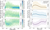 |
Fig. 3. Histograms and average trends of the MAXI/GSC dataset. Left: 2D histograms showing the unbinned MAXI/GSC dataset, depicting the flux in the 2−4 keV (soft band; top) and 4−10 keV energy range (hard band; middle), and the derived hardness ratio (bottom), calculated as explained in Sect. 3. The number of unbinned data points is colour-coded: lighter shades denote smaller values and darker shades indicate higher ones. Right: Average trends and their associated standard deviations derived from fits to the 2D histograms. Each shaded region is colour-coded, and the same code is used in Figs. 7 and B.1. For further details, we refer to the main text. |
To better understand the relative variability in each average trend curve across orbital phases, we computed the coefficient of variation (CV) by normalising each standard deviation (σ) to the associated mean value (μ) as follows:
 (2)
(2)
This metric enables direct comparisons across flux and hardness ratio curves, revealing variability patterns and trends relative to changes in their mean. In Fig. 4, we display the CV for the fluxes and hardness ratio curves from Fig. 3 (right panels). We refer to Sect. 3.3 for further details in the CV behaviour.
 |
Fig. 4. Coefficient of variation (CV; see Eq. (2)) of the flux and hardness average trends from Fig. 3 (right panels). |
3.3. Description of the flux and hardness average evolution
We observe a consistent decline with the orbital phase in both the soft and hard flux average trends (Figs. 3d, e), with a more significant decrease observed in the soft energy band. This is attributed to its heightened sensitivity to absorption effects, evidenced by an ∼90% decrease between the first and second halves of the orbital phase. The hard band is limited to the 4−10 keV energy range and is still noticeably affected by absorption (Fig. 2). The hardness average trend (Fig. 3f) exhibits lower hardness values in the first half compared to the second one.
While the flux mean decreases with the orbital phase, the associated standard deviation decreases less, causing the coefficient of variation (Eq. 2) to increase and eventually plateau after orbital phase 0.5 (Figs. 4a, b), indicating greater variability in the first half of the orbit. This is illustrated by the bump in the coefficient of variation of the hardness mean profile at orbital phases 0.2−0.4 (Fig. 4c). Further discussion on this topic can be found in Sect. 5.3.2.
4. Orbit-to-orbit variability in hardness profiles
In the following section, we analyse the variability of hardness ratios at the level of individual binary orbits, referred to hereafter as hardness profiles. First, we explain the construction of our sample of hardness profiles (Sect. 4.1). Thereafter, we describe the statistical method developed for the classification and quantification of the observed variability (Sect. 4.2).
4.1. Individual hardness profile sample selection
We began our analysis by extracting the flux outside the eclipse region to derive soft and hard fluxes binned per day, after which we computed hardness ratios. In Fig. B.1 we showcase an example of MAXI/GSC light curves, where median values are calculated within each time interval.
The investigation into orbit-to-orbit variability relies on hardness profiles with low uncertainties. Therefore, data points with uncertainties exceeding 0.4 are excluded. This criterion is informed by the uncertainty histogram depicted in Fig. 5. The histogram shows that imposing a stricter filter significantly diminishes the sample size without commensurately enhancing the accuracy of hardness ratios. This refinement process leads to a 42.0% reduction in the initial sample size.
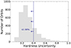 |
Fig. 5. Histogram of hardness uncertainties derived from fluxes outside the eclipse region, as defined in Sect. 3.1. The threshold, indicated by a vertical line refines the sample by excluding hardness values with uncertainties exceeding 0.4. See further details in Sect. 4.1. |
Lastly, to ensure sufficient information for assessing hardness variability in each binary orbit, we prioritised achieving adequate data coverage. Specifically, we referred to the system’s orbital period (Sect. 3.1) to guarantee a minimum of five 1-day-binned hardness values per orbit, capturing more than half of the maximum available information within each binary orbit. As a result, the final hardness profile sample size comprises 30.5% of the initial sample, totalling 315 orbital hardness profiles.
4.2. Deciphering orbit-to-orbit variability
The quantification of orbit-to-orbit hardness variability is not a trivial task due to the complex nature of the system. We quantify the relative variability of every hardness ratio value within every hardness profile (Sect. 4.2.1). Following this, we propose a criterion for classifying the evolution of hardness ratios in binary orbits (Sect. 4.2.2). Our statistical approach facilitates the understanding of individual hardness profiles, despite the resolution limitations of our dataset.
4.2.1. Quantifying relative variability using the complementary cumulative distribution function
The first step in the classification process involves evaluating every hardness ratio within each hardness profile, along with its corresponding uncertainty, relative to the hardness average trend. To achieve this, we utilised the cumulative distribution function (CDF), which describes the probability that a random variable takes on a value less than or equal to a specific value. In our context, taking their uncertainties into consideration helps determine how the observed hardness ratios compare to the average trend.
Treating the hardness ratio as the mean and its associated uncertainty as the 1σ standard deviation, we calculated the fraction of the Gaussian distribution (which represents the uncertainty in the hardness ratio) that lies above the hardness average trend by using the complementary CDF (i.e. 1−CDF). For example, hardness values with (1−CDF) values of 0.5 indicate that half of the Gaussian distribution is above the average trend. Conversely, (1−CDF) values close to 1 indicate that most of the distribution is above the average trend, while those nearing 0 indicate that most of the distribution is below the average trend.
4.2.2. Streamlined classification: Median of complementary CDF values for each hardness profile
After computing the (1−CDF) for each hardness ratio (Sect. 4.2.1), we calculated the median of these values within each hardness profile to establish the parameter F50, as follows:
 (3)
(3)
where N is the number of hardness ratios in the binary orbit, and (1−CDF) is the complementary CDF associated with each hardness ratio. We associated an F50 parameter with each binary orbit in our sample.
Then, we classified each hardness profile based on its F50 according to the following criteria: orbits with an F50 falling within 0.4 ≤ F50 ≤ 0.6 are classified as ‘standard’, while those with F50 > 0.6 are defined as ‘harder’ profiles, and those with F50 < 0.4 are categorised as ‘softer’ profiles. The F50 histogram of the analysed profiles is displayed in Fig. 6, depicting the defined thresholds of the criteria. This classification reveals that 42.8% of the orbits align with the mean profile and are classified as standard profiles, while 35.9% are softer, and 21.3% are harder profiles. The analysis of this distribution is further discussed in Sect. 5.3.3.
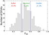 |
Fig. 6. Histogram of the F50 parameter (Eq. (3)) illustrating the streamlined classification as explained in Sect. 4.2.2, with vertical dashed blue lines indicating the defined thresholds for each type of hardness profile. We refer to the main text for further details. |
In Fig. 7 we show two representative hardness profile examples from each of the three categories. The left column displays hardness evolution patterns, which one would unequivocally classify visually in the same manner as our statistical criterion. However, the simplicity of our classification method is demonstrated by the hardness evolution patterns in the right column, where visual classification is less evident.
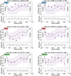 |
Fig. 7. Orbit-to-orbit hardness profiles categorised into three groups based on F50 thresholds (Eq. (3)): harder (F50 > 0.6, top, blue), softer (F50 < 0.4, middle, red), and standard (0.4 ≥ F50 ≥ 0.6, bottom, green). Left column: Well-defined orbits. Right column: Orbits from the same group with larger variability (see Appendix A for a more elaborated statistical analysis derived from the analysis outlined in Sect. 4.2.2). We refer to the main text for further details. |
In Appendix A we elaborate on our approach to quantifying variability using the three-group classification based on the F50 parameter (Eq. (3)). This method measures the magnitude and direction of outliers from the overall evolution for each hardness profile, providing a visual and comprehensive description of the hardness ratio evolution in each binary orbit without the need for individual sample inspection (Fig. A.1).
5. Discussion
In Sect. 3, we describe the Vela X-1 long-term evolution, revealing persistent patterns over more than 14 years of continuous MAXI monitoring (as also found by several previous studies). However, significant variability in X-ray absorption is still evident (Fig. 3). The fluctuations in the hardness ratio are most pronounced during periods of low absorption between orbital phases 0.2 and 0.4 (Fig. 4), but also occasionally high NH (Fig. 8). This section discusses explanations for the absorption variability for individual binary orbits. Additionally, we discuss the connection between the spin state and orbit-to-orbit absorption variability.
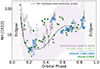 |
Fig. 8. Absorption column density values across the orbital phase derived from multiple X-ray satellite observations adapted from Kretschmar et al. (2021). We refer to the main text for considerations when comparing absolute NH values. Different symbols are used to show data taken in different binary orbits by the same mission. The mean hardness profile from our MAXI/GSC sample is visually scaled and superimposed. The hardness ratio correlates positively with NH but lacks a direct one-to-one relationship, hence the need for an arbitrary scaling. |
5.1. Hardness as a diagnostic for tracing absorption variability
To justify the use of hardness ratios and demonstrate their sensitivity to variations in NH, we simulated spectra based on the best-fit model described in Diez et al. (2023), covering the range of spectral slopes observed in their study. Assuming minimal absorption, when the continuum slope has the most significant effect, the hardness ratio difference between photon index extremes (0.8 and 1.2) is only ∼0.13. Conversely, assuming the hardest continuum, where NH has the least impact on the hardness ratio, and varying NH, the difference exceeds 0.5. For all other cases the slope’s impact is even less significant, indicating that absorption variations primarily dominate the observed hardness ratios.
Variations in the amount of absorbing material due to the non-uniform stellar wind or the accretion wake structure cause significant energy-dependent flux changes in the energy bands covered by MAXI (Sect. 1 and Fig. 2), leading to noticeable hardness ratio variations and allowing us to use hardness ratio variations as a proxy for absorption changes.
In the analysis, the changing ionisation structure of the wind, particularly during flares, is addressed by considering the variability in the ionisation parameter, ξ, which is influenced by X-ray luminosity (LX), distance from the neutron star, and local number density. Simulations assume a constant LX, resulting in ξ primarily depending on distance and density. Flares, which last for thousands of seconds and can increase LX by a factor of 3−4 and more, can disrupt this assumption as the ionisation parameter and the local density can fluctuate substantially. However, the time resolution of MAXI, which provides a ∼90-second snapshot every ∼90 minutes, limits the ability to capture these rapid changes. As flares are often longer than the MAXI sampling interval, they introduce scatter in the average measurements rather than detailed temporal profiles. This means that the variations in ionisation due to flares are averaged out in the analysis, contributing to the observed scatter in the hardness ratio.
Our study focuses on changes within individual binary orbits. In Fig. 8, we compare the long-term average hardness ratio trend from our MAXI/GSC sample (Fig. 3f) with NH values obtained by various X-ray observatories. The average hardness trend has been arbitrarily scaled to facilitate comparison and emphasise similarity in overall trend. Direct comparisons of absolute NH values from various studies should be approached cautiously, given distinct models and assumptions in the literature. Nonetheless, Fig. 8 illustrates the variability in NH measurements obtained through pointed X-ray observations at comparable orbital phases over different time periods. The close correspondence between our average hardness profile as a function of orbital phase and the literature measurements shows that monitoring over multiple orbits is necessary to properly track the evolution of the absorption components.
5.2. Large-scale steady structures
The mean hardness profile (Fig. 3f) reveals an asymmetry between the first and second halves of the orbital period, suggesting the presence of large-scale structures, such as an accretion wake trailing the neutron star. The wake structure is attributed to the gravitational and radiative impacts of the neutron star on the outflowing stellar wind (see Kretschmar et al. 2021). The soft flux average trend reveals a significant reduction of ∼90% between the first and second halves of the orbit, coinciding with the presence of the wake structure in the line of sight. A similar trend is observed in the average profile of the hard flux (Fig. 3e), though it is less pronounced since the hard flux band is less affected by absorption. Early studies by Bessell et al. (1975) and subsequent simulations by Blondin et al. (1991) and Manousakis et al. (2012) highlight the persistent trailing of this wake throughout the neutron star’s orbit.
During the eclipse egress, occurring at orbital phases 0.1−0.2, there is a rapid decrease in the hardness ratio, also indicated by the NH values in Fig. 8. This decline is typically linked to the presence of the extended stellar atmosphere obscuring the line of sight (Sato et al. 1986; Lewis et al. 1992). Next, a plateau emerges at orbital phases 0.2−0.4. This likely arises from the wake structure positioned away from our line of sight such that our line of sight intersects a wind region of lower density leading to lower observed hardness values.
Thereafter, the average hardness smoothly increases between orbital phases 0.4 to 0.6. Prior observational results and theoretical models show steep increases for individual orbits: Ohashi et al. (1984), using Tenma data, finds that the NH steeply increases within this phase interval (Fig. 8). Diez et al. (2023) analyse an XMM-Newton observation spanning orbital phases 0.34−0.48 (Fig. 8) and show a steep increase, but at a slightly different point in the orbit. Similarly, Manousakis et al. (2012) predict a model with a similar steep absorption increase, although it was developed for a different system with similar system parameters. The smooth continuous trend observed with MAXI during these orbital phases can then be attributed to variations in the onset timing of absorption increase across different orbits, resulting in an overall smoother average transition.
A second plateau with sustained higher hardness values is observed from 0.6 to 0.8, attributed to our line of sight intersecting the wake. However, during this second plateau, the hardness average trend shows a slight decrease due to the interplay of two phenomena: the trailing wake structure begins to move out of our line of sight, resulting in less material absorbing the X-ray emission of the neutron star and simultaneously, the extended stellar atmosphere of the companion starts absorbing the X-ray emission. The decrease caused by the displacement of the wake structure is partially counteracted by the onset of eclipse ingress. However, it is only after phase 0.8 that the absorption levels of the eclipse ingress are sufficiently high to produce a similar rapid absorption increase, mirroring the eclipse egress behaviour.
5.3. Stochastic variations in absorption
The dynamic interaction among the different components of the Vela X-1 system, including the neutron star, the stellar wind, and the accretion wake results in stochastic fluctuations observed in X-rays. First, we examine the origins of this stochastic variability based on literature (Sect. 5.3.1). We then deduce it through the analysis of MAXI long-term average trends (Sect. 5.3.2), as well as from individual hardness profiles (Sect. 5.3.3).
5.3.1. Previous observational results and model descriptions
Multiple components can contribute to the stochastic variability, such as variations in material integration along the line of sight induced by clumps in the stellar wind, accumulation of matter and modifications of the flow geometry at the outer rim of the neutron star magnetosphere, or changes in opacity due to changes in wind ionisation structure.
Wind clumps crossing the line of sight can cause short-timescale absorption variability. The 2D model from Oskinova et al. (2012) considers massive and intermediate-sized overdense shells propagating radially from the donor star. They compute the time-dependent extinction coefficient, revealing that radially compressed clumps exhibit greater variability than their spherical counterparts. El Mellah et al. (2020) expand on this by modelling column density variability from spherical clumps using a 3D model of radial clump flow, computing median NH profiles and standard deviations across multiple orbits. They find that NH varies on the flyby timescale of the smallest clumps, allowing estimates of their size and mass based on column density standard deviation.
Changes in the flow structure near the neutron star’s magnetosphere contribute to the formation of wakes, which in turn affect the variability of absorption along the line of sight. However, the size of the wake structure exceeds not only the orbital separation between the neutron star and its donor, but also significantly surpasses the size of the neutron star’s magnetosphere (Kretschmar et al. 2021, Fig. 2). Consequently, while flow structure changes do play a role in stochastic absorption variability, their impact is minor. The smooth stellar wind dynamics in hydrodynamics numerical simulations by Manousakis & Walter (2011) successfully replicate the column density excesses observed in the orbital phases 0.4−0.8, attributing them to an overdense accretion wake trailing the neutron star. Malacaria et al. (2016) demonstrate the inhomogeneous nature of this wake structure through detailed spectral analysis of enhanced absorption events near inferior conjunction, in agreement with Doroshenko et al. (2013).
In the vicinity of the neutron star, extending from the magnetosphere to regions approximately 100 times farther, intrinsic variations in X-ray ionising emissions influence the structure of the stellar wind (Kretschmar et al. 2021, Fig. 2). In highly ionised regions, particularly those near the neutron star or in low-density areas, X-rays can pass through with minimal absorption. Consequently, fluctuations in the wind’s ionisation state can lead to observed variations in the column density, even if the actual amount of absorbing material along the line of sight remains constant.
In the vicinity of the neutron star, ranging from the magnetosphere to distances larger by about two orders of magnitude but still small on the system scale (Kretschmar et al. 2021, Fig. 2), intrinsic variations in X-ray ionising emissions influence the structure of the stellar wind. The regions of the wind that are highly ionised, particularly those near the neutron star and in regions of low density, permit X-rays to pass through without affecting the observed absorption column density. Thus, even with no change in the amount of material along the line of sight, these fluctuations in the wind’s ionisation state can lead to observed variation in the absorbing column density.
5.3.2. Stochastic variability inferred from the MAXI long-term average profile
The analysis of the mean profiles of both flux and hardness ratio together with their coefficient of variation (Sect. 3.3) reveals the stochastic nature of the system.
The bump observed in the coefficient of variation of the hardness ratio (Fig. 4c) between orbital phases 0.2 and 0.4, with an increase of approximately 50%, coincides with the absence of the wake structure in the line of sight. During this phase, irregular absorption variability caused by stellar clumps becomes more significant, leading to a peak in variability. This is consistent with historically reported absorption column density values (Fig. 8), which show greater scatter in NH values during the first half of the orbit.
Following mid-orbit, a major wake structure consistently obstructs the line of sight, regardless of individual variations (Sect. 5.2). During these orbital phases, the absorption variability derived from the average trends is reduced, as the individual contributions from different binary orbits are smoothed out by the wake structure, which serves as the primary contributor to absorption.
The rapid decrease in the hardness average trend observed during eclipse egress (Fig. 3f) is largely attributed to the influence of the extended stellar atmosphere (Sect. 5.2) and shows low variability (Fig. 4c). However, previous studies (Puls et al. 2006; Cohen et al. 2011; Torrejón et al. 2015) have identified significant clumping near the photosphere of OB stars. The impact of this clumping on absorption changes during eclipse egress remains uncertain, as such changes coincide with the rapid movement of the line of sight away from the star.
5.3.3. Stochastic variability inferred from MAXI binary orbits
Our three-category classification (Sect. 4.2.2) enables a systematic assessment of absorption variability at the level of individual binary orbits. However, the dynamics of the system necessitate a more sophisticated statistical approach to quantifying the observed fluctuations (Appendix A).
Vela X-1 displays a standard hardness profile in ∼40% of cases (Fig. 6). However, we find a considerable number of hardness profiles in this category that deviate from the average hardness evolution but are within the ±20% of the average trend. Thus, fewer than 40% of pointed X-ray observations will encounter conditions that deviate significantly from the average orbit. We refer to Kretschmar et al. (2021, Fig. A.1 and Table A.1) for a discussion of X-ray observations of Vela X-1 reported in the literature.
The remainder of our sample displays either softer hardness profiles with consistently lower absorption levels throughout the orbital period or harder profiles characterised by higher absorption levels (Fig. 6). These absorption profiles are influenced by factors such as the clumpy nature of the stellar wind and inherent variability of the source. Additionally, inspection of individual binary orbits reveals increased absorption occurring at earlier orbital phases before 0.4, when the wake structure crosses the line of sight. The onset of the wake structure does not consistently occur at the exact same orbital phase across different binary orbits, but fluctuates around ∼0.4 due to wake structure turbulence. This variability explains the smooth increase observed in the long-term average trend of the hardness ratio (Fig. 3f) towards higher absorption values during the latter half of the orbit.
Overall, the hardness profiles exhibit variability from one orbit to the next, and no periodicities are found in the 14 years of MAXI observations.
5.4. The link between spin variations and X-ray absorption
The continuous monitoring of the neutron star’s spin period over the past decades has revealed discernible phases characterised by steady increases and decreases in rotation rates over weeks to months (Malacaria et al. 2020). However, these fluctuations have exhibited an overall negligible net impact over the past four decades when compared to local deviations (Fürst et al. 2010). In contrast to glitches observed in radio pulsars, the alterations in spin periods of neutron stars in X-ray binaries are believed to arise from accretion-induced torques, in particular in Vela X-1 where the stellar wind captured by the neutron star has enough angular momentum to circularise before it reaches the magnetosphere (El Mellah et al. 2019). This hypothesis implies a dependence on the mass accretion rate, specifically on the quantity of plasma surrounding the neutron star and capable of absorbing X-ray emissions from its magnetic poles. Consequently, spin-up periods would be characterised by higher X-ray hardness (i.e. periods of higher accretion).
We investigated this hypothesis by combining our sample with the time series of the neutron star spin period from Liao et al. (2022, Fig. 1), who examined spectral properties, column densities, and Swift/BAT flux orbital profiles during spin-up and spin-down episodes. We selected MAXI binary orbits from our sample (Sect. 4.1) based on their spin intervals, resulting in 44 binary orbits classified as spin-up and 37 as spin-down.
The mean of the 1-day binned hardness values from the selected binary orbits is calculated separately for spin-up and spin-down states, resulting in 0.453 ± 0.012 and 0.384 ± 0.013, respectively. We used a Kolmogorov-Smirnov test to confirm that the difference in mean hardness values between the two spin groups is statistically significant. According to our criteria to quantify hardness ratio variability (Sect. 4.2), the prevalence of harder-than-average hardness profiles in the spin-up group is higher compared to the spin-down group by a factor of ∼5. We ascribe the hardness increases to enhanced X-ray absorption along the line of sight, meaning that the neutron star is engulfed in a higher amount of absorbing material when it spins-up. This is despite the higher X-ray ionising flux from the neutron star during spin-up events, for which Liao et al. (2022) found that the 15−50 keV Swift/BAT flux was on average ∼1.6 times higher than during spin-down events. The overall increase in hardness indicates that most of the absorbing material will be at distances from the neutron star where the ionisation parameter is too low to have a significant impact, in line with the predicted large structures. However, there is substantial scatter in both groups: some spin-up (spin-down) episodes are associated with softer-than-average (harder-than-average) emission, and when examining hardness evolutions at the level of individual binary orbits, no clear distinction is apparent.
Liao et al. (2022) suggest that spin-up (spin-down) could be induced by a prograde (retrograde) disk, with disk rotation switches controlled by stellar wind variations over tens of days. However, line-driven winds from massive stars do not show periodic variations on these timescales, and it is unclear whether enhanced stellar mass loss is due to changes in wind speed and/or density. While wind density changes would not affect the specific angular momentum of the accreted flow, slower winds lead to a prograde disk, while faster winds lower the circularisation radius below the magnetosphere radius, resulting in quasi-spherical accretion (El Mellah & Casse 2017). Stochastic variations could still temporarily form a prograde or retrograde disk, but clumps are too small to match the required scales (Sundqvist et al. 2018).
Spinning-down accretion-induced torques do not necessarily require retrograde disks: they can be achieved either through a magneto-centrifugal gating mechanism commonly called the propeller regime (Bozzo et al. 2008), or through quasi-spherical subsonic accretion (Shakura et al. 2012). The propeller regime is triggered when the magnetosphere radius (which is close to the inner edge of the disk) is larger than the co-rotation radius. The plasma at the inner edge of the accretion disk has to spin up in order to couple to the dipolar magnetic field lines in solid rotation with the neutron star. Therefore, the plasma experiences an additional centrifugal force which can lead to its ejection, or at least halt its penetration into the neutron star magnetosphere. Alternatively, in the quasi-spherical subsonic accretion model, the plasma does not have enough angular momentum to form a disk. Instead, it settles down on the neutron star magnetosphere as an extended quasi-static shell. The accretion into the magnetosphere is mediated by Compton cooling and convective motions in the shell.
Our interpretation for the observed episodes of spin-up and spin-down is based on these two models. The serendipitous capture of a wind clump or a temporary increase in the overall stellar wind density could trigger transitions between the propeller regime – where the neutron star is spun down as plasma accumulates at the outer rim of its magnetosphere – and a regime of direct accretion, where accretion-induced torques spin up the neutron star. Yet, the absence of correlation between the sign of the accretion-induced torque and the X-ray flux indicates that the propeller is not enough to explain the behaviour of the neutron star spin. Instead, we speculate that the capture of a clump can significantly lower the specific angular momentum of the flow and temporarily bring the system in the quasi-spherical subsonic configuration. In this case, positive and negative torques can be produced independently of the X-ray flux. More importantly, the spin-up episode can be sustained as long as the reservoir of plasma that was present at the outer rim of the neutron star magnetosphere contains enough material. Therefore, it lasts much longer (typically a few weeks) than the stellar wind variation that triggered it, be it clump capture or enhanced wind density. This interpretation accounts for the predominance of higher X-ray hardness ratios during the spin-up episodes. Also, it would explain why we observe such a huge scatter around the aforementioned hardness ratios mean values: even when wind density at the orbital scale comes back to its standard values, the spin-up episodes continue.
6. Conclusion and outlook
In this study, we conducted a comprehensive analysis of the long-term evolution and variability of X-ray absorption in the wind-accreting HMXB Vela X-1 using all-sky monitor MAXI data. We demonstrate that NH is the primary factor influencing changes in the hardness ratio and utilise it as a tracer of absorption variability. This technique enables the analysis of absorption-induced variations across the entire orbital period.
The novelty of this work lies in the investigation of absorption variability within individual binary orbits over 14 years of continuous observations. Our principal findings are:
-
Large-scale structures, such as the accretion wake trailing the neutron star, significantly influence the observed absorption patterns, consistent with existing literature on the impact of hydrodynamic interactions between the neutron star and the stellar wind.
-
There is significant variability in hardness profiles from one orbit to the next, without any discernible periodic pattern. This variability underscores the heterogeneous composition of wind structures. The stochastic variability of absorption, mainly attributed to clumps in the stellar wind, contributes to short-term absorption variations.
-
Fewer than 40% of the hardness profiles follow a typical hardness evolution within a 20% difference from the average trend. Therefore, pointed X-ray observations are likely to encounter non-average scenarios, explaining the diversity of NH values observed at the same orbital phase in the literature.
-
Spin-up events in Vela X-1 correlate positively with harder-than-average binary orbits, reflecting increased absorption along the line of sight; this indicates a higher density of surrounding absorbing material. The observed spin variations are attributed to accretion-induced torques, with spin-up episodes sustained by a reservoir of plasma around the neutron star’s magnetosphere. This suggests an interplay between the accreted plasma, variations in the stellar wind from the donor star, and the neutron star’s magnetosphere.
The statistical approach followed in this study demonstrates its applicability to other similar sources monitored by MAXI, suggesting its potential for broader usage in understanding absorption variability in binary systems. Our findings suggest the need for an increase in the number of modelled orbits used in theoretical studies to better capture the observed absorption dynamics in binary systems.
Moreover, the enhanced sensitivity of the upcoming Einstein Probe mission (Yuan et al. 2022) holds promise for conducting similar studies with greater detail. Its improved capabilities compared to current observatories will enable a deeper exploration of the complexities of X-ray absorption variability, providing further insights into the dynamics of stellar winds and processes of accretion onto neutron stars.
MAXI dataset employed for the analysis available at: http://maxi.riken.jp/star_data/J0902-405/J0902-405.html
MAXI Readme: http://maxi.riken.jp/top/readme.html
Acknowledgments
We thank the anonymous referee, who has improved the clarity of this manuscript. LA acknowledges the support by cosine measurement systems, and SMN acknowledges funding under project PID2021-122955OB-C41 funded by MCIN/AEI/10.13039/501100011033 and by ‘ERDF A way of making Europe’. We acknowledge support from ESA through the Science Faculty – Funding reference ESA-SCI-SC-LE-181, the Institute of Space Science (ICE) – CSIC, and the Institut d’Estudis Espacials de Catalunya (IEEC). This research was supported by the International Space Science Institute (ISSI) in Bern, through ISSI International Team project #495 (Feeding the spinning top). We thank Zhenxuan Liao’s team at Sanming University in China for sharing the time intervals in the spin frequency history used in their research. This research has made use of (1) the MAXI data provided by RIKEN, JAXA, and the MAXI team; (2) the Interactive Spectral Interpretation System (ISIS) (Houck & Denicola 2000; Houck 2002; Noble & Nowak 2008) maintained by the Chandra X-ray Center group at MIT; (3) the ISIS function (isisscripts) (http://www.sternwarte.uni-erlangen.de/isis/) provided by ECAP/Remeis observatory and MIT; (4) NASA’s Astrophysics Data System Bibliographic Service (ADS); (5) the Astropy package (https://www.astropy.org/) (Astropy Collaboration 2013, 2018) and Matplotlib library (https://matplotlib.org/) (Hunter 2007) for data analysis and visualisation.
References
- Amato, R., Grinberg, V., Hell, N., et al. 2021, A&A, 648, A105 [NASA ADS] [CrossRef] [EDP Sciences] [Google Scholar]
- Astropy Collaboration (Robitaille, T. P., et al.) 2013, A&A, 558, A33 [NASA ADS] [CrossRef] [EDP Sciences] [Google Scholar]
- Astropy Collaboration (Price-Whelan, A. M., et al.) 2018, AJ, 156, 123 [Google Scholar]
- Bessell, M. S., Vidal, N. V., & Wickramasinghe, D. T. 1975, ApJ, 195, L117 [NASA ADS] [CrossRef] [Google Scholar]
- Blondin, J. M., Stevens, I. R., & Kallman, T. R. 1991, ApJ, 371, 684 [NASA ADS] [CrossRef] [Google Scholar]
- Bozzo, E., Falanga, M., & Stella, L. 2008, ApJ, 683, 1031 [Google Scholar]
- Cash, W. 1979, ApJ, 228, 939 [Google Scholar]
- Castor, J. I., Abbott, D. C., & Klein, R. I. 1975, ApJ, 195, 157 [Google Scholar]
- Chodil, G., Mark, H., Rodrigues, R., Seward, F. D., & Swift, C. D. 1967, ApJ, 150, 57 [NASA ADS] [CrossRef] [Google Scholar]
- Cohen, D. H., Gagné, M., Leutenegger, M. A., et al. 2011, MNRAS, 415, 3354 [NASA ADS] [CrossRef] [Google Scholar]
- Diez, C. M., Grinberg, V., Fürst, F., et al. 2022, A&A, 660, A19 [NASA ADS] [CrossRef] [EDP Sciences] [Google Scholar]
- Diez, C. M., Grinberg, V., Fürst, F., et al. 2023, A&A, 674, A147 [NASA ADS] [CrossRef] [EDP Sciences] [Google Scholar]
- Doroshenko, V., Santangelo, A., & Suleimanov, V. 2011, A&A, 529, A52 [NASA ADS] [CrossRef] [EDP Sciences] [Google Scholar]
- Doroshenko, V., Santangelo, A., Nakahira, S., et al. 2013, A&A, 554, A37 [NASA ADS] [CrossRef] [EDP Sciences] [Google Scholar]
- El Mellah, I., & Casse, F. 2017, MNRAS, 467, 2585 [NASA ADS] [Google Scholar]
- El Mellah, I., Sander, A. A. C., Sundqvist, J. O., & Keppens, R. 2019, A&A, 622, A189 [NASA ADS] [CrossRef] [EDP Sciences] [Google Scholar]
- El Mellah, I., Grinberg, V., Sundqvist, J. O., Driessen, F. A., & Leutenegger, M. A. 2020, A&A, 643, A9 [NASA ADS] [CrossRef] [EDP Sciences] [Google Scholar]
- Falanga, M., Bozzo, E., Lutovinov, A., et al. 2015, A&A, 577, A130 [NASA ADS] [CrossRef] [EDP Sciences] [Google Scholar]
- Feldmeier, A., Puls, J., Reile, C., et al. 1995, Ap&SS, 233, 293 [Google Scholar]
- Fürst, F., Kreykenbohm, I., Pottschmidt, K., et al. 2010, A&A, 519, A37 [CrossRef] [EDP Sciences] [Google Scholar]
- Fürst, F., Pottschmidt, K., Wilms, J., et al. 2014, ApJ, 780, 133 [Google Scholar]
- Ghosh, P., & Lamb, F. K. 1979, ApJ, 234, 296 [Google Scholar]
- Giménez-García, A., Shenar, T., Torrejón, J. M., et al. 2016, A&A, 591, A26 [EDP Sciences] [Google Scholar]
- Grinberg, V., Hell, N., El Mellah, I., et al. 2017, A&A, 608, A143 [NASA ADS] [CrossRef] [EDP Sciences] [Google Scholar]
- Haberl, F., & White, N. E. 1990, ApJ, 361, 225 [Google Scholar]
- Hatchett, S., & McCray, R. 1977, ApJ, 211, 552 [NASA ADS] [CrossRef] [Google Scholar]
- Hiltner, W. A., Werner, J., & Osmer, P. 1972, ApJ, 175, L19 [Google Scholar]
- Houck, J. C. 2002, in High Resolution X-ray Spectroscopy with XMM-Newton and Chandra, ed. G. Branduardi-Raymont, 17 [Google Scholar]
- Houck, J. C., & Denicola, L. A. 2000, ASP Conf. Ser., 216, 591 [Google Scholar]
- Hunter, J. D. 2007, Comput. Sci. Eng., 9, 90 [NASA ADS] [CrossRef] [Google Scholar]
- Inoue, H., Ogawara, Y., Ohashi, T., et al. 1984, PASJ, 36, 709 [Google Scholar]
- Kretschmar, P., Marcu, D., Kühnel, M., et al. 2014, Eur. Phys. J. Web Conf., 64, 06012 [NASA ADS] [CrossRef] [EDP Sciences] [Google Scholar]
- Kretschmar, P., El Mellah, I., Martínez-Núñez, S., et al. 2021, A&A, 652, A95 [NASA ADS] [CrossRef] [EDP Sciences] [Google Scholar]
- Kreykenbohm, I., Kretschmar, P., Wilms, J., et al. 1999, A&A, 341, 141 [NASA ADS] [Google Scholar]
- Kreykenbohm, I., Wilms, J., Kretschmar, P., et al. 2008, A&A, 492, 511 [NASA ADS] [CrossRef] [EDP Sciences] [Google Scholar]
- Lewis, W., Rappaport, S., Levine, A., & Nagase, F. 1992, ApJ, 389, 665 [NASA ADS] [CrossRef] [Google Scholar]
- Liao, Z., Liu, J., & Gou, L. 2022, MNRAS, 517, L111 [NASA ADS] [CrossRef] [Google Scholar]
- Lobel, A., & Blomme, R. 2008, ApJ, 678, 408 [NASA ADS] [CrossRef] [Google Scholar]
- Lomaeva, M., Grinberg, V., Guainazzi, M., et al. 2020, A&A, 641, A144 [NASA ADS] [CrossRef] [EDP Sciences] [Google Scholar]
- Lucy, L. B., & Solomon, P. M. 1970, ApJ, 159, 879 [Google Scholar]
- Malacaria, C., Mihara, T., Santangelo, A., et al. 2016, A&A, 588, A100 [NASA ADS] [CrossRef] [EDP Sciences] [Google Scholar]
- Malacaria, C., Jenke, P., Roberts, O. J., et al. 2020, ApJ, 896, 90 [NASA ADS] [CrossRef] [Google Scholar]
- Manousakis, A., & Walter, R. 2011, A&A, 526, A62 [NASA ADS] [CrossRef] [EDP Sciences] [Google Scholar]
- Manousakis, A., & Walter, R. 2015a, A&A, 575, A58 [NASA ADS] [CrossRef] [EDP Sciences] [Google Scholar]
- Manousakis, A., & Walter, R. 2015b, A&A, 584, A25 [NASA ADS] [CrossRef] [EDP Sciences] [Google Scholar]
- Manousakis, A., Walter, R., & Blondin, J. M. 2012, A&A, 547, A20 [NASA ADS] [CrossRef] [EDP Sciences] [Google Scholar]
- Martínez-Núñez, S., Torrejón, J. M., Kühnel, M., et al. 2014, A&A, 563, A70 [NASA ADS] [CrossRef] [EDP Sciences] [Google Scholar]
- Martínez-Núñez, S., Kretschmar, P., Bozzo, E., et al. 2017, Space Sci. Rev., 212, 59 [Google Scholar]
- Matsuoka, M., Kawasaki, K., Ueno, S., et al. 2009, PASJ, 61, 999 [Google Scholar]
- McClintock, J. E., Rappaport, S., Joss, P. C., et al. 1976, ApJ, 206, L99 [Google Scholar]
- Mihara, T., Nakajima, M., Sugizaki, M., et al. 2011, PASJ, 63, S623 [Google Scholar]
- Noble, M. S., & Nowak, M. A. 2008, PASP, 120, 821 [Google Scholar]
- Odaka, H., Khangulyan, D., Tanaka, Y. T., et al. 2013, ApJ, 767, 70 [Google Scholar]
- Ohashi, T., Inoue, H., Koyama, K., et al. 1984, PASJ, 36, 699 [NASA ADS] [Google Scholar]
- Oskinova, L. M., Feldmeier, A., & Kretschmar, P. 2012, MNRAS, 421, 2820 [NASA ADS] [CrossRef] [Google Scholar]
- Owocki, S. P., & Rybicki, G. B. 1984, ApJ, 284, 337 [Google Scholar]
- Owocki, S. P., Castor, J. I., & Rybicki, G. B. 1988, ApJ, 335, 914 [NASA ADS] [CrossRef] [Google Scholar]
- Pradhan, P., Raman, G., & Paul, B. 2019, MNRAS, 483, 5687 [NASA ADS] [CrossRef] [Google Scholar]
- Puls, J., Markova, N., Scuderi, S., et al. 2006, A&A, 454, 625 [NASA ADS] [CrossRef] [EDP Sciences] [Google Scholar]
- Quaintrell, H., Norton, A. J., Ash, T. D. C., et al. 2003, A&A, 401, 313 [NASA ADS] [CrossRef] [EDP Sciences] [Google Scholar]
- Sander, A. A. C., Fürst, F., Kretschmar, P., et al. 2018, A&A, 610, A60 [NASA ADS] [CrossRef] [EDP Sciences] [Google Scholar]
- Sato, N., Hayakawa, S., Nagase, F., et al. 1986, PASJ, 38, 731 [NASA ADS] [Google Scholar]
- Shakura, N., Postnov, K., Kochetkova, A., & Hjalmarsdotter, L. 2012, MNRAS, 420, 216 [Google Scholar]
- Sidoli, L., Paizis, A., Fürst, F., et al. 2015, MNRAS, 447, 1299 [NASA ADS] [CrossRef] [Google Scholar]
- Staubert, R., Kendziorra, E., Pietsch, W., et al. 1980, ApJ, 239, 1010 [NASA ADS] [CrossRef] [Google Scholar]
- Sugizaki, M., Mihara, T., Serino, M., et al. 2011, PASJ, 63, S635 [Google Scholar]
- Sundqvist, J. O., Owocki, S. P., & Puls, J. 2018, A&A, 611, A17 [NASA ADS] [CrossRef] [EDP Sciences] [Google Scholar]
- Tomida, H., Tsunemi, H., Kimura, M., et al. 2011, PASJ, 63, 397 [NASA ADS] [Google Scholar]
- Torrejón, J. M., Schulz, N. S., Nowak, M. A., et al. 2015, ApJ, 810, 102 [CrossRef] [Google Scholar]
- van Kerkwijk, M. H., van Paradijs, J., & Zuiderwijk, E. J. 1995, A&A, 303, 497 [NASA ADS] [Google Scholar]
- Watanabe, S., Sako, M., Ishida, M., et al. 2006, ApJ, 651, 421 [Google Scholar]
- Wilms, J., Allen, A., & McCray, R. 2000, ApJ, 542, 914 [Google Scholar]
- Yuan, W., Zhang, C., Chen, Y., & Ling, Z. 2022, Handbook of X-ray and Gamma-ray Astrophysics, 86 [Google Scholar]
Appendix A: Detailed statistical analysis of the hardness ratio variability in binary orbits
The method described in Sect. 4.2.2, based on the F50 parameter (Eq. 3), provides a general overview sufficient for drawing the main conclusions of this study on the system’s long-term evolution using MAXI data. However, Fig. 7d,e,f reveals irregularities within each defined group that warrant further quantification. In this appendix, we detail a more rigorous statistical method for quantifying the variability of hardness ratios with respect to the average trend in each binary orbit. This approach allows for a comprehensive description of the evolution of individual hardness profiles in the MAXI dataset without the need for manual inspection.
A.1. Defining two new statistics
After dividing our sample based on the F50 parameter (Sect. 4.2.2), we employ two new statistics to explore the dispersion observed among the hardness ratios within each category: χ2 (Eq. A.1), and Dorb (Eq. A.3). While profiles with higher dispersion could be categorised into a fourth group of irregular profiles, doing so would necessitate defining additional criteria for each of the new statistics, adding unnecessary complexity to our approach. Instead, we identify hardness evolutions that deviate from the standard, harder, and softer profiles without grouping them into a new category, yet highlighting the intrinsic orbit-to-orbit variability.
The standard hardness profiles are expected to align with the average hardness trend. To quantify the degree of dispersion of the hardness ratios within this profile group, we employ the χ2 metric, defined as follows:
 (A.1)
(A.1)
where N is the number of data points in the binary orbit, xi is the 1-day binned hardness value, Ei is the expected value based on the average trend, and σi is the uncertainty associated with xi.
The χ2 metric is solely employed to quantify deviations in standard profiles, as harder and softer profiles exhibit high χ2 values by definition. For standard orbits, low χ2 values correspond to orbits characterised by a F50 parameter close to 0.5, indicating visual alignment with the hardness average trend. However, high χ2 values may stem from two distinct scenarios. Firstly, orbits where the majority of hardness ratios deviate either above or below the hardness average trend, but consistently in the same direction. Consequently, the associated F50 parameter tends towards the extreme values of the defined interval for standard profiles (i.e. 0.4 < F50 < 0.6). Secondly, orbits exhibit equal deviations either above or below the average trend, resulting in F50 being approximately 0.5.
We define a secondary statistic to quantify the dispersion in softer and harder profiles. Beginning with the (1−CDF) values of each hardness ratio (Sect. 4.2.1), we calculate the mean of these values within each orbit to establish the parameter Fav, as follows:
 (A.2)
(A.2)
where N is the number of hardness ratios in the binary orbit, and (1−CDF) is the complementary CDF associated with each hardness ratio. This metric is particularly sensitive to outliers.
Subsequently, we defined the coefficient Dorb as
 (A.3)
(A.3)
where F50 is the median (Eq. 3), and Fav is the mean (Eq. A.2) of the (1−CDF) values for the hardness ratios of each profile.
The Dorb denotes both the magnitude and direction of the outliers. For example, Dorb < 1 indicates that Fav > F50 (i.e. the presence of outliers towards harder hardness ratios). Conversely, Dorb > 1 denotes outliers towards softer hardness ratios, while a Dorb around 1 indicates no dispersion. However, as mentioned above, in standard profiles with an even number of 1-day binned hardness ratios and high χ2 values with F50 around 0.5, we would observe a dispersion around the mean pattern that Dorb would not be able to discern, as the coefficient would also be around 1. Therefore, we restricted the use of this coefficient to softer and harder profiles.
A.2. Visual summary of orbit-to-orbit variability
With these three parameters (F50, χ2, and Dorb), we assessed the orbit-to-orbit hardness variability. In Fig. A.1, we locate each orbit of our sample in a χ2-F50 space and colour-code them according to Dorb. The hardest hardness profiles are located at the top of the diagram, descending towards softer hardness profiles at the bottom. The extreme F50 values associated with high χ2 values (harder and softer profiles), and the central F50 values associated with low χ2 values (standard profiles), result in the distinctive C-shaped pattern.
For instance, the harder (Fig. 7a), softer (Fig. 7b), and standard (Fig. 7c) orbits represent profiles without deviation and are hence marked with a colour code associated with Dorb ∼ 1. They are positioned along the C shape in Fig. 9 because there is a visual agreement between their hardness evolution and the category to which they belong. However, the harder (Fig. 7d) and softer (Fig. 7e) orbits, although also situated along the C shape, their greater deviation assigns them a colour code indicating the presence of outliers towards softer and harder hardness values, respectively. The standard orbit (Fig. 7f) displays a visually more irregular hardness evolution around the average trend. It is positioned outside the C shape in Fig. A.1, with a colour code indicating a deviation towards harder hardness values, as we can verify when looking at the harder hardness ratios between orbital phases 0.2 and 0.4 of the orbit.
The large population of orbits in Fig. A.1 around F50 with increasing χ2 values, as well as the significant number of orbits indicating the presence of outliers through their Dorb parameter, denote the considerable variability of hardness evolution patterns in our sample, and consequently, the challenging task of identifying evolution patterns at the individual orbit level. The analysis of Dorb collectively for the three defined categories reveals that 55.2% of the hardness profiles are situated within ±10% of the central value of Dorb = 1, while the rest deviates.
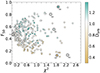 |
Fig. A.1. Orbit-to-orbit hardness variability relative to the hardness average trend. Each point represents an individual binary orbit from our sample (Sect. 4.1), with F50 (Eq. 3) values plotted against χ2 (Eq. A.1). Dorb coefficient (Eq. A.3) is colour-coded. We highlight the binary orbits shown in Fig. 7 with a black circle. See the main text for details. |
Appendix B: Light curve for an individual binary orbit
Figure B.1 shows an example of a MAXI/GSC light curve of an individual binary orbit for both soft and hard energy bands, illustrating unbinned and 1-day binned flux data distribution and variability across orbital phase bins.
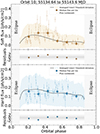 |
Fig. B.1. MAXI/GSC light curve for both the soft (top, yellow points) and hard (bottom, blue points) energy bands. Small squares represent unbinned flux data and large circles the median flux values per phase bin, each with their respective uncertainties. The bin size is indicated by the horizontal error bars. As in Fig. 3, the average trend is also shown as a solid black line and the standard deviation as a shaded area. |
All Tables
All Figures
|
Fig. 1. Vela X-1 as seen from Earth, with an orbital inclination (i > 73°) compatible with the known constraints (with parameters from Kreykenbohm et al. 2008). The black points represent the positions of the neutron star at specific phases (with origin at the mid-eclipse time). The red line is the main axis of the eccentric orbit. Owing to the eccentricity, inferior conjunction of the neutron star occurs between ϕorb = 0.4 and ϕorb = 0.5. The accretion wake trailing the neutron star is represented at a fiducial orbital phase ϕorb = 0.6. |
| In the text | |
|
Fig. 2. Four unfolded spectra of Vela X-1 from XMM-Newton observation (2019) taken with EPIC-pn. Each spectrum is ∼283 s and corresponds to a different absorption column density value, from low NH (light green) to high NH (dark blue). The observation covers the 0.37−0.51 orbital phase range (Diez et al. 2023). The shaded zones cover the MAXI/GSC energy bands chosen for our analysis (2−4 keV and 4−10 keV). |
| In the text | |
|
Fig. 3. Histograms and average trends of the MAXI/GSC dataset. Left: 2D histograms showing the unbinned MAXI/GSC dataset, depicting the flux in the 2−4 keV (soft band; top) and 4−10 keV energy range (hard band; middle), and the derived hardness ratio (bottom), calculated as explained in Sect. 3. The number of unbinned data points is colour-coded: lighter shades denote smaller values and darker shades indicate higher ones. Right: Average trends and their associated standard deviations derived from fits to the 2D histograms. Each shaded region is colour-coded, and the same code is used in Figs. 7 and B.1. For further details, we refer to the main text. |
| In the text | |
|
Fig. 4. Coefficient of variation (CV; see Eq. (2)) of the flux and hardness average trends from Fig. 3 (right panels). |
| In the text | |
|
Fig. 5. Histogram of hardness uncertainties derived from fluxes outside the eclipse region, as defined in Sect. 3.1. The threshold, indicated by a vertical line refines the sample by excluding hardness values with uncertainties exceeding 0.4. See further details in Sect. 4.1. |
| In the text | |
|
Fig. 6. Histogram of the F50 parameter (Eq. (3)) illustrating the streamlined classification as explained in Sect. 4.2.2, with vertical dashed blue lines indicating the defined thresholds for each type of hardness profile. We refer to the main text for further details. |
| In the text | |
|
Fig. 7. Orbit-to-orbit hardness profiles categorised into three groups based on F50 thresholds (Eq. (3)): harder (F50 > 0.6, top, blue), softer (F50 < 0.4, middle, red), and standard (0.4 ≥ F50 ≥ 0.6, bottom, green). Left column: Well-defined orbits. Right column: Orbits from the same group with larger variability (see Appendix A for a more elaborated statistical analysis derived from the analysis outlined in Sect. 4.2.2). We refer to the main text for further details. |
| In the text | |
|
Fig. 8. Absorption column density values across the orbital phase derived from multiple X-ray satellite observations adapted from Kretschmar et al. (2021). We refer to the main text for considerations when comparing absolute NH values. Different symbols are used to show data taken in different binary orbits by the same mission. The mean hardness profile from our MAXI/GSC sample is visually scaled and superimposed. The hardness ratio correlates positively with NH but lacks a direct one-to-one relationship, hence the need for an arbitrary scaling. |
| In the text | |
|
Fig. A.1. Orbit-to-orbit hardness variability relative to the hardness average trend. Each point represents an individual binary orbit from our sample (Sect. 4.1), with F50 (Eq. 3) values plotted against χ2 (Eq. A.1). Dorb coefficient (Eq. A.3) is colour-coded. We highlight the binary orbits shown in Fig. 7 with a black circle. See the main text for details. |
| In the text | |
|
Fig. B.1. MAXI/GSC light curve for both the soft (top, yellow points) and hard (bottom, blue points) energy bands. Small squares represent unbinned flux data and large circles the median flux values per phase bin, each with their respective uncertainties. The bin size is indicated by the horizontal error bars. As in Fig. 3, the average trend is also shown as a solid black line and the standard deviation as a shaded area. |
| In the text | |
Current usage metrics show cumulative count of Article Views (full-text article views including HTML views, PDF and ePub downloads, according to the available data) and Abstracts Views on Vision4Press platform.
Data correspond to usage on the plateform after 2015. The current usage metrics is available 48-96 hours after online publication and is updated daily on week days.
Initial download of the metrics may take a while.