| Issue |
A&A
Volume 674, June 2023
|
|
|---|---|---|
| Article Number | A147 | |
| Number of page(s) | 18 | |
| Section | Interstellar and circumstellar matter | |
| DOI | https://doi.org/10.1051/0004-6361/202245708 | |
| Published online | 16 June 2023 | |
Observing the onset of the accretion wake in Vela X-1
1
Institut für Astronomie und Astrophysik, Universität Tübingen,
Sand 1,
72076
Tübingen, Germany
e-mail: This email address is being protected from spambots. You need JavaScript enabled to view it.
2
European Space Agency (ESA), European Space Research and Technology Centre (ESTEC),
Keplerlaan 1,
2201 AZ
Noordwijk, The Netherlands
3
Quasar Science Resources S.L for European Space Agency (ESA), European Space Astronomy Centre (ESAC),
Camino Bajo del Castillo s/n,
28692
Villanueva de la Canada, Madrid, Spain
4
Université Grenoble Alpes, CNRS, IPAG,
38000
Grenoble, France
5
Instituto de Física de Cantabria (CSIC-Universidad de Cantabria),
39005,
Santander, Spain
6
IRAP, CNRS, Université de Toulouse, CNES,
9 Avenue du Colonel Roche,
31028
Toulouse, France
7
Lawrence Livermore National Laboratory,
7000 East Avenue,
Livermore, CA
94550, USA
8
European Space Agency (ESA), European Space Astronomy Centre (ESAC),
Camino Bajo del Castillo s/n,
28692
Villanueva de la Cañada, Madrid, Spain
Received:
16
December
2022
Accepted:
16
March
2023
Abstract
High-mass X-ray binaries (HMXBs) offer a unique opportunity to investigate accretion onto compact objects and the wind structure in massive stars. A key source for such studies is the bright neutron star HMXB Vela X-1 whose convenient physical and orbital parameters facilitate analyses and in particular enable studies of the wind structure in HMXBs. Here, we analyse simultaneous XMM-Newton and NuSTAR observations at ϕorb ≈ 0.36–0.52 and perform time-resolved spectral analysis down to the pulse period of the neutron star based on our previous NuSTAR-only results. For the first time, we are able to trace the onset of the wakes in a broad 0.5–78 keV range with a high-time resolution of ~283 s and compare our results with theoretical predictions. We observe a clear rise in the absorption column density of the stellar wind NH,1 starting at orbital phase ~0.44, corresponding to the wake structure entering our line of sight towards the neutron star, together with local extrema throughout the observation, which are possibly associated with clumps or other structures in the wind. Periods of high absorption reveal the presence of multiple fluorescent emission lines of highly ionised species, mainly in the soft-X-ray band between 0.5 and 4 keV, indicating photoionisation of the wind.
Key words: X-rays: binaries / stars: neutron / stars: winds, outflows
© The Authors 2023
 Open Access article, published by EDP Sciences, under the terms of the Creative Commons Attribution License (https://creativecommons.org/licenses/by/4.0), which permits unrestricted use, distribution, and reproduction in any medium, provided the original work is properly cited.
This article is published in open access under the Subscribe to Open model. This email address is being protected from spambots. You need JavaScript enabled to view it. to support open access publication.
1 Introduction
The prototypical eclipsing high-mass X-ray binary (HMXB) Vela X-1 is one of the brightest persistent point sources in the X-ray sky despite a moderate mean intrinsic luminosity of 5 × 1036 erg s−1 (Fürst et al. 2010). It lies at a relatively short distance of  kpc; see the review by Kretschmar et al. (2021) and references therein for this and other system parameters quoted in Sect. 1. The system consists of a B0.5 Ib supergiant, HD 77581 (Hiltner et al. 1972), orbited by an accreting neutron star with an orbital period of ~8.964 days (Kreykenbohm et al. 2008; Falanga et al. 2015). The mass and radius of HD 77581 have been estimated by different authors to be between ~20 and ~26 M⊙ and between ~27 and ~32 R⊙ (Table 4 in Kretschmar et al. 2021). A strong stellar wind with a mass-loss rate of ~10−6 M⊙ yr−1 (e.g. Watanabe et al. 2006; Falanga et al. 2015; Giménez-García et al. 2016) fuels the accretion of matter onto the neutron star and the pulsating X-ray emission with a fluctuating pulse period of ~283 s. The mass of the neutron star is estimated to be ~1.7−2.1 M⊙, which is on the heavier side of the typical mass distribution; see Table 4 in Kretschmar et al. (2021), and especially the estimates by Rawls et al. (2011) and Falanga et al. (2015).
As the orbital separation of the two components is only ~1.7R* (van Kerkwijk et al. 1995; Quaintrell et al. 2003), the neutron star is deeply embedded in the dense wind of the supergiant and significantly influences the wind flow. Due to the high inclination of the system of >73° (Joss & Rappaport 1984; van Kerkwijk et al. 1995, and others), observations at different orbital phases can sample different structures in the stellar wind as modified by the interaction with the neutron star. One notable feature is the varying absorption as a function of orbital phase, which was detected by many authors (see the overview Fig. 5 of Kretschmar et al. 2021). They found a typical decrease in the absorption after eclipse up to an orbital phase of 0.2–0.3 (Martínez-Núñez et al. 2014; Lewis et al. 1992) followed by a sometimes steep increase in the phase range of 0.4–0.6 (Haberl & White 1990), with a varying location in phase in individual observations and with generally high absorption at later orbital phases (Sato et al. 1986; Haberl & White 1990).
In addition to the variations in observed flux due to X-ray absorption, wind-accreting X-ray pulsars also usually show significant variability of the intrinsic X-ray flux caused by a complex interplay of factors, such as variations in the density of the accreted material and possible inhibition of accretion by interactions at the magnetosphere. (Martínez-Núñez et al. 2017). For individual observations, especially at softer X-ray energies, it is not always evident to distinguish absorption variations from those of the intrinsic emission. A study of variability in Vela X-1 by Fürst et al. (2010) based on INTEGRAL data in the hard X-ray band, which is only very slightly affected by absorption, found a log-normal distribution of the intrinsic flux values. On various occasions ‘low states’ or ‘off-states’ have been observed (see Table 1 in Kretschmar et al. 2021, with multiple references), but again not always with a clear distinction of intrinsic X-ray brightness versus high absorption.
Early on in the history of observations of this source, X-ray observations and optical-emission-line evidence suggested a wake structure trailing the X-ray source in the binary system (see references in Conti 1978). These structures can be caused by multiple processes. The neutron star moving highly supersonically through the dense stellar wind will lead to a bow shock with a trailing accretion wake. Photoionisation of the wind by the bright X-ray source can lead to the formation of a shock between the accelerating wind and the stalling photoionised plasma (Fransson & Fabian 1980), which can then lead to a trailing spiral structure, the photoionisation wake. X-ray heating and radiative cooling of the wind (Kallman & McCray 1982; Blondin et al. 1990) can create additional instabilities and filamentary structures, leading to stronger short-term variations. Tidal deformation of the mass donor can lead to enhanced wind flux in the direction of the neutron star, even if it does not fill its Roche Lobe. For close systems, this can develop into a dense ‘tidal stream’ (Blondin et al. 1991), which when deflected by coriolis force tends to pass behind the compact object, which explains the high absorption at later orbital phases. The density enhancement from such a tidal stream would be expected to be quite stable in orbital phase, while variations caused by an accretion wake would vary from orbit to orbit. According to Blondin (1994), in a specific system, there would be either a tidal stream between the star and the neutron star, or a photoionisation wake trailing the neutron star.
Vela X-1 has also been studied via X-ray line spectroscopy. Early studies (e.g. Becker et al. 1978; Ohashi et al. 1984) mainly focused on the pronounced iron-line complex visible also very clearly in eclipse. A broad FeKα emission line was also found by Sato et al. (1986), but these authors suspected further contributions to the overall line intensity from FeKβ as well as from fluorescent Κα lines of Si, S, Ar, Ca, and Ni. Further elements have been reported from spectra taken during or close to eclipse (Nagase et al. 1994; Sako et al. 1999; Schulz et al. 2002), including recombination lines and radiative recombination continua (RRC), as well as fluorescence lines. The variety of observed ionisation states is a strong indication of the presence of an inhomogeneous wind with optically thick, less ionised matter coexisting with warm photoionised plasma. Chandra/HETGS spectra from three orbital phases (0, 0.25 and 0.5) were analysed by Goldstein et al. (2004) and Watanabe et al. (2006), who found an eclipse-like spectrum around orbital phase 0.5, while the spectrum was dominated by the continuum around phase 0.25. Grinberg et al. (2017) revisited the observation at phase 0.25, analysing time intervals of low and high spectral hardness (i.e. different levels of absorption) separately and detected line features from high- and low-ionisation species of Si, Mg, and Ne, as well as strongly variable absorption. This again implied the presence of both cool and hot gas phases, possibly from the combination of an intrinsically clumpy stellar wind and a highly structured accretion flow close to the compact object. Analysing the grating spectrometer data of a long XMM-Newton observation at early orbital phases, Lomaeva et al. (2020) found emission lines corresponding to highly ionised O, Ne, Mg, and Si as well as RRC of O. In addition, these authors found potential absorption lines of Mg at a lower ionisation stage and features identified as iron L lines.
In our targeted observing programme with XMM-Newton and NuSTAR, we aimed to cover an interesting binary phase range in which we expect strong changes in absorption while the accretion and ionisation wakes are crossing the line of sight of the observer (Grinberg et al. 2017). In our previous work with NuSTAR (Diez et al. 2022), we observed strong absorption variability along the orbital phase. However, an in-depth study of the varying absorption cannot be explored with NuSTAR alone as we need coverage at lower energies, which is possible with XXMM-Newton. On the other hand, XXMM-Newton alone is not sufficient and we need NuSTAR to constrain the continuum, hence the necessity for simultaneous observation.
We introduce the datasets and their reduction in Sect. 2 followed by a presentation of the light curves extracted in different relevant energy bands in Sect. 3. Using the results, we proceed to the time-resolved spectral analysis in Sect. 4 and finally discuss our results in Sect. 5, focusing on the absorption variability. A summary is given in Sect. 6 and in Appendix A we describe the calibration issues we faced during this work between NuSTAR and XMM-Newton in detail.
2 Observation and data reduction
Vela X-1 was observed on 3–5 May 2019 as the science target of a simultaneous campaign with XMM-Newton and NuSTAR. We used the European Photon Imaging Camera pn-CCDs (EPIC-pn; Strüder et al. 2001), the EPIC Metal Oxide Semiconductor (EPIC-MOS; Turner et al. 2001), and the Reflection Grating Spectrometers (RGS; den Herder et al. 2001) on board XMM-Newton (Jansen et al. 2001) under Obs ID 0841890201. The NuSTAR data under Obs ID 30501003002 were analysed in Diez et al. (2022). In the present paper, we focus on the simultaneous analysis of the new EPIC-pn data with our previous NuSTAR work (updated with the current calibration files and software) in order to obtain a broadband mapping of the stellar wind along the orbital phase of the neutron star around the companion star. The simultaneous RGS data will be explored in a later work. Details about the observation are given in Table 1 and a sketch of the system during this observation is shown in Fig. 1. We note the much larger net XMM-Newton EPIC-pn exposure due to the low Earth orbit (LEO) of NuSTAR.
The orbital phases ϕorb are obtained with the ephemeris in Table 2 from Diez et al. (2022), which is derived from Kreykenbohm et al. (2008) and Bildsten et al. (1997) and where ϕorb = 0 is defined as T90. The time of phase zero is usually defined using T90 (the time when the mean longitude l is equal to 90°) or by Tecl (the mid-eclipse time). Explanations on how to convert T90 to Tecl can be found in Kreykenbohm et al. (2008). Table 1 also provides orbital phases with Tecl. In this work, we exclusively use T90 and all the mentioned times are corrected for the binary orbit.
We use HEASOFTv6.30.1, and to analyse the data, we use the Interactive Spectral Interpretation System (ISIS) v1.6.2-51 (Houck & Denicola 2000). ISIS provides access to XSPEC (Arnaud 1996) models that are referenced later in the text.
2.1 NuSTAR
We used the NuSTARDAS pipeline (nupipeline) v2.1.2 with the calibration database (CALDB) v20220608 applied with the clock correction. We proceeded to the extraction of the products as in Diez et al. (2022), using the updated pipeline and calibration files mentioned above. Briefly, we extracted a spectrum for every orbit of NuSTAR around the Earth and for every rotation of the neutron star with the previously derived pulse period of ~283 s. For the extraction of the source region, we used a smaller radius of ~60 arcsec to minimise the impact of the background. The uncertainties are given at 90% confidence and the events were barycentred using the barycorr tool from the NUSTARDAS pipeline. The spectra were rebinned within ISIS to a minimal signal-to-noise ratio (S/N) of 5, adding at least 2, 3, 5, 8, 16, 18, 48, 72, and 48 channels for energies in the ranges 3.0–10, 10–15, 15–20, 20–35, 35–45, 45–55, 55–65, 65–76, and 76–79 keV, respectively, as in our previous work.
Observations log.
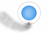 |
Fig. 1 Sketch of Vela X-1 showing the orbital phases covered during this XMM-Newton EPIC-pn observation. In this image, the observer is located facing the system at the bottom of the picture. |
2.2 XMM-Newton
The observation was setup in pn-timing mode with a thin filter. For the generation of the event lists file, we used the Science Analysis System (SAS) software v20.0 with the Current Calibration Files (CCF) as of April 2022 starting from Observation Data Files (ODFs) level running epproc1.
The default calibration uses withrdpha=‘Y’ and runepfast=‘N’ as of SASv14.02. However, this default timing mode calibration led us to an offset of the instrumental and physical lines of the source towards higher energies of ~+140eV (see Appendix A.1). Therefore, after consulting with the XMM-Newton calibration team (S. Migliari, priv. comm.), we decided to instead turn off the Rate-Dependent PHA (RDPHA) correction (withrdpha=‘N’) and apply the Rate-Dependent CTI (RDCTI) correction using epfast (runepfast=‘Y’), resulting in satisfactory spectra.
No filtering for flaring particle background was necessary. Because the source was so bright that it illuminated the whole CCD detector, no background was extracted. The event times were barycentred using the barycen tool from the SAS pipeline and were deleted if found to be on bad pixels with the #XMMEA_EP argument in the evselect step.
As XMM-Newton EPIC-pn and NuSTAR observations were simultaneous, we were able to reuse the pulse period previously derived on the FPMA light curve, P = 283.4447 ± 0.0004 s (Diez et al. 2022), to extract the XMM-Newton light curves in order to avoid intrinsic pulse variability. For a sanity check, we still performed epoch folding on the XMM-Newton light curve with 1 s binning and indeed derived the exact same pulse period as in our previous work.
We selected single and double pixel events (PATTERN<=4 in the evselect step) in the source region from RAWX=32 to RAWX=44. We removed the outermost parts of the point spread function (PSF) wings to reduce the influence of background noise or possible dust scattering effects. The count rate of the overall observation on different energy bands was sufficiently high to select a region of only 13 pixels centred around the maximum of the PSF. We applied the task epiclccorr to perform absolute and relative corrections.
2.3 Spectrum extraction and pile-up
For the extraction of the spectra, we performed the same selection of events as above, but we also deleted events close to CCDs gaps or bad pixels (FLAG==0 in the evselect step). An update to the EPIC effective area was made available in April 2022 to improve the cross-calibration between XMM-Newton and NuSTAR as of April 5, 20223. As we want to compare our XMM-Newton results to our previous NuSTAR ones, we activated this correction using the applyabsfluxcorr=yes argument in the arfgen step. All spectra were rebinned using the optimal rebinning approach of Kaastra & Bleeker (2016).
Because of the high count rate (see Sect. 3), the data were strongly affected by pile-up (Jethwa et al. 2015), in particular at the centre of the PSF. To test and evaluate for pile-up in our observation, we used the epatplot task to read the pattern information statistics of the input EPIC-pn set as a function of PI channel. As an additional sanity check, we performed an energy test on the iron line region (for more details, see Appendix A.2). According to the results of these tests, we decided to exclude the three centremost columns of the PSF (RAWX 37-38-39). Moreover, we excluded spectral channels below 0.5 keV and above 10 keV from the analysis where the S/N was very low.
We use this work to also report some cross-calibration issues between NuSTAR and XMM-Newton EPIC-pn. Cross-calibration issues between XMM-Newton EPIC-pn and NuSTAR are a known phenomenon when combining datasets from both observatories3 (see e.g. Gokus 2017) and the XMM-Newton Science Operations Centre is working on this issue with an upcoming update of the SAS software (S. Migliari, priv. comm.). At the time of writing, no release is available, and so we describe the cross-instrumental issues in Appendix A.3 and how we coped with them for our analysis in Sect. 4.2.
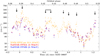 |
Fig. 2 Light curves for XMM-Newton EPIC-pn (orange), NuSTAR FPMA (red), and FPMB (blue) with a time resolution of P = 283.44 s. The count rate is plotted on the y-axis in logarithmic scale against the orbital phase (top axis) and the time of the observation (bottom axis). Major short flares are indicated by single arrows. The connected arrows at ~58607.42 MJD indicate a flaring episode of ~8 ks. |
3 Light curves and timing
3.1 Pulse period and average light curves
Strong flux variability was detected in Vela X-1 during this observation with timescales ranging from several kiloseconds down to the pulse period of the neutron star. To study the overall system behaviour, we present the 0.5–10 keV XMM-Newton EPIC-pn light curve in Fig. 2 together with the NuSTAR FPMA and FPMB 3–78 keV light curves.
The ratio of the XMM-Newton EPIC-pn count rate by the NuSTAR FPMA-FPMB count rate is not constant. During the first half of the observation (until Tobs ≈ 58607.60 MJD), the average XMM-Newton EPIC-pn count rate is ~30% higher than the NuSTAR one. Their ratio stabilises around 1 during the second half of the observation when the wakes are coming through our line of sight (see Fig. 1) and therefore when the absorption from the stellar wind is more prominent. As XMM-Newton EPIC-pn covers lower energies than NuSTAR, we expect it to be more affected by the absorption due to the stellar wind, explaining this behaviour.
All the major flares detected are indicated by arrows in Fig. 2. We can observe three flares happening simultaneously with both NuSTAR and XMM-Newton EPIC-pn at Tobs ≈ 58606.95 MJD, Tobs ≈ 58607.04 MJD, and Tobs ≈ 58607.42 MJD, and a fourth flare visible at Tobs ≈ 58608.23 MJD covered by NuSTAR only, as expected in Diez et al. (2022). With the new addition of EPIC-pn data, we can retrieve the data between Tobs ≈ 58607.57 MJD and Tobs ≈ 58607.76 MJD, which were lost during the NuSTAR campaign, and also retrieve data during the eclipses of the NuSTAR instrument. Therefore, we can observe three new flares at Tobs ≈ 58607.72 MJD, Tobs ≈ 58607.80 MJD, and Tobs ≈ 58607.93 MJD, together with the flare at Tobs ≈ 58607.42 MJD, which is longer than what was seen with NuS-TAR. This flare lasts ~8 ks and reaches ~300 counts s−1 which is almost as long as but brighter than the flaring period in Martínez-Núñez et al. (2014). The timescales of the flares appear to be from less than a NuSTAR eclipse (~2.5 ks) up to ~8 ks. The brightest observed flare at Tobs ≈ 58607.04 MJD reaches ~465 counts s−1 with EPIC-pn.
3.2 Energy-resolved light curves
To estimate the influence of the stellar-wind absorption on the observed count-rate variations, we extract the light curves in the relevant energy bands. In Diez et al. (2022), we saw a change in the hardness ratio between the 3.0–5.0 keV and 20.0–30.0 keV energy bands, roughly separating the observation into three noticeable phases: stable hardness ratio from the beginning of the observation to Tobs ≈ 58607.57 MJD, followed by the loss of the NuSTAR data until Tobs ≈ 58607.76 MJD, and finally the rise of the hardness ratio until the end. Fig. 3 shows three different XMM-Newton EPIC-pn spectra taken during the above-mentioned phases of the observation. We can observe low-energy variability towards the end of the observation (last panel of the figure). As expected from the geometry of the system (see Fig. 1), when the wakes occupy most of the line of sight of the observer, the absorption from the wind is so strong that the emission lines of the material become visible (see e.g. Watanabe et al. 2006). From the last spectrum, we can even highlight four energy bands of interest. The first one, from 0.5 keV to 3.0 keV, covers all the low-energy emission lines. We choose the second energy band from 3.0 keV to 6.0 keV to account for the low-energy part of the continuum before the iron-line region from 6.0 keV to 8.0 keV. The last energy band covers the high-energy part of the continuum from 8.0 keV to 10.0 keV. This will help us to compare the photon count rate in different energy bands relative to the continuum to check for variability. We present a more detailed spectral analysis in Sect. 4.
We present the XMM-Newton EPIC-pn light curves in the above-mentioned energy bands in Fig. 4. All light curves show the same features and variability in all energy bands, but the flares and low states are more prominent at low energies, particularly in the 0.5−3.0 keV energy band where the brightest flare is approximately five times higher than the average count rate in that band (~24 counts s−1). We notice a corresponding trend for the low state at Tobs ≈ 58 607.24 MJD, which is roughly five times smaller than the average count rate in the 0.5−3.0 keV band. The long and broad flare is visible in all energy bands but, again, is much more prominent in the 0.5−3.0 keV energy band and shows a rather stable plateau at ~40 counts s−1. In the two highest energy bands, the overall count rate stays relatively stable around the mean value of each individual light curve. This phenomenon was observed in a similar energy band, 1.0–3.0 keV, in Martínez-Núñez et al. (2014) and was associated with a stable spectral shape from the unabsorbed source.
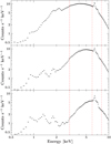 |
Fig. 3 XMM-Newton EPIC-pn spectra extracted during the three different phases of the observation. These are shown in chronological order from the top to the bottom panel: Phase of stable hardness ratio (0.37 ≲ ϕοrb ≲ 0.44), phase of the loss of NuSTAR data (0.44 ≲ ϕοrb ≲ 0.46), and phase of the rise of the hardness ratio (0.46 ≲ ϕorb ≲ 0.51), respectively. The vertical red dashed lines indicate the four energy bands we chose for the extraction of the energy-resolved light curves. |
3.3 Hardness ratios
For a more quantitative study of the source variability and in particular in an attempt to determine the origin of the variability shown in Vela X-1, we present the XMM-Newton EPIC-pn hardness ratios in Fig. 5. In the second panel, we observe a mirrored version of the light curve for the hardness ratio between the S = 0.5−3.0 keV and H = 8.0−10.0 keV bands. The minima of the hardness ratio correspond to the maxima of the light curve and vice versa. This shows that the observed flares of the light curve happen during the softening of the spectral shape, suggesting a contribution mainly from low-energy photons, as seen in Fig. 4. On the contrary, low states correspond to a hardening of the spectral shape, suggesting the major contribution is from high-energy photons. In the third panel, the hardness ratio between the S = 3.0–6.0 keV and H = 8.0–10.0 keV bands remains relatively constant until Tobs ≈ 58 607.60 MJD (ϕorb ≈ 0.44), with a local maximum at Tobs ≈ 58 607.24 MJD (ϕorb ≈ 0.40). The overall hardness ratio starts to increase after Tobs ≈ 58 607.60 MJD (ϕorb ≈ 0.44) until Tobs ≈ 58 607.93 MJD (ϕorb ≈ 0.48) followed by a steeper increasing slope until the end of the observation. This was expected from Diez et al. (2022) as we analysed similar energy bands for the hardness ratio: the 3.0–5.0 keV and 20.0–30.0 keV bands which also correspond to the low-energy and continuum parts of the spectrum, respectively. Finally, in the last panel of Fig. 5, the hardness ratio between the 6.0–8.0 keV and 8.0–10.0 keV bands is constant throughout the whole observation, showing no variation in the continuum as in Diez et al. (2022) and Martínez-Núñez et al. (2014).
In summary, it seems that the spectral shape gradually changes at low energies, which is particularly evident between 0.5 keV and 3.0 keV. This could be associated to changes in the behaviour of the absorbing material while the continuum emission from the neutron star seems to be stable.
Further insights into the role played by wind absorption come from a colour-colour diagram (Fig. 6) that shows a typical ‘nose’-like shape that has previously been associated with variable absorption in stellar wind, especially in Cyg X-1 (Nowak et al. 2011; Hirsch et al. 2019; Grinberg et al. 2020; Lai et al. 2022). We further discuss our modelling of the colour-colour diagram and its implications for the wind properties in Sect. 5.1.1. To further explore the behaviour of the source, a spectral analysis of the absorption column density on shorter timescales is necessary.
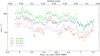 |
Fig. 4 Light curves for XMM-Newton EPIC-pn in different energy bands with a time resolution of P = 283.44 s. The count rate shown on the y-axis in logarithmic scale is plotted against the orbital phase and the time of the observation. The energy bands are 0.5−3.0, 3.0–6.0, 6.0–8.0, 8.0–10.0 keV. |
4 Spectral analysis
4.1 Definition of the spectral model
4.1.1 Continuum shape
As this current XMM-Newton EPIC-pn work follows results from simultaneous observations analysed in our previous NuSTAR work, we decided to use the same continuum model for direct comparisons and homogeneous continuity of the work. The final continuum model we obtained is the following and we refer to Diez et al. (2022) for a detailed discussion on how this model was obtained:
 (1)
(1)
The parameter NH,2 accounts for the absorption column density from the interstellar medium and is fixed to 3.71 × 1021 cm−2 using the NASA HEASARC NH tool website4 (HI4PI Collaboration 2016). The absorption NH,1 corresponds to the stellar wind embedding the neutron star and is a free parameter. Those two absorption components are described by the tbabs model (Wilms et al. 2000) with the corresponding abundances and cross-sections from Verner et al. (1996).
The covering fraction (CF) quantifies the clumpy structure of the stellar wind and ranges between 0 (the obscurer does not cover the source) and 1 (the obscurer is fully covering the source). This is characteristic of a partial covering model, of which several flavours can be found in the literature (e.g. Martínez-Núñez et al. 2014; Fürst et al. 2014a; Malacaria et al. 2016), and was found to provide the best description of the clumpy absorber in Vela X-1.
The function F(E) describes the spectral continuum of the accreting neutron star and is empirically described by a power law with a high-energy cutoff (see e.g. Staubert et al. 2019). Several models from the literature may account for the description of the high-energy cutoff. Our best results were obtained with the FDcut high-energy cutoff, whereby
 (2)
(2)
where Γ, Ecut, and Efold stand for the photon index, the cutoff energy, and the folding energy, respectively.
In the spectrum of Vela X-1, two cyclotron resonant scattering features (CRSFs, or cyclotron lines) are present with a prominent harmonic line at ~55 keV and a weaker fundamental at ~25 keV (Kendziorra et al. 1992; Kretschmar et al. 1997; Orlandini et al. 1998; Kreykenbohm et al. 1999, 2002; Fürst et al. 2014b; Diez et al. 2022). These features are typical of highly magnetised neutron stars and can be observed in the source X-ray spectrum as broad absorption lines. CRSFs result from resonant scattering of photons by electrons in strong magnetic fields from the ground level to higher excited Landau levels followed by radiative decay (see Staubert et al. 2019, for a review). We describe the CRSFs using two multiplicative Gaussian absorption lines with the gabs parameter in XSPEC, corresponding to the fundamental and harmonic CRSF, meaning that:
![Mathematical equation: ${\rm{CRSF}}\left( {\rm{E}} \right) = \exp \,\left[ { - \left( {{{\rm{d}} \over {\sigma \sqrt {2\pi } }}} \right)\,\exp \,\left( { - 0.5\,{{\left( {{{E - {E_{{\rm{cyc}}}}} \over \sigma }} \right)}^2}} \right)} \right],$](/articles/aa/full_html/2023/06/aa45708-22/aa45708-22-eq4.png) (3)
(3)
where d is the line depth and σ the line width.
The fluorescent emission line associated with FeKa is modelled with a narrow Gaussian line component with the egauss parameter in XSPEC around 6.4 keV, with width and flux left to vary. The 10 keV feature is described by a broad Gaussian line component in absorption. The physical origin of this feature is still unknown, but in Diez et al. (2022) we discussed the presence of this feature in Vela X-1.
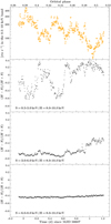 |
Fig. 5 Light curve and hardness ratios for XMM-Newton EPIC-pn. The first panel shows the overall count rate in the 0.5–10 keV energy band as in Fig. 2. The following panels show the hardness ratios between the mentioned energy bands. The time resolution is Ρ = 283.44 s. |
4.1.2 Line emission
Thanks to the low-energy coverage permitted by XMM-Newton EPIC-pn and a better resolution than NuSTAR between 3 and 10 keV, we now have access to new features that we need to include in our model. In our previous analysis, the fluorescent emission line associated with the FeKβ could not be resolved from the FeKα emission line. This is now possible with the XMM-Newton EPIC-pn energy resolution and we model it with a Gaussian component around 7.1 keV, with flux left free to vary but with fixed width.
Particularly in the most absorbed spectra of our observation, we can now also identify multiple emission lines between 0.5 keV and 4 keV (see last panel of Fig. 3). The absorption from the stellar wind is very strong towards the end of the observation (i.e. towards late orbital phases; see Diez et al. 2022), and therefore the strong continuum emitted by the neutron star is heavily absorbed and reveals the emission lines normally subsumed in the continuum when the absorption is less strong.
To help us to identify the energy of individual observed features, we based our search on Chandra/HETGS results of Amato et al. (2021), who analysed Vela X-1 at orbital phase ϕorb ≈ 0.75, which is even more affected by the stellar wind (see Fig. 1). Because of the limited energy resolution of EPIC-pn, Doppler shifts with orbital phase and triplets or faint lines cannot be resolved in this work. To search for the lines in EPIC-pn spectra, we had to fix the features (such as the CRSFs and the 10 keV feature) and continuum parameters (such as Ecut and Efold) that are not covered by the EPIC-pn instrument. We fixed them to the average NuSTAR values from Diez et al. (2022) for highly absorbed spectra to have an accurate description of the continuum in order to focus on the line description. We performed this search ‘by hand’, fitting Gaussian components to observed line features in the most absorbed time-resolved spectra of the observation until we obtained a satisfactory reduced chi-square. An example of such a spectrum is shown in Fig. 7. The energies of the narrowest lines (Ne X Lyα, Mg XII Si XIV Lyα, S XVI Lyα, Ca II−XIII Κα) have to be fixed to previous studies and their widths to 10−6 keV.
A list of the soft lines identified in this work and a comparison with previous studies is shown in Table 2. We note that, here we do not aim to perform an in-depth study of the emission-line variability but rather an absorption study of the stellar wind in Vela X-1. The instrumental issues described in Sect. 2 with the limited energy resolution of EPIC-pn can explain the discrepancies obtained for some lines in comparison with previous work, in particular for Ο VIII Lyα and Ca II–XII Κα. The Ar VI–IX and Ca II-XII Κα lines were not detected in Amato et al. (2021). However, those lines were identified in Schulz et al. (2002), Goldstein et al. (2004), and Watanabe et al. (2006) for Vela X-1 and in Fürst et al. (2011) for the HMXB GX 301–2. The different charge states of Ca and Ar cannot be resolved, and so in Table 2 we give the potential candidates as in Schulz et al. (2002) and Watanabe et al. (2006).
We also detect a 3.2 keV line that has not been reported in previous work. This feature can most likely be attributed to the S XV RRC, with its ionisation potential of 3.224 keV (Drake 1988). While lower charge states of Ar are present (2.9661 keV), the line energies for both He-like Ar XVII r at 3.140 keV (Drake 1988) and Η-like Ar XVIII Lyα at 3.321 keV (Garcia & Mack 1965) are too far away to reasonably match the fitted line energy. The same is true for the Η-like S XVI Lyβ and Lyγ lines at 3.106 and 3.276 keV (Garcia & Mack 1965), respectively, even though the S XVI Lyα feature is clearly detected. If this feature were indeed caused by the S XV RRC, we would expect RRC features from the more abundant ions as well. However, at the low resolution of the CCD spectra, many of the other RRC candidates are too blended to allow for a clear detection; for instance, the Si XIII RRC at 2.438 keV (Drake 1988) blends with the S XV Heα complex, the Ne X RRC at 1.362 keV (Garcia & Mack 1965) blends Mg XI Hea, and the Ο VIII RRC at 0.871 keV (Garcia & Mack 1965) with the Ne IX Heα lines (see e.g. Sako et al. 1999).
Finally, our final and best-fit model, which we use for the time-resolved spectroscopy in this work, is:
![Mathematical equation: $\matrix{ {I\left( E \right) = {N_{{\rm{H,2}}}} \times \left[ {\left( {{\rm{CF}} \times {N_{{\rm{H,1}}}} + \left( {1 - {\rm{CF}}} \right)} \right) \times \left( {F\left( E \right) \times {\rm{CRSF,}}\,{\rm{F}}} \right.} \right.} \hfill \cr {\left. {\,\,\,\,\,\,\,\,\,\,\,\,\,\,\,\,\,\,\,\left. { \times \,{\rm{CRSF,}}\,{\rm{H}}} \right) + {\rm{FeK}}\alpha \,{\rm{ + }}\,{\rm{FeK}}\beta + {\rm{10}}\,{\rm{keV}}\,{\rm{ + }}\,{\rm{Soft}}\,{\rm{lines}}} \right].} \hfill \cr } $](/articles/aa/full_html/2023/06/aa45708-22/aa45708-22-eq20.png) (4)
(4)
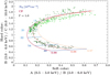 |
Fig. 6 XMM-Newton EPIC-pn colour-colour diagram. The data points represent the ratios of the light curves in hard colour depending on soft colour, from beginning (light green) to end (dark green) of the observation. We also show the theoretical expectation for different covering fractions CF (shades of red, varying from 0.97 to 0.99) and absorption column densities NH,1 (shades of blue, varying from 3 × 1022 cm−2 to 80 × 1022 cm−2) using our partial covering model from Eq. (4). We used a photon index Γ of 1.0. More details about the simulation and its interpretation are given in Sect. 5.1.1. |
Details of soft emission lines between 0.5 keV and 4 keV.
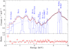 |
Fig. 7 Example XMM-Newton EPIC-pn spectrum (black datapoints). We show the last and most absorbed NuSTAR-orbit of our observation. We indicate the individual model components including all lines detected in this dataset (blue dot-dashed Gaussians) and the absorbed continuum (blue dotted line). We refer to Sect. 4.2 for a detailed description of the model and to Table 2 for the soft lines. |
4.2 NuSTAR-orbit-by-orbit analysis
We can now perform the analysis on shorter timescales with both XMM-Newton EPIC-pn and NuSTAR to access the variability of the stellar wind at low energies. Combining both datasets – and thus increasing the covered spectral range – limits the impact of possible degeneracy between the power-law slope and absorption strength. NuSTAR data are especially crucial at high absorption, when it is especially difficult to constrain the continuum with XMM-Newton only.
In Diez et al. (2022), we extracted a spectrum for every orbit of NuSTAR around the Earth, which is referred to here as ‘NuSTAR-orbit’ for the remainder of the paper. This should not be confused with the duration of a binary orbit of the neutron star around its companion. For the simultaneous XMM-Newton EPIC-pn data, we decided to extract a spectrum using the same good time intervals (GTIs) used for the NuSTAR-orbit-by-orbit analysis with NuSTAR data in order to have a broad X-ray band description of the stellar wind on the same timescale. Due to the different start and stop times of the observations, there are NuSTAR-orbits without simultaneous XMM-Newton EPIC-pn data (see Fig. 2). Moreover, during the NuSTAR campaign, data were lost because of ground-station issues, resulting in no or limited NuSTAR coverage for parts of our XMM-Newton observation. For the ‘missing’ NuSTAR-orbits, we took the average duration of a NuSTAR-orbit, which lasts -0.067 MJD (~5.8 ks), in order to extract XMM-Newton EPIC-pn spectra. Overall, we have 1 NuSTAR-orbit covered by NuSTAR only, 2 NuSTAR-orbits covered by XMM-Newton EPIC-pn only, 4 NuSTAR-orbits partially covered by one of the two instruments, and 14 NuSTAR-orbits fully covered by both instruments (Fig. 8). We fit the data using the model from Eq. (4), with adaptations as necessitated by the different instrumental coverage as discussed in the following.
Firstly, for the NuSTAR-orbits covered by both NuSTAR and XMM-Newton EPIC-pn, we use a floating cross-normalisation parameter, CNuSTAR, in order to give the relative normalisation between the two NuSTAR detectors FPMA and FPMB with the XMM-Newton EPIC-pn instrument. The difference between FPMA and FPMB is of the order of ~2%, and so we can safely assume one normalisation constant to account for both focal plane modules for simplicity.
As discussed in Sect. 2, cross-calibration issues between NuSTAR and XMM-Newton EPIC-pn are impacting the analysis. To correct the observed up-turn in the NuSTAR data at ~3 keV, we applied two different CFs, CFXMM and CFNuSTAR, for XMM-Newton EPIC-pn and NuSTAR, respectively. We do not fix CFNuSTAR to previous values from Diez et al. (2022) as this current work benefits from low-energy coverage with XMM-Newton, which gives us better constraints on NH,1, and therefore on CFNuSTAR, because those two parameters were found to be strongly correlated, as shown in Fig. 7 of Diez et al. (2022). To correct the shift in the FeKα emission line, we apply a gain shift to the NuSTAR data in order to align on the iron line energy found with XMM-Newton EPIC-pn.
We also introduce another cross-normalisation constant CFe to account for the flux difference observed in NuSTAR relative to XMM-Newton EPIC-pn in the emission lines that are covered by both observatories: FeKα and FeKβ. We fix the soft-emission-line energies and widths to the values estimated when analysing the XMM-Newton EPIC-pn spectrum at high absorption (see Table 2) as they are not expected to change significantly with time, even if the source is highly variable (Grinberg et al. 2017). The fluxes of the emission lines are left free as their prominence changes depending on the local absorption.
We fix the CRSF parameters and the energy of the 10 keV feature to the values of their corresponding NuSTAR-orbit – which we obtained in our previous analysis in Diez et al. (2022) - to help to constrain the low-energy part of the continuum. Degeneracies between ECRSF,F and Ecut are expected due to their proximity as seen in Diez et al. (2022); therefore, we also fix the cutoff energy in the same way.
Secondly, for the two NuSTAR-orbits only covered by XMM-Newton EPIC-pn (NuSTAR-orbits number 12 and 13), we fix the CRSFs parameters, the energy of the 10 keV feature E10 keV, and the cutoff energy Ecut to the closest NuSTAR-orbit values. These parameters cannot be ignored during the fitting because they modify the shape of the broadband continuum, and therefore fixing them to the values of the closest NuSTAR-orbit is the most accurate and meaningful solution. We do not use CNuSTAR, gain shift, CFNuSTAR, or CFe as there is no need to correct for cross-calibration because no coverage from NuSTAR is available for those NuSTAR-orbits.
Thirdly, for the NuSTAR-orbit that is covered by NuSTAR only (NuSTAR-orbit number 1), the multiple soft emission lines and the FeKβ line identified with XMM-Newton EPIC-pn are not resolved by NuSTAR alone. However, those emission lines do not impact the shape of the overall continuum of Vela X-1, and therefore they can be safely ignored for fitting the data for simplicity. We tried to fix them to the values of the closest following NuSTAR-orbit but no significant difference could be highlighted when comparing the residuals.
We present the results of the NuSTAR-orbit-by-orbit analysis in Fig. 8, focusing on the parameters of interest. An example of a fitted spectrum extracted during one NuSTAR-orbit with both XMM-Newton EPIC-pn and NuSTAR is given in Fig. A.4. However, we caution that the different instrumental coverage of individual spectra may result in artificial parameter behaviour, such as outliers.
Discrepancies between NuSTAR and XMM-Newton EPIC-pn are visible in the cross-normalisation parameter CNuSTAR, reaching ~20% (not considering outliers), which can be explained by the low-energy up-turn in NuSTAR (see Fig. A.4). Moreover, the average energy gainshift of NuSTAR relative to XMM-Newton EPIC-pn is of −87 eV. This particularly impacts the iron line region as it is covered by both instruments. Therefore, the energy of the iron line shown in the third panel of Fig. 8 is given with respect to the XMM-Newton EPIC-pn values, and the gainshift has to be added to retrieve the NuSTAR values, with the exception of the magenta triangle outlier of NuSTAR-orbit 1, which is only covered by NuSTAR.
Significant variability can be observed in the presented parameters. In particular, NH,1 increases by a factor of 6 between the beginning and the end of the observation, showing a very clear rise of the stellar-wind absorption at ϕorb ≈ 0.44–0.49. The energy of the iron line remains relatively stable around ~6.48 keV, but shows local minima, which seem to be anti-correlated with the flux in the 3–10 keV energy band. This anti-correlation with flux appears to be similar for the photon index, which also shows local dips during flares. The photon index varies overall between 0.8 and 1.2, the change of spectral shape being associated with changes in absorption density in the stellar wind and possible degeneracy with the amount of absorption. We discuss the details of these relationships and a further investigation of them in Sect. 5.
While the CF with XMM-Newton EPIC-pn CFXMN remains very stable around 0.98, the CF with NuSTAR is much more variable, ranging between 0.3 and 0.98 (we note the different y-axis range compared to CFXMN) as in Diez et al. (2022) when analysing NuSTAR data alone. This is due to the up-turn in NuSTAR data at low energies (see Fig. A.4). We discuss tests performed to assess some possible sources of this effect in Appendix A.3, and in particular a possible contribution from dust scattering. We are unable to find a plausible physical explanation and therefore conclude that the problem is due to some remaining calibration effects. In Diez et al. (2022), we discussed the problems encountered with the low-energy effective area correction for FPMA (Madsen et al. 2020) in our observation. While these problems should not affect FPMB, together with the high variability of the CF as deducted from the NuSTAR data alone, they imply a reduced reliability of the NuSTAR data for our observation in this energy range. Moreover, looking at Fig. 6, it is obvious that a CF of less than 0.97 would not describe the data. We therefore decide to focus our discussion on XMM-Newton-driven CF values for the remainder of the paper.
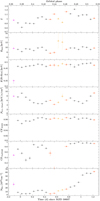 |
Fig. 8 Results of the NuSTAR-orbit-by-orbit analysis with NuSTAR and XMM-Newton as a function of time, together with the corresponding binary orbital phase. From top to bottom: Photon index (Γ), folding energy (Efold) in keV, energy of the FeKα line in keV, unab-sorbed flux ℱ0.5−78,keV in keV s−1 cm−2, CFs with NuSTAR (CFNuSTAR) and XMM-Newton EPIC-pn (CFXMN), absorption from the stellar wind NH,1 in 1022 cm−2. Circles show data fully covered by both XMM-Newton EPIC-pn and NuSTAR. Triangles show data missing coverage from one of the two instruments. Magenta marks the data only covered by NuSTAR (NuSTAR-orbit 1) and orange the data fully covered by one instrument but partially by the second one (NuSTAR-orbits 10, 11, 14 and 21). Finally, yellow is used to denote data only covered by XMM-Newton EPIC-pn (NuSTAR-orbits 12 and 13). |
4.3 Pulse-by-pulse: XMM-Newton only
The sensitivity of XMM-Newton EPIC-pn allows us to extract a spectrum down to the pulse period of the neutron star (283 s). We performed a spectral analysis for every pulse of the neutron star to explore further variability on shorter timescales.
Given the cross-instrumental issues between XMM-Newton and NuSTAR and the different coverage of the overall observation (due to both LEO of NuSTAR and the loss of data), this analysis is performed on XMM-Newton data only. While for the NuSTAR-orbit-by-orbit analysis it was still possible to safely determine the individual contribution of each instrument for each GTI and exclude outliers when needed, such an approach is not feasible for the pulse-by-pulse analysis. The pulse-by-pulse results for this observation with NuSTAR only are presented in Diez et al. (2022).
We again use the model from Eq. (4), setting up the initial parameters for each pulse spectrum from the results of the corresponding NuSTAR-orbit of the NuSTAR-orbit-by-orbit spectral analysis. Given the low signal of the individual datasets, we fix all parameters but the photon index Γ, the covering fraction CFXMN, the absorption column density from the stellar wind NH,1, the energy of the fluorescent FeKα line, and the flux of all the emission lines.
In Fig. 9, we present the results of the pulse-by-pulse analysis for the XMM-Newton EPIC-pn data. The typical reduced chi-square  of the fittings is ~1.20 and the time resolution of ~283 s gives us access to much more parameter variability along the orbital phase than in Fig. 8. Again, the rise of the absorption column density NH,1 is clearly visible but with much more local instability, such as two local episodes of high absorption at orbital phases ~0.40 and ~0.44. The overall track is very similar to the hardness ratio between the 3–6 keV and 8–10 keV energy bands shown in the third panel of Fig. 5 and is even more amplified on the second panel of the same figure for the hardness ratio between the softest and hardest energy bands. This is expected as mainly low-energy photons are absorbed by the stellar wind, and therefore the underlying spectral shape becomes harder during those high-absorption episodes, as explained in Sect. 3. On the other hand, episodes of low absorption seem to be associated with flaring periods according to Fig. 9, which could be explained by accretion of clumps on the line of sight of the observer, as described in Diez et al. (2022). In Diez et al. (2022), we observed a correlation between CFNuSTAR and NH,1, but also with flux. However, there does not seem to be any correlation between XMN-Newton-driven CF values and NH,1 or flux ℱ for this work. The photon index Γ is relatively variable, particularly towards the end of the observation. This should be taken with caution as the error bars get larger and the absorption is so strong that there may be some degeneracy between NH,1 and Γ.
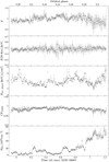 |
Fig. 9 Results of the pulse-by-pulse analysis as a function of time, together with the corresponding binary orbital phase. The panels show (from top to bottom) photon index (Γ), energy of the FeKα line in keV, unabsorbed flux ℱ0.5–10 keV in keV s−1 cm−2, CF with XMM-Newton EPIC-pn (CFXMN), and absorption from the stellar wind NH,1 in 1022 cm−2. |
5 Discussion: The variable absorber
5.1 Evolution of absorption along the binary orbital phase: the onset of wakes
The main finding of our paper is the detailed analysis of the rise of the NH,1 value and therefore of the absorption in the stellar wind, which we interpret as the onset of the wakes. This is the first time this orbital period and the corresponding wind structure are probed in a time-resolved way with a modern X-ray instrument (see Fig. 5 in Kretschmar et al. 2021).
5.1.1 X-ray colour evolution with orbital phase
We observe an interesting gradual increase in the hardness ratio between the 3.0–6.0 keV and 8.0–10.0 keV energy bands (see third panel of Fig. 5). This is more a consequence of a general geometric change in the stellar wind than of the local accretion of clumps. When the wakes are coming through our line of sight (see Fig. 1), the absorption in the stellar wind increases, preferentially absorbing low-energy photons emitted in the vicinity of the neutron star starting from ϕorb ≈ 0.44. In our pulse-by-pulse analysis, this rise in the absorption column density NH,1 can be directly measured from Fig. 9.
On the other hand, the hardness ratio of high-energy bands is constant (last panel of Fig. 5), implying a stable behaviour of the continuum emission from the neutron star. Martínez-Núñez et al. (2014) observed similar behaviour - spectral changes at low energies due to increasing absorption but stable overall source continuum – during their observation, which covered eclipse egress and a major flare.
The above is supported by the behaviour of the source on the colour-colour diagram (Sect. 3.3) where it describes a nose shape (Fig. 6). This is typical of the presence of a partial coverer with variable column density in the system (e.g. Hirsch et al. 2019; Grinberg et al. 2020, in Cyg X-1). As would be expected given the onset of the wake, the source evolves along the track with time, as indicated by transition from light (early in the observation) to dark green (late in the observation) data points in the figure.
Figure 10 shows how absorption impacts the observed spectrum modelled by Eq. (4), which consists of a power-law continuum with a high-energy cutoff, assuming a certain CF. In the case of a continuum fully covered by the obscurer (CF = 1, dashed lines), the flux ratios in the soft colour (A/B) and in the hard colour (B/C) decrease as NH,1 grows, leading to a positive correlation between those ratios for the covered spectrum. On the other hand, if we consider a spectrum where this time only a certain fraction CF < 1 of the continuum is absorbed by the stellar wind (solid lines), the flux in the A band will remain constant as NH,1 grows after a certain threshold. In the example of a covering fraction of 0.9, this happens at NH,1 = 54 × 1022 cm−2 according to expectations from Fig. 10. Simultaneously, the fluxes in the B and C bands continue to decrease together as NH,1 grows. Hence, the softer colour becomes softer as the harder colour does not change, leading to the observed nose-shape colour-colour diagram in Fig. 6. This probes the necessity of a partial covering model to describe the data. A higher CF leads to a less elongated curve.
We use an averaged Γ over the values obtained in Fig. 8 for our observation. We simulate a grid of colour-colour tracks for varying values of NH,1 and covering fraction and include the results in Fig. 6. Data and simulations agree very well, supporting our interpretation.
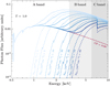 |
Fig. 10 Effect of increasing absorption on our model from Eq. (4) with photon index Γ = 1.0 and without emission lines to focus on the evolution of the continuum shape. We assume a CF of 0.9 and a varying absorption column density NH,1 from 3 × 1022 cm−2 to 80 × 1022 cm−2 covering the range obtained in Fig. 9. The shaded grey areas indicate three energy bands of interest: The A band from 0.5 to 3 keV, B band from 3 to 6 keV, and C band from 6 to 10 keV. The resulting observed spectrum (solid lines) is the sum of the spectrum not covered by the stellar wind (dash-dotted line) and the covered spectrum (dashed lines). See Fig. 3 of Diez et al. (2022) for an illustrated picture of the partial covering model. |
5.1.2 Comparison with previous observations and model descriptions
While absorption values have been determined by many authors with various different satellites (see Kretschmar et al. 2021, for an overview), there are few data sets that cover a significant range in orbital phase within an individual binary orbit and therefore that do not mix potential binary orbit-to-orbit variations in wake structures. After correcting for differences in orbital phase definitions in the original papers, in Fig. 11 we compare the absorption values we derived with data points from Ohashi et al. (1984) and Haberl & White (1990). Different spectral models used to fit spectra and to derive NH may introduce systematic shifts in the obtained values. Still, the data taken over many years appear to cover a similar range, but sometimes with quite different values at the same orbital phase, as seen already in Kretschmar et al. (2021), indicating that the structures causing these variations are not stable in orbital phase. On the other hand, the duration of the overall rising trend from low absorption to a highly absorbed ‘plateau’ is rather similar in slope – NH values double over a time range of 0.02 in orbital phase or ~15.4 ks – suggesting that similar larger structures in the wind exist, which may differ somewhat in their relative orientation.
In Fig. 12, we compare our derived NH values with some of the few examples of column densities derived from hydro-dynamical model calculations. However, it is important to note that these models start from quite different assumptions (see also Table 3) and were not made for direct comparison. First of all, the curves shown for the models of Manousakis & Walter (2015b) and Manousakis et al. (2012) are time-averaged values of column density over orbital phase, smoothing out the expected significant NH variability from binary orbit to binary orbit, while the result from Blondin et al. (1991) is taken from the simulation of a single binary orbit in a model including a tidal stream. It is evident that neither this last model nor the relatively low and little varying average column density predicted by Manousakis & Walter (2015b) shows a marked rise at early orbital phases as found in the data. One of the reasons for this may be the rather high wind velocities and mass-loss rates assumed in these studies, and certainly found in earlier studies of Vela X-1, while more modern studies assume lower wind velocities (see Table 7 and Fig. 19 in Kretschmar et al. 2021). The visually best matching curve from Manousakis et al. (2012) was, on the other hand, calculated for a different system, EXO 1722−363, albeit with relatively similar system parameters to Vela X-1, and assuming a relatively slow wind. Updated hydrodynamical simulations accounting for the current best knowledge of orbital and wind parameters of the system, and taking the non-negligible eccentricity into account, would be very welcome.
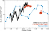 |
Fig. 11 Comparison of the NH values determined in this study with historical measurements taken during individual binary orbits by Tenma (Ohashi et al. 1984) and EXOSAT (Haberl & White 1990). We highlight the overall similar slope of the different rising curves. See text for details. |
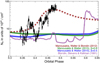 |
Fig. 12 Comparison of the NH values determined in this study with a range of model results for NH from hydrodynamic simulations for Vela X-1 or similar, but not identical model systems. See the main text and Table 3. |
5.2 Origin and nature of the absorber
The continuum from the neutron star dominates the emission in the spectrum of Vela X-1 until ϕorb ≈ 0.44. At this orbital phase, the absorption column density increases together with the strength of soft emission lines between 0.5 and 4 keV. Figure 13 shows the evolution of the flux of some lines with time. In particular, we can see the fluxes of the Ne IX and S XV are mostly consistent with 0 at the beginning of the observation but start to increase towards the end, revealing the corresponding elements in the spectrum of Vela X-1. The presence of strong lines during heavy absorption from the stellar wind suggests that the absorber is localised and the lines originate from a larger scale in the system, as in Watanabe et al. (2006). If these lines originated from the local absorber or close to the vicinity of the neutron star, they would be completely absorbed by the stellar wind and would not appear in the resultant spectrum. Another argument in the favour of this statement is that those soft emission lines are also present in the spectrum of Vela X-1 during the eclipse (Sako et al. 1999), which is when the neutron star and its local absorber are outside the line of sight of the observer.
In Fig. 13, the fluxes of the fluorescent FeKα and FeKβ lines are positive throughout the whole observation, meaning that those lines are visible at all observed orbital phases here and therefore also originate from a larger scale in the system. The situation is less evident for the fluorescent Ca II-XII Kα line, which was more difficult to constrain because of blending with neighbouring lines.
The Ne IX, Mg XI, Si XIII, and S XV complexes are evidence of ionisation of the absorber in the system, as those ions only have two remaining electrons on their orbital. Furthermore, the presence of O VIII, Ne X, Mg XII, Si xiv, and S XVI Lyα lines also indicates ionisation in the system as they are emitted when the last atomic electron transitions from an n = 2 orbital to the ground state. According to Amato et al. (2021), the warm pho-toionised wind of the companion star and smaller cooler regions or clumps of gas can explain the simultaneous contribution of H- and He-like emission lines and fluorescent lines of near-neutral ions. Comparing Chandra/HETGS data of Vela X-1 with simulations of propagation of X-ray photons in a smooth and undisturbed wind, Watanabe et al. (2006) stated that fluorescent lines originate from reflection of the stellar photosphere in the extended stellar wind or simply from the accretion wake. Additionally, these authors observed brighter soft emission lines at ϕorb = 0.5 than during the eclipse. This indicates a higher production of X-ray line emission caused by highly ionised ions in a region between the neutron star and its massive stellar companion, which is occulted during eclipse. However, this is difficult to confirm with our data and further studies at higher spectral resolution are necessary.
5.3 Short-term absorption variability
5.3.1 Search for characteristic timescales in absorption variability
Theoretical predictions show that variability in a clumpy material can result in typical variability timescales that will depend on the properties of the structures in the stellar wind and/or in the tidal streams in correlation with the orbital parameters of the system (El Mellah et al. 2020). In this section, we therefore present a search for possible indications of such a timescale. To perform this analysis, we used the Stingray: A Modern Python Library for Spectral Timing (Bachetti et al. 2022; Huppenkothen et al. 2019a,b) Python library. Our pseudo-light curve of NH contains 392 bins with a binning size equal to the pulse period of the neutron star (~283 s). We used different techniques implemented in Stingray, which are:
average power spectrum using Leahy normalisation and dividing our data into 11 subsets. This technique allows the search for periodicities in the frequency range between 0.0002 and 0.00175 Hz (see panel a of Fig. 14);
z-search and chi-search techniques to search for periodicity in the frequency range between 0.006 and 0.0033 (see panels b and c of Fig. 14 respectively).
Neither of the techniques detects a significant periodic or quasi-periodic signal in the evolution of NH in the range of frequencies accessible with our data. The simulations of El Mellah et al. (2020) predict a clear signal in the autocorrelation function equivalent to a cutoff in the power spectrum. Given the quality of our data, the presence of such a feature cannot be assessed. Still, the spectrum presented above is, to our knowledge, the first absorption power spectrum calculated for Vela X-1 in an attempt to obtain such timescales.
To expand the frequency search range to larger values, we also performed a Lomb-Scargle periodogram using the routine of Astropy v5.1 Timeseries software (Astropy Collaboration 2022) (see panel d of Fig. 14). This technique only finds the binning size of our database (and following harmonics) as a possible period but no other periodicity could be found. It does not allow the shape of the power spectrum to be assessed. This search could be enhanced with an extended sample of the NH along one or more binary orbits.
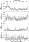 |
Fig. 13 Fluxes in photons s−1 cm−2 of some soft lines obtained within the pulse-by-pulse analysis as functions of time, together with the corresponding binary orbital phase. The panels show (from top to bottom) the flux of the FeKα, the FeKβ, the Ne IX, and the S XV line. |
5.3.2 Absorption during flares
During the first two flaring episodes at ϕorb ≈ 0.38 and ϕorb ≈ 0.43, we saw in the second panel of Fig. 5 that the hardness ratio between the continuum band and the softest band decreases dramatically, indicating a softening of the underlying spectrum. This is also confirmed in Fig. 8 with the local decreases in photon index during flaring episodes. Therefore, more low-energy photons are detected compared to before the flaring episodes. If more low-energy photons reach the detector plane, this suggests that there is less material on the line of sight of the observer (otherwise they would have been absorbed by the wind), and therefore less absorption from the stellar wind. This is confirmed by our time-resolved spectral analysis in Fig. 8 and in Fig. 9, where the absorption column density of the stellar wind NH,1 reaches its minimum during those two flaring episodes.
This is also visible during later short flares with strong but brief softening of the spectral shape together with local minima of NH,1 and CF. These short-timescale events could be associated with the accretion of clumps in the vicinity of the neutron star, as already suggested in Martínez-Núñez et al. (2014) and Diez et al. (2022) for Vela X-1. As material falls onto the surface of the neutron star through the accretion column, photons are produced through bremsstrahlung and cyclotron emission. Those photons are then up-scattered through inverse Compton and more X-rays are produced. The more material falls into the neutron star, the more the temperature increases, favouring interactions and X-ray production. Clumps just passing in front of the source on the line of sight of the observer could explain the local maxima in NH,1 that are not happening simultaneously with flux changes.
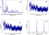 |
Fig. 14 Timing analysis of NH evolution: (a) Stingray average power spectrum; (b) Stingray z-square function; (c) Stingray chi-square function; (d) Astropy v5.1 Lomb-Scargle Periodogram. |
6 Summary and outlook
We analysed simultaneous XMM-Newton and NuSTAR data of Vela X-1 covering a broad X-ray range at orbital phase ~0.36–0.52. For the spectral modelling, we used our partial covering model first described in Diez et al. (2022). Thanks to the hard X-ray coverage permitted by NuSTAR and our results from previous work, we were able to constrain the continuum in order to focus on the absorption variability at lower energies with XMM-Newton EPIC-pn for this work.
This is the first time that such a high-time-resolution absorption study of Vela X-1 has been carried out on a broad X-ray range from 0.5 to 78 keV. We traced the onset of the wakes, which are characterised by a rise in the absorption column density NH,1 starting at orbital phase ~0.44 as well as local absorption variability due to the accretion of clumps. The slope of the NH,1 rise is comparable, and is similar to previous observations, albeit with an orbital-phase lag indicating similar large-scale structures in the wind but with different orientation at different times of observation. We also compared our data with simulations from previous works in the literature but no strong match between observations and theoretical models could be found. This reflects the necessity for further and updated hydrodynamical simulations that account for the latest orbital parameter values (for example: eccentricity >0) and the complexity of the wind parameters (such as wind velocities and mass-loss rates).
Through high-resolution spectroscopy of the multiple fluorescent lines present in Vela X-1, we performed X-ray photography of the material in the system. The evidence of those lines at different absorption phases suggests sources of emission from local absorber to large-scale structures. This analysis also reveals strong photoionisation of the wind with the presence of highly ionised elements such as Lya lines of O, Ne, Mg, Si, and S. However, these results have to be considered with caution as the XMM-Newton EPIC-pn energy resolution is not sufficient to perform an accurate spectral analysis of individual lines and blending with neighbouring elements can happen. This aspect is beyond the scope of this paper and the analysis of simultaneous XMM-Newton RGS data in a future work is needed to disentangle this. Moreover, we used a neutral absorber to describe the absorption from the wind, but the use of warmabs5 for warm absorbers and photoionised emitters would be better suited, as would a higher resolution instrument (such as Chandra/HETGS). The upcoming XRISM and Athena (Barret et al. 2020) are of utmost importance for such a study, as high-resolution spectral analysis is one of their main science goals (XRISM Science Team 2020).
Acknowledgements
This work has been partially funded by the Bundesministerium für Wirtschaft und Energie under the Deutsches Zentrum für Luft- und Raumfahrt Grants 50 OR 1915. The research leading to these results has received funding from the European Union’s Horizon 2020 Programme under the AHEAD2020 project (grant agreement no. 871158) and from the ESA Archival Research Visitor Programme. SMN acknowledges funding under project PID2021-122955OB-C41 funded by MCIN/AEI/10.13039/501100011033 and by ‘ERDF A way of making Europe’. RA acknowledges support by the CNES. Work at LLNL was performed under the auspices of the US Department of Energy under contract no. DE-AC52-07NA27344 and supported through NASA grants to LLNL. This work has made use of (1) the Interactive Spectral Interpretation System (ISIS) maintained by Chandra X-ray Center group at MIT; (2) the NuSTAR Data Analysis Software (NuSTARDAS) jointly developed by the ASI Science Data Center (ASDC, Italy) and the California Institute of Technology (Caltech, USA); (3) the ISIS functions (isisscripts) (http://www.sternwarte.uni-erlangen.de/isis/) provided by ECAP/Remeis observatory and MIT; (4) NASA’s Astrophysics Data System Bibliographic Service (ADS); (5) the User’s Guide to the XMM-Newton Science Analysis System, Issue 17.0, 2022 (ESA: XMM-Newton SOC). We thank John E. Davis for the development of the slxfig (http://www.jedsoft.org/fun/slxfig/) module used to prepare most of the figures in this work. Others were created with the Veusz (https://veusz.github.io/) package. WebPlotDigitizer (https://automeris.io/WebPlotDigitizer/) (© Ankit Rohatgi) has been used to digitise data from figures in older publications.
Appendix A Calibration of XMM-Newton EPIC-pn timing mode
In this section, we discuss the calibration of the XMM-Newton EPIC-pn timing mode and the tests we performed to justify our choice of calibration and data extraction for this work. We discuss our tests and their implications to conclude with the possible caveats.
A.1 Test for RDCTI and RDPHA correction in the iron line region
When processing the ODFs to obtain calibrated and concatenated event lists to later generate scientific products, one has to use the epproc task. The default calibration of this task for timing mode data1 uses withrdpha=‘Y’, withxrlcorrection=‘Y’, runepreject=‘Y’, runepfast=‘N’; Y and N standing for YES and NO, respectively.
The Rate-Dependent PHA (RDPHA) correction was introduced with SASv13 as a more robust method than the Rate-Dependent CTI (RDCTI) correction to rectify count-rate-dependent effects on the energy scale of EPIC-pn exposures in timing mode10. Thus, the task epfast, which applies the RDCTI correction, does not run on data that have been already corrected with the RDPHA correction, and vice versa. This explains why runepfast is set to ‘N’, because withrdpha is set to ‘Y’ by default in the timing mode.
However, when extracting the XMM-Newton EPIC-pn spectra for this Vela X-1 observation with the timing mode default RDPHA correction, we obtained higher energies than expected for the line features in the 0.5–10 keV energy range covered by EPIC-pn. This is particularly visible for the fluorescent emission line associated with FeKα as it is the most prominent emission feature in the spectrum of Vela X-1. Figure A.1 shows an example of a spectrum with the RDPHA correction in the iron line region fitted with a simple power law and a Gaussian component. The FeKa line is found at more than 6.53 keV, while it is expected to be located around ~6.4 keV according to our results of the simultaneous NuSTAR observation (Diez et al. 2022) or in the spectrum of Vela X-1 in general (see e.g. Goldstein et al. 2004; Watanabe et al. 2006; Giménez-Garcia et al. 2016). The energy of the iron line also depends on how much the observation is affected by pile-up; this aspect is discussed in the following section.
In order to perform a sanity check of the RDPHA correction, we decided to revert back to the RDCTI correction (epfast), as this latter was usually performed in timing mode before the RDPHA correction got released in SASv13 and later versions (Martínez-Núñez et al. 2014). We therefore tested epproc running the epfast task, therefore using the parameters withdefaultcal=‘N’, withrdpha=‘N’, withxrlcorrection=‘Y’, runepreject=‘Y’, runepfast=‘Y’. This setting corresponds to the default calibration of the burst mode1. This results in an iron line around 6.34 keV as presented in Fig. A.1, which is more consistent with what we expected. The shift we obtained between the two calibrations is of ~140eV, which may impact the quality of our results. It was also seen in the instrumental line features of the detector such as the gold edge region around ~2.2 keV. The same behaviour was seen by Pintore et al. (2014) in the spectra of the accreting neutron star GX 13+1, where the authors found a shift of 360 eV in the iron line between the RDCTI and RDPHA corrections.
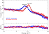 |
Fig. A.1 Example of a spectrum in the iron line region generated with different calibrations. The red spectrum corresponds to events generated applying the RDPHA correction, while the blue spectrum corresponds to the RDCTI correction. |
A.2 Test for pile-up in the iron line region
As mentioned in Sect. 2, our XMM-Newton EPIC-pn observation of Vela X-1 is deeply affected by pile-up. In addition, with the epatplot task, we evaluate the pixel columns most affected by pile-up by performing a test in the iron line region. We extract spectra ignoring 1, 3, 5, and 7 columns from the PSF centre (named PSF–#) and then compare the position of the iron line between different extractions. We present example spectra as in Fig. A.1, using the RDPHA correction (see Fig. A.2) and RDCTI correction (see Fig. A.3), where we fitted with a power law and Gaussian component to model the iron line.
We note that with the RDPHA correction, the more the centremost columns are removed, the lower the energy of the iron line is starting from ~6.54 keV for one column removed to ~6.50 keV for seven ignored columns. However, removing seven columns from the centre of the PSF means ignoring almost the entire available signal, decreasing the S/N. Moreover, the iron line energy is still too high compared to what we expect for this feature as discussed in Sect. A.1. On the contrary, using the RDCTI correction, we obtain the opposite behaviour, with an increase in the iron line energy together with the number of centre columns removed from the PSF. In order to have a good balance between keeping enough signal and having a consistent iron line energy with previous results for Vela X-1, we decided to apply the RDCTI correction and to remove the three centremost columns from the PSF (PSF–3) for this work. Even if we apply those corrections, the energy of the iron line (~6.46 keV) is still higher than what we obtained for the simultaneous NuSTAR observation, and so discrepancies between the two instruments are expected for the combined spectral analysis presented in Sect. 4.2.
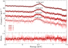 |
Fig. A.2 Example of a spectrum with RDPHA correction as in Fig. A.1, removing 1 (PSF–1), 3 (PSF-3), 5 (PSF-5), and 7 (PSF–7) columns from the centre of the PSF. |
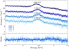 |
Fig. A.3 Example of a spectrum with RDCTI correction as in Fig. A.1 removing 1 (PSF–1), 3 (PSF–3), 5 (PSF–5), and 7 (PSF–7) columns from the centre of the PSF. |
A.3 Cross-instrumental issues
In comparison with XMM-Newton EPIC-pn data, we observe a strong soft excess in the NuSTAR data (see Fig. A.4). A possible explanation for this is the dust scattering effect. In this scenario, we suppose dense interstellar clouds located between the observer and the source. Those clouds will lead to deviation of the trajectory of low-energy photons that were not supposed to be observed. The low-energy photons will then be scattered towards the observer, producing a soft excess flux at low energy in the spectrum of the source. This scattering leads to the formation of the scattering halo as observed in Circinus X-1 in Heinz et al. (2015). To check for this phenomenon, we extracted source regions of different sizes in the NuSTAR data from 10 arcsec to 50 arcsec is steps of 10 arcsec. The smallest source regions account for the maximum of the PSF, though with a possible loss of information from the source. The largest source regions account for the PSF and outside wings, which is where the dust scattering effect is visible and more low-energy photons are present. When comparing the resultant spectra, we cannot see any difference in terms of spectral shape, meaning the soft excess at low energy is always present. Hence, we exclude the dust scattering effect as a cause for the observed soft excess in our NuSTAR data. We also checked for contamination sources in the extracted source region of both instruments but none could be found. As we are unable to find a plausible physical explanation for this phenomenon, we tested our model by tying CFNuSTAR to CFXMN. In the second residual panel of Fig. A.4, we observe that the XMM-Newton EPIC-pn data are well described, albeit the residuals increase drastically for NuSTAR around 3 keV. Reciprocally, we tied CFXMN to CFNuSTAR and, as expected, the NuSTAR data are well constrained. However, there is a discrepancy up to a factor of 10 between the model and the XMM-Newton EPIC-pn data at 0.5 keV as shown on the last residual panel of Fig. A.4. None of the datasets are correctly described by an averaged CF. We conclude that the CFXMN is the most reliable value for the covering fraction and that the problem may be due to remaining calibration effects from NuSTAR at low energies. For the rest of this work, we assumed two independent CFs for each instrument as this is the best way to empirically compensate for the observed difference (see the first residual panel of Fig. A.4). In Tsygankov et al. (2019), an offset between Swift/XRT and NuSTAR has also been reported. The Swift/XRT normalisation was about 1.3 times lower than NuSTAR FPMA/FPMB, which is possibly due to the fact that their NuSTAR and Swift observations were not strictly simultaneous.
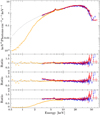 |
Fig. A.4 Example of an unfolded spectrum taken with XMM-Newton EPIC-pn (orange), NuSTAR FPMA (red), and FPMB (blue) during the fourth NuSTAR orbit. Solid lines show the best-fit model with independent CFXMN and CFNuSTAR, and dotted lines account for best-fit model with tied CFs. First residual panel: Best-fit model with independent covering fractions. Second residual panel: Best-fit model with CFNuSTAR tied to CFXMN- Last residual panel: Best-fit model with CFXMN tied to CFNuSTAR- A strong soft excess in the NuSTAR data is visible at ~3 keV in comparison to the XMM-Newton data. |
References
- Amato, R., Grinberg, V., Hell, N., et al. 2021, A&A, 648, A105 [NASA ADS] [CrossRef] [EDP Sciences] [Google Scholar]
- Arnaud, K. A. 1996, ASP Conf. Ser., 101, 17 [Google Scholar]
- Astropy Collaboration (Price-Whelan, A. M., et al.) 2022, ApJ, 935, 167 [NASA ADS] [CrossRef] [Google Scholar]
- Bachetti, M., Huppenkothen, D., Khan, U., et al. 2022, StingraySoftware/ stingray: v1.0-beta [Google Scholar]
- Barret, D., Decourchelle, A., Fabian, A., et al. 2020, Astron. Nachr., 341, 224 [NASA ADS] [CrossRef] [Google Scholar]
- Becker, R. H., Rothschild, R. E., Boldt, E. A., et al. 1978, ApJ, 221, 912 [NASA ADS] [CrossRef] [Google Scholar]
- Bildsten, L., Chakrabarty, D., Chiu, J., et al. 1997, ApJS, 113, 367 [CrossRef] [Google Scholar]
- Blondin, J. M. 1994, AIP Conf. Ser., 308, 578 [Google Scholar]
- Blondin, J. M., Kallman, T. R., Fryxell, B. A., & Taam, R. E. 1990, ApJ, 356, 591 [Google Scholar]
- Blondin, J. M., Stevens, I. R., & Kallman, T. R. 1991, ApJ, 371, 684 [NASA ADS] [CrossRef] [Google Scholar]
- Conti, P. S. 1978, A&A, 63, 225 [NASA ADS] [Google Scholar]
- den Herder, J. W., Brinkman, A. C., Kahn, S. M., et al. 2001, A&A, 365, L7 [NASA ADS] [CrossRef] [EDP Sciences] [Google Scholar]
- Diez, C. M., Grinberg, V., Fürst, F., et al. 2022, A&A, 660, A19 [NASA ADS] [CrossRef] [EDP Sciences] [Google Scholar]
- Drake, G. W. 1988, Can. J. Phys., 66, 586 [Google Scholar]
- El Mellah, I., Grinberg, V., Sundqvist, J. O., Driessen, F. A., & Leutenegger, M. A. 2020, A&A, 643, A9 [NASA ADS] [CrossRef] [EDP Sciences] [Google Scholar]
- Erickson, G. W. 1977, J. Phys. Chem. Ref. Data, 6, 831 [Google Scholar]
- Falanga, M., Bozzo, E., Lutovinov, A., et al. 2015, A&A, 577, A130 [NASA ADS] [CrossRef] [EDP Sciences] [Google Scholar]
- Fransson, C., & Fabian, A. C. 1980, A&A, 87, 102 [NASA ADS] [Google Scholar]
- Fürst, F., Kreykenbohm, I., Pottschmidt, K., et al. 2010, A&A, 519, A37 [CrossRef] [EDP Sciences] [Google Scholar]
- Fürst, F., Suchy, S., Kreykenbohm, I., et al. 2011, A&A, 535, A9 [NASA ADS] [CrossRef] [EDP Sciences] [Google Scholar]
- Fürst, F., Pottschmidt, K., Wilms, J., et al. 2014a, ApJ, 784, L40 [CrossRef] [Google Scholar]
- Fürst, F., Pottschmidt, K., Wilms, J., et al. 2014b, ApJ, 780, 133 [Google Scholar]
- Garcia, J. D., & Mack, J. E. 1965, J. Opt. Soc. Am., 55, 654 [NASA ADS] [CrossRef] [Google Scholar]
- Giménez-García, A., Shenar, T., Torrejón, J. M., et al. 2016, A&A, 591, A26 [EDP Sciences] [Google Scholar]
- Gokus, A. 2017, Master’s thesis, (Universität Erlangen-Nürnberg, Germany) [Google Scholar]
- Goldstein, G., Huenemoerder, D. P., & Blank, D. 2004, AJ, 127, 2310 [Google Scholar]
- Grinberg, V., Hell, N., El Mellah, I., et al. 2017, A&A, 608, A143 [NASA ADS] [CrossRef] [EDP Sciences] [Google Scholar]
- Grinberg, V., Nowak, M. A., & Hell, N. 2020, A&A, 643, A109 [NASA ADS] [CrossRef] [EDP Sciences] [Google Scholar]
- Haberl, F., & White, N. E. 1990, ApJ, 361, 225 [Google Scholar]
- Heinz, S., Burton, M., Braiding, C., et al. 2015, ApJ, 806, 265 [Google Scholar]
- Hell, N., Brown, G. V., Wilms, J., et al. 2016, ApJ, 830, 26 [Google Scholar]
- HI4PI Collaboration (Ben Bekhti, N., et al.) 2016, A&A, 594, A116 [NASA ADS] [CrossRef] [EDP Sciences] [Google Scholar]
- Hiltner, W. A., Werner, J., & Osmer, P. 1972, ApJ, 175, L19 [Google Scholar]
- Hirsch, M., Hell, N., Grinberg, V., et al. 2019, A&A, 626, A64 [NASA ADS] [CrossRef] [EDP Sciences] [Google Scholar]
- Houck, J. C., & Denicola, L. A. 2000, ASP Conf. Ser., 216, 591 [Google Scholar]
- House, L. L. 1969, ApJS, 18, 21 [NASA ADS] [CrossRef] [Google Scholar]
- Huppenkothen, D., Bachetti, M., Stevens, A., et al. 2019a, J. Open Source Softw., 4, 1393 [NASA ADS] [CrossRef] [Google Scholar]
- Huppenkothen, D., Bachetti, M., Stevens, A. L., et al. 2019b, ApJ, 881, 39 [Google Scholar]
- Jansen, F., Lumb, D., Altieri, B., et al. 2001, A&A, 365, L1 [NASA ADS] [CrossRef] [EDP Sciences] [Google Scholar]
- Jethwa, P., Saxton, R., Guainazzi, M., Rodriguez-Pascual, P., & Stuhlinger, M. 2015, A&A, 581, A104 [NASA ADS] [CrossRef] [EDP Sciences] [Google Scholar]
- Joss, P. C., & Rappaport, S. A. 1984, ARA&A, 22, 537 [Google Scholar]
- Kaastra, J. S., & Bleeker, J. A. M. 2016, A&A, 587, A151 [NASA ADS] [CrossRef] [EDP Sciences] [Google Scholar]
- Kallman, T. R., & McCray, R. 1982, ApJS, 50, 263 [NASA ADS] [CrossRef] [Google Scholar]
- Kendziorra, E., Mony, B., Kretschmar, P., et al. 1992, in Frontiers Science Series, eds. Y. Tanaka, & K. Koyama, 51 [Google Scholar]
- Kretschmar, P., Pan, H. C., Kendziorra, E., et al. 1997, A&A, 325, 623 [NASA ADS] [Google Scholar]
- Kretschmar, P., El Mellah, I., Martínez-Núñez, S., et al. 2021, A&A, 652, A95 [NASA ADS] [CrossRef] [EDP Sciences] [Google Scholar]
- Kreykenbohm, I., Kretschmar, P., Wilms, J., et al. 1999, A&A, 341, 141 [NASA ADS] [Google Scholar]
- Kreykenbohm, I., Coburn, W., Wilms, J., et al. 2002, A&A, 395, 129 [NASA ADS] [CrossRef] [EDP Sciences] [Google Scholar]
- Kreykenbohm, I., Wilms, J., Kretschmar, P., et al. 2008, A&A, 492, 511 [NASA ADS] [CrossRef] [EDP Sciences] [Google Scholar]
- Lai, E. V., De Marco, B., Zdziarski, A. A., et al. 2022, MNRAS, 512, 2671 [NASA ADS] [CrossRef] [Google Scholar]
- Lewis, W., Rappaport, S., Levine, A., & Nagase, F. 1992, ApJ, 389, 665 [NASA ADS] [CrossRef] [Google Scholar]
- Lomaeva, M., Grinberg, V., Guainazzi, M., et al. 2020, A&A, 641, A144 [NASA ADS] [CrossRef] [EDP Sciences] [Google Scholar]
- Madsen, K. K., Grefenstette, B. W., Pike, S., et al. 2020, ArXiv e-prints, [arXiv:2005.00569] [Google Scholar]
- Malacaria, C., Mihara, T., Santangelo, A., et al. 2016, A&A, 588, A100 [NASA ADS] [CrossRef] [EDP Sciences] [Google Scholar]
- Manousakis, A., & Walter, R. 2015a, A&A, 575, A58 [NASA ADS] [CrossRef] [EDP Sciences] [Google Scholar]
- Manousakis, A., & Walter, R. 2015b, A&A, 584, A25 [NASA ADS] [CrossRef] [EDP Sciences] [Google Scholar]
- Manousakis, A., Walter, R., & Blondin, J. M. 2012, A&A, 547, A20 [NASA ADS] [CrossRef] [EDP Sciences] [Google Scholar]
- Martínez-Núñez, S., Torrejón, J. M., Kühnel, M., et al. 2014, A&A, 563, A70 [NASA ADS] [CrossRef] [EDP Sciences] [Google Scholar]
- Martínez-Núñez, S., Kretschmar, P., Bozzo, E., et al. 2017, Space Sci. Rev., 212, 59 [Google Scholar]
- Nagase, F., Zylstra, G., Sonobe, T., et al. 1994, ApJ, 436, L1 [NASA ADS] [CrossRef] [Google Scholar]
- Nowak, M. A., Hanke, M., Trowbridge, S. N., et al. 2011, ApJ, 728, 13 [Google Scholar]
- Ohashi, T., Inoue, H., Koyama, K., et al. 1984, PASJ, 36, 699 [NASA ADS] [Google Scholar]
- Orlandini, M., Dal Fiume, D., Frontera, F., et al. 1998, A&A, 332, 121 [NASA ADS] [Google Scholar]
- Pintore, F., Sanna, A., Di Salvo, T., et al. 2014, MNRAS, 445, 3745 [NASA ADS] [CrossRef] [Google Scholar]
- Quaintrell, H., Norton, A. J., Ash, T. D. C., et al. 2003, A&A, 401, 313 [NASA ADS] [CrossRef] [EDP Sciences] [Google Scholar]
- Rawls, M. L., Orosz, J. A., McClintock, J. E., et al. 2011, ApJ, 730, 25 [NASA ADS] [CrossRef] [Google Scholar]
- Sako, M., Liedahl, D. A., Kahn, S. M., & Paerels, F. 1999, ApJ, 525, 921 [Google Scholar]
- Sato, N., Hayakawa, S., Nagase, F., et al. 1986, PASJ, 38, 731 [NASA ADS] [Google Scholar]
- Schulz, N. S., Canizares, C. R., Lee, J. C., & Sako, M. 2002, ApJ, 564, L21 [Google Scholar]
- Staubert, R., Trümper, J., Kendziorra, E., et al. 2019, A&A, 622, A61 [NASA ADS] [CrossRef] [EDP Sciences] [Google Scholar]
- Strüder, L., Briel, U., Dennerl, K., et al. 2001, A&A, 365, L18 [Google Scholar]
- Tiesinga, E., Mohr, P. J., Newell, D. B., & Taylor, B. N. 2021, Rev. Mod. Phys., 93, 025010 [NASA ADS] [CrossRef] [Google Scholar]
- Tsygankov, S. S., Rouco Escorial, A., Suleimanov, V. F., et al. 2019, MNRAS, 483, L144 [NASA ADS] [CrossRef] [Google Scholar]
- Turner, M. J. L., Abbey, A., Arnaud, M., et al. 2001, A&A, 365, L27 [CrossRef] [EDP Sciences] [Google Scholar]
- van Kerkwijk, M. H., van Paradijs, J., & Zuiderwijk, E. J. 1995, A&A, 303, 497 [NASA ADS] [Google Scholar]
- Verner, D. A., Ferland, G. J., Korista, K. T., & Yakovlev, D. G. 1996, ApJ, 465, 487 [Google Scholar]
- Watanabe, S., Sako, M., Ishida, M., et al. 2006, ApJ, 651, 421 [Google Scholar]
- Wilms, J., Allen, A., & McCray, R. 2000, ApJ, 542, 914 [Google Scholar]
- XRISM Science Team 2020, ArXiv e-prints, [arXiv:2003.04962] [Google Scholar]
See the XMM-Newton CCF Release Note 0369 (Migliari S., Smith M., 2019, XMM-CAL-SRN-0369) https://xmmweb.esac.esa.int/docs/documents/CAL-SRN-0369-0-0.pdf
See the XMM-Newton Science Operations Team Calibration Technical Note 0230 (Fürst F., 2022, XMM-SOC-CAL-TN-0230) https://xmmweb.esac.esa.int/docs/documents/CAL-TN-0230-1-3.pdf
see the CCF Release Note 0312 (Guainazzi M., 2014a, XMM-CCF-REL-0312) https://xmmweb.esac.esa.int/docs/documents/CAL-SRN-0312-1-4.pdf and the Science Operations Team Calibration Technical Note 0083 (Guainazzi M., et al. 2014b, XMM-SOC-CAL-TN-0083) https://xmmweb.esac.esa.int/docs/documents/CAL-TN-0083.pdf
All Tables
All Figures
|
Fig. 1 Sketch of Vela X-1 showing the orbital phases covered during this XMM-Newton EPIC-pn observation. In this image, the observer is located facing the system at the bottom of the picture. |
| In the text | |
|
Fig. 2 Light curves for XMM-Newton EPIC-pn (orange), NuSTAR FPMA (red), and FPMB (blue) with a time resolution of P = 283.44 s. The count rate is plotted on the y-axis in logarithmic scale against the orbital phase (top axis) and the time of the observation (bottom axis). Major short flares are indicated by single arrows. The connected arrows at ~58607.42 MJD indicate a flaring episode of ~8 ks. |
| In the text | |
|
Fig. 3 XMM-Newton EPIC-pn spectra extracted during the three different phases of the observation. These are shown in chronological order from the top to the bottom panel: Phase of stable hardness ratio (0.37 ≲ ϕοrb ≲ 0.44), phase of the loss of NuSTAR data (0.44 ≲ ϕοrb ≲ 0.46), and phase of the rise of the hardness ratio (0.46 ≲ ϕorb ≲ 0.51), respectively. The vertical red dashed lines indicate the four energy bands we chose for the extraction of the energy-resolved light curves. |
| In the text | |
|
Fig. 4 Light curves for XMM-Newton EPIC-pn in different energy bands with a time resolution of P = 283.44 s. The count rate shown on the y-axis in logarithmic scale is plotted against the orbital phase and the time of the observation. The energy bands are 0.5−3.0, 3.0–6.0, 6.0–8.0, 8.0–10.0 keV. |
| In the text | |
|
Fig. 5 Light curve and hardness ratios for XMM-Newton EPIC-pn. The first panel shows the overall count rate in the 0.5–10 keV energy band as in Fig. 2. The following panels show the hardness ratios between the mentioned energy bands. The time resolution is Ρ = 283.44 s. |
| In the text | |
|
Fig. 6 XMM-Newton EPIC-pn colour-colour diagram. The data points represent the ratios of the light curves in hard colour depending on soft colour, from beginning (light green) to end (dark green) of the observation. We also show the theoretical expectation for different covering fractions CF (shades of red, varying from 0.97 to 0.99) and absorption column densities NH,1 (shades of blue, varying from 3 × 1022 cm−2 to 80 × 1022 cm−2) using our partial covering model from Eq. (4). We used a photon index Γ of 1.0. More details about the simulation and its interpretation are given in Sect. 5.1.1. |
| In the text | |
|
Fig. 7 Example XMM-Newton EPIC-pn spectrum (black datapoints). We show the last and most absorbed NuSTAR-orbit of our observation. We indicate the individual model components including all lines detected in this dataset (blue dot-dashed Gaussians) and the absorbed continuum (blue dotted line). We refer to Sect. 4.2 for a detailed description of the model and to Table 2 for the soft lines. |
| In the text | |
|
Fig. 8 Results of the NuSTAR-orbit-by-orbit analysis with NuSTAR and XMM-Newton as a function of time, together with the corresponding binary orbital phase. From top to bottom: Photon index (Γ), folding energy (Efold) in keV, energy of the FeKα line in keV, unab-sorbed flux ℱ0.5−78,keV in keV s−1 cm−2, CFs with NuSTAR (CFNuSTAR) and XMM-Newton EPIC-pn (CFXMN), absorption from the stellar wind NH,1 in 1022 cm−2. Circles show data fully covered by both XMM-Newton EPIC-pn and NuSTAR. Triangles show data missing coverage from one of the two instruments. Magenta marks the data only covered by NuSTAR (NuSTAR-orbit 1) and orange the data fully covered by one instrument but partially by the second one (NuSTAR-orbits 10, 11, 14 and 21). Finally, yellow is used to denote data only covered by XMM-Newton EPIC-pn (NuSTAR-orbits 12 and 13). |
| In the text | |
|
Fig. 9 Results of the pulse-by-pulse analysis as a function of time, together with the corresponding binary orbital phase. The panels show (from top to bottom) photon index (Γ), energy of the FeKα line in keV, unabsorbed flux ℱ0.5–10 keV in keV s−1 cm−2, CF with XMM-Newton EPIC-pn (CFXMN), and absorption from the stellar wind NH,1 in 1022 cm−2. |
| In the text | |
|
Fig. 10 Effect of increasing absorption on our model from Eq. (4) with photon index Γ = 1.0 and without emission lines to focus on the evolution of the continuum shape. We assume a CF of 0.9 and a varying absorption column density NH,1 from 3 × 1022 cm−2 to 80 × 1022 cm−2 covering the range obtained in Fig. 9. The shaded grey areas indicate three energy bands of interest: The A band from 0.5 to 3 keV, B band from 3 to 6 keV, and C band from 6 to 10 keV. The resulting observed spectrum (solid lines) is the sum of the spectrum not covered by the stellar wind (dash-dotted line) and the covered spectrum (dashed lines). See Fig. 3 of Diez et al. (2022) for an illustrated picture of the partial covering model. |
| In the text | |
|
Fig. 11 Comparison of the NH values determined in this study with historical measurements taken during individual binary orbits by Tenma (Ohashi et al. 1984) and EXOSAT (Haberl & White 1990). We highlight the overall similar slope of the different rising curves. See text for details. |
| In the text | |
|
Fig. 12 Comparison of the NH values determined in this study with a range of model results for NH from hydrodynamic simulations for Vela X-1 or similar, but not identical model systems. See the main text and Table 3. |
| In the text | |
|
Fig. 13 Fluxes in photons s−1 cm−2 of some soft lines obtained within the pulse-by-pulse analysis as functions of time, together with the corresponding binary orbital phase. The panels show (from top to bottom) the flux of the FeKα, the FeKβ, the Ne IX, and the S XV line. |
| In the text | |
|
Fig. 14 Timing analysis of NH evolution: (a) Stingray average power spectrum; (b) Stingray z-square function; (c) Stingray chi-square function; (d) Astropy v5.1 Lomb-Scargle Periodogram. |
| In the text | |
|
Fig. A.1 Example of a spectrum in the iron line region generated with different calibrations. The red spectrum corresponds to events generated applying the RDPHA correction, while the blue spectrum corresponds to the RDCTI correction. |
| In the text | |
|
Fig. A.2 Example of a spectrum with RDPHA correction as in Fig. A.1, removing 1 (PSF–1), 3 (PSF-3), 5 (PSF-5), and 7 (PSF–7) columns from the centre of the PSF. |
| In the text | |
|
Fig. A.3 Example of a spectrum with RDCTI correction as in Fig. A.1 removing 1 (PSF–1), 3 (PSF–3), 5 (PSF–5), and 7 (PSF–7) columns from the centre of the PSF. |
| In the text | |
|
Fig. A.4 Example of an unfolded spectrum taken with XMM-Newton EPIC-pn (orange), NuSTAR FPMA (red), and FPMB (blue) during the fourth NuSTAR orbit. Solid lines show the best-fit model with independent CFXMN and CFNuSTAR, and dotted lines account for best-fit model with tied CFs. First residual panel: Best-fit model with independent covering fractions. Second residual panel: Best-fit model with CFNuSTAR tied to CFXMN- Last residual panel: Best-fit model with CFXMN tied to CFNuSTAR- A strong soft excess in the NuSTAR data is visible at ~3 keV in comparison to the XMM-Newton data. |
| In the text | |
Current usage metrics show cumulative count of Article Views (full-text article views including HTML views, PDF and ePub downloads, according to the available data) and Abstracts Views on Vision4Press platform.
Data correspond to usage on the plateform after 2015. The current usage metrics is available 48-96 hours after online publication and is updated daily on week days.
Initial download of the metrics may take a while.