| Issue |
A&A
Volume 689, September 2024
|
|
|---|---|---|
| Article Number | A172 | |
| Number of page(s) | 7 | |
| Section | Stellar structure and evolution | |
| DOI | https://doi.org/10.1051/0004-6361/202449228 | |
| Published online | 12 September 2024 | |
XMM-Newton and NuSTAR discovery of a likely IP candidate XMMU J173029.8–330920 in the Galactic disc
1
INAF – Osservatorio Astronomico di Brera, Via E. Bianchi 46, 23807 Merate (LC), Italy
2
Max-Planck-Institut für extraterrestrische Physik, Gießenbachstraße 1, 85748 Garching, Germany
3
Columbia Astrophysics Laboratory, Columbia University, New York, NY 10027, USA
4
School of Astronomy and Space Science, Nanjing University, Nanjing 210046, China
5
Institute of Space Sciences (ICE, CSIC), Campus UAB, Carrer de Can Magrans s/n, E-08193 Barcelona, Spain
6
Institut d’Estudis Espacials de Catalunya (IEEC), Carrer Gran Capità 2–4, 08034 Barcelona, Spain
Received:
13
January
2024
Accepted:
3
July
2024
Abstract
Aims. We aim to characterise the population of low-luminosity X-ray sources in the Galactic plane by studying their X-ray spectra and periodic signals in the light curves.
Methods. We are performing an X-ray survey of the Galactic disc using XMM-Newton, and the source XMMU J173029.8–330920 was serendipitously discovered in our campaign. We performed a follow-up observation of the source using our pre-approved NuSTAR target of opportunity time. We used various phenomenological models in XSPEC for the X-ray spectral modelling. We also computed the Lomb-Scargle periodogram to search for X-ray periodicity. A Monte Carlo method was used to simulate 1000 artificial light curves in order to estimate the significance of the detected period. We also searched for X-ray, optical, and infrared counterparts of the source in various catalogues.
Results. The spectral modelling indicates the presence of an intervening cloud with NH ∼ (1.5 − 2.3)×1023 cm−2 that partially absorbs the incoming X-ray photons. The X-ray spectra are best fit by a model representing emission from a collisionally ionised diffuse gas with a plasma temperature of kT = 26−5+11 keV. Furthermore, an Fe Kα line at 6.47−0.06+0.13 keV was detected with an equivalent width of the line of 312 ± 104 eV. We discovered a coherent pulsation with a period of 521.7 ± 0.8 s. The 3–10 keV pulsed fraction of the source is around ∼50–60%.
Conclusions. The hard X-ray emission with plasma temperature kT = 26−5+11 keV, iron Kα emission at 6.4 keV, and a periodic behaviour of 521.7 ± 0.8 s suggest XMMU J173029.8–33092 to be an intermediate polar. We estimated the mass of the central white dwarf to be 0.94 − 1.4 M⊙ by assuming a distance to the source of ∼1.4 − 5 kpc.
Key words: binaries: close / novae / cataclysmic variables / white dwarfs / Galaxy: center / Galaxy: disk
Corresponding author; This email address is being protected from spambots. You need JavaScript enabled to view it. .
© The Authors 2024
 Open Access article, published by EDP Sciences, under the terms of the Creative Commons Attribution License (https://creativecommons.org/licenses/by/4.0), which permits unrestricted use, distribution, and reproduction in any medium, provided the original work is properly cited.
This article is published in open access under the Subscribe to Open model. This email address is being protected from spambots. You need JavaScript enabled to view it. to support open access publication.
1. Introduction
Galactic X-ray emission is a manifestation of various high-energy phenomena and processes. Studying discrete X-ray sources is essential to understanding stellar evolution, dynamics, end products, and accretion physics. Initial X-ray scans of the Galactic plane have revealed a narrow, continuous ridge of emission, the so-called Galactic ridge X-ray emission (GRXE; Worrall et al. 1982; Warwick et al. 1985), and it extends both sides of the Galactic disc up to ∼40°. A copious amount of 6.7 keV line emission from highly ionised iron was detected from selected regions of the GRXE (Koyama et al. 1989; Yamauchi et al. 1990). The study of the 6.7 keV emission has indicated an optically thin hot plasma distributed mainly along the Galactic plane. The Galactic diffuse X-ray emission can be described by a two-component emission model with a soft temperature of ∼0.8 keV and a hard component of ∼8 keV (Koyama et al. 1996; Tanaka et al. 2000). The origin of the ∼8 keV plasma is less certain. The Galactic potential is too shallow to confine such hot plasma that would escape at a velocity of 1000 km s−1. The Deep Chandra observations of the Galactic Centre (GC) by Wang et al. (2002) (2° ×0.8°) and a region south of the GC (16′×16′) by Revnivtsev et al. (2009) have pointed out that the hard kT ∼ 8 keV diffuse emission is primarily due to unresolved cataclysmic variables (CVs) and active binaries. However, close to the GC (within ±0.8°), a significant diffuse hard X-ray emission was later detected up to energies of 40 keV (Yuasa et al. 2008). In addition, some studies have pointed out that the hard GC emission is truly diffuse by comparing the stellar mass distribution with the Fe XXV (6.7 keV) line intensity map (Uchiyama et al. 2011; Nishiyama et al. 2013; Yasui et al. 2015). A recent study by our group has shown that this diffuse hard emission in the GC can be explained if one assumes the GC stellar population with iron abundances ∼1.9 times higher than those in the Galactic bar/bulge (Anastasopoulou et al. 2023).
Magnetic CVs (mCVs) are categorised into two types based on the magnetic field strength of the white dwarf (WD): intermediate polars (IPs) and polars (see Cropper 1990; Patterson 1994; Mukai 2017). In polars, the magnetic field is strong (> 10 MG) enough to synchronise the spin and orbital period of the system, whereas in IPs, the magnetic field is less strong; therefore, their spin and the orbital period are less synchronised. Most hard X-ray emission from mCVs originates close to the WD surface. The accreting material from the companion star follows the magnetic field lines of the WD, and when approaching the WD polar cap, it reaches a supersonic speed of 3000–10 000 km s−1. A shock front is developed above the star, and the in-falling gas releases its energy in the shock, resulting in hard X-ray photons (Aizu 1973).
The GC region hosts many energetic events, including bubbles and super-bubbles from young and old stars, and various supernovae remnants (Ponti et al. 2015), as well as large-scale structures, such as Galactic chimneys (Ponti et al. 2019, 2021), Fermi bubbles (Su et al. 2010), and eROSITA bubbles (Predehl et al. 2020). Currently, we are performing an X-ray survey of the Galactic disc using XMM-Newton. The main aim of the survey is to constrain the flow of hot baryons that feed the large-scale structures from the GC. The survey region extends from l ≥ 350° to l ≤ 7° and covers a latitude of b ∼ ±1°. The survey has an exposure of 20 ks per tile. During the survey, we detected thousands of X-ray point sources of various types. Our survey is sensitive enough to detect sources as faint as 10−14 erg cm−2 s−1. The nearby bright X-ray point sources with flux > 10−11 erg cm−2 s−1 are well known thanks to several decades of monitoring by RXTE, Swift-BAT, MAXI, and INTEGRAL. The bright IPs in the solar neighbourhood have a typical luminosity of 1033 − 1034 erg s−1 (Downes et al. 2001; Ritter & Kolb 2003; Suleimanov et al. 2022), and its unabsorbed flux at the GC would be ∼10−13 − 10−12 erg cm−2 s−1. Furthermore, the high extinction towards the GC makes it even more difficult to detect these faint sources in the GC. Notably, our XMM-Newton observations are deep enough to detect these faint X-ray sources. During our XMM-Newton campaign, we detected a faint X-ray source, XMMU J173029.8–33092, with a 3–10 keV X-ray luminosity of ∼7 × 10⁻¹³ erg cm−2 s−1. In this paper, we report the detailed spectral and timing study of this source.
2. Observations and data reduction
The source XMMU J173029.8–330920 ( ,
,  ) was discovered in our XMM-Newton (Jansen et al. 2001) Heritage survey of the inner Galactic disc (PI: G. Ponti). The source was detected in one of our XMM-Newton pointings on 2023 March 28 (ObsID: 0916800201) with an exposure of 18.3 ks (Mondal et al. 2024). We analysed the XMM-Newton data and discovered an X-ray pulsation and a tentative iron 6.4 keV line emission that suggested a possible identification with an IP. To confirm this, we triggered our pre-approved 35 ks NuSTAR target of opportunity observation to follow up on this source.
The XMM-Newton observation data file was processed using XMM-Newton Science Analysis System (SASv19.0.01). The point source detection and source list creation were performed using the SAS task emldetect. The source detection was performed simultaneously in five energy bands (0.2–0.5 keV, 0.5–1 keV, 1–2 keV, 2–4 keV, and 4–12 keV) for each detector EPIC-pn/MOS1/MOS2 (Strüder et al. 2001; Turner et al. 2001). While extracting the source products, we only selected the events with PATTERN ≤ 4 and PATTERN ≤ 12 for EPIC-pn and MOS2 detectors, respectively. The source was out of the field of view of the MOS1 detector. We applied a barycentre correction for light curve extraction using the SAS task barycen. We used a circular region of 25″ radius for the source product extraction. The background products were extracted from a nearby source-free circular region of radius 25″.
The NuSTAR (Harrison et al. 2013) observation was performed on 2023 April 24 (ObsID: 80801332002, PI: S. Mondal). The NuSTAR data reduction was performed using the NuSTAR data analysis pipeline software (NUSTARDAS v0.4.9 provided with HEASOFT). The unfiltered event files from the FMPA and FPMB detectors were cleaned, and data taken during passages through the South Atlantic Anomaly were removed using nupipeline. The source products were extracted from a circular region of radius 40″ using nuproducts. The background was selected from a source-free region of 40″ radius.
3. Results
3.1. XMM-Newton and NuSTAR joint spectral modelling
We performed time-averaged spectral modelling using XSPEC (Arnaud 1996), including the data from the EPIC-pn, MOS2, FPMA, and FPMB detectors in a joint fit. While doing the fit, we added a constant term for cross-calibration uncertainty, which we fixed at unity for the EPIC-pn detector and left free for the others. The best-fit parameters are listed in Table 1, and the quoted errors are at the 90% confidence level. All the models were convolved with a Galactic absorption component tbabs (Wilms et al. 2000) with solar abundance.
Best-fit parameters of the fitted models.
Before we started fitting the data from XMM-Newton and NuSTAR jointly, we checked for any variation in flux, as the two observations are separated by nearly 27 days. We chose a common energy band of 3–10 keV in XMM-Newton and NuSTAR to estimate the flux and fit the spectra using a simple power-law model. The power-law model provides 3–10 keV flux in XMM-Newton and NuSTAR is  and
and  , respectively. As we did not see any indication of flux variation, we jointly modelled the spectra from XMM-Newton and NuSTAR. First, we fitted the data with an absorbed power law model that leads to a high NH = (16 ± 3) × 1022 cm−2 and Γ = 1.9 ± 0.2. Fitting the data with this model revealed residuals at energies below 3 keV. The partial covering component improved the fit by Δχ2 = 17 for two additional degrees of freedom (d.o.f.). The significance of the partial covering component is 99.84% in an F-test. The fitted parameters are
  ,
,  ,
,  , and Γ = 2.1 ± 0.2. Next, we added a Gaussian that further improved the fit by Δχ2 = 13 for an additional one d.o.f. that gives a detection significance of 99.90% in an F-test. The line width was consistent with zero; therefore, we set the line width to 0 keV, and we estimated the centroid of the line as
  keV. The equivalent width of the line is 312 ± 104 eV. We checked the presence of Fe XXV and Fe XXVI by adding two Gaussians at 6.7 and 6.9 keV; however, there was no significant improvement in the fit. The best fit was obtained when the data was fitted with an absorbed apec model representing the emission from collisionally ionised diffuse gas. The apec model does not include the neutral Fe Kα emission at 6.4 keV. Therefore, we added a Gaussian at 6.4 keV when fitting with this model. The plasma temperature we obtained from this model is
  keV.
keV.
3.2. X-ray pulsation search
For a primary analysis and search for X-ray pulsation in XMM-Newton EPIC-pn and NuSTAR FPMA detectors, we chose a common energy band 3–10 keV to extract the light curve. The X-ray light curves often suffer from gaps due to the South Atlantic Anomaly passage. The gaps in the light curve are prominent for satellites in low Earth orbit such as NuSTAR due to Earth occultation. We used the Lomb-Scargle (Lomb 1976) periodogram to search for periodicity. The Lomb-Scargle periodogram is well known for detecting periodicity in observations that suffer from gaps. Figure 2 shows the Lomb-Scargle periodogram for the EPIC-pn and FPMA detectors. A peak at around a frequency of 1.918 × 10⁻³ Hz and 1.916 × 10⁻³ Hz is visible in the EPIC-pn and FPMA detectors, respectively. The periods obtained from the EPIC-pn and FPMA data are 521.2 ± 3.6 and 521.7 ± 0.8, respectively; both are consistent with each other.
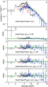 |
Fig. 1. Spectra of XMMU J173029.8–330920 fitted with various partially absorbed models plus a Gaussian component at ∼6.4 keV. The black, red, green, and blue data points are from EPIC-pn, MOS2, FPMA, and FPMB detectors; tbabs and tbpcf represent the Galactic and partial absorption component; and po (a simple power law) and apec (a collisionally ionised diffuse gas) are the two continuum models tested in the spectral modelling. More details are given in Sect. 3.1. |
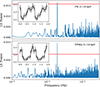 |
Fig. 2. Lomb-Scargle periodogram of the source XMMU J173029.8–330920. The top panel is for data from the XMM-Newton EPIC-pn detector, and the bottom panel is for the NuSTAR FPMA detector. In both cases, a significant peak around 1.918 × 10⁻³ Hz is visible, which corresponds to the period of 521 s. The small insects show the 3–10 keV folded light curve. The red horizontal lines indicate the 3σ detection significance. |
The periodogram of accreting X-ray binaries displays red noise, which can mimic an artificial periodic or aperiodic variability. Therefore, we performed Monte Carlo simulations to test the detection significance. To begin, we computed the power spectral density (PSD) using the standard periodogram approach with an [rms/mean]2 PSD normalisation (Vaughan et al. 2003). Subsequently, we employed a power-law model to characterise the source power spectrum while taking into account the presence of red noise. The power law model is expressed as
 (1)
(1)
where N represents the normalisation factor and Cp accounts for the Poisson noise, which is influenced by the mean photon flux of the source. We fitted the PSD of the source using Eq. (1) with a Markov chain Monte Carlo approach, employing the Python package emcee (Foreman-Mackey et al. 2013) to derive the best-fit parameters and their associated uncertainties. We simulated 1000 light curves for this best-fit power law model using the method of Timmer & Koenig (1995), which were re-sampled and binned to have the same duration, mean count rate, and variance as the observed light curve. The red horizontal lines in Fig. 2 indicate the 3σ detection significance.
The 3–10 keV pulsed fractions (PFs) obtained from EPIC-pn and FPMA are 50.4 ± 15.5 and 59.3 ± 14.7, respectively. The PF was calculated by using the formula  , where Fmax and Fmin are the normalised count of the folded light curve. Next, we computed the PF of the source at different energies. Figure 3 shows the pulsed fraction at different energies. The 0.5–5 keV and 5–10 keV pulse fraction is 55 ± 17% and 42 ± 16%, respectively.
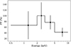 |
Fig. 3. Pulsed fractions of the source as a function of energy. The error bars of the pulse fractions have a 1σ confidence level. |
4. Counterparts
We searched for X-ray counterparts in the Chandra CSC2.02 and Swift 2SXPS3 catalogues; however, no counterparts were found. We searched for optical and infrared counterparts in various catalogues, and no Gaia counterpart was found within 5″ from the XMM-Newton position due to high interstellar medium absorption. A source was found in the VVV Infrared Astrometric Catalogue (Smith et al. 2018); however, the source is located 2.7″ away from the XMM-Newton position, which is off by more than 3σ (1″) XMM-Newton positional uncertainty, so we considered that no infrared counterparts were detected. From the observed column density of absorption of  , we estimated the distance to the source by comparing this value to the absorption column density obtained from several other tracers (Planck Collaboration Int. XLVIII 2016; Yao et al. 2017; Edenhofer et al. 2024). Assuming that all the observed column density in the X-ray band is due to interstellar absorption, we obtained the distance to the source as being around
  kpc using the 3D-NH-tool4 of Doroshenko (2024). In any case, the source should be closer to Earth than 5 kpc.
From the non-detections in the VVV and Gaia data, we could put a constraint on the nature of the companion star. The extinction along the line of sight in the optical and infrared band is AV = 6.36 and AK = 0.61, respectively (Doroshenko 2024). The Gaia G band and VVV infrared survey have a detection limit of mG = 21 and mKs = 18.1, respectively. Therefore, we established that the absolute magnitude of the donor star should be MG > 2.3 and MKs > 5.1. The donor star might be even fainter than the above estimates, as the optical emission from this type of system has a significant contribution from the accretion disc (Mukai & Pretorius 2023). Therefore, the upper limits of the optical and infrared magnitude suggest that the companion star should be a low-mass main-sequence star of a spectra type later than A7/F0. Our XMM-Newton observation has simultaneous UV observation with UVW1 (291 nm) and UVM2 (231 nm) filters. We did not find any counterparts in the XMM-Newton UV data.
5. Discussion
The source XMMU J173029.8–330920 was discovered in March 2023 during our XMM-Newton campaign. Shortly afterwards, in April of 2023, we triggered our pre-allocated NuSTAR observation to follow up on this source. We searched for a counterpart in the Swift and Chandra source catalogues but found no source association. We also looked for optical, infrared counterparts in the Gaia and 2MASS catalogues, but no counterparts were found.
When we fit the X-ray spectra of the source with a single Galactic absorption component, that leaves residual in the ratio plot. The X-ray spectra are best fitted when we incorporate a partial covering component into the spectral models. The partial covering absorber has a column density of NH, pcf = (1.5 − 2.3)×1023 cm−2. The requirement of a partial covering is commonly seen in the spectra of magnetic CVs (Ezuka & Ishida 1999; Mondal et al. 2022, 2023). A partial covering absorption suggests a fraction of the photons are seen directly, while the rest are seen through an intervening absorber, which suggests the absorber size is of the same order as the X-ray emitting region located closer to the source. A simple absorber with a column density of 1023 cm−2 is so high that it completely absorbs the photons below 2 keV, yet most IPs show a good level of emission in the soft X-ray band 0.2–2 keV. Therefore, Norton & Watson (1989) introduced the concept of a partial covering absorber that improved the spectral fit and explained the observed energy-dependent spin modulation. The total hydrogen absorption column density (HI+H2)5 along the line of sight is NHI + H2 = 1.4 × 1022 cm−2 (Willingale et al. 2013). The Galactic absorption towards the source obtained from X-ray spectral fitting is (2 − 3)×1022 cm−2, which is slightly higher than the total hydrogen absorption column density along the line of sight NHI + H2.
A pulsation period of 521.7 ± 0.8 s was found in both the XMM-Newton and NuSTAR data sets. The period is likely to be associated with the spin period of the WD. Such a spin period is typical for an IP. Typically, the spin period of IPs ranges from ∼30 s to ∼3000 s, with a median value around ∼1000 s (Scaringi et al. 2010). The high energy 5–10 keV pulsed fraction of the source is 42 ± 16%. The PF in IPs decreases with increasing energy. This is due to the fact that the light curve of IPs shows increasing modulation depth with decreasing energy (Norton & Watson 1989), and photoelectric absorption has been considered in some part responsible for this trend. Most IPs do not show a large PF at higher energies; however, the sources GK Per (Norton & Watson 1989), AO Psc, and FO Aqr (Hellier et al. 1993) show PFs of the order of 25–35% at energies above 5 keV, which is similar to the PF detected in the 5–10 keV band for the source XMMU J173029.8–330920.
The source is most likely a strong candidate for being an IP. The upper limit estimates of the optical and infrared magnitude indicate the source is hosting a low-mass companion star. The optical extinction of AV = 6.36 along the line of sight is not high enough for non-detection of the optical/infrared counterpart if the source contains a high-mass companion, therefore ruling out the neutron star high-mass X-ray binary (NS HMXRB) scenario. Furthermore, the source spectrum is extremely soft, with Γ ∼ 1.9, which is not typically seen in NS HMXRBs. The NS HMXRBs do not show strong ionised 6.7 and 6.9 keV lines, and their spectra are best fitted by an absorbed power-law model. On the other hand, the spectra of the source XMMU J173029.8–330920 are best fitted by an apec model that is typically used for fitting the spectra of IPs. Lastly, the source is also unlikely to be an ultra-compact X-ray binary (UCXB). The UCXBs are low-mass X-ray binaries usually containing a WD donor and a neutron star accretor with an ultra-short orbital period (< 1 h). The emission from NS-UCXBs is well characterised by black-body emission, with kT ∼ 1 − 3 keV originating from the NS surface (Koliopanos 2015). In our case, a black-body component does not fit the XMM-Newton+NuSTAR 0.5–50 keV spectrum and leaves excess above 10 keV in the ratio plot. Furthermore, a partial covering model is still required when fitting with the black-body model, which is not typically seen when fitting the spectra of NS-UCXB. In addition to that, the NS-UCXBs show little to no emission of Fe (Koliopanos et al. 2021).
5.1. White dwarf mass measurement
As J1730 is an IP whose X-ray emission primarily originates from an accretion column, we measured the WD mass fitting MCVSPEC to the broadband X-ray spectra. First introduced in Vermette et al. (2023), MCVSPEC is an XSPEC spectral model developed for magnetic CVs assuming a magnetically confined 1D accretion flow. Largely based on the methodology of Saxton et al. (2005), MCVSPEC computes the plasma temperature and density profiles varying along the accretion column between the WD surface and shock height. The model outputs an X-ray spectrum with thermal bremsstrahlung continuum and atomic lines by integrating X-ray emissivity over the accretion column. The input parameters for MCVSPEC are M; ṁ (specific accretion rate [g cm−2 s−1]); Rm/R, where Rm is the magnetospheric radius and R is the WD radius; and Z (abundance relative to the solar value).
For IPs where the accretion disc is truncated by WD magnetic fields, we assumed that the free-falling gas gains kinetic energy from the magnetospheric radius (Rm) to the shock height (h). At the shock height, the infalling gas velocity reaches  , which exceeds the sound speed and forms a stand-off shock. As the shock temperature is directly related to M through
  , both Rm and h affect the X-ray spectrum from the accretion column. In addition to MCVSPEC, we incorporated the reflect, Gaussian, and pcfabs models in XSPEC to account for X-ray reflection by the WD surface and X-ray absorption by the accretion curtain. We froze a Gaussian line component for the Fe K-α fluorescent line at 6.4 keV, with a fixed width of σ = 0.01 keV. For the reflect model, we linked the reflection scaling factor (rrefl) to the shock height h, which was determined self-consistently by the MCVSPEC model in each spectral fit following the recipe suggested by Tsujimoto et al. (2018). We note that X-ray reflection is more pronounced when the accretion column is shorter. Overall, the full spectral model was set to tbabs*pcfabs*(reflect*MCVSPEC + gauss).
Before fitting the X-ray spectra, we constrained the range of input parameters, such as Rm/R and ṁ. Following Shaw et al. (2020), we constrained Rm/R by assuming that the WD is in spin equilibrium with the accretion disc at the magnetospheric radius. In this case, the magnetospheric radius is given by  , where P = 521 s is the WD spin period. The specific accretion rate, however, is largely unconstrained due to the unknown source distance (d) and fractional accretion column area (f). The specific accretion rate is defined as
  , where Ṁ is the total mass accretion rate [g s−1]. Assuming that X-ray emission represents most of the radiation from the IP (i.e. L ≈ LX), Ṁ can be calculated from
  , where L = 4πd2FX is the total luminosity and FX represents the unabsorbed X-ray flux. We assumed d = 1.4 − 5 kpc, which is estimated from the Galactic absorption column density towards the line of sight from X-ray spectral fitting. We first estimated the minimum specific accretion rate ṁmin by assuming the shortest source distance (1.4 kpc) and maximum fractional accretion column area (fmax). The fractional accretion column area
  is given for a dipole B-field geometry, assuming that the infalling gas originates from the entire accretion disc truncated at Rm (Frank et al. 2002).
Since some of the parameters described above depend on the WD mass, we adopted a handful of M values, namely, 0.6, 0.8, 0.9, 1.0, 1.1, 1.2, 1.3, and 1.35 M⊙, as initial estimates. For each WD mass estimate, we computed Rm/R and the ṁmin. We then proceeded to fit the X-ray spectra by inputting these Rm/R and the ṁmin values. This is not sufficient since the specific accretion rate may be larger than ṁmin due to a potentially larger source distance (d ≳ 1.4 kpc), smaller fractional accretion column area (f ≲ fmax), and missing source luminosity below the X-ray band (L ≳ LX). Therefore, we also considered a large range of ṁ above ṁmin (ṁ = 0.0043 − 83 [g cm−2 s−1]). For each ṁ value (frozen), we fitted the X-ray spectra and determined the WD mass and statistical errors. We found that the fitted WD mass becomes saturated and independent of ṁ at higher ṁ values (typically ≳10 [g cm−2 s−1]) when the shock height becomes only a small fraction of the WD radius. This saturation of the WD mass over ṁ results from the fact that both the shock temperature and X-ray reflection (both of which are functions of h/R) become less dependent on the shock height.
In each case, our model was well fitted to the X-ray spectra with reduced χ2 = 1.18 − 1.21 (Fig. 4). In the end, we checked the self-consistency of our fitting results by ensuring the measured WD mass was consistent with the assumed WD mass within statistical and systematic errors. The same method was applied to fit broad-band X-ray spectra of another IP obtained by XMM-Newton and NuSTAR (Salcedo & Mori 2024). The systematic errors stem from the range of the specific accretion rate we considered. We found that the initial mass estimates of M ≥ 1.0 M⊙ yielded self-consistent WD mass measurements. We were able to constrain the WD mass range to 0.94 − 1.4 M⊙, which is comparable to or larger than the mean WD mass of magnetic CVs ( ; Pala et al. 2022). The large WD mass range is due to statistical and systematic errors largely associated with the unknown source distance and fractional accretion column area. As emphasised in Vermette et al. (2023), in order to determine the WD mass more accurately in the future, constraining the source distance well and obtaining better photon statistics (particularly above 10 keV) is desirable.
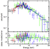 |
Fig. 4. XMM-Newton and NuSTAR spectra of XMMU J173029.8–330920 fit with tbabs*pcfabs*(reflect*MCVSPEC + gauss). This fit utilised an initial mass of 1.2 M⊙ and thus an Rm/R ratio of 26. The specific accretion rate for this fitting was 15 [g cm−2 s−1], resulting in the best-fit WD mass of |
5.2. Fe-K-α lines
There is an indication of Fe Kα line emission at 6.4 keV. The equivalent width of the line is 312 ± 104 eV. Most IP-type sources also display the presence of ionised Fe lines at 6.7 (Fe XXV) and 6.9 (Fe XXVI) keV with an equivalent width higher than 50 eV (Xu et al. 2016). We checked for the presence of the 6.7 and 6.9 keV lines and estimated an upper limit on the equivalent width. The upper limits on the equivalent width of the Fe XXV and Fe XXVI lines are 134 and 147 eV, respectively, which can be confirmed in the future with a longer observation. The 6.4 keV iron Kα line is mainly created by irradiation of neutral material by hard X-ray photons. Compact objects accreting matter through the accretion disc show X-ray reflection from the accretion disc, whereas in the case of accreting WD, most of the hard X-rays are produced so close to the compact object that one might expect half of the photons to be directed towards the WD surface and reflected back to the observer. X-ray reflection in accreting compact objects shows the signature of the Fe Kα fluorescence line and a Compton reflection hump in 10–30 keV. The Compton reflection hump was originally difficult to measure; however, with the launch of the NuSTAR satellite, X-ray reflection has been detected in a couple of magnetic CVs (Mukai et al. 2015). We also checked for the presence of a reflection component in the X-ray spectrum of XMMU J173029.8–33092 by adding a convolution term reflect (Magdziarz & Zdziarski 1995) to the total model. However, the addition of the reflection component did not provide any improvement in Δχ2. On the other hand, the neutral Fe Kα line could have been produced by reprocessing when the hard X-ray passes through the partial covering medium. The hard X-rays travelling through the absorbing material will interact with the iron and create an Fe Kα fluorescence line. In such a scenario, the intensity of the Fe Kα line will increase with the thickness of the ambient material. In a sample study of mCVs using Suzaku data, the column density of the partial absorber seems to correlate with the 6.4 keV line intensity (Eze 2014, 2015), which indicates that the emission of the neutral iron Kα is primarily caused by absorption-induced fluorescence from the absorber.
6. Conclusions
We serendipitously discovered the source XMMU J173029.8–330920 during our XMM-Newton Heritage survey of the Galactic disc. Later, we followed up on the sources using our pre-approved NuSTAR ToO observation. We suggest that the identity of XMMU J173029.8–330920 is an IP based on XMM-Newton and NuSTAR data analysis. The X-ray spectra can be fitted by emission from collisionally ionised diffuse gas with a plasma temperature of  keV. In order to model the X-ray spectrum, one requires a partial covering absorption in addition to the Galactic absorption. The X-ray spectra show the presence of a neutral Fe Kα emission line at 6.4 keV, while the X-ray light curves show periodic modulation with a period of 521.7 ± 0.8 s. These features are commonly seen in accreting magnetic CVs of the IP type.
Acknowledgments
SM and GP acknowledge financial support from the European Research Council (ERC) under the European Union’s Horizon 2020 research and innovation program HotMilk (grant agreement No. 865637). SM and GP also acknowledge support from Bando per il Finanziamento della Ricerca Fondamentale 2022 dell’Istituto Nazionale di Astrofisica (INAF): GO Large program and from the Framework per l’Attrazione e il Rafforzamento delle Eccellenze (FARE) per la ricerca in Italia (R20L5S39T9). KM is partially supported by NASA ADAP program (NNH22ZDA001N-ADAP).
References
- Aizu, K. 1973, Progr. Theoret. Phys., 49, 1184 [NASA ADS] [CrossRef] [Google Scholar]
- Anastasopoulou, K., Ponti, G., Sormani, M. C., et al. 2023, A&A, 671, A55 [NASA ADS] [CrossRef] [EDP Sciences] [Google Scholar]
- Arnaud, K. A. 1996, ASP Conf. Ser., 101, 17 [Google Scholar]
- Cropper, M. 1990, Space Sci. Rev., 54, 195 [CrossRef] [Google Scholar]
- Doroshenko, V. 2024, A&A, submitted [arXiv:2403.03127] [Google Scholar]
- Downes, R. A., Webbink, R. F., Shara, M. M., et al. 2001, PASP, 113, 764 [Google Scholar]
- Edenhofer, G., Zucker, C., Frank, P., et al. 2024, A&A, 685, A82 [NASA ADS] [CrossRef] [EDP Sciences] [Google Scholar]
- Eze, R. N. C. 2014, MNRAS, 437, 857 [NASA ADS] [CrossRef] [Google Scholar]
- Eze, R. N. C. 2015, New Astron., 37, 35 [NASA ADS] [CrossRef] [Google Scholar]
- Ezuka, H., & Ishida, M. 1999, ApJS, 120, 277 [NASA ADS] [CrossRef] [Google Scholar]
- Foreman-Mackey, D., Hogg, D. W., Lang, D., & Goodman, J. 2013, PASP, 125, 306 [Google Scholar]
- Frank, J., King, A., & Raine, D. J. 2002, Accretion Power in Astrophysics, 3rd edn. (Cambridge: Cambridge University Press) [Google Scholar]
- Harrison, F. A., Craig, W. W., Christensen, F. E., et al. 2013, ApJ, 770, 103 [Google Scholar]
- Hellier, C., Garlick, M. A., & Mason, K. O. 1993, MNRAS, 260, 299 [NASA ADS] [CrossRef] [Google Scholar]
- Jansen, F., Lumb, D., Altieri, B., et al. 2001, A&A, 365, L1 [NASA ADS] [CrossRef] [EDP Sciences] [Google Scholar]
- Koliopanos, F. 2015, PhD Thesis, Ludwig-Maximilians University of Munich, Germany [Google Scholar]
- Koliopanos, F., Péault, M., Vasilopoulos, G., & Webb, N. 2021, MNRAS, 501, 548 [Google Scholar]
- Koyama, K., Awaki, H., Kunieda, H., Takano, S., & Tawara, Y. 1989, Nature, 339, 603 [NASA ADS] [CrossRef] [Google Scholar]
- Koyama, K., Maeda, Y., Sonobe, T., et al. 1996, PASJ, 48, 249 [Google Scholar]
- Lomb, N. R. 1976, Ap&SS, 39, 447 [Google Scholar]
- Magdziarz, P., & Zdziarski, A. A. 1995, MNRAS, 273, 837 [Google Scholar]
- Mondal, S., Ponti, G., Haberl, F., et al. 2022, A&A, 666, A150 [NASA ADS] [CrossRef] [EDP Sciences] [Google Scholar]
- Mondal, S., Ponti, G., Haberl, F., et al. 2023, A&A, 671, A120 [NASA ADS] [CrossRef] [EDP Sciences] [Google Scholar]
- Mondal, S., Ponti, G., Bao, T., et al. 2024, A&A, 686, A125 [NASA ADS] [CrossRef] [EDP Sciences] [Google Scholar]
- Mukai, K. 2017, PASP, 129, 062001 [Google Scholar]
- Mukai, K., & Pretorius, M. L. 2023, MNRAS, 523, 3192 [Google Scholar]
- Mukai, K., Rana, V., Bernardini, F., & de Martino, D. 2015, ApJ, 807, L30 [NASA ADS] [CrossRef] [Google Scholar]
- Nishiyama, S., Yasui, K., Nagata, T., et al. 2013, ApJ, 769, L28 [Google Scholar]
- Norton, A. J., & Watson, M. G. 1989, MNRAS, 237, 715 [NASA ADS] [CrossRef] [Google Scholar]
- Pala, A. F., Gänsicke, B. T., Belloni, D., et al. 2022, MNRAS, 510, 6110 [NASA ADS] [CrossRef] [Google Scholar]
- Patterson, J. 1994, PASP, 106, 209 [Google Scholar]
- Planck Collaboration Int. XLVIII. 2016, A&A, 596, A109 [NASA ADS] [CrossRef] [EDP Sciences] [Google Scholar]
- Ponti, G., Morris, M. R., Terrier, R., et al. 2015, MNRAS, 453, 172 [Google Scholar]
- Ponti, G., Hofmann, F., Churazov, E., et al. 2019, Nature, 567, 347 [Google Scholar]
- Ponti, G., Morris, M. R., Churazov, E., Heywood, I., & Fender, R. P. 2021, A&A, 646, A66 [NASA ADS] [CrossRef] [EDP Sciences] [Google Scholar]
- Predehl, P., Sunyaev, R. A., Becker, W., et al. 2020, Nature, 588, 227 [CrossRef] [Google Scholar]
- Revnivtsev, M., Sazonov, S., Churazov, E., et al. 2009, Nature, 458, 1142 [Google Scholar]
- Ritter, H., & Kolb, U. 2003, A&A, 404, 301 [NASA ADS] [CrossRef] [EDP Sciences] [Google Scholar]
- Salcedo, C., & Mori, K. 2024, ApJ, submitted [Google Scholar]
- Saxton, C. J., Wu, K., Cropper, M., & Ramsay, G. 2005, MNRAS, 360, 1091 [NASA ADS] [CrossRef] [Google Scholar]
- Scaringi, S., Bird, A. J., Norton, A. J., et al. 2010, MNRAS, 401, 2207 [NASA ADS] [CrossRef] [Google Scholar]
- Shaw, A. W., Heinke, C. O., Mukai, K., et al. 2020, MNRAS, 498, 3457 [NASA ADS] [CrossRef] [Google Scholar]
- Smith, L. C., Lucas, P. W., Kurtev, R., et al. 2018, MNRAS, 474, 1826 [Google Scholar]
- Strüder, L., Briel, U., Dennerl, K., et al. 2001, A&A, 365, L18 [Google Scholar]
- Su, M., Slatyer, T. R., & Finkbeiner, D. P. 2010, ApJ, 724, 1044 [Google Scholar]
- Suleimanov, V. F., Doroshenko, V., & Werner, K. 2022, MNRAS, 511, 4937 [NASA ADS] [CrossRef] [Google Scholar]
- Tanaka, Y., Koyama, K., Maeda, Y., & Sonobe, T. 2000, PASJ, 52, L25 [NASA ADS] [CrossRef] [Google Scholar]
- Timmer, J., & Koenig, M. 1995, A&A, 300, 707 [NASA ADS] [Google Scholar]
- Tsujimoto, M., Morihana, K., Hayashi, T., & Kitaguchi, T. 2018, PASJ, 70, 109 [NASA ADS] [Google Scholar]
- Turner, M. J. L., Abbey, A., Arnaud, M., et al. 2001, A&A, 365, L27 [CrossRef] [EDP Sciences] [Google Scholar]
- Uchiyama, H., Nobukawa, M., Tsuru, T., Koyama, K., & Matsumoto, H. 2011, PASJ, 63, S903 [NASA ADS] [CrossRef] [Google Scholar]
- Vaughan, S., Edelson, R., Warwick, R. S., & Uttley, P. 2003, MNRAS, 345, 1271 [Google Scholar]
- Vermette, B., Salcedo, C., Mori, K., et al. 2023, ApJ, 954, 138 [NASA ADS] [CrossRef] [Google Scholar]
- Wang, Q. D., Gotthelf, E. V., & Lang, C. C. 2002, Nature, 415, 148 [NASA ADS] [CrossRef] [Google Scholar]
- Warwick, R. S., Turner, M. J. L., Watson, M. G., & Willingale, R. 1985, Nature, 317, 218 [NASA ADS] [CrossRef] [Google Scholar]
- Willingale, R., Starling, R. L. C., Beardmore, A. P., Tanvir, N. R., & O’Brien, P. T. 2013, MNRAS, 431, 394 [Google Scholar]
- Wilms, J., Allen, A., & McCray, R. 2000, ApJ, 542, 914 [Google Scholar]
- Worrall, D. M., Marshall, F. E., Boldt, E. A., & Swank, J. H. 1982, ApJ, 255, 111 [Google Scholar]
- Xu, X.-J., Wang, Q. D., & Li, X.-D. 2016, ApJ, 818, 136 [NASA ADS] [CrossRef] [Google Scholar]
- Yamauchi, S., Kawada, M., Koyama, K., et al. 1990, ApJ, 365, 532 [Google Scholar]
- Yao, J. M., Manchester, R. N., & Wang, N. 2017, ApJ, 835, 29 [NASA ADS] [CrossRef] [Google Scholar]
- Yasui, K., Nishiyama, S., Yoshikawa, T., et al. 2015, PASJ, 67, 123 [NASA ADS] [CrossRef] [Google Scholar]
- Yuasa, T., Tamura, K.-I., Nakazawa, K., et al. 2008, PASJ, 60, S207 [NASA ADS] [CrossRef] [Google Scholar]
All Tables
All Figures
|
Fig. 1. Spectra of XMMU J173029.8–330920 fitted with various partially absorbed models plus a Gaussian component at ∼6.4 keV. The black, red, green, and blue data points are from EPIC-pn, MOS2, FPMA, and FPMB detectors; tbabs and tbpcf represent the Galactic and partial absorption component; and po (a simple power law) and apec (a collisionally ionised diffuse gas) are the two continuum models tested in the spectral modelling. More details are given in Sect. 3.1. |
| In the text | |
|
Fig. 2. Lomb-Scargle periodogram of the source XMMU J173029.8–330920. The top panel is for data from the XMM-Newton EPIC-pn detector, and the bottom panel is for the NuSTAR FPMA detector. In both cases, a significant peak around 1.918 × 10⁻³ Hz is visible, which corresponds to the period of 521 s. The small insects show the 3–10 keV folded light curve. The red horizontal lines indicate the 3σ detection significance. |
| In the text | |
|
Fig. 3. Pulsed fractions of the source as a function of energy. The error bars of the pulse fractions have a 1σ confidence level. |
| In the text | |
|
Fig. 4. XMM-Newton and NuSTAR spectra of XMMU J173029.8–330920 fit with tbabs*pcfabs*(reflect*MCVSPEC + gauss). This fit utilised an initial mass of 1.2 M⊙ and thus an Rm/R ratio of 26. The specific accretion rate for this fitting was 15 [g cm−2 s−1], resulting in the best-fit WD mass of |
| In the text | |
Current usage metrics show cumulative count of Article Views (full-text article views including HTML views, PDF and ePub downloads, according to the available data) and Abstracts Views on Vision4Press platform.
Data correspond to usage on the plateform after 2015. The current usage metrics is available 48-96 hours after online publication and is updated daily on week days.
Initial download of the metrics may take a while.