| Issue |
A&A
Volume 686, June 2024
|
|
|---|---|---|
| Article Number | A125 | |
| Number of page(s) | 18 | |
| Section | Galactic structure, stellar clusters and populations | |
| DOI | https://doi.org/10.1051/0004-6361/202449527 | |
| Published online | 04 June 2024 | |
Periodicity from X-ray sources within the inner Galactic disk
1
INAF – Osservatorio Astronomico di Brera, Via E. Bianchi 46, 23807 Merate (LC), Italy
e-mail: This email address is being protected from spambots. You need JavaScript enabled to view it.
2
Max-Planck-Institut für extraterrestrische Physik, Gießenbachstraße 1, 85748 Garching, Germany
3
School of Astronomy and Space Science, Nanjing University, Nanjing 210046, PR China
4
Columbia Astrophysics Laboratory, Columbia University, Columbia, NY 10027, USA
5
INAF – Istituto di Astrofisica Spaziale e Fisica Cosmica, via A. Corti 12, 20133 Milano, Italy
6
Department of Physics and Astronomy, University of California, Los Angeles, CA 90095-1547, USA
7
Institute of Space Sciences (ICE, CSIC), Campus UAB, Carrer de Can Magrans s/n, 08193 Barcelona, Spain
8
Institut d’Estudis Espacials de Catalunya (IEEC), Carrer Gran Capità 2–4, 08034 Barcelona, Spain
Received:
7
February
2024
Accepted:
15
March
2024
Abstract
Aims. For many years it had been claimed that the Galactic ridge X-ray emission at the Galactic Center (GC) is truly diffuse in nature. However, with the advancement of modern X-ray satellites, it has been found that most of the diffuse emission actually comprises thousands of previously unresolved X-ray point sources. Furthermore, many studies suggest that a vast majority of these X-ray point sources are magnetic cataclysmic variables (CVs) and active binaries. One unambiguous way to identify these magnetic CVs and other sources is by detecting their X-ray periodicity. Therefore, we systematically searched for periodic X-ray sources in the inner Galactic disk, including the GC region.
Methods. We used data from our ongoing XMM-Newton Heritage Survey of the inner Galactic disk (350° ≲l ≲ +7° and −1° ≲b ≲ +1°) plus archival XMM-Newton observations of the GC. We computed the Lomb-Scargle periodogram for the soft (0.2–2 keV), hard (2–10 keV), and total (0.2–10 keV) band light curves to search for periodicities. Furthermore, we modeled the power spectrum using a power-law model to simulate 1000 artificial light curves and estimate the detection significance of the periodicity. We fitted the energy spectra of the sources using a simple power-law model plus three Gaussians, at 6.4, 6.7, and 6.9 keV, for the iron K emission complex.
Results. We detected periodicity in 26 sources. For 14 of them, this is the first discovery of periodicity. For the other 12 sources, we found periods similar to those already known, indicating no significant period evolution. The intermediate polar (IP) type sources display relatively hard spectra compared to polars. We also searched for the Gaia counterparts of the periodic sources to estimate their distances using the Gaia parallax. We found a likely Gaia counterpart for seven sources.
Conclusions. Based on the periodicity, hardness ratio, and the equivalent width of Fe K line emission, we have classified the sources into four categories: IPs, polars, neutron star X-ray binaries, and unknown. Of the 14 sources for which we detect the periodicity for the first time, four are likely IPs, five are likely polars, two are neutron star X-ray binaries, and three are of an unknown nature.
Key words: novae / cataclysmic variables / pulsars: general / white dwarfs / Galaxy: center / Galaxy: disk / X-rays: binaries
© The Authors 2024
 Open Access article, published by EDP Sciences, under the terms of the Creative Commons Attribution License (https://creativecommons.org/licenses/by/4.0), which permits unrestricted use, distribution, and reproduction in any medium, provided the original work is properly cited.
This article is published in open access under the Subscribe to Open model. This email address is being protected from spambots. You need JavaScript enabled to view it. to support open access publication.
1. Introduction
In order to understand the star formation history of our Galaxy, it is important to know the number of stars that ended their main-sequence life long ago. Compact remnants of dead stars, such as black holes, neutron stars (NSs), and white dwarfs (WDs), are commonly found in binary systems and are visible in X-rays. Accreting WD binaries are the most common type of remnant in our Galaxy as WDs are the end product of intermediate- and low-mass stars. Many of these low-mass stars are born in binary systems with small separations that go through one or more mass transfer phase, leading to the formation of cataclysmic variables (CVs). More than a thousand CVs have been found in the solar neighborhood (Downes et al. 2001; Ritter & Kolb 2003). CVs are categorized as magnetic or nonmagnetic (see Cropper 1990; Patterson 1994; Mukai 2017, for a review). Magnetic CVs are primarily categorized into two subtypes: polar and intermediate polar (IP). Polars have a very strong magnetic field (> 10 MG), which synchronizes the spin and orbital motion (i.e., Pspin = Porb). The high magnetic field in polars is confirmed by the observation of strong optical polarization and the measurement of cyclotron humps (Warner 2003). In polars, the accretion directly follows the magnetic field lines from the L1 point, and no accretion disk is formed. IPs have a relatively weak surface magnetic field of 1 − 10 MG; therefore, they have less synchronization, and an accretion disk is created. In these systems, the material leaving the L1 point forms an accretion disk until the magnetic pressure becomes equal to the ram pressure of the accreting gas. The X-ray emission from CVs originates from close to the magnetic pole. The accreting material follows the magnetic field lines, and as it approaches the WD surface, the radial in-fall velocity reaches supersonic speeds of 3000–10 000 km s−1. A shock front appears above the WD surface, and the in-falling gas releases its energy in the shock, resulting in hard X-ray photons (Aizu 1973; Saxton et al. 2005).
Early observations of the Galactic Center (GC) revealed a diffuse X-ray emission (Worrall et al. 1982; Warwick et al. 1985; Yamauchi et al. 1996) called Galactic ridge emission. For many years a central point of debate has been whether the Galactic ridge emission is truly diffuse or composed of emission from many unresolved X-ray point sources. The advent of modern X-ray satellites such as XMM-Newton and Chandra opened up the possibility of detecting very faint X-ray sources in crowded regions such as the inner GC. This is not possible in the optical waveband due to the high extinction toward the GC. A deep Chandra observation of the inner Galactic bulge has demonstrated that more than 80% of the Galactic ridge emission is produced by CVs and coronally active stars (Wang et al. 2002; Revnivtsev et al. 2009; Muno et al. 2003a, 2009; Zhu et al. 2018). Although this strongly indicates that a large fraction of the X-ray sources observed toward the GC are magnetic CVs, the physical nature of CVs in the GC remains unclear. Moreover, it was suggested that, based on the hard power-law-type spectral shape and the emission of Fe K complex lines, the majority are IPs (Muno et al. 2004)
The Galactic ridge X-ray emission displays a copious amount of lines from ionized iron at 6.7 and 6.9 keV. Some studies that compared the stellar mass distribution with the Fe XXV (6.7 keV) line intensity map suggest the presence of truly diffuse hard X-ray emission (Uchiyama et al. 2011b; Nishiyama et al. 2013; Yasui et al. 2015). However, a recent study by our group found that this diffuse hard emission in the GC can be explained if one assumes that the GC stellar population has iron abundances ∼1.9 times higher than those in the Galactic bar/bulge (Anastasopoulou et al. 2023). Furthermore, the 20–40 keV emission from the GC observed by NuSTAR is best explained by two-temperature plasma models with kT1 ∼ 1 keV and kT2 ∼ 7.5 keV. The ∼1 keV temperature component is attributed to emission from supernovae heating the interstellar medium, coronally active stars, and nonmagnetic WDs (Revnivtsev et al. 2009). The ∼7.5 keV temperature component is thought to be produced by emission from resolved and unresolved accreting IPs (Perez et al. 2015). An additional component with a higher plasma temperature, kT ∼ 35 keV (Hailey et al. 2016), was recently measured. In addition, Muno et al. (2003b) reported the discovery of eight periodic sources in a 17′×17′ field of the GC. Their periods range from 300 s to 4.5 h. All these sources exhibit hard power-law-type spectral shapes (with photon index Γ ∼ 0) and 6.7 keV iron-line emission. These properties are consistent with magnetically accreting magnetic CVs.
We are in the process of performing an X-ray scan of the inner Galactic disk using XMM-Newton (Jansen et al. 2001; PI: G. Ponti). The main aim of this survey is to constrain the flow of hot baryons that feed large-scale energetic events such as the Galactic chimneys (Ponti et al. 2019, 2021), the Fermi bubbles (Su et al. 2010), and the eROSITA bubbles (Predehl et al. 2020). In early 2021, while performing this survey, we detected an X-ray source with periodic modulation at 432 s (Mondal et al. 2022). The source was previously observed by Suzaku in 2008 (Uchiyama et al. 2011a) and classified as an IP. Furthermore, while examining XMM-Newton archival observations, we discovered periodicity in two other sources within 1 5 of the GC (Mondal et al. 2023). These two sources are also classified as IPs based on the detected spin period and detection of an iron emission complex in the spectra. Therefore, we took a systematic approach to hunt for such periodic X-ray sources that might help us classify them. In this paper we report the discoveries obtained from a periodicity search using XMM-Newton observations of the Galactic disk and the GC.
2. Observations and data reduction
We have almost completed one side of the Galactic disk extending from l ≥ 350° to l ≤ +1.5° (see Fig. 1). The survey has an exposure of 20 ks per tile and is expected to cover the Galactic disk region in the range 350° < l < +7° and −1° < b < +1°. During this campaign, we detected thousands of X-ray point sources of various types. A forthcoming paper will present a sample study of the X-ray point sources. Here we are focusing on X-ray sources that show periodic modulations. While doing this analysis, we considered including the GC region for positional comparison of the sources located in the disk and GC (Ponti et al. 2013, 2015). For the GC, we used the XMM-Newton archival observations. In total, we analyzed 444 XMM-Newton observations, including our Galactic disk scanning observations plus the archival observations of the GC. The observation data files were processed using the XMM-Newton Science Analysis System (SAS, v19.0.0)1. We used the task evselect to construct a high energy background light curve (energy between 10 and 12 keV for EPIC-pn and above 10 keV for EPIC-MOS1 and MOS2) by selecting only PATTERN==0. The background light curve was used to filter high background flaring activity and create good time intervals. We used the SAS task emldetect for point source detection and source list creation. For each individual detector, EPIC-pn, MOS1, or MOS2 (Strüder et al. 2001; Turner et al. 2001), the source detection was performed in five energy bands: 0.2–0.5 keV, 0.5–1 keV, 1–2 keV, 2–4 keV, and 4–12 keV for a given single observation. The source detection algorithm separately provides net counts and maximum likelihood values for the five energy bands and three detectors: EPIC-pn, MOS1, and MOS2. The source detection tool also provides the keyword EXT value that indicates whether the emission is from a point-like or extended source. We chose EXT =0 to select the point sources only. The total number of point sources detected in our survey is ∼50 000. Then, we applied a filter in which only sources with a total number of counts (EPIC-pn+MOS1+MOS2) higher than 200 were chosen. This resulted in 2500 point sources for which we extracted the light curves using the SAS task evselect after applying the Solar System barycenter correction to the event files using the SAS task barycen. We only selected events with PATTERN≤4 and PATTERN≤12 for EPIC-pn and the MOS1 and MOS2 detectors, respectively. We chose a circular region of 20″ radius for the source products extraction. The background products were extracted from an annular region centered on the source position with inner and outer radii of 25″ and 30″, respectively. The spectra were binned to have a minimum of 20 counts in each energy bin. Many fields of the GC have been observed more than once. If a source has been observed multiple times, we searched for pulsations in each observation individually.
 |
Fig. 1. Mosaic of the exposure maps created using the ongoing XMM-Newton observations of the Galactic disk plus archival observations of the GC. The small red, blue, and green circles show the positions of confirmed or likely NSs, IPs, and polars, respectively. The black circles indicate the unclassified sources. |
3. Results
3.1. Period search
The XMM-Newton observations suffer from gaps due to the filtering of high background flaring activities. As the XMM-Newton observations suffer from gaps, we used the Lomb-Scargle periodogram (Lomb 1976; Scargle 1982), which is well known for detecting periodic signals in unevenly sampled time series data. We computed the false alarm probability to estimate the statistical significance of the periodogram peaks. The false alarm probability obtained is based on the analytical approximation proposed by Baluev (2008), which employs extreme value statistics to compute an upper bound of the false alarm probability (or a lower limit of the significance of the detected periodicity). For our timing analysis, we used the PYTHON-based astropy (Astropy Collaboration 2013, 2018, 2022) package’s time-series module2.
We extracted the light curves in three different bands (0.2–2, 2–10, and 0.2–10 keV) for the three EPIC detectors (pn, MOS1, and MOS2). The light curves were extracted with a time bin of 74 ms for the EPIC-pn and 3 s for the MOS1 and MOS2 detectors in full frame mode of observation. The Lomb-Scargle periodogram was computed for all nine light curves of each source, and a periodicity search was conducted. The EPIC-pn detector has a frame time of 74 ms, which allowed us to probe a maximum frequency of ∼6 Hz, whereas in the case of the MOS1 and MOS2 detectors, we were able to probe a maximum frequency of ∼0.16 Hz. We imposed the criterion that the periodicity detected at a frequency below 0.16 Hz should be present in all three detectors. To search for periodicity at a higher frequency within the range 0.16–6 Hz, we used only the data from EPIC-pn. We have detected periodicity at a significance above 3σ in 23 sources. Possible periodicities with significance between 2 and 3σ were found in another three sources3. Figures A.1 and A.2 show the Lomb-Scargle periodograms of the 26 sources, with the horizontal lines indicating the detection significance levels.
Figure 1 shows the mosaic of the exposure maps created from our ongoing XMM-Newton observations of the Galactic disk plus the XMM-Newton archival observations of the GC. The small circles indicate the positions of the periodic sources. We have completed the survey of one side of the Galactic disk extending to ∼350°; however, most pulsators are concentrated near the GC.
Table A.1 shows the details of the X-ray properties of the periodic sources. The period column shows the pulsation period obtained in our analysis and compares it with the previously reported period. The pulse fraction is computed in 2–10 keV bands. The name of the sources is taken from the 4XMM catalog (Webb et al. 2020) except for the sources XMMU J173029.8–330920, XMMU J175441.9–265919, and XMMU J180140.3–23422, which were not listed in the 4XMM archive as these sources were first detected in our campaign. The X-ray position and 1σ positional error of the sources are taken from the 4XMM catalog. We also list the source type based on previous studies, and for sources that were not classified before, we give a tentative classification based on the X-ray period, hardness ratio (HR) values, and spectral properties. Figure 2 shows the distribution of the log of pulse period for various source types. Figure 3 shows the distribution of pulse fraction for the different categories. The pulse fraction was computed as  , where Fmax and Fmin are the maximum and minimum counts in the folded light curves, respectively. For sources with more than one XMM-Newton observation, we report the periodicity from the multiple observations in Tables A.2 and A.3.
 |
Fig. 2. Distribution of log(period) for various source types. |
3.2. Caveats for the false alarm probability
Accretion-powered systems such as CVs and X-ray binaries are known to exhibit aperiodic variability over a wide range of timescales. This irregularity, often referred to as “red noise”, constitutes a significant aspect of aperiodic variability and has the potential to introduce spurious periodic signals, especially at lower frequencies (Warner 1989). Consequently, it is essential to assess the likelihood of false detections among these periodic signals found with the Lomb-Scargle periodogram method by using a large simulated dataset (Bao & Li 2022).
Specifically, we employed a power-law model to characterize the source power spectrum, which has the form of
 (1)
(1)
In this equation, N represents the normalization factor, and Cp accounts for the Poisson noise, which is influenced by the mean photon flux of the source.
To begin, we estimated the power spectral density (PSD) using the standard periodogram approach with an [rms/mean]2 PSD normalization (Vaughan et al. 2003). However, as mentioned in Sect. 3.1, some of the light curves suffer from gaps due to background flares. For these cases, we filled the gap with artificial light curves of Poisson noise, assuming the mean flux is consistent with that of the source. Although such processing results in little differences in the described PSDs, for most of the periodic sources here these gaps are fortunately negligible in terms of time (i.e., they take less than 0.5% of the total exposure time). Only one case exhibits a significant data gap, which takes ∼1.4% of the single observation, with ObsID = 0783160101. This source (4XMM J174816.9-280750) consistently exhibits the same periodic signal across multiple observations (see Table A.3). Thus, the possible uncertainty of its confidence estimation by the process of filling gaps will not impact the verification of its periodicity.
We fitted the power spectrum of each source with Eq. (1), using the maximum likelihood function discussed in Vaughan (2010) and the Markov chain Monte Carlo approach, employing the Python package emcee4 (Foreman-Mackey et al. 2013) to derive the best-fit parameters and their associated uncertainties.
It turns out that only three of the periodic sources could be adequately described by the power-law model with constrained normalization, implying a potential influence of red noise. For the remaining sources, Poisson noise actually dominates the source power spectrum. Thus, for the source with potential red noise, simulated light curves for this best-fit power-law model were constructed using the method of Timmer & Koenig (1995), which were resampled and binned to have the same duration, mean count rate, and variance as the observed light curve. As for sources where Poisson noise prevailed, we followed a similar procedure to simulate their light curves, assuming pure Poisson noise. A group of 1000 simulated time series was produced for each source. To evaluate the false alarm level, we computed the maximum Lomb-Scargle power for each simulated light curve. Specifically, we considered the top 0.3% of the maximum Lomb-Scargle power from the 1000 Lomb-Scargle periodograms, corresponding to the 3σ confidence level estimation, and the top 5% as the threshold corresponding to 2σ (approximately 95%). These simulated thresholds were then overlaid on the Lomb-Scargle periodogram (Figs. A.1 and A.2), and the confidence levels, calculated using Baluev’s analysis method (Baluev 2008), were compared. It turns out that 23 sources exceed the simulated-based threshold of 3σ, and 17 of them exceed the 3σ threshold of Baluev’s method. The deviation between these two is mainly due to that the Baluev method, by design, provides an upper limit to the false alarm probability with little overestimation (Baluev 2008).
3.3. Period and pulse fraction distribution
The top panel of Fig. 2 shows the period distribution of sources in our sample. The distribution has two peaks at around ∼800 s and ∼4800 s. The first peak is associated with the population of IPs, and the second peak corresponds to the population of polars.
The spin period of NS and likely NS systems in our sample ranges from 1.36 s to 411.3 s. The spin period of Galactic NS high-mass X-ray binaries (HMXRBs) ranges from a few to thousands of seconds, and the distribution has peaks around ∼250 s (Neumann et al. 2023). The red histogram in the top panel of Fig. 2 shows the distribution of the period for NS X-ray binaries in our sample.
The blue and cyan histogram in the middle panel of Fig. 2 shows the period distribution for the known IPs plus the tentative identification of IPs in our sample. The distribution has a peak of around 607 s. Typically, the spin period of IPs ranges between 30 s and 3000 s, with a peak near 1000 s (Scaringi et al. 2010). The middle panel of Fig. 3 (blue and cyan histogram) shows the distribution of pulse fraction for IPs. The pulse fraction ranges from 10% to 80% with a peak near 45%. One prominent feature in IPs is that the pulse fraction or the modulation depth typically increases with decreasing X-ray energy. This has been thought to be the effect of photoelectric absorption (Norton & Watson 1989). The distribution of pulse fraction of IPs covers a wide range of scales and can vary from a few percent up to ∼100% with an average around 24% (Norton & Watson 1989; Haberl & Motch 1995).
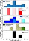 |
Fig. 3. Distribution of the 2–10 keV pulse fraction in percent for different source types. |
In polars, the spin and orbital periods are synchronized, ranging from 3000 s to 30 000 s (Scaringi et al. 2010). In our sample, the periods of polars vary from 4093 s to 6784 s, with the peak at ∼4800 s. The light curves of polars show constant modulation of depth with X-ray energies. The depths are generally higher compared to IPs (Norton & Watson 1989). In the middle panel of Fig. 3, it is evident that the pulse fraction for polars starts at higher values, around 30% compared to IPs, and that more polar type sources are found between 50% and 60%.
3.4. Spectral modeling
We performed time-averaged spectral modeling using the X-ray spectral fitting software XSPEC5 (Arnaud 1996). We employed χ2 statics in our model fitting. The spectra were fitted using a simple model composed of a power law and three Gaussian lines (tbabs(power-law+g1+g2+g3)). The Galactic absorption component is represented by tbabs (Wilms et al. 2000). For the continuum, we used a simple power-law model, and g1, g2, and g3 represent the three Gaussian lines at 6.4, 6.7, and 6.9 keV, respectively, for iron emission complex. While doing the fit, we freeze the line energies at the expected values, and the width of the lines is fixed at zero eV. We jointly fit the spectra of EPIC-pn, MOS1, and MOS2 detectors. While fitting the spectra, we included a constant factor for cross-calibration uncertainty, which is fixed to unity for EPIC-pn and allowed for variation for MOS1 and MOS2. The spectral fitting results are summarized in Table A.4, and Figs. A.3 and A.4 show the fitted spectra of the sources.
Figure 4 shows the distribution of absorption column density NH obtained from the X-ray spectral fitting. Overall, the NH distribution has a peak near 1022 cm−2, and more than 50% of the sources have NH between 1021 − 3.16 × 1022 cm−2. There are three sources with high NH > 1023 cm−2. The source 4XMM J175327.8–295716 has NH = 7 × 1020 cm−2, the lowest in our sample, which might indicate that this source is the closest to us among our sample or has a soft component that mimics the low NH.
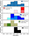 |
Fig. 4. Distribution of the absorption column density, NH, for different source types. |
Figure 5 shows the distribution of photon index Γ. The distribution has a peak at Γ ∼ 0.6. More than 50% of the sources have a flat spectral shape with Γ < 1. A significant number of sources in our sample have a softer spectrum with Γ > 1.2. We noticed that the majority of sources with high Γ values do not show any iron emission complex lines; only two of the seven sources with Γ ≥ 1.3, show strong emission lines in the 6–7 keV band.
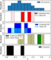 |
Fig. 5. Distribution of the photon index, Γ, for different source types. |
3.5. Gaia counterparts
A correct estimate of the distance to the source is required to derive their luminosity. For this, we searched for counterparts in the Gaia DR3 catalog. For each X-ray source, we computed the Gaia source density by counting the number of Gaia sources within a circle of 1′ radius at the source position. The Gaia density of sources is low and varies from 0.01–0.1 arcsec−2. We compute the probability of the sources having a spurious association by multiplying the Gaia source density with the area associated with the XMM-Newton positional error. Table 1 lists the sources for which we found a Gaia counterpart within the 3σ positional uncertainty of XMM-Newton. We found a likely Gaia counterpart for seven XMM-Newton sources. If a counterpart is found, then we use the Gaia source ID to find the distance to the source from Bailer-Jones et al. (2021). The distance to the sources for which a Gaia counterpart was found varies from ∼1.5 to ∼5 kpc and the X-ray luminosity is in the range 5 × 1032 − 6 × 1033 erg s−1.
Sources with possible Gaia optical counterparts.
4. Discussion
4.1. Typical properties of different classes of sources
We analyzed 444 XMM-Newton observations of the GC and the Galactic disk. We extracted X-ray light curves from nearly 2500 sources and systematically searched for X-ray pulsation. We detected periodicity in 26 sources, 14 of which are reported here for the first time. Many of the GC sources have a luminosity of a few times 1032 erg s−1 (Muno et al. 2003a), which is comparable to the luminosity typically observed in bright magnetic CVs (Verbunt et al. 1997; Ezuka & Ishida 1999). NS HMXRBs have much higher luminosity and are detected during their outburst period, reaching luminosities up to 1038 erg s−1. For the majority of the sources we did not find a Gaia counterpart due to the high absorption column density toward the GC and disk. Hence, the X-ray luminosity cannot be derived for a large number of sources and we cannot use this information to classify them. The NS HMXRBs are far less common in our Galaxy than the magnetic CVs. The nature of the Galactic sources is a long-standing question. Identifying the magnetic CVs or NS HMXRBs from X-ray periodicity alone can be difficult, as both types of sources usually display periods in a similar range. The short-period modulation in the X-ray light curve is thought to have originated from the spin period of the magnetically accreting WD or NS. In our sample, the smallest detected period is 1.36 s, and the maximum period detected is around 6784 s. The sample has a median period of 672 s. The pulse fraction of the modulation ranges from 10% to 80%. The detected periods are consistent with those of magnetic CVs and NSs in HMXRBs. A sample study of magnetic CVs indicates the median spin period is 6000 s (Ritter & Kolb 2003). There are also a few magnetic CVs with very short spin periods; for example, CTCV J2056–3014 has a spin period of 29.6 s (Lopes de Oliveira et al. 2020), and V1460 Her has a spin period of 38.9 s (Ashley et al. 2020). The spin periods of polars are mostly beyond 1 h, while almost all IPs have WD spin periods lower than 1 h. In contrast, 85 Galactic HMXRB pulsars (both with Be and OB supergiant companions) have a median (mean) spin period of 187 s (∼970 s), with only four sources showing a period longer than 1 h (Neumann et al. 2023).
It is evident that the different classes of sources (NS HMXRBs and magnetic CVs) exhibit a wide range of spin periods. Therefore, from the periodicity alone, it is difficult to understand the nature of the unclassified sources. Below we summarize a scheme to characterize the different classes of periodic X-ray sources utilizing their X-ray spectral, timing properties, and luminosity.
4.1.1. NS HMXRBs
The NS HMXRBs have properties that are very similar to IPs and they typically have very hard spectra. Figure 6 shows the period versus HR plot for classified and unclassified sources in our sample. The HR is calculated using the net counts in the 2–5 keV and 5–10 keV bands. We did not choose an energy band below 2 keV simply because it would be affected by Galactic absorption. The known NS HMXRBs appear very hard, similar to IPs; however, it is clear from Fig. 7 that they emit very little 6.7 keV iron line as compared to IPs. In almost all NS HMXRBs, the dominant component of the Fe K emission complex is the neutral 6.4 keV line emission and little to no ionized 6.7 and 6.9 keV line emission. This is because HMXRBs are mainly wind-fed systems, so the fluorescent iron line emission from the wind of the companion star is the main spectral feature in their spectra, while the ionized iron emission lines usually come from an accretion disk. The known NS HMXRBs in our sample – 4XMM J172511.3–361657 and 4XMM J174906.8–273233 – show no 6.7 keV emission, with upper limits on their equivalent widths (EWs) of 8 eV and 15 eV, respectively. We define the following criteria for the characterization of the NS HMXRB: (i) Pspin ≲ 1000 s, (ii) HR > −0.2, (iii)  eV, and (iv) a typical X-ray luminosity of 1033 − 1037 erg s−1.
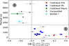 |
Fig. 6. HR vs. period diagram. The HR is calculated using the net counts of two bands: 2–5 keV and 5–10 keV. |
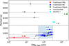 |
Fig. 7. EW of the 6.7 keV line vs. period diagram. |
4.1.2. IPs
One of the prominent features of IPs is the presence of strong ionized 6.7 keV line emission. In our sample, all the confirmed IPs have a clear detection of a 6.7 keV line, with the lowest EW of the sample being  for 4XMM J174517.0–321358. Xu et al. (2016) studied a sample of bright 17 IPs using Suzaku data. They found that the minimum and mean EW of the 6.7 keV line of the sample is
  and 107 ± 17 eV, respectively. The below criteria can be used to characterize IPs. They typically have (i) a spin period Pspin < 2500 s, (ii) an HR > −0.2, (iii) a strong 6.7 keV line emission with EW6.7 > 50 eV, and (iv) and an X-ray luminosity in the range 1031 − 1035 erg s−1 (Suleimanov et al. 2022).
4.1.3. Polars
The X-ray emission from polars is much softer than that of IPs. The spectra of many polars are dominated by very soft blackbody-like emission from the WD surface (Osborne et al. 1986; Ramsay et al. 1993; Clayton & Osborne 1994). However, toward the GC this component is difficult to observe due to the high absorption. In general polars also show a strong 6.7 keV line with an EW anywhere from 50 eV to ∼450 eV (Ezuka & Ishida 1999; Xu et al. 2016). As a whole, the detection of a 6.7 keV line in polar can be difficult for faint sources as they are much softer than IPs. Polars can be tentatively classified by having softer spectra and periods above 2500 s; however, a secure classification would require the detection of the 6.7 keV line with good quality X-ray spectra and strong circular polarization in the optical band. The polars can be characterized by the following characteristics: (i) Pspin = Porb > 2500 s, (ii) HR < −0.2, (iii) a strong 6.7 keV line emission with EW6.7 > 50 eV, and (iv) an X-ray luminosity below 1033 erg s−1 (Suleimanov et al. 2022).
4.2. Known NS HMXRBs
The source 4XMM J172511.3–361657 was discovered on 9 February 2004 by INTEGRAL and named as IGR J17252–3616 (Walter et al. 2004). XMM-Newton observed the source on 21 March 2004. A period search was performed by Zurita Heras et al. (2006), and a pulsation of 414.8 ± 0.5 s was discovered. An orbital period of 9.737 ± 0.004 days was also reported by using the Rossi X-ray Timing Explorer (RXTE) proportional counter array data (Markwardt & Swank 2003; Corbet et al. 2005). The source has a flat spectrum with  , which can also be fitted by a flat power law with an energy cutoff or a Comptonized model with kT ∼ 5.5 keV (Zurita Heras et al. 2006). The spectrum shows a 6.4 keV iron line with an EW of
  eV. Previous studies indicate the source is a wind-fed accreting pulsar with a supergiant companion star. The source has been observed multiple times by XMM-Newton, and we searched for pulsation in all the observations. The pulsations found in the different observations are consistent with each other within the 1σ error values. The source is highly variable, and the flux of the source can vary from 2.19 × 10⁻¹³ to 7.42 × 10⁻¹¹ erg s−1 cm−2. We noticed that whenever the source flux drops below ∼5 × 10⁻¹³ erg s−1 cm−2 the pulsation was undetectable.
The source 4XMM J174906.8–273233 was discovered in 1996 by ASCA. The source is also known as AXJ1749.1–2733 (Sakano et al. 2002). In a 1995 ASCA observation, the source was not detected, and in 2003 INTEGRAL caught a short outburst, which indicates its transient nature (Grebenev et al. 2004). XMM-Newton first observed 4XMM J174906.8–273233 on 31 March 2007, and Karasev et al. (2008) analyzed EPIC-pn data and detected a spin period of 132 s. The source was classified as a transient X-ray pulsar in a high-mass binary system. The source has been observed twice by XMM-Newton in 2007 and 2008; however, the pulsation was only detected in the 2007 observation (ObsID: 0510010401). The non-detection of pulsations in 2008 could be due to the combination of two factors: (1) the source flux was almost an order of magnitude fainter than in the 2007 observation, and (2) the 2008 observation had a shorter exposure than the 2007 observation, which led to ∼22 times fewer net counts in the 2008 observation than in the 2007 observation. The source spectrum is heavily absorbed and can be fitted by a steep power-law model with  ; adding an iron line at 6.4 keV improves the fit minutely.
4.3. Known IPs
The source 4XMM J174517.0–321358 (Gong 2022; Vermette et al. 2023) was discovered by Chandra and serendipitously observed by XMM-Newton in 2010. An iron-line emission complex and a pulsation of 614 s were detected using XMM-Newton data. The source is classified as an IP with a WD of 0.8 M⊙ (Vermette et al. 2023). The source has been observed twice by XMM-Newton, and in both observations, we detected a pulsation of 613 s. The X-ray spectrum looks like that of a typical IP with a flat spectral shape and iron emission complex.
The source 4XMM J174033.8–301501 was discovered by Suzaku in 2008 (Uchiyama et al. 2011a). Later, the source was observed by XMM-Newton on 18 March 2021 during a Galactic disk survey (Mondal et al. 2022). The source spectrum is well described by emission from collisionally ionized diffuse gas with a plasma temperature of ∼15.7 keV plus an iron line emission complex. A period of 432.4 s was detected in both Suzaku and XMM-Newton data. The source has been observed twice by XMM-Newton in 2018 and 2021. In both XMM-Newton observations, the detected pulsations are consistent. The source has a flat spectrum with  and an Fe emission complex in the 6–7 keV band.
4XMM J174954.6–294336 was first discovered by Chandra (Jonker et al. 2014). The source is classified as an IP based on the spin period of 1002 s and hard power-law spectral shape with complex iron line emission (Johnson et al. 2017; Mondal et al. 2023). This is only the second known IP that shows eclipses in X-rays. The source has been observed twice by XMM-Newton, and the pulsation is not visible in ObsID 0801681401. Mondal et al. (2023) discuss the possibility that the pulsation is suppressed due to a complex absorption behavior and the eclipse seen in the X-ray light curve.
4XMM J174917.7–283329 is classified as IP (Mondal et al. 2023). A period of 1212 s was detected in a 2017 XMM-Newton observation. The continuum is best fitted by a partially absorbed apec model with a plasma temperature of 13 keV. The source has been observed three times by XMM-Newton, but the pulsation was detected only once, when the source flux was one order of magnitude higher than in the other two observations.
The source 4XMM J174816.9–280750 was observed by BeppoSAX during the GC survey in 1997–1998 (Sidoli et al. 2006). The source has a spectrum with  and strong emission lines at 6–7 keV, plus a coherent pulsation of period 593 s was found in Suzaku and XMM-Newton data. These facts favor the source as an IP (Nobukawa et al. 2009). The source has been observed ten times by XMM-Newton, displaying significant variation in the pulsation period between different observations. A detailed, in-depth study of the source is required to determine whether the pulsation period variation is due to accretion or some other effects, such as the propeller phenomenon.
4XMM J174016.0–290337 was observed by XMM-Newton on 29 September 2005 (Farrell et al. 2010). The source displays Fe Kα emission and a periodic modulation with a period of 626 s. The source has been observed three times by XMM-Newton, and in all cases, a pulsation period of 622 s is detected.
The source 4XMM J174009.0–28472 was first discovered by ASCA (Sakano et al. 2000) and a period of 729 s was found. The source was classified as NS pulsar based on the flat power-law-type spectrum shape (Sakano et al. 2000). However, later near-infrared/optical studies suggested it is an IP (Kaur et al. 2010). The source has been observed four times by XMM-Newton, and we detected a similar pulsation period value in all observations. The source has a very flat spectrum  with strong emission lines.
4XMM J174622.7–285218 is classified as an IP (Nucita et al. 2022). The source was first observed in a Chandra observation of the GC, and a periodic signal of 1745 s was found (Muno et al. 2009). The spectrum is characterized by  , and the 6.9 keV line is the strongest with an EW of
  .
.
4.4. Known polars
The source 4XMM J174728.9–321441 was first observed by Chandra during the Galactic bulge survey (Jonker et al. 2014). The source is classified as a polar based on its long period of 4860 s detected in X-rays and in He IIλ5412 line emission (Wevers et al. 2017). This source has the steepest spectrum in our sample with  , and no iron emission complex was detected in the XMM-Newton spectrum. The non-detection of iron lines could be due to low signal-to-noise in the data.
4.5. Unclassified sources
Below, we try to classify the unknown sources using the scheme defined in Sect. 4.1. This is a tentative classification; further follow-up of the individual sources is required to constrain their true nature. For many sources, we do not have any Gaia counterpart; therefore, the estimation of the distance to the source using parallax was not possible and hence the luminosity is not calculated. In such a case, we only used the first three criteria for classification.
4.5.1. Likely NS HMXRBs
The only two sources matching the NS HMXRB criteria are XMMU J175441.9–265919 and 4XMM J175525.0–260402. Both have relatively high HR values: 0.02 ± 0.06 and 0.05 ± 0.02, respectively. The upper limits on the EWs of the 6.7 keV line for J175441.9 and J175525.0 are ∼28 eV and ∼34 eV, respectively. The spin periods of these two systems are 1.36 s and 392.5 s. The source J175525.0 was detected three times by XMM-Newton; however, the pulsation was detected only in the longest observation. A luminosity estimation was not possible as we did not find any counterparts in Gaia catalogs.
4.5.2. Likely IPs
The sources we categorize as IP are 4XMM J173058.9–350812, 4XMM J175301.3–291324, 4XMM J175740.5–285105, and 4XMM J175511.6–260315. The periods found from these systems are below 2500 s and the HRs are above −0.2. The 6.7 keV line EWs for the sources J173058.9, J175301.3, J175740.5, and J175511.6 are  , 105+189,
  , and
, and  eV, respectively. The source J175301.3 was observed three times by XMM-Newton, and a ∼672 s period was consistently found in two of those observations. The source J175511.6 was detected three times by XMM-Newton; however, the period of ∼1135 s was detected only in the longest observation. We detected a likely Gaia counterpart for the sources J173058.9 and J175511.6 and the distances estimated from their parallaxes are
  and
and  kpc, respectively. The luminosity of these two sources is in the range (0.8 − 1.9)×1033 erg s−1, which is typical for accreting magnetic CVs (Suleimanov et al. 2022).
4.5.3. Likely polars
The sources that are likely to be polars are 4XMM J173837.0–304818, 4XMM J175327.8–295716, 4XMM J175244.4–285851, 4XMM J175328.4–244627, and XMMU J180140.3–234221. These sources have very low HR values and long periods (see Fig. 6), which suggests that these sources are most likely to be polars. The long periods are most likely associated with the synchronized spin-orbital period of the WDs. All these sources have relatively soft spectra of photon index Γ = 0.8 − 2.1. For most of the polar-type sources, we have an upper limit on the EW of the 6.7 keV emission line. This is primarily because these sources have very low net counts that give ≤50 bins in the 0.2–10 keV spectrum. The source J175328.4 is the brightest in the polar sample and has the best signal-to-noise spectrum compared to the other four sources. In this case, the EW of the 6.7 keV emission line is  eV, which is much smaller than the typical values found in IPs. The source J175327.8 was observed six times by XMM-Newton; however, the periodicity was significantly detected only in the two observations that have an exposure above 25 ks. We found a likely Gaia counterpart for the source J175328.4 and its estimated distance is
  kpc, giving a luminosity of 2 × 1033 erg s−1.
4.5.4. Unknowns
We classify the sources XMMU J173029.8–330920, 4XMM J174809.8–300616, and 4XMM J175452.0–295758 as unknowns. These sources have high HR and periods similar to IPs. However, the 6.7 keV line was not detected clearly and we could only set an upper limit on its EW. The EW of the 6.7 keV line for the sources J173029.8, J174809.8, and J175452.0 are < 160, < 172, and < 206 eV, respectively. The source J174809.8 has been observed twice by XMM-Newton. However, it is relatively faint, with a flux of a few times 10−13 erg cm−2 s−1 and therefore the period was detected only in the longer observation. The source J175452.0 was detected three times by XMM-Newton; however, the pulsation was detected only in the longest observation.
4.5.5. NS or WD?
The compact object in 4XMM J174445.6–271344 is not clearly identified. Also known as HD 161103, it was observed by XMM-Newton on 26 January 2004. Lopes de Oliveira et al. (2006) did a detailed multiwavelength spectroscopic study of this source and suggested that the system hosts an NS; however, a WD scenario was not excluded. From optical spectroscopy, the companion star of this system is recognized as a Be star. We detected a periodicity of 3196 s from the X-ray light curve. The X-ray spectra show strong 6.4, 6.7, and 6.9 keV emission lines with EWs of  ,
,  , and
, and  eV, respectively. Such strong 6.7 and 6.9 keV emission lines are not typically seen in accreting NS HMXRBs. Also, the source has a much softer spectrum (HR = − 0.42 ± 0.03 in Fig. 6) than the two confirmed NS HMXRBs (4XMM J172511.3–361657 and 4XMM J172511.3–361657) in our sample.
5. Conclusion
We systematically searched for periodic X-ray sources in the inner Galactic disk, which extends from l ∼ 350° to l ∼ +7° and includes the GC, using XMM-Newton Heritage observations and archival data. We find 26 sources that show periodicity in their X-ray light curves, of which 12 have previously reported periods. For these 12 sources, we have obtained periods consistent with those previously reported. We have detected the periodicity in the other 14 sources for the first time. We classified the sources based on the values of the HR, period, and iron emission complex in the 6–7 keV band. Of these 14 sources, we classify two as NS X-ray binaries, four as likely IPs, five as likely polars, and three as unknowns. The IP-type sources display a steep X-ray spectrum with Γ ≤ 1.1 and an iron emission complex in the 6–7 keV band. The spectra of polars are much softer compared to IPs.
We also detected a few sources with detection significance of the pulsation just above the 1σ confidence level. We did not list these sources in Table A.1; one such example is the transient Galactic bulge IP XMMU J175035.2–293557 (Hofmann et al. 2018).
Acknowledgments
SM and GP acknowledge financial support from the European Research Council (ERC) under the European Union’s Horizon 2020 research and innovation program HotMilk (grant agreement No. 865637). SM and GP also acknowledge support from Bando per il Finanziamento della Ricerca Fondamentale 2022 dell’Istituto Nazionale di Astrofisica (INAF): GO Large program and from the Framework per l’Attrazione e il Rafforzamento delle Eccellenze (FARE) per la ricerca in Italia (R20L5S39T9). KM is partially supported by the NASA ADAP program (NNH22ZDA001N-ADAP). We thank the referee for the comments, corrections, and suggestions that significantly improved the manuscript.
References
- Aizu, K. 1973, Prog. Theor. Phys., 49, 1184 [CrossRef] [Google Scholar]
- Anastasopoulou, K., Ponti, G., Sormani, M. C., et al. 2023, A&A, 671, A55 [NASA ADS] [CrossRef] [EDP Sciences] [Google Scholar]
- Arnaud, K. A. 1996, in Astronomical Data Analysis Software and Systems V, eds. G. H. Jacoby, & J. Barnes, ASP Conf. Ser., 101, 17 [NASA ADS] [Google Scholar]
- Ashley, R. P., Marsh, T. R., Breedt, E., et al. 2020, MNRAS, 499, 149 [NASA ADS] [CrossRef] [Google Scholar]
- Astropy Collaboration (Robitaille, T. P. et al.) 2013, A&A, 558, A33 [NASA ADS] [CrossRef] [EDP Sciences] [Google Scholar]
- Astropy Collaboration (Price-Whelan, A. M. et al.) 2018, AJ, 156, 123 [Google Scholar]
- Astropy Collaboration (Price-Whelan, A. M. et al.) 2022, ApJ, 935, 167 [NASA ADS] [CrossRef] [Google Scholar]
- Bahramian, A., Heinke, C. O., Kennea, J. A., et al. 2021, MNRAS, 501, 2790 [NASA ADS] [CrossRef] [Google Scholar]
- Bailer-Jones, C. A. L., Rybizki, J., Fouesneau, M., Demleitner, M., & Andrae, R. 2021, AJ, 161, 147 [Google Scholar]
- Baluev, R. V. 2008, MNRAS, 385, 1279 [Google Scholar]
- Bao, T., & Li, Z. 2022, MNRAS, 509, 3504 [Google Scholar]
- Clayton, K. L., & Osborne, J. P. 1994, MNRAS, 268, 229 [NASA ADS] [CrossRef] [Google Scholar]
- Corbet, R. H. D., Markwardt, C. B., & Swank, J. H. 2005, ApJ, 633, 377 [NASA ADS] [CrossRef] [Google Scholar]
- Cropper, M. 1990, Space Sci. Rev., 54, 195 [CrossRef] [Google Scholar]
- Downes, R. A., Webbink, R. F., Shara, M. M., et al. 2001, PASP, 113, 764 [Google Scholar]
- Ezuka, H., & Ishida, M. 1999, ApJS, 120, 277 [NASA ADS] [CrossRef] [Google Scholar]
- Farrell, S. A., Gosling, A. J., Webb, N. A., et al. 2010, A&A, 523, A50 [NASA ADS] [CrossRef] [EDP Sciences] [Google Scholar]
- Foreman-Mackey, D., Hogg, D. W., Lang, D., & Goodman, J. 2013, PASP, 125, 306 [Google Scholar]
- Gong, H. 2022, ApJ, 933, 240 [NASA ADS] [CrossRef] [Google Scholar]
- Grebenev, S. A., Rodriguez, J., Westergaard, N. J., Sunyaev, R. A., & Oosterbroek, T. 2004, ATel, 252, 1 [NASA ADS] [Google Scholar]
- Haberl, F., & Motch, C. 1995, A&A, 297, L37 [NASA ADS] [Google Scholar]
- Hailey, C. J., Mori, K., Perez, K., et al. 2016, ApJ, 826, 160 [NASA ADS] [CrossRef] [Google Scholar]
- Hofmann, F., Ponti, G., Haberl, F., & Clavel, M. 2018, A&A, 615, L7 [NASA ADS] [CrossRef] [EDP Sciences] [Google Scholar]
- Jansen, F., Lumb, D., Altieri, B., et al. 2001, A&A, 365, L1 [NASA ADS] [CrossRef] [EDP Sciences] [Google Scholar]
- Johnson, C. B., Torres, M. A. P., Hynes, R. I., et al. 2017, MNRAS, 466, 129 [NASA ADS] [CrossRef] [Google Scholar]
- Jonker, P. G., Torres, M. A. P., Hynes, R. I., et al. 2014, ApJS, 210, 18 [NASA ADS] [CrossRef] [Google Scholar]
- Karasev, D. I., Tsygankov, S. S., & Lutovinov, A. A. 2008, MNRAS, 386, L10 [NASA ADS] [CrossRef] [Google Scholar]
- Kaur, R., Wijnands, R., Paul, B., Patruno, A., & Degenaar, N. 2010, MNRAS, 402, 2388 [NASA ADS] [CrossRef] [Google Scholar]
- Lomb, N. R. 1976, Ap&SS, 39, 447 [Google Scholar]
- Lopes de Oliveira, R., Motch, C., Haberl, F., Negueruela, I., & Janot-Pacheco, E. 2006, A&A, 454, 265 [NASA ADS] [CrossRef] [EDP Sciences] [Google Scholar]
- Lopes de Oliveira, R., Bruch, A., Rodrigues, C. V., Oliveira, A. S., & Mukai, K. 2020, ApJ, 898, L40 [NASA ADS] [CrossRef] [Google Scholar]
- Markwardt, C. B., & Swank, J. H. 2003, ATel, 179, 1 [NASA ADS] [Google Scholar]
- Mondal, S., Ponti, G., Haberl, F., et al. 2022, A&A, 666, A150 [NASA ADS] [CrossRef] [EDP Sciences] [Google Scholar]
- Mondal, S., Ponti, G., Haberl, F., et al. 2023, A&A, 671, A120 [NASA ADS] [CrossRef] [EDP Sciences] [Google Scholar]
- Mukai, K. 2017, PASP, 129, 062001 [Google Scholar]
- Muno, M. P., Baganoff, F. K., Bautz, M. W., et al. 2003a, ApJ, 589, 225 [NASA ADS] [CrossRef] [Google Scholar]
- Muno, M. P., Baganoff, F. K., Bautz, M. W., et al. 2003b, ApJ, 599, 465 [NASA ADS] [CrossRef] [Google Scholar]
- Muno, M. P., Arabadjis, J. S., Baganoff, F. K., et al. 2004, ApJ, 613, 1179 [Google Scholar]
- Muno, M. P., Bauer, F. E., Baganoff, F. K., et al. 2009, ApJS, 181, 110 [CrossRef] [Google Scholar]
- Neumann, M., Avakyan, A., Doroshenko, V., & Santangelo, A. 2023, A&A, 677, A134 [NASA ADS] [CrossRef] [EDP Sciences] [Google Scholar]
- Nishiyama, S., Yasui, K., Nagata, T., et al. 2013, ApJ, 769, L28 [Google Scholar]
- Nobukawa, M., Koyama, K., Matsumoto, H., & Tsuru, T. G. 2009, PASJ, 61, S93 [CrossRef] [Google Scholar]
- Norton, A. J., & Watson, M. G. 1989, MNRAS, 237, 853 [Google Scholar]
- Nucita, A. A., Lezzi, S. M., De Paolis, F., et al. 2022, MNRAS, 517, 118 [NASA ADS] [CrossRef] [Google Scholar]
- Osborne, J. P., Bonnet-Bidaud, J. M., Bowyer, S., et al. 1986, MNRAS, 221, 823 [NASA ADS] [CrossRef] [Google Scholar]
- Patterson, J. 1994, PASP, 106, 209 [Google Scholar]
- Perez, K., Hailey, C. J., Bauer, F. E., et al. 2015, Nature, 520, 646 [NASA ADS] [CrossRef] [Google Scholar]
- Ponti, G., Morris, M. R., Terrier, R., & Goldwurm, A. 2013, in Cosmic Rays in Star-Forming Environments, eds. D. F. Torres, & O. Reimer, Astrophys. Space Sci. Proc., 34, 331 [NASA ADS] [CrossRef] [Google Scholar]
- Ponti, G., Morris, M. R., Terrier, R., et al. 2015, MNRAS, 453, 172 [Google Scholar]
- Ponti, G., Hofmann, F., Churazov, E., et al. 2019, Nature, 567, 347 [Google Scholar]
- Ponti, G., Morris, M. R., Churazov, E., Heywood, I., & Fender, R. P. 2021, A&A, 646, A66 [NASA ADS] [CrossRef] [EDP Sciences] [Google Scholar]
- Predehl, P., Sunyaev, R. A., Becker, W., et al. 2020, Nature, 588, 227 [CrossRef] [Google Scholar]
- Ramsay, G., Rosen, S. R., Mason, K. O., Cropper, M. S., & Watson, M. G. 1993, MNRAS, 262, 993 [NASA ADS] [CrossRef] [Google Scholar]
- Revnivtsev, M., Sazonov, S., Churazov, E., et al. 2009, Nature, 458, 1142 [Google Scholar]
- Ritter, H., & Kolb, U. 2003, A&A, 404, 301 [NASA ADS] [CrossRef] [EDP Sciences] [Google Scholar]
- Sakano, M., Torii, K., Koyama, K., Maeda, Y., & Yamauchi, S. 2000, PASJ, 52, 1141 [NASA ADS] [CrossRef] [Google Scholar]
- Sakano, M., Koyama, K., Murakami, H., Maeda, Y., & Yamauchi, S. 2002, ApJS, 138, 19 [NASA ADS] [CrossRef] [Google Scholar]
- Saxton, C. J., Wu, K., Cropper, M., & Ramsay, G. 2005, MNRAS, 360, 1091 [NASA ADS] [CrossRef] [Google Scholar]
- Scargle, J. D. 1982, ApJ, 263, 835 [Google Scholar]
- Scaringi, S., Bird, A. J., Norton, A. J., et al. 2010, MNRAS, 401, 2207 [NASA ADS] [CrossRef] [Google Scholar]
- Sidoli, L., Mereghetti, S., Favata, F., Oosterbroek, T., & Parmar, A. N. 2006, A&A, 456, 287 [NASA ADS] [CrossRef] [EDP Sciences] [Google Scholar]
- Strüder, L., Briel, U., Dennerl, K., et al. 2001, A&A, 365, L18 [Google Scholar]
- Su, M., Slatyer, T. R., & Finkbeiner, D. P. 2010, ApJ, 724, 1044 [Google Scholar]
- Suleimanov, V. F., Doroshenko, V., & Werner, K. 2022, MNRAS, 511, 4937 [NASA ADS] [CrossRef] [Google Scholar]
- Timmer, J., & Koenig, M. 1995, A&A, 300, 707 [NASA ADS] [Google Scholar]
- Turner, M. J. L., Abbey, A., Arnaud, M., et al. 2001, A&A, 365, L27 [CrossRef] [EDP Sciences] [Google Scholar]
- Uchiyama, H., Koyama, K., Matsumoto, H., et al. 2011a, PASJ, 63, S865 [NASA ADS] [CrossRef] [Google Scholar]
- Uchiyama, H., Nobukawa, M., Tsuru, T., Koyama, K., & Matsumoto, H. 2011b, PASJ, 63, S903 [NASA ADS] [CrossRef] [Google Scholar]
- Vaughan, S. 2010, MNRAS, 402, 307 [NASA ADS] [CrossRef] [Google Scholar]
- Vaughan, S., Edelson, R., Warwick, R. S., & Uttley, P. 2003, MNRAS, 345, 1271 [Google Scholar]
- Verbunt, F., Bunk, W. H., Ritter, H., & Pfeffermann, E. 1997, A&A, 327, 602 [NASA ADS] [Google Scholar]
- Vermette, B., Salcedo, C., Mori, K., et al. 2023, ApJ, 954, 138 [NASA ADS] [CrossRef] [Google Scholar]
- Walter, R., Bodaghee, A., Barlow, E. J., et al. 2004, ATel, 229, 1 [NASA ADS] [Google Scholar]
- Wang, Q. D., Gotthelf, E. V., & Lang, C. C. 2002, Nature, 415, 148 [NASA ADS] [CrossRef] [Google Scholar]
- Warner, B. 1989, Inf. Bull. Var. Stars, 3383, 1 [NASA ADS] [Google Scholar]
- Warner, B. 2003, Cataclysmic Variable Stars (Cambridge, UK: Cambridge University Press) [Google Scholar]
- Warwick, R. S., Turner, M. J. L., Watson, M. G., & Willingale, R. 1985, Nature, 317, 218 [NASA ADS] [CrossRef] [Google Scholar]
- Webb, N. A., Coriat, M., Traulsen, I., et al. 2020, A&A, 641, A136 [NASA ADS] [CrossRef] [EDP Sciences] [Google Scholar]
- Wevers, T., Torres, M. A. P., Jonker, P. G., et al. 2017, MNRAS, 470, 4512 [NASA ADS] [CrossRef] [Google Scholar]
- Wilms, J., Allen, A., & McCray, R. 2000, ApJ, 542, 914 [Google Scholar]
- Worrall, D. M., Marshall, F. E., Boldt, E. A., & Swank, J. H. 1982, ApJ, 255, 111 [Google Scholar]
- Xu, X.-J., Wang, Q. D., & Li, X.-D. 2016, ApJ, 818, 136 [NASA ADS] [CrossRef] [Google Scholar]
- Yamauchi, S., Kaneda, H., Koyama, K., et al. 1996, PASJ, 48, L15 [NASA ADS] [Google Scholar]
- Yasui, K., Nishiyama, S., Yoshikawa, T., et al. 2015, PASJ, 67, 123 [NASA ADS] [CrossRef] [Google Scholar]
- Zhu, Z., Li, Z., & Morris, M. R. 2018, ApJS, 235, 26 [NASA ADS] [CrossRef] [Google Scholar]
- Zurita Heras, J. A., De Cesare, G., Walter, R., et al. 2006, A&A, 448, 261 [NASA ADS] [CrossRef] [EDP Sciences] [Google Scholar]
Appendix A: Additional figures and tables
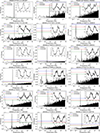 |
Fig. A.1. Lomb-Scargle periodogram of the sources listed in Table A.1. The periodograms are constructed using 2–10 keV EPIC-pn light curves. The horizontal green and red lines indicate the 2σ and 3σ confidence levels, respectively, computed from simulations, and the blue line indicates the false alarm probability (3σ confidence level) estimated from the analytical approximation from Baluev (2008). The small inset shows the folded light curve. |
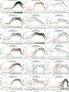 |
Fig. A.3. Spectral modeling of the sources in our sample using a model composed of tbabs*(power-law+g1+g2+g3). The g1,g2, and g3 represent three Gaussian lines, at 6.4, 6.7, and 6.9 keV, respectively. The black, red, and green colors represent data from the EPIC-pn, MOS1, and MOS2 detectors, respectively. |
Various details of the X-ray pulsators in the GC plus Galactic disk.
Details of the pulsators for which more than one observation is available.
Table A.2 Continued.
Details of the spectral fit.
All Tables
All Figures
|
Fig. 1. Mosaic of the exposure maps created using the ongoing XMM-Newton observations of the Galactic disk plus archival observations of the GC. The small red, blue, and green circles show the positions of confirmed or likely NSs, IPs, and polars, respectively. The black circles indicate the unclassified sources. |
| In the text | |
|
Fig. 2. Distribution of log(period) for various source types. |
| In the text | |
|
Fig. 3. Distribution of the 2–10 keV pulse fraction in percent for different source types. |
| In the text | |
|
Fig. 4. Distribution of the absorption column density, NH, for different source types. |
| In the text | |
|
Fig. 5. Distribution of the photon index, Γ, for different source types. |
| In the text | |
|
Fig. 6. HR vs. period diagram. The HR is calculated using the net counts of two bands: 2–5 keV and 5–10 keV. |
| In the text | |
|
Fig. 7. EW of the 6.7 keV line vs. period diagram. |
| In the text | |
|
Fig. A.1. Lomb-Scargle periodogram of the sources listed in Table A.1. The periodograms are constructed using 2–10 keV EPIC-pn light curves. The horizontal green and red lines indicate the 2σ and 3σ confidence levels, respectively, computed from simulations, and the blue line indicates the false alarm probability (3σ confidence level) estimated from the analytical approximation from Baluev (2008). The small inset shows the folded light curve. |
| In the text | |
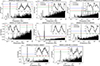 |
Fig. A.2. Fig. A.1 Continued. |
| In the text | |
|
Fig. A.3. Spectral modeling of the sources in our sample using a model composed of tbabs*(power-law+g1+g2+g3). The g1,g2, and g3 represent three Gaussian lines, at 6.4, 6.7, and 6.9 keV, respectively. The black, red, and green colors represent data from the EPIC-pn, MOS1, and MOS2 detectors, respectively. |
| In the text | |
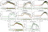 |
Fig. A.4. Fig. A.3 Continued. |
| In the text | |
Current usage metrics show cumulative count of Article Views (full-text article views including HTML views, PDF and ePub downloads, according to the available data) and Abstracts Views on Vision4Press platform.
Data correspond to usage on the plateform after 2015. The current usage metrics is available 48-96 hours after online publication and is updated daily on week days.
Initial download of the metrics may take a while.