| Issue |
A&A
Volume 698, June 2025
|
|
|---|---|---|
| Article Number | A206 | |
| Number of page(s) | 12 | |
| Section | Galactic structure, stellar clusters and populations | |
| DOI | https://doi.org/10.1051/0004-6361/202553664 | |
| Published online | 17 June 2025 | |
A sample of ionised Fe line-emitting X-ray sources in the inner Galactic disc
1
INAF – Osservatorio Astronomico di Brera,
Via E. Bianchi 46,
23807
Merate (LC),
Italy
2
Department of Astronomy, University of Illinois,
1002 W. Green St.,
Urbana,
IL
61801,
USA
3
Max-Planck-Institut für extraterrestrische Physik,
Gießenbachstraße 1,
85748
Garching,
Germany
4
Department of Physics and Astronomy, University of California,
Los Angeles,
CA
90095-1547,
USA
5
Institute of Space Sciences (ICE, CSIC),
Campus UAB, Carrer de Can Magrans s/n,
08193
Barcelona,
Spain
6
Institut d'Estudis Espacials de Catalunya (IEEC),
Carrer Gran Capità 2–4,
08034
Barcelona,
Spain
★ Corresponding author: samaresh.astro@gmail.com
Received:
2
January
2025
Accepted:
25
April
2025
Context. The origin of the unresolved X-ray emission towards the Galactic Centre and the Galactic disc is unclear. Previous studies suggest that the Galactic diffuse X-ray emission is composed of unresolved point sources, primarily magnetic cataclysmic variables (mCVs). However, mCVs have a much lower 6.7 keV line equivalent width (EW6.7) and a much higher line intensity ratio between Fe XXVI and Fe XXV (I6.9/I6.7) compared to the diffuse X-ray emission. Therefore, the primary contributors to the unresolved X-ray emission remain unclear.
Aims. We performed a deep X-ray scan of the inner Galactic disc using XMM-Newton observations covering 350° < l < 7° and -0.8° < b < +0.8°. We aim to characterise the different populations of point sources that contribute to the Galactic diffuse X-ray emission by estimating the X-ray spectral slope Γ in the 0.2–10 keV band, EW6.7, and I6.9/I6.7.
Methods. We performed source detection in the 6.5–7 keV band. We then extracted the spectra of the X-ray point sources and performed spectral modelling using XSPEC to estimate the X-ray spectral index Γ, equivalent width, and intensities of the iron 6.7 and 6.9 keV lines.
Results. We detected a total of 859 sources in the 6.5–7 keV band, of which 72 sources show significant iron line emission at 6.7 keV. The distribution of spectral index Γ for these 72 sources is bimodal, with peaks at Γ = 0.5 ± 0.4 and 1.8 ± 0.3, suggesting two populations of sources. The soft X-ray sources (Γ ∼ 1.8) have significantly larger EW6.7 than the hard X-ray sources (Γ ∼ 0.5). Furthermore, 18 of the 32 hard sources are associated with previously known CVs. We identify CV candidates in our sample as those with spectral index Γ < 1.25. The line ratio, 2–10 keV luminosity, and previous detection of spin period suggest that most of these CVs are magnetic. The distribution of the EW6.7 line for the combined sample of previously identified and candidate CVs has a mean value of ⟨EW6.7⟩ = 415 ± 39 eV. Furthermore, we computed the stacked spectra of all sources detected in the 6.5–7 keV band for different flux groups, and we find evidence in the stacked spectra of hard sources that the EW6.7 increases with decreasing flux. The soft X-ray sources have ⟨EW6.7⟩ = 1.1 ± 0.1 keV. We identified 13 of the 30 soft sources associated with active stars, young stellar objects, and active binaries of RS CVn type.
Conclusions. The Fe XXV line-emitting sources towards the Galactic disc can be broadly categorised into two types: soft and hard X-ray sources. The ⟨EW6.7⟩ of our CV candidate sample is more than twice as large as the typical EW6.7 found in mCVs within 500 pc, and the ⟨EW6.7⟩ of our CV candidate sample is close to the EW6.7 value of Galactic diffuse X-ray emission. In our survey, the detection sensitivity for point sources in the 6.5–7 keV band is ∼10−14 erg s−1 cm−2. Therefore, up to a flux limit of ∼10−14 erg s−1 cm−2 or higher, nearly 50% of Galactic diffuse X-ray emission in the 6.5–7 keV band originates from mCVs. The large ⟨EW6.7⟩ of the soft source sample indicates that these sources also contribute significantly to the Galactic diffuse X-ray emission, as well as from CVs.
Key words: novae, cataclysmic variables / white dwarfs / Galaxy: bulge / Galaxy: center / Galaxy: disk / X-rays: binaries
© The Authors 2025
 Open Access article, published by EDP Sciences, under the terms of the Creative Commons Attribution License (https://creativecommons.org/licenses/by/4.0), which permits unrestricted use, distribution, and reproduction in any medium, provided the original work is properly cited.
This article is published in open access under the Subscribe to Open model. Subscribe to A&A to support open access publication.
1 Introduction
Early X-ray observations have revealed a large-scale, diffuse X- ray emission of Galactic origin (see Ponti et al. 2013, for a review of X-ray activity in the Galactic Centre). The Galactic diffuse X- ray emission has a surface brightness slightly higher than that of the cosmic X-ray background, but it is more concentrated along the Galactic plane, with a scale height of only a few hundred parsecs (Yamauchi et al. 2016). This emission can be decomposed into three spatial components: Galactic centre X-ray emission (GCXE; Kellogg et al. 1971; Watson et al. 1981), Galactic bulge X-ray emission (GBXE; Cooke et al. 1969; Warwick et al. 1980), and Galactic ridge X-ray emission (GRXE; Worrall et al. 1982; Warwick et al. 1985). The Galactic diffuse X-ray emission shows multiple iron emission lines, with the K-shell transition line from He-like Fe (Fe XXV-Heα) at 6.7 keV being the brightest. The 6.7 keV iron line emission is a significant feature in X-ray astronomy, particularly in the context of our Galaxy (Koyama 2018). This emission is primarily associated with ionised iron and provides critical insights into the physical conditions and processes occurring in the Galactic environment. Uchiyama et al. (2013) performed a survey with Suzaku of the Galactic Centre (GC) region and additional regions at higher longitude l and higher latitude b, demonstrating that the intensity of the Fe XXV line increases towards the GC. The overall Galactic diffuse X-ray emission spectrum can be fitted by a two-temperature, collisionally ionised plasma model with temperatures of -0.75 and ∼7.5 keV (Nobukawa et al. 2016).
The 6.7 keV line emission serves as a diagnostic tool for studying hot plasma environments, which are indicative of energetic processes such as supernova remnants and active stellar populations (Porquet et al. 2010). Initially, the Galactic diffuse X-ray emission was interpreted as hot plasma confined within the Galactic potential well (Watson et al. 1981; Warwick et al. 1985). However, the Galactic potential well is too shallow to confine such a hot plasma (Tanaka 2002; Belmont et al. 2005). The correlation between the 6.7 keV line intensity of Galactic diffuse X-ray emission and the near-infrared surface brightness across different regions supports a link to star formation and stellar activity (Revnivtsev et al. 2006). A recent study by Anastasopoulou et al. (2023) showed that the diffuse hard emission in the central degrees at the GC can be explained by assuming a GC stellar population with iron abundances -1.9 times higher than those in the Galactic bar or bulge. In some regions of the Galactic diffuse X-ray emission, Chandra has resolved 80% of the 6.7 keV emission as X-ray point sources (Revnivtsev et al. 2009). The hotter -7.5 keV emission of the Galactic diffuse X-ray emission is thought to originate from unresolved, accreting magnetic cataclysmic variables (mCVs). A similar study by Hong (2012) suggested that, above 3 keV, 80% of the resolved sources are mCVs, while the net emission from active binaries (ABs) constitutes the remaining 20%. A recent study by Koyama & Nobukawa (2024) attempted to fit the spectra of the GCXE, GRXE, and GBXE with the composite spectra of all local white dwarfs (WD) and X-ray active stars, suggesting that additional components are still required, which may indicate the presence of truly diffuse emission originating from supernova remnants.
The emission from mCVs, including intermediate polars (IPs) and polars, is dominated by hard X-ray emission and ionised lines between 6.5–7.0 keV. In mCVs, accretion shocks above the WD surface heat the infalling material, leading to temperatures of kT > 15 keV. These extremely high temperatures ionise the medium, which emits the Fe XXV and Fe XXVI lines at 6.7 and 6.9 keV, respectively. In addition, mCVs exhibit fluorescent Fe Kα line emission at 6.4 keV, originating from the reflection of X-rays off the WD surface (see Cropper 1990; Patterson 1994; Mukai 2017, for a review on accreting WD binaries). Ezuka & Ishida (1999) studied a sample of 20 magnetic CVs and found average equivalent widths (EWs) of EW6.4 ∼ 100, EW6.7 ∼ 170, and EW6.9 ∼ 100 eV, for the 6.4, 6.7, and 6.9 keV lines, respectively. Similar EW values were reported by Hellier et al. (1998). Furthermore, Hellier & Mukai (2004) investigated a sample of five mCVs using Chandra high energy transmission grating spectra and found average EW values of EW6.4 ∼ 120, EW6.7 ∼ 160, and EW6.9 ∼ 110 eV. More recently, Xu et al. (2016) studied a sample of 20 mCVs and found mean EW6.7 values of 107 ± 16 eV for IPs and 221 ± 135 for polars. Previous studies have highlighted that the EWs of the 6.4 and 6.9 keV iron lines in the mCV population are similar to those in the Galactic diffuse X-ray emission. However, their EW6.7 values are 2-3 times smaller than in the GCDE or GRXE.
The line intensity ratio between Fe XXVI and Fe XXV ( ) in the mCV population also differs significantly from the Galactic diffuse X-ray emission. For example, the GCXE and GRXE have EW6.7 values of 500 ± 3 and 487 ± 13 eV, respectively (Nobukawa et al. 2016). The line intensity ratio
  for the GCXE and GRXE is 0.367 ± 0.005 and 0.16 ± 0.02, respectively (Koyama 2018). In contrast, the mean EW6.7 of the mCV population in the solar neighbourhood is ∼ 160 eV (Ezuka & Ishida 1999; Hellier et al. 1998; Xu et al. 2016), and the intensity ratio
  of mCVs in the solar neighbourhood varies between 0.4–0.7 (Xu et al. 2016). For the active binary (AB) population, both the EW6.7 and the values are significantly lower than those of the GCXE and GRXE. The AB population typically has an EW6.7 of ∼327 eV and a line intensity ratio of ∼0.14 (Nobukawa et al. 2016). As the EW6.7 and
  values of mCV and AB populations do not match those of the GCXE and GRXE, it remains unclear how the GCXE and GRXE decompose into specific X-ray source classes and what their contributions are to the total emission component. In this study, we use the EW6.7 of the ionised Fe XXV line and the line intensity ratio as diagnostic tools to probe the temperature and metallicity of the X-ray emitting plasma, and to constrain the nature and population of the underlying source classes responsible.
2 Data reduction
We conducted an X-ray scan (PI: G. Ponti) of the inner Galactic disc covering 350° < l < 7° and -0.8° < b < +0.8°. Details of the Heritage survey, including the multi-band X-ray mosaic of the region, will be presented in a forthcoming paper (Ponti et al., in prep.). We analysed a total of 588 XMM-Newton (Jansen et al. 2001) observations, including the Heritage data for the inner Galactic disc and archival observations of the Galactic Centre (Ponti et al. 2015, 2019). The observation data files were processed using the XMM-Newton Science Analysis System (SASv19.0.0)1. This work is largely based on the XMM-Newton data set presented in Mondal et al. (2024a), with slightly different selection criteria, as described below. High background flaring activity was filtered out after careful inspection. We removed the time interval of increased flaring activity when the background was above a threshold of 8 counts ks−1 arcmin−2 for EPIC-pn (Strüder et al. 2001) and 2.5 counts ks−1 arcmin−2 for EPIC-MOS1/MOS2 (Turner et al. 2001) in the 715 keV bands. We used the SAS task emldetect to detect point sources and generate the source list. Detection was performed in five energy bands: 1–4.5, 4.5–6, 6–6.5, 6.5–7, and 7–12 keV. We computed the maximum likelihood (ML) and net counts in the broadband 1–12 keV band from the sub-bands. We chose EXT==0 to select only the point sources. We also applied an ML cut to detect sources that were more likely to be real. Therefore, to construct the cleanest sample, we chose ML > 14, where all sources are statistically real with a > 5σ confidence level (Webb et al. 2020). We detected a total of 859 sources with ML > 14 in the 6.5–7 keV band. We extracted the spectra using the SAS task evselect. We selected events with PATTERN≤4 and PATTERNS≤12 for EPIC-pn and MOS1/MOS2 detectors, respectively. We chose a circular region of 20" radius for the source product extraction. The background products were extracted from an annular region centred on the source position, with inner and outer radii of 25" and 30", respectively. The spectra from each detector (pn, MOS1, or MOS2) were grouped to have a signal-to-noise ratio (S/N) of 3 in each energy bin.
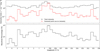 |
Fig. 1 Top panel: longitude profile of total emission (point sources plus unresolved emission) in the 6.5–7.0 keV range, integrated over -0.8° ≤ b ≤ 0.8° (black curve). The red curve shows the contribution from point sources detected with ML > 14 in the 1–12 keV band. Bottom panel: percentage of the total 6.5–7.0 keV emission resolved by X-ray point sources. |
3 Spectral fitting procedure
We utilised PyXspec, a Python interface to XSPEC for automated X-ray spectral fitting (Arnaud 1996; Gordon & Arnaud 2021). We used 𝒳2 statistics in our spectral modelling and estimated the 95% error for each fitting parameter. Before estimating the iron line EW, it is essential to select the correct continuum model that properly fits the 0.2–10 keV X-ray spectra. The choice of the X-ray continuum model is crucial in estimating the significance and EW of the detected line. We tested two continuum models: a power-law model and a blackbody plus power-law model. If the continuum model does not adequately describe the data, the estimation of line intensity and EW can be significantly biased. In sources whose emission is dominated by soft photons, their continuum might not be well described by a simple absorbed power-law model, potentially leading to errors in EW estimation. Therefore, for each source, we compared the fit quality of the simple power-law and blackbody plus power-law models by examining their 𝒳2 and degrees of freedom (d.o.f.). We favoured the blackbody plus power-law continuum model over the simple power-law model if it improved the continuum fitting above the 3a confidence level. During the fit, we included an absorption component tbabs with the default abundance value wilm (Wilms et al. 2000) to account for the absorption of X-rays along the line of sight by the interstellar medium.
For each source, we first fitted the spectrum with the selected continuum model and recorded the fit parameters, 𝒳2 and d.o.f. values. We then added a Gaussian component at 6.7 keV and computed the fit statistics. We fixed the centroid of the line at 6.7 keV and the line width at zero eV while performing the fit. The XMM-Newton spectral resolution cannot resolve the thermal broadening of the line; therefore, we fixed the width of the line at zero eV. We evaluated the improvement in fit by calculating Δ𝒳2 and computed the statistical significance of the line using an F test. Next, we computed the EW and the intensity of the line. We repeated this procedure for the Fe XXVI line by adding a Gaussian at 6.9 keV and similarly computed the EW, line intensity, and significance of the line.
4 Results
4.1 Emission profile and resolved percentage
We compared the total X-ray emission in the 6.5–7 keV band with the emission from resolved point sources. To compute the emission profile, we selected a strip of -0.8° ≤ b ≤ +0.8° and longitude l that extended from 350° to 7°. We constructed a count-rate mosaic map from all XMM-Newton observations considered in this study, which was subsequently smoothed using a Gaussian kernel of σ = 5 pixels; each pixel has a size of 4 × 4 arcsec2. We computed the intensity profile considering a sliding box with a longitude bin size ∆l = 0.5° and b = ±0.8°. We then calculated the total intensity of a given sky area in the 6.5–7 keV band (resolved point sources plus unresolved emission). Furthermore, we also computed the intensity of the 6.5–7 keV emission from point sources only. The top panel of Fig. 1 shows the longitudinal profile of the total emission intensity (black curve). The red curve shows the intensity of the X-ray emission from point sources only. During the calculation of the intensity profile, the count rate was averaged over the pn, MOS1, and MOS2 detectors.
The bottom panel of Fig. 1 presents the percentage of total emission resolved into X-ray point sources at different longitudes. The resolved percentage varies depending on the longitude. On average, we resolve 18% of the total emission in the 6.5–7 keV band into point sources. Very close to the GC, the resolved percentage increases to 96%, primarily because the total emission is dominated by three well-known, extremely bright point sources.
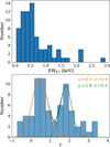 |
Fig. 2 Distribution of EW of the 6.7 keV line (top panel) and X-ray spectral index Γ for 6.7 keV line sources (bottom panel). |
4.2 Sample properties
We fit the spectra of all X-ray point sources detected in the 6.5–7 keV band following the method described in Sect. 3. We selected only sources that showed the presence of a 6.7 keV line above the 2σ confidence level. We detected the Fe XXV line above this threshold in a total of 72 sources. The details of these 72 sources are listed in Table A.1. The top panel of Fig. 2 shows the distribution of EW6.7 for these sources. The bottom panel of Fig. 2 shows the distribution of spectral index Γ, obtained by fitting the spectrum in the 0.2–10 keV band using an absorbed power-law model. The distribution clearly exhibits two peaks at Γ ≃ 0.5 and 1.8, suggesting two distinct source populations. We performed a Kolmogorov-Smirnov (KS) test to determine whether the sample could be drawn from a single normal distribution. The KS test yielded a p-value of 1.5 x 10⁻¹², rejecting the null hypothesis with more than 5σ confidence. To test the alternative hypothesis of two distinct populations, we fit the distribution with two normal distributions and applied the KS test between the original sample and the distribution drawn from the fitted Gaussians. The p-value for this alternative hypothesis is 0.93, indicating the presence of two populations of sources. This becomes even clearer when comparing the Γ and  values of identified sources from SIMBAD, as discussed in Sect. 4.3.
4.2.1 Intensity ratio of ionised Fe lines  vs. EW6.7
We computed the line intensity ratio between Fe XXVI and Fe XXV ( ). Among the 72 sources that show Fe XXV above the 2σ confidence level, 55 emit a strong Fe XXVI line. For 13 sources, only upper limit measurements on the Fe XXVI line were available. For the remaining four sources, the Fe XXVI line measurement was not possible due to insufficient S/N above 6.9 keV. Figure 3 shows the line intensity ratio
  versus EW6.7 for the 68 sources with errors at the 1σ confidence level. In general, the relationship between
  and EW6.7 exhibits a negative trend. For comparison, we also plot the mean values of EW6.7 and line ratio of different mCVs (IPs, polars), non-mCVs (dwarf novae: DNe), and symbiotic systems (SSs) from Xu et al. (2016). The blue and green lines with dots represent the EW6.7 and
  values expected for collisionally ionised plasma at different temperatures. The line intensity ratio is often used to trace the plasma temperature of the material emitting the ionised lines. In general, mCVs like IPs and polars have temperatures much higher than those of non-mCVs (mostly DNe) and ABs. The higher temperature naturally leads to a higher Fe XXVI ions and a lower fraction of Fe XXV ions, resulting in an increased value of
  . Therefore,
  is positively correlated with plasma temperature. The EW6.7 also depends on the temperature. Sources with lower temperatures exhibit larger EW6.7 values than those with very high plasma temperatures because higher temperatures produce more H-like Fe ions relative to He-like ions. Hence, EW6.7 is inversely correlated with temperature. We simulated spectra using XSPEC for a range of plasma temperatures kT. The top panel of Fig. 4 shows the positive correlation of
  with temperature kT indicated by the blue curve, and the negative correlation of EW6.7 with kT highlighted by the red curve. These correlations result in the overall negative trend between
  and EW6.7 observed in Fig. 3, where the smaller values of EW6.7 and the higher value of
  are associated with sources with high plasma temperatures. In contrast, larger values of EW6.7 and smaller values of
  are probably associated with lower temperatures. This trend is also evident in the spectral simulation of ionised plasma shown in the bottom panel of Fig. 4.
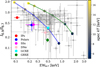 |
Fig. 3 Line intensity ratio |


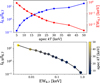 |
Fig. 4 Top panel: relation of EW6.7 and |


4.2.2 Correlation of Γ and EW6.7
If the inverse correlation of versus EW6.7 is driven by temperature, then some level of correlation between EW6.7 and the X-ray spectral slope, Γ, is expected, as Γ is influenced by the temperature of the system. In the upper panel of Fig. 5 we plot EW6.7 versus Γ for the 72 sources. The scatter plot shows an apparent linear positive correlation, suggesting that soft sources with large values of Γ have higher EW6.7 than hard sources with smaller Γ. The correlation is more pronounced when we bin the data with a constant step size of 0.3 keV in EW6.7 (middle panel of Fig. 5). We computed the Pearson correlation coefficient of the grouped data, obtaining a value of 0.99, indicating a strong positive correlation. The correlation has a p-value of 0.0016, indicating that a linear relationship between EW6.7 and Γ is present above the 3a confidence level. Furthermore, fitting the data with a straight line yields a slope of 1.4 and an intercept of 0.2. This linear relationship can be understood by assuming that the X-ray emission from the sources can be modelled with a collisionally ionised plasma model. The bottom panel of Fig. 5 shows a similar linear correlation obtained from spectral simulations of collisionally ionised plasma at different temperatures, where the simulated spectra are fitted with a power-law model. Sources with smaller values of Γ represent a higher plasma temperature, resulting in a lower fraction of Fe XXV atoms and hence lower values of EW6.7. For example, the X-ray spectrum of a source with kT = 5 keV can be modelled by Γ = 2.1 and EW6.7 = 0.9 keV, while a source with kT = 15 keV will have an X-ray spectrum of Γ = 1.5 and EW6.7 = 0.14 keV. Sources with higher values of Γ correspond to very low temperatures, yielding a higher fraction of Fe XXV atoms and higher EW6.7.
The linear correlation between Γ and EW6.7 suggests that the X-ray emission from these sources is coming from a thermal mechanism. Furthermore, the bottom panel of Fig. 5 indicates that in our spectral simulation using the apec model, the highest temperature corresponds to a minimum Γ ∼ 1.3, whereas the top panel shows many sources with Γ below 1. This indicates that a simple model may be insufficient for spectral modelling. Hard sources such as IPs often have local absorption, modelled with a partial covering factor. Furthermore, the physical mechanism that describes the X-ray emission from IPs and polars involves a multi-temperature accretion column, which cannot be accounted for by a single-temperature model such as apec or bremsstrahlung.
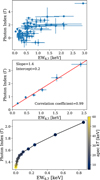 |
Fig. 5 Top panel: scatter plot of photon index Γ vs. EW6.7 of the 72 sources listed in Table A.1. Middle panel: same as the above plot, with data re-binned with an EW step size of 0.3 keV and errors propagated from individual measurement. Bottom panel: linear correlation between Γ vs. EW6.7 obtained from spectral simulation of ionised plasma at different temperatures of solar abundance. |
4.3 Counterpart search and classification
For the classification of the 72 sources, we searched for counterparts in SIMBAD2 within a 3″ distance from XMM-Newton positions. We found counterparts for almost half of the sources (33 of 72). The counterparts can be broadly categorised into three subcategories: CV, high-mass X-ray binary (HMXB), and stellar association. The majority of the CVs and HMXBs were securely identified in our previous work by detecting their X-ray spin periods (Mondal et al. 2024a). In our sample, there are 18 identified CVs which typically have hard X-ray spectra. Of these 18 identified CVs, only two have Γ > 1.0; the rest have X-ray spectral photon indices Γ ≤ 1.0. These sources are shown as blue points in Fig. 6.
In the sample of 72 sources, three are classified as HMXBs. All three have X-ray spectral indices Γ ≳ 1.0, shown as green points in Fig. 6. The HMXBs are powered by wind accretion, and their strongest emission line in their spectra is the Fe Kα emission at 6.4 keV, produced primarily by fluorescence of surrounding neutral material (Torrejón et al. 2010). Some HMXBs exhibit highly variable Fe XXV line emission, while the Fe XXVI line emission is much weaker compared to Fe XXV (Vrtilek et al. 2001; Goldstein et al. 2004; van der Meer et al. 2005; Masetti et al. 2010).
Furthermore, five sources are associated with young stellar objects (YSOs), two associated with RS CVn-type ABs, and six with coronally active stars. All these stellar objects share the common property of having very soft spectra; therefore, we combined them into a single group and designated them as stellar associations. The sources in this category have much softer spectra, with Γ > 1.36, except for one star with Γ = 0.61. These are shown as red points in Fig. 6.
The various source types have different mechanisms for X- ray emission, and among our identified sources, the CVs exhibit a harder spectral shape than the HMXBs and stellar-type sources. Therefore, the higher plasma temperature associated with the harder spectra of CVs leads to a relatively higher  ratio of Fe XXVI emission, relative to the other two types. Figure 6 shows the line intensity ratio
  versus the X-ray spectral index Γ. It is evident from Fig. 6 that all identified CV-type sources cluster in a restricted region with Γ < 1.5 and 0.3 <
  < 1.1. Among the unidentified sources with Γ < 1.5, only one has below 0.3, indicating that the majority of the hard unidentified sources are likely to be CVs. For the unidentified sources, we classify those with Γ < 1.25 as likely CV candidates. In contrast to the identified CVs, the identified stellar-type sources exhibit a wider range of line ratio values, with
  . Furthermore, the stellar-type identified sources show a linear trend of decreasing
  with increasing Γ. This trend likely arises because larger Γ values imply lower plasma temperatures, resulting in a smaller proportion of Fe XXVI relative to Fe XXV line emission.
We also searched for a Gaia counterpart within a 3″ distance from XMM-Newton positions to estimate the distance to the sources using the Gaia parallax. If a counterpart was found, we used the Gaia source ID to determine the distance to the source from Bailer-Jones et al. (2021). The distances to the sources with identified Gaia counterparts, along with the corresponding 2-10 keV X-ray luminosities, are provided in Table A.1.
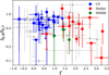 |
Fig. 6 Line ratios vs. the X-ray spectral photon index Γ. The small grey points indicate the unidentified sources. |
5 Discussion
The characteristics of X-ray point sources towards the GC and Galactic disc, and their relative contributions to the GCXE and GRXE, are still unclear. Recently, Koyama & Nobukawa (2024) fitted the GRXE spectra with an assembly of X-ray active stars and compact X-ray objects, which revealed a significant excess at the Kα, Heα, and Lyα lines. These excesses are interpreted as arising from collisional ionisation equilibrium plasma, which is considered an additional emission component from supernova remnants. Furthermore, Warwick et al. (2011) studied the population of faint X-ray sources using XMM-Newton in the Galactic plane, far from the GC (315° < l < 45°). They found that faint X-ray sources can be roughly divided into two categories: soft sources with Γ ∼ 2.5 and hard sources with Γ ∼ 1. The average spectral and Fe-line properties of the hard sources are consistent with the mCVs, and the soft sources are likely associated with relatively nearby coronally active late-type stars, which are identified as bright near-infrared objects within the X-ray positions (Warwick et al. 2014). Subsequently, Warwick (2014) constructed the X-ray luminosity function of the soft and hard sources and found that, in the 6–10 keV band, 80% of the GRXE intensity originates from point sources, the remainder attributable to X-ray scattering in the interstellar medium and/or young Galactic source populations. Recently, Schmitt et al. (2022) attempted to classify sources in the GC by cross-matching Chandra sources with the Gaia EDR3 catalogue, identifying only one third of X-ray point sources, and concluded that the GRXE is produced by optically faint mCVs and DNe. From previous studies (Revnivtsev et al. 2009; Hong 2012; Warwick 2014; Schmitt et al. 2022), it is apparent that in the 6–7 keV band, the vast majority of the GRXE can be resolved into point sources, with mCVs as the primary contributors. The EWs of the 6.4 and 6.9 keV lines of mCVs appear consistent with the GRXE. However, the EW6.7 of mCVs in the solar neighbourhood is a factor of 2–3 times smaller than that of the GRXE. Xu et al. (2016) compared the EW6.7 and  of the GRXE with different classes of known bright sources in the solar neighbourhood, including mCVs (IPs and polars), non-mCVs such as DNe, and ABs. They concluded that all source classes except DNe show average Fe line diagnostics (EW6.7 and
  ) significantly different from those observed in the GRXE (see Fig. 3). Thus, without a major contribution from DNe, no combination of other source classes appears to be able to explain the observed EW6.7 and
  of the GRXE. Therefore, they suggested that the GRXE mostly consists of numerous faint DNe, with mCVs only responsible for the high-flux population of the GRXE. From our Fig. 3 it is evident that in our sample, numerous sources have EW6.7 similar or higher than that of the GCXE or GRXE. This indicates that the discrepancy in EW6.7 between various types of CV populations and the GRXE noted by Xu et al. (2016) can be explained by incorporating these sources into our sample.
In Fig. 6, we see that most of the identified CVs have smaller values of Γ, so the unidentified sources with Γ < 1.25 are strong candidates for CVs. There are 21 unidentified sources with Γ < 1.25. They are most likely magnetic-type CVs as their  values are similar to those of the mCVs, which are much larger than values found in non-mCVs. Among the 21 CV candidates, most have values of
  , except for two sources. Non-mCVs, such as quiescent DNe, have weak 6.9 keV line emission (⟨EW6.9⟩)= 95 ± 18.6 eV; Xu et al. 2016). Therefore, quiescent DNe have a typical
  = 0.27 ± 0.06 (Xu et al. 2016), much lower than the values found in mCVs such as IPs (
 )= 0.71 ± 0.04) and polars (
 )= 0.44 ± 0.14), as illustrated in Fig. 3. Furthermore, in our sample of 18 identified CVs, 13 are classified as mCVs by Mondal et al. (2024a) using spin detection, and for only five is it unknown whether they are magnetic or non-magnetic. However, among the five sources, four have distance measurements from Gaia, which indicate luminosities above 1033 erg s−1, similar to luminosities seen in mCVs; non-mCVs typically have luminosities below 1032 erg s−1 (Suleimanov et al. 2022). The distribution of EW6.7 for the CV sample is shown in Fig. 7. The EW6.7 distribution shows a peak around ∼0.2 keV and an extended tail up to 1 keV. The CV sample has ⟨EW6.7⟩= 415 ± 39 eV, where the error is the standard error of the sample mean. The peak at ∼0.2 keV is likely associated with the typical EW6.7 values observed in nearby mCVs.
The ⟨EW6.7⟩ of our CV sample is more than twice as high as the typical EW6.7 value found in CVs from the solar neighbourhood. There is a possibility that such a high mean value might be due to selection bias, since mean is computed from a sample of sources with Fe XXV line detection significance above 2σ. This could result in a bias such that, for faint sources, only the strongest Fe XXV lines are selected due to low S/N, as the majority of our sources in the CV sample (almost 75%) have 210 keV flux below 10−12 erg s−1 cm−2. This may lead to higher ⟨EW6.7⟩ because only high EW6.7 sources cross the detection threshold above 2σ. In fact, when we plot the 2–10 keV flux versus EW6.7 for all our sources with Γ < 1.25, we observe a negative correlation (Fig. 8) suggesting that only the fainter sources with larger EW6.7 are selected due to the choice of detection threshold. If there is indeed a selection bias, then one might also expect to detect bright sources with 2–10 keV flux above 10−12 erg s−1 cm−2 and EW6.7 > 0.4 keV, which are not present in Fig. 8. This indicates that the inverse trend of flux versus EW6.7 is likely not due to selection bias. This becomes clearer when we stack the spectra of all point sources detected in the 6.5–7 keV band and measure the EW6.7 of the stacked spectra. The inverse trend of flux versus EW6.7 of the hard X-ray sources is likely driven by their distance, as indicated by the positive correlation between distance versus EW6.7, shown in the top panel of Fig. 9. Furthermore, the bottom panel of Fig. 9 shows that EW6.7 is independent of luminosity. For solar neighbourhood CVs (including mCVs and non-mCVs) the luminosity versus EW6.7 displays an inverse trend, driven by the fact that non-mCVs, such as DNe, have much lower luminosity (typically below 1032 erg s−1) and much higher EW6.7 than mCVs, such as IPs and polars. This is illustrated in Fig. 7 of Xu et al. (2016). The bottom panel of Fig. 9 shows that all sources, except one, have 2–10 keV X-ray luminosities above 2 x 1032 erg s−1, consistent with the luminosities of mCVs (IPs and polars; Suleimanov et al. 2022), rather than non-mCVs, which typically have X- ray luminosities a factor of 10 to 100 times lower than those of mCVs. In addition, these hard sources have a line ratio  , much higher than non-mCVs, which suggests that most of these sources are likely mCVs.
We computed the stacked spectra of all sources detected in the 6.5–7 keV band with ML>14. We then stacked the spectra of the sources according to different groups based on their 2–10 keV flux. To separate the two populations of sources, we defined a cut in hardness ratio (HR), with HR > -0.2 and HR ≤ -0.2, for the hard (Γ < 1.25) and soft (Γ ≥ 1.25) sources, respectively. The hardness ratio is defined as  , where C denotes the net count in the respective energy band. Figure 10 shows the stacked spectra of sources with HR > -0.2 for different flux groups. The stacked spectra are fitted with a power-law continuum and three Gaussians at 6.4, 6.7, and 6.9 keV for the Fe complex. The stacked spectra of bright sources with 2–10 keV flux > 10−12 erg s−1 cm−2 do not show the presence of ionised Fe XXV and Fe XXVI lines; however, there is a weak indication that the neutral 6.4 keV line is present. The Fe complex becomes more prominent in the stacked spectra of sources with 2–10 keV flux <10−12 erg s−1 cm−2. From Fig. 10 it is clear that the strength of the Fe XXV line relative to the neutral Fe Kα line and the Fe XXVI line increases as we stack sources with fainter flux. Figure 11 shows the EW6.7 obtained from the stacked spectra as a function of the 2–10 keV mean flux, suggesting that the faint sources have significantly larger EW6.7 compared to the brighter sources, as seen in Fig. 8. This ensures that the large ⟨EW6.7⟩ of our identified and candidate CV sources is less likely due to a selection bias, but is due to the fact that faint sources are more likely to have higher EW6.7.
The extended tail of our CV candidate sample, leading to a higher ⟨EW6.7⟩= 415 ± 39 eV, can be explained by assuming that they have a metallicity higher than solar. For example, in the solar neighbourhood, a typical CV with a plasma temperature of 15 keV has an EW6.7 of ∼0.14 keV. However, for the same plasma temperature, assuming an iron abundance of 2.5 times solar yields an EW6.7 of 0.3 keV. Conversely, for a plasma temperature of 10 keV, EW6.7 = 0.35 and 0.72 keV for abundance values 1.0, and 2.5, respectively, as shown in Fig. 12 through spectral simulation. Figure 12 indicates that the large ⟨EW6.7⟩ of 415 eV can be explained by assuming a relatively low plasma temperature of 10–12 keV and an abundance of 1–2 times solar. At higher plasma temperatures, this will require a significantly higher abundance, which is unlikely.
We detected a significant number of sources that emit a strong 6.7 keV line and have a very soft X-ray spectrum. Figure 13 shows the EW6.7 distribution for these soft sources. The mean EW6.7, with standard error, is ⟨EW6.7⟩= 1.0 ± 0.1 keV. We identified counterparts for 13 soft sources within a distance of 3" from the XMM-Newton position. Two are associated with RS CVn-type stars, a class of variable binary stars known to emit strong coronal X-ray emission and 6.7 keV line emission (Audard et al. 2001). The X-ray continuum emission from these types of sources is typically described by two temperature components: a line-emitting plasma with a characteristic temperature of ∼0.5 keV, and a Bremsstrahlung continuum of 2–8 keV (Swank et al. 1981). The RS CVn ABs show transient behaviour in the Fe XXV line; however, the EW6.7 is much larger during flare events (Mewe et al. 1997; Güdel et al. 1999; Inoue et al. 2024). Furthermore, five of the 13 sources with counterparts are classified as young stellar objects (YSOs), and six are massive coronally active stars. It is therefore difficult to determine the true nature of the sources with soft X-ray spectra (Γ ≥ 1.25) and large EW6.7, as this combination of spectral properties is observed across several different source classes. Active binary stars such as RS CVn and coronally active stars such as YSOs show a strong 6.7 keV line; however, their X-ray luminosities are much lower (<1032 erg s−1). Massive WR-OB binary stars also emit EW6.7 > 1 keV, originating from windwind collisions, with 2–10 keV luminosities reaching up to 1035 erg s−1. It is also not uncommon for polars to have a similar spectrum shape of Γ > 1.25, while IPs typically exhibit much harder spectra. For example, XMM-Newton detected such a system toward the GC (XMM J174544-2913.0) with  and
and  keV (Sakano et al. 2005). Many polar-type systems detected by ASCA also exhibit Γ ∼ 2 and EW6.7 above 1 keV (AX J2315-592, Misaki et al. 1996; RX J1802.1+1804, Ishida et al. 1998; AX J1842.8-0423, Terada et al. 1999). The nature of XMM J174544-2913.0 and AX J1842.8-0423 remains unclear due to their transient X-ray emission; however, the two other systems are confirmed polars. Typically, mCVs such as polars in the solar neighbourhood have much lower EW6.7. Terada et al. (2004) proposed that the large EW6.7 observed in polars detected by ASCA, results from collimation of Fe XXV line photons along the accretion column axis due to resonance scattering, which may occur in the case of a pole-on inclination.
We compared the ⟨EW6.7⟩ and  of the hard (Γ < 1.25) and soft sources (Γ ≥ 1.25) with the GCXE and GRXE. The luminosity inferred using Gaia distances and the line ratio
  of the hard sources suggest that they are likely to be mCVs; however, the ⟨EW6.7⟩ of these sources is significantly higher than that of solar neighbourhood mCVs and approaches values seen in the GCXE and GRXE. This indicates that the GCXE and GRXE can have significant contributions from candidate mCVs with large EW6.7. This finding contrasts with earlier studies that proposed non-mCVs as the major contributors to the GRXE, based on comparisons of the Fe emission line properties of sources in the solar neighbourhood with those observed in the GRXE (Xu et al. 2016; Schmitt et al. 2022). The sensitivity limit for point source detection in our survey is around ∼10−14 erg s−1 cm−2. Furthermore, almost ∼50% of our sample in the 6.5–7 keV band consists of hard sources, most of which are likely mCVs. This indicates that among the sources with a flux of 10−14 erg s−1 cm−2 or greater that contribute to the GDXE in the 6.5–7 keV band, nearly half originate from mCVs, with the remainder contributed by soft sources such as non-mCVs, ABs, YSOs, and coronally active stars. In addition, IPs are likely to contribute to the higher flux level of ∼8 x 10⁻¹⁴ erg s−1 cm−2 or higher. Figure 14 shows the sample mean and 1σ standard deviation. The ⟨EW6.7⟩ and
  measurements for both the CV population and soft sources are consistent with those of the GCXE within 1 σ. This indicates that the GCXE can be explained by the hard CV population, the soft sources, or a combination of both. On the other hand, in contrast to the GCXE, the GRXE exhibits a much lower
  than the CV population. However, the line intensity ratio
  of the GRXE is consistent within the 1σ measurement of the soft sources. This indicates that low flux (<1.8 × 10⁻¹³ erg s−1 cm−2) soft sources, such as ABs and coro- nally active stars, may contribute a significant amount to the GRXE.
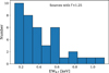 |
Fig. 7 Distribution of EW6.7 for identified CVs and candidate CVs characterised by Γ < 1.25. |
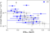 |
Fig. 8 2–10 keV flux vs. EW6.7 for sources with Γ < 1.25. Blue points indicate sources identified as CVs and grey points represent unidentified CV candidates. |
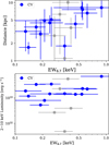 |
Fig. 9 Distance (top panel) and 2–10 keV luminosity (bottom panel) vs. EW6.7 for sources with Γ < 1.25 for which a distance estimation was possible using Gaia parallax. Blue points indicate sources identified as CVs, while grey points represent unidentified CV candidates. |
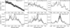 |
Fig. 10 Stacked spectra of point sources with HR>-0.2 and ML>14 in the 6.5–7 keV band for different flux groups. The spectra were fitted by a power-law continuum and three Gaussian lines at 6.4, 6.7, and 6.9 keV for the Fe complex. |
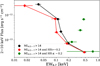 |
Fig. 11 Stacked-spectra EW6.7 for point sources in grouped by 210 keV flux. All sources detected with ML>14 in the 6.5–7 keV band are considered (black line-connected dots). Red and green points correspond to sources with HR > -0.2 and HR ≤ -0.2, respectively. The 2-10 keV observed flux represents the mean flux of each group, and the error bars show the standard error of the mean. The EW6.7 errors are at the 1σ confidence level obtained from XSPEC. |
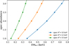 |
Fig. 12 Dependence of EW6.7 for three different plasma temperatures: 10, 12, and 15 keV. Dots indicate abundance values used in spectral simulations with an apec model, and the EW6.7 values were estimated by fitting the simulated spectra using a model composed of power-law plus Gaussian at 6.7 keV with width fixed to zero eV. |
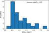 |
Fig. 13 Distribution of EW6.7 for identified stellar-type sources and unidentified sources with Γ ≥ 1.25. |
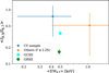 |
Fig. 14 Comparison of the mean EW6.7 and |

6 Conclusions
We aimed to characterise the sources contributing to the Galactic diffuse X-ray emission in the 6.7 keV band. The sample of sources contributing to this Galactic diffuse X-ray emission consists primarily of CVs, coronally active stars, and ABs. Previous studies suggested that the 6.7 keV line emission of the Galactic diffuse X-ray emission originates primarily from mCVs. However, the EW6.7 and line intensity ratio  of the GCXE and GRXE do not match those of the mCVs. To address this discrepancy, we measured the X-ray spectral slope Γ, EW6.7, and
  for a substantial number of individual sources in the inner Galactic disc. The main conclusions of this study are as follows.
We detected the Fe XXV line above the 2σ confidence level in a sample of 72 sources. The EW6.7 ranges from a few hundred eV to ∼3 keV. The sample consists primarily of two populations: hard and soft sources, characterised by an X-ray spectral slope Γ below and above 1.25, respectively.
The EW6.7 correlates with the X-ray spectral slope, Γ. The harder sources with smaller values of Γ have a lower EW6.7 line than the softer sources with large Γ.
The vast majority of hard sources are identified with known CVs. The X-ray spectral slope Γ and the line intensity ratio
 of the subsample suggest that they are prime candidates for CV. The ⟨EW6.7⟩ of these harder CV-type sources is 415 ± 39 eV, significantly higher than the typical EW6.7 value of ∼170 eV found in CVs in the solar neighbourhood. This suggests that the iron abundance of these harder sources must be 1-2 times the solar value, with a plasma temperature of 10–12 keV.
The soft source sample is associated with stellar-like activities and has an ⟨EW6.7⟩= 1.1 ± 0.1 keV. These sources have a mean spectral index Γ ∼ 1.8, and their ⟨EW6.7⟩ values are consistent with those observed in coronally active stars, AB-like RS CVn stars, and YSOs.
Galactic centre X-ray emission can be explained by a mixture of CVs with higher solar abundance and a contribution from soft sources. However, the soft sources may contribute significantly to Galactic ridge X-ray emission.
Acknowledgements
SM, GP, and TB acknowledge support from Bando per il Finanziamento della Ricerca Fondamentale 2022 dell’Istituto Nazionale di Astrofisica (INAF): GO Large program and from the Framework per l’Attrazione e il Rafforzamento delle Eccellenze (FARE) per la ricerca in Italia (R20L5S39T9). GP also acknowledges financial support from the European Research Council (ERC) under the European Union’s Horizon 2020 research and innovation program HotMilk (grant agreement No. 865637). MM gratefully acknowledges support for this work from NASA ADAP grant 80NSSC24K0639. We thank the referee for the constructive comments, corrections, and suggestions that significantly improved the manuscript.
Appendix A Additional tables
The various details of the X-ray sources emitting Fe XXV line.
References
- Anastasopoulou, K., Ponti, G., Sormani, M. C., et al. 2023, A&A, 671, A55 [NASA ADS] [CrossRef] [EDP Sciences] [Google Scholar]
- Arnaud, K. A. 1996, in Astronomical Data Analysis Software and Systems V, eds. G. H. Jacoby, & J. Barnes, Astronomical Society of the Pacific Conference Series, 101, 17 [NASA ADS] [Google Scholar]
- Audard, M., Güdel, M., & Mewe, R. 2001, A&A, 365, L318 [NASA ADS] [CrossRef] [EDP Sciences] [Google Scholar]
- Bailer-Jones, C. A. L., Rybizki, J., Fouesneau, M., Demleitner, M., & Andrae, R. 2021, AJ, 161, 147 [Google Scholar]
- Belmont, R., Tagger, M., Muno, M., Morris, M., & Cowley, S. 2005, ApJ, 631, L53 [NASA ADS] [CrossRef] [Google Scholar]
- Cooke, B. A., Griffiths, R. E., & Pounds, K. A. 1969, Nature, 224, 134 [NASA ADS] [CrossRef] [Google Scholar]
- Cropper, M. 1990, Space Sci. Rev., 54, 195 [CrossRef] [Google Scholar]
- Ezuka, H., & Ishida, M. 1999, ApJS, 120, 277 [NASA ADS] [CrossRef] [Google Scholar]
- Goldstein, G., Huenemoerder, D. P., & Blank, D. 2004, AJ, 127, 2310 [Google Scholar]
- Gordon, C., & Arnaud, K. 2021, PyXspec: Python interface to XSPEC spectral- fitting program, Astrophysics Source Code Library [record ascl:2101.014] [Google Scholar]
- Güdel, M., Linsky, J. L., Brown, A., & Nagase, F. 1999, ApJ, 511, 405 [Google Scholar]
- Hellier, C., & Mukai, K. 2004, MNRAS, 352, 1037 [NASA ADS] [CrossRef] [Google Scholar]
- Hellier, C., Mukai, K., & Osborne, J. P. 1998, MNRAS, 297, 526 [Google Scholar]
- Hong, J. 2012, MNRAS, 427, 1633 [NASA ADS] [CrossRef] [Google Scholar]
- Inoue, S., Iwakiri, W. B., Enoto, T., et al. 2024, ApJ, 969, L12 [Google Scholar]
- Ishida, M., Greiner, J., Remillard, R. A., & Motch, C. 1998, A&A, 336, 200 [Google Scholar]
- Jansen, F., Lumb, D., Altieri, B., et al. 2001, A&A, 365, L1 [NASA ADS] [CrossRef] [EDP Sciences] [Google Scholar]
- Kellogg, E., Gursky, H., Murray, S., Tananbaum, H., & Giacconi, R. 1971, ApJ, 169, L99 [Google Scholar]
- Koyama, K. 2018, PASJ, 70, R1 [Google Scholar]
- Koyama, K., & Nobukawa, M. 2024, ApJ, 961, 205 [Google Scholar]
- Masetti, N., Landi, R., Sguera, V., et al. 2010, A&A, 511, A48 [NASA ADS] [CrossRef] [EDP Sciences] [Google Scholar]
- Mewe, R., Kaastra, J. S., van den Oord, G. H. J., Vink, J., & Tawara, Y. 1997, A&A, 320, 147 [Google Scholar]
- Misaki, K., Terashima, Y., Kamata, Y., et al. 1996, ApJ, 470, L53 [Google Scholar]
- Mondal, S., Ponti, G., Haberl, F., et al. 2022, A&A, 666, A150 [NASA ADS] [CrossRef] [EDP Sciences] [Google Scholar]
- Mondal, S., Ponti, G., Haberl, F., et al. 2023, A&A, 671, A120 [NASA ADS] [CrossRef] [EDP Sciences] [Google Scholar]
- Mondal, S., Ponti, G., Bao, T., et al. 2024a, A&A, 686, A125 [NASA ADS] [CrossRef] [EDP Sciences] [Google Scholar]
- Mondal, S., Ponti, G., Filor, L., et al. 2024b, A&A, 689, A172 [NASA ADS] [CrossRef] [EDP Sciences] [Google Scholar]
- Mukai, K. 2017, PASP, 129, 062001 [Google Scholar]
- Nobukawa, M., Uchiyama, H., Nobukawa, K. K., Yamauchi, S., & Koyama, K. 2016, ApJ, 833, 268 [NASA ADS] [CrossRef] [Google Scholar]
- Patterson, J. 1994, PASP, 106, 209 [Google Scholar]
- Ponti, G., Hofmann, F., Churazov, E., et al. 2019, Nature, 567, 347 [Google Scholar]
- Ponti, G., Morris, M. R., Terrier, R., & Goldwurm, A. 2013, in Cosmic Rays in Star-Forming Environments, eds. D. F. Torres & O. Reimer, Astrophysics and Space Science Proceedings, 34, 331 [NASA ADS] [CrossRef] [Google Scholar]
- Ponti, G., Morris, M. R., Terrier, R., et al. 2015, MNRAS, 453, 172 [Google Scholar]
- Porquet, D., Dubau, J., & Grosso, N. 2010, Space Sci. Rev., 157, 103 [Google Scholar]
- Revnivtsev, M., Sazonov, S., Gilfanov, M., Churazov, E., & Sunyaev, R. 2006, A&A, 452, 169 [NASA ADS] [CrossRef] [EDP Sciences] [Google Scholar]
- Revnivtsev, M., Sazonov, S., Churazov, E., et al. 2009, Nature, 458, 1142 [Google Scholar]
- Sakano, M., Warwick, R. S., Decourchelle, A., & Wang, Q. D. 2005, MNRAS, 357, 1211 [NASA ADS] [CrossRef] [Google Scholar]
- Schmitt, J. H. M. M., Czesla, S., Schneider, P. C., Freund, S., & Robrade, J. 2022, A&A, 661, A88 [NASA ADS] [CrossRef] [EDP Sciences] [Google Scholar]
- Strüder, L., Briel, U., Dennerl, K., et al. 2001, A&A, 365, L18 [Google Scholar]
- Suleimanov, V. F., Doroshenko, V., & Werner, K. 2022, MNRAS, 511, 4937 [NASA ADS] [CrossRef] [Google Scholar]
- Swank, J. H., White, N. E., Holt, S. S., & Becker, R. H. 1981, ApJ, 246, 208 [Google Scholar]
- Tanaka, Y. 2002, A&A, 382, 1052 [NASA ADS] [CrossRef] [EDP Sciences] [Google Scholar]
- Terada, Y., Kaneda, H., Makishima, K., et al. 1999, PASJ, 51, 39 [Google Scholar]
- Terada, Y., Ishida, M., & Makishima, K. 2004, PASJ, 56, 533 [Google Scholar]
- Torrejón, J. M., Schulz, N. S., Nowak, M. A., & Kallman, T. R. 2010, ApJ, 715, 947 [CrossRef] [Google Scholar]
- Turner, M. J. L., Abbey, A., Arnaud, M., et al. 2001, A&A, 365, L27 [CrossRef] [EDP Sciences] [Google Scholar]
- Uchiyama, H., Nobukawa, M., Tsuru, T. G., & Koyama, K. 2013, PASJ, 65, 19 [NASA ADS] [Google Scholar]
- van der Meer, A., Kaper, L., di Salvo, T., et al. 2005, A&A, 432, 999 [NASA ADS] [CrossRef] [EDP Sciences] [Google Scholar]
- Vrtilek, S. D., Raymond, J. C., Boroson, B., et al. 2001, ApJ, 563, L139 [NASA ADS] [CrossRef] [Google Scholar]
- Warwick, R. S. 2014, MNRAS, 445, 66 [CrossRef] [Google Scholar]
- Warwick, R. S., Pye, J. P., & Fabian, A. C. 1980, MNRAS, 190, 243 [Google Scholar]
- Warwick, R. S., Turner, M. J. L., Watson, M. G., & Willingale, R. 1985, Nature, 317, 218 [NASA ADS] [CrossRef] [Google Scholar]
- Warwick, R. S., Pérez-Ramírez, D., & Byckling, K. 2011, MNRAS, 413, 595 [Google Scholar]
- Warwick, R. S., Byckling, K., & Pérez-Ramírez, D. 2014, MNRAS, 438, 2967 [Google Scholar]
- Watson, M. G., Willingale, R., Grindlay, J. E., & Hertz, P. 1981, ApJ, 250, 142 [CrossRef] [Google Scholar]
- Webb, N. A., Coriat, M., Traulsen, I., et al. 2020, A&A, 641, A136 [NASA ADS] [CrossRef] [EDP Sciences] [Google Scholar]
- Wilms, J., Allen, A., & McCray, R. 2000, ApJ, 542, 914 [Google Scholar]
- Worrall, D. M., Marshall, F. E., Boldt, E. A., & Swank, J. H. 1982, ApJ, 255, 111 [Google Scholar]
- Xu, X.-j., Wang, Q. D., & Li, X.-D. 2016, ApJ, 818, 136 [NASA ADS] [CrossRef] [Google Scholar]
- Yamauchi, S., Nobukawa, K. K., Nobukawa, M., Uchiyama, H., & Koyama, K. 2016, PASJ, 68, 59 [NASA ADS] [CrossRef] [Google Scholar]
All Tables
All Figures
|
Fig. 1 Top panel: longitude profile of total emission (point sources plus unresolved emission) in the 6.5–7.0 keV range, integrated over -0.8° ≤ b ≤ 0.8° (black curve). The red curve shows the contribution from point sources detected with ML > 14 in the 1–12 keV band. Bottom panel: percentage of the total 6.5–7.0 keV emission resolved by X-ray point sources. |
| In the text | |
|
Fig. 2 Distribution of EW of the 6.7 keV line (top panel) and X-ray spectral index Γ for 6.7 keV line sources (bottom panel). |
| In the text | |
|
Fig. 3 Line intensity ratio |
| In the text | |
|
Fig. 4 Top panel: relation of EW6.7 and |
| In the text | |
|
Fig. 5 Top panel: scatter plot of photon index Γ vs. EW6.7 of the 72 sources listed in Table A.1. Middle panel: same as the above plot, with data re-binned with an EW step size of 0.3 keV and errors propagated from individual measurement. Bottom panel: linear correlation between Γ vs. EW6.7 obtained from spectral simulation of ionised plasma at different temperatures of solar abundance. |
| In the text | |
|
Fig. 6 Line ratios vs. the X-ray spectral photon index Γ. The small grey points indicate the unidentified sources. |
| In the text | |
|
Fig. 7 Distribution of EW6.7 for identified CVs and candidate CVs characterised by Γ < 1.25. |
| In the text | |
|
Fig. 8 2–10 keV flux vs. EW6.7 for sources with Γ < 1.25. Blue points indicate sources identified as CVs and grey points represent unidentified CV candidates. |
| In the text | |
|
Fig. 9 Distance (top panel) and 2–10 keV luminosity (bottom panel) vs. EW6.7 for sources with Γ < 1.25 for which a distance estimation was possible using Gaia parallax. Blue points indicate sources identified as CVs, while grey points represent unidentified CV candidates. |
| In the text | |
|
Fig. 10 Stacked spectra of point sources with HR>-0.2 and ML>14 in the 6.5–7 keV band for different flux groups. The spectra were fitted by a power-law continuum and three Gaussian lines at 6.4, 6.7, and 6.9 keV for the Fe complex. |
| In the text | |
|
Fig. 11 Stacked-spectra EW6.7 for point sources in grouped by 210 keV flux. All sources detected with ML>14 in the 6.5–7 keV band are considered (black line-connected dots). Red and green points correspond to sources with HR > -0.2 and HR ≤ -0.2, respectively. The 2-10 keV observed flux represents the mean flux of each group, and the error bars show the standard error of the mean. The EW6.7 errors are at the 1σ confidence level obtained from XSPEC. |
| In the text | |
|
Fig. 12 Dependence of EW6.7 for three different plasma temperatures: 10, 12, and 15 keV. Dots indicate abundance values used in spectral simulations with an apec model, and the EW6.7 values were estimated by fitting the simulated spectra using a model composed of power-law plus Gaussian at 6.7 keV with width fixed to zero eV. |
| In the text | |
|
Fig. 13 Distribution of EW6.7 for identified stellar-type sources and unidentified sources with Γ ≥ 1.25. |
| In the text | |
|
Fig. 14 Comparison of the mean EW6.7 and |
| In the text | |
Current usage metrics show cumulative count of Article Views (full-text article views including HTML views, PDF and ePub downloads, according to the available data) and Abstracts Views on Vision4Press platform.
Data correspond to usage on the plateform after 2015. The current usage metrics is available 48-96 hours after online publication and is updated daily on week days.
Initial download of the metrics may take a while.