| Issue |
A&A
Volume 671, March 2023
|
|
|---|---|---|
| Article Number | A120 | |
| Number of page(s) | 9 | |
| Section | Stellar structure and evolution | |
| DOI | https://doi.org/10.1051/0004-6361/202245553 | |
| Published online | 14 March 2023 | |
Discovery of periodicities in two highly variable intermediate polars towards the Galactic centre
1
INAF – Osservatorio Astronomico di Brera, Via E. Bianchi 46, 23807 Merate, LC, Italy
e-mail: samaresh.mondal@inaf.it
2
Max-Planck-Institut für extraterrestrische Physik, Gießenbachstraße 1, 85748 Garching, Germany
3
Columbia Astrophysics Laboratory, Columbia University, Columbia, NY 10027, USA
4
Institute of Space Sciences (ICE, CSIC), Campus UAB, Carrer de Can Magrans s/n, 08193 Barcelona, Spain
5
Institut d’Estudis Espacials de Catalunya (IEEC), Carrer Gran Capitá 2-4, 08034 Barcelona, Spain
6
Department of Physics and Astronomy, University of California, Los Angeles, CA 90095-1547, USA
7
Center for Astrophysics, Harvard & Smithsonian, 60 Garden Street, Cambridge, MA 20138, USA
Received:
25
November
2022
Accepted:
23
January
2023
Aims. We performed a systematic analysis of X-ray point sources within 1.°5 of the Galactic centre using archival XMM-Newton data. While doing so, we discovered Fe Kα complex emission and pulsation in two highly variable sources, 4XMM J174917.7–283329 and 4XMM J174954.6–294336. In this work we report the findings of the X-ray spectral and timing studies.
Methods. We performed detailed spectral modelling of the sources and searched for pulsation in the light curves using Fourier timing analysis. We also searched for multi-wavelength counterparts for the characterization of the sources.
Results. The X-ray spectrum of 4XMM J174917.7–283329 shows the presence of complex Fe K emission in the 6–7 keV band. The equivalent widths of the 6.4 and 6.7 keV lines are 99−72+84 and 220−140+160 eV, respectively. The continuum is fitted by a partially absorbed apec model with a plasma temperature of kT = 13−2+10 keV. The inferred mass of the white dwarf (WD) is 0.9−0.2+0.3 M⊙. We detected pulsations with a period of 1212 ± 3 s and a pulsed fraction of 26 ± 6%. The light curves of 4XMM J174954.6–294336 display an asymmetric eclipse and dipping behaviour. To date, this is only the second known intermediate polar to show a total eclipse in X-rays. The spectrum of the sources is characterized by a power-law model with photon index Γ = 0.4 ± 0.2. The equivalent widths of the iron fluorescent (6.4 keV) and Fe XXV (6.7 keV) lines are 171−79+99 and 136−81+89 eV, respectively. The continuum is described by emission from optically thin plasma with a temperature of kT ∼ 35 keV. The inferred mass of the WD is 1.1−0.3+0.2 M⊙. We detect coherent pulsations from the source with a period of 1002 ± 2 s. The pulsed fraction is 66 ± 15%.
Conclusions. The spectral modelling indicates the presence of intervening clouds with a high absorbing column density in front of both sources. The detected periodic modulations in the light curves are likely associated with the spin period of WDs in magnetic cataclysmic variables. The measured spin period, hard photon index, and equivalent width of the fluorescent Fe Kα line are consistent with the values found in intermediate polars. 4XMM J174954.6–294336 has already been classified as an intermediate polar, and we suggest that 4XMM J174917.7–283329 is a new intermediate polar. The X-ray eclipses in 4XMM J174954.6–294336 are most likely caused by a low-mass companion star obscuring the central X-ray source. The asymmetry in the eclipse is likely caused by a thick bulge that intercepts the line of sight during the ingress phase but not during the egress phase located behind the WD along the line of sight.
Key words: X-rays: binaries / Galaxy: center / Galaxy: disk / white dwarfs / novae / cataclysmic variables
© The Authors 2023
 Open Access article, published by EDP Sciences, under the terms of the Creative Commons Attribution License (https://creativecommons.org/licenses/by/4.0), which permits unrestricted use, distribution, and reproduction in any medium, provided the original work is properly cited.
This article is published in open access under the Subscribe to Open model. Subscribe to A&A to support open access publication.
1. Introduction
Accreting white dwarf (WD) binaries are abundant in our Universe (see Mukai 2017, for a recent review). They are a common endpoint of intermediate- and low-mass stars, and many stars are born in a binary system with small separations that goes through one or more mass transfer phases. Accreting WD binaries are categorized into two types, mainly on the basis of the companion star, which feeds the central X-ray source via Roche lobe overflow. Cataclysmic variables (CVs) have an early-type main-sequence donor, and symbiotic systems have a late-type giant donor. Understanding the long-term evolution of CVs is necessary for studying the progenitors of Type Ia supernovae and for future detections of gravitational wave sources by the Laser Interferometer Space Antenna in the millihertz band (Meliani et al. 2000; Zou et al. 2020). Furthermore, CVs are categorized into two types, non-magnetic and magnetic. Most of the hard X-ray emission from the Galactic centre (GC) is expected to be produced by magnetic CVs (Revnivtsev et al. 2009; Hong et al. 2009). In magnetic CVs, the matter from the companion star is funnelled through the magnetic field lines to the polar regions of the WD (Cropper 1990; Patterson 1994). The infalling material reaches a supersonic speed of 3000–10 000 km s−1, creating a shock front above the star and emitting thermal X-rays (Aizu 1973). There are two types of magnetic CVs: intermediate polars (IPs) and polars. The former have a non-synchronous orbit with a WD surface magnetic field strength of ∼0.1–10 MG; they emit an ample amount of hard X-rays (20–40 keV). Polars are magnetically locked binary systems that have synchronized orbits with a strong magnetic field of 10–200 MG. Polars have softer X-ray spectra, kT ∼ 5 − 10 keV, due to faster cyclotron cooling (Mukai 2017).
A large number of CVs have been detected through all-sky surveys, such as those performed by ROSAT (Beuermann et al. 1999), INTEGRAL (Barlow et al. 2006), and Swift-BAT (Baumgartner et al. 2013). The 77-month Swift-BAT catalogue, whose sky coverage is relatively uniform, lists around 81, roughly half of which are confirmed to be IPs (Baumgartner et al. 2013). There are also deeper surveys that focus on a small part of the sky; for example, Pretorius et al. (2007) exploited the ROSAT all-sky survey, which was deeper near the north ecliptic pole, to infer the space density of CVs. Many star clusters are also prime targets for finding CVs. Gosnell et al. (2012) discovered a candidate CV in the metal-rich open cluster NGC 6819 using XMM-Newton. Some globular clusters are believed to host a large number of CVs; for example, among the X-ray sources in 47 Tuc (Grindlay et al. 2001a), about 30 are considered likely CVs (Edmonds et al. 2003b,a), and in the globular cluster NGC 6397 nine are likely to be CVs (Grindlay et al. 2001b).
Cataclysmic variables have recently been discussed many times in the context of the GC (Krivonos et al. 2007; Revnivtsev et al. 2009; Hong 2012; Ponti et al. 2013; Perez et al. 2015; Hailey et al. 2016). The diffuse hard X-ray emission in the GC and in the disk (the latter is termed Galactic ridge X-ray emission; Warwick et al. 1985) is from a population of unresolved, faint point sources that includes CVs (Revnivtsev et al. 2009; Yamauchi et al. 2016). However, the contribution from different types of sources and different types of CVs is still an open question. The only unambiguous way to constrain the CV population in the GC, Galactic ridge, and Galactic bulge is to analyse the individual X-ray point sources using spectra and light curves and identify them. Furthermore, estimating the X-ray-to-optical flux ratio by finding multi-wavelength counterparts can help determine the source type. Muno et al. (2003) detected 2350 X-ray point sources in the 17′×17′ field around Sgr A* and found that more than half of the sources are very hard, with photon index Γ < 1, which indicates that they are magnetic CVs. Yuasa et al. (2012) fitted the spectra of the Galactic ridge and bulge regions with a two-component spectral model and found the hard spectral component to be consistent with magnetic CVs of average mass  .
.
We have been systematically studying X-ray point sources in the GC to understand the different types of X-ray binary populations. While doing this analysis, we found two relatively faint sources that have iron complex emission in their X-ray spectra and periodicities in their light curves. In this paper we report the X-ray spectral modelling, periodicities, and characterization of the two X-ray point sources in the GC. The coordinates of the sources are (α, δ)J200 = (17h49m17 7, –28°33′29″) and (17h49m54
 6, –29°43′36″); both of these sources are listed in the 4XMM-DR11 catalogue, as 4XMM J174917.7–283329 and 4XMM J174954.6–294336 (Webb et al. 2020). 4XMM J174917.7–283329 is a newly identified point source for which iron 6.4 and 6.7 keV lines and pulsations in the X-ray light curves have been detected. The source 4XMM J174954.6–294336 was first observed by Chandra during the Bulge Latitude Survey and then detected in the Galactic Bulge Survey (GBS; Jonker et al. 2014); it was later detected by Swift and XMM-Newton. An association of a faint optical counterpart with an orbital period of 0.3587 days was identified by Udalski et al. (2012). A periodicity of 503.3 s was also detected in the optical light curve, which was interpreted as a spin period (Johnson et al. 2017). In this paper we provide the actual spin period of the WD.
2. Observations and data reduction
This work is based on archival XMM-Newton observations of the GC (Ponti et al. 2015, 2019). The details of the observations are listed in Table 1. The observation data files were processed using the XMM-Newton (Jansen et al. 2001) Science Analysis System (SAS, v19.0.0)1. We used the SAS task barycen to apply the barycentre correction to the event arrival times. We only selected events with PATTERN ≤ 4 for the EPIC-pn detector and PATTERN ≤ 12 for the EPIC-MOS1 and MOS2 detectors. The source and background products were extracted from circular regions of 25″ radius. The background products were extracted from a source-free area. The spectrum from each detector (pn, MOS1, and MOS2) was grouped to have a minimum of 20 counts in each energy bin. The spectral fitting was performed in XSPEC (Arnaud et al. 1996), and we applied the χ2 statistic. We fitted the spectra from observations of the EPIC-pn, MOS1, and MOS2 detectors simultaneously. While doing so, we added a constant term for cross-calibration uncertainties, fixed to unity for EPIC-pn and allowed to vary for MOS1 and MOS2. The best-fit parameters are listed in Table 2 with the quoted errors at the 90% significance level.
Details of the observations.
Best-fit parameters of the fitted models.
3. Results
3.1. X-ray spectra
We performed a detailed spectral analysis of the sources 4XMM J174917.7–283329 and 4XMM J174954.6–294336. We tested various phenomenological models to fit the spectra as well as a physical model to constrain the mass of the central WD. The results from the spectral fitting are described in the following subsections. All the spectral fitting models are convolved with a Galactic absorption component, tbabs, with the photoionization cross-sections and abundance values from Wilms et al. (2000).
3.1.1. 4XMM J174917.7–283329
The source was observed three times by XMM-Newton. The observations done on 22 September 2006 (ObsID 0410580401) and 26 September 2006 (ObsID 0410580501) were in timing mode and pointed at IGR J17497–2821, so the source was outside the field of view of the EPIC-pn and MOS1 detectors. In the case of the MOS2 detector, the source was marginally detected due to the high background and low flux state of the source. Hence, we used ObsIDs 0410580401 and 0410580501 to estimate the flux of the source only. The same field was later observed by XMM-Newton on 07 October 2017 (ObsID 0801681301), when the source was brighter and clearly detected by all three detectors. We used spectra from this observation for our detailed spectral modelling.
First, we fitted the spectra with a simple absorbed power-law model. Results from this fit indicate the source has a hard photon index, with Γ = 0.9 ± 0.2, and show the presence of excess emission in the 6–7 keV band, which is shown in panel B of Fig. 1. The resultant fit statistics is χ2 = 152 for 108 degrees of freedom (d.o.f.). The excess between 6 and 7 keV was fitted by adding two Gaussian lines, at 6.4 keV (χ2 = 146 for 107 d.o.f. with a 96.16% detection significance in an F test) and 6.7 keV (χ2 = 136 for 107 d.o.f. with a 99.94% detection significance in an F test). We did not find any improvement in the fit after adding another Gaussian at 6.9 keV for the Fe XXVI line. The improvement in the fit after adding the lines is shown in panel C of Fig. 1. We left the width of the lines free but found them to be consistent with being narrow; therefore, we fixed the width of the Gaussian lines to zero. Adding the two Gaussians significantly improved the statics of the spectral fit, by Δχ2 = 22 for two additional d.o.f. The equivalent width and its 90% error on the lines at 6.4 keV and 6.7 keV are  eV and
  eV, respectively. Next, we added a partial covering to the model, which represents the emission partially covered by the intervening medium in front of the source. The column density of the intervening medium is from five to nearly nine times higher than the Galactic absorption depending on the fitted models. The Galactic absorption column density from the spectral fit is NH ∼ (3 ± 0.7)×1022 cm−2. Adding the partial covering further improves the fit with Δχ2 = 21 for two additional d.o.f. The resultant fit is shown in panels A and D of Fig. 1. To estimate the temperature of the X-ray-emitting plasma, we fitted the spectra with the apec model together with the partial covering absorption. The apec model uses both the shape of the continuum and the line ratio of 6.7 keV and 6.9 keV to estimate the plasma temperature. Furthermore, the apec model represents the emission from the ionized material and thus does not include the neutral iron Kα line emission at 6.4 keV. Therefore, we added a Gaussian line at 6.4 keV to the apec model. Fitting the spectrum with this model provides a best-fit plasma temperature of
  keV.
keV.
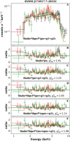 |
Fig. 1. Various spectral model fits to the spectra of 4XMM J174917.7–283329. The black, red, and green represent the spectra from the EPIC-PN, MOS1, and MOS2 detectors, respectively. Panel A represents the best-fit spectral model overlaid on the data points. The lower panels indicate the ratio plot obtained from the fitting of various models. The model components are tbabs (the Galactic absorption), tbpcf (the absorption from a medium partially covering the X-ray source), po (the power-law continuum), apec (emission from collisionally ionized diffuse gas), mcvspec (the continuum emission from the WD accretion column), g1 (the Gaussian line at 6.4 keV), and g2 (the Gaussian line at 6.7 keV). |
Next, we fitted the data with a physically motivated model called mcvspec. The model is an evolution of the model presented in Saxton et al. (2005) by Mori et al. (in prep.) and is available in XSPEC. This model represents the emission from the surface of a WD. It only includes lines produced collisionally in an ionized, diffuse gas in the accretion column of the WD. Therefore, we again added a Gaussian at 6.4 keV for the neutral iron Kα line to take the X-ray reflection of the WD surface or pre-shock region into account. While doing the fit with this model, we fixed the magnetic field, B, and the mass accretion flux, ṁ, to values of 10 MG and 5 g cm−2 s−1, respectively, which are the values typically found in IPs. The WD mass obtained by fitting this model is  .
.
3.1.2. 4XMM J174954.6–294336
The field around 4XMM J174954.6–294336 was observed twice by XMM-Newton. The observation done on 07 October 2017 (ObsID 0801681401) was performed in full frame mode. However, the source fell into the chip gap of the MOS1 detector, and therefore we report only the analysis of the EPIC-pn and MOS2 detectors. The source was also observed by XMM-Newton on 06 April 2018 (ObsID 0801683401) by all three detectors. We noticed that between the 2017 and 2018 observations, the source flux varied by a factor of 1.45. However, the shapes of the continua are very similar. Therefore, we fitted the combined spectra of the 2017 and 2018 observations to gain statistics.
Fitting an absorbed power-law model provides a best-fit photon index of Γ = 0.4 ± 0.2. Residuals around the iron line complex are clearly visible in the ratio plot, which is shown in panel B of Fig. 2. To resolve the excess in the 6–7 keV band, we added two Gaussians, at 6.4 keV and 6.7 keV, to the power-law model, which improves the fit by Δχ2 = 29 for two additional d.o.f. We performed an F test, which gives a detection significance of 99.98% and 99.86% for the 6.4 keV and 6.7 keV lines, respectively. Adding another Gaussian at 6.9 keV for the Fe XXVI line does not improve the fit. The equivalent width of the lines at 6.4 keV and 6.7 keV are  eV and
  eV, respectively. Next, we added a partial covering absorption model to the power-law continuum, which improves the fit marginally, by Δχ2 = 7, for two additional d.o.f. However, we noticed while fitting with the apec and mcvspec continuum models that adding a partial covering absorption improves the fit by Δχ2 = 42 and 44, respectively, for two extra additional d.o.f. Fitting with the apec model provides a best-fit plasma temperature of kT = 35 ± 17 keV. We also fitted the spectra with the mcvspec model. As done for 4XMM J174917.7–283329 while fitting with the mcvspec model, we fixed B to 10 MG and ṁ to 5 g cm−2 and s−1. The mass of the central compact object estimated from the mcvspec model is
  .
.
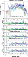 |
Fig. 2. Same as Fig. 1 but for the source 4XMM J174954.6–294336. The black, red, and green data points are from the EPIC-pn, MOS1, and MOS2 detectors of ObsID 0801683401. The blue and cyan data points are from the EPIC-pn and MOS2 detectors of ObsID 0801681401. |
3.2. Periodicity search
We computed the power spectral densities (PSDs) to search for periodicities in the 1–10 keV light curves. For our PSD analysis, we used EPIC-pn light curves only as EPIC-pn has the shortest frame time which allows us to probe a higher frequency range. Next, to refine the detected period and estimate the error, we searched for the maximum χ2 as a function of the period using the FTOOL efseach. Then we used the refined period to fold the light curve and estimate the pulsed fraction in the 1–10 keV band. The pulsed fraction was estimated by using the formula 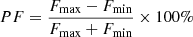 , where Fmax and Fmin are the maximum and minimum of the normalized intensity, respectively.
3.2.1. 4XMM J174917.7–283329
The left-top, middle, and bottom panels of Fig. 3 show the PSD, χ2 search, and the folded light curve of source 4XMM J174917.7–283329, respectively. The PSD shows a peak at frequency 8.39 × 10⁻⁴ Hz. We used this frequency as an input in the efsearch algorithm. The refined period and its 90% (Δχ2 = ±2.7) error is 1212 ± 3 s. We then folded the light curve with the given period, and the estimated pulsed fraction is 26 ± 6%.
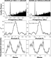 |
Fig. 3. Top panels: periodogram in Leahy normalization obtained from the EPIC-pn light curve of the sources 4XMM J174917.7–283329 (left panel) and 4XMM J174954.6–294336 (right panel). Middle panels: χ2 analysis using the FTOOL efsearch. Bottom panels: folded light curves. |
3.2.2. 4XMM J174954.6–294336
The right panels of Fig. 3 show the results obtained from the timing analysis of 4XMM J174954.6–294336 using ObsID 0801683401. The PSD shows a peak at 9.98 × 10⁻⁴ Hz. The estimated period and error from the efsearch analysis is 1002 ± 2 s. The pulsed fraction of the source is 66 ± 15%. We noticed that the eclipse duration of 2500 s at the end of the light curve introduces a spurious signal in the PSD at a frequency of 2.38 × 10⁻³ Hz. Further, we analysed the light curve from the ObsID 0801681401 and did not find any clear signal in the PSD at the corresponding frequency of the 1002 s period. In this observation, we noticed that the source light curve shows a dipping behaviour caused by absorption. Therefore, the pulsed signal is likely lost due to the variation introduced by the absorption. In fact, by computing the fast Fourier transform using the initial 10 ks of this light curve, which is unaffected by the absorption, the PSD shows two peaks, at frequencies 9.13 × 10⁻⁴ Hz, which is consistent with the 1002 s period, and 1.99 × 10⁻³ Hz, which is likely the first harmonic of the fundamental period (Fig. 4).
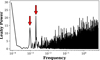 |
Fig. 4. Periodogram of 4XMM J174954.6–294336, obtained using the initial 10 ks of the observation with ObsID 0801681401. Two peaks were observed but not at a very high significance level. |
3.3. The long-term X-ray variability
We constructed a long-term light curve that spans a timescale of ten years by searching for counterparts in the Swift 2SXPS2 (Evans et al. 2020) and Chandra CSC 2.03 catalogues (Evans et al. 2010).
3.3.1. 4XMM J174917.7–283329
Figure 5 shows the long-term flux variation of the source 4XMM J174917.7–283329 (top panel). The source has been detected multiple times by XMM-Newton and Swift and displays a flux variation by a factor of six or more over the ten-year timescale.
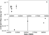 |
Fig. 5. Long-term flux variations of 4XMM J174917.7–283329 (top panel) and 4XMM J174954.6–294336 (bottom panel). Both sources show significant flux variability. |
3.3.2. 4XMM J174954.6–294336
The bottom panel of Fig. 5 shows the long-term light curve of the source 4XMM J174954.6–294336. The flux of the source varies by a factor of three. Figure 6 shows the EPIC-pn 1–10 keV, 1–4 keV, and 4–10 keV light curves. The light curves were binned with a time resolution of 500 s. They show remarkable features: a long-term variation and two eclipses near the end of the observations. Obscuration of the central X-ray source by the companion star likely causes the eclipses. In the first observation, the 1–4 keV band light curve (middle panel of Fig. 6) also shows very short-term variation associated with the absorption due to a dipping behaviour, before entering into the eclipses. During the dipping activity, the soft X-ray photons (1–4 keV) are absorbed more than the hard 4–10 keV photon, leading to an increase in the hardness ratio (bottom panel of Fig. 6); this indicates an absorption-related origin.
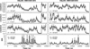 |
Fig. 6. EPIC-pn light curve of the source 4XMM J174954.6–294336 with 500 s time bins in three energy bands, 1–10 keV (top panels) and 1–4 keV, 4–10 keV (middle panels), with the hardness ratio plot shown in the bottom panels. |
4. Discussion
4.1. 4XMM J174917.7–283329
The hard X-ray spectrum of 4XMM J174917.7–283329 can be characterized by a power law with photon index Γ = 0.9 ± 0.2. The presence of excess emission in the 6–7 keV band can be attributed to the iron Kα complex. The equivalent widths of the 6.4 keV and 6.7 keV lines are  eV and
  eV, respectively. Our spectral fitting indicates the presence of an absorbing medium close to the source with NH, pcf ∼ (1.5 − 3)×1023 cm−2 that partially absorbs the incoming X-ray photons. The plasma temperature of the accreting material is
  keV. The central WD mass estimated from fitting a physical model is
  . The Galactic neutral atomic hydrogen column density towards the source is 1.1 × 1022 cm−2 (NH = NHI + NH2; Willingale et al. 2013), which is lower than the absorption column density obtained from the X-ray spectral fitting. We detected the spin period of the WD for the first time and determined it to be 1212 ± 3 s.
For better positional accuracy, we searched for an X-ray counterpart in the Chandra source catalogue; however, no Chandra observation of this region has been performed so far. Two possible Gaia counterparts were found within 0.05′ of the XMM-Newton position, with Gmag of 20.48 and 18.96. Both Gaia sources have a similar parallax of 0.48 mas, which translates to a distance of 2.08 kpc. The X-ray source flux varied by a factor of six over a timescale of ten years. The 2–10 keV luminosity variation of the source is (1–6)×1032 erg s−1.
4.2. 4XMM J174954.6–294336
The spectra of 4XMM J174954.6–294336 are characterized by a hard power law with a photon index of Γ = 0.4 ± 0.2, which is typically seen from accreting WDs. Moreover, a partially absorbed optically thin plasma of temperature kT = 35 ± 16 keV provides an adequate fit to the spectra. In addition to that, the spectra display the presence of fluorescent 6.4 keV and ionized 6.7 keV lines. The equivalent widths of the lines are  eV and
  eV for 6.4 keV and 6.7 keV, respectively. The 6.4 keV line originates from the reflection from the surface of the WD or from the pre-shock region in the accretion column and typically has an equivalent width of 150 eV (Ezuka & Ishida 1999).
The X-ray light curve shows coherent pulsations with a period of 1002 ± 2 s. The pulsation signal was suppressed in an earlier XMM-Newton observation (ObsID 0801681401). This is due to the energy-dependent absorption dips (prominent in the 1–4 keV band, middle panel of Fig. 6), which dilute the coherent pulsations. However, the pulsations were marginally detected in the initial one-third of that observation, which is unaffected by the dips. These dips are believed to be caused by photoelectric absorption by surrounding material. In the later observation, 0801683401, the dipping phenomenon is not present in the soft band 1–4 keV light curve before the source goes into the eclipse phase. This suggests the dips are highly irregular and variable from orbit to orbit. A similar dipping behaviour has also been detected in other X-ray eclipsing sources, such as dwarf novae (Mukai et al. 2009) and low-mass X-ray binaries (Díaz Trigo et al. 2006; Ponti et al. 2016). It is well established that dipping phenomena are seen in high inclination systems. The physical model for explaining this dipping behaviour is linked to the obscuration of the central X-ray source by absorbing material in the region where the stream of material from the companion star hits the outer rim of the accretion disk. This leads to the thickening of the disk rim with increasing azimuth, generating a thick bulge where the stream hits the disk edge, and the dipping occurs when the bulge intercepts the line of sight to the central X-ray source (White & Mason 1985). On the other hand, there is another physical picture of a dipping phenomena where the disk structure is fixed. The dipping activity originates from the interaction of remaining matter with the stream above and below the accretion disk (Frank et al. 1987).
The source 4XMM J174954.6–294336 is classified as a nova-like variable (Ritter & Kolb 2003). The source was detected by Chandra in the GBS and is designated as CXOGBS J174954.5–294335 (Jonker et al. 2011, 2014). Udalski et al. (2012) performed a systematic search for optical counterparts of GBS sources, and the source appeared in OGLE-IV fields. Two possible optical counterparts within 3 9 of the Chandra source position were found: a variable red giant with a period of 31.65 days with Imag = 15.67 and a fainter eclipsing binary with a period of 0.3587 days with Imag = 17.98. The Chandra and XMM-Newton source locations are consistent at a 2σ position uncertainty. The eclipsing binary system has an observed V − I color magnitude of 1.52. Britt et al. (2014) also performed an optical search for the GBS sources using the Blanco 4 m Telescope at CTIO. An optical counterpart of rmag = 19.21 was found to be associated with the X-ray source. Its optical light curve shows a periodic variability of 0.4 mag and an eclipse of almost one magnitude depth. Given the detection of the eclipses in the X-ray light curves, it is very likely that the eclipsing binary with the period of Porb = 0.3587 days is the actual optical counterpart of the X-ray source 4XMM J174954.6−294336. Johnson et al. (2017) analysed optical photometry data from DECam and OGLE. They obtained a similar orbital period as Udalski et al. (2012) and determined the spin period of the WD to be 503.3 s. The detected 1002 s X-ray periodicity is consistent with twice the optical period of 503.3 s. In a later XMM-Newton observation (ObsID 0801681401), the peaks close to 1002 and 503 s were detected in the initial 10 ks observation (Fig. 4). This indicates that the true spin period is 1002 s. Furthermore, Johnson et al. (2017) analysed the data from Chandra and detected a total X-ray eclipse. However, the Chandra data do not have a sufficiently high signal-to-noise ratio to detect the asymmetric shape of the eclipses or the iron line complex. We searched for counterparts in the Gaia catalogue (Gaia Collaboration 2016, 2023). An optical source with GaiaGmag = 18.97 is consistent in position with the eclipsing system. The estimated parallax obtained from the Gaia data is 0.61 ± 0.34 mas, which translates to a distance to the source of
  kpc.
kpc.
In each of the two XMM-Newton observations, we detected an X-ray eclipse in which the count rate went to zero. In one observation, we detected a total X-ray eclipse; however, in the later observation, only the ingress phase was caught. So far, only a few accreting WDs are known to display eclipses in X-rays (Hellier 1997; Schwope et al. 2001; Pandel et al. 2002; Ramsay & Cropper 2007; Mukai et al. 2009), and 4XMM J174954.6–294336 is only the second known IP to show complete eclipses in X-rays; the first was XY Ari (Hellier 1997). X-ray eclipses are a powerful diagnostic tool for constraining the geometry of a binary system. The duration of the eclipse ingress (the time interval between the first and second contact) and egress (the time interval between the third and fourth contact) is used to estimate the fractional area, f, of the X-ray-emitting region on the WD surface. So far, f has only been constrained for one IP (Hellier 1997). Typically, the ingress and egress times are a few seconds. The ingress phase of 4XMM J174954.6–294336 lasted around 1500 s, which is much longer than what had previously been found in eclipsing WDs. We detected one complete eclipse, which is asymmetric. The egress phase takes less than 500 s. Further, it is noticeable that the asymmetry is more pronounced in the soft 1–4 keV band than in the hard 4–10 keV band, suggesting an absorption-related origin. A similar asymmetric eclipse behaviour was seen in the eclipsing polar HU Aqr (Schwope et al. 2001) in which the ingress took longer because of the effect of absorption dips, as discussed above. At the same time, the egress is clean and lasts only 1.3 s. Asymmetric eclipses are more common in eclipsing high-mass X-ray binaries, such as 4U 1700–37 (Haberl et al. 1989) and Vela X-1 (Haberl & White 1990; Falanga et al. 2015). Falanga et al. (2015) studied a sample of bright high-mass X-ray binaries using data from INTEGRAL and find that the asymmetric shape is seen more clearly in the soft (1.3–3, 3–5, and 5–12 keV) bands than in the hard (40–150 keV) band. They suggest that the asymmetry is caused by an increase in the local absorption column density due to accretion wakes (Blondin et al. 1990; Manousakis et al. 2012). During the egress phase, the wake is located behind the compact object along the line of sight, thus not leading to any apparent increase in the local absorption column density. Therefore, the egress phase is clean and much shorter than the ingress phase. However, the companion of 4XMM J174954.6–294336 is unlikely to be a high-mass system as Johnson et al. (2017) estimated the spectral type of the donor to be G3V-G5V from the density–period relation, which is associated with a main-sequence star of 0.9 − 1.0 M⊙.
The estimated distance of 1.64 kpc to the source suggests a 2–10 keV luminosity of (1–4)×1032 erg s−1. On the other hand, the mean Galactic absorption column density towards the source location is 1.0 × 1022 cm−2 (Willingale et al. 2013), which is lower than, but within a factor of two of, the value obtained from the spectral fitting of the source.
Optical measurements of a sample of 32 sources indicate the mean WD mass among CVs is 0.83 ± 0.23 M⊙ (Zorotovic et al. 2011). On the other hand, using RXTE observations of 20 magnetic CVs, Ramsay (2000) derived a mean mass of 0.85 ± 0.21 M⊙ and 0.80 ± 0.14 M⊙ for IPs and polars, respectively. In recent years NuSTAR observations have been effective in measuring mass due to the high energy coverage and sensitivity of the instrument (Hailey et al. 2016; Suleimanov et al. 2016, 2019; Shaw et al. 2020). Shaw et al. (2020) measured the mass of 19 IPs using NuSTAR and find the mean mass to be 0.77 ± 0.10 M⊙. These studies suggest that the masses of CVs, IPs, and polars are similar to one another but higher than pre-CVs and isolated WDs, giving rise to a WD mass problem. The pre-CV population has a mean mass of 0.67 ± 0.21 M⊙ (Zorotovic et al. 2011), and isolated WDs have a mean mass of 0.53 ± 0.15 M⊙ (Kepler et al. 2016). Understanding the mass distribution of accreting WDs is crucial for explaining the formation and evolution of magnetic and non-magnetic CVs. We obtained the mass of the WDs by fitting a physical spectral model to the spectra. For both sources, the estimated mass is consistent with the mean mass of CVs. While doing the spectral fit, we fixed the B and ṁ due to degeneracy; this may have had some effect on the estimation of the mass. A few IPs in the GC and Galactic bulge regions are found to have masses above 1 M⊙, such as IGR J1807–4146 ( ; Coughenour et al. 2022), 4XMM J174033.8−301501 (
 ; Mondal et al. 2022), and CXO J174517.0–321356.5 (1.1 ± 0.1 M⊙; Vermette et al. in prep.).
5. Conclusions
In this paper we have performed detailed spectral and timing studies of two highly variable X-ray sources located within 1 5 of the GC. Furthermore, we characterized the sources using their multi-wavelength counterparts.
The 1–10 keV spectra of 4XMM J174917.7−283329 can be characterized as emission from optically thin plasma with a temperature  keV. In addition to that, a partial covering absorption with column density much higher than the Galactic value is required to fit the spectrum. The partial covering can be inferred as absorption due to circumstellar gas located close to the source. We estimate the mass of the central WD to be
  . Our timing analysis revealed pulsations with a period of 1212 ± 3 s, and the long-term flux measurements suggest the source is highly variable.
The hard X-ray spectrum of 4XMM J174954.6−294336 resembles in shape the typical spectra seen from accreting WDs. The source had already been identified as an IP with an orbital period of 0.3587 days. The X-ray spectra are well fitted by a model of optically thin plasma of kT ∼ 35 keV. The estimated mass of the WD is  . We performed a Fourier timing analysis and detected pulsations with a period of 1002 ± 2 s. The long-term observations indicate a flux variability by a factor of three. Since these types of sources are naturally variable, a flux variation of this amplitude is expected. In addition to that, the short-term X-ray light curves display complete eclipses and absorption dips. Due to the limited statistical quality of the data and the number of eclipses detected, a detailed phase-dependent study is not possible. Follow-up X-ray observations of 4XMM J174954.6–294336 with more detected eclipses will help constrain the binary system parameters. Furthermore, a detailed study of the eclipses has the potential to test the boundary layer picture of X-ray emission from accreting WDs.
Acknowledgments
SM, GP, and KA acknowledge financial support from the European Research Council (ERC) under the European Union’s Horizon 2020 research and innovation program “HotMilk” (grant agreement No. 865637). GP acknowledges support from Bando per il Finanziamento della Ricerca Fondamentale 2022 dell’Istituto Nazionale di Astrofisica (INAF): GO Large program. MRM acknowledges support from NASA under grant GO1-22138X to UCLA. NR is supported by the ERC Consolidator Grant “MAGNESIA” under grant agreement No. 817661, and also partially supported by the program Unidad de Excelencia Maria de Maetzu de Maeztu CEX2020-001058-M. The work has made use of publicly available data from HEASARC Online Service, XMM-Newton Science Analysis System (SAS) developed by the European Space Agency (ESA). Software: Python (Van Rossum & Drake 2009), Jupyter (Kluyver et al. 2016), NumPy (van der Walt et al. 2011; Harris et al. 2020), matplotlib (Hunter 2007).
References
- Aizu, K. 1973, Progr. Theoret. Phys., 49, 1184 [NASA ADS] [CrossRef] [Google Scholar]
- Arnaud, K. A. 1996, in Astronomical Data Analysis Software and Systems V, eds. G. H. Jacoby, & J. Barnes, ASP Conf. Ser., 101, 17 [NASA ADS] [Google Scholar]
- Barlow, E. J., Knigge, C., Bird, A. J., et al. 2006, MNRAS, 372, 224 [NASA ADS] [CrossRef] [Google Scholar]
- Baumgartner, W. H., Tueller, J., Markwardt, C. B., et al. 2013, ApJS, 207, 19 [Google Scholar]
- Beuermann, K., Thomas, H. C., Reinsch, K., et al. 1999, A&A, 347, 47 [NASA ADS] [Google Scholar]
- Blondin, J. M., Kallman, T. R., Fryxell, B. A., & Taam, R. E. 1990, ApJ, 356, 591 [Google Scholar]
- Britt, C. T., Hynes, R. I., Johnson, C. B., et al. 2014, ApJS, 214, 10 [NASA ADS] [CrossRef] [Google Scholar]
- Coughenour, B. M., Tomsick, J. A., Shaw, A. W., et al. 2022, MNRAS, 511, 4582 [NASA ADS] [CrossRef] [Google Scholar]
- Cropper, M. 1990, Space. Sec. Rev., 54, 195 [NASA ADS] [Google Scholar]
- Díaz Trigo, M., Parmar, A. N., Boirin, L., Méndez, M., & Kaastra, J. S. 2006, A&A, 445, 179 [NASA ADS] [CrossRef] [EDP Sciences] [Google Scholar]
- Edmonds, P. D., Gilliland, R. L., Heinke, C. O., & Grindlay, J. E. 2003a, ApJ, 596, 1177 [NASA ADS] [CrossRef] [Google Scholar]
- Edmonds, P. D., Gilliland, R. L., Heinke, C. O., & Grindlay, J. E. 2003b, ApJ, 596, 1197 [NASA ADS] [CrossRef] [Google Scholar]
- Evans, I. N., Primini, F. A., Glotfelty, K. J., et al. 2010, ApJS, 189, 37 [NASA ADS] [CrossRef] [Google Scholar]
- Evans, P. A., Page, K. L., Osborne, J. P., et al. 2020, ApJS, 247, 54 [Google Scholar]
- Ezuka, H., & Ishida, M. 1999, ApJS, 120, 277 [NASA ADS] [CrossRef] [Google Scholar]
- Falanga, M., Bozzo, E., Lutovinov, A., et al. 2015, A&A, 577, A130 [NASA ADS] [CrossRef] [EDP Sciences] [Google Scholar]
- Frank, J., King, A. R., & Lasota, J. P. 1987, A&A, 178, 137 [NASA ADS] [Google Scholar]
- Gaia Collaboration (Prusti, T., et al.) 2016, A&A, 595, A1 [NASA ADS] [CrossRef] [EDP Sciences] [Google Scholar]
- Gaia Collaboration (Vallenari, A., et al.) 2023, A&A, in press, https://doi.org/10.1051/0004-6361/202243940 [Google Scholar]
- Gosnell, N. M., Pooley, D., Geller, A. M., et al. 2012, ApJ, 745, 57 [NASA ADS] [CrossRef] [Google Scholar]
- Grindlay, J. E., Heinke, C., Edmonds, P. D., & Murray, S. S. 2001a, Science, 292, 2290 [NASA ADS] [CrossRef] [Google Scholar]
- Grindlay, J. E., Heinke, C. O., Edmonds, P. D., Murray, S. S., & Cool, A. M. 2001b, ApJ, 563, L53 [NASA ADS] [CrossRef] [Google Scholar]
- Haberl, F., & White, N. E. 1990, ApJ, 361, 225 [Google Scholar]
- Haberl, F., White, N. E., & Kallman, T. R. 1989, ApJ, 343, 409 [NASA ADS] [CrossRef] [Google Scholar]
- Hailey, C. J., Mori, K., Perez, K., et al. 2016, ApJ, 826, 160 [NASA ADS] [CrossRef] [Google Scholar]
- Harris, C. R., Millman, K. J., van der Walt, S. J., et al. 2020, Nature, 585, 357 [NASA ADS] [CrossRef] [Google Scholar]
- Hellier, C. 1997, MNRAS, 291, 71 [NASA ADS] [Google Scholar]
- Hong, J. 2012, MNRAS, 427, 1633 [NASA ADS] [CrossRef] [Google Scholar]
- Hong, J. S., van den Berg, M., Grindlay, J. E., & Laycock, S. 2009, ApJ, 706, 223 [NASA ADS] [CrossRef] [Google Scholar]
- Hunter, J. D. 2007, Comput. Sci. Eng., 9, 90 [NASA ADS] [CrossRef] [Google Scholar]
- Jansen, F., Lumb, D., Altieri, B., et al. 2001, A&A, 365, L1 [NASA ADS] [CrossRef] [EDP Sciences] [Google Scholar]
- Johnson, C. B., Torres, M. A. P., Hynes, R. I., et al. 2017, MNRAS, 466, 129 [NASA ADS] [CrossRef] [Google Scholar]
- Jonker, P. G., Bassa, C. G., Nelemans, G., et al. 2011, ApJS, 194, 18 [NASA ADS] [CrossRef] [Google Scholar]
- Jonker, P. G., Torres, M. A. P., Hynes, R. I., et al. 2014, ApJS, 210, 18 [NASA ADS] [CrossRef] [Google Scholar]
- Kepler, S. O., Pelisoli, I., Koester, D., et al. 2016, MNRAS, 455, 3413 [NASA ADS] [CrossRef] [Google Scholar]
- Kluyver, T., Ragan-Kelley, B., Pérez, F., et al. 2016, in Positioning and Power in Academic Publishing: Players, Agents and Agendas, eds. F. Loizides, & B. Schmidt (IOS Press), 87 [Google Scholar]
- Krivonos, R., Revnivtsev, M., Churazov, E., et al. 2007, A&A, 463, 957 [NASA ADS] [CrossRef] [EDP Sciences] [Google Scholar]
- Manousakis, A., Walter, R., & Blondin, J. M. 2012, A&A, 547, A20 [NASA ADS] [CrossRef] [EDP Sciences] [Google Scholar]
- Meliani, M. T., de Araujo, J. C. N., & Aguiar, O. D. 2000, A&A, 358, 417 [NASA ADS] [Google Scholar]
- Mondal, S., Ponti, G., Haberl, F., et al. 2022, A&A, 666, A150 [NASA ADS] [CrossRef] [EDP Sciences] [Google Scholar]
- Mukai, K. 2017, PASP, 129, 062001 [Google Scholar]
- Mukai, K., Zietsman, E., & Still, M. 2009, ApJ, 707, 652 [NASA ADS] [CrossRef] [Google Scholar]
- Muno, M. P., Baganoff, F. K., Bautz, M. W., et al. 2003, ApJ, 589, 225 [NASA ADS] [CrossRef] [Google Scholar]
- Pandel, D., Cordova, F. A., Shirey, R. E., et al. 2002, MNRAS, 332, 116 [NASA ADS] [CrossRef] [Google Scholar]
- Patterson, J. 1994, PASP, 106, 209 [Google Scholar]
- Perez, K., Hailey, C. J., Bauer, F. E., et al. 2015, Nature, 520, 646 [NASA ADS] [CrossRef] [Google Scholar]
- Ponti, G., Morris, M. R., Terrier, R., & Goldwurm, A. 2013, in Cosmic Rays in Star-Forming Environments, eds. D. F. Torres, & O. Reimer, Astrophys. Space Sci. Proc., 34, 331 [NASA ADS] [CrossRef] [Google Scholar]
- Ponti, G., Morris, M. R., Terrier, R., et al. 2015, MNRAS, 453, 172 [Google Scholar]
- Ponti, G., Bianchi, S., Muñoz-Darias, T., et al. 2016, Astron. Nachr., 337, 512 [Google Scholar]
- Ponti, G., Hofmann, F., Churazov, E., et al. 2019, Nature, 567, 347 [Google Scholar]
- Pretorius, M. L., Knigge, C., O’Donoghue, D., et al. 2007, MNRAS, 382, 1279 [CrossRef] [Google Scholar]
- Ramsay, G. 2000, MNRAS, 314, 403 [NASA ADS] [CrossRef] [Google Scholar]
- Ramsay, G., & Cropper, M. 2007, MNRAS, 379, 1209 [NASA ADS] [CrossRef] [Google Scholar]
- Revnivtsev, M., Sazonov, S., Churazov, E., et al. 2009, Nature, 458, 1142 [Google Scholar]
- Ritter, H., & Kolb, U. 2003, A&A, 404, 301 [NASA ADS] [CrossRef] [EDP Sciences] [Google Scholar]
- Saxton, C. J., Wu, K., Cropper, M., & Ramsay, G. 2005, MNRAS, 360, 1091 [NASA ADS] [CrossRef] [Google Scholar]
- Schwope, A. D., Schwarz, R., Sirk, M., & Howell, S. B. 2001, A&A, 375, 419 [NASA ADS] [CrossRef] [EDP Sciences] [Google Scholar]
- Shaw, A. W., Heinke, C. O., Mukai, K., et al. 2020, MNRAS, 498, 3457 [NASA ADS] [CrossRef] [Google Scholar]
- Suleimanov, V., Doroshenko, V., Ducci, L., Zhukov, G. V., & Werner, K. 2016, A&A, 591, A35 [NASA ADS] [CrossRef] [EDP Sciences] [Google Scholar]
- Suleimanov, V. F., Doroshenko, V., & Werner, K. 2019, MNRAS, 482, 3622 [NASA ADS] [CrossRef] [Google Scholar]
- Udalski, A., Kowalczyk, K., Soszyński, I., et al. 2012, Acta Astron., 62, 133 [NASA ADS] [Google Scholar]
- van der Walt, S., Colbert, S. C., & Varoquaux, G. 2011, Comput. Sci. Eng., 13, 22 [Google Scholar]
- Van Rossum, G., & Drake, F. L. 2009, Python 3 Reference Manual (Scotts Valley: CreateSpace) [Google Scholar]
- Warwick, R. S., Turner, M. J. L., Watson, M. G., & Willingale, R. 1985, Nature, 317, 218 [NASA ADS] [CrossRef] [Google Scholar]
- Webb, N. A., Coriat, M., Traulsen, I., et al. 2020, A&A, 641, A136 [NASA ADS] [CrossRef] [EDP Sciences] [Google Scholar]
- White, N. E., & Mason, K. O. 1985, Space. Sec. Rev., 40, 167 [NASA ADS] [CrossRef] [Google Scholar]
- Willingale, R., Starling, R. L. C., Beardmore, A. P., Tanvir, N. R., & O’Brien, P. T. 2013, MNRAS, 431, 394 [Google Scholar]
- Wilms, J., Allen, A., & McCray, R. 2000, ApJ, 542, 914 [Google Scholar]
- Yamauchi, S., Nobukawa, K. K., Nobukawa, M., Uchiyama, H., & Koyama, K. 2016, PASJ, 68, 59 [NASA ADS] [CrossRef] [Google Scholar]
- Yuasa, T., Makishima, K., & Nakazawa, K. 2012, ApJ, 753, 129 [NASA ADS] [CrossRef] [Google Scholar]
- Zorotovic, M., Schreiber, M. R., & Gänsicke, B. T. 2011, A&A, 536, A42 [NASA ADS] [CrossRef] [EDP Sciences] [Google Scholar]
- Zou, Z.-C., Zhou, X.-L., & Huang, Y.-F. 2020, RAA, 20, 137 [NASA ADS] [Google Scholar]
All Tables
All Figures
|
Fig. 1. Various spectral model fits to the spectra of 4XMM J174917.7–283329. The black, red, and green represent the spectra from the EPIC-PN, MOS1, and MOS2 detectors, respectively. Panel A represents the best-fit spectral model overlaid on the data points. The lower panels indicate the ratio plot obtained from the fitting of various models. The model components are tbabs (the Galactic absorption), tbpcf (the absorption from a medium partially covering the X-ray source), po (the power-law continuum), apec (emission from collisionally ionized diffuse gas), mcvspec (the continuum emission from the WD accretion column), g1 (the Gaussian line at 6.4 keV), and g2 (the Gaussian line at 6.7 keV). |
| In the text | |
|
Fig. 2. Same as Fig. 1 but for the source 4XMM J174954.6–294336. The black, red, and green data points are from the EPIC-pn, MOS1, and MOS2 detectors of ObsID 0801683401. The blue and cyan data points are from the EPIC-pn and MOS2 detectors of ObsID 0801681401. |
| In the text | |
|
Fig. 3. Top panels: periodogram in Leahy normalization obtained from the EPIC-pn light curve of the sources 4XMM J174917.7–283329 (left panel) and 4XMM J174954.6–294336 (right panel). Middle panels: χ2 analysis using the FTOOL efsearch. Bottom panels: folded light curves. |
| In the text | |
|
Fig. 4. Periodogram of 4XMM J174954.6–294336, obtained using the initial 10 ks of the observation with ObsID 0801681401. Two peaks were observed but not at a very high significance level. |
| In the text | |
|
Fig. 5. Long-term flux variations of 4XMM J174917.7–283329 (top panel) and 4XMM J174954.6–294336 (bottom panel). Both sources show significant flux variability. |
| In the text | |
|
Fig. 6. EPIC-pn light curve of the source 4XMM J174954.6–294336 with 500 s time bins in three energy bands, 1–10 keV (top panels) and 1–4 keV, 4–10 keV (middle panels), with the hardness ratio plot shown in the bottom panels. |
| In the text | |
Current usage metrics show cumulative count of Article Views (full-text article views including HTML views, PDF and ePub downloads, according to the available data) and Abstracts Views on Vision4Press platform.
Data correspond to usage on the plateform after 2015. The current usage metrics is available 48-96 hours after online publication and is updated daily on week days.
Initial download of the metrics may take a while.