| Issue |
A&A
Volume 650, June 2021
|
|
|---|---|---|
| Article Number | A138 | |
| Number of page(s) | 19 | |
| Section | Stellar structure and evolution | |
| DOI | https://doi.org/10.1051/0004-6361/202040098 | |
| Published online | 22 June 2021 | |
Activity of TRAPPIST–1 analog stars observed with TESS⋆
1
Konkoly Observatory, Research Centre for Astronomy and Earth Sciences, Konkoly Thege M. út 15-17, Budapest 1121, Hungary
e-mail: This email address is being protected from spambots. You need JavaScript enabled to view it.
2
Eötvös University, Department of Astronomy, Pf. 32, 1518 Budapest, Hungary
Received:
9
December
2020
Accepted:
23
March
2021
Abstract
As more exoplanets are being discovered around ultracool dwarfs, understanding their magnetic activity and the implications for habitability is of prime importance. To find stellar flares and photometric signatures related to starspots, continuous monitoring is necessary, which can be achieved with spaceborne observatories such as the Transiting Exoplanet Survey Satellite (TESS). We present an analysis of TRAPPIST–1 analog ultracool dwarfs with TESS full-frame image photometry from the first two years of the primary mission. A volume-limited sample up to 50 pc is constructed consisting of 339 stars closer than 0.m5 to TRAPPIST–1 on the Gaia color–magnitude diagram. We analyzed the 30 min cadence TESS light curves of 248 stars, searching for flares and rotational modulation caused by starspots. The composite flare frequency distribution of the 94 identified flares shows a power-law index that is similar to TRAPPIST–1 and contains flares up to ETESS = 3 × 1033 erg. Rotational periods shorter than 5d were determined for 42 stars, sampling the regime of fast rotators. The ages of 88 stars from the sample were estimated using kinematic information. A weak correlation between rotational period and age is observed, which is consistent with magnetic braking.
Key words: stars: activity / stars: flare / stars: late-type / stars: low-mass / starspots / stars: statistics
Full Table 2 and the individual TESS light curves are only available at the CDS via anonymous ftp to cdsarc.u-strasbg.fr (130.79.128.5) or via http://cdsarc.u-strasbg.fr/viz-bin/cat/J/A+A/650/A138
© ESO 2021
1. Introduction
Low-mass, cool M dwarfs are the prime targets when searching for exoplanets. One appealing trait of these objects is that their habitable zone is much closer to an M-dwarf host than to a solar-like star, thus detecting a possibly habitable Earth-like planet is easier. Currently there are about 4000 known exoplanets, but interestingly only very few of these were found around ultracool dwarfs (UCDs), which include late M dwarfs and brown dwarfs. One of these is Proxima Centauri (M5.5 V), the closest star to the Sun, which hosts an Earth-mass planet in its habitable zone (Anglada-Escudé et al. 2016). The other is Teegarden’s star (2MASS J02530084+1652532; M7V), where Zechmeister et al. (2019) recently reported two Earth-mass planets, which are among the lowest-mass planets discovered so far. The third example is TRAPPIST-1 (2MASS J23062928-0502285; Gaia DR2 2635476908753563008; M8V). This system is known to host seven transiting exoplanets, three of which have equilibrium temperatures that make the existence of liquid water on their surface possible (Gillon et al. 2017). However, owing to the low luminosity of these objects in the optical regime, obtaining high signal-to-noise photometric or spectroscopic observation is challenging, hence the low number of currently known exoplanets around UCDs.
The habitability of the planets hosted by UCDs is the focus of intense debates because a large fraction of these stars are magnetically active, producing frequent flares, for instance. These can damage the atmospheres of the orbiting planets by changing the atmospheric composition or completely eroding the atmosphere over time (see Vida et al. 2017, 2019b; Roettenbacher & Kane 2017; Glazier et al. 2020; Chen et al. 2021, and references therein). On the other hand these events can be the source of the UV radiation needed for abiogenesis (Ranjan et al. 2017). On our Sun a large fraction of the flares are accompanied by coronal mass ejections (CMEs), which also can have deleterious effects on planetary atmospheres. However, observations suggest that while the detected CMEs are more frequent on the later-type, more active UCDs, most of these events are unsuccessful eruptions and have velocities below the escape velocity (Vida et al. 2016, 2019a). This is further confirmed by magnetohydrodynamic simulations, which suggest that only the largest eruptions might be able to escape from the strong magnetic field of these stars (Alvarado-Gómez et al. 2018).
To understand these systems, long-term observations would be optimal. However, in this paper we chose a different approach. Instead of observing a single target for an extended period of time, we aim to gain statistical knowledge of the flaring activity based on the photometry of many similar stars. To this end, we choose TRAPPIST–1 as the main target and compile a list of similar objects we call TRAPPIST–1 analogs. As a measure of similarity we simply use the distance between stars on the Gaia color–magnitude diagram, and adopt a lower limit on parallax to have a volume-limited sample. As for the photometric observation, we use data provided by the Transiting Exoplanet Survey Satellite mission (TESS; Ricker et al. 2015). The primary mission of TESS was performed between July 2018 and July 2020, covering the majority of the sky divided into observation runs called sectors. One sector covers 24 × 96 degrees in a nearly continuous field of view (FoV), assembled from the 24 × 24 degree FoVs of four individual identical cameras lined up to provide the final geometry. The two years of the primary mission were divided into a southern survey (first year) and northern survey (second year), in which each of the corresponding 2 × 13 sectors were observed for approximately one sidereal month (∼27.3d). The sectors were arranged in a way to provide overlaps and therefore nearly continuous observations for a year at the vicinity of the ecliptic poles1. The TESS images are available for the entire FoV with a 30 min cadence, while a limited number of stars are observed with a 2 min cadence. To make our analysis homogeneous, we only use the 30 min full-frame images (FFIs). These FFIs are available for roughly three-quarters of virtually any spatially homogeneous stellar sample in the two years of the TESS primary mission, which avoids the ecliptic. Our primary objective is to detect the rare high-energy flares and many studies have shown that it is possible with this relatively long cadence (see, e.g., Davenport 2016; Van Doorsselaere et al. 2017). This cadence is also sufficient for the detection of photometric rotational period of UCDs on the order of a few days.
The structure of the paper is as follows: We define the TRAPPIST–1 analog sample in Sect. 2, then in Sect. 3 the analysis of the TESS light curves is presented, including period search and flare identification. In this section we also look for Hα emission in publicly available optical spectra and compile the approximate ages of stars in the sample. In Sect. 4, we then discuss the implications of our findings regarding the period distribution, flare rate and possible correlations. Finally the main results are summarised in Sect. 5.
2. Sample selection
Since TRAPPIST–1 lies near the ecliptic, TESS did not observe it in the first two years of the primary mission, and the next opportunity will be during the fourth year, when Sectors 42–46 will be centered on the ecliptic. So to study UCDs such as TRAPPIST–1, we selected similar stars (henceforth TRAPPIST–1 analogs) based on simple photometric criteria. The selected stars need to be closer than  to TRAPPIST–1 on the Gaia (GBP − GRP) – MG diagram (see Fig. 1). This results in a circle around TRAPPIST–1, which has the following parameters:
  ,
,  . To get a volume-limited sample for homogeneous analysis, only stars closer than 50 pc were considered. Limiting our search to nearby stars was also a practical consideration so our sample contains only targets within the reach of TESS. According to TICgen2, TRAPPIST–1 at 50 pc would be ∼17m in the TESS bandpass with photometric error around
  on 30 min exposures, which are sufficient to detect the highest-energy flares. This value agrees with the pure Gaia DR2-based estimation of
  . Such an estimation is rather accurate owing to the nearly perfect overlap of the bandpasses of the TESS cameras and Gaia GRP color (see Fig. 3 in Jordi et al. 2010).
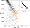 |
Fig. 1. Selection criteria on the Gaia color–magnitude diagram. The red point shows the position of TRAPPIST–1 and the orange points represent the final TRAPPIST–1 analog sample. The empty orange circles indicate stars that were not initially included as a result of the Gaia quality cuts, but were later added from existing UCD catalogs. |
We used a custom query (Table 1) on the Gaia TAP (Table Access Protocol) server3 to obtain the set of stars with reliable observations within 50 pc. The flux error limits employed in this query were based on the work of Reylé (2018). The last line of the query corresponds to the renormalised unit weight error (RUWE), retaining sources with well-behaved astrometric solutions. Since the stars of interest are in the solar neighborhood, reddening and interstellar extinction were not taken into account.
SQL query used to select the sources from the Gaia DR2 catalog using the services provided by the Gaia TAP server.
After applying our photometric criteria on this list, 271 stars remained; there were 144 also present in the UCD catalog of Reylé (2018). To complement this list with known UCDs because, for example, TRAPPIST–1 itself was excluded by RUWE, we also added stars from the List of M6-M9 Dwarfs4 curated by J. Gagné; disregarding the quality criteria used in the previous Gaia query. Also we included 36 new stars from the volume-limited Ultracool SpeXtroscopic Survey of Bardalez Gagliuffi et al. (2019) in the same manner. All the added stars are within 50 pc and inside the  circle on the Gaia color–magnitude diagram. Their exclusion from the original sample was owing to either visibility_periods_used ≤8 or RUWE. The final sample consists of 339 targets, which are summarised in Table 2. Propagating the Gaia uncertainties of TRAPPIST–1 to the selection, the scatter in the sample size is ±39. As a sanity check we queried the Simbad database with the Gaia DR2 identifiers and ∼90% of the valid spectral types were between M7 and M9. We note that while the Gaia EDR3 is now available, it could add only a few UCD candidates to the sample. According to Gaia Collaboration (2021), the number of new UCDs up to 100 pc is 1016 objects, most of which are in the faint regime that cannot be reliably observed with TESS.
TRAPPIST–1 analog sample.
The brightness distribution of our sample can be seen in Fig. 2. Since the Gaia GRP bandpass is similar to the TESS bandpass, we expect most targets to be brighter than T = 17m. Figure 3 shows the position of the targets with equal-area Aitoff projection. The open circles indicate stars that were not observed in the TESS primary mission, mostly owing to the exclusion of the ecliptic.
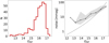 |
Fig. 2. Photometric properties of the sample. Left: brightness distribution of the final sample. Right: noise properties of the sample. The black curve shows the photometric scatter measured on the final processed light curves. The region between the 16th and 84th percentiles is shown in grey. The dashed line is the predicted noise value from TICgen. |
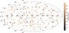 |
Fig. 3. Position of the selected stars on the sky with equatorial coordinates, color coded with distance. The stars plotted with filled points have been observed by TESS up to Sector 26. The red circle represents TRAPPIST–1. The ecliptic is shown with a dashed line for reference. |
The TESS Input Catalog (TICv8, Stassun et al. 2019) contained 325 stars from the sample with the following median parameters: log g = 5.27 ± 0.01, M = 0.092 ± 0.003 M⊙, L = 0.0007 ± 0.0004 L⊙, R = 0.116 ± 0.003 R⊙. While there are no effective temperature measurements below 2700 K in TICv8, there is a generally good agreement of the other parameters compared to Gonzales et al. (2019). Of the stars in the sample, 70 stars have temperature measurements in Gaia DR2, with a 3318 ± 23 K median value, while TRAPPIST–1 itself has  K. However, the Gaia temperatures are not reliable in this regime because the algorithm was trained on stars hotter than 3000 K and there is a degeneracy between temperature, extinction and reddening (Gaia Collaboration 2018).
3. Methods
3.1. TESS full-frame image photometry
We used all 26 sectors from the TESS primary mission, which covered ∼75% of the sky. Of the 339 objects in the sample, 248 stars (73%) were observed in at least one sector, resulting in 370 individual light curves. The FFIs were acquired with a 30 min cadence during the primary mission and the calibrated imaging data were downloaded from the MAST bulk download portal5. Starting from Sector 27, the TESS FFIs are downlinked with a 10 min cadence, providing better time resolution at the expense of larger photometric noise. To make the analysis homogeneous we only use Sectors 1–26 in this work, but the data from the extended mission will provide an interesting comparison that might be addressed in a future work.
For the extraction of light curves from a series of FFI stamps, we used a flux extraction method based on convolution-aided differential photometry named QDLP-EXTRACT, which was implemented atop the tasks of the FITSH package (Pál 2012). We used apertures with 1.5 pixel radius and an annulus from 5 to 10 pixels from the target as background to estimate the fluxes and their respective uncertainties. Since most of our targets are faint and lie in dense regions on the sky, the raw TESS light curves often contain astrophysical signals that are originated from brighter stars. To mitigate this contamination, we employed a technique based on principal component analysis (PCA) to remove instrumental and astrophysical systematics from the light curves, similar to the method used by Petralia & Micela (2020). There are also cotrending basis vectors provided by TESS (for each sector and each camera), but we chose to do PCA locally, using light curves extracted with the same method as the target, to have a homogeneous basis. Around each of our targets we selected multiple stars (up to 20) and extracted their light curves as well. Then by running PCA on these datasets, the light curve of the target could be rebuilt from several PCA components containing the variation of the nearby stars. Finally, by subtracting the PCA reconstruction from the raw light curve we could in theory remove the systematics.
The median proper motion of the sample is  , which is small compared to the 21″ pixel size of TESS. Nevertheless, we corrected the coordinates of the targets for the four-year difference between the Gaia and TESS observations. This correction was larger than 1 TESS pixel for only six targets.
To find the possible contaminating stars, we queried Gaia DR2 around our targets with 5′ radius. We corrected the position of all stars for proper motion except for stars with fewer than five astrometric parameters solved (i.e., with astrometric_params_solved ≠31). We selected the stars closer than 3′ and at most  fainter than the target (
 ). We also added stars at least 2m brighter than the target up to 5′. From this list, the brightest 20 stars were kept, leaving out objects closer than
  (∼1.5 TESS pixel) to each other and leaving out stars closer than
  to the target itself. An example of such a selection can be seen in Fig. 4, while Fig. 5 shows the extracted light curves for the selected stars around the same target.
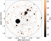 |
Fig. 4. Field of view of a selected target (Gaia DR2 2883680659313632896) from Gaia, with 173 stars brighter than 20m. The red cross denotes the target, dashed circles show the aperture and annulus used for the TESS photometry, and solid circles show the stars selected for PCA. The grid in the background illustrates the pixel scale of TESS. |
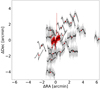 |
Fig. 5. Extracted light curves from the circular apertures of Fig. 4, with red dots indicating the celestial position of the sources. Some common trends can be identified, while the large flare seen on the target (red curve) does not seem to appear anywhere else. |
As a post-processing of the light curves, we removed bad photometric points with quality flags masked with the bitmask 10101111 (manual exclude, reaction wheel desaturation, Earth pointing, coarse pointing, safe mode, or attitude tweak; see also Tenenbaum & Jenkins 2018) as well as 1% of the points with the largest error bars on the given light curve. We also removed NaN values that were possibly due to zero measured flux or instrumental errors. Then the light curves of the nearby stars used for PCA were interpolated to the time values of the main target, so that all datasets contain the same number of points. We also tried the same approach with flux instead of magnitude, but the results were essentially the same. A light curve containing periodic variation and a flare event can be seen in Fig. 6.
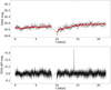 |
Fig. 6. PCA reconstruction of the light curve from Fig. 5. The black points in the upper panel show the light curve created by QDLP_EXTRACT; the red curve shows the PCA reconstruction. The corrected light curve can be seen in the lower panel, showing a dominant flare and periodic variation. |
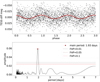 |
Fig. 7. Period analysis for the corrected light curve from Fig. 6. Upper panel: light curve phase folded with the 1.93d period, which can be identified on the Lomb–Scargle periodogram below. |
3.2. Period search
Ultracool dwarfs often have rotational periods of less than a few days, therefore even one 27d long TESS sector could be enough to detect the rotational modulation caused by starspots. To search for rotational periods, we inspected the Lomb–Scargle periodogram (Lomb 1976; Scargle 1982) of all stars in the observed sample (248 stars out of 339, with 370 light curves). To make the analysis homogeneous, the periodograms were plotted separately for each sector and only periods shorter than 5d were considered (similar to Medina et al. 2020 or Günther et al. 2020). Several targets showed Lomb–Scargle peaks longer than 5d, but the strong contamination and short temporal baseline would make these detections ambiguous.
After clipping the outliers from the light curve with 3σ threshold, the Lomb–Scargle periodogram was plotted and the five largest peaks were identified between 1.5 h and 5d. We folded the light curves with these trial periods and inspected the results manually. Since all the stars with detected period showed simple sinusoidal variation, only one Fourier term was used for the analysis.
To assess the significance of the periodogram peaks, the false alarm probability (FAP) was calculated. The FAP quantifies the probability that a peak with the given height is observed from Gaussian noise alone, purely by chance. We note that a FAP value close to zero does not mean that the given period is the correct one. Only peaks with FAP less than 1% were considered.
To calculate the uncertainty of the peak position, we took the best-fitting sinusoidal model and created 1000 realizations adding Gaussian noise with the scatter of the residual light curve. The period analysis was repeated and the position of the largest peak was saved. The uncertainty of the period was then calculated as the standard deviation of these periods. We note that this uncertainty generally scales with the value of the period itself, increasing for longer periods.
Most of the stars with detected period show simple sinusoidal light curves, possibly as a consequence of the relatively long cadence compared to the short rotational periods. If these stars would show complex rotational modulation (e.g., as in Zhan et al. 2019), the 30 min integration time would blur the sharp features. The distribution of the detected rotational periods is plotted in Fig. 8. We discuss this again in Sect. 4.
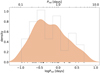 |
Fig. 8. Rotational period distribution of the sample with TESS. The one-dimensional kernel density estimation plotted with orange is calculated with a Gaussian kernel with bandwidth of 0.15. The black ticks show the individual period values. Only periods below 5d were kept owing to the 27d baseline of TESS sectors. |
3.3. Flares
Flares appear as a sudden brightening of the stellar atmosphere, which occurs when the magnetic field lines reconnect and a portion of magnetic energy is released. Their usual timescale is minutes to hours. Even though white-light flares are rarely observed on the Sun, they are quite common on later-type stars (see, e.g., Namekata et al. 2017). Apart from the rotational modulation caused by starspots, flares are the most easily observable manifestation of magnetic activity in optical light curves. So to characterize the activity of TRAPPIST–1 analogs, we searched for flares on the 30 min TESS light curves.
As a result of the high noise level of the light curves, we chose to identify flares manually. We selected events with at least two consecutive outlying points (with at least one point exceeding twice the local scatter), resulting in 94 detections. These flares were found on 21 stars, all of which had a detected rotational period; this means that 50% of the fast rotators in our sample show flares (similar to the ∼60% found by Günther et al. 2020).
To characterize the flares, we calculated the equivalent duration (ED, Gershberg 1972), that is, the integrated area under the flare curve; this is the time needed for the quiescent star to radiate the same amount of energy that was released during the flare event. The total energy output of an event can be calculated by multiplying this value with the quiescent luminosity of the star. We converted the light curves to flux and ran the full detrending procedure, which involves normalising by the median value, and then subtracting the PCA reconstruction, resulting in dimensionless flux centered on zero. We then iteratively σ-clipped points with lower and upper rejection threshold of 3σ and 2σ, respectively, which effectively removed the flares. We then smoothed the remaining dataset using a LOWESS filter (locally weighted linear regression, Cleveland 1979) with a Gaussian kernel width of 0.06d. This smoothed dataset was then interpolated onto the time frame of the original light curve and subtracted from it. This step removed the variation induced by starspots. We calculated the ED on these light curves employing two different approaches. First, we simply integrated the area of the flares using the trapezoidal rule. To estimate the uncertainty of this method, we re-sampled the light curve using the flux values and error bars as the mean and scatter of a Gaussian distribution. We generated 1000 such realizations of the light curve, calculated the ED again, and took the standard deviation.
As a second approach, we fitted the flares with the single-peaked empirical template of Davenport et al. (2014), parameterized by the tpeak time of the peak, A amplitude and t1/2 width of the flare. After transforming the measured time t to  , the flare template function is given by
 (1)
(1)
To fit the observations we used the Markov chain Monte Carlo (MCMC) implementation of PYMC (Fonnesbeck et al. 2015) with uniform prior around an approximate tguess on tpeak, and exponential priors on A and t1/2, where λ is the parameter of the exponential distribution as follows:
 (2)
(2)
 (3)
(3)
 (4)
(4)
We ran the MCMC chains starting from the maximum a posteriori value for 100 000 steps, discarding the first 20 000 steps as burn-in and only leaving every second step as thinning. A successful fit can be seen in Fig. 9 (following the example of Fig. 6), while for a few smaller flares the MCMC chain did not converge (13 of the 94 flare events, see Table B.1). The fits generally overestimated the flare amplitudes (see Fig. 10), and hence the EDs, but they give a reliable estimate of t1/2 even for shorter events. A similar behavior is observed by Raetz et al. (2020), where the amplitudes are systematically higher using a Kepler short cadence light curve compared to a long cadence light curve. We experimented with fitting only two parameters, after forcing the fitted ED to be equal to the previously calculated ED, but essentially the same behavior was observed. According to Fig. 11, the flare EDs mainly scale with the amplitude and there is no dependence on t1/2.
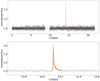 |
Fig. 9. Flare event fitted with the analytical template following the example of Fig. 6. The summed ED is 15.4 ± 2.9 min, while the fit gives 12.9 ± 4.4 min. |
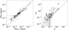 |
Fig. 10. Flare parameters from different methods. Left: comparison of the summed and fitted EDs. While they generally give the same result, they can differ by a factor of 2–3. Right: comparison of the observed flare amplitude (the highest flux value) and the fitted amplitude. Owing to the low time resolution, the observed peak is generally smaller. |
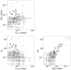 |
Fig. 11. Correlations between the flare parameters. |
The ED of the 94 flare events were converted to energy by multiplying by the quiescent stellar luminosity. Since the sample consists of stars similar to TRAPPIST–1, we simply used the luminosity of this object for all targets. This value was calculated by convolving the TESS response function6 with a BT-NextGen model spectrum (Teff = 2600 K, log g = 5.0, [Fe/H] = 0), scaling with the Lbol = 0.00061 ± 0.00002 L⊙ bolometric luminosity of TRAPPIST–1 from Gonzales et al. (2019). The estimated luminosity of TRAPPIST–1 in the TESS bandpass is thus LTESS = (2.1 ± 0.3)×1029 erg s−1; the nominal uncertainty was calculated using models with ±100 K temperature. Using a simple blackbody spectrum with the same temperature would give 2.9 × 1029 erg s−1. Integrating the same BT-NextGen model spectrum gives LKepler = (5.6 ± 1.5)×1028 erg s−1 for the luminosity in the Kepler bandpass. Compared to the nominal errors cited, the dominating source of uncertainty is the different luminosities within the sample itself, since MG varies by  .
.
As a validation for the temperature and luminosity used above, Gonzales et al. (2019) lists four field dwarfs similar to TRAPPIST–1, with 2603 K and 0.00058 L⊙ mean temperature and luminosity in their Table 3 and plotted in their Fig. 2a. These four stars are also present in our sample, and LHS 132 (Gaia DR2 4989399774745144448) and LHS 3003 (Gaia DR2 6224387727748521344) have already been observed by TESS.
3.3.1. Feasibility check with downgraded Kepler K2 data
To demonstrate the viability of this project, we converted real photometric observations of TRAPPIST–1 to match the quality of a TESS FFI dataset. We took the Kepler K2 short cadence light curve of Vida et al. (2017), converted it from magnitude to flux, scaled up the noise level by a factor of 10 (ratio of the Kepler and TESS apertures), and rebinned it from a 1 to 30 min cadence. We then inspected the resulting light curve (Fig. 12) and identified flare events passing the same criteria as the TRAPPIST–1 analogs. While the original light curve showed 42 distinguishable flares, from the downgraded light curve we could only identify eight of them, comprise of only those with the highest energies. However, the energy estimates agreed within the nominal uncertainties. We note that some of the larger flares remained as a single outlier point, but in real observations we could not safely label such events as flares, so we omitted these. It appears that flares with energies above ∼1031 erg can be observed even with the 10 cm aperture of TESS on a T ∼ 14m star.
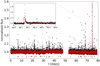 |
Fig. 12. Kepler K2 light curve of TRAPPIST–1 from Vida et al. (2017) (black) rebinned to 30 min time resolution and with TESS-like scatter (red). The black and red ticks below the light curve indicate the position of flares found in the corresponding dataset. |
3.3.2. Completeness
Less energetic flares are harder to distinguish from noise, so they are easily missed. To de-bias the flare frequency distribution (FFD) from this selection effect, we calculate the flare recovery rate (hereafter called completeness) for each light curve, for given flare energies. To do this, we inject artificial flare signals into the light curves and try to recover them.
Each of the light curves were converted to flux and clipped with a 3σ threshold. The clipped values were then linearly interpolated to fill the gaps induced by real flare events. Next, we added artificial flares with different EDs. To generate a flare with the given ED, tpeak was drawn from the observed time interval, t1/2 was drawn uniformly from 0.001d to 0.05d, and the amplitude of the flare was scaled to match the required ED. Next, the local scatter was calculated in a 4d long interval and the light curve was smoothed with a 0.2d wide LOWESS kernel. A flare is considered to be detected if a point is twice the scatter above the smoothed light curve and the following point still exceeds once the scatter. This criterion was chosen to match visual inspection. For each light curve, 100 ED bins were defined logarithmically from 10 to 104 s and 100 random flares were generated for each ED. The completeness is defined as the fraction of recovered flares.
Taking the multiplicative inverse of the completeness value for each detected flare energy, the FFD calculated from a single light curve can be corrected. However, most of the flares in our sample come from different stars with different photometric noise properties, that is, with different completeness curves. In order to correct the composite FFD of the whole sample, a single representative correction curve is needed. For this purpose we simply average the completeness curves calculated from each individual light curve. As shown Fig. 13, this approach is equivalent to a completeness curve calculated from all the light curves concatenated into a single dataset spanning ∼23 years. The uncertainty is calculated from the 84th and 16th percentiles of all the single-sector completeness curves. We note that for lower energies even a small difference in the recovery rate can result in a large difference in the composite FFD, thus the lower energy part should be treated with caution. Normally, when a similar approach is used, the difference between the original and corrected FFD is only a few percent. We also note that this method is not strictly correct, as we identified flares manually without a rigorous detection algorithm because the high noise level of the light curves did not allow us to use one. The same method was also used to calculate the flare recovery rate for the K2 short cadence light curve of TRAPPIST–1 from Vida et al. (2017).
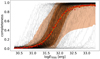 |
Fig. 13. Flare recovery rate calculated for each light curve. The orange line shows the average curve for all stars and the red points show the completeness curve calculated for a concatenated light curve. The shaded regions show the 1σ and 2σ confidence intervals. |
The reliability of the ED estimation method was also tested in a similar manner, by injecting artificial flares into the light curves. Owing to the high photometric noise, the measured differences in ED can exceed the nominal uncertainties. For flares above ETESS = 1032 erg, the measured EDs were erroneous by a factor of 10 in ∼5% of the injected flares. However, the differences are not expected to be this severe for most of the detected events, since we used all the light curves, even the noisiest, for the injection tests.
3.4. Hα emission
To look for emission features, we checked the Rizzo Spectral Library. Of those in our sample, 95 stars had available optical spectra, published by Cruz et al. (2003, 2007), and Reid et al. (2008). The average wavelength range of these spectra is from 5600 Å to 10000 Å with average  resolution between 2000 and 5000. Most stars showed prominent emission in Hα. We calculated the Hα equivalent width (EW) by integrating the flux between 6553 and 6573 Å, after normalising by a linear fit to the local continuum. The uncertainty of the EW was estimated by resampling from the flux errors. We note that the flux error bars were generally larger in the vicinity of Hα if the emission was stronger, leading to high (and possibly overestimated) uncertainties even for high EW values. The measured EWs are listed in Table 2.
3.5. Age determination
To see how the activity signatures evolve, it would be interesting to have an age estimation for as many stars from the sample as possible. While TRAPPIST–1 itself is fairly old (7.6 ± 2.2 Gyr, Burgasser & Mamajek 2017), the sample discussed in this work should include objects with different ages, since these low-mass objects move on the Hertzsprung–Russell diagram slowly during their evolution, while the selection criteria were related to color and luminosity alone. Unfortunately, all the other parameters of these stars evolve slowly with age, making the inference troublesome. In this section we explore the available methods to estimate stellar ages in this low-mass regime.
While the ages of individual objects are hard to estimate, it is not the case for clusters and moving groups. With available astrometric information the probability that these stars are members of known moving groups can be estimated. To this end, we utilized BANYAN Σ (Gagné et al. 2018). It can predict membership probabilities for 27 young associations within 150 pc, using position and velocity information. No stars in the sample had measured radial velocity in Gaia DR2, but 72 of these stars had literature measurements in the Simbad database. For these stars, we used all six-dimensional position and velocity information, while we omitted the radial velocity for the remaining objects. Fourteen stars had membership probability over 95%. Gaia DR2 65638443294980224, 3200303384927512960, 4900323420040865792, and 89186168428165632 had high membership probability and confirmation from the literature (Goldman et al. 2013; Baron et al. 2019; Gagné et al. 2015 and Bardalez Gagliuffi et al. 2019, respectively). Burgasser et al. (2015) find that Gaia DR2 6224387727748521344 does not show signs of young age, so it was rejected as an AB Doradus member. Although the remaining stars have no confirmation of young age from the literature nor measured radial velocity, they were kept as candidate moving group members.
For those 72 stars that had radial velocity measurements, the full six-dimensional position and velocity information are available. This lends itself to kinematic age estimation, which is a method that uses the motion within the galactic disk as a proxy for age. Young objects tend to have simple orbits with smaller peculiar velocities, while older stars are scattered to more eccentric and inclined orbits. We used the method of Almeida-Fernandes & Rocha-Pinto (2018) to calculate the age probability density function (PDF) from the UVW galactic velocity components. The method is calibrated using isochronal ages of ∼14 000 stars from the Geneva–Copenhagen Survey. While most of the other methods (such as isochrone fitting) are not applicable to low-mass stars, there is no mass dependence in the kinematic method. As a downside, the precision is low; the 1σ error bars are typically 2–3 Gyr.
First we converted the Gaia DR2 position, proper motion, parallax, and literature radial velocity data to galactic velocity components. The measurement uncertainties were propagated into the UVW components by resampling the input values. We then used the “UVW method” described in Sect. 3.1 of Almeida-Fernandes & Rocha-Pinto (2018), by calculating the components of the velocity ellipsoid and building the age PDF as a product of three Gaussians. To extract a point estimate from the PDF, we calculated the most likely age (tML) as the mode of the distribution and the expected age (tE) as
 (5)
(5)
where p(t|U, V, W) is the age PDF calculated numerically between 0 and 13.8 Gyr. Following the suggestions of Almeida-Fernandes & Rocha-Pinto (2018), we used the following kinematic age as the estimated value:
 (6)
(6)
with the uncertainty of
![Mathematical equation: $$ \begin{aligned} \delta _t = \frac{1}{4} \left[ (t_{84} - t_{16}) + \frac{t_{97.5} - t_{2.5}}{2} \right] , \end{aligned} $$](/articles/aa/full_html/2021/06/aa40098-20/aa40098-20-eq22.gif) (7)
(7)
where the subscripts of t denote percentiles. In the case of Gaussian distribution δt corresponds to 1σ. To take the measurement uncertainty of the UVW components into account, 100 realizations of the PDF were calculated using resampled UVW values and the point estimates were calculated from the median PDF. We also chose to add the scatter in the 100 individual tkin values in quadrature to δt, which generally increased δt by ∼0.1 Gyr. To illustrate the method, an example PDF can be seen in Fig. 14.
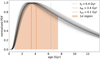 |
Fig. 14. Kinematic age PDF of Gaia DR2 3421840993510952192, where (U, V, W) = (33.0 ± 4.0, −20.5 ± 0.2, −22.2 ± 0.5) km s−1. The thin black lines show 100 realizations of the PDF taking into account measurement errors. |
Another technique to determine ages of UCDs is to look for wide binary pairs, where the age of the other component can be measured (assuming coevality). For all stars in the sample, we queried Gaia DR2 looking for stars with similar astrometric parameters. For this we utilized the same criteria as proposed by Smart et al. (2019), except that our search was limited to a projected separation of 0.2 pc. This resulted in 19 comoving pair candidates, with 0.05 pc maximum separation, summarised in Table C.1. Radial velocity measurement was available for nine stars, making kinematic age estimation possible.
Out of these 19 stars, Gaia DR2 1412377317863375488 has measured rotational period, but no kinematic age estimate. Its comoving pair is HD 234344, a bright K3 dwarf with measured radial velocity from Gaia DR2. The kinematic method gives 3.7 ± 3.3 Gyr, while isochrone fitting combined with gyrochronology with STARDATE (Angus et al. 2019) gives  Gyr (using the peak of the age posterior). We used 3.1853d ± 0.004d rotational period measured from three sectors of TESS FFI data.
As an independent means of age estimation, we inspected all the available optical spectra from the Rizzo Spectral Library looking for lithium absorption around 6708 Å and found none. The lithium depletion occurs around 100–200 Myr for stars in the mass range of 0.06–0.08 M⊙ (Burke et al. 2004), thus giving a lower limit for the age of these 95 stars. This rules out Gaia DR2 2755265775727402112, as BANYAN Σ gives 97% Columba membership probability, while the age of the association is only 42 Myr (Bell et al. 2015); thus the star should still show lithium absorption.
To summarise, we have age estimates from the following sources (prioritizing them in the following order, removing intersections): 12 from moving group membership, 5 from comoving pairs and 71 from kinematics. These are tabulated in Table 2 and their distribution is plotted in Fig. 15. The number of stars in our sample with different estimated parameters are shown in Fig. 16.
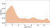 |
Fig. 15. Distribution of the ages of the stars in the sample. The kernel density estimation is calculated with Gaussian kernel with 0.6 Gyr bandwidth. The ticks below the curve show the individual data points. |
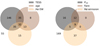 |
Fig. 16. Venn diagrams with the main properties of our sample. Left: number of stars with available TESS light curve, age estimate and calculated Hα EW from the whole sample of 339 stars. Right: number of stars with detected period, flaring, and Hα emission (where the EW is at least 1σ above zero), only for the 248 stars with available TESS observation. |
4. Results and discussion
4.1. Notes on individual stars
The most flaring stars of the sample are Gaia DR2 1295931997030930432 (5 flares), 3200303384927512960 (ten flares), and 4989399774745144448 (five flares). Figure 17 shows the available TESS light curves. Taking into account their different apparent magnitudes, these stars show a flaring rate comparable to TRAPPIST–1, as the downgraded K2 light curve from Sect. 3.3.1 yielded eight flare events in 70d of observation. While there is no trace in the literature of Gaia DR2 1295931997030930432, we know a bit more about the other two stars. Gaia DR2 3200303384927512960 (= 2MASS J04402325-0530082) appears in the sample of surveying nearby M dwarfs searching for brown dwarfs in Nguyen-Thanh et al. (2020), where a spectral energy distribution (SED) fit is presented with Teff = 2600 K and log g = 4.5. Gaia DR2 4989399774745144448 (= 2MASS J01025100-3737438) is listed as a flaring star by Mondrik et al. (2019) using observations from the MEarth photometric survey. Finally, we note that the well-known and observed flare star Gaia DR2 4339417394313320192 = vB8 (2MASS J16553529-0823401), which has a measured magnetic field (2.8 ± 0.4 kG, Shulyak et al. 2019), is also included in our sample, but has not been observed by TESS yet.
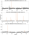 |
Fig. 17. Three most flaring targets from the sample, with |


4.2. Periods
Photometric observations of TRAPPIST–1 yielded different values for its rotational period: 0.819d from Spitzer infrared data (Roettenbacher & Kane 2017), 1.60d from TRAPPIST-South (Gillon et al. 2016), and 3.30d from K2 (Luger et al. 2017; Vida et al. 2017). The reason for the discrepancy could be the changing pattern of spots on the surface that could imitate, for example, half or one-fourth of the real period. This effect of a quickly evolving spot pattern was not observed in our sample, mainly as a consequence of the relatively short observing time. Out of the 42 stars with periodic signal, Gaia DR2 1656001233124961152 was observed for the longest time (11 sectors). To find potential evidence of a changing spot pattern, we compared the Lomb-Scargle periodograms of each sector and employed short-term Fourier transform (see, e.g., Kolláth & Oláh 2009). While the main period was only detected in 7 out of the 11 sectors, it is unclear whether the nondetections stem from some change in spot configuration or just data systematics and noise. Half of this period was not detected in any of the sectors.
The histogram of the detected periods of TRAPPIST–1 analogs is plotted in Fig. 8. The distribution seems to be unimodal and follow a log-normal distribution. We performed a Shapiro–Wilk test (Shapiro & Wilk 1965) on the logarithm of the periods, and it could not reject the null hypothesis of normal distribution (p = 0.37). As a test for unimodality, we fitted the log Prot dataset with a mixture of N Gaussians. The N = 1 model was clearly preferred by the Bayesian information criterion (with μ = 0.6d mean and σ = 0.6d scatter). To put this into context, we compare this with other distributions from the literature. We try to separate each distribution using Gaussian mixture models with the number of components determined from the Bayesian information criterion. We note that we use the logarithm of the periods, but transform the values back to make comparison easier.
The period distribution of early-to-mid M dwarfs in the Kepler field was drawn first by McQuillan et al. (2013) based on ten months of data. While they found a distinct group of shorter period stars making up ∼8% of the full sample, the most striking feature is the emergence of bimodality for longer periods, possibly arising from two distinct waves of star formation. The best Gaussian mixture fit is achieved with the following three components: (μ1, σ1) = (3d, 3d) for the fast rotators, and (μ2, σ2) = (18d, 4d), and (μ3, σ3) = (34d, 7d) for the longer periods. Later, Rappaport et al. (2014), using all 16 quarters of Kepler data, detailed the period distribution of 297 M dwarfs in the short period range. A two-component fit to their data yields (μ1, σ1) = (0.4d, 0.2d), (μ2, σ2) = (1.2d, 0.4d). Using ground-based photometry from the MEarth Project, Newton et al. (2016, 2018) compile the rotational period of ∼600 mid-to-late M dwarfs, also finding bimodality in the distribution. Fitting a Gaussian mixture model to the logarithm of Grade A and B rotational periods from Newton et al. (2016, 2018) gives the following parameters: (μ1, σ1) = (0.6d, 0.5d) for fast rotators, (μ2, σ2) = (93d, 25d) for slow rotators, and a wide (possibly background) component in between of (μ3, σ3) = (6d, 9d).
These support that the cutoff in Fig. 8 is not entirely due to the 5d upper limit in our period detection method, but there are a dearth of objects with periods above a few days. Also the distribution seems to be consistent with the MEarth dataset, even with the truncation. It is likely that many stars from our sample belong to the slow rotating group (Prot ∼ 100d), making one or two sectors of TESS data insufficient to reliably measure their periods.
Figure 18 shows a very weak correlation between log Prot and age, if any (0.43 Pearson correlation coefficient, where p = 0.09). There are several ways in which Prot can evolve (see Bouvier et al. 2014 for an overview), one of which is the initial spin up due to contraction. However, the stars in our sample are likely older than the typical spin-up timescale, as illustrated in Fig. 20. After reaching the main sequence, UCDs evolve slowly, losing angular momentum with stellar wind. While this mechanism is effective for solar-type stars, UCDs spin down slowly, retaining their fast rotation for billions of years (see, e.g., Reiners & Mohanty 2012; Newton et al. 2016). Irwin et al. (2011) studied a sample of 41 fully convective field M dwarfs with Prot measured from MEarth data. In their Fig. 13, they show age versus Prot for their sample and also for several open clusters. Viewing only stars older than ∼10 Myr and with Prot < 10d gives a similarly large scatter as in Fig. 18 in this paper.
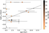 |
Fig. 18. Age and rotational periods for the sample. The dashed line shows a linear fit and the small black points show stars without Hα EW measurement. |
According to Fig. 19, the Hα emission does not seem to correlate with age or Prot. A possible explanation could be the saturated activity in these late-type stars. Roettenbacher & Kane (2017) show that the Rossby number R0 = Prot/τc is below 0.1 for TRAPPIST–1, and in fact for all stars with measured Prot in our sample, taking τc = 70d for the convective turnover time (following Reiners & Basri 2010). This means that the rotation rate no longer influences the activity of the 42 fast rotators found in this work. It can be seen in Fig. 16 that one-fourth of the stars with detected Hα emission are fast rotators.
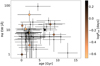 |
Fig. 19. Age and Hα emission. There appears to be no clear trend with the rotational period. |
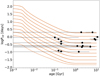 |
Fig. 20. Rotational period vs. age for the TRAPPIST–1 analogs, compared with M = 0.09 M⊙ evolutionary tracks from Baraffe et al. (2015), assuming angular momentum conservation with different initial Prot values. The dashed line shows the breakup period Pcrit[days] = 0.116(R/R⊙)3/2(M/M⊙)−1/2 from Herbst et al. (2001). |
4.3. Flare frequency distribution
With the estimated flare energies from Sect. 3.3, the cumulative number of flares above given energies, the FFD, is shown in Fig. 21. This includes flares from 21 stars, all of which have measured rotational periods (see Fig. 16). We note that normally the FFD is plotted only for a single star, but we used the whole sample because most flaring stars showed only one event. This way, the composite FFD can be treated as an “average” FFD of the whole sample, including stars with different parameters, most notably different ages. However, according to Figs. 18 and 19 the ages of the stars do not really affect their activity levels, that is, no clear trend is found between the age and the rotational periods and/or Hα emission. The original FFD was corrected by dividing with the averaged completeness curve shown in Fig. 13. The corrected FFD was fitted with a linear function on log–log scale, yielding
![Mathematical equation: $$ \begin{aligned} \log (\nu [\mathrm{day} ^{-1}]) = (-1.11 \pm 0.02) \log (E_{\mathrm{TESS} } [\mathrm{erg} ]) + (33.4 \pm 0.8), \end{aligned} $$](/articles/aa/full_html/2021/06/aa40098-20/aa40098-20-eq27.gif) (8)
(8)
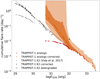 |
Fig. 21. Composite FFD for the whole sample. Red points are the original values, orange points are corrected for flare recovery rate (orange line in Fig. 13), and shaded regions are the 1 and 2σ confidence intervals. The FFD of TRAPPIST–1 with K2 short cadence data from Vida et al. (2017) is also plotted for reference, converted to the TESS bandpass, and also its correction for completeness. Grey circles shows the flares recovered from the K2 light curve of TRAPPIST–1 downgraded to imitate a hypothetical TESS observation (with added noise, and re-sampled to 30-min cadence). Dashed lines show linear fits. |
where ν is the cumulative flare rate. This results in α = 2.11 ± 0.02 power-law index, where
 (9)
(9)
As the uncertainty from the completeness correction was taken into account in the fit, the lower energy part had only negligible contribution. Fitting only above the break point at log ETESS = 32 gives α = 2.11 ± 0.05.
Vida et al. (2017) created the FFD of TRAPPIST–1 using short cadence Kepler K2 data. To compare the flare energies between Kepler and TESS, we calculated an approximate conversion factor by assuming (9000 ± 500) K blackbody spectrum for the emitting region (Kretzschmar 2011). We then convolved the spectral response functions of the instruments with the blackbody spectrum, and integrated over wavelength. Thus, the flare energies from Kepler can be converted to flare energies in the TESS bandpass as follows:
 (10)
(10)
This results in a 0.14 shift on logarithmic energy scale. Similarly, an approximate conversion factor to bolometric flare energy was calculated using a (9000 ± 500) K blackbody as follows:
 (11)
(11)
We note that while the Kepler–TESS conversion was relatively insensitive to the assumed blackbody temperature, this is not the case for the bolometric conversion. While T = 9000 K is generally used in the literature for the effective flare temperature (see, e.g., Osten & Wolk 2015), Howard et al. (2020) demonstrate that superflares can emit at significantly higher temperatures. So the bolometric flare energies should be treated with caution because they are likely lower limits. Before applying Eq. (10), the K2 flare energies were recalculated using LKepler = 5.6 × 1028 erg s−1 from Sect. 3.3, since Vida et al. (2017) use a different luminosity. Figure 21 also shows the K2 FFD and its downgraded version from Sect. 3.3.1. The measurements presented in this work are complementary to TRAPPIST–1, as they probe a higher energy range not observed before. The K2 FFD was also fitted with a line on log–log scale, taking into account the completeness correction from Sect. 3.3.2, and omitting the highest energy point, which seems to deviate from the trend, resulting in
![Mathematical equation: $$ \begin{aligned} \log (\nu [\mathrm{day} ^{-1}]) = (-1.03 \pm 0.02) \log (E_{\mathrm{TESS} } [\mathrm{erg} ]) + (30.7 \pm 0.6). \end{aligned} $$](/articles/aa/full_html/2021/06/aa40098-20/aa40098-20-eq31.gif) (12)
(12)
This yields α = 2.03 ± 0.02 for TRAPPIST–1, a value consistent with that found for our sample, suggesting that the FFD can be described by a single power law. Not using the correction for recovery rate would give α = 1.59 ± 0.02, which is a significantly shallower slope.
Hawley et al. (2014) analyse the flare rate of early-to-mid M dwarfs with Kepler short cadence data and find the steepest power-law index α = 2.32 on the latest M-dwarf binary in their sample, GJ 1245 AB (M5+M5). Once the light curve of the binary was separated by Lurie et al. (2015), the two independent power-law indices changed to α = 1.99 ± 0.02 and α = 2.03 ± 0.02. Paudel et al. (2018) use K2 light curves to study flares on ten UCDs (including TRAPPIST–1) and find α ranging from 1.34 to 2.04, with 1.66 mean. Gizis et al. (2017) use K2 data to study three young UCDs, and found α = 1.8. For the mid-to-late M dwarf sample of Medina et al. (2020), the power-law index is α = 1.98 ± 0.02. Yang & Liu (2019) compiled a catalog of flares using all available long cadence Kepler light curves from DR25. These authors find an average α ≈ 2 power-law index for all spectral types excluding A stars as well as a ∼10% incidence rate of flare stars among M dwarfs that is consistent with our result (∼8%). So it appears that the slope found for the TRAPPIST–1 analogs in this work (α = 2.11) is typical for late M dwarfs, and consistent with TRAPPIST–1 itself (α = 2.03). It also confirms that the same power-law index is further applicable for one or two orders of magnitude larger flares. According to Aschwanden et al. (2016), magnetic and thermal energies dominate around α ≈ 2.0 as opposed to nonthermal energy around α ≈ 1.4.
4.4. Habitability
Out of a sample of 57 exoplanets studied by Jagadeesh et al. (2018), TRAPPIST–1f is the closest to Earth in terms of the Earth Similarity Index, Active Tardigrade Index, and Cryptobiotic Tardigrade Index, meaning that life, as we know it, may survive on its surface (especially extremophile organisms such as tardigrades). And while Kepler searched for exoplanets around solar-like stars, the number of detections around M dwarfs is expected to grow with TESS. So the question of habitability around UCDs, especially TRAPPIST–1, is timely.
Late-type dwarfs are important for exoplanet habitability studies since they spend billions of years on the main sequence, giving life enough time to emerge on the surface of planets orbiting them. However, the magnetic activity of these stars can endanger the habitability of the orbiting planets. One of the hazards is the erosion of the planetary atmosphere through intense electromagnetic and particle radiation. To preserve their atmospheres, the planets need a strong magnetic field, even 10–1000 times stronger than Earth’s magnetosphere (Vidotto et al. 2013). We know from the Sun that a large portion of flares are accompanied by CMEs, which are especially harmful if they reach the planetary atmosphere. Apart from the magnetosphere of the planets, Mullan et al. (2018) argue that the host star itself can trap the CMEs if it has sufficient magnetic field. They calculate a global 1.4–1.75 kG dipole field for TRAPPIST–1, which is strong enough to suppress even 1034 − 1035 erg events, assuming that flares are accompanied by CMEs with comparable energy. Furthermore, successful CMEs seem to be very rare in late-type dwarfs empirically, 90–98% of the eruptions do not reach the escape velocity, suggesting that electromagnetic radiation would be a larger factor for atmosphere erosion than particles (Vida et al. 2016, 2019a). This suggests that the planets of TRAPPIST–1 are safe CME-wise assuming the FFD from Fig. 21. And even if energetic flares/CMEs were to erode the atmosphere of young planets and deplete their water reservoir in the early stages of their evolution, the replenishment of the ocean is possible through asteroid bombardment events (Dencs & Regály 2019). In this scenario, late M dwarfs are not likely to erode their secondary atmospheres after their primordial H/He envelope is gone (Atri & Mogan 2021). Dong et al. (2018) reach a similar conclusion for TRAPPIST–1, showing that the outer planets can retain their atmospheres for billions of years.
Once an atmosphere or even an ocean is present, abiogenesis is possible. The other hazardous effect of magnetic activity is the increased UV radiation during stellar flares that could harm simple or more evolved organisms; we note however that the UV radiation of flares might be the source that powers prebiotic photochemistry (see, e.g., Ranjan et al. 2017). Estrela et al. (2020) studied the impact of superflares on two different bacteria (E. coli and D. radiodurans) on the TRAPPIST–1 planets. They find that an ozone layer or a few meters deep ocean is sufficient for the bacteria to survive the largest flares observed by Kepler K2. Abrevaya et al. (2020) show that ozone is not the only option for a protective atmosphere, and a combination of CO2 and N2 could also suffice. Also, Chen et al. (2021) show that larger flares can permanently change the composition of exoplanet atmospheres, driving them toward a different equilibrium state.
The FFD presented in this work includes flares with higher energies than ever observed on TRAPPIST–1 before, and it seems that the FFD can still be described by a single power law with α ≈ 2. Figure 22 shows the schematic FFD along with regions where ozone depletion and abiogenesis can be expected. Tilley et al. (2019) estimate that the ozone layer of unmagnetized planets can be fully destroyed if the rate of Ebol > 1034 erg superflares reaches 0.1 day−1. According to Rimmer et al. (2018), the lower limit on the FFD where abiogenesis is possible is also a power law, with −1 exponent. Their original relation used U-band energy, but we adopt the formula of Glazier et al. (2020) with Ebol (using blackbody conversion factors from Osten & Wolk 2015), thus giving
 (13)
(13)
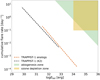 |
Fig. 22. Flare frequency distribution showing the region where abiogenesis is possible (Rimmer et al. 2018) and where ozone depletion can occur (Tilley et al. 2019), following Günther et al. (2020). The dashed lines indicate the linear fits from Fig. 21; Ebol is used instead of ETESS. |
And since α ≈ 2 corresponds to 1 − α ≈ −1 exponent, the border of the abiogenesis zone is approximately parallel to the FFD of TRAPPIST–1, hinting that they do not intersect, not even at higher energies. This strengthens the findings of Glazier et al. (2020), who find that the current flare rate of TRAPPIST–1 is unlikely to cause ozone depletion or initiate abiogenesis.
5. Summary and conclusions
Using simple photometric criteria, we compiled a list of TRAPPIST–1 analogs, and analysed the 30 min TESS light curves of 248 of these stars. To characterize their magnetic activity, we looked for flares and rotational periods. We can summarise our findings as follows:
-
We found a total of 94 flare events on 21 stars. Of the targets, a periodic light curve modulation was found in 42 (likely due to rotation) in the range of 0.1–5d ; we only searched for periods up to 5d. All the 21 stars with flares show rotational modulation as well.
-
We estimated the approximate age of 88 stars from the sample with various methods, but did not find a convincing correlation between age, rotation rate, and Hα emission.
-
The power-law slope of the composite FFD was found to be similar to the value for TRAPPIST–1, hinting that it is not an especially active/inactive star for its spectral type. Combining the light curves of objects in the sample enabled us to find stronger flares than ever observed on TRAPPIST–1 before, suggesting that they occur, even if rarely. We found that flares with ETESS > 1033 erg (Ebol ≳ 1034 erg) can be expected every few decades.
-
Is seems that the flaring rate of TRAPPIST–1 is not sufficient to fully destroy the possible ozone layer of its planets nor to initiate abiogenesis via UV radiation. Glazier et al. (2020) reach a similar conclusion, using an upper limit for the super-flare rate from Evryscope observations.
As TESS continues its mission, it is possible to keep observing ultracool dwarfs, to have a larger temporal baseline for rotational periods and possible changes in spot configuration. With the inclusion of the ecliptic, the missing TRAPPIST–1 analogs could also be observed. Future studies of stellar flares could also benefit from the higher cadence of full-frame images starting from Sector 27, making it possible to find shorter flares.
Acknowledgments
The authors would like to thank the anonymous referee for improving the quality of the paper with helpful comments and suggestions. BS was supported by the ÚNKP-19-3 New National Excellence Program of the Ministry for Innovation and Technology. KV was supported by the Bolyai János Research Scholarship of the Hungarian Academy of Sciences. This project has been supported by the Lendület Program of the Hungarian Academy of Sciences, project No. LP2018-7/2019, the NKFI KH-130526 and NKFI K-131508 grants, the Hungarian OTKA Grant No. 119993 and by the NKFI grant 2019-2.1.11-TÉT-2019-00056. On behalf of “Analysis of space-borne photometric data” project we thank for the usage of MTA Cloud (https://cloud.mta.hu) that helped us achieving the results published in this paper. Authors acknowledge the financial support of the Austrian-Hungarian Action Foundation (95 öu3, 98öu5, 101öu13). This paper includes data collected by the TESS mission. Funding for the TESS mission is provided by the NASA Explorer Program. This research has benefitted from the Ultracool RIZzo Spectral Library (http://dx.doi.org/10.5281/zenodo.11313), maintained by Jonathan Gagné and Kelle Cruz.
References
- Abrevaya, X. C., Leitzinger, M., Oppezzo, O. J., et al. 2020, MNRAS, 494, L69 [Google Scholar]
- Almeida-Fernandes, F., & Rocha-Pinto, H. J. 2018, MNRAS, 476, 184 [Google Scholar]
- Alvarado-Gómez, J. D., Drake, J. J., Cohen, O., Moschou, S. P., & Garraffo, C. 2018, ApJ, 862, 93 [NASA ADS] [CrossRef] [Google Scholar]
- Anglada-Escudé, G., Amado, P. J., Barnes, J., et al. 2016, Nature, 536, 437 [NASA ADS] [CrossRef] [PubMed] [Google Scholar]
- Angus, R., Morton, T. D., Foreman-Mackey, D., et al. 2019, AJ, 158, 173 [Google Scholar]
- Aschwanden, M. J., Holman, G., O’Flannagain, A., et al. 2016, ApJ, 832, 27 [NASA ADS] [CrossRef] [Google Scholar]
- Atri, D., & Mogan, S. R. C. 2021, MNRAS, 500, L1 [Google Scholar]
- Baraffe, I., Homeier, D., Allard, F., & Chabrier, G. 2015, A&A, 577, A42 [NASA ADS] [CrossRef] [EDP Sciences] [Google Scholar]
- Bardalez Gagliuffi, D. C., Burgasser, A. J., Schmidt, S. J., et al. 2019, ApJ, 883, 205 [Google Scholar]
- Baron, F., Lafrenière, D., Artigau, É., et al. 2019, AJ, 158, 187 [Google Scholar]
- Bell, C. P. M., Mamajek, E. E., & Naylor, T. 2015, MNRAS, 454, 593 [NASA ADS] [CrossRef] [Google Scholar]
- Bouvier, J., Matt, S. P., Mohanty, S., et al. 2014, in Protostars and Planets VI, eds. H. Beuther, R. S. Klessen, C. P. Dullemond, & T. Henning, 433 [Google Scholar]
- Burgasser, A. J., & Mamajek, E. E. 2017, ApJ, 845, 110 [NASA ADS] [CrossRef] [Google Scholar]
- Burgasser, A. J., Logsdon, S. E., Gagné, J., et al. 2015, ApJS, 220, 18 [NASA ADS] [CrossRef] [Google Scholar]
- Burke, C. J., Pinsonneault, M. H., & Sills, A. 2004, ApJ, 604, 272 [NASA ADS] [CrossRef] [Google Scholar]
- Chen, H., Zhan, Z., Youngblood, A., et al. 2021, Nat. Astron., 5, 298 [Google Scholar]
- Cleveland, W. S. 1979, J. Am. Stat. Assoc., 74, 829 [Google Scholar]
- Cruz, K. L., Reid, I. N., Liebert, J., Kirkpatrick, J. D., & Lowrance, P. J. 2003, AJ, 126, 2421 [NASA ADS] [CrossRef] [Google Scholar]
- Cruz, K. L., Reid, I. N., Kirkpatrick, J. D., et al. 2007, AJ, 133, 439 [Google Scholar]
- Davenport, J. R. A. 2016, ApJ, 829, 23 [Google Scholar]
- Davenport, J. R. A., Hawley, S. L., Hebb, L., et al. 2014, ApJ, 797, 122 [Google Scholar]
- Dencs, Z., & Regály, Z. 2019, MNRAS, 487, 2191 [Google Scholar]
- Dong, C., Jin, M., Lingam, M., et al. 2018, Proc. Nat. Acad. Sci., 115, 260 [Google Scholar]
- Estrela, R., Palit, S., & Valio, A. 2020, Astrobiology, 20, 1465 [Google Scholar]
- Fonnesbeck, C., Patil, A., Huard, D., & Salvatier, J. 2015, PyMC: Bayesian Stochastic Modelling in Python [Google Scholar]
- Gagné, J., Lafrenière, D., Doyon, R., Malo, L., & Artigau, É. 2015, ApJ, 798, 73 [NASA ADS] [CrossRef] [Google Scholar]
- Gagné, J., Mamajek, E. E., Malo, L., et al. 2018, ApJ, 856, 23 [NASA ADS] [CrossRef] [Google Scholar]
- Gaia Collaboration (Brown, A. G. A., et al.) 2018, A&A, 616, A1 [NASA ADS] [CrossRef] [EDP Sciences] [Google Scholar]
- Gaia Collaboration (Smart, R. L., et al.) 2021, A&A, 649, A6 [EDP Sciences] [Google Scholar]
- Gershberg, R. E. 1972, Ap&SS, 19, 75 [Google Scholar]
- Gillon, M., Jehin, E., Lederer, S. M., et al. 2016, Nature, 533, 221 [Google Scholar]
- Gillon, M., Triaud, A. H. M. J., Demory, B.-O., et al. 2017, Nature, 542, 456 [Google Scholar]
- Gizis, J. E., Paudel, R. R., Mullan, D., et al. 2017, ApJ, 845, 33 [NASA ADS] [CrossRef] [Google Scholar]
- Glazier, A. L., Howard, W. S., Corbett, H., et al. 2020, ApJ, 900, 27 [Google Scholar]
- Goldman, B., Röser, S., Schilbach, E., et al. 2013, A&A, 559, A43 [NASA ADS] [CrossRef] [EDP Sciences] [Google Scholar]
- Gonzales, E. C., Faherty, J. K., Gagné, J., et al. 2019, ApJ, 886, 131 [Google Scholar]
- Günther, M. N., Zhan, Z., Seager, S., et al. 2020, AJ, 159, 60 [CrossRef] [Google Scholar]
- Hawley, S. L., Davenport, J. R. A., Kowalski, A. F., et al. 2014, ApJ, 797, 121 [NASA ADS] [CrossRef] [Google Scholar]
- Herbst, W., Bailer-Jones, C. A. L., & Mundt, R. 2001, ApJ, 554, L197 [NASA ADS] [CrossRef] [Google Scholar]
- Howard, W. S., Corbett, H., Law, N. M., et al. 2020, ApJ, 902, 115 [Google Scholar]
- Irwin, J., Berta, Z. K., Burke, C. J., et al. 2011, ApJ, 727, 56 [Google Scholar]
- Jagadeesh, M. K., Roszkowska, M., & Kaczmarek, Ł. 2018, Life Sci. Space Res., 19, 13 [NASA ADS] [CrossRef] [Google Scholar]
- Jordi, C., Gebran, M., Carrasco, J. M., et al. 2010, A&A, 523, A48 [NASA ADS] [CrossRef] [EDP Sciences] [Google Scholar]
- Kolláth, Z., & Oláh, K. 2009, A&A, 501, 695 [NASA ADS] [CrossRef] [EDP Sciences] [Google Scholar]
- Kretzschmar, M. 2011, A&A, 530, A84 [NASA ADS] [CrossRef] [EDP Sciences] [Google Scholar]
- Lomb, N. R. 1976, Ap&SS, 39, 447 [Google Scholar]
- Luger, R., Sestovic, M., Kruse, E., et al. 2017, Nat. Astron., 1, 0129 [Google Scholar]
- Lurie, J. C., Davenport, J. R. A., Hawley, S. L., et al. 2015, ApJ, 800, 95 [NASA ADS] [CrossRef] [Google Scholar]
- McQuillan, A., Aigrain, S., & Mazeh, T. 2013, MNRAS, 432, 1203 [Google Scholar]
- Medina, A. A., Winters, J. G., Irwin, J. M., & Charbonneau, D. 2020, ApJ, 905, 107 [Google Scholar]
- Mondrik, N., Newton, E., Charbonneau, D., & Irwin, J. 2019, ApJ, 870, 10 [NASA ADS] [CrossRef] [Google Scholar]
- Mullan, D. J., MacDonald, J., Dieterich, S., & Fausey, H. 2018, ApJ, 869, 149 [NASA ADS] [CrossRef] [Google Scholar]
- Namekata, K., Sakaue, T., Watanabe, K., et al. 2017, ApJ, 851, 91 [Google Scholar]
- Newton, E. R., Irwin, J., Charbonneau, D., et al. 2016, ApJ, 821, 93 [NASA ADS] [CrossRef] [Google Scholar]
- Newton, E. R., Mondrik, N., Irwin, J., Winters, J. G., & Charbonneau, D. 2018, AJ, 156, 217 [NASA ADS] [CrossRef] [Google Scholar]
- Nguyen-Thanh, D., Phan-Bao, N., Murphy, S. J., & Bessell, M. S. 2020, A&A, 634, A128 [EDP Sciences] [Google Scholar]
- Osten, R. A., & Wolk, S. J. 2015, ApJ, 809, 79 [NASA ADS] [CrossRef] [Google Scholar]
- Pál, A. 2012, MNRAS, 421, 1825 [NASA ADS] [CrossRef] [Google Scholar]
- Paudel, R. R., Gizis, J. E., Mullan, D. J., et al. 2018, ApJ, 858, 55 [Google Scholar]
- Petralia, A., & Micela, G. 2020, Exp. Astron., 49, 97 [Google Scholar]
- Raetz, S., Stelzer, B., Damasso, M., & Scholz, A. 2020, A&A, 637, A22 [NASA ADS] [CrossRef] [EDP Sciences] [Google Scholar]
- Ranjan, S., Wordsworth, R., & Sasselov, D. D. 2017, ApJ, 843, 110 [Google Scholar]
- Rappaport, S., Swift, J., Levine, A., et al. 2014, ApJ, 788, 114 [Google Scholar]
- Reid, I. N., Cruz, K. L., Kirkpatrick, J. D., et al. 2008, AJ, 136, 1290 [NASA ADS] [CrossRef] [Google Scholar]
- Reiners, A., & Basri, G. 2010, ApJ, 710, 924 [NASA ADS] [CrossRef] [Google Scholar]
- Reiners, A., & Mohanty, S. 2012, ApJ, 746, 43 [NASA ADS] [CrossRef] [Google Scholar]
- Reylé, C. 2018, A&A, 619, L8 [NASA ADS] [CrossRef] [EDP Sciences] [Google Scholar]
- Ricker, G. R., Winn, J. N., Vanderspek, R., et al. 2015, J. Astron. Telescopes Instrum. Syst., 1 [Google Scholar]
- Rimmer, P. B., Xu, J., Thompson, S. J., et al. 2018, Sci. Adv., 4, eaar3302 [Google Scholar]
- Roettenbacher, R. M., & Kane, S. R. 2017, ApJ, 851, 77 [Google Scholar]
- Scargle, J. D. 1982, ApJ, 263, 835 [Google Scholar]
- Shapiro, S. S., & Wilk, M. B. 1965, Biometrika, 52, 591 [Google Scholar]
- Shulyak, D., Reiners, A., Nagel, E., et al. 2019, A&A, 626, A86 [NASA ADS] [CrossRef] [EDP Sciences] [Google Scholar]
- Smart, R. L., Marocco, F., Sarro, L. M., et al. 2019, MNRAS, 485, 4423 [Google Scholar]
- Stassun, K. G., Oelkers, R. J., Paegert, M., et al. 2019, AJ, 158, 138 [Google Scholar]
- Tenenbaum, P., & Jenkins, J. M. 2018, TESS Science Data Products Description Document, EXP-TESSARC-ICD-0014 Rev D (Baltimore, MD: STScI), https://archive.stsci.edu/missions/tess/doc/EXP-TESS-ARC-ICD-TM-0014.pdf [Google Scholar]
- Tilley, M. A., Segura, A., Meadows, V., Hawley, S., & Davenport, J. 2019, Astrobiology, 19, 64 [Google Scholar]
- Van Doorsselaere, T., Shariati, H., & Debosscher, J. 2017, ApJS, 232, 26 [NASA ADS] [CrossRef] [Google Scholar]
- Vida, K., Kriskovics, L., Oláh, K., et al. 2016, A&A, 590, A11 [NASA ADS] [CrossRef] [EDP Sciences] [Google Scholar]
- Vida, K., Kővári, Z. s., Pál, A., Oláh, K., & Kriskovics, L. 2017, ApJ, 841, 124 [NASA ADS] [CrossRef] [Google Scholar]
- Vida, K., Leitzinger, M., Kriskovics, L., et al. 2019a, A&A, 623, A49 [NASA ADS] [CrossRef] [EDP Sciences] [Google Scholar]
- Vida, K., Oláh, K., Kővári, Z. s., et al. 2019b, ApJ, 884, 160 [NASA ADS] [CrossRef] [Google Scholar]
- Vidotto, A. A., Jardine, M., Morin, J., et al. 2013, A&A, 557, A67 [NASA ADS] [CrossRef] [EDP Sciences] [Google Scholar]
- Yang, H., & Liu, J. 2019, ApJS, 241, 29 [CrossRef] [Google Scholar]
- Zechmeister, M., Dreizler, S., Ribas, I., et al. 2019, A&A, 627, A49 [NASA ADS] [EDP Sciences] [Google Scholar]
- Zhan, Z., Günther, M. N., Rappaport, S., et al. 2019, ApJ, 876, 127 [Google Scholar]
Appendix A: Measured rotational periods
We present the rotational periods in Table A.1. If the period was measurable in multiple sectors, the average period is given; the differences between the period values of the same star are consistent with the nominal error bars. In such cases the FAP value is calculated as the geometric mean of individual FAPs. The phase-folded light curves are plotted in Fig. A.1.
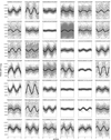 |
Fig. A.1. Light curves of stars with detected periodicity, folded with the average period from Table A.1. The black line denotes the smoothed light curve. |
Rotational periods from the Lomb–Scargle analysis.
Appendix B: Flare events
We present the parameters of all 94 individual flare events in Table B.1. In some cases the MCMC fit did not converge; for those events t1/2, fit, Afit and EDfit are omitted and tpeak, fit only indicates the time of the highest flux value.
Flare parameters.
Appendix C: Comoving pairs
We present the parameters of 19 comoving pair candidates in Table C.1.
Comoving pair candidates from Gaia DR2.
All Tables
SQL query used to select the sources from the Gaia DR2 catalog using the services provided by the Gaia TAP server.
All Figures
|
Fig. 1. Selection criteria on the Gaia color–magnitude diagram. The red point shows the position of TRAPPIST–1 and the orange points represent the final TRAPPIST–1 analog sample. The empty orange circles indicate stars that were not initially included as a result of the Gaia quality cuts, but were later added from existing UCD catalogs. |
| In the text | |
|
Fig. 2. Photometric properties of the sample. Left: brightness distribution of the final sample. Right: noise properties of the sample. The black curve shows the photometric scatter measured on the final processed light curves. The region between the 16th and 84th percentiles is shown in grey. The dashed line is the predicted noise value from TICgen. |
| In the text | |
|
Fig. 3. Position of the selected stars on the sky with equatorial coordinates, color coded with distance. The stars plotted with filled points have been observed by TESS up to Sector 26. The red circle represents TRAPPIST–1. The ecliptic is shown with a dashed line for reference. |
| In the text | |
|
Fig. 4. Field of view of a selected target (Gaia DR2 2883680659313632896) from Gaia, with 173 stars brighter than 20m. The red cross denotes the target, dashed circles show the aperture and annulus used for the TESS photometry, and solid circles show the stars selected for PCA. The grid in the background illustrates the pixel scale of TESS. |
| In the text | |
|
Fig. 5. Extracted light curves from the circular apertures of Fig. 4, with red dots indicating the celestial position of the sources. Some common trends can be identified, while the large flare seen on the target (red curve) does not seem to appear anywhere else. |
| In the text | |
|
Fig. 6. PCA reconstruction of the light curve from Fig. 5. The black points in the upper panel show the light curve created by QDLP_EXTRACT; the red curve shows the PCA reconstruction. The corrected light curve can be seen in the lower panel, showing a dominant flare and periodic variation. |
| In the text | |
|
Fig. 7. Period analysis for the corrected light curve from Fig. 6. Upper panel: light curve phase folded with the 1.93d period, which can be identified on the Lomb–Scargle periodogram below. |
| In the text | |
|
Fig. 8. Rotational period distribution of the sample with TESS. The one-dimensional kernel density estimation plotted with orange is calculated with a Gaussian kernel with bandwidth of 0.15. The black ticks show the individual period values. Only periods below 5d were kept owing to the 27d baseline of TESS sectors. |
| In the text | |
|
Fig. 9. Flare event fitted with the analytical template following the example of Fig. 6. The summed ED is 15.4 ± 2.9 min, while the fit gives 12.9 ± 4.4 min. |
| In the text | |
|
Fig. 10. Flare parameters from different methods. Left: comparison of the summed and fitted EDs. While they generally give the same result, they can differ by a factor of 2–3. Right: comparison of the observed flare amplitude (the highest flux value) and the fitted amplitude. Owing to the low time resolution, the observed peak is generally smaller. |
| In the text | |
|
Fig. 11. Correlations between the flare parameters. |
| In the text | |
|
Fig. 12. Kepler K2 light curve of TRAPPIST–1 from Vida et al. (2017) (black) rebinned to 30 min time resolution and with TESS-like scatter (red). The black and red ticks below the light curve indicate the position of flares found in the corresponding dataset. |
| In the text | |
|
Fig. 13. Flare recovery rate calculated for each light curve. The orange line shows the average curve for all stars and the red points show the completeness curve calculated for a concatenated light curve. The shaded regions show the 1σ and 2σ confidence intervals. |
| In the text | |
|
Fig. 14. Kinematic age PDF of Gaia DR2 3421840993510952192, where (U, V, W) = (33.0 ± 4.0, −20.5 ± 0.2, −22.2 ± 0.5) km s−1. The thin black lines show 100 realizations of the PDF taking into account measurement errors. |
| In the text | |
|
Fig. 15. Distribution of the ages of the stars in the sample. The kernel density estimation is calculated with Gaussian kernel with 0.6 Gyr bandwidth. The ticks below the curve show the individual data points. |
| In the text | |
|
Fig. 16. Venn diagrams with the main properties of our sample. Left: number of stars with available TESS light curve, age estimate and calculated Hα EW from the whole sample of 339 stars. Right: number of stars with detected period, flaring, and Hα emission (where the EW is at least 1σ above zero), only for the 248 stars with available TESS observation. |
| In the text | |
|
Fig. 17. Three most flaring targets from the sample, with |
| In the text | |
|
Fig. 18. Age and rotational periods for the sample. The dashed line shows a linear fit and the small black points show stars without Hα EW measurement. |
| In the text | |
|
Fig. 19. Age and Hα emission. There appears to be no clear trend with the rotational period. |
| In the text | |
|
Fig. 20. Rotational period vs. age for the TRAPPIST–1 analogs, compared with M = 0.09 M⊙ evolutionary tracks from Baraffe et al. (2015), assuming angular momentum conservation with different initial Prot values. The dashed line shows the breakup period Pcrit[days] = 0.116(R/R⊙)3/2(M/M⊙)−1/2 from Herbst et al. (2001). |
| In the text | |
|
Fig. 21. Composite FFD for the whole sample. Red points are the original values, orange points are corrected for flare recovery rate (orange line in Fig. 13), and shaded regions are the 1 and 2σ confidence intervals. The FFD of TRAPPIST–1 with K2 short cadence data from Vida et al. (2017) is also plotted for reference, converted to the TESS bandpass, and also its correction for completeness. Grey circles shows the flares recovered from the K2 light curve of TRAPPIST–1 downgraded to imitate a hypothetical TESS observation (with added noise, and re-sampled to 30-min cadence). Dashed lines show linear fits. |
| In the text | |
|
Fig. 22. Flare frequency distribution showing the region where abiogenesis is possible (Rimmer et al. 2018) and where ozone depletion can occur (Tilley et al. 2019), following Günther et al. (2020). The dashed lines indicate the linear fits from Fig. 21; Ebol is used instead of ETESS. |
| In the text | |
|
Fig. A.1. Light curves of stars with detected periodicity, folded with the average period from Table A.1. The black line denotes the smoothed light curve. |
| In the text | |
Current usage metrics show cumulative count of Article Views (full-text article views including HTML views, PDF and ePub downloads, according to the available data) and Abstracts Views on Vision4Press platform.
Data correspond to usage on the plateform after 2015. The current usage metrics is available 48-96 hours after online publication and is updated daily on week days.
Initial download of the metrics may take a while.