| Issue |
A&A
Volume 687, July 2024
|
|
|---|---|---|
| Article Number | A138 | |
| Number of page(s) | 10 | |
| Section | Stellar atmospheres | |
| DOI | https://doi.org/10.1051/0004-6361/202449541 | |
| Published online | 04 July 2024 | |
The corona of a fully convective star with a near-polar flare
1
Leibniz Institute for Astrophysics Potsdam (AIP),
An der Sternwarte 16,
14482
Potsdam,
Germany
2
ASTRON, Netherlands Institute for Radio Astronomy,
Oude Hoogeveensedijk 4,
Dwingeloo,
7991
PD,
The Netherlands
e-mail: This email address is being protected from spambots. You need JavaScript enabled to view it.
3
Institute for Physics and Astronomy, University of Potsdam,
Karl-Liebknecht-Strasse 24/25,
14476
Potsdam,
Germany
4
Institut für Astronomie & Astrophysik, Eberhard Karls Universität Tübingen,
Sand 1,
72076
Tübingen,
Germany
Received:
8
February
2024
Accepted:
6
May
2024
Abstract
Context. In 2020, the Transiting Exoplanet Survey Satellite (TESS) observed a rapidly rotating M7 dwarf, TIC 277539431, producing a flare at 81° latitude, the highest latitude flare located to date. This is in stark contrast to solar flares that occur much closer to the equator, typically below 30°. The mechanisms that allow flares at high latitudes to occur are poorly understood.
Aims. We studied five sectors of TESS monitoring, and obtained 36 ks of XMM-Newton observations to investigate the coronal and flaring activity of TIC 277539431.
Methods. From the observations, we infer the optical flare frequency distribution; flare loop sizes and magnetic field strengths; the soft X-ray flux, luminosity, and coronal temperatures; as well as the energy, loop size, and field strength of a large flare in the XMM-Newton observations.
Results. We find that the corona of TIC 277539431 does not differ significantly from other low-mass stars on the canonical saturated activity branch with respect to coronal temperatures and flaring activity, but shows lower luminosity in soft X-ray emission by about an order of magnitude, consistent with other late M dwarfs.
Conclusions. The lack of X-ray flux, the high-latitude flare, the star’s viewing geometry, and the otherwise typical stellar corona taken together can be explained by the migration of flux emergence to the poles in rapid rotators like TIC 277539431 that drain the star’s equatorial regions of magnetic flux, but preserve its ability to produce powerful flares.
Key words: stars: coronae / stars: flare / stars: rotation
© The Authors 2024
 Open Access article, published by EDP Sciences, under the terms of the Creative Commons Attribution License (https://creativecommons.org/licenses/by/4.0), which permits unrestricted use, distribution, and reproduction in any medium, provided the original work is properly cited.
This article is published in open access under the Subscribe to Open model. This email address is being protected from spambots. You need JavaScript enabled to view it. to support open access publication.
1 Introduction
Most M dwarfs host terrestrial planets; a sizable fraction of these planets orbit at instellations where liquid water can exist (Dressing & Charbonneau 2015; Hardegree-Ullman et al. 2019; Ment & Charbonneau 2023). However, to be habitable in an Earth-like manner, merely the possibility of surface water in its liquid form is not enough. Space weather of the host, that is, the high energy radiation and particles that impact the planet’s atmosphere, affect its hospitality for life, particularly for M dwarfs (Airapetian et al. 2020). If the energetic photon or particle flux is too high, the atmosphere may blow off (e.g., Lammer et al. 2003; Garraffo et al. 2017; Ketzer & Poppenhaeger 2023) and water may be lost from the surface (do Amaral et al. 2022). If too low, life may not emerge in the first place (Rimmer et al. 2018).
In M dwarfs, stellar activity evolution on the main sequence unfolds much more slowly than in FGK stars. For the latter, magnetic activity (and with it the flares, winds, coronal mass ejections, and energetic particle eruptions that make up their space weather) declines rapidly over a few hundred megayears. A fully convective M dwarf stays highly active for gigayears (Magaudda et al. 2020; Johnstone et al. 2021; Medina et al. 2022). Moreover, the zone where liquid water can reside is much closer to these faint stars. The result is a planet that may be exposed to violent space weather conditions for a good fraction of the age of the universe.
Stellar space weather originates from the stellar corona. The transition from star to brown dwarf is characterized by increasing rotation speed and decreasing coronal emission. At the same time, the observed surge in radio emission at the bottom of the main sequence indicates a transition from a stellar corona to a planet-like magnetosphere (Zarka 1998; Pineda et al. 2017). Even so, brown dwarfs are regularly detected with energetic flares regardless of their expected low X-ray luminosity (e.g., Stelzer et al. 2006; Gizis et al. 2013; Paudel et al. 2020; Schmidt et al. 2019; Audard et al. 2007; De Luca et al. 2020). How these flares are produced in the apparent absence of a solar-type corona is unclear (Mullan & Paudel 2018).
In Ilin et al. (2021a), we searched for fully convective late M dwarfs that mark the transition from star to brown dwarf with TESS (Ricker et al. 2015). We found four flares on four rapidly rotating (Prot < 10 h) M5–M7 dwarfs that lasted for multiple rotation periods of each star. The flares were observed to rotate in and out of view. The shape of this modulation together with the known inclination (combining Prot and υ sin i from high resolution spectroscopy) allowed us to determine the latitudes of these flares. These flares were found significantly closer to the pole than to the equator, in contrast to the Sun, where flares are usually found below 30° latitude. Our results indicate a preference for flares at high latitudes in these stars, as a chance finding of these latitudes among latitudinally equidistributed flares was unlikely (~0.1%). If flares and associated particle eruptions actually had a latitude preference, the space weather of a planet in an aligned orbit would be less severe than previously thought.
Among the studied objects, TIC 277539431 (hereafter TIC 277), showed the highest latitude flare known to date at ~81° (Ilin et al. 2021a, Table 1). It is an M7 dwarf with an extremely short rotation period of 4.56 h. While the fast rotation and late spectral type could be indicative of a diminishing corona, the detection of flares suggests otherwise.
In this work, we follow TIC 277 with XMM-Newton for 36 ks and use optical monitoring from TESS (Sec. 2) to measure its coronal and flaring properties, respectively (Sec. 3). We contrast our results with the literature in Sec. 4 to investigate whether TIC 277 behaves like a low-mass star or brown dwarf, consider scenarios that can explain the combined observations in Sec. 5, and summarize our results in Sec. 6.
Stellar properties of TIC 277539431.
2 Observations
2.1 XMM-Newton
XMM-Newton is an X-ray telescope that was launched into orbit in 1999. It was equipped with six science instruments that operate simultaneously, among them the European Photon Imaging Camera with three cameras (PN, MOS1, and MOS2) and the Optical Monitor (OM) that provides near-UV and optical photometry, among other capabilities. We used XMM-Newton to observe TIC 277 for 36 ks (i.e., two full rotation periods of the star) on August 5, 2022 (Proposal 090120; PI: E. Ilin). We used the EPIC instruments on board XMM-Newton (i.e., MOS1/2 and PN) that cover the soft X-ray band from 0.2 and up to 12 keV, as well as the OM using its white light filter.
2.1.1 Time series with EPIC and OM
Figure 1 shows the time series using the combined PN and MOS time series together with the OM light curve. We extracted the events time series from EPIC using XMM SAS version 201, using the evselect task in the full 0.2–10 keV band. We selected a circular source region with 20 arcsec radius on all detectors, and a circular source-free background region with 120 and 90 arcsec radius in MOS and PN, respectively. We used the epiclccorr task in XMM SAS to correct for energy and time dependent loss of events2, and extracted a soft X-ray time series with a time binning of 200 s.
Simultaneously, we used the OM on board XMM-Newton to monitor TIC 277 in its white light filter at 10 s cadence. The OM white light filter is centered on 4060 Å, with an equivalent width of 3470 Å. In each light curve, OM observed uninterruptedly for 4390 s, followed by a short gap of 318 s before the next observation. We used the omfchain in XMM SAS to extract the eight individual light curves.
2.1.2 EPIC Spectra
For the EPIC observations, we used the standard spectral extraction procedure for point sources, as specified in the XMM-Newton SAS handbook. We extracted spectra using evselect to select events in the circular event and background regions, epatplot to check for pile-up of multiple photons in one exposure, backscale to calculate the area of the source region, and rmfgen and arfgen to convolve the observed energies with the instrument response and produce the spectra. Finally, we used grppha to rebin the data in the spectra to obtain at least 15 counts per bin. To produce spectra for the quiescent and flaring portions of the observations separately, we used tabgtigen to select the time intervals to pass to evselect.
2.2 TESS
Since 2018 TESS has been supplying publicly available red-optical high-precision time series photometry in an ongoing all-sky survey. Each uninterrupted observing sector provides a light curve of approximately 27 d in a broad 6000–10 000 Å band pass.
We used all five sectors of optical monitoring of TIC 277 at a 2 min cadence. Sector 12 was observed in May 2019, Sectors 37 and 39 in April and June 2021, and Sectors 64 and 65 in April and May 2023 (Fig. 2).
3 Methods
In this work, we analyzed the coronal properties and flaring behavior of the late M dwarf TIC 277. From the X-ray observations with XMM-Newton, we obtained a soft X-ray spectrum, which we modeled with two thermal emitter components (Sec. 3.1). In the TESS optical time series photometry, we removed the variability introduced by the star’s rotation, and found and characterized the flares in the de-trended light curves (Sec. 3.2). XMM-Newton captured a flare simultaneously in both the PN and MOS instruments in X-ray, and marginally the OM instrument in the optical (Fig. 1 and Sects. 3.3 and 3.4). We derived its soft X-ray energy using the luminosity derived from the X-ray spectrum, and its bolometric energy from the OM data. For the following comparison between optical and X-ray flaring activity, we also calculated the bolometric energies of the flares detected in TESS (Sec. 3.5), and estimated the flaring loop size and magnetic field strength of both TESS and XMM-Newton flares (Sec. 3.6).
3.1 Spectral fitting: EPIC
The stellar corona can be described as an optically thin thermal plasma that consists of multiple temperature components that represent different regions. The number of components that can be identified in an X-ray spectrum depends on the brightness of the source. We used XSPEC version 12.12.1 (Arnaud 1996) to fit a two-temperature (2T) additive VAPEC (Smith et al. 2001; Foster et al. 2012) model to the joint PN and MOS spectra, using solar abundances from Grevesse & Sauval (1998), but adjusting to an Fe/O= 0.6 ratio, which is more typical of M dwarfs (Wood et al. 2018). We analyzed both the full data set, and the quiescent and flaring parts separately (see Fig. 1 for the definition of the flare time interval). Neither subset could be adequately fit with a single temperature component (1T), and a 3T model did not improve the fit compared to the 2T model. In the full data set, we used the bayes method in XSPEC to assign constant priors within the model’s hard limits, and sample the uncertainties using the Markov chain Monte Carlo (MCMC) method using chain for a total of 30 000 steps, discarding the first 5000 as the burn-in phase. From the same fit, but using PN data only, we derived the flux FX and X-ray luminosity LX in the soft 0.2–2 keV band. For the quiescent and flaring portions of the observations, we chose the same procedure, but used Gaussian prior distributions for the two coronal temperatures from the full data set, where we assigned the largest difference between the 50th, and the 16th and 84th percentiles as standard deviation.
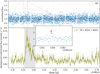 |
Fig. 1 Time series observation of TIC 277 with XMM-Newton. Top panel: XMM-Newton Optical Monitor light curve. Bottom panel: background-subtracted XMM-Newton X-ray light curve using the flux in the entire 0.2–10 keV range (PN, MOS1, and MOS2 combined). The gray shaded portion defines the flare-only subset of the observations (see Sec. 3.1 and Table 2). The inset shows the marginal OM flare; the flare data points are marked with red crosses. |
3.2 Light curve de-trending and flare finding: TESS
We used AltaiPony (Ilin 2021) to de-trend the Pre-search Data Conditioning Simple Aperture Photometry (PDC-SAP) light curves (Fig. 2) using the de-trending function custom_detrending3, detailed in Ilin & Poppenhaeger (2022). The procedure begins with a third-order spline fitting of coarse trends, followed by iterative sine fitting to remove rotational modulation, and two Savitzky-Golay filters (Savitzky & Golay 1964) with a 6 h and 3 h window, respectively, to remove aperiodic short-term trends, while masking potential flare candidates in each step. The masking takes three steps each time. First, all outliers above >2.5σ are masked. Second, to mask the flare decay, we append the six-fold number of data points masked in the first step to the mask. Third, three adjacent data points before and after the expanded mask are added to the mask.
In the de-trended light curves, we searched for flare candidates as at least three consecutive >3σ outliers above the noise level. Here the noise level is defined as the rolling standard deviation of the de-trended light curve flux within a 2 h window, filling in the noise level inside the previously masked areas with the mean of the noise levels adjacent to the mask. To the series of outliers we kept appending data points to the flare candidate until a data point fell below 2σ.
3.3 Light curve de-trending and flare finding: Optical monitor
For the OM data, we performed a simplified analysis in order to identify flare candidates. The photometric noise in the OM data is much higher than in the TESS light curves, so that the rotational modulation is drowned out. We therefore adopted the median value of each light curve, and searched for series of at least three consecutive positive outliers 3σ above the median. We found one candidate with three data points, shown in the inset in Fig. 1. We call this flare candidate marginal because it only barely passes the threshold. The candidate has a relative amplitude of 1.22, larger than any flare detected in the TESS data, but is also much more impulsive, lasting less than a minute, below the 2 min resolution of TESS. While the evidence for this event from the OM alone is weak, its timing of 12 min before the peak of an X-ray flare lends credibility to this detection (see Sec. 4.2).
3.4 EPIC flare detection
In the EPIC light curve, we applied the same approach to finding flares as for OM (Sec. 3.3) because we also did not find any rotational modulation in EPIC. We found one flaring event that stood out. In addition to the data points 3σ or more above the median level, we counted several data points toward the flare before and after to make sure that flaring and quiescent portions of the light curve were clearly separated (see shaded region in Fig. 1).
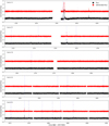 |
Fig. 2 Normalized TESS light curves. The black and red dots show the light curve with and without rotational variability and trends, respectively. The blue vertical lines mark the start times of flare candidates in Table 3. The de-trended light curve is offset by 0.2 for better visibility. The large rotationally modulated flare, localized at about 81° latitude presented by Ilin et al. (2021a), appears in the second half of the top panel (Sector 12). |
3.5 Flare energies: TESS, OM, and EPIC
The OM data contain one marginal flare that we interpret as being associated with the large X-ray flare shortly after (inset in Fig. 1). In the TESS light curves, we found a total of 18 flares. To assess the flaring activity of TIC 277, we computed the bolometric energies for both the OM and the TESS flares.
For the OM flare we used the median flux of the light curve as the quiescent flux F0, against which we measured the equivalent duration (ED) of the flare (i.e., the flare flux Fflare divided by F0, integrated over the flare duration; Gershberg 1972):
![Mathematical equation: $\[\mathrm{ED}=\int \mathrm{d} t \frac{F_{\text {flare }}(t)}{F_0}.\]$](/articles/aa/full_html/2024/07/aa49541-24/aa49541-24-eq3.png) (1)
(1)
We then converted the ED to flare energy using the bolometric flare energy following the procedure in Shibayama et al. (2013). We used the throughput curve for the white light filter scaled to unity at the peak of transmission as an optimistic response curve RλOM, given that the degradation of this filter’s response is poorly constrained4. From this, we extracted a ratio fOM of stellar to flare flux of 1.4 × 10⁻⁴ for a 10 000 K blackbody flare:
![Mathematical equation: $\[f_{\mathrm{OM}}=\frac{\int R_{\lambda, \mathrm{OM}} B_{\lambda\left(T_{\mathrm{eff}}\right)} \mathrm{d} \lambda}{\int R_{\lambda, \mathrm{OM}} B_{\lambda\left(T_{\text {flare }}\right)} \mathrm{d} \lambda}.\]$](/articles/aa/full_html/2024/07/aa49541-24/aa49541-24-eq4.png) (2)
(2)
A flare temperature of Tflare = 10000 K is a typical approximation for energetic M dwarf flares (Kowalski et al. 2013; Howard et al. 2020), but deviations toward both hotter and cooler temperatures are known, which further increases the uncertainty on our energy estimate (Kowalski 2024, and references therein). With the ratio fOM, we can calculate the bolometric flare energy as
![Mathematical equation: $\[E_{\text {flare }}=\mathrm{ED} \cdot \pi R^2 \cdot \sigma_{\mathrm{B}} T_{\mathrm{eff}}^4 \cdot f_{\mathrm{OM}},\]$](/articles/aa/full_html/2024/07/aa49541-24/aa49541-24-eq5.png) (3)
(3)
where σB is the Stefan–Boltzmann constant. We note that due to the optimistic response curve assumption, the resulting Eflare is likely higher in reality.
Analogously to Eq. (2) for the OM flare, we used the TESS response curve to obtain a flux ratio fTESS of 6.3 × 10⁻³ in the optical filter of TESS, and convert ED to bolometric flare energy using Eq. (3). In addition to the ED, AltaiPony also yields the start and end time, defined as the first and last data point above the flare detection criterion defined in Sec. 2.2, and relative amplitude a, for each flare.
For the X-ray flare energy, we multiply flare duration Δt, that is, the difference between start and end time, by the flare luminosity in the EPIC data. The flare luminosity is equal to the difference between the quiescent and flaring X-ray luminosities in the 0.2–2.0 keV band:
![Mathematical equation: $\[E_{X, \text { flare }}=\left(L_{X, \text {flaring}}-L_{X, \text {quiescent}}\right) \cdot \Delta t \text {. }\]$](/articles/aa/full_html/2024/07/aa49541-24/aa49541-24-eq6.png) (4)
(4)
3.6 Flare loop sizes and magnetic field strengths
Because we lack spatial resolution of the stellar disk, we cannot directly measure the flare loop sizes and magnetic field strengths from either X-ray or optical observations. However, we can apply scaling relations based on solar observations (Shibata & Yokoyama 2002; Namekata et al. 2017b) that use X-ray and optical flare diagnostics as proxies. Shibata & Yokoyama (2002) derived scaling relations for the magnetic field strength and loop size from solar soft X-ray observations (their Eqs. (7a) and (7b)):
![Mathematical equation: $\[B=50\left(\frac{\mathrm{EM}}{10^{48} \mathrm{~cm}^{-3}}\right)^{-0.2}\left(\frac{n_0}{10^9 \mathrm{~cm}^{-3}}\right)^{0.3}\left(\frac{T}{10^7 \mathrm{~K}}\right)^{1.7}(\mathrm{G}),\]$](/articles/aa/full_html/2024/07/aa49541-24/aa49541-24-eq7.png) (5)
(5)
![Mathematical equation: $\[L=10^9\left(\frac{\mathrm{EM}}{10^{48} \mathrm{~cm}^{-3}}\right)^{0.6}\left(\frac{n_0}{10^9 \mathrm{~cm}^{-3}}\right)^{-0.4}\left(\frac{T}{10^7 \mathrm{~K}}\right)^{-1.6}(\mathrm{~cm}).\]$](/articles/aa/full_html/2024/07/aa49541-24/aa49541-24-eq8.png) (6)
(6)
We also follow Maehara et al. (2021), who estimate the magnetic field strengths and flaring loop sizes for the OM and TESS flares based on the relation between flare e-folding time τ and bolometric energy Eflare derived from the magnetic reconnection model, and calibrated on solar flares in Namekata et al. (2017b), who themselves use the scaling relations in Shibata & Yokoyama (2002). Namekata et al. (2017b) argue that the e-folding time τ is similar to the magnetic field reconnection time, and that the flare energy Eflare is similar to the magnetic energy stored in the active region where the flare occurs. Using their Eqs. (9) and (10), we obtain
![Mathematical equation: $\[\tau=3.5\left(\frac{E_{\text {flare }}}{1.5 \times 10^{30} \mathrm{~erg}}\right)^{1 / 3}\left(\frac{B}{57 \mathrm{~G}}\right)^{-5 / 3}(\mathrm{~min}).\]$](/articles/aa/full_html/2024/07/aa49541-24/aa49541-24-eq9.png) (7)
(7)
Using the approximation that the flare energy is proportional to the magnetic energy stored in the flaring volume (i.e., Eflare ∝ B2L3; Shibata et al. 2013), we can rephrase the τ − Eflare relation in Eq. (7) in terms of the size of the flaring region, which should be on the order of the loop size:
![Mathematical equation: $\[\tau=3.5\left(\frac{E_{\text {flare }}}{1.5 \times 10^{30} \mathrm{~erg}}\right)^{-1 / 2}\left(\frac{L}{2.4 \times 10^9 \mathrm{~cm}}\right)^{-5 / 2}(\mathrm{~min}).\]$](/articles/aa/full_html/2024/07/aa49541-24/aa49541-24-eq10.png) (8)
(8)
4 Results
In this work, we use the XMM-Newton and TESS observations to constrain the coronal and flaring properties of TIC 277. We derive its coronal temperature and luminosity from the EPIC spectrum (Sec. 4.1). We also measure the flare energies in X-rays from the EPIC instruments, and in optical from the OM, and compare them to the flare frequency distribution obtained from the 18 detected flares in TESS (Sec. 4.2). Finally, we estimate the flaring loop sizes and magnetic field strengths of the XMM-Newton and TESS flares using scaling relations based on solar observations (Sec. 4.3).
4.1 Coronal temperature and luminosity
From the XMM-Newton EPIC spectra, we measured the coronal properties of TIC 277 in both its quiescent, and flaring states (Table 2). The resulting fit for the full data set (Fig. 3) consists of a cooler and a hotter component of about ![Mathematical equation: $\[3.3_{-0.4}^{+0.3}\]$](/articles/aa/full_html/2024/07/aa49541-24/aa49541-24-eq11.png) MK and
MK and ![Mathematical equation: $\[13.1_{-1.4}^{+2.0}\]$](/articles/aa/full_html/2024/07/aa49541-24/aa49541-24-eq12.png) MK, respectively. Assuming these temperatures for the prior distribution, we also fitted 2T VAPEC models to the flaring and quiescent portions of the observations separately. The coronal temperatures did not change significantly using either subset. However, the emission measure weighted mean temperature Tmean changed from 6.5 MK in the quiescent spectrum to 11.3 MK in the flaring spectrum, when the hot component became dominant during the flare. From the quiescent PN spectra, we then also calculated the X-ray flux of FX =(6.3 ± 0.4) × 10−14 erg cm−2s−1 and luminosity LX =(4.56 ± 0.62) × 1026 erg s−1 in the soft 0.2–2.0 keV band. We note that not using the full set of observations as the prior resulted in an unconstrained hot coronal component during the flare, which could be due to a lack of X-ray flux above 5 keV.
MK, respectively. Assuming these temperatures for the prior distribution, we also fitted 2T VAPEC models to the flaring and quiescent portions of the observations separately. The coronal temperatures did not change significantly using either subset. However, the emission measure weighted mean temperature Tmean changed from 6.5 MK in the quiescent spectrum to 11.3 MK in the flaring spectrum, when the hot component became dominant during the flare. From the quiescent PN spectra, we then also calculated the X-ray flux of FX =(6.3 ± 0.4) × 10−14 erg cm−2s−1 and luminosity LX =(4.56 ± 0.62) × 1026 erg s−1 in the soft 0.2–2.0 keV band. We note that not using the full set of observations as the prior resulted in an unconstrained hot coronal component during the flare, which could be due to a lack of X-ray flux above 5 keV.
4.2 Flares
In TESS, we found a total of 18 flares in the five sectors or, equivalently, 125 days of observing at 2 min cadence. We fit the flare frequency distribution (FFD) with a power law of the form
![Mathematical equation: $\[f(E) \mathrm{d} E=\beta \cdot E^{-\alpha} \mathrm{d} E,\]$](/articles/aa/full_html/2024/07/aa49541-24/aa49541-24-eq13.png) (9)
(9)
following the procedure in Ilin et al. (2021b), implemented as FFD.fit_powerlaw using the mcmc argument in AltaiPony (Ilin 2021), which uses the posterior distribution derived in Wheatland (2004), and samples the posterior distribution with the emcee package (Foreman-Mackey et al. 2013).
The FFD power law fit converged after 13 500 steps on a slope ![Mathematical equation: $\[\alpha=-1.86_{-0.21}^{+0.18}\]$](/articles/aa/full_html/2024/07/aa49541-24/aa49541-24-eq26.png) . The frequency R31.5, which is the frequency of flares per day above log10 Eflare [erg] = 31.5, is log10 R31.5 =−0.94 d−1. The slope is typical of other flaring stars, regardless of spectral type and rotation period (see, e.g., Fig. 13 of Ilin et al. 2021b). The frequency R31.5 is typical of flaring M dwarfs, including late M dwarfs in the saturated activity regime, where R31.5 becomes independent of rotation period (Medina et al. 2020; Murray et al. 2022).
. The frequency R31.5, which is the frequency of flares per day above log10 Eflare [erg] = 31.5, is log10 R31.5 =−0.94 d−1. The slope is typical of other flaring stars, regardless of spectral type and rotation period (see, e.g., Fig. 13 of Ilin et al. 2021b). The frequency R31.5 is typical of flaring M dwarfs, including late M dwarfs in the saturated activity regime, where R31.5 becomes independent of rotation period (Medina et al. 2020; Murray et al. 2022).
For the X-ray flare in Fig. 1, we obtain a total energy of (4.7 ± 2.2) × 1030 erg in the 0.2–2.0 keV band by inserting the quiescent and flaring luminosities (Table 2), and Δt =4.5 ks (see Fig. 1) into Eq. (4). With Eq. (2), we find an energy of (3.7 ± 0.7) × 1030 erg for the corresponding OM flare. We use the 36 ks observing baseline of XMM-Newton to calculate a flare rate in OM based on the detection of this single event. Figure 4 illustrates that the OM flare rate is roughly consistent, if slightly higher, than the extension of the TESS FFD to lower energies. Assuming a 1:1 correspondence between optical and X-ray flares, about one flare per day with energies on the order of the observed event or above can therefore be expected in future X-ray observations of TIC 277, based on the TESS FFD. However, usually, not all optical flares have X-ray counterparts (Paudel et al. 2021), and those that do show order of magnitude variable ratios of optical versus X-ray energy (Guarcello et al. 2019; Kuznetsov & Kolotkov 2021; Joseph et al. 2024), implying that XMM-Newton flare rates in the range 0.1–10 day−1 are possible for TIC 277.
The (marginal) OM flare precedes the soft X-ray flare, which is typical of flares that show the Neupert effect (Neupert 1968). This timing suggests that we observed the same event at two different wavelengths. The Neupert criterion states that the peak of the nonthermal radio emission should coincide with the moment of fastest rise in the thermal soft X-ray emission. As radio monitoring is rarely available for stellar flare observations, blue-optical and near ultraviolet are sometimes used as proxies (Hawley et al. 1995, 2003). Many M dwarf flares follow the Neupert effect (e.g., Guedel et al. 1996; Stelzer et al. 2022a); others deviate from it (Hawley et al. 1995; Osten et al. 2005), either not showing the time delay at all (non-Neupert flares), or a time delay inconsistent with the Neupert criterion (quasi-Neupert flares; Tristan et al. 2023). In our data the peak of the blue-optical flare peak precedes the X-ray peak by 12 min, overlapping with the fast rise phase of the soft X-ray flare. This suggests that this flare is a true Neupert flare, but the time resolution is too low to discriminate this instance from a potential quasi-Neupert case. Finally, we note that the X-ray flare light curve follows the typical fast-rise exponential decay shape, and is therefore unlikely to be eclipsed by the star despite its fast rotation.
XSPEC fits to EPIC spectra for different subsets of observations.
 |
Fig. 3 Time-averaged XMM-Newton EPIC spectra. The top panel shows the spectra taken with the different EPIC instruments (data points with error bars) together with the best-fit two-temperature VAPEC model with Fe/O = 0.6 for the full data set (solid lines). The bottom panel shows the residuals to the fit. |
Flares detected with TESS.
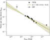 |
Fig. 4 Cumulative flare frequency distribution of TESS flares (black dots), with a power law fit (green line) and uncertainties (dotted lines). The rate of OM flares (gray square) is calculated from the observing baseline of XMM-Newton. The flare energies are corrected for the pass bands of TESS and OM, i.e., given as bolometric flare energies (see Sec. 3.5). |
4.3 Flare loop sizes and magnetic field strengths
Based on the flare parameters obtained from EPIC, OM, and TESS, we estimated the flaring loop magnetic field strength B and loop size L using the scaling relations introduced in Sec. 3.6. For the EPIC flare, we use Eq. (5) to obtain the magnetic field strength and Eq. (6) to derive the loop size from the flaring EM and Thot, assuming flaring coronal densities n0 = 1011, 1012, and 1013 cm−3 (Table 4). The lower two values are typical of main-sequence M dwarfs with measured coronal species abundances (Güdel 2004; Liefke et al. 2010), and the latter only found in accreting T Tauri stars (Stelzer & Schmitt 2004).
For the optical OM and TESS flares, we follow Namekata et al. (2017b) and Maehara et al. (2021), and use Eqs. (7) and (8) to overlay the relation between e-folding time τ and bolometric flare energy Eflare with a range of possible values for B and L. We fit an exponential function to all TESS flares and the OM flare, fixing the amplitude of the exponential decay to 5% within the peak amplitude of the flare, and the start of the exponential decay to within 5 min or 20 s of the peak time of the flare in TESS and OM, respectively. Figure 5 shows that τ and Eflare are correlated. The TESS flares appear compatible with magnetic field strengths between 30 G and 250 G, similar to other active M dwarfs (Karmakar et al. 2021; Notsu et al. 2024). Their loop sizes are between 3 × 109 cm and 2 × 1010 cm, which is roughly 0.3–2 R*, except for the energetic high-latitude flare, for which we estimated the energy and e-folding time from the underlying, rotationally unmodulated flare (Ilin 2021), and that yields a loop size of around 5 × 1010 cm, or 5 R*. The OM flare extends the trend of the TESS flares to lower energies with a magnetic field strength of 250 G and a loop size of 109 cm, or 0.1 R*. This result is compatible with the results for the EPIC flare for loop number densities between 1011 cm−3 and 1012 cm−3 (see Table 4).
All scaling laws used here make assumptions about the state of the corona (e.g., the loop electron density; Shibata & Yokoyama 2002) and the flare model (e.g., the magnetic reconnection model; Namekata et al. 2017b). It is encouraging that the XMM-Newton flare yields similar results for both EPIC and OM data, but the results for the TESS flares should be interpreted cautiously and differentially with other flare studies with the same method (Maehara et al. 2021) rather than as absolute values.
Magnetic field strength B and loop size L of the EPIC flare.
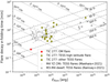 |
Fig. 5 Flare decay e-folding time τ vs. flare energy Eflare for the OM flare, and the TESS flares. The dashed and dotted lines show the τ−Eflare relations from Eqs. (7) and (8) for different loop magnetic field strengths and loop sizes, respectively. For comparison, we show the TESS flares of the active M4 dwarf YZ CMi (Maehara et al. 2021) and a range of nearby M dwarfs from TESS with large flares (Ramsay et al. 2021). |
5 Discussion
TIC 277’s spectral type and rotation place it in the middle of the transition from star to brown dwarf. Our findings indicate that TIC 277’s coronal temperature (Sec. 5.1), flaring activity (Sec. 5.2), and flare loop sizes and magnetic fields (Sec. 5.3) are typical of saturated fully convective M dwarf stars. However, TIC 277 is rotating rapidly, even for the typically fast-rotating late M dwarfs (Medina et al. 2022). This combination could lead to an unusual manifestation of the stellar dynamo that produces high-latitude flares (Weber & Browning 2016; Weber et al. 2023). TIC 277 is fainter in X-ray by about an order of magnitude than earlier-type M dwarfs on the canonical saturated branch (Magaudda et al. 2022b), which, in combination with the detection of a high-latitude flare, may be an indication of polar updraft migration that is suspected to occur in rapid rotators (Sec. 5.4).
5.1 Coronal temperature
The coronae of low-mass stars are not uniform. Magnetic structures create a range of temperatures, starting at about 1 MK and increasing to 30 MK in flares in the heterogeneous solar corona (Vaiana & Rosner 1978). Stellar point source X-ray observations are a superposition of various temperatures and densities. The resolution of different temperature components depends on the apparent brightness and integration time of the spectrum. Nearby stars like Proxima Cen can be modeled with a range of temperatures (e.g., Güdel et al. 2004; Drake et al. 2020), while it is often possible to capture only a single or a few dominant temperatures in fainter objects.
We find that the XMM-Newton observations of the quiescent corona of TIC 277 are best described by two temperature components, similar to many other active M dwarfs. Assuming that TIC 277 produces flares below the detection threshold of XMM-Newton that contribute to the temperature makeup of the quiescent corona, the presence of a second, hotter component is consistent with the standard picture for stellar flares (Wargelin et al. 2008; Robrade et al. 2010; Behr et al. 2023; Magaudda et al. 2022b). Both the cooler and the hotter component represent thermal radiation from hot plasma that evaporates from the chromosphere into the corona. The dominance of the hot component during the flare combined with the observed Neupert effect (see Sec. 4.2) is evidence that this component is driven by particles precipitating downward during flares that then heat the chromosphere to high temperatures, and cause evaporation into the coronal flaring loops. In addition, quiescent heating through other sources under debate, such as Alfvén waves or nanoflares (Benz 2016), are present at a constant level represented by the cool component.
The range of 6.5–11 MK for the emission measure weighted temperature of TIC 277 places it squarely in the saturated regime with other mid M dwarfs down to spectral type M6 (Wright et al. 2018; Magaudda et al. 2020; Stelzer et al. 2022b; Robrade & Schmitt 2005; Raassen et al. 2003; Paudel et al. 2021; Foster et al. 2020). Flares on the slowly rotating Proxima Cen (M5.5, Prot = 83 days, Anglada-Escudé et al. 2016), appear with a range of temperatures at 2–3 MK and 10–20 MK (Güdel et al. 2004; Fuhrmeister et al. 2011, 2022; Howard et al. 2022). Its X-ray luminosity (Haisch et al. 1990) and flaring activity (Howard et al. 2018; Medina et al. 2020) place it in the transition region between saturated and unsaturated regimes. Only at rotation periods beyond 100 days can stellar activity decrease to yield coronal temperatures <2 MK in M3–M6 dwarfs (Wright et al. 2018; Foster et al. 2020).
There are only a few late M dwarfs beyond spectral type M6 with a spectrally resolved corona. Their intrinsic faintness and gradual decline in coronal emission toward the brown dwarf regime make them hard to detect (Berger et al. 2010; Cook et al. 2014; Stelzer et al. 2022b). One example is NLTT 33370 AB. This M7 binary with a rotation period of about 3.8 h (close to the TIC 277 roation of 4.56 h, and of the same spectral type) is composed of a 3.1 MK and 14 MK component (Williams et al. 2015). Another is TRAPPIST-1 (M8, Prot = 3.3 days, Luger et al. 2017). Its corona appears cooler, with a 1.74 MK and a 9.6 MK component (Wheatley et al. 2017), and an emission measure weighted temperature of 5.36 MK (Brown et al. 2023).
Bearing in mind the relatively low two-temperature resolution of TIC 277’s X-ray spectrum and the dearth of X-ray spectra for stars at the bottom of the main sequence, it shows a coronal temperature make-up common for mid-to-late M dwarfs in the saturated activity regime, which it will possibly keep for gigayears until it spins down to very low rotation rates (Medina et al. 2022; Engle & Guinan 2023).
5.2 Flaring activity
TIC 277’s flare rate is consistent with that of other saturated fully convective dwarfs (Medina et al. 2020; Murray et al. 2022), and so is the energy distribution with a power law slope of ![Mathematical equation: $\[-1.86_{-0.21}^{+0.18}\]$](/articles/aa/full_html/2024/07/aa49541-24/aa49541-24-eq27.png) . It is comparable to TRAPPIST-1’s flaring behavior (Paudel et al. 2018), which has been investigated for its effects on the seven terrestrial planets in its orbit.
. It is comparable to TRAPPIST-1’s flaring behavior (Paudel et al. 2018), which has been investigated for its effects on the seven terrestrial planets in its orbit.
TIC 277’s rapid rotation and UV flux hint at a younger age than TRAPPIST-1, which is likely a field star (Burgasser & Mamajek 2017; Birky et al. 2021; Gonzales et al. 2019). TIC 277 has not been attributed to any moving group to date (Schneider & Shkolnik 2018), and the number of late M dwarfs with an independently measured age and rotation is too small to infer age based on rotation alone (Engle & Guinan 2023). Interpreting the upcoming observations of TRAPPIST-1 e, one of the rocky planets in the habitable zone of the system, with the James Webb Space Telescope will most likely involve its activity history. Studies of its younger counterparts, late M dwarfs like TIC 277, are required to empirically constrain cumulative effects of atmospheric forcing of planets. If its energetic flares commonly occur at high latitudes (Ilin et al. 2021a), future models of energetic particle exposure of habitable zone planets may have to include age dependent latitudes of particle eruption to reproduce observations.
5.3 Flare loop sizes and magnetic field strength
The XMM-Newton flare emitted an energy of (4.7 ± 2.2) × 1030 erg, comparable to that of energetic solar flares, and the loop size derived from both EPIC and OM is within their range of 108−1010 cm (Aschwanden et al. 2015; Namekata et al. 2017a). The TESS flares show loop sizes between 0.3 and 5 R*, consistent with M dwarf flares with similar energies (Schmitt & Liefke 2002; Stelzer et al. 2006, 2022a; Karmakar et al. 2021; Ramsay et al. 2021; Notsu et al. 2024; Guarcello et al. 2019; Doyle et al. 2022).
The XMM-Newton flare observations suggest a magnetic field strength of around 150–250 G from both the EPIC and OM data, stronger than the fields of solar coronal loops which are typically below 100 G (Namekata et al. 2017a). However, solar flares show higher field strengths up to 350 G in high spatial resolution spectropolarimetric and radio observations, suggesting that lower resolution underestimates the field strength (Kuridze et al. 2019; Yu et al. 2020). Since the scaling relations used in this work are based on the older solar flare measurements, the estimates we derived may be too low by up to a factor of five (Kuridze et al. 2019).
In a differential comparison, the magnetic field strengths of 30–250 G of the TESS flares follow the trend of other activity saturated early to mid-M dwarfs (Fig. 5, Ramsay et al. 2021; Maehara et al. 2021). For late M dwarfs like TIC 277, only a few estimates of flare loop sizes and field strengths exist in the literature (Schmitt & Liefke 2002; Stelzer et al. 2006) that are consistent with our results, but there are no such estimates for flare energies below 1031 erg.
Overall, TIC 277’s flare loop sizes and field strengths appear consistent with those of active M dwarfs of similar energies. However, we cannot say if other late M dwarfs behave similarly in the low-energy range of the XMM-Newton flare. Reports of late M dwarf flares at energies below 1031 erg exist in the literature (e.g., Paudel et al. 2018; Howard et al. 2022; Petrucci et al. 2024), but we leave the worthwhile exercise of estimating their loop lengths and field strengths to future work.
5.4 X-ray luminosity
TIC 277’s coronal luminosity relative to bolometric luminosity of LX/Lbol =(0.9 ± 0.1) × 10−4 in quiescence is about an order of magnitude lower than the canonical LX /Lbol ~ 10−3 average in the saturated regime of partly and fully convective M dwarfs (Wright et al. 2011; Wright & Drake 2016; Wright et al. 2018). However, recent studies limited to low-mass M dwarfs (M* ~ 0.15–0.3 M⊙) show that the saturation level is near LX/Lbol ≈ 10−3.5 (Magaudda et al. 2022a) On the contrary, in a sample of late M dwarfs investigated with eROSITA, LX/Lbol appears to increase toward later spectral types (Stelzer et al. 2022b). However, these detections are likely to be attributed to flares, and thus are not representative for the average X-ray emission level of late M dwarfs. While TIC 277 appears at the lower end of the LX/Lbol distribution with respect to that sample and to similar previous work (Stelzer et al. 2012; Cook et al. 2014; De Luca et al. 2020; Williams et al. 2014; Berger et al. 2008), the latest eROSITA study on a well-defined sample of nearby late M to early L dwarfs has shown that rapidly rotating late M dwarfs display a broad range of X-ray luminosities centered around LX/Lbol ≈ 10−4 placing TIC 277 in the center of their distribution (Magaudda et al. 2024).
At late M spectral types, a decline in coronal activity is expected as the magnetosphere transitions from stellar to planetary (Pineda et al. 2017). A decline in X-ray activity is expected as a result of decreasing efficiency of coronal heating (e.g., Mohanty et al. 2002; Williams et al. 2014). However, the flaring activity and coronal temperature of TIC 277 and similar late M dwarfs show that the corona is still capable of producing flares. For the specific case of the rapidly rotating TIC 277, polar updraft migration (Stepień et al. 2001) could at the same time explain the decline in X-ray luminosity and the occurrence of a high-latitude flare observed by TESS. Polar updraft migration implies that at high rotation rates, flux emergence becomes more efficient near the poles than at the equator (Yadav et al. 2015; Weber & Browning 2016) producing flares there, but draining the equatorial regions of magnetic flux required to produce a corona at low latitudes. As a result, the X-ray luminosity diminishes. Since TIC 277 is seen nearly equator-on (Table 1), polar updraft migration could explain its fainter corona. Considering the high-latitude flare, viewing geometry, star-like flaring behavior, and star-like coronal temperatures together, we suggest this scenario as an alternative to the brown dwarf transition explanation that invokes a diminishing corona due to the overall cooler, more neutral atmosphere.
6 Summary and conclusions
We investigated whether TIC 277, a rapidly rotating M7 dwarf that exhibited a flare localized at 81° latitude, shows coronal or flaring properties that could explain the occurrence of this flare so close to the rotational pole. We obtained 36 ks of EPIC and OM observations with XMM-Newton, and studied the five sectors of red-optical 27-day light curves provided by TESS. We found a mean quiescent coronal temperature of 6.5 MK, and a flaring rate f(> log10 Eflare,bol = 31.5 erg) ≈−0.94 d−1 with an energy distribution slope of ![Mathematical equation: $\[-1.86_{-0.21}^{+0.18}\]$](/articles/aa/full_html/2024/07/aa49541-24/aa49541-24-eq28.png) , all typical of M dwarfs in the saturated regime. We also detected a simultaneous X-ray and optical flare with an energy of (4.7 ± 2.2) × 1030 erg in the 0.2–2 keV band, and bolometric energy of (3.7 ± 0.7) × 1030 erg from the OM observations. In combination with the 18 detected TESS flares, we estimate that X-ray flares on TIC 277 can be observed with XMM-Newton about once a day. We used scaling relations to estimate the loop sizes and magnetic fields of the flares, and found mutually consistent fields of 30–250 G and loop lengths ranging from 0.1R* for the low-energy XMM-Newton flare to 5R* for the giant high-latitude TESS flare. Similar values have been reported for activity saturated M dwarfs in the literature, except for the XXMM-Newton flare, which extends the duration-energy relation to more impulsive and less energetic flares. An indication of an unusual corona stems from its X-ray luminosity relative to bolometric luminosity LX/Lbol =(0.9 ± 0.1) × 10−4. It is an order of magnitude lower than the canonical value for saturated activity M dwarfs, but representative of late M dwarfs of spectral type M7 and later. TIC 277 is an extremely rapid rotator with a rotation period of only 4.56 h. The detected high-latitude flare in TESS (Ilin et al. 2021a) may hence be a product of high-latitude flux emergence driven by its fast rotation (Weber & Browning 2016; Weber et al. 2017). The low X-ray luminosity and the high-latitude flare taken together with the star’s fast rotation, saturated flaring activity, and equator-on viewing angle could be explained by polar updraft migration, which suppresses coronal emission in equatorial regions and confines the corona and flaring regions to near-polar latitudes (Stepień et al. 2001).
, all typical of M dwarfs in the saturated regime. We also detected a simultaneous X-ray and optical flare with an energy of (4.7 ± 2.2) × 1030 erg in the 0.2–2 keV band, and bolometric energy of (3.7 ± 0.7) × 1030 erg from the OM observations. In combination with the 18 detected TESS flares, we estimate that X-ray flares on TIC 277 can be observed with XMM-Newton about once a day. We used scaling relations to estimate the loop sizes and magnetic fields of the flares, and found mutually consistent fields of 30–250 G and loop lengths ranging from 0.1R* for the low-energy XMM-Newton flare to 5R* for the giant high-latitude TESS flare. Similar values have been reported for activity saturated M dwarfs in the literature, except for the XXMM-Newton flare, which extends the duration-energy relation to more impulsive and less energetic flares. An indication of an unusual corona stems from its X-ray luminosity relative to bolometric luminosity LX/Lbol =(0.9 ± 0.1) × 10−4. It is an order of magnitude lower than the canonical value for saturated activity M dwarfs, but representative of late M dwarfs of spectral type M7 and later. TIC 277 is an extremely rapid rotator with a rotation period of only 4.56 h. The detected high-latitude flare in TESS (Ilin et al. 2021a) may hence be a product of high-latitude flux emergence driven by its fast rotation (Weber & Browning 2016; Weber et al. 2017). The low X-ray luminosity and the high-latitude flare taken together with the star’s fast rotation, saturated flaring activity, and equator-on viewing angle could be explained by polar updraft migration, which suppresses coronal emission in equatorial regions and confines the corona and flaring regions to near-polar latitudes (Stepień et al. 2001).
Overall, less than ten flare latitudes on stars other than the Sun are known to date (Wolter et al. 2008; Ilin et al. 2021a; Johnson et al. 2021). Localization of more flares on the surfaces of a broader range of stars will allow us to resolve whether polar updraft migration indeed occurs in these stars.
Acknowledgements
E.I. and D.D. acknowledge funding from the Deutsche Luft- und Raumfahrtgesellschaft (FKZ 50 OR 2209, project X-ray Loops). K.P. acknowledges funding from the German Leibniz-Gemeinschaft under project number P67/2018. This work is based on observations obtained with XMM-Newton, an ESA science mission with instruments and contributions directly funded by ESA Member States and NASA. This paper includes data collected by the TESS mission. Funding for the TESS mission is provided by the NASA’s Science Mission Directorate. This work made use of the open source python software packages lightkurve (Lightkurve Collaboration 2018), astropy (Astropy Collaboration 2013), numpy (Harris et al. 2020), pandas (Reback et al. 2022), matplotlib (Hunter 2007), emcee (Foreman-Mackey et al. 2013), scipy (McKinney 2010), and altaipony (Ilin 2021). This work has made use of data from the European Space Agency (ESA) mission Gaia (https://www.cosmos.esa.int/gaia), processed by the Gaia Data Processing and Analysis Consortium (DPAC, https://www.cosmos.esa.int/web/gaia/dpac/consortium). Funding for the DPAC has been provided by national institutions, in particular the institutions participating in the Gaia Multilateral Agreement.
Data availability. All data used in this study are publicly available in their respective archives: the Mikulski Archive for Space Telescopes (MAST, https://mast.stsci.edu/portal/Mashup/Clients/Mast/Portal.html) for TESS, and the XMM-Newton Science Archive (https://www.cosmos.esa.int/web/xmm-newton/xsa). The scripts used to produce the figures in the git repository on GitHub are available at github.com/ekaterinailin/xmm_for_tic277. The data analysis scripts can be found under github.com/ekaterinailin/tic277.
References
- Airapetian, V. S., Barnes, R., Cohen, O., et al. 2020, Int. J. Astrobiol., 19, 136 [NASA ADS] [CrossRef] [Google Scholar]
- Anglada-Escudé, G., Amado, P. J., Barnes, J., et al. 2016, Nature, 536, 437 [Google Scholar]
- Arnaud, K. A. 1996, Astronomical Data Analysis Software and Systems V, ASP Conf. Ser., 101, 17 [NASA ADS] [Google Scholar]
- Aschwanden, M. J., Boerner, P., Ryan, D., et al. 2015, ApJ, 802, 53 [Google Scholar]
- Astropy Collaboration (Robitaille, T. P., et al.) 2013, A&A, 558, A33 [NASA ADS] [CrossRef] [EDP Sciences] [Google Scholar]
- Audard, M., Osten, R. A., Brown, A., et al. 2007, A&A, 471, L63 [NASA ADS] [CrossRef] [EDP Sciences] [Google Scholar]
- Bailer-Jones, C. A. L., Rybizki, J., Fouesneau, M., Mantelet, G., & Andrae, R. 2018, AJ, 156, 58 [Google Scholar]
- Behr, P. R., France, K., Brown, A., et al. 2023, AJ, 166, 35 [NASA ADS] [CrossRef] [Google Scholar]
- Benz, A. O. 2016, Liv. Rev. Sol. Phys., 14, 2 [Google Scholar]
- Berger, E., Basri, G., Gizis, J. E., et al. 2008, ApJ, 676, 1307 [NASA ADS] [CrossRef] [Google Scholar]
- Berger, E., Basri, G., Fleming, T. A., et al. 2010, ApJ, 709, 332 [Google Scholar]
- Birky, J., Barnes, R., & Fleming, D. P. 2021, RNAAS, 5, 122 [NASA ADS] [Google Scholar]
- Brown, A., Schneider, P. C., France, K., et al. 2023, AJ, 165, 195 [NASA ADS] [CrossRef] [Google Scholar]
- Burgasser, A. J., & Mamajek, E. E. 2017, ApJ, 845, 110 [Google Scholar]
- Cook, B. A., Williams, P. K. G., & Berger, E. 2014, ApJ, 785, 10 [NASA ADS] [CrossRef] [Google Scholar]
- De Luca, A., Stelzer, B., Burgasser, A. J., et al. 2020, A&A, 634, A13 [NASA ADS] [CrossRef] [EDP Sciences] [Google Scholar]
- do Amaral, L. N. R., Barnes, R., Segura, A., & Luger, R. 2022, ApJ, 928, 12 [NASA ADS] [CrossRef] [Google Scholar]
- Doyle, J. G., Irawati, P., Kolotkov, D. Y., et al. 2022, MNRAS, 514, 5178 [NASA ADS] [CrossRef] [Google Scholar]
- Drake, J. J., Kashyap, V. L., Wargelin, B. J., & Wolk, S. J. 2020, ApJ, 893, 137 [Google Scholar]
- Dressing, C. D., & Charbonneau, D. 2015, ApJ, 807, 45 [Google Scholar]
- Engle, S. G., & Guinan, E. F. 2023, ApJ, 954, L50 [NASA ADS] [CrossRef] [Google Scholar]
- Foreman-Mackey, D., Hogg, D. W., Lang, D., & Goodman, J. 2013, PASP, 125, 306 [Google Scholar]
- Foster, A. R., Ji, L., Smith, R. K., & Brickhouse, N. S. 2012, ApJ, 756, 128 [Google Scholar]
- Foster, G., Poppenhaeger, K., Alvarado-Gómez, J. D., & Schmitt, J. H. M. M. 2020, MNRAS, 497, 1015 [Google Scholar]
- Fuhrmeister, B., Lalitha, S., Poppenhaeger, K., et al. 2011, A&A, 534, A133 [NASA ADS] [CrossRef] [EDP Sciences] [Google Scholar]
- Fuhrmeister, B., Zisik, A., Schneider, P. C., et al. 2022, A&A, 663, A119 [NASA ADS] [CrossRef] [EDP Sciences] [Google Scholar]
- Garraffo, C., Drake, J. J., Cohen, O., Alvarado-Gómez, J. D., & Moschou, S. P. 2017, ApJ, 843, L33 [Google Scholar]
- Gershberg, R. E. 1972, Astrophys. Space Sci., 19, 75 [NASA ADS] [CrossRef] [Google Scholar]
- Gizis, J. E., Burgasser, A. J., Berger, E., et al. 2013, ApJ, 779, 172 [NASA ADS] [CrossRef] [Google Scholar]
- Gonzales, E. C., Faherty, J. K., Gagné, J., et al. 2019, ApJ, 886, 131 [Google Scholar]
- Grevesse, N., & Sauval, A. J. 1998, Space Sci. Rev., 85, 161 [Google Scholar]
- Guarcello, M. G., Micela, G., Sciortino, S., et al. 2019, A&A, 622, A210 [NASA ADS] [CrossRef] [EDP Sciences] [Google Scholar]
- Guedel, M., Benz, A. O., Schmitt, J. H. M. M., & Skinner, S. L. 1996, ApJ, 471, 1002 [NASA ADS] [CrossRef] [Google Scholar]
- Güdel, M. 2004, A&ARv, 12, 71 [CrossRef] [Google Scholar]
- Güdel, M., Audard, M., Reale, F., Skinner, S. L., & Linsky, J. L. 2004, A&A, 416, 713 [NASA ADS] [CrossRef] [EDP Sciences] [Google Scholar]
- Haisch, B. M., Butler, C. J., Foing, B., Rodono, M., & Giampapa, M. S. 1990, A&A, 232, 387 [NASA ADS] [Google Scholar]
- Hardegree-Ullman, K. K., Cushing, M. C., Muirhead, P. S., & Christiansen, J. L. 2019, AJ, 158, 75 [Google Scholar]
- Harris, C. R., Millman, K. J., van der Walt, S. J., et al. 2020, Nature, 585, 357 [NASA ADS] [CrossRef] [Google Scholar]
- Hawley, S. L., Fisher, G. H., Simon, T., et al. 1995, ApJ, 453, 464 [NASA ADS] [CrossRef] [Google Scholar]
- Hawley, S. L., Allred, J. C., Johns-Krull, C. M., et al. 2003, ApJ, 597, 535 [Google Scholar]
- Howard, W. S., Tilley, M. A., Corbett, H., et al. 2018, ApJ, 860, L30 [Google Scholar]
- Howard, W. S., Corbett, H., Law, N. M., et al. 2020, ApJ, 902, 115 [Google Scholar]
- Howard, W. S., MacGregor, M. A., Osten, R., et al. 2022, ApJ, 938, 103 [NASA ADS] [CrossRef] [Google Scholar]
- Hunter, J. D. 2007, Comput. Sci. Eng., 9, 90 [NASA ADS] [CrossRef] [Google Scholar]
- Ilin, E. 2021, J. Open Source Softw., 6, 2845 [NASA ADS] [CrossRef] [Google Scholar]
- Ilin, E., & Poppenhaeger, K. 2022, MNRAS, 513, 4579 [NASA ADS] [CrossRef] [Google Scholar]
- Ilin, E., Poppenhaeger, K., Schmidt, S. J., et al. 2021a, MNRAS, 507, 1723 [CrossRef] [Google Scholar]
- Ilin, E., Schmidt, S. J., Poppenhäger, K., et al. 2021b, A&A, 645, A42 [NASA ADS] [CrossRef] [EDP Sciences] [Google Scholar]
- Johnson, E. N., Czesla, S., Fuhrmeister, B., et al. 2021, A&A, 651, A105 [NASA ADS] [CrossRef] [EDP Sciences] [Google Scholar]
- Johnstone, C. P., Bartel, M., & Güdel, M. 2021, A&A, 649, A96 [EDP Sciences] [Google Scholar]
- Joseph, W. M., Stelzer, B., Magaudda, E., & Vičánek Martínez, T. 2024, arXiv e-prints [arXiv:2401.17287] [Google Scholar]
- Karmakar, S., Naik, S., Pandey, J. C., & Savanov, I. S. 2021, MNRAS, 509, 3247 [NASA ADS] [CrossRef] [Google Scholar]
- Ketzer, L., & Poppenhaeger, K. 2023, MNRAS, 518, 1683 [Google Scholar]
- Kowalski, A. F. 2024, Liv. Rev. Sol. Phys., 21, 1 [NASA ADS] [CrossRef] [Google Scholar]
- Kowalski, A. F., Hawley, S. L., Wisniewski, J. P., et al. 2013, ApJS, 207, 15 [NASA ADS] [CrossRef] [Google Scholar]
- Kuridze, D., Mathioudakis, M., Morgan, H., et al. 2019, ApJ, 874, 126 [Google Scholar]
- Kuznetsov, A. A., & Kolotkov, D. Y. 2021, ApJ, 912, 81 [NASA ADS] [CrossRef] [Google Scholar]
- Lammer, H., Selsis, F., Ribas, I., et al. 2003, ApJ, 598, L121 [Google Scholar]
- Liefke, C., Fuhrmeister, B., & Schmitt, J. H. M. M. 2010, A&A, 514, A94 [NASA ADS] [CrossRef] [EDP Sciences] [Google Scholar]
- Lightkurve Collaboration (Cardoso, J. V. d. M., et al.) 2018, Astrophysics Source Code Library, [record ascl:1812.013] [Google Scholar]
- Luger, R., Sestovic, M., Kruse, E., et al. 2017, Nat. Astron., 1, 0129 [Google Scholar]
- Maehara, H., Notsu, Y., Namekata, K., et al. 2021, PASJ, 73, 44 [NASA ADS] [CrossRef] [Google Scholar]
- Magaudda, E., Stelzer, B., Covey, K. R., et al. 2020, A&A, 638, A20 [NASA ADS] [CrossRef] [EDP Sciences] [Google Scholar]
- Magaudda, E., Stelzer, B., & Raetz, S. 2022a, Astron. Nachr., 343, e20220049 [NASA ADS] [CrossRef] [Google Scholar]
- Magaudda, E., Stelzer, B., Raetz, S., et al. 2022b, A&A, 661, A29 [NASA ADS] [CrossRef] [EDP Sciences] [Google Scholar]
- Magaudda, E., Stelzer, B., Osten, R. A., et al. 2024, A&A, 687, A95 [NASA ADS] [CrossRef] [EDP Sciences] [Google Scholar]
- McKinney, W. 2010, Proceedings of the 9th Python in Science Conference, 56 [CrossRef] [Google Scholar]
- Medina, A. A., Winters, J. G., Irwin, J. M., & Charbonneau, D. 2020, ApJ, 905, 107 [Google Scholar]
- Medina, A. A., Winters, J. G., Irwin, J. M., & Charbonneau, D. 2022, ApJ, 935, 104 [NASA ADS] [CrossRef] [Google Scholar]
- Ment, K., & Charbonneau, D. 2023, AJ, 165, 265 [NASA ADS] [CrossRef] [Google Scholar]
- Mohanty, S., Basri, G., Shu, F., Allard, F., & Chabrier, G. 2002, ApJ, 571, 469 [NASA ADS] [CrossRef] [Google Scholar]
- Mullan, D. J., & Paudel, R. R. 2018, ApJ, 854, 14 [NASA ADS] [CrossRef] [Google Scholar]
- Murray, C. A., Queloz, D., Gillon, M., et al. 2022, MNRAS [Google Scholar]
- Namekata, K., Sakaue, T., Watanabe, K., et al. 2017a, ApJ, 851, 91 [Google Scholar]
- Namekata, K., Sakaue, T., Watanabe, K., Asai, A., & Shibata, K. 2017b, PASJ, 69, 7 [NASA ADS] [CrossRef] [Google Scholar]
- Neupert, W. M. 1968, ApJ, 153, L59 [NASA ADS] [CrossRef] [Google Scholar]
- Notsu, Y., Kowalski, A. F., Maehara, H., et al. 2024, AJ, 961, 189 [NASA ADS] [CrossRef] [Google Scholar]
- Osten, R. A., Hawley, S. L., Allred, J. C., Johns-Krull, C. M., & Roark, C. 2005, ApJ, 621, 398 [Google Scholar]
- Paudel, R. R., Gizis, J. E., Mullan, D. J., et al. 2018, ApJ, 858, 55 [Google Scholar]
- Paudel, R. R., Gizis, J. E., Mullan, D. J., et al. 2020, MNRAS, 494, 5751 [NASA ADS] [CrossRef] [Google Scholar]
- Paudel, R. R., Barclay, T., Schlieder, J. E., et al. 2021, ApJ, 922, 31 [NASA ADS] [CrossRef] [Google Scholar]
- Pecaut, M. J., & Mamajek, E. E. 2013, ApJS, 208, 9 [Google Scholar]
- Petrucci, R. P., Gómez Maqueo Chew, Y., Jofré, E., Segura, A., & Ferrero, L. V. 2024, MNRAS, 527, 8290 [Google Scholar]
- Pineda, J. S., Hallinan, G., & Kao, M. M. 2017, ApJ, 846, 75 [Google Scholar]
- Raassen, A. J. J., Mewe, R., Audard, M., & Güdel, M. 2003, A&A, 411, 509 [NASA ADS] [CrossRef] [EDP Sciences] [Google Scholar]
- Ramsay, G., Kolotkov, D., Doyle, J. G., & Doyle, L. 2021, Sol. Phys., 296, 162 [NASA ADS] [CrossRef] [Google Scholar]
- Reback, J. jbrockmendel, McKinney, W., et al. 2022 https://doi.org/10.5281/zenodo.6408044 [Google Scholar]
- Ricker, G. R., Winn, J. N., Vanderspek, R., et al. 2015, J. Astron. Telescopes Instrum. Syst., 1, 014003 [Google Scholar]
- Rimmer, P. B., Xu, J., Thompson, S. J., et al. 2018, Sci. Adv., 4, eaar3302 [Google Scholar]
- Robrade, J., & Schmitt, J. H. M. M. 2005, A&A, 435, 1073 [NASA ADS] [CrossRef] [EDP Sciences] [Google Scholar]
- Robrade, J., Poppenhaeger, K., & Schmitt, J. H. M. M. 2010, A&A, 513, A12 [NASA ADS] [CrossRef] [EDP Sciences] [Google Scholar]
- Savitzky, A., & Golay, M. J. E. 1964, Analyt. Chem., 36, 1627 [NASA ADS] [CrossRef] [Google Scholar]
- Schmidt, S. J., Shappee, B. J., van Saders, J. L., et al. 2019, ApJ, 876, 115 [Google Scholar]
- Schmitt, J. H. M. M., & Liefke, C. 2002, A&A, 382, L9 [NASA ADS] [CrossRef] [EDP Sciences] [Google Scholar]
- Schneider, A. C., & Shkolnik, E. L. 2018, AJ, 155, 122 [NASA ADS] [CrossRef] [Google Scholar]
- Shibata, K., & Yokoyama, T. 2002, ApJ, 577, 422 [CrossRef] [Google Scholar]
- Shibata, K., Isobe, H., Hillier, A., et al. 2013, PASJ, 65, 49 [NASA ADS] [Google Scholar]
- Shibayama, T., Maehara, H., Notsu, S., et al. 2013, ApJS, 209, 5 [Google Scholar]
- Smith, R. K., Brickhouse, N. S., Liedahl, D. A., & Raymond, J. C. 2001, ApJ, 556, L91 [Google Scholar]
- Stelzer, B., & Schmitt, J. H. M. M. 2004, A&A, 418, 687 [NASA ADS] [CrossRef] [EDP Sciences] [Google Scholar]
- Stelzer, B., Schmitt, J. H. M. M., Micela, G., & Liefke, C. 2006, A&A, 460, L35 [NASA ADS] [CrossRef] [EDP Sciences] [Google Scholar]
- Stelzer, B., Alcalá, J., Biazzo, K., et al. 2012, A&A, 537, A94 [NASA ADS] [CrossRef] [EDP Sciences] [Google Scholar]
- Stelzer, B., Caramazza, M., Raetz, S., Argiroffi, C., & Coffaro, M. 2022a, A&A, 667, A9 [NASA ADS] [CrossRef] [EDP Sciences] [Google Scholar]
- Stelzer, B., Klutsch, A., Coffaro, M., Magaudda, E., & Salvato, M. 2022b, A&A, 661, A44 [NASA ADS] [CrossRef] [EDP Sciences] [Google Scholar]
- Stepień, K., Schmitt, J. H. M. M., & Voges, W. 2001, A&A, 370, 157 [CrossRef] [EDP Sciences] [Google Scholar]
- Tristan, I. I., Notsu, Y., Kowalski, A. F., et al. 2023, ApJ, 951, 33 [NASA ADS] [CrossRef] [Google Scholar]
- Vaiana, G. S., & Rosner, R. 1978, ARA&A, 16, 393 [NASA ADS] [CrossRef] [Google Scholar]
- Wargelin, B. J., Kashyap, V. L., Drake, J. J., Garcìa-Alvarez, D., & Ratzlaff, P. W. 2008, ApJ, 676, 610 [NASA ADS] [CrossRef] [Google Scholar]
- Weber, M. A., & Browning, M. K. 2016, ApJ, 827, 95 [NASA ADS] [CrossRef] [Google Scholar]
- Weber, M. A., Browning, M. K., Boardman, S., et al. 2017, IAU Symp., 328, 85 [NASA ADS] [Google Scholar]
- Weber, M. A., Schunker, H., Jouve, L., & Işik, E. 2023, Space Sci. Rev., 219, 63 [NASA ADS] [CrossRef] [Google Scholar]
- Wheatland, M. S. 2004, ApJ, 609, 1134 [CrossRef] [Google Scholar]
- Wheatley, P. J., Louden, T., Bourrier, V., Ehrenreich, D., & Gillon, M. 2017, MNRAS, 465, L74 [NASA ADS] [CrossRef] [Google Scholar]
- Williams, P. K. G., Cook, B. A., & Berger, E. 2014, ApJ, 785, 9 [Google Scholar]
- Williams, P. K. G., Berger, E., Irwin, J., Berta-Thompson, Z. K., & Charbonneau, D. 2015, ApJ, 799, 192 [NASA ADS] [CrossRef] [Google Scholar]
- Wolter, U., Robrade, J., Schmitt, J. H. M. M., & Ness, J. U. 2008, A&A, 478, L11 [NASA ADS] [CrossRef] [EDP Sciences] [Google Scholar]
- Wood, B. E., Laming, J. M., Warren, H. P., & Poppenhaeger, K. 2018, ApJ, 862, 66 [Google Scholar]
- Wright, N. J., & Drake, J. J. 2016, Nature, 535, 526 [Google Scholar]
- Wright, N. J., Drake, J. J., Mamajek, E. E., & Henry, G. W. 2011, ApJ, 743, 48 [Google Scholar]
- Wright, N. J., Newton, E. R., Williams, P. K. G., Drake, J. J., & Yadav, R. K. 2018, MNRAS, 479, 2351 [Google Scholar]
- Yadav, R. K., Gastine, T., Christensen, U. R., & Reiners, A. 2015, A&A, 573, A68 [NASA ADS] [CrossRef] [EDP Sciences] [Google Scholar]
- Yu, S., Chen, B., Reeves, K. K., et al. 2020, ApJ, 900, 17 [Google Scholar]
- Zarka, P. 1998, J. Geophys. Res.: Planets, 103, 20159 [NASA ADS] [CrossRef] [Google Scholar]
“Users Guide to the XMM-Newton Science Analysis System”, Issue 18.0, 2023 (ESA: XMM-Newton SOC).
See also the documentation online at https://altaipony.readthedocs.io/en/latest/tutorials/detrend.html
XMM-Newton User’s Handbook 3.5.3.1, https://xmm-tools.cosmos.esa.int/external/xmm_user_support/documentation/uhb/omfilters.html
All Tables
All Figures
|
Fig. 1 Time series observation of TIC 277 with XMM-Newton. Top panel: XMM-Newton Optical Monitor light curve. Bottom panel: background-subtracted XMM-Newton X-ray light curve using the flux in the entire 0.2–10 keV range (PN, MOS1, and MOS2 combined). The gray shaded portion defines the flare-only subset of the observations (see Sec. 3.1 and Table 2). The inset shows the marginal OM flare; the flare data points are marked with red crosses. |
| In the text | |
|
Fig. 2 Normalized TESS light curves. The black and red dots show the light curve with and without rotational variability and trends, respectively. The blue vertical lines mark the start times of flare candidates in Table 3. The de-trended light curve is offset by 0.2 for better visibility. The large rotationally modulated flare, localized at about 81° latitude presented by Ilin et al. (2021a), appears in the second half of the top panel (Sector 12). |
| In the text | |
|
Fig. 3 Time-averaged XMM-Newton EPIC spectra. The top panel shows the spectra taken with the different EPIC instruments (data points with error bars) together with the best-fit two-temperature VAPEC model with Fe/O = 0.6 for the full data set (solid lines). The bottom panel shows the residuals to the fit. |
| In the text | |
|
Fig. 4 Cumulative flare frequency distribution of TESS flares (black dots), with a power law fit (green line) and uncertainties (dotted lines). The rate of OM flares (gray square) is calculated from the observing baseline of XMM-Newton. The flare energies are corrected for the pass bands of TESS and OM, i.e., given as bolometric flare energies (see Sec. 3.5). |
| In the text | |
|
Fig. 5 Flare decay e-folding time τ vs. flare energy Eflare for the OM flare, and the TESS flares. The dashed and dotted lines show the τ−Eflare relations from Eqs. (7) and (8) for different loop magnetic field strengths and loop sizes, respectively. For comparison, we show the TESS flares of the active M4 dwarf YZ CMi (Maehara et al. 2021) and a range of nearby M dwarfs from TESS with large flares (Ramsay et al. 2021). |
| In the text | |
Current usage metrics show cumulative count of Article Views (full-text article views including HTML views, PDF and ePub downloads, according to the available data) and Abstracts Views on Vision4Press platform.
Data correspond to usage on the plateform after 2015. The current usage metrics is available 48-96 hours after online publication and is updated daily on week days.
Initial download of the metrics may take a while.