| Issue |
A&A
Volume 691, November 2024
|
|
|---|---|---|
| Article Number | A208 | |
| Number of page(s) | 15 | |
| Section | Stellar atmospheres | |
| DOI | https://doi.org/10.1051/0004-6361/202451697 | |
| Published online | 15 November 2024 | |
Coronal and chromospheric activity of Teegarden’s star
1
Thüringer Landessternwarte Tautenburg,
Sternwarte 5,
07778
Tautenburg,
Germany
2
Hamburger Sternwarte, Universität Hamburg,
Gojenbergsweg 112,
21029
Hamburg,
Germany
3
Institut für Astrophysik,
Friedrich-Hund-Platz 1,
37077
Göttingen,
Germany
4
Instituto de Astrofísica de Canarias,
c/ Vía Láctea s/n,
38205
La Laguna,
Tenerife,
Spain
5
Departamento de Astrofísica, Universidad de La Laguna,
38206
Tenerife,
Spain
6
Centro de Astrobiología (CSIC-INTA),
ESAC campus, Camino bajo del castillo s/n,
28692
Villanueva de la Cañada,
Madrid,
Spain
7
Max-Planck-Institute for Astronomy,
Königstuhl 17,
69117
Heidelberg,
Germany
8
Institut d’Estudis Espacials de Catalunya,
08034
Barcelona,
Spain
9
Institut de Ciències de l’Espai (CSIC),
Campus UAB, c/ de Can Magrans s/n,
08193
Bellaterra,
Barcelona,
Spain
10
Landessternwarte, Zentrum für Astronomie der Universität Heidelberg,
Königstuhl 12,
69117
Heidelberg,
Germany
★ Corresponding author; This email address is being protected from spambots. You need JavaScript enabled to view it.
Received:
29
July
2024
Accepted:
24
September
2024
Abstract
Teegarden’s star is a late-type M-dwarf planet host, typically showing only rather low levels of activity. In this paper we present an extensive characterisation of this activity at photospheric, chromospheric, and coronal levels. We specifically investigated TESS observations of Teegarden’s star, which showed two very large flares with an estimated flare fluence between 1029 and 1032 erg comparable to the largest solar flares. We furthermore analysed nearly 300 CARMENES spectra and 11 ESPRESSO spectra covering all the usually used chromospheric lines in the optical from the Ca II H & K lines at 3930 Å to the He I infrared triplet at 10 830 Å. These lines show different behaviour: The He I infrared triplet is the only one absent in all spectra, some lines show up only during flares, and others are always present and highly variable. Specifically, the Hα line is more or less filled in during quiescence; however, the higher Balmer lines are still observed in emission. Many chromospheric lines show a correlation with Hα variability, which, in addition to stochastic behaviour, shows systematic behaviour on different timescales including the rotation period. Moreover, we found several flares and also report hints of an erupting prominence, which may have led to a coronal mass ejection. Finally, we present X-ray observations of Teegarden’s star (i.e. a discovery pointing obtained with the Chandra observatory) and an extensive study with the XMM-Newton observatory, which observed two large flares. One of these showed clear signatures of the Neupert effect, suggesting the production of hard X-rays in the system.
Key words: stars: activity / stars: chromospheres / stars: coronae / stars: flare / stars: late-type
© The Authors 2024
 Open Access article, published by EDP Sciences, under the terms of the Creative Commons Attribution License (https://creativecommons.org/licenses/by/4.0), which permits unrestricted use, distribution, and reproduction in any medium, provided the original work is properly cited.
This article is published in open access under the Subscribe to Open model. This email address is being protected from spambots. You need JavaScript enabled to view it. to support open access publication.
1 Introduction
M dwarfs are the most common type of stars in our Galaxy; as such, these stars are also expected to be the most common type of planet host star. This expectation is indeed verified by Ribas et al. (2023), who find a planet occurrence rate of 1.44±0.20 planets per M dwarf using a sample of 238 M dwarfs observed and monitored with the CARMENES instrument (Quirrenbach et al. 2020). Because of the very much reduced luminosity of M dwarfs, for example in comparison to G-type stars, the habitable zones around M stars move far inwards, which allows the detection of planets in the habitable zones around M dwarfs with conventional techniques. For example, the late-type M dwarf TRAPPIST-1 (spectral type M 7.5) was found to host at least seven planets, four of which are in the habitable zone and all with Earth-like masses (Gillon et al. 2017).
However, M dwarfs exhibit ubiquitous magnetic activity, the signatures of which can be observed throughout the electromagnetic spectrum. While magnetic activity is considered a nuisance by planet hunters, since it introduces noise in the radial velocity time series (Dumusque et al. 2011; Lafarga et al. 2023), it is interesting in itself and with respect to the solar-stellar connection (Brun & Browning 2017). Specifically, along the M-dwarf sequence the interior stellar structure changes since radiative cores typical for Sun-like stars disappear and the stars become fully convective. Since the archetypal solar α–Ω dynamos are located exactly at this interface between convection zone and radiative core, one may expect a change in the relevant dynamo process along the M-dwarf sequence (Giampapa & Liebert 1986). Numerical simulations of fully convective stars demonstrate the production of dynamo action (Yadav et al. 2015), and yet the observational evidence for activity differences between stars with and without radiative cores has remained somewhat elusive. Finally, at the end of the M-dwarf sequence with very low photospheric temperatures, the mean ionisation level in the atmosphere decreases, leading in turn to a reduced electric conductivity, which may also affect the observed levels of activity (Mohanty & Basri 2003).
In this paper, we present a detailed activity study of Teegarden’s star, an M7.0V star (Alonso-Floriano et al. 2015) with low levels of activity, discovered only in 2003 by Teegarden et al. (2003) due to its faintness despite its proximity of 3.831± 0.004 pc (Gaia Collaboration 2018). Marfil et al. (2021) rede-termined the fundamental stellar parameters of Teegarden’s star, which we list with other basic stellar and planetary parameters in Table 1. In addition, Teegarden’s star was discovered to host at least three planets (Zechmeister et al. 2019; Dreizler et al. 2024); the two inner planets, Teegarden’s star b and c, are in (or at least close to) the habitable zone.
Our paper is structured as follows. In Sect. 2, we give an overview of the data used, and we show the temporal placement of the individual observations in Sect. 3. We analyse the TESS flares in Sect. 4.1 and X-ray flares in Sect. 5. The results of the optical data are presented in Sect. 6. The impact of the high-energy radiation on the planets is discussed in Sect. 7 and the activity state of Teegarden’s star is compared to other late-type M dwarfs in Sect. 8. In Sect. 9 we present our conclusions.
Parameters for Teegarden’s star and its three planets.
2 Observations and data analysis
The 298 CARMENES spectra used for the discovery of the planets also cover various chromospheric activity diagnostic lines, which we study here in detail together with 11 ESPRESSO/VLT spectra. Moreover, we present the results of two X-ray observations dedicated to Teegarden’s star, which allowed us to assess the coronal activity properties of Teegarden’s star, and finally we present three months of space based optical photometry obtained with the TESS satellite. Together all these data allowed us to study the variability of Teegarden’s star at different wavelengths, and infer its influence on the two innermost planets.
2.1 TESS
While the prime scientific goal of the Transiting Exoplanet Survey Satellite (TESS) mission is the discovery of transiting exoplanets around brighter stars (Ricker et al. 2015), the data is also well suited for stellar activity studies. Short cadence TESS photometry (with a time resolution of two minutes) for Teegarden’s star is available for the TESS sectors 43 (2021-09-16 until 2021-10-11), 70 (2023-09-20 until 2023-10-16) and 71 (2023-10-16 until 2023-11-11). All sectors were processed by the Science Processing Operations Center (SPOC) photometry and transit-search pipeline (Jenkins et al. 2016) and we downloaded the respective light curves from the Mikulski Archive for Space Telescopes (MAST)1 for the simple aperture photometry (SAP).
2.2 X-ray observations
2.2.1 Chandra Observatory
We carried out a deep 50 ksec X-ray observation using the Chandra X-ray Observatory (Weisskopf et al. 1996) with its High Resolution Imager Camera (HRC-I) in the focal plane (Murray et al. 1997). This instrumental setup is sensitive to X-rays between 0.1 and 10 keV, but it is important to realise that the HRC-I camera provides only extremely limited energy resolution. The observations were performed from 2019-10-03, UT 3:53 to UT 17:13 (48 092.2 s ≈ 13.3 hr) under the observation Chandra ObsId 22322 (PI: Schmitt). Our data analysis was carried out with Python scripts working with the photon event lists as provided by the standard pipeline.
2.2.2 XMM-Newton
XMM-Newton observed Teegarden’s star on 2021 August 03 for 29.1 ks. The three X-ray CCD cameras pn, MOS1, and MOS2 (named after the kind of detector) of the European Photon Imaging Camera (EPIC) were used with the thin filter inserted; due to the faintness of Teegarden’s star optical loading is irrelevant. They are all three operated in counting mode (i.e. they produce event lists stating characteristics of the detected photons such as arrival time, energy, and location). The EPIC cameras are reasonably sensitive to photons in the energy range 0.4–7 keV, but the photons recorded from Teegarden’s star are almost all below 1 keV. The optical monitor (OM) was used with the U band filter in fast mode, thus providing time resolution in the second range. We downloaded the data as available in the XMM-Newton user archive under the sequence number 0883800101 and used the XMM-Newton Science Analysis System (SAS)2 to reduce and analyse all XMM-Newton data.
2.3 Optical spectral data
2.3.1 CARMENES
Most spectra used in this study were taken with the CARMENES spectrograph at the Calar Alto observatory, Spain (Quirrenbach et al. 2020). CARMENES covers the wavelength range from 5200 to 9600 Å (visual channel, VIS) and from 9600 to 17 100 Å (near-infrared channel, NIR) with a spectral resolution of ~94600 in VIS and ~80400 in NIR. CARMENES data are obtained mainly for planet search, nevertheless, they are also a resource for studies of stellar parameter determination and activity. Large parts of the CARMENES data (years 2016–2020) have been made available publicly (Ribas et al. 2023).
The stellar spectra were reduced using the CARMENES reduction pipeline (Zechmeister et al. 2014; Caballero et al. 2016). Subsequently, we corrected them for barycentric and systemic radial velocity motions and carried out a correction for telluric absorption lines (Nagel et al. 2023) using the molecfit package3.
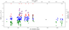 |
Fig. 1 Time series of Lindicator/Lbol- For the CARMENES LHα/Lbol we mark low activity states as green and blue dots, high activity states as red dots, flares as magenta dots, and spectra with an asymmetric Hα shape as cyan dots (see Sect. 6.1 for a detailed discussion). The cyan and magenta dots are labelled with the flare number also used in Fig. 9. Flare no. 14 is not shown here since the spectrum gets into absorption, and therefore no LHα/Lbol can be calculated with the χ method used here since it is only defined for emission lines. The ESPRESSO Hα measurements are marked as black triangles. The LX/Lbol measurement of the Chandra observation is marked as a black star; that of the XMM-Newton observation is marked as a black diamond. The time spans of the TESS observations are marked as small black dots connected by a black line. Since TESS is not photometrically calibrated, the position on the y-axis is arbitrary (we note here that for a blackbody of the temperature of Teegarden’s star about 20% of the radiation is in the TESS band). The red triangles mark the positions of the clusters of the higher activity states. |
2.3.2 ESPRESSO
We also used 11 spectra taken with the Echelle Spectrograph for Rocky Exoplanets and Stable Spectroscopic Observations (ESPRESSO) between 2019-09-21 and 2019-09-27, which we retrieved, reduced and flux-calibrated from the ESO archive4. The resolution of the spectra is 140 000, and they cover the range 3800-7900 Å; this means that ESPRESSO does cover the Ca II H & K lines, which are not covered by CARMENES, but are important for activity studies of solar-like stars (Baliunas et al. 1995; Suárez Mascareño et al. 2018; Perdelwitz et al. 2024).
2.3.3 Pseudo equivalent width measurements
To assess the activity state of Teegarden’s star in each spectrum, we employed pseudo-equivalent width (pEW) measurements, since late M dwarfs do not show an identifiable continuum because of the abundance of molecular absorption lines. For the used central wavelength, full width of the line integration window, the location of the two reference bands and a detailed description of pEW measurements of chromospheric lines, we refer to Fuhrmeister et al. (2023a,b).
3 Overview
The observations of Teegarden’s star were not part of a dedicated multi-wavelength campaign; nevertheless some of the data were taken (quasi-) simultaneously. To provide a better overview of the data, we show all used observations in Fig. 1. Hα pEWs are converted to LHα/Lbol-values by using the X-factor following the calculation by Reiners & Basri (2008). Our LHα/Lbol -values agree with calculations by Zechmeister et al. (2019). The LX/Lbol-values are calculated in Sect. 5.
Regarding the simultaneity of the data, we note that the XMM-Newton observation took place during the long observation gap of CARMENES, when also the TESS observations of sector 43 were obtained. The TESS sector as well as the XMM-Newton observation contains two significant flares (see Sects. 4.1 and 5.5 for a detailed discussion). The TESS observations of sectors 70 and 71 cover eight CARMENES spectra. These TESS observations show no apparent flare activity. Also the CARMENES pEW(Hα) values suggest a relatively low activity state for all of these spectra (for an empirical definition of the low activity state of Teegarden’s star regarding the Hα line see Fig. 1 and Sect. 6.1). The TESS observation of sector 71 ended 5 days before the next CARMENES spectrum, which was then in high activity state. The two adjacent TESS light curves could in principle be searched for signatures of the rotation period, which is with 97.6 days longer than even two TESS sectors, but no indications of rotational modulation can be identified.
The short timescales of the variations are demonstrated by the Chandra observation, which occurred only 5.5 hours after a CARMENES observation in high activity state. Nevertheless, it appears to cover the quiescent state of Teegarden’s star since the X-ray flux from the quiescent phases of the XMM-Newton observation is very similar (see Sect. 5). We therefore argue that this CARMENES observation may have covered a small flare or the decay phase of a larger flare, which ended before the Chandra observation started.
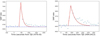 |
Fig. 2 TESS light curve of Flare I (left) and Flare II (right). The TESS data points are shown in blue, a simple analytic model is shown in red, and the assumed background is the blue dash-dotted line. |
4 Flaring activity observed by TESS
4.1 TESS flare light curves
We examined the light curves obtained in all three sectors, one from 2021, two from 2023. In the two sectors recorded in 2023 we could not find any obvious flares, while in 2021 two very obvious flares were recorded by TESS, which we call Flare I and Flare II for reference. We note that we are not saying that there are no more flares, but rather that any other flares are weaker and increasingly difficult to distinguish from the photometric noise.
The TESS short cadence data have a time resolution of 2 minutes, which is too long to adequately record flare light curves. An inspection of the TESS light curves (Fig. 2) shows that very few data points are actually ascribable to the flares. We therefore abstain from a detailed light curve modelling, rather we describe the TESS light curves with a simple linear rise followed by an exponential decay; already this model requires five parameters: the constant background level, the times of start and peak of the flare, the peak amplitude, and the decay time.
In Fig. 2 (left panel), we show the light curve of Flare I and a simple model curve. In Fig. 2, it can be seen that the flare rise is actually unresolved. Since the flare rise is usually much faster than the flare decay, the flare rise was probably shorter than two minutes and the flare amplitude larger than the largest recorded flux. A simple exponential decay does not adequately describe the full flare light curve, there appears to be some “fading out” on longer timescales.
Flare II looks similar to Flare I, and yet there are some differences: At least one data point is recorded during the flare rise, the overall amplitude is smaller than for Flare I, and yet the flare decay time is considerably longer. Again a simple exponential decay is an inadequate description of the flare light curve.
4.2 Energetics of TESS flares
In the following section we provide estimates of the energetics of Flare I and II shown in Fig. 2. These estimates are only rough estimates, since the temperature of the flaring material and its temporal evolution are unknown and cannot be deduced from the TESS data. For this reason it is also not worthwhile using actual flare model atmospheres, rather, following the approach applied by Shibayama et al. (2013), we take recourse to simple black-body models to describe the energetics of both the photospheric and flaring emission. One must bear in mind that the physical processes during a stellar flare are rather complicated and that stellar flares can have vastly different individual properties; for a detailed recent review of stellar flares and in particular flare modelling we refer to Kowalski (2024) and references therein.
To calibrate the recorded TESS light curves we use the stellar parameters listed in Table 1. Using the stellar distance and the effective temperature, and the TESS transmission curve we can compute the incident energy flux and thus derive the conversion factor to convert the observed TESS SAP rate into energy flux. Using this conversion factor also for the flare SAP rate and with some assumed effective temperature of the flaring material, we can compute the flare energy flux. Using the peak flare amplitude one can then determine the emitting area, and with the decay time, the total optical flare energy.
In Table 2, we list the parameters derived in this fashion. The physical flare parameters were computed by assuming temperatures of 15 000 K and 8000 K for the flaring plasma; since the flaring plasma is expected to change its temperature during the flare evolution, we may expect that the quantities listed in Table 2 provide reasonable estimates, which allow to put Flare I and II into a physical context. While there is admittedly quite some uncertainty w.r.t. the derived total flare energies, the numbers presented in Table 2 suggest that the flare energies involved are comparable to the flare energies of the largest solar flares observed (see Moore et al. (2014) for a discussion of total solar irradiance measurements of solar flares).
Seli et al. (2021) computed flare frequency distributions for very late-type M dwarfs observed with TESS. Inserting our flare energies in their Eq. (12) leads to an expectation of a flare like the ones we observed every 180 or 80 days for our largest and lowest flare energy, respectively. This is in rough agreement with our overall flare frequency of two flares in about 80 days which leads to 2.6±1.8 flares in 100 days. The occurrence of the two flares in just one sector, however, may hint at more active times of Teegarden’s star (cf. Sect. 6.1.3).
Flare parameters for Teegarden’s star from TES S light curves.
5 X-ray and UV observations with Chandra and XMM-Newton
5.1 Chandra X-ray source detection and flux determination
An analysis of the counting events received from the central source agrees with the position of Teegarden’s star to better than one arcsec, by taking the proper motion of the star into account. To determine the total number of counts recorded from Teegarden’s star, we determine the cumulative number of counts (CNC) in concentric rings centred on the observed source position. For the case of uniform background, CNC should increase quadrati-cally once no source photons contribute any longer. For the offset of the quadratic fit we find a value of 92.9 ± 1.7, which represents our best estimate for the recorded number of source counts from Teegarden’s star with a Poisson uncertainty of 9.8, which then translates into a (dead-time corrected) count rate of (1.96 ± 0.21) 10−3 cts/s.
To convert the observed count rate into an energy flux, we need to multiply with the energy-to-count conversion factor (ECF), which, however, depends on the assumed spectral parameters. The HRC data provide only very little energy resolution, hence no formal spectral fits are possible. Using PIMMS at NASA’s HEASARC (Mukai 1993), we can compute ECFs to convert the observed count rates To remedy this situation, we use temperature estimates from XMM-Newton. For “cool” temperatures in the range log T between 6.2 and 6.5 and abundances between solar and 0.4 sub-solar, these ECFs change very little (less than 1%), while larger changes occur for lower or higher temperatures. Using then an ECF of 1.09 × 10⁻¹¹ erg ct−1 cm−2, leads to an X-ray flux of 2.14 × 10⁻¹⁴ erg s−1 cm−2. With this flux one then computes - using the information in Table 1 -an X-ray luminosity LX of 3.7 × 1025 ergs−1 and a logarithmic LX/Lbol-ratio of −4.9.
5.2 Chandra X-ray variability
We next considered the temporal behaviour of the X-ray emission from Teegarden’s star as recorded by Chandra. To this end we constructed binned light curves using different choices of temporal binning, where the two highest bins occur adjacent to another right at the beginning of the observations (see Fig. 3). Performing a χ2 test we find variability at the significance level of ≈98%, somewhat depending on the precise choice of bins. A Kolmogorov-type analysis of the photon arrival times shows variability only at a slightly lower confidence level (90%). Thus we conclude that the X-ray emission of Teegarden’s star during the Chandra observations shows no larger flares, although some low-level variability is possibly present in the form of weaker flares.
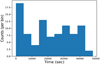 |
Fig. 3 Binned Chandra light curve of Teegarden’s star with time bins of ≈2500 s. |
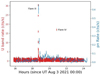 |
Fig. 4 XMM-Newton light curve for Teegarden’s star obtained with the OM in the U band (red data points, time resolution 10 s) and the EPIC pn detector (blue data points, time resolution 300 s). Flare III occurs at ~18.6 h and Flare IV occurs at ~20.9 h. |
5.3 XMM-Newton observations: Overview
To provide an overview over the whole XMM-Newton data set for Teegarden’s star, we plot in Fig. 4 both the XMM-Newton EPIC pn and OM light curves. Due to the rather different signal strengths different bin sizes were used, namely 10 s for the U band data and 300 seconds for the X-ray data. Both light curves show a rather low emission level for Teegarden’s star. However, in contrast to Chandra, the XMM-Newton X-ray data do show a rather major flare (Flare III), followed by some period of enhanced activity; the OM on board XMM-Newton even shows another flare (Flare IV), which we discuss in Sect. 5.5 in more detail; the lowest count rates, which we refer to as quiescence, were encountered at the beginning and end of the observation.
5.4 XMM-Newton observations: Quiescent emission
For Teegarden’s star the 4XMM DR13 catalogue lists a total EPIC mean count rate of 4.16 ± 0.14 10−2 cts/s and 714.6 source counts recorded in the pn detector; as obvious from Fig. 4, the star was in different states during the XMM-Newton observations. For low-flux sources it is difficult to define a true “quiescent” level. Assuming ad hoc that “quiescence” applies to the first 6800 seconds and last 8000 seconds (as in Fig. 4), we find no statistical differences in the recorded count rates in these two intervals. We further estimate that 22% of the number of total counts were recorded during this “quiescent” state and thus obtain a quiescent count rate of 2.4 × 10⁻² cts/s. Using again PIMMS at NASA’s HEASARC (Mukai 1993), we can compute energy flux conversion factors (ECF); for “cool” temperatures in the range log T between 6.2 and 6.5 and abundances between solar and 0.4 sub-solar, these ECFs change by about 10%. Using a flux conversion factor of 8.57 × 10⁻¹³ erg cm−2 s−1 (as appropriate for log T = 6.2), we derive a quiescent X-ray flux ƒX of 2.06 × 10⁻¹⁴ erg cm−2 s−1 and a quiescent X-ray luminosity LX of LX = 3.6 × 1025 ergs−1. We note that these fluxes and luminosities are very close to the respective values derived from the Chandra data.
Carrying out a similar exercise for the OM U band data, results in a mean U band rate of 0.45 ± 0.02 cts/s. To convert the observed U band rates by the XMM-Newton OM into fluxes, we use the calibration as presented in ESA’s XMM-Newton Calibration documentation5. Specifically, a conversion factor of 1.98 × 10⁻¹⁶ erg cm−2 ct−1 Å−1 has been derived to convert from observed rates to flux densities. This is again dominated by systematic errors, which we estimate to be of the order of 10%. With a U band width of 660 Å we can then convert the count rate to U band flux ƒU and find ƒU = 5.9 × 10⁻¹⁴ erg cm−2 s−1 and thus a total U band luminosity LU of 1.0 × 1026 erg s−1.
The level of X-ray emission in quiescence as measured by Chandra and XMM-Newton of about LX = 4 × 1025 erg s−1 puts Teegarden’s star among the weakest known stellar X-ray sources. However, if the relative X-ray luminosity is considered (i.e. the ratio of LX to Lbol), Teegarden’s value of lo𝑔(LX/Lbol) = −4.9 is much higher than the corresponding solar value, and yet computing the mean X-ray surface flux FX by dividing X-ray luminosity LX and stellar surface area  (cf. Table 1), one arrives at values in the vicinity of the minimal surface flux FX,min found by Schmitt (1997, Fig. 8) for cool main sequence stars; thus it appears that the minimal flux “law” is obeyed down to the lowest mass stars.
Wright et al. (2011) studied the X-ray emission of cool stars as a function of Rossby number (i.e. the ratio of the rotation period to convective turnover time). Inspecting their Fig. 2 and given the activity levels as measured for Teegarden’s star, one expects a Rossby number near unity, implying that the expected rotation period should be equal to the convective turnover time. Wright et al. (2011) also present an empirical determination of the convective turnover time; evaluation of their Eq. (11) yields a turnover time of ≈130 days given the mass of Teegarden’s star (cf. Table 1), which is indeed near the observed rotation period of 97.6 days (Shan et al. 2024).
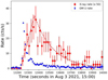 |
Fig. 5 Close-up view of XMM-Newton data for Flare III: OM U band rate (10 s bins, blue data points), merged EPIC X-ray rate (20 s bins, red data points), and flare model curve (dashed line). |
5.5 XMM-Newton observations: Flaring behaviour
The XMM-Newton light curve displayed in Fig. 4 shows two episodes of flaring activity, which we examine in more detail in this section. To this end we employ the highest possible time resolutions in the data. For the OM this is 1 second, while the X-ray data are limited by individual photon noise; to obtain the highest signal-to-noise ratio (S/N), we merge the X-ray data obtained with the three EPIC instruments and consider the recorded photon event arrival times.
In Fig. 5, we show the XMM-Newton data recorded for Flare III near 13 250 seconds. The U band light curve shows a rapid rise from quiescence to peak within 10 seconds, followed by a decay over the next 30 seconds; prior to the main flare rise, there appears to be some “pre-cursor” activity lasting for a few seconds. After the initial rapid flare decay one observes enhanced U band activity, which continues for quite some time as apparent from Fig. 4.
An inspection of the X-ray photon arrival times shows that during the time of Flare III in the U band very few X-ray photons were recorded, while the bulk of the X-ray emission occurs after the main U band event.
Specifically, in the 7 minutes after the U band Flare III, 127 X-ray photons where recorded, two thirds in the pn-detector and one third in the two MOS detectors with an estimated background contribution of fewer than 10 photons. Figure 5 shows that the counting statistics for the X-ray data is limited. However, from the data we estimate a lag between the maxima of U band and X-ray emission of about 100 seconds, the same timescale for the X-ray rise, and a decay time of around 175 seconds. We again note that both the U-band and X-ray emission appear to be enhanced for a while and do not readily return to pre-flare levels. The lag between U band peak and X-ray peak for Flare III is indicative of the Neupert effect and will be discussed in more detail in Sect. 5.7.
In Fig. 6, we show the XMM-Newton data recorded for Flare IV; we note that in contrast to Fig. 5, here the OM U band data are shown with a time resolution of 1 s. Figure 6 shows that the U band flare lasts only about 10 seconds, followed by some enhanced activity albeit at rather low levels. Somewhat surprisingly, no significant X-ray signal appears to be attributable to this UV event. In Fig. 6, we plot the arrival times of the recorded X-ray events around the UV event as red points. During the short U band flare no X-ray events were registered, a first X-ray event was recorded about 25 seconds after the flare peak, and another “group” of five photons about 100 seconds later. It is of course possible to interpret this “group” as an X-ray response to the U band flare, on the other hand, judging from the observed X-ray “background” rate prior and after the flare, one expects to obtain 2.8 counts in a 125 second interval; thus the observed 6 photons may equally well be interpreted simply as a statistical fluctuation. Therefore, to be on the safe side, we assume the total X-ray output of the flare to be <6 events.
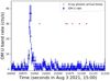 |
Fig. 6 Close-up view of XMM-Newton data for Flare IV. The OM U band rate (1 s bins) is shown as blue data points, while the arrival times of the recorded EPIC events are shown as red dots. |
5.6 XMM-Newton observations: Flare energetics
In the following section we focus on the energetics of the observed flaring X-ray and U band emission. To convert the U band rates observed by the XMM-Newton OM into fluxes we use the same procedure as in Sect. 5.4, and we list our results in Table 3. Further, to compute bolometric luminosities, we assume a blackbody spectrum for the emitting plasma with the same caveats applying; since we do not know the temperature we consider two temperature values, which hopefully bracket the true values.
As far as the X-ray energetics are concerned, we note that the derived peak luminosity depends somewhat on the chosen binning; however, Fig. 6 suggests that a value of 0.7 cts/s is a reasonable value. Since two thirds of this rate are due to counts in the pn detector, using an ECF of .11 × 10−12 erg cm−2 s−1 (as appropriate for log T = 6.8) leads to a peak X-ray luminosity of 9 × 1026 erg/s and a flare fluence of 1.6 ×1029 erg. At peak the X-ray output increased by a factor of more than 20, while the U band output increased by more than a factor of 100.
An inspection of the parameters listed in Table 3 shows that the energy emitted in the U band alone exceeds the energy emitted at X-ray wavelengths substantially. This discrepancy becomes even larger when the total energy is considered since the U band captures only some part of the emitted bolometric luminosity. The resulting values for the total emitted energies exceed the corresponding X-ray energies by more than an order of magnitude. While the derived values do by necessity carry large uncertainties, the conclusion appears inevitable that for the observed flares the photospheric energy output is larger by some order of magnitude than the coronal output. Such findings are not unusual; for example, Hawley et al. (1995) arrive at similar conclusions for a giant flare observed on AD Leo and Kuznetsov & Kolotkov (2021) find for eight out of nine flares with simultaneous X-ray and optical coverage that the optical flare output exceeds the corresponding X-ray output. The observed ratios between optical and X-ray output can vary substantially, and it is important to keep in mind that the flare site position on the stellar surface is normally unknown, and yet the observed optical emission from flares near the limb can be greatly suppressed (in contrast to X-ray emission).
Flare parameters for Teegarden’s star from XMM-Newton flares.
5.7 XMM-Newton observations: Neupert effect
5.7.1 The Neupert effect in stars
The Neupert effect, first described by Neupert (1968), constitutes, according to Kowalski (2024) (in chapter 7.7) ‘the backbone of the solar-stellar flare connection’. The Neupert effect describes an empirically found relationship between the hard and soft X-ray emission from solar flares. One often (albeit not always) observes that the observed hard X-ray emission shows the same temporal behaviour as the rate of change of the observed soft X-ray emission. Such hard X-ray emission is produced by bremsstrahlung from non-thermal electrons, which travel along the magnetic field lines and finally dissipate their energy in the solar chromosphere and photosphere, producing hot plasma. The hot plasma expands into the corona and radiates its energy as thermal X-ray radiation. In many cases, simultaneous hard and soft X-ray observations are not available, and then proxy indicators must be used; for example, Neupert (1968) actually used microwave emission as a proxy for non-thermal electrons and their (expected) hard X-ray emission.
In the stellar context, observations of the Neupert effect are relatively rare, and hard X-ray observations (in the sense of solar X-rays) of stellar flares do not exist. In many cases simultaneous observations with the necessary time resolution are not available. Guedel et al. (1996) present simultaneous X-ray observations (using ROSAT and ASCA) and radio observations (using the VLA at 6 cm and 3.6 cm) of the nearby flare star UV Cet and report a few cases of radio bursts followed by soft X-ray flares and argue that their observations do show a Neupert-like behaviour. Fuhrmeister et al. (2011) report simultaneous X-ray observations (using XMM-Newton) and VLT UVES observations of the nearby flare star Proxima Centauri and demonstrate a very good agreement between the time derivative of the X-ray light curve and the optical light curve. Tristan et al. (2023) report multi-wavelength observations of the flare star AU Mic, using a variety of different instruments including XMM-Newton and Swift in the X-ray range, the VLA at radio wavelengths and various ground-based observing facilities. In their data, Tristan et al. (2023) find 21 flares with overlapping data coverage, 16 of which are argued to show the Neupert effect.
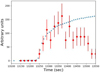 |
Fig. 7 Integrated XMM-Newton OM U band data (blue dots) in comparison to X-ray count rate (red data points with error bars) for Flare III. |
5.7.2 Neupert effect in Teegarden’s star
In the case of the XMM-Newton data of Teegarden’s star, we use the U band emission as proxy indicator for hard X-rays. Qiu (2021) show that UV emission is a good proxy indicator for heating and demonstrate that the observed X-ray emission can be well modelled in its rise; we note, however, that soft X-ray emission in a solar context differ from our soft X-ray data. In Fig. 7 we compare the time-integrated U band rate (blue dots) vs. the recorded (and arbitrarily scaled) X-ray flux (red data points with error bars) as a function of time for Flare III; we note that the low S/N of our data does not allow us to compute numerical derivatives, we rather use integrals of the observed UV emission. As is evident from Fig. 7, the agreement between these curves is very good, suggesting that indeed the Neupert effect is at work. On the other hand, only six data points describe the rise of the X-ray emission from the pre-flare level to the peak, thus the agreement might also be fortuitous to some extent.
6 Chromospheric activity as observed by CARMENES and ESPRESSO
6.1 Hα as main chromospheric indicator
6.1.1 General behaviour and flaring activity
Due to its location in the red wavelength region, where M dwarfs emit most, the Hα line at 6564.60 Å (vacuum wavelength, used for all CARMENES wavelengths) has been traditionally the most often used chromospheric line indicator. The LHα/Lbol of Teegarden’s star is shown in Fig. and exhibits strong variability.
We show a selection of spectra of Teegarden’s star around the Hα line in Fig. 8. Also directly in the spectra the huge range of variation can be seen. While in the quiescent state the line is more or less absent, during the most active states a strong emission line emerges. In the most quiescent states the line is hard to identify, and also comparison to a PHOENIX purely photospheric spectrum (Husser et al. 20 3) shows no larger discrepancies at the line position than at other wavelengths. Nevertheless, even the most inactive spectra show some variability at the Hα line indicating the presence of chromospheric emission. We show the comparison between observed and model Hα line in Fig. A.1.
When an emission line occurs, it is double horned, though not as pronounced as seen in more active M dwarfs such as G080-021 (M3.0 V, cf. Fig. 3 in Fuhrmeister et al. 2020), which exhibits an Hα emission line also during quiescent state. Nevertheless, among the very late-type stars, also vB 8 exhibits no or only a very shallow self-absorption feature (cf. Fig. 4 in Fuhrmeister et al. 2018). Although self-absorption should be symmetric from the theoretical point of view using one dimensional classical chromospheric models (Vernazza et al. 1981), Teegarden’s star shows a slightly higher red horn in some spectra. Many stars exhibit one horn preferentially higher than the other; for example, Proxima Centauri also shows a higher red horn for most of the time (Fuhrmeister et al. 2011). This asymmetry in the self-absorption is most probably caused by mass motions, which are not accounted for in classical chromospheric models, but can be included in hydrodynamic simulations of flaring plasma, which then also result in a higher red horn for various evolution stages of the flare (Allred et al. 2006).
For a better description of the variability, we identified from the spectral line shape four different activity states: (1) no line identifiable – very low activity state, (2) very small line observable – low activity state, (3) significant emission line – high activity state, (4) very pronounced emission line – flaring state. This empirical scheme by eye led to ‘fuzzy’ thresholds in pEW(Hα) and we therefore assigned each of these states an (arbitrarily chosen) threshold in pEW and mark them in Fig. 1. These thresholds are supported by a histogram of the LHα/Lbol values shown in Fig. A.2.
We believe it quite probable that all spectra of activity state (4) correspond to flares. Then Teegarden’s star as observed with CARMENES in Hα is 4.9% of the time in flaring state, and another 9.7% in high activity state (3). This flare duty cycle is only slightly higher than the 3% found in spectra of the Sloan digital sky survey (SDSS) for late-type M stars (Hilton et al. 2010). The much lower duty cycle of about 0.007% in the TESS band is caused by the red continuum wavelengths covered by the TESS band, which needs much higher flare energies involved compared to the Hα line to produce a notable flare reaction.
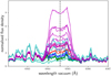 |
Fig. 8 Selected spectra of Teegarden’s star around the Hα line to demonstrate the line shape during quiescent phases and all flares. The spectra of activity level (1) are shown in green, of activity level (2) in blue, and of activity level (3) in red. The flare spectra are shown in magenta. There are a few spectra showing peculiar line shapes with broad additional line components either in absorption or emission (cyan lines). The dashed vertical line marks the central wavelength of Hα. The normalisation wavelength intervals are located well outside any broad wings at 6537.4–6547.9 and 6577.9–6586.4 Å. For the shown spectra the statistical errors are insignificant. |
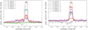 |
Fig. 9 Flare spectra and spectra with an unusual line shape with a mean quiescent spectrum subtracted. In the legend the spectra are ordered by occurrence time, and additionally the label from Fig. 1 is given. The spectra are split into two panels for clarity. |
6.1.2 Wing asymmetries
Next to the core line asymmetries, there are several wing asymmetries in the Hα line, as seen in Fig. 8 on the blue side of the pink and the brown spectra, which are above the other spectra around 6563 Å. Such wing asymmetries have been observed during flares (Fuhrmeister et al. 2018) and we mark these spectra with visually identified wing asymmetries in the pEW time series in Fig. 1.
To better demonstrate deviations from the usual line shape, we show all spectra which we have classified as flare spectra or to have an unusual line shape, with the mean quiescent spectrum subtracted, in Fig. 9. The flare spectra show a flat top and enhanced amplitudes, but no deviation from the quiescent spectrum outside the main line. The five spectra of unusual line shape, however, show broad wings. One spectrum with low amplitude (JD = 2 458 118.35) only has a symmetric slightly broader shape of unknown origin. Two spectra (JD = 2 458 060.48 and JD = 2460 164.59) have slight absorption lines in Hα and extended absorption wings at the blue side of the line (the latter being the only spectrum with positive pEW(Hα)). This may be caused by a prominence rotating at some height with the star. Another two spectra (JD = 2458 064.51 and JD = 2 458 064.65 in Fig. 9) show enhanced wings with more flux extending to lower than to higher wavelength. This suggests that the two spectra are taken during flare onsets, where blue asymmetries are expected due to chromospheric evaporations. The asymmetries are very broad and we refrain therefore from a Gaussian fit. They extend to about 6570 Å (~250 km s−1) on the red side and to 6558 Å (~−300 km s−1) on the blue side. While the escape velocity of Teegarden’s star is about 550 km s−1, the two spectra with blue asymmetries are taken by chance in the same night. Nevertheless, if this is a feature of a flare onset it cannot persist for such a long time (the spectra are taken about 3.4 hours apart). We think it is improbable that two flares happened consecutively each with only its onset covered by the two exposures. We therefore argue that we may see a coronal mass ejection (CME) under some inclination.
The two spectra belong to a concentration of flaring activity starting at about JD = 2 458 056 followed by another flare three days later (JD = 2 458 059). Again one day later one of the two spectra showing a broad absorption feature is taken (JD = 2 458 060; denoted by the green line in Fig. 9), followed by the two spectra exhibiting the strong blue emission wing (JDs = 2 458 064.51 and 2 458 064.65), which precede the strongest flare covered in our time series at JD = 2 458 065.46. That the possible CME follows one of the possible prominence features may hint at an eruption of the prominence.
6.1.3 Timing behaviour
Since we only have snapshot spectra, it is generally not possible to tell, which spectrum of higher activity state is caused by a flare, though decreasing pEW makes this more and more probable, but the threshold chosen here is arbitrary and some of the spectra with a high activity level (3) may be taken during decay phases of large flares, or be small flares themselves. Nevertheless, most of these high-activity pEWs seem to occur during active times longer than the typical duration of a few minutes to hours of a long-lasting Hα flare and group to some clusters, which may mark higher activity episodes of Teegarden’s star. Surprisingly these clusters are regularly spaced in time and are about 110 to 150 days apart of each other. We mark these clusters in Fig. 1 and the spacing is the following: 420, 110, 215, 148, 223 days (the numbers larger than 200 days are caused by observation gaps, but are about multiples of 110 days).
To further investigate this issue we have computed a periodogram of all the pEW(Hα) and only of the inactive phases (activity level (1) and (2)). We show the periodograms in Fig. 10. While all the data lead only to insignificant peaks with false alarm probability (FAP) lower than about 10% for all peaks, these are predominantly located at the same position as the peaks for the low activity data, which have a much better FAP. Only two peaks seem to stem from the higher activity data since they are absent in the low activity data. These peaks correspond to 112 and 161 days, where 161 days is a one-year alias of 112 days. This strongly supports the regularly cluster spacing of the high- activity data. If this is true, then a stable active region may be the origin of these flares. This would also hint at a higher latitude of this active region if the longer period is caused by solar-like differential rotation (with slower rotation towards the poles) in Teegarden’s star.
Further peaks appearing in the periodogram are found at 96 and 100 days, which are aliases of each other regarding the longest period of 2670 days. The peak at 78.8 days corresponds roughly to a one-year alias of 96 days, while the peak at 81.8 days corresponds to a one-year alias of 112 days. The peak at 1200 days is about half of the longest period peak. Therefore, the 2670-day period remains as the possible activity cycle (see below), as do the 112-day period of the clusters of higher activity and the 96-day period as rotation period (as is it very close to the 97.56-day period found by Shan et al. 2024). Instead, the 68.4-day period is still unexplained.
Next to the possible periodicity of the occurrence of the high-activity clusters, there may also be a periodicity present in the low activity pEWs of Hα and Ca II IRT of the observing season starting at JD = 2 457 949. We show a zoom-in on these data and the periodogram in Figs. A.4 and A.5. The period we find in these data has a broad peak at a frequency of about 0.0088 day−1 (i.e. at a period of 114 days). For all other observing seasons the number of observations is too low to do a timing analysis, therefore it may be a quasi-periodic episode, but the clustering of the higher activity states seems to persist on even longer timescales. Both timescales are only slightly higher than the literature rotation period of 97.56 days (Shan et al. 2024). This seems to indicate, that also during the lowest activity states an activity pattern rotating with the star may be seen, which is veiled for higher activity states (e.g. by dynamically changing Hα plages).
Although this remains speculative, there seems to be a really long variation pattern in the pEW(Hα) data: an upper envelope of the data seems first to drop and then to rise again (we show a zoom-in on that data in Fig. A.3), but even without the long data gap more data would be needed here for confirmation and a period determination. Now we can only crudely estimate a period of about 2500 days (~6.8 years), which could be caused by an activity cycle. Already Dreizler et al. (2024) drew a similar conclusion based on mostly the same CARMENES data, but from radial velocity measurements and activity line indices such as differential line width. In the framework of planet detection they found in their Gaussian process analysis a long period of at least the length of the data set and exhibiting a phase shift between radial velocity data and other activity indices, which has been found also for activity cycles on the Sun (Collier Cameron et al. 2019).
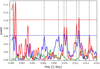 |
Fig. 10 Periodogram of all pEW(Hα) (blue line) and only activity level (1) and (2) (red line). A periodogram for the shuffled data is shown in green. The dashed blue line corresponds to a FAP level of 10% for the power shown in blue, while the dashed red line corresponds to a FAP level of 0.5% for the power shown in red. The dashed vertical lines mark the peaks corresponding to periods of 2670, 1200, 161, 112, 100, 96.4, 81.8, 78.8, and 68.4 days (from left to right). |
6.2 Other chromospheric line indicators
Next to the Hα line we analyse several other atomic lines, which have been used as chromospheric indicators (Gomes da Silva et al. 2012; Mittag et al. 2018; Schöfer et al. 2019; Fuhrmeister et al. 2020, 2023b; Lafarga et al. 2023). Depending on the spectrograph used, these are the Ca II IRT lines (at 8500.35, 8544.44, and 8664.52 Å), the Paschen series including Paβ, and the He I IR line (~10 830 Å), which are exclusively covered by CARMENES, while the Ca II H& K lines and the Balmer series lines Hβ, Hγ, Hδ, and Hє are only observed by ESPRESSO. The He I D3 line, the Na I D doublet, and the K I doublet at 7700 Å, are observed by both spectrographs.
Generally these lines fall into two types, first, purely chromospheric lines, which are not present in the photosphere, and second, lines, which also have a photospheric absorption line counterpart, which is filled in or shows emission cores. Due to the late M dwarf type, these photospheric absorption lines are quite shallow and very broad for Teegarden’s star. Since not many observations of all these chromospheric activity lines for such late and inactive M dwarfs like Teegarden’s star exist, we shortly comment on all of them in the following.
The Ca II H & K lines are seen as pronounced emission lines in the ESPRESSO spectra, but the photospheric absorption is not observed, since we do not detect continuum at these very blue wavelengths, as it is increasingly fainter for M dwarfs of later spectral type. Comparison to a PHOENIX spectrum shows that the continuum is not much lower than our detection limit with the exact numbers depending on the wavelength chosen for normalisation. We show the Ca II K line in Fig. 11.
The Balmer series members are all detected except Hє, with increasing amplitude to redder wavelength. None of these higher Balmer lines show a double peak structure like Hα. Since Teegarden’s star was in the most quiescent state during this time with little to nearly no Hα emission, the detection even of Hδ is a little bit surprising. We show as an example the Hβ line in Fig. 11.
The He I D3 line occurs as chromospheric emission line during three of the flares on Teegarden’s star and is absent in all other spectra. We show this behaviour in Fig. A.6. The neighbouring Na I D doublet shows only weak and broad photospheric absorption and also develops emission cores at line centre during the flares and enhanced activity periods, which we show in Fig. 12.
The same is true for the K I doublet, which exhibits very broad absorption features contaminated by noise and artefacts from telluric correction. Nevertheless, one can identify some emission cores in the centre of the photospheric absorption during some of the flares.
Regarding the Ca II IRT lines, the photospheric absorption is not really identifiable for the Ca II IRTa line, whose pEW nevertheless shows some variability. For the Ca II IRTb line a narrow and weak absorption line can be seen, which fills in for the flares. The Ca II IRTc absorption is blended with an Fe I line at 8664.28 Å and also develops a fill in for the flaring spectra. We show as an example the middle Ca II IRT line in Fig. A.7.
A weak absorption feature is found at the position of the Paβ line, which may at least partly be caused by a blend with a presumably molecular feature (Fuhrmeister et al. 2023b). No line is found at the position of the He I IR triplet. Since the He I D3 line is observed as emission line during the largest flares, we would expect some variability for these events also in the He I IR triplet. The reason that the flares are not seen in the IR line, may be the higher continuum level there than around the He I D3 line.
The pEWs of all of these lines, which are seen also during quiescence, correlate with pEW(Hα). The highest correlation is found for the Ca I IRTb line, with a Pearson’s correlation coefficient r of 0.81, while Ca I IRTa has 0.63, the blue Na I D line has 0.47, and the red K I line has 0.47; all with Pearson’s p < 10−18. We show as an example of these correlations the one between pEW(Hα) and pEW(Ca IRTb) in Fig. 13. The much weaker correlation of the Na I D and the K I line may be at least partly caused by the higher noise level, uncorrected airglow (both especially affect Na I D) and artefacts from the telluric correction.
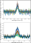 |
Fig. 11 All spectra of the Ca II K line (top) and of the Hβ line (bottom) taken with ESPRESSO. The black line denotes the mean spectrum. The Ca II K line has no continuum detected. |
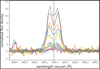 |
Fig. 12 Selected spectra of Teegarden’s star of the blue Na I D line to demonstrate the range of variation in this line. We show a few spectra of activity state (1) and all flares except two, which have a low signal- to-noise ratio in the continuum at these wavelength. |
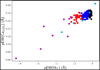 |
Fig. 13 Correlation of the pEW of the Ca I IRT middle line to Hα. The colours indicate the activity levels as in Fig. 1. The typical statistical errors are of the order of 1% and lower for both pEWs. |
7 Impact of the activity on the habitability of the innermost planets
The stellar X-ray and ultraviolet emission is a crucial factor thought to affect planetary habitability (Lammer et al. 2009). While the planets Teegarden’s star b and c may be suitable to harbour liquid surface water under a wide range of assumptions about the atmosphere (Wandel & Tal-Or 2019), it is doubtful whether this is sufficient to support the development of life. The effects of stellar high-energy irradiation on atmospheric erosion (e.g. Sanz-Forcada et al. 2011) and the atmospheric and surface chemistry on the planets (Ranjan et al. 2017; Spinelli et al. 2023) must be considered as well.
Adopting an X-ray luminosity of 4.2 × 1025 erg s−1 for Teegarden’s star (Table 1), we calculate X-ray fluxes at the orbital distances of the planets (Table 4). Assuming a typical value of 1027 erg s−1 for the X-ray luminosity of the Sun (e.g. Peres et al. 2000), we compare these to the current irradiating X-ray flux of the Earth ƒ⊕. While Teegarden’s star does not appear to be overly active by X-ray standards, the planets b, c, and d all receive higher X-ray fluxes than the Earth. In an Earthlike atmosphere, the incoming X-ray flux is absorbed high up in the atmosphere so that ground-level fluxes are negligible. The peak X-ray luminosity of the flare observed by XMM-Newton, exceeds the adopted quiescent luminosity by about a factor of three (Table 3), entailing correspondingly elevated irradiating fluxes. Whether the current irradiation levels and their variability prevent the evolution of life or are even required to foster chemical processes (Spinelli et al. 2023) remains unclear at this point.
X-ray fluxes at planetary orbit distance and comparison to Earth utilising recent X-ray fluxes at Earth ƒ⊕ (above the atmosphere).
8 Comparison to other late M dwarfs
Teegarden’s star is a rather inactive star for its spectral type, with a quiescent log LHα/Lbol ~ 5.4, compared to the typical range of log LHα/Lbol = −4.8 to −4.3 for M6–M7 stars as shown in Fig. 2 by Liebert et al. (2003). This better compares to the mean log LHα/Lbol = −4.79 including also flaring activity of Teegar- den’s star, and even that would place the star at the lower end of the typical quiescent activity range. This is in line to what one expects for such a slow rotator.
There are very few comparable flare measurements for late- type M dwarfs. For example, Fuhrmeister & Schmitt (2004) found for the M9 dwarf DENIS 104814.7−395606.1 during a flare a log LHα/Lbol = −4.00, which nicely fits the strength of the flares observed for Teegarden’s star (see Fig. 1). Also a flare on Proxima Centauri, which was studied by Fuhrmeister et al. (2011), led to log LHα/Lbol = −4.0. This study also encompassed X-ray observations covering the same flare, which allowed to measure log LX/Lbol = −4.1 and −2.9 during quiescent and flaring state, while for our larger X-ray flare we measure LX/Lbol = −4.38 , compared to a value of ~−5.0 in quiescence. This seems to indicate a different activity pattern for both stars, since the values inferred for Hα are comparable, while Proxima Centauri displays much higher X-ray radiation during the quiescent and flaring states.
For other late-type M dwarfs also more spectacular flares have been found. For example, Liebert et al. (1999) found for the M9.5 dwarf 2MASSW J0149090+295613 a quiescent log LHα/Lbol = −4.63, but during a spectacular flare log LHα/Lbol = −2.59. Since this flare also exhibited various emission lines in the red part of the spectrum its strength exceeded those of the flares observed on Teegarden’s star. Another large flare with asymmetries in the He I infrared triplet line and possibly in the Pa 6 line was studied by Kanodia et al. (2022) for vB 10 (M8). Although the Hα line was not covered, its strength could be estimated from the Ca IRT and Pa 7, which results in log LHα/Lbol estimates ranging from −2.8 to −3.2 for the flare. While the log LHα/Lbol of the quiescent state of these stars is comparable to Teegarden’s star, we could not identify such a mega-flare in our data and it stays elusive, if Teegarden’s star as relatively inactive star is capable of such strong flares.
Teegarden’s star is also interesting as a rare example of a very low-mass and slowly rotating star. It may serve as a testbed for estimating magnetic fluxes from rotation periods as was studied for M dwarfs by Reiners et al. (2022). For the rotation period of Teegarden’s star of 96 days, one arrives at a magnetic flux estimate of 1.7 × 1024Mx, using the equation from Table 2 of Reiners et al. (2022), and one can estimate LX and LHα from their Fig. 9 leading to LX = 6.3 × 1026 ergs−1 and LHα = 2.1 × 1026erg s−1. This is in contrast to our measured LX = 4.2 × 1025 erg s−1 (see Table 1) and LHα = 1.1 × 1025 erg s−1 (from log LHα/Lbol = −5.4 as our lowest quiescent estimate, see Fig. 1). Both measured values are about one order of magnitude lower than the expected values. Even, if we use our mean log LHα/Lbol = −4.79 ± 0.33 including flaring activity, there still remains a factor of five discrepancy. This should indicate, that the estimation of the magnetic flux from rotation period scales differently for these low-mass slow rotators (i.e. it also depends on mass).
9 Summary and conclusions
We studied the magnetically induced activity of Teegarden’s star by using 298 CARMENES spectra and 11 ESPRESSO spectra taken between 2016 and 2024, covering together all the usually used chromospheric activity indicator lines in the optical range. Moreover, we used three sectors of TESS observations for a search for large flares also affecting the red wavelengths covered by TESS (while smaller flares typically affect only bluer continuum wavelengths). Finally, we analysed one XMM-Newton and one Chandra observation to assess the X-ray properties of Teegarden’s star.
Of the optical chromospheric lines, only the He I IR triplet is not observed even during flares, which is probably caused by its location at rather red wavelengths, where any chromospheric emission must outshine the strongest part of the photospheric continuum, while the He I D3 line is observed in the spectra of the largest flares. The ESPRESSO spectra allow us to detect Ca II H & K and higher Balmer line emission up to Hδ, present also during quiescence. Many other chromospherically influenced lines are present in all observations and exhibit acceptable to good correlation with Hα, on which we therefore concentrated.
Our timing analysis of Hα exhibited a complex periodic behaviour, showing hints of an activity cycle of the length of the CARMENES observations, which was also found in the RV data (Dreizler et al. 2024). We also identify a peak in the periodogram at about the rotation period in the pEW(Hα) data and found indications of a periodic repetition of higher activity episodes at a slightly longer period of 112 days. In the lowest activity state of one observing season we also found a periodic behaviour of the same length, hinting at some rotating structure, which is veiled for higher activity states by Hα plage variations.
Thus, all data taken together paint the picture of a generally inactive star, which is nevertheless capable of producing substantial flaring. In pEW(Hα) we observe the star to be 4.9% of the time in a flaring state, which is slightly higher than what Hilton et al. (2010) observed for late M dwarfs in the SDSS. Moreover, in the Hα line shape and its asymmetries we find indications for a prominence erupting and maybe even causing a CME. In the X-ray range we also find large flares and we observe the Neupert effect in one flare, suggesting the production of non-thermal hard X-ray emission. Finally, the flare energetics derived from the X-ray and TESS data place these flares among large solar flares.
Acknowledgements
We acknowledge the help of J-U. Ness with the XMM- Newton OM data. We thank J. Sanz-Forcada for some discussions. This publication was based on observations collected under the CARMENES Legacy+ project. CARMENES is an instrument at the Centro Astronómico Hispano en Andalucía (CAHA) at Calar Alto (Almería, Spain), operated jointly by the Junta de Andalucía and the Instituto de Astrofísica de Andalucía (CSIC). The authors wish to express their sincere thanks to all members of the Calar Alto staff for their expert support of the instrument and telescope operation. CARMENES was funded by the Max-Planck-Gesellschaft (MPG), the Consejo Superior de Investigaciones Científicas (CSIC), the Ministerio de Economía y Competi- tividad (MINECO) and the European Regional Development Fund (ERDF) through projects FICTS-2011-02, ICTS-2017-07-CAHA-4, and CAHA16-CE-3978, and the members of the CARMENES Consortium (Max-Planck-Institut für Astronomie, Instituto de Astrofísica de Andalucía, Landessternwarte Königstuhl, Institut de Ciències de l’Espai, Institut für Astrophysik Göttingen, Universidad Complutense de Madrid, Thüringer Landessternwarte Tautenburg, Instituto de Astrofísica de Canarias, Hamburger Sternwarte, Centro de Astrobiología and Centro Astronómico Hispano-Alemán), with additional contributions by the MINECO, the Deutsche Forschungsgemeinschaft through the Major Research Instrumentation Programme and Research Unit FOR2544 “Blue Planets around Red Stars”, the Klaus Tschira Stiftung, the states of Baden-Württemberg and Niedersachsen, and by the Junta de Andalucía. We acknowledge financial support from the Agencia Estatal de Investigación (AEI/10.13039/501100011033) of the Ministerio de Ciencia e Innovación and the ERDF “A way of making Europe” through projects PID2021-125627OB-C31, PID2019-109522GB- C5[1:4], and the Centre of Excellence “Severo Ochoa” and “María de Maeztu” awards to the Instituto de Astrofísica de Canarias (CEX2019-000920-S), Instituto de Astrofísica de Andalucía (SEV-2017-0709) and Institut de Ciències de l’Espai (CEX2020-001058-M). This work was also funded by the Generali- tat de Catalunya/CERCA programme and the Agencia Estatal de Investigación del Ministerio de Ciencia e Innovación (AEI-MCINN) under grant PID2019- 109522GB-C53 and by the Deutsche Forschungsgemeinschaft under grant DFG SCHN 1382/4-1 This work made use of PyAstronomy (Czesla et al. 2019), which can be downloaded at https://github.com/sczesla/PyAstronomy.
Appendix A Chromospheric activity
We show in this section additional CARMENES data demonstrating the different chromospheric activity levels and involved timescales of Teegarden’s star.
Regarding the lowest activity state of Teegarden’s star, we compare a median spectrum of all spectra in activity level (1) with a model photospheric spectrum from the PHOENIX (Hauschildt et al. 1999) model spectrum library (Husser et al. 2013). We overplot here a model spectrum with Teff = 3000 K and log 𝑔 = 5.0 and solar chemical composition and show the comparison between model and observed spectrum in Fig. A.1. Although there are differences in the details, the overall spectral appearence is resembled quite well by the model, given that molecular data is notoriously badly known. Also at the location of the Hα line there are no larger deviations from the photospheric model seen.
In Fig. A.2 we show a histogram of the LHα/Lbol values of Teegarden’s star. At about LHα/Lbol=−4.9 there are lower numbers of spectra detected (which can be seen as gap most clearly in the observing season of 2016 in Fig. 1), which co-incises with our first threshold between activity level (1) and (2).
To make some of the features in Fig. 1 clearer, we show in Fig. A.3 a zoomed-in image of the low activity pEW(Hα)s to make the long-term variability of the upper envelope (but also of the lower envelope of the higher activity data marked in blue dots; however, this is not as clearly seen) visible more easily. In Fig. A.4 we zoom-in even further on the lowest activity pEW(Hα) data in one observing season, to show the periodic behaviour seen there. In Fig. A.5 we show the corresponding periodogram.
As further examples of chromospherically active lines we show in Fig. A.6 the He I D3 line and in Fig. A.7 the middle line of the Ca II IRT.
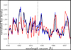 |
Fig. A.1 Comparison of the mean quiescent observed spectrum of Teegarden’s star (black line) to a PHOENIX photospheric model spectrum (red line) with Teff = 3000 K and log 𝑔 = 5.0 around Hα. Additionally we show two arbitrarily chosen spectra of low activity state (blue lines) demonstrating variability at the line position. While the dashed vertical line marks the position of the Hα line, the dashed horizontal line marks the normalisation level. |
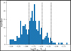 |
Fig. A.2 Histogram of the LHα/Lbol values. The thresholds between the (empirically defined) different activity states of Teegarden’s star are shown as dashed vertical lines. |
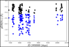 |
Fig. A.3 Time series of pEW(Hα) as in Fig. 1. We mark low activity states as black and blue dots, higher activity states as red dots, and spectra with an uncommon Hα shape with cyan dots. The upper envelope of the black dots show first an increase, then a decrease and again high pEW(Hα) values for the last data points. |
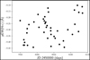 |
Fig. A.4 Time series of the most inactive pEW(Hα) of one observing season. |
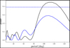 |
Fig. A.5 Periodogram of the pEW(Hα) (black line) and pEW(Ca IRT 8544Å) (blue line). The dashed horizontal line marks the FAP = 0.01 level. |
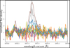 |
Fig. A.6 Selected CARMENES spectra of Teegarden’s star of the He I D3 line. The shown spectra are the same as in Fig. 12. |
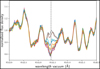 |
Fig. A.7 Selected CARMENES spectra of Teegarden’s star of the middle Ca II IRT line. The line shows a fill in during flares. The shown spectra are the same as in Fig. 12. |
References
- Allred, J. C., Hawley, S. L., Abbett, W. P., & Carlsson, M. 2006, ApJ, 644, 484 [NASA ADS] [CrossRef] [Google Scholar]
- Alonso-Floriano, F. J., Morales, J. C., Caballero, J. A., et al. 2015, A&A, 577, A128 [NASA ADS] [CrossRef] [EDP Sciences] [Google Scholar]
- Baliunas, S. L., Donahue, R. A., Soon, W. H., et al. 1995, ApJ, 438, 269 [Google Scholar]
- Brun, A. S., & Browning, M. K. 2017, Liv. Rev. Sol. Phys., 14, 4 [Google Scholar]
- Caballero, J. A., Guàrdia, J., López del Fresno, M., et al. 2016, Proc. SPIE, 9910, 99100E [Google Scholar]
- Collier Cameron, A., Mortier, A., Phillips, D., et al. 2019, MNRAS, 487, 1082 [Google Scholar]
- Czesla, S., Schröter, S., Schneider, C. P., et al. 2019, PyA: Python astronomy-related packages, Astrophysics Source Code Library [record ascl:1906.010] [Google Scholar]
- Dreizler, S., Luque, R., Ribas, I., et al. 2024, A&A, 684, A117 [NASA ADS] [CrossRef] [EDP Sciences] [Google Scholar]
- Dumusque, X., Udry, S., Lovis, C., Santos, N. C., & Monteiro, M. J. P. F. G. 2011, A&A, 525, A140 [NASA ADS] [CrossRef] [EDP Sciences] [Google Scholar]
- Fuhrmeister, B., & Schmitt, J. H. M. M. 2004, A&A, 420, 1079 [NASA ADS] [CrossRef] [EDP Sciences] [Google Scholar]
- Fuhrmeister, B., Lalitha, S., Poppenhaeger, K., et al. 2011, A&A, 534, A133 [NASA ADS] [CrossRef] [EDP Sciences] [Google Scholar]
- Fuhrmeister, B., Czesla, S., Schmitt, J. H. M. M., et al. 2018, A&A, 615, A14 [NASA ADS] [CrossRef] [EDP Sciences] [Google Scholar]
- Fuhrmeister, B., Czesla, S., Hildebrandt, L., et al. 2020, A&A, 640, A52 [NASA ADS] [CrossRef] [EDP Sciences] [Google Scholar]
- Fuhrmeister, B., Czesla, S., Perdelwitz, V., et al. 2023a, A&A, 670, A71 [NASA ADS] [CrossRef] [EDP Sciences] [Google Scholar]
- Fuhrmeister, B., Czesla, S., Schmitt, J. H. M. M., et al. 2023b, A&A, 678, A1 [NASA ADS] [CrossRef] [EDP Sciences] [Google Scholar]
- Gaia Collaboration (Brown, A. G. A., et al.) 2018, A&A, 616, A1 [NASA ADS] [CrossRef] [EDP Sciences] [Google Scholar]
- Giampapa, M. S., & Liebert, J. 1986, in Cool Stars, Stellar Systems and the Sun, 24, eds. M. Zeilik & D. M. Gibson, 62 [NASA ADS] [CrossRef] [Google Scholar]
- Gillon, M., Triaud, A. H. M. J., Demory, B.-O., et al. 2017, Nature, 542, 456 [NASA ADS] [CrossRef] [Google Scholar]
- Gomes da Silva, J., Santos, N. C., Bonfils, X., et al. 2012, A&A, 541, A9 [NASA ADS] [CrossRef] [EDP Sciences] [Google Scholar]
- Guedel, M., Benz, A. O., Schmitt, J. H. M. M., & Skinner, S. L. 1996, ApJ, 471, 1002 [NASA ADS] [CrossRef] [Google Scholar]
- Hauschildt, P. H., Allard, F., & Baron, E. 1999, ApJ, 512, 377 [Google Scholar]
- Hawley, S. L., Fisher, G. H., Simon, T., et al. 1995, ApJ, 453, 464 [NASA ADS] [CrossRef] [Google Scholar]
- Hilton, E. J., West, A. A., Hawley, S. L., & Kowalski, A. F. 2010, AJ, 140, 1402 [Google Scholar]
- Husser, T.-O., Wende-von Berg, S., Dreizler, S., et al. 2013, A&A, 553, A6 [NASA ADS] [CrossRef] [EDP Sciences] [Google Scholar]
- Jenkins, J. M., Twicken, J. D., McCauliff, S., et al. 2016, SPIE Conf. Ser., 9913, 99133E [Google Scholar]
- Kanodia, S., Ramsey, L. W., Maney, M., et al. 2022, ApJ, 925, 155 [NASA ADS] [CrossRef] [Google Scholar]
- Kowalski, A. F. 2024, Liv. Rev. Sol. Phys., 21, 1 [NASA ADS] [CrossRef] [Google Scholar]
- Kuznetsov, A. A., & Kolotkov, D. Y. 2021, ApJ, 912, 81 [NASA ADS] [CrossRef] [Google Scholar]
- Lafarga, M., Ribas, I., Zechmeister, M., et al. 2023, A&A, 674, A61 [NASA ADS] [CrossRef] [EDP Sciences] [Google Scholar]
- Lammer, H., Bredehöft, J. H., Coustenis, A., et al. 2009, A&A Rev., 17, 181 [NASA ADS] [CrossRef] [Google Scholar]
- Liebert, J., Kirkpatrick, J. D., Reid, I. N., & Fisher, M. D. 1999, ApJ, 519, 345 [NASA ADS] [CrossRef] [Google Scholar]
- Liebert, J., Kirkpatrick, J. D., Cruz, K. L., et al. 2003, AJ, 125, 343 [NASA ADS] [CrossRef] [Google Scholar]
- Marfil, E., Tabernero, H. M., Montes, D., et al. 2021, A&A, 656, A162 [NASA ADS] [CrossRef] [EDP Sciences] [Google Scholar]
- Mittag, M., Schmitt, J. H. M. M., & Schröder, K. P. 2018, A&A, 618, A48 [NASA ADS] [CrossRef] [EDP Sciences] [Google Scholar]
- Mohanty, S., & Basri, G. 2003, ApJ, 583, 451 [NASA ADS] [CrossRef] [Google Scholar]
- Moore, C. S., Chamberlin, P. C., & Hock, R. 2014, ApJ, 787, 32 [NASA ADS] [CrossRef] [Google Scholar]
- Mukai, K. 1993, Legacy, 3, 21 [Google Scholar]
- Murray, S. S., Chappell, J. H., Kenter, A. T., et al. 1997, SPIE Conf. Ser., 3114, 11 [NASA ADS] [Google Scholar]
- Nagel, E., Czesla, S., Kaminski, A., et al. 2023, A&A, 680, A73 [NASA ADS] [CrossRef] [EDP Sciences] [Google Scholar]
- Neupert, W. M. 1968, ApJ, 153, L59 [NASA ADS] [CrossRef] [Google Scholar]
- Perdelwitz, V., Trifonov, T., Teklu, J. T., Sreenivas, K. R., & Tal-Or, L. 2024, A&A, 683, A125 [NASA ADS] [CrossRef] [EDP Sciences] [Google Scholar]
- Peres, G., Orlando, S., Reale, F., Rosner, R., & Hudson, H. 2000, ApJ, 528, 537 [NASA ADS] [CrossRef] [Google Scholar]
- Qiu, J. 2021, ApJ, 909, 99 [NASA ADS] [CrossRef] [Google Scholar]
- Quirrenbach, A., CARMENES Consortium, Amado, P. J., et al. 2020, SPIE Conf. Ser., 11447, 114473C [Google Scholar]
- Ranjan, S., Wordsworth, R., & Sasselov, D. D. 2017, ApJ, 843, 110 [Google Scholar]
- Reiners, A., & Basri, G. 2008, ApJ, 684, 1390 [Google Scholar]
- Reiners, A., Shulyak, D., Käpylä, P. J., et al. 2022, A&A, 662, A41 [NASA ADS] [CrossRef] [EDP Sciences] [Google Scholar]
- Ribas, I., Reiners, A., Zechmeister, M., et al. 2023, A&A, 670, A139 [NASA ADS] [CrossRef] [EDP Sciences] [Google Scholar]
- Ricker, G. R., Winn, J. N., Vanderspek, R., et al. 2015, J. Astron. Telesc. Instrum. Syst., 1, 014003 [Google Scholar]
- Sanz-Forcada, J., Micela, G., Ribas, I., et al. 2011, A&A, 532, A6 [NASA ADS] [CrossRef] [EDP Sciences] [Google Scholar]
- Schmitt, J. H. M. M. 1997, A&A, 318, 215 [NASA ADS] [Google Scholar]
- Schöfer, P., Jeffers, S. V., Reiners, A., et al. 2019, A&A, 623, A44 [Google Scholar]
- Seli, B., Vida, K., Moór, A., Pál, A., & Oláh, K. 2021, A&A, 650, A138 [NASA ADS] [CrossRef] [EDP Sciences] [Google Scholar]
- Shan, Y., Revilla, D., Skrzypinski, S. L., et al. 2024, A&A, 684, A9 [NASA ADS] [CrossRef] [EDP Sciences] [Google Scholar]
- Shibayama, T., Maehara, H., Notsu, S., et al. 2013, ApJS, 209, 5 [Google Scholar]
- Spinelli, R., Borsa, F., Ghirlanda, G., Ghisellini, G., & Haardt, F. 2023, MNRAS, 522, 1411 [NASA ADS] [CrossRef] [Google Scholar]
- Suárez Mascareño, A., Rebolo, R., González H ernández, J. I., et al. 2018, A&A, 612, A89 [NASA ADS] [CrossRef] [EDP Sciences] [Google Scholar]
- Teegarden, B. J., Pravdo, S. H., Hicks, M., et al. 2003, ApJ, 589, L51 [Google Scholar]
- Tristan, I. I., Notsu, Y., Kowalski, A. F., et al. 2023, ApJ, 951, 33 [NASA ADS] [CrossRef] [Google Scholar]
- Vernazza, J. E., Avrett, E. H., & Loeser, R. 1981, ApJS, 45, 635 [Google Scholar]
- Wandel, A., & Tal-Or, L. 2019, ApJ, 880, L21 [NASA ADS] [CrossRef] [Google Scholar]
- Weisskopf, M. C., O’Dell, S. L., & van Speybroeck, L. P. 1996, SPIE Conf. Ser., 2805, 2 [NASA ADS] [Google Scholar]
- Wright, N. J., Drake, J. J., Mamajek, E. E., & Henry, G. W. 2011, ApJ, 743, 48 [Google Scholar]
- Yadav, R. K., Christensen, U. R., Morin, J., et al. 2015, ApJ, 813, L31 [Google Scholar]
- Zechmeister, M., Anglada-Escudé, G., & Reiners, A. 2014, A&A, 561, A59 [NASA ADS] [CrossRef] [EDP Sciences] [Google Scholar]
- Zechmeister, M., Dreizler, S., Ribas, I., et al. 2019, A&A, 627, A49 [NASA ADS] [EDP Sciences] [Google Scholar]
The XMM-Newton SAS user guide can be found at https://xmm-tools.cosmos.esa.int/external/xmm_user_support/documentation/sas_usg/USG/
All Tables
X-ray fluxes at planetary orbit distance and comparison to Earth utilising recent X-ray fluxes at Earth ƒ⊕ (above the atmosphere).
All Figures
|
Fig. 1 Time series of Lindicator/Lbol- For the CARMENES LHα/Lbol we mark low activity states as green and blue dots, high activity states as red dots, flares as magenta dots, and spectra with an asymmetric Hα shape as cyan dots (see Sect. 6.1 for a detailed discussion). The cyan and magenta dots are labelled with the flare number also used in Fig. 9. Flare no. 14 is not shown here since the spectrum gets into absorption, and therefore no LHα/Lbol can be calculated with the χ method used here since it is only defined for emission lines. The ESPRESSO Hα measurements are marked as black triangles. The LX/Lbol measurement of the Chandra observation is marked as a black star; that of the XMM-Newton observation is marked as a black diamond. The time spans of the TESS observations are marked as small black dots connected by a black line. Since TESS is not photometrically calibrated, the position on the y-axis is arbitrary (we note here that for a blackbody of the temperature of Teegarden’s star about 20% of the radiation is in the TESS band). The red triangles mark the positions of the clusters of the higher activity states. |
| In the text | |
|
Fig. 2 TESS light curve of Flare I (left) and Flare II (right). The TESS data points are shown in blue, a simple analytic model is shown in red, and the assumed background is the blue dash-dotted line. |
| In the text | |
|
Fig. 3 Binned Chandra light curve of Teegarden’s star with time bins of ≈2500 s. |
| In the text | |
|
Fig. 4 XMM-Newton light curve for Teegarden’s star obtained with the OM in the U band (red data points, time resolution 10 s) and the EPIC pn detector (blue data points, time resolution 300 s). Flare III occurs at ~18.6 h and Flare IV occurs at ~20.9 h. |
| In the text | |
|
Fig. 5 Close-up view of XMM-Newton data for Flare III: OM U band rate (10 s bins, blue data points), merged EPIC X-ray rate (20 s bins, red data points), and flare model curve (dashed line). |
| In the text | |
|
Fig. 6 Close-up view of XMM-Newton data for Flare IV. The OM U band rate (1 s bins) is shown as blue data points, while the arrival times of the recorded EPIC events are shown as red dots. |
| In the text | |
|
Fig. 7 Integrated XMM-Newton OM U band data (blue dots) in comparison to X-ray count rate (red data points with error bars) for Flare III. |
| In the text | |
|
Fig. 8 Selected spectra of Teegarden’s star around the Hα line to demonstrate the line shape during quiescent phases and all flares. The spectra of activity level (1) are shown in green, of activity level (2) in blue, and of activity level (3) in red. The flare spectra are shown in magenta. There are a few spectra showing peculiar line shapes with broad additional line components either in absorption or emission (cyan lines). The dashed vertical line marks the central wavelength of Hα. The normalisation wavelength intervals are located well outside any broad wings at 6537.4–6547.9 and 6577.9–6586.4 Å. For the shown spectra the statistical errors are insignificant. |
| In the text | |
|
Fig. 9 Flare spectra and spectra with an unusual line shape with a mean quiescent spectrum subtracted. In the legend the spectra are ordered by occurrence time, and additionally the label from Fig. 1 is given. The spectra are split into two panels for clarity. |
| In the text | |
|
Fig. 10 Periodogram of all pEW(Hα) (blue line) and only activity level (1) and (2) (red line). A periodogram for the shuffled data is shown in green. The dashed blue line corresponds to a FAP level of 10% for the power shown in blue, while the dashed red line corresponds to a FAP level of 0.5% for the power shown in red. The dashed vertical lines mark the peaks corresponding to periods of 2670, 1200, 161, 112, 100, 96.4, 81.8, 78.8, and 68.4 days (from left to right). |
| In the text | |
|
Fig. 11 All spectra of the Ca II K line (top) and of the Hβ line (bottom) taken with ESPRESSO. The black line denotes the mean spectrum. The Ca II K line has no continuum detected. |
| In the text | |
|
Fig. 12 Selected spectra of Teegarden’s star of the blue Na I D line to demonstrate the range of variation in this line. We show a few spectra of activity state (1) and all flares except two, which have a low signal- to-noise ratio in the continuum at these wavelength. |
| In the text | |
|
Fig. 13 Correlation of the pEW of the Ca I IRT middle line to Hα. The colours indicate the activity levels as in Fig. 1. The typical statistical errors are of the order of 1% and lower for both pEWs. |
| In the text | |
|
Fig. A.1 Comparison of the mean quiescent observed spectrum of Teegarden’s star (black line) to a PHOENIX photospheric model spectrum (red line) with Teff = 3000 K and log 𝑔 = 5.0 around Hα. Additionally we show two arbitrarily chosen spectra of low activity state (blue lines) demonstrating variability at the line position. While the dashed vertical line marks the position of the Hα line, the dashed horizontal line marks the normalisation level. |
| In the text | |
|
Fig. A.2 Histogram of the LHα/Lbol values. The thresholds between the (empirically defined) different activity states of Teegarden’s star are shown as dashed vertical lines. |
| In the text | |
|
Fig. A.3 Time series of pEW(Hα) as in Fig. 1. We mark low activity states as black and blue dots, higher activity states as red dots, and spectra with an uncommon Hα shape with cyan dots. The upper envelope of the black dots show first an increase, then a decrease and again high pEW(Hα) values for the last data points. |
| In the text | |
|
Fig. A.4 Time series of the most inactive pEW(Hα) of one observing season. |
| In the text | |
|
Fig. A.5 Periodogram of the pEW(Hα) (black line) and pEW(Ca IRT 8544Å) (blue line). The dashed horizontal line marks the FAP = 0.01 level. |
| In the text | |
|
Fig. A.6 Selected CARMENES spectra of Teegarden’s star of the He I D3 line. The shown spectra are the same as in Fig. 12. |
| In the text | |
|
Fig. A.7 Selected CARMENES spectra of Teegarden’s star of the middle Ca II IRT line. The line shows a fill in during flares. The shown spectra are the same as in Fig. 12. |
| In the text | |
Current usage metrics show cumulative count of Article Views (full-text article views including HTML views, PDF and ePub downloads, according to the available data) and Abstracts Views on Vision4Press platform.
Data correspond to usage on the plateform after 2015. The current usage metrics is available 48-96 hours after online publication and is updated daily on week days.
Initial download of the metrics may take a while.