| Issue |
A&A
Volume 690, October 2024
|
|
|---|---|---|
| Article Number | A383 | |
| Number of page(s) | 11 | |
| Section | Planets and planetary systems | |
| DOI | https://doi.org/10.1051/0004-6361/202451582 | |
| Published online | 23 October 2024 | |
XUV irradiation of young planetary atmospheres. Results from a joint XMM-Newton and HST observation of HIP67522
1
INAF-Osservatorio Astronomico di Palermo,
Piazza del Parlamento 1,
90134
Palermo,
Italy
2
Department of Physics and Chemistry, University of Palermo,
Piazza del Parlamento 1,
90134
Palermo,
Italy
★ Corresponding author; antonio.maggio@inaf.it
Received:
19
July
2024
Accepted:
9
September
2024
Context. The evaporation and the chemistry of the atmospheres of warm and hot planets are strongly determined by the high-energy irradiation they receive from their parent stars. This is more crucial among young extra-solar systems because of the high activity of stars at early ages. In particular, the extreme-ultraviolet (EUV) part of the stellar spectrum drives significant processes of photochemical interaction, but it is not directly measurable because of strong interstellar absorption and a lack of sufficiently sensitive instrumentation. An alternative approach is to derive synthetic spectra from the analysis of far-ultraviolet (FUV) and X-ray emission lines, which allow us to estimate the missed flux in the EUV band.
Aims. We performed joint and simultaneous spectroscopy of HIP 67522 with XMM-Newton and the Hubble Space Telescope in order to reconstruct the full high-energy spectrum of this 17 Myr-old solar-type (G0) star, which is the youngest transiting multiplanet system known to date.
Methods. We performed a time-resolved spectral analysis of the observations, including quiescent emission and flaring variability. We then derived the emission measure distribution (EMD) versus temperature of the chromospheric and coronal plasma from the high-resolution spectra obtained in X-rays with RGS and in FUV with COS.
Results. We derived broad-band X-ray and EUV luminosities from the synthetic spectrum based on the EMD, which allowed us to test alternative EUV versus X-ray scaling laws available in the literature. We also employed the total X–EUV flux received by the inner planet of the system to estimate its instantaneous atmospheric mass-loss rate.
Conclusions. We confirm that HIP 67522 is a very active star with a hot corona, reaching plasma temperatures above 20 MK even in quiescent state. Its EUV/X-ray flux ratio falls in between the predictions of the two scaling laws we tested, indicating an important spread in the stellar properties, which requires further investigation.
Key words: planets and satellites: gaseous planets / planet-star interactions / stars: activity / stars: coronae / stars: late-type / planetary systems
© The Authors 2024
 Open Access article, published by EDP Sciences, under the terms of the Creative Commons Attribution License (https://creativecommons.org/licenses/by/4.0), which permits unrestricted use, distribution, and reproduction in any medium, provided the original work is properly cited.
This article is published in open access under the Subscribe to Open model. Subscribe to A&A to support open access publication.
1 Introduction
Since the discovery of the first extra-solar planet around a main sequence star in 1995 by Mayor & Queloz (1995), the search for exoplanets has received an outstanding push forward in several directions. Huge efforts are devoted today to characterizing planetary atmospheres, and to understanding the formation and evolution processes leading to the observed variety of planetary masses and sizes. Nowadays, there are more than 5000 confirmed planets and thousands of Kepler and TESS (Transiting Exoplanet Survey Satellite) candidate planets (Batalha et al. 2013, https://exoplanet.eu, https://doi.org/10.26134/ExoFOP5). However, the available target sample is dominated by relatively old stars because of difficulties in planet discovery around active (young) stars with current instrumentation and detection techniques. The frequency of planets depends on their masses, sizes, and host star properties, and is a key parameter for testing planet formation and evolution models. On the other hand, evolutionary paths are the result of the complex interplay between physical and dynamical processes operating on different timescales, including the stellar radiation fields. In particular, intense high-energy irradiation from the host stars, especially at young ages, can be responsible for evaporation of exoplanet atmospheres; this process is one of the ingredients that shapes the planet mass–radius relationship but is still poorly understood (Lopez & Fortney 2013; Owen & Wu 2013; Fulton et al. 2017; Owen & Wu 2017; Fulton & Petigura 2018; Owen & Lai 2018; Modirrousta-Galian et al. 2020). For these reasons, there are several ongoing observation programs at optical and IR wavelengths targeting relatively young stars. In particular, TESS is providing unprecedented opportunities for exoplanet searches around stars in young moving groups and stellar associations. Planets in these stellar environments are particularly important because the ages of the systems can be determined more accurately than for field stars. However, these photometric surveys can only provide measurements of planetary radii, while determination of masses still requires spectroscopic follow-up with ground-based facilities. For this reason, the italian GAPS collaboration is currently leading a long-term program with the HARPS-N (optical) and GIANO-B (NIR) spectrographs at the Telescopio Nazionale Galileo (TNG) in La Palma (Carleo et al. 2020; Damasso et al. 2020), and we have conducted similar Guest Observer programs with the HARPS spectrograph at the ESO-3.6 m in La Silla. The aim of these programs is to constrain planetary masses and orbital parameters of selected TESS and Kepler young planets using the radial velocities technique. With our programs, we contributed to validating the presence of the first young TESS candidate, namely DS Tuc Ab (40 Myr, Benatti et al. 2019), and the planetary system around the 50 Myr K star TOI-942 (Carleo et al. 2021). For these and other young systems (V 1298 Tau, 10–30 Myr, Maggio et al. 2022; TOI-837, 35 Myr, Damasso et al. 2024), we also reconstructed the photoevaporation histories.
The structure of planetary atmospheres sensitively depends on the spectral energy distribution of the stellar radiation (Lammer et al. 2003). While extreme-ultraviolet (EUV) photons are absorbed in the upper atmosphere, soft X-rays can heat and ionize lower layers due to the cascade of secondary electrons (Cecchi-Pestellini et al. 2006). Reliable characterization of planetary evolution requires knowledge of the whole stellar high- energy emission and its variability (Sanz-Forcada et al. 2011; Locci et al. 2019). Planets in close orbits around young stars (t < 100 Myr) are especially susceptible to irradiation effects because of the higher activity levels relative to the Sun and the stronger magnetic fields.
Higher magnetic activity is generally accompanied by more frequent and energetic flares (Davenport 2016), and higher rates of coronal mass ejection (CME) are expected as well (Khodachenko et al. 2007). In turn, charged particle flows linked to stellar winds and CMEs determine the size and time-dependent compression of planetary magnetospheres, and eventually may lead to stripping (erosion) of close-in planets (Lammer et al. 2007), as well as deposition of gravity waves (Cohen et al. 2014). A detailed characterization of the high- energy emission (1–1700 Å, hereafter XUV emission) of young stars hosting exoplanets is highly desirable with XMM-Newton or Chandra and the Hubble Space Telescope (HST) at present, in the era of the James Webb Space Telescope (JWST) and in view of the forthcoming Ariel mission in 2029.
HIP 67522 (HD 120411) is a member of the Sco-Cen young association (5–20 Myr), located at a distance of 124.7 ± 0.3 pc. It hosts a Jupiter-size transiting planet discovered in the TESS survey and validated by Rizzuto et al. (2020), with an orbital period of ~6.96 d, and a planetary radius of 10.07 ± 0.47 R⊕, but just a loose constraint of its mass in the range 0.18–4.6 MJ. Moreover, this planet is likely undergoing Kelvin-Helmholtz contraction and photoevaporation (Heitzmann et al. 2021), meaning that its mass could be lower than those of mature planets with similar radii (Lopez & Fortney 2013). By measuring the Rossiter- McLaughlin effect during transits, Heitzmann et al. (2021) also determined the orbital inclination of HIP 67522b, and discovered that it is well-aligned in spite of its young age, thus ruling out a migration history driven by high eccentricity. The planet is also a compelling target for atmospheric characterization, and the system was indeed observed in 2023 with JWST (PI: A.W. Mann, GO 2498).
The system also contains a second smaller planet (Rp = 8.2 ± 0.5 R⊕) with a period of 14.96 d, which was recently confirmed by Barber et al. (2024) to be in near 2:1 mean motion resonance with HIP 67522 b. This discovery makes HIP 67522 the youngest system known to date to have two transiting planets.
In the present paper, we describe our analysis of simultaneous observations of HIP 67522 with XMM-Newton and HST in order to acquire high-resolution spectra from FUV to soft X-rays, and to determine the emission measure distribution of the optically thin plasma from the outer chromosphere to the corona, and the full XUV irradiation of the planets. This, in turn, is crucial input for modeling their atmospheric evaporation and photo-chemistry.
The structure of the paper is as follows: Sect. 2 describes the observations and the data analysis, Sect. 3 presents the results of the analysis, and Sect. 4 contains a discussion and our final conclusions.
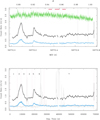 |
Fig. 1 X-ray and NUV light curves of HIP 67522. Top: light curves of EPIC (black pn, dark and light blue MOS 1,2) and OM (green) instruments. The EPIC light curves were binned at 600 s per bin, while the OM light curve was binned at 90 s. The OM rate is divided by 5 for making easier the comparison. The horizontal bars on the top indicate the time of the HST/COS exposures. The top axis reports the orbital phases of the planet. The vertical dotted lines mark ingress and midtransit times of the planet. Bottom: EPIC light curves and time intervals defining flares 1 and 2 rise+peak and decay (2, 3, 5, 6) and quiescent levels (1, 4, 7). The gray light curve refers to background single events with energies between 10 keV and 12 keV, in the full field of view of the pn detector. |
2 Observations
HIP 67522 was observed in X-rays with XMM-Newton for about 70 ks (PI: A. Maggio, ObsId: 0902070101) on July 11, 2022. Together with the European Photon Imaging Camera (EPIC), we used the Optical Monitor (OM) with the filter UVM2, whose band-pass is 200–300 nm, in order to monitor the near-ultraviolet (NUV) emission of the star, and the Reflection Grating Spectrograph (RGS) for high-resolution spectroscopy in the band 5-35 Å.
Figure 1 shows the light curves of EPIC and OM instruments. Two flares are evident in the EPIC light curve, while the OM light curve shows an overall modulation on timescales of longer than the exposure time and comparable with the rotation period of the star itself (Prot = 1.418 ± 0.016 d, Rizzuto et al. 2020). We simultaneously observed the FUV emission of HIP 67522 with the HST Cosmic Origins Spectrograph (COS) during three consecutive orbits (program id: LESW01010) in order to obtain spectra with the G130M grism in the band 1170-1420 Å (central wavelength: 1291 Å). The coverage of HST orbits during the XMM-Newton exposures is shown in Fig. 1. Due to an issue with the acquisition of the target, only the second exposure was successful in providing a COS spectrum of the star.
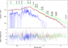 |
Fig. 2 EPIC and RGS global spectra, and best-fit 3T VAPEC model. Black and red data points for the MOS1 and MOS2, while the pn spectrum is in green, and the summed RGS1+RGS2 spectra in blue. The main complexes of H-like and He-like ions are indicated. |
2.1 Analysis of XMM-Newton data
The observation data files (ODFs) constituting the XMM-Newton observation were retrieved from the XMM-Newton archive and reduced with XMM-SAS version 20.0.0. For the MOS and pn observations, we obtained calibrated event lists in the band 0.3– 8.0 keV. The source events were extracted from a circular region with a radius of 60″ , while the background was extracted from a close region with similar size and devoid of other sources. From these files, we obtained source and background light curves (Fig. 1). Inspection of the light curve of events detected with energies E > 10 keV allowed us to identify and filter out few time intervals affected by high background, as prescribed in the XMM-SAS guide. Finally, we extracted the source spectra along with the relative response files, and applied a rebinning in order to get at least 30 counts per energy bin and a signal-to-noise ratio (S/N) of at least five for each spectral bin of EPIC spectra, and 10 counts per bin in the case of RGS (Fig. 2).
We reduced the data from the OM and from the RGS to obtain a light curve in the band 200–300 nm and a high- resolution spectrum in the ~5–35 Å wavelength interval. The first-order spectra of RGS1 and RGS2 were summed together in order to improve the counting statistics and cover the gap of the missing chips in each detector (Fig. 3).
We then performed a global spectral analysis of the EPIC and RGS spectra jointly (Fig. 2, Sect. 3.1) for the entire length of the observation. The spectra were analyzed with XSPEC version 12.12. We adopted an optically thin plasma emission model with three isothermal components (VAPEC), and including absorption by the interstellar medium (TBabs model, with ISM abundances by Wilms et al. 2000). The free parameters for the best-fit procedure were the interstellar H column density (NH), the temperatures (kT), the emission measure (EM) of each component, and the abundances of several elements scaled to the solar one (Ab(Z)/Ab(Z)⊙, shared by all components). The goodness of the fit was evaluated with chi-square statistics, and the uncertainties on the best-fit values were computed at the 90% statistical confidence level with the XSPEC error procedure.
As the X-ray emission was variable during the XMM-Newton exposure (Fig. 1), we also performed a time-resolved spectral analysis, dividing the observation into seven intervals (Sect. 3.2). For each interval, we accumulated the combined spectrum of PN, MOS1, and MOS2, and built the appropriate spectral response and effective area files with the SAS tasks rmfgen and arfgen. High photon rates can produce pile-up and distortion of the spectrum, especially in pn. In our case, we checked with the SAS epatplot task that the pile-up fraction is negligible1, even in the interval of highest rate during the first flare, and that further corrections are not necessary. The same conclusion applies to the global spectra introduced above.
Subsequently, the emission lines of the coronal ions in the combined RGS spectra of the global observation were measured with Pint Of Ale version 2.954 (PoA, Kashyap & Drake 1998, 2000), and employed for the reconstruction of the plasma emission measure distribution versus temperature, EMD(T) (Sect. 3.3), together with the chromospheric and transition region lines measured in the HST spectra. Table A.1 reports the measurements of the coronal line fluxes employed in the analysis.
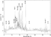 |
Fig. 3 RGS spectrum of the full exposure, with the identifications of the most prominent emission lines. |
2.2 Analysis of HST data
The COS spectra of the HST observations were retrieved from the HST archive, ready to be analyzed. These spectra were acquired with COS and the G130M filter calibrated in both fluxes and wavelengths with errors (Fig. 4). The FUV lines for which we measured the fluxes are listed in Table A.1. To this aim, we adopted a Moffat’s line profile function that can adequately describe both the core and the wings of the COS lines. Using both FUV fluxes from COS ion lines and X-ray fluxes measured in RGS spectra, we reconstructed the EMD(T) as described in Sect. 3.3.
3 Results
3.1 Global spectral analysis
HIP 67522 is an active star with a quite hot corona. The global pn and MOS spectra (Fig. 2) clearly show the line complexes due to H-like and He-like ions of S and Ca, and also the Fe XXV He-like line, indicating plasma components with temperatures above 10 MK. In effect, the best-fit model includes plasma in the range 5–25 MK, with the hottest component dominant in terms of volume emission measure (Table 1).
We left the chemical abundances of O, Ne, Mg, Si, S, Ca, and Fe free to vary (Table 2). The abundances of C and N were linked to that of oxygen, while Al, Ar, and Ni remained linked to iron. The pattern of element abundances versus first ionization potential (FIP; Fig. 5), suggests a FIP bias typical of young active stars (Maggio et al. 2007; Scelsi et al. 2007).
The best-fit model also provides a measure of NH = 2.3 × 1019 cm−2, with a 1σ upper limit of <7.9 × 1019 cm−2. This value agrees with the absorption expected if we assume a mean interstellar hydrogen density of 0.07–0.1 cm−3, typical of the solar neighborhoods. In addition, the value is in good agreement with the empirical relationship of Redfield & Linsky (2000), which yields NH ≃ 3.9 × 1019 cm−2. The E(B − V) < 0.05 color excess (Rizzuto et al. 2020) provides a looser constraint of NH < 2 × 1020 cm−2.
Best-fit parameters obtained with XSPEC of spectra during each time interval.
 |
Fig. 4 Spectra of HIP 67522 obtained with COS and grism G130M (central wavelength 1291 Å). Top: FUVB segment (~1140–1280 Å). Bottom: FUVA segment (~1290–1420 Å). The main lines are labeled. |
Element abundances derived from the analysis.
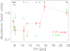 |
Fig. 5 Element abundances versus first ionization potential from the global fitting of the EPIC+RGS spectra with a 3T model, and from the emission measure analysis of the COS and RGS line fluxes. |
3.2 Time-resolved analysis and flares
The EPIC light curves show two flares with peaks occurring at approximately 9 and 18 ks after the start of the exposures. The first flare has a relatively symmetrical profile, with the rise and decay phases each having a duration of about 3 ks, while the second flare shows a more usual profile, with a rapid rise (t ~ 1 ks) followed by a slower decay of t ~ 5 ks.
While the flares are clearly visible in soft X-rays, only the first one is barely visible in the OM band pass (200–300 nm) at a planetary phase of ~0.902, while the second one is much less apparent as its peak occurred during a gap between two subsequent OM exposures. For the first flare, the delay between the peak in NUV and in X-rays is about 2.8 ± 0.3 ks, and is a signature of the Neupert effect (Neupert 1968; Hudson 1991). The plasma within a loop is first heated and the UV peak probes the rise in temperature; the gas then evaporates through the feet of the loop and fills it, with an increase in the plasma density and the X-ray emission mirroring the rise and peak of the emission measure within the loop (Namekata et al. 2017).
In order to perform time-resolved spectroscopy of the quiescent and flaring phases, we divided the light curve into seven intervals, as shown in Fig. 1 (lower panel). For each flare, we considered the rise up to the peak as a first interval where, presumably, we can measure the peak of the plasma temperature (intervals 2 and 5), and a second interval with the decay after the peak (intervals 3 and 6). The quiescent phases were those preceeding the two flares (intervals 1 and 4), and the final phase after the second flare (interval 7). The latter has the longest duration, and the spectrum of the combined pn and MOS instruments accumulated during this interval has 43 930 counts. We fit this spectrum with a model composed of three VAPEC components (see Table 1), fixing all the abundance ratios with respect to iron at the best-fit values found in the global fit, and leaving only the iron abundance free to vary. We obtained a cool component at around 6.5 MK, a mild component at around 11 MK, and a hot component at 23 MK.
Since the spectral shape is similar in intervals 1, 4, and 7, for the spectra 1 and 4 we used the same 3T VAPEC model derived from the best fit to the spectrum 7, with only the three emission measures left to vary. In this manner, we trace the slight differences (~20% in flux) between these quiescent intervals, while maintaining a minimal number of free parameters, suitable for the lower photon counting statistics in these brief pre-flare intervals.
For the flare segments, we separated the phases of rise + peak and the decay (intervals 2 and 3 for the first flare, and 5 and 6 for the second flare), and used the 3T model from the best fits in the pre-flare phases as a quiescent basal emission, to which we added a fourth APEC component to describe the flaring plasma. The maximum temperatures in the flares are about 110 MK ( keV) and 60MK (
 keV) during the first and second flare, respectively. The presence of very hot plasma is clearly seen as an enhancement of the highly ionized Fe XXV lines at 6.7 keV.
In the hypothesis of a quasi-static cooling of the loop after the flare, it is possible to apply simple diagnostics to infer the semi-length of the loop (Serio et al. 1991; Reale 2007, 2014). The relevant equations are:
 (1)
(1)
where L9 is the loop semi-length in units of 109 cm, ζ is the slope of the decay in the 1 /2 log(EM) − log(T) plane, τLC is the e-folding time of the light-curve decay, T7 is the maximum temperature of the flare in units of 107 K and calibrated from the observed maximum temperature Tobs inferred from the model best fit to the spectra:
 (2)
(2)
The correction to the formula of Serio et al. (1991) for a quasi-static decaying loop in case of residual heating during the decay is
 (3)
(3)
with parameters estimated from extensive simulations of observations with the EPIC instrumentation (see Reale 2007).
Using the decay e-folding times (1.5 and 2.2 ks for the first and second flare, respectively) and the maximum observed temperatures (see above), we inferred a semi-length of about 6– 7 × 1010 cm, similar for both flares. This value corresponds to about 60–70% of the stellar radius. Assuming an aspect ratio of 0.1 between the radius and length of the loop, we derived a volume of about 1.8–2.1 × 1031 cm3. From the volume and emission measure EM4 relative to segments 2 and 4, we inferred an electron density of 7–11 × 1010 cm−3 , which appears high when compared to the densities recorded during solar flares, but similar to the values of other flares in young stars (Getman & Feigelson 2021).
We estimated the energy released in each flare by summing the net luminosity of the flaring component (LX,flare), obtained by subtracting the luminosity in the preflare intervals, multiplied by the duration of each flaring interval (2–3 and 5–6). This resulted in values of ≃2.1 × 1034 erg and ≃7.6 × 1033 erg for the two respective flares. Similar energies have been detected in other young-planet-hosting stars, such as DS Tuc A (Pillitteri et al. 2022); these energies are more than one order of magnitude larger than typical flares occurring in the Sun. Flares releasing energies of E > 1034 ergs in X-rays are often referred to as “super flares” (see e.g., Getman & Feigelson 2021).
The minimum magnetic field required to constrain the plasma in the loop can be calculated as:

where kB is the Boltzmann’s constant, and ne,peak and Tpeak are the density and the temperature at the flare peak. We inferred minimum fields of Bmin ≥ 460 G and Bmin ≥ 270 G for the two respective flares.
3.3 Derivation of the emission measure distribution
The line fluxes from COS and RGS were analyzed with the PoA software in order to derive the emission measure distribution, EMD(T), as a function of plasma temperature. We adopted Chianti version 7.13 as the atomic database for line emissivities. For this analysis, we also employed the continuum flux measured in four wavelength regions devoid of lines, derived with XSPEC from the model best fitting the global EPIC+RGS spectrum. These additional measurements (Table A.1) allow us to constrain the absolute abundances of iron and the other elements.
The plasma EMD(T) versus temperature was obtained iteratively with the PoA Monte Carlo Markov Chain procedure by simultaneously varying the emission measure in each temperature bin and the abundances of each element so as to match the measured fluxes. To this aim, we considered a subset of measured line fluxes, as reported in Table A.1. In particular, we did not consider density-sensitive lines, lines with uncertain identification, and lines whose fluxes appear mutually incompatible in the hypothesis of collisionally excited plasma (Maggio et al. 2023).
Considering the temperature ranges covered by the emissivities of the selected lines, we derived the EMD over a temperature grid ranging from log T = 4.0 to log T = 7.45, with Δ log T = 0.15. The results are shown in Fig. 6 and listed in Table 3, together with a plot of the residuals between observed and predicted line fluxes (Table A.1).
In principle, the use of the average RGS X-ray spectrum acquired during both quiescent and flaring states, in conjunction with the COS FUV lines acquired only during the quiescent state, can introduce a bias in the hot part of the EMD. Here, we verified that this choice implies a negligible correction of the total flux in the X-ray band (Sect. 3.4). Moreover, frequent flares are typical of very young and active stars, and should therefore be taken into account, at least in a statistical sense, when evaluating the time-averaged stellar emission level. Hence, it is justified to consider the full exposure RGS spectrum, which helps to reduce the uncertainties on the measured X-ray line fluxes.
The element abundances of the model with the highest likelihood and their 1σ uncertainties are reported in Table 2 and shown in Fig. 5. These abundances were found to be compatible with the values from the global fitting of X-ray spectra for the elements N, Ne, Mg, and Fe, while the C, O, S, and Si abundances differ by factors of ~3. Part of the discrepancy can be due to the assumption that the mixing ratios of all the species remain constant in the full range of temperatures explored, while the abundances likely change somewhere between the chromosphere and the corona. Moreover, some differences may be due to the two different atomic databases employed for the analysis of the global spectra and of the emission lines.
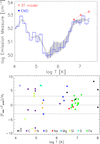 |
Fig. 6 Results of the joint analysis of XMM-Newton/RGS and HST/COS spectra. Top: Plasma EMD vs. temperature, compared with the 3-T model (red points) best fitting the global EPIC and RGS spectra. The shaded band represents a smoothed 1σ confidence region. Bottom: differences, in σ units, between measured line fluxes and predicted values vs. temperature at the peak emissivity. The black “H” symbols represent narrow-band measurements of the X-ray continuum. Empty symbols are lines not used for the EMD reconstruction. |
3.4 Scaling between X-ray and EUV fluxes
We computed synthetic XUV spectra from the EMD(T) presented above (Sect. 3.1), and then the X-ray luminosity in the 5–100 Å band, and the EUV luminosity in the 100–920 Å band. We obtained best values of LX = 3.43 × 1030 erg s−1 and LEUV = 2.80 × 1030 erg s−1. To evaluate the uncertainties on the luminosities, we determined the 2.5–97.5 percentile ranges of the luminosity distributions obtained from the Monte Carlo sampling of the EMD(T) and abundances parameter space. The ranges are thus 3.37 – 3.63 × 1030 erg s−1 on LX and 2.66 – 3.56 × 1030 erg s−1 on LEUV. The corresponding range of LEUV/LX ratios is 0.76–1.00.
As we employed the full-exposure RGS spectra, the EMD above ∼106 K also takes into account the presence of the flares that occurred during the observation. However, their effect on the broad-band X-ray luminosity remains negligible, because the RGS band is softer than the EPIC band and is less sensitive to very hot plasma. Indeed, the values of X-ray luminosity derived with EPIC spectra during the quiescent intervals 1, 4, and 7 is consistent with the range of X-ray luminosity derived from the synthetic spectrum based on the EMD.
Figure 7 shows our EUV and X-ray measurements for HIP 67522, together with a few other benchmark stars with exoplanets already considered in Maggio et al. (2023). The sample of G-K dwarfs employed by Johnstone et al. (2021, J21) to calibrate their X-ray to EUV scaling law is also shown. In the same plot, we repropose this scaling law and the alternative scaling law by Sanz-Forcada et al. (2022, SF22), with the respective 90% confidence regions. In the latter case, where the original relation is based on EUV vs. X-ray luminosities, we show two confidence regions in the FEUV/FX vs. FX plot, which were obtained assuming two different values for the stellar radius2. We stress that the empirical power laws are based on heterogeneous samples of about 20 single or binary stars, with spectral types from F to M, and observed in X-rays or UV wavelengths at different epochs.
Among the benchmark stars, selected to cover a wide range of activity levels, we included our Sun, with flux ranges derived from Johnstone et al. (2021) and based on observations with the TIMED/SEE mission. As intermediate-activity stars, we show the cases ofHD 189733 (Sanz-Forcada et al. 2011; Bourrier et al. 2020) and є Eri (Sanz-Forcada et al. 2011; Chadney et al. 2015; King et al. 2018). For the latter, we adopted the X-ray luminosity range derived by Coffaro et al. (2020), because the EUV measurement is not simultaneous. At the high-activity extreme, an interesting comparison case is provided by V 1298 Tau, a young planet-hosting star similar to HIP 67522, for which we derived an X-EUV spectrum following the same observation and analysis approach as in the present case (Maggio et al. 2023).
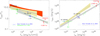 |
Fig. 7 X-ray vs. EUV scaling laws and benchmark stellar sample. (Left) Measurements of the EUV to X-ray ratio vs. X-ray flux at the stellar surface for HIP 67522, the Sun, and other G-K-type stars. The names indicate benchmark stars with exoplanets. Different X-ray (5–100 Å) to EUV (100–920 Å) scaling laws are shown for comparison: the gray band indicates the 90% confidence region relative to the J21 scaling law (green dashed line). The golden band is the 90% confidence region for the SF22 scaling law, assuming stars with radii equal to that of HIP 67522, while the orange band is for stars with 0.7 R⊙. The ranges for the Sun indicate its variability during an entire magnetic cycle. (Right) Analogous plot for the scaling laws of the EUV vs. X-ray luminosities. The gold dashed lines represent an extrapolation of the SF22 solution, while the gray-shaded area comprises stars with radii in the range 0.7–1.38 R⊙. |
Emission measure distribution.
3.5 Planetary irradiation spectrum
We employed our EMD(T) solution to synthesize the full XUV spectrum in the range 1–1700 Å (Fig. 8), and extended it to the visible wavelength range by adding the photospheric contribution predicted for a star with Teff = 5700 K, log g = 4.0, and solar metallicity (Rizzuto et al. 2020) based on the PHOENIX stellar library (Husser et al. 2013). We also overplot the flux measured with the XMM/OM in the UVM2 band (1830–2790 Å), computed on the Vega flux scale: taking a range of the OM count rate ~11–14 ct s−1 from Fig. 1, for HIP 67522 (mv = 13.03) we derived a source intensity of fMUV = 2.39–3.05 × 10⁻¹⁴erg s−1 cm−2 Å−1, which translates into a flux of FMUV = 2700–3500 erg s−1 cm−2 (2.7–3.5 W m−2) at the planet distance (a ~ 0.076 AU). We make the synthetic spectrum of HIP 67522 in FITS format available for download from the Zenodo archive3. The file contains the tables with the energy, wavelength, and flux at 1 AU along with the EMD(T) used to synthesize it and the element abundances Ab(Z)/Ab(Z)⊙.
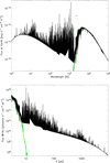 |
Fig. 8 Composite spectrum of HIP 67522 obtained by joining the Phoenix photospheric spectrum with the XUV spectrum synthesized from the reconstructed plasma emission measure distribution vs. temperature in the chromosphere, transition region, and corona. The upper panel shows the specific flux at Earth, while the bottom panel is the photon flux at a distance of 1 AU. The Phoenix spectrum resampled down to ~1700 Å with a wavelength resolution of 1 Å is shown in green; the XUV spectrum in the range 1–1700 Å is shown instead with a resolution of 0.01 Å. The green and blue segments in the upper panel, at ~200 nm, mark the Phoenix model flux and the observed flux integrated over the OM UVM2 band. |
3.6 Planetary photoevaporation
We employed the measured X-ray and EUV fluxes to compute the atmospheric mass-loss rate of the planet HIP 67522b using the analytical approximation based on the ATES hydrodynamic code (Caldiroli et al. 2021, 2022). In order to evaluate possible evaporation timescales, we also need an educated guess of the atmospheric mass fraction, which we derived from the planetary core–envelope models by Fortney et al. (2007) and Lopez & Fortney (2014). To this aim, we assumed an ice/rock composition of the core of 25%/75%. In practice, most of the uncertainty in modeling the planet structure rests in the planetary mass, which is poorly constrained (0.18–4.6 MJ, Rizzuto et al. 2020). Considering that the planetary radius is just 10% lower than the size of Jupiter, we explored four cases corresponding to two values of mass, Mp = 0.18 MJ or 1 MJ, and two possible values of atmospheric metallicity, yielding solar or enhanced opacities (see Lopez & Fortney 2014).
At the nominal radius of HIP 67522b, the system of equations that describe the planetary structure allows only one solution with a relatively large and massive core. Table 4 shows the values of the core mass, core radius, and atmospheric mass fraction at present age in the four cases. Assuming that the core mass and size remain constant in time, the envelope radius and atmospheric mass fraction evolve in response to gravitational contraction and to photoevaporation, the latter driven by the X-EUV irradiation.
At its present age, the X-EUV flux (5–920 Å) is found to be ~3.9 × 10⁵ erg s−1 cm−2 at the planet, which is relatively high, and implies a strong energy loss due to advective and radiative cooling if the gravitational potential is low enough (Caldiroli et al. 2022). This is our low-mass case for HIP 67522b, that is, in a low-gravity regime of the atmospheric hydrodynamic outflow, which occurs when the volume-averaged mean excess energy due to photo-heating exceeds the gravitational binding energy. As a consequence, the ATES model predicts a photoevaporation efficiency of η ~ 14% with respect to the energy-limited threshold (Erkaev et al. 2007). The efficiency is even lower in the high-mass case, that is, in a high-gravity regime: η ~ 0.2%. This is because advective cooling and Lyα energy losses dominate over adiabatic expansion and cooling. This difference leads to a mass-loss rate of ~10−2 M⊕/Myr in the low-mass case, or ~3 × 10⁻⁵ M⊕/Myr in the high-mass case (Table 4). Depending on the planetary mass and structure, the instantaneous e-folding evaporation timescale will be relatively short (300–600 Myr) in the low-mass case, or extremely long (>>10 Gyr) in the high-mass case.
The actual long-term evolution of the planetary mass and radius depends on the rate of decrease in the stellar activity and its X-EUV emission with age, and on the relative role of mass loss with respect to gravitational contraction during the evolution (see e.g., Mantovan et al. 2024; Damasso et al. 2024). Such a highly refined modeling is premature for HIP 67522b, given the poor knowledge of the actual planetary mass.
4 Discussion and conclusions
In this paper, we present the results from simultaneous observations of HIP 67522 with XMM-Newton and HST in X-ray and FUV bands. The quiescent X-ray luminosity of this target, Lx ~ 3 × 1030 erg s−1 , is very high and in line with that expected for a 1.2 M⊙ star at an age of 15–18 Myr (Johnstone et al. 2021). The high activity level is also mirrored by the hardness of the X-ray spectrum, which is due to the presence of plasma at temperatures exceeding 20 MK.
The star also exhibited two moderately bright flares separated by ~9 ks; these flares released energies of between 8 × 1033 and 2 × 1034 erg. In this respect, they appear similar in energy and timing to a couple of flares detected in DS Tuc A, which is 40 Myr old and of similar stellar mass (Pillitteri et al. 2022). We speculate that such twin flares in young coronae could be triggered in the same loop or in adjacent loops due to the packed structuring of the magnetic field. At the distance of the planet, the X-ray flux received during the two flares was ∽790 and ∽630 Wm−2.
From a different perspective, Ilin et al. (2024) recently presented a survey of optical flares in planet-hosting stars detected during the Kepler and TESS space missions. In particular, they searched for flaring events clustered in orbital phase, as a proxy of star–planet magnetic interactions. HIP 67522 was found to be the target most likely characterized by this kind of behavior based on the distribution of 12 flares observed in three sectors of the TESS sky coverage.
We derived the volume emission measure distribution of the plasma vs. temperature, which provides an overall description of the average thermal structure of the plasma from the upper chromosphere to the corona. In Fig. 9 we compare the EMD of HIP 67522 to those of a few other G-K stars with different activity levels and already considered in Maggio et al. (2023). In particular, we note the similarity between the EMDs of HIP 67522, V 1298 Tau, and DS Tuc in the corona (T > 106 K), along with an excess of emission measure for HIP 67522 in the chromosphere and transition region.
The EUV/X-ray flux ratio for HIP 67522, inferred from the synthetic spectrum based on the average EMD, places this young active star in between the two alternative scaling laws of Johnstone et al. (2021) and Sanz-Forcada et al. (2022). This FEUV/FX ratio is larger, at the 1σ level, than the value we derived for V 1298 Tau, which was also based on simultaneous X-ray and FUV observations analyzed with a methodology similar to the present case (Maggio et al. 2023). This result is explained by the different shapes of the EMDs, and it suggests that there is an intrinsic uncertainty, by at least a factor 2, on the EUV flux derived for other stars, when only X-ray measurements are available, depending on the assumed scaling law. An uncertainty of similar size can be systematic in origin, and due to different possible methodologies employed to reconstruct the EMD(T) and hence to estimate indirectly the EUV flux from available X-ray and FUV spectra (Maggio et al. 2023).
We employed the total X-EUV flux to study the photoevaporation of HIP 67522 b using the ATES code (Caldiroli et al. 2022). However, the large uncertainty in the planetary mass (0.18–4.6 MJ) yields a relatively loose range of possible massloss rates. For a mass of >1 MJ, we estimate a rate of log M < 9.7 (g/s), which implies an evaporation e-folding timescale of >>10 Gyr. For the lower limit on mass of 0.2 MJ, we determine an instantaneous mass-loss rate of log Ṁ ∽ 12.4 (g/s), which amounts to ≃4 × 10⁻⁵ MJ/Myr. Considering an atmospheric mass fraction in the range of 18–36%, the low-mass case yields an e-folding evaporation timescale within the age of stars in the Hyades open cluster. However, the actual planetary evolution is highly nonlinear, because the planetary high-energy irradiation should decrease by about a factor 5 within 600 Myr and by a factor 10 within 2 Gyr due to the natural decay of stellar activity (Johnstone et al. 2021). On the other hand, for a planet in the low- gravity regime (Sect. 3.6), a lower X-EUV flux leads to higher photoevaporation efficiency. We defer more detailed simulations of the photoevaporation history of HIP 67522 – as already performed for V 1298 Tau (Maggio et al. 2022) – to a time when the planet mass has been assessed with future radial velocity followup campaigns. As a final result, we derived a synthetic XUV spectrum for HIP 67522, which will be useful for future studies of photochemistry and photoevaporation in the atmosphere of the Jupiter-size planet hosted by this young solar-type analog.
Results of the photo-evaporation modeling.
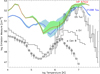 |
Fig. 9 Comparison of plasma emission measure distribution vs. temperature for HIP 67522 and four other G-K stars with different activity levels (see text). A polynomial smoothing (order 2, 0.6 dex in width) was applied to the low and high 1σ boundaries of the EMD solutions for HIP 67522 (Sect. 3.3 and for V 1298 Tau, Maggio et al. 2023). |
Data availability
Supplementary material is available at https://doi.org/10.5281/zenodo.13713288
Acknowledgements
The authors acknowledge partial support by the project Exo- planetary Cloudy Atmospheres and Stellar High energy (Exo-CASH) funded by MUR - PRIN 2022 (grant no. 2022J7ZFRA), and the ASI-INAF agreement 2021-5-HH.0. A.M. also acknowledges support by the project HOT-ATMOS (PRIN INAF 2019). D.L. acknowledges contributions from Bando di Ricerca Fondamentale INAF-MINI-GRANTS di RSN 2 and STILES (Strengthening the Italian leadership in ELT and SKA). This work is based on observations obtained with XMM-Newton, an ESA science mission with instruments and contributions directly funded by ESA Member States and NASA, and on observations made with the NASA/ESA Hubble Space Telescope, obtained from the Space Telescope Science Institute, which is operated by the Association of Universities for Research in Astronomy, Inc., under NASA contract NAS 5–26555. These observations are associated with HST program 16901.
Appendix A Data table
Measured X-ray and FUV line fluxes of HIP 67522.
References
- Barber, M. G., Thao, P. C., Mann, A. W., et al. 2024, AAS Journal, submitted [arXiv:2407.04763] [Google Scholar]
- Batalha, N. M., Rowe, J. F., Bryson, S. T., et al. 2013, ApJS, 204, 24 [Google Scholar]
- Benatti, S., Nardiello, D., Malavolta, L., et al. 2019, A&A, 630, A81 [NASA ADS] [CrossRef] [EDP Sciences] [Google Scholar]
- Bourrier, V., Wheatley, P. J., Lecavelier des Etangs, A., et al. 2020, MNRAS, 493, 559 [Google Scholar]
- Caldiroli, A., Haardt, F., Gallo, E., et al. 2021, A&A, 655, A30 [NASA ADS] [CrossRef] [EDP Sciences] [Google Scholar]
- Caldiroli, A., Haardt, F., Gallo, E., et al. 2022, A&A, 663, A122 [NASA ADS] [CrossRef] [EDP Sciences] [Google Scholar]
- Carleo, I., Malavolta, L., Lanza, A. F., et al. 2020, A&A, 638, A5 [NASA ADS] [CrossRef] [EDP Sciences] [Google Scholar]
- Carleo, I., Desidera, S., Nardiello, D., et al. 2021, A&A, 645, A71 [EDP Sciences] [Google Scholar]
- Cecchi-Pestellini, C., Ciaravella, A., & Micela, G. 2006, A&A, 458, L13 [NASA ADS] [CrossRef] [EDP Sciences] [Google Scholar]
- Chadney, J. M., Galand, M., Unruh, Y. C., Koskinen, T. T., & Sanz-Forcada, J. 2015, Icarus, 250, 357 [Google Scholar]
- Coffaro, M., Stelzer, B., Orlando, S., et al. 2020, A&A, 636, A49 [EDP Sciences] [Google Scholar]
- Cohen, O., Drake, J. J., Glocer, A., et al. 2014, ApJ, 790, 57 [Google Scholar]
- Damasso, M., Lanza, A. F., Benatti, S., et al. 2020, A&A, 642, A133 [EDP Sciences] [Google Scholar]
- Damasso, M., Polychroni, D., Locci, D., et al. 2024, A&A, 688, A15 [NASA ADS] [CrossRef] [EDP Sciences] [Google Scholar]
- Davenport, J. R. A. 2016, ApJ, 829, 23 [Google Scholar]
- Erkaev, N. V., Kulikov, Y. N., Lammer, H., et al. 2007, A&A, 472, 329 [NASA ADS] [CrossRef] [EDP Sciences] [Google Scholar]
- Fortney, J. J., Marley, M. S., & Barnes, J. W. 2007, ApJ, 659, 1661 [Google Scholar]
- Fulton, B. J., & Petigura, E. A. 2018, AJ, 156, 264 [Google Scholar]
- Fulton, B. J., Petigura, E. A., Howard, A. W., et al. 2017, AJ, 154, 109 [Google Scholar]
- Getman, K. V., & Feigelson, E. D. 2021, ApJ, 916, 32 [NASA ADS] [CrossRef] [Google Scholar]
- Heitzmann, A., Zhou, G., Quinn, S. N., et al. 2021, ApJ, 922, L1 [NASA ADS] [CrossRef] [Google Scholar]
- Hudson, H. S. 1991, Sol. Phys., 133, 357 [Google Scholar]
- Husser, T. O., Wende-von Berg, S., Dreizler, S., et al. 2013, A&A, 553, A6 [NASA ADS] [CrossRef] [EDP Sciences] [Google Scholar]
- Ilin, E., Poppenhäger, K., Chebly, J., Ilic, N., & Alvarado-Gómez, J. D. 2024, MNRAS, 527, 3395 [Google Scholar]
- Johnstone, C. P., Bartel, M., & Güdel, M. 2021, A&A, 649, A96 [EDP Sciences] [Google Scholar]
- Kashyap, V., & Drake, J. J. 1998, ApJ, 503, 450 [Google Scholar]
- Kashyap, V., & Drake, J. J. 2000, Bull. Astron. Soc. India, 28, 475 [NASA ADS] [EDP Sciences] [Google Scholar]
- Khodachenko, M. L., Ribas, I., Lammer, H., et al. 2007, Astrobiology, 7, 167 [CrossRef] [Google Scholar]
- King, G. W., Wheatley, P. J., Salz, M., et al. 2018, MNRAS, 478, 1193 [NASA ADS] [Google Scholar]
- Lammer, H., Selsis, F., Ribas, I., et al. 2003, ApJ, 598, L121 [Google Scholar]
- Lammer, H., Lichtenegger, H. I. M., Kulikov, Y. N., et al. 2007, Astrobiology, 7, 185 [NASA ADS] [CrossRef] [Google Scholar]
- Locci, D., Cecchi-Pestellini, C., & Micela, G. 2019, A&A, 624, A101 [NASA ADS] [CrossRef] [EDP Sciences] [Google Scholar]
- Lopez, E. D., & Fortney, J. J. 2013, ApJ, 776, 2 [Google Scholar]
- Lopez, E. D., & Fortney, J. J. 2014, ApJ, 792, 1 [Google Scholar]
- Maggio, A., Flaccomio, E., Favata, F., et al. 2007, ApJ, 660, 1462 [NASA ADS] [CrossRef] [Google Scholar]
- Maggio, A., Locci, D., Pillitteri, I., et al. 2022, ApJ, 925, 172 [NASA ADS] [CrossRef] [Google Scholar]
- Maggio, A., Pillitteri, I., Argiroffi, C., et al. 2023, ApJ, 951, 18 [NASA ADS] [CrossRef] [Google Scholar]
- Mantovan, G., Malavolta, L., Locci, D., et al. 2024, A&A, 684, L17 [NASA ADS] [CrossRef] [EDP Sciences] [Google Scholar]
- Mayor, M., & Queloz, D. 1995, Nature, 378, 355 [Google Scholar]
- Modirrousta-Galian, D., Locci, D., & Micela, G. 2020, ApJ, 891, 158 [Google Scholar]
- Namekata, K., Sakaue, T., Watanabe, K., et al. 2017, ApJ, 851, 91 [Google Scholar]
- Neupert, W. M. 1968, ApJ, 153, L59 [NASA ADS] [CrossRef] [Google Scholar]
- Owen, J. E., & Lai, D. 2018, MNRAS, 479, 5012 [Google Scholar]
- Owen, J. E., & Wu, Y. 2013, ApJ, 775, 105 [Google Scholar]
- Owen, J. E., & Wu, Y. 2017, ApJ, 847, 29 [Google Scholar]
- Pillitteri, I., Argiroffi, C., Maggio, A., et al. 2022, A&A, 666, A198 [NASA ADS] [CrossRef] [EDP Sciences] [Google Scholar]
- Reale, F. 2007, A&A, 471, 271 [NASA ADS] [CrossRef] [EDP Sciences] [Google Scholar]
- Reale, F. 2014, Liv. Rev. Sol. Phys., 11, 4 [Google Scholar]
- Redfield, S., & Linsky, J. L. 2000, ApJ, 534, 825 [NASA ADS] [CrossRef] [Google Scholar]
- Rizzuto, A. C., Newton, E. R., Mann, A. W., et al. 2020, AJ, 160, 33 [Google Scholar]
- Sanz-Forcada, J., Micela, G., Ribas, I., et al. 2011, A&A, 532, A6 [NASA ADS] [CrossRef] [EDP Sciences] [Google Scholar]
- Sanz-Forcada, J., López-Puertas, M., Nortmann, L., & Lampón, M. 2022, in The 21st Cambridge Workshop on Cool Stars, Stellar Systems, and the Sun, Cambridge Workshop on Cool Stars, Stellar Systems, and the Sun, 138 [Google Scholar]
- Scelsi, L., Maggio, A., Micela, G., Briggs, K., & Güdel, M. 2007, A&A, 473, 589 [NASA ADS] [CrossRef] [EDP Sciences] [Google Scholar]
- Serio, S., Reale, F., Jakimiec, J., Sylwester, B., & Sylwester, J. 1991, A&A, 241, 197 [NASA ADS] [Google Scholar]
- Wilms, J., Allen, A., & McCray, R. 2000, ApJ, 542, 914 [Google Scholar]
The epatplot task allows us to test the presence of pile-up on each instrument, starting from unfiltered events of MOS/pn. For the spectrum in interval 2 (first flare peak), the nominal model of single/double pn events in the range 0.5–2.0 keV resulted in agreement with the observed distribution to better than 0.5%. Following the SAS guide, this means no significant pile-up was recorded even during the intervals with the highest source count rate.
For HIP 67522 we adopted a radius of 1.38 R⊙ (Rizzuto et al. 2020).
All Tables
All Figures
|
Fig. 1 X-ray and NUV light curves of HIP 67522. Top: light curves of EPIC (black pn, dark and light blue MOS 1,2) and OM (green) instruments. The EPIC light curves were binned at 600 s per bin, while the OM light curve was binned at 90 s. The OM rate is divided by 5 for making easier the comparison. The horizontal bars on the top indicate the time of the HST/COS exposures. The top axis reports the orbital phases of the planet. The vertical dotted lines mark ingress and midtransit times of the planet. Bottom: EPIC light curves and time intervals defining flares 1 and 2 rise+peak and decay (2, 3, 5, 6) and quiescent levels (1, 4, 7). The gray light curve refers to background single events with energies between 10 keV and 12 keV, in the full field of view of the pn detector. |
| In the text | |
|
Fig. 2 EPIC and RGS global spectra, and best-fit 3T VAPEC model. Black and red data points for the MOS1 and MOS2, while the pn spectrum is in green, and the summed RGS1+RGS2 spectra in blue. The main complexes of H-like and He-like ions are indicated. |
| In the text | |
|
Fig. 3 RGS spectrum of the full exposure, with the identifications of the most prominent emission lines. |
| In the text | |
|
Fig. 4 Spectra of HIP 67522 obtained with COS and grism G130M (central wavelength 1291 Å). Top: FUVB segment (~1140–1280 Å). Bottom: FUVA segment (~1290–1420 Å). The main lines are labeled. |
| In the text | |
|
Fig. 5 Element abundances versus first ionization potential from the global fitting of the EPIC+RGS spectra with a 3T model, and from the emission measure analysis of the COS and RGS line fluxes. |
| In the text | |
|
Fig. 6 Results of the joint analysis of XMM-Newton/RGS and HST/COS spectra. Top: Plasma EMD vs. temperature, compared with the 3-T model (red points) best fitting the global EPIC and RGS spectra. The shaded band represents a smoothed 1σ confidence region. Bottom: differences, in σ units, between measured line fluxes and predicted values vs. temperature at the peak emissivity. The black “H” symbols represent narrow-band measurements of the X-ray continuum. Empty symbols are lines not used for the EMD reconstruction. |
| In the text | |
|
Fig. 7 X-ray vs. EUV scaling laws and benchmark stellar sample. (Left) Measurements of the EUV to X-ray ratio vs. X-ray flux at the stellar surface for HIP 67522, the Sun, and other G-K-type stars. The names indicate benchmark stars with exoplanets. Different X-ray (5–100 Å) to EUV (100–920 Å) scaling laws are shown for comparison: the gray band indicates the 90% confidence region relative to the J21 scaling law (green dashed line). The golden band is the 90% confidence region for the SF22 scaling law, assuming stars with radii equal to that of HIP 67522, while the orange band is for stars with 0.7 R⊙. The ranges for the Sun indicate its variability during an entire magnetic cycle. (Right) Analogous plot for the scaling laws of the EUV vs. X-ray luminosities. The gold dashed lines represent an extrapolation of the SF22 solution, while the gray-shaded area comprises stars with radii in the range 0.7–1.38 R⊙. |
| In the text | |
|
Fig. 8 Composite spectrum of HIP 67522 obtained by joining the Phoenix photospheric spectrum with the XUV spectrum synthesized from the reconstructed plasma emission measure distribution vs. temperature in the chromosphere, transition region, and corona. The upper panel shows the specific flux at Earth, while the bottom panel is the photon flux at a distance of 1 AU. The Phoenix spectrum resampled down to ~1700 Å with a wavelength resolution of 1 Å is shown in green; the XUV spectrum in the range 1–1700 Å is shown instead with a resolution of 0.01 Å. The green and blue segments in the upper panel, at ~200 nm, mark the Phoenix model flux and the observed flux integrated over the OM UVM2 band. |
| In the text | |
|
Fig. 9 Comparison of plasma emission measure distribution vs. temperature for HIP 67522 and four other G-K stars with different activity levels (see text). A polynomial smoothing (order 2, 0.6 dex in width) was applied to the low and high 1σ boundaries of the EMD solutions for HIP 67522 (Sect. 3.3 and for V 1298 Tau, Maggio et al. 2023). |
| In the text | |
Current usage metrics show cumulative count of Article Views (full-text article views including HTML views, PDF and ePub downloads, according to the available data) and Abstracts Views on Vision4Press platform.
Data correspond to usage on the plateform after 2015. The current usage metrics is available 48-96 hours after online publication and is updated daily on week days.
Initial download of the metrics may take a while.