| Issue |
A&A
Volume 666, October 2022
|
|
|---|---|---|
| Article Number | A198 | |
| Number of page(s) | 10 | |
| Section | Stellar structure and evolution | |
| DOI | https://doi.org/10.1051/0004-6361/202244268 | |
| Published online | 26 October 2022 | |
X-ray flares of the young planet host Ds Tucanae A
1
INAF-Osservatorio Astronomico di Palermo, Piazza del Parlamento 1, 90134 Palermo, Italy
e-mail: This email address is being protected from spambots. You need JavaScript enabled to view it.
2
Università degli Studi di Palermo, Piazza Marina 61, 90133 Palermo, Italy
3
Harvard-Smithsonian Center for Astrophysics, 02138 Garden St, Cambridge, MA, USA
Received:
14
June
2022
Accepted:
15
August
2022
Abstract
The discovery of planets around young stars has spurred novel studies of the early phases of planetary formation and evolution. Stars are strong emitters at X-ray and UV wavelengths in their first billion of years and this strongly affects the evaporation, thermodynamics, and chemistry in the atmospheres of the young planets orbiting around them. In order to investigate these effects in young exoplanets, we observed the 40 Myr old star DS Tuc A with XMM-Newton. We recorded two X-ray bright flares, with the second event occurring about 12 ks after the first one. Their duration, from the rise to the end of the decay, was about 8 − 10 ks in soft X-rays (0.3–10 keV). The flares were also recorded in the 200–300 nm band with the UVM2 filter of the Optical Monitor. The duration of the flares in UV was about 3 ks. The observed delay between the peak in the UV band and in X-rays is a probe of the heating phase, followed by evaporation and an increase in the density and emission of the flaring loop. The coronal plasma temperature at the two flare peaks reached 54–55 MK. Diagnostics based on the temperatures and timescales of the flares applied to these two events have allowed us to infer a loop length of 5 − 7 × 1010 cm, which is about the extent of the stellar radius. We also inferred the values of electron density at the flare peaks of 2.3 − 6.5 × 1011 cm−3, along with a minimum magnetic field strength on the order of 300–500 G that is needed to confine the plasma. The energy released during the flares was on the order of 5 − 8 × 1034 erg in the bands 0.3 − 10 keV and 0.9 − 2.7 × 1033 erg in the UV band (200–300 nm). We speculate that the flares were associated with coronal mass ejections (CMEs) that hit the planet about 3.3 h after the flares, which dramatically increased the rate of evaporation for the planet. From the RGS spectra, we retrieved the emission measure distribution and the abundances of coronal metals during the quiescent and flaring states, respectively. Finally, we inferred a high electron density measurement, which is in agreement with the inferences drawn from time-resolved spectroscopy and EPIC spectra, as well as the analysis of RGS spectra during the flares.
Key words: stars: activity / stars: coronae / X-rays: stars / stars: flare
© I. Pillitteri et al. 2022
 Open Access article, published by EDP Sciences, under the terms of the Creative Commons Attribution License (https://creativecommons.org/licenses/by/4.0), which permits unrestricted use, distribution, and reproduction in any medium, provided the original work is properly cited.
This article is published in open access under the Subscribe-to-Open model. This email address is being protected from spambots. You need JavaScript enabled to view it. to support open access publication.
1. Introduction
X-rays are emitted by solar type stars during their early evolution (Vaiana et al. 1981; Pallavicini et al. 1981; Feigelson & Montmerle 1999) and they serve as a powerful proxy for the structure of the stellar coronae and magnetic fields that confine the hot coronal plasma. Over their first hundred million years, solar-type stars exhibit very high magnetic and coronal activity, as well as high stellar rotation rates (Pizzolato et al. 2003). The loss of angular momentum during the main sequence is accompanied by a decrease in the X-ray luminosity by a factor of 103 during the first billion years (Pallavicini et al. 1981; Vaiana et al. 1981; Favata et al. 2003).
Interest in studying the activity of stars at high energies has been renewed thanks to recent discoveries of extrasolar planets. High-energy photons and particles can affect planetary atmospheres and their potential habitability. Fluxes at high energies (X-rays and EUV, XUV) have a strong role in shaping and transforming the primary atmospheres of the planets and their evaporation. Because of the decrease in stellar activity, most of the effects due to XUV irradiation are expected to take place in the first Gyr (Penz & Micela 2008; Cecchi-Pestellini et al. 2009; Kubyshkina et al. 2018). Collectively, the action of the magnetized stellar winds and the coronal mass ejections (CMEs) can make the planets lose a significant fraction of their atmospheres and change their compositions through photo-chemical processes (see Drake et al. 2013; Kay et al. 2019, and references therein). However, the effects of the sudden and violent release of energy during flares and CMEs onto the planets are still poorly understood due to the lack of proper monitoring of the stellar coronae required in order to build a reliable distribution of flaring rates versus age and of adequate time-resolved modeling of the dynamics and chemistry of the planetary gaseous envelopes. In this context, the study of young stars hosting planets, such as DS Tuc, in the X-ray and UV bands is of utmost\relevance.
DS Tuc is composed of a pair of two young stars at a distance of 44.1 pc from the Sun, with an age of ∼40 Myr and exhibiting spectral types G6 (component A and host of the planet) and K3 (component B). The planet around DS Tuc A was independently discovered in NASA TESS observations (TOI-200) by Benatti et al. (2019) and Newton et al. (2019). DS Tuc Ab has a radius of 0.5RJ, a mass upper limit of 14.4 M⊕ (Benatti et al. 2021) and orbits its host star in 8.14 days. These characteristics suggest a very low density for the planet and that it is prone to strong atmospheric evaporation. This is one of few very young planets discovered so far. Its properties can serve to test models of dynamical and atmospheric evolution. For the purpose of investigating its coronal emission, DS Tuc has been observed with XMM-Newton in two different epochs. In Benatti et al. (2021), we presented an analysis and a description of the global properties of the coronae of the system of DS Tuc and we related the X-ray emission to a model of the atmospheric evaporation occurring during the main sequence.
In the optical band, TESS observed DS Tuc A in six sectors, allowing Colombo et al. (2022) to perform a reconstruction of the distribution of the optical flares and their main properties (see also Howard 2022). They also inferred the energies of the X-ray counterparts of TESS flares through the scaling laws of Flaccomio et al. (2018) before X-rays observations were available. Here, we study two bright flares of DS Tuc A and discuss their impact on the atmosphere of DS Tuc Ab.
This paper is structured as follows: Sect. 2 describes the observations and the data analysis, Sect. 3 presents our results, and Sect. 4 contains our discussion and conclusions.
2. XMM-Newton observations and data analysis
DS Tuc has been observed twice in the X-ray band with XMM-Newton during observations ObsId = 0863400901 (P.I. S. Wolk) and 0864340101 (P.I. A. Maggio) with exposure times of about 40 ks and 30 ks, respectively. Based on the first observation (Benatti et al. 2021), we measured X-ray fluxes and luminosities of the pair of stars of DS Tuc A and B, separated by ∼5.3″ and partially resolved in MOS detectors. The A component was 1.3 times more luminous in X-rays than DS Tuc B. We also inferred a mean coronal temperature and emission measure of both stars. Some degree of variability in form of flares was observed in DS Tuc B while DS Tuc A was quieter. From these, we estimated the timescale of the evaporation of DS Tuc Ab and the evolution of its mass and radius in the next 5 Gyr.
The second observation of DS Tuc with XMM-Newton was performed on April 11th 2021 (obsId 0864340101)1, again with EPIC as main instrument. We adopted the Medium filter and the SmallWindow mode for both MOS and pn. In addition, we acquired simultaneous high resolution spectra with the Reflection Grating Spectrometer (RGS) and a light curve in the band 200 − 300 nm with the Optical Monitor (OM), using the UVM2 filter in fast mode. For the OM, we obtained five continuous exposures of 4400 s and one exposure of 3880 s, and for each exposure, a light curve with a time binning of 10 s was obtained.
The ODFs files downloaded from the XMM-Newton archive2 were reduced with SAS version 18.0.0 to obtain event tables for EPIC instruments, light curves for the OM, and spectra for the two RGS high-resolution spectrometers. We selected the EPIC events for having energies in the band 0.3 − 10.0 keV and FLAG == 0 and PATTERN < = 12, as prescribed by the SAS reduction guide. We checked that the overall background was low during the observation, thus the full exposure was retained for further analysis. A visual inspection of the pn and MOS images revealed that DS Tuc A had undergone strong flaring activity and its flux dominated the emission of the nearby DS Tuc B. In Fig. 1, we show two MOS1 images relative to two different time intervals and referring to the quiescent and flare peak intervals of DS Tuc A.
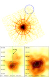 |
Fig. 1. XMM-Newton images of the DS Tuc system. Top panel: MOS 2 image of DS Tuc with the regions used for accumulating source and background events. The scale is logarithmic to enhance the background level otherwise not visible on a linear scale. The background region was offset to one of the corner of the chip to avoid the diffraction spikes from the central source. Bottom left: image of MOS 1 during the first 6 ks of observation and corresponding to interval 1 in Fig. 2. We marked the SIMBAD positions (J2000) of DS Tuc A and B and the vectors of proper motions. Bottom right: image during interval 3 corresponding to the peak of the first flare. In both images, the scale limits and color maps are identical, the binning is 8 pixels corresponding to ∼0.4″ and a smoothing with a Gaussian with σ = 1.5 pixels has been applied to images. We added contour levels with the same ranges for marking the source centroid. |
The spectra and light curves of DS Tuc A were obtained from events in a circular region of radius 75″ centered on the X-ray image centroid (see Fig. 1). The spectra of the background were accumulated from an offset circular region of radius 45″. Given the brightness of DS Tuc A in this observation, we checked for any pile up that could have affected the spectra of MOS and pn. We generated the pattern of single, double, triple, and quadruple events as a function of the energy, as prescribed by the SAS guide. The diagnostic modeling of the curve did not show evidence of significant pile-up, so we retained the entire list of events in the region.
The high count statistics recorded in the EPIC instruments allowed us to perform a time-resolved spectroscopy study of the two flares. To this end, we accumulated the spectra in 13 time intervals that define the initial quiescent state, the flare rises, peaks, and decays (see Fig. 2). For each time interval, the spectra of the source and the background were created with SAS, along with the corresponding response matrices and effective area ARF files.
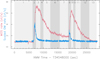 |
Fig. 2. Light curves of MOS 1 (red curve, bin size 150 s) and OM in the UVM2 filter (blue curve, bin size 10 s). The OM rate is scaled down by a factor 30 to allow a direct comparison of the rise and decay times of both instruments during the flares. The time intervals used for time resolved spectroscopy (see Sect. 3.2) are indicated by the alternating light or dark gray areas and numbered on top of each panel. |
For the OM, we obtained five exposures of 4400 s and one of 3880 s. In each exposure, a light curve with time binning of 10 s was accumulated with the standard SAS task omfchain, with the result displayed in Fig. 2. For extracting the RGS spectra, we used the SAS task rgsproc and rgscombine, with custom good time intervals defined as interval 1 for the quiescent phase and 2–13 for flares. We summed the RGS spectrum of the first XMM-Newton observation (ObsId 0863400901) with the spectrum of the quiescent interval 1, since both are representative of a quiescent phase or at least with low level of variability. Furthermore, we added RGS 1 and RGS 2 spectra of the quiescent and flaring phases for achieving a better count statistics.
3. Results
Here, we discuss the quiescent emission and the flaring emission observed in the present observation individually.
3.1. Quiescent phase
The quiescent interval before the first flare was about 6.5 ks with an average rate of 0.9 ct/s in MOS1, this interval served to estimate the coronal plasma properties before the ignition. We used a sum of 3 APEC thermal components plus a global absorption to model the EPIC spectra and obtain a statistically satisfactory description of the spectrum. Table 1 lists the best-fit parameters and Fig. 3 shows the spectrum during time interval 1 and 3 for comparison. We performed the best-fit procedure to each EPIC spectrum and jointly as well, obtaining very similar results.
Best fit parameters of the 3T model for the quiescent spectrum observed during interval 1.
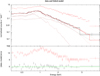 |
Fig. 3. Spectra of MOS 1 relative to the time intervals 1 (black line and crosses) and 3 (red crosses). The best fit model to the spectrum of the plasma during interval 1 with its 3 component is shown along with the χ residuals in the bottom panel. |
The main thermal component of the quiescent spectrum is log(T/K) ∼ 7.02, with the addition of a soft component log T/K ∼ 0.54 and a hotter component that is much less constrained, log T/K ≥ 7.4. By setting a fixed very low value to the equivalent column of gas absorption (NH = 8 × 1018 cm−2), we can constrain the hot component at around log T ∼ 7.4 (90% confidence range: 7.31–7.58), while the other parameters remain unchanged. However, the very low gas absorption is not consistent with the values of visual extinction and reddening.
The temperatures are consistent with the values determined from the analysis of spectra acquired during the first XMM-Newton observation (Benatti et al. 2021). The average flux of DS Tuc A in interval 1 is about 1.9 times the flux observed during the first XMM-Newton observation. However, some degree of contamination from DS Tuc B in this estimate has to be accounted for in the analysis of this first time interval. Visual inspection of the image relative to the events of the quiescent interval shows that DS Tuc A is still the most prominent source and DS Tuc B has a lower count statistics. The contribution to flux of DS Tuc A from its stellar companion DS Tuc B is on the order of 40% during interval 1. After correcting for this contamination fraction, we infer that the quiescent flux of DS Tuc A in interval 1 was about 15% higher than the average X-ray flux measured during the first XMM-Newton observation.
3.2. Flares
We observed two prominent flares after the initial phase of quiescence that lasted for about 6.5 ks (Fig. 2) from the start of the XMM-Newton observation. The second flare occurred about 12 ks after the beginning of the first flare. In Fig. 2, we show a light curve of the OM with scaled count rate to allow a straightforward comparison of the timing of the flares. Each flare starts simultaneously in X-rays and UV, however, in the UV band the flares peak earlier and decays quicker than in X-ray. When the flux reaches each flare peak in UV the rise of the flux in X-rays does flatten while continuing to increase. The peak in UV corresponds to the end of the heating phase during the flares, while the loop continues to be filled with plasma evaporating from its feet – thus increasing the emission measure and the flux in X-rays (Namekata et al. 2017). This timing and shape of the flares in the near UV band and in X-rays is analog to the Neupert effect seen in the Sun (Neupert 1968). Neupert noticed that time-integrated microwave fluxes closely match the rising portions of soft X-ray (SXR) emission. The effect has been demonstrated since in other studies (e.g., Kahler et al. 1988), and later dubbed the “Neupert effect” by Hudson (1991). Estimating the time-integrated microwave fluxes from the non-thermal hard X-ray (HXR) emission, the Neupert effect has been generalized, where the time derivative of the SXR, namely, dFSHXR(t)/dt, can be considered a proxy for the HXR emission FHXR(t) (Dennis & Zarro 1993, Veronig et al. 2002). In our case, near-UV flux measured with OM is a proxy of the dFHXR/dt, with HXR being the emission in 0.3–10 keV probed by EPIC.
In the UV, we measured rise times of 180 ± 5 s and 70 ± 5 s for the first and second flares, respectively. In the X-rays, we measured rise times of 900 ± 75 s and 750 ± 75 s, respectively. The delay between the peak of each flare in UV and X-rays amounts to ∼680 s and ∼930 s, respectively. In a linear-log plane the decay phase of the flares first appear to be linear, meaning that the first part of the decay can be modeled with an exponential relationship between count rate and time; then it indeed flattens, as it deviates from a pure exponential decay. With a linear best-fit modeling to the first part of the decay of both flares in the linear-log plane, we estimated e-folding times of 3.55 ks and 2.31 ks for flares 1 and 2, respectively. With a similar procedure, we determined that in UV, the flare decays are shorter than in X-rays and on the order of 390 s and 375 s for flares 1 and 2, respectively.
The evolution of the plasma temperature and emission measure offers diagnostics that can provide information on the size of the magnetic loop hosting the flare, the presence of prolonged heating, and the minimum magnetic field required to confine the plasma (Reale 2007, 2014). In order to follow the evolution of the flares, we divided the light curve during the flares in 12 intervals that identify the rise, the peak, and the decay (resolved with three different segments apiece) of each flare, as indicated in Fig. 2. For each interval, we modeled the extracted spectra with a sum of a flaring component described by one APEC optically thin plasma thermal emission model added to the 3T model that describes the quiescent emission (cf. Sect. 3.1). We also left the global absorption and the global abundances free to vary. For each time segment, the best-fit parameters of spectra of MOS 1 and 2 and pn are listed in Table 2. We did not perform a joint best-fit to the 3 EPIC spectra of each time interval because the diagnostics of the flares are calibrated for each instrument separately. The absorption is on the order of 1020 cm−2; in a few cases it is not well constrained, but we found the 90% confidence level value to always remain below 4 × 1020 cm−2. These values are in agreement with the estimates of optical extinction towards DS Tuc (cf. Benatti et al. 2021).
Best fit parameters from time resolved spectroscopy of EPIC spectra.
Figure 4 shows the scatter plots of the flare temperatures versus the emission measures (EM) for each EPIC instrument. Points 2–7 refer to the first flare and points 8–13 refer to the second flare (cf. Table 2). In the spectra of MOS 1 and pn, the peak temperatures in both flares are detected in segments 2 and 8 for flare 1 and 2, respectively, and on the order of log T/K ∼ 7.7 − 7.75. In MOS 2, for the second flare the peak temperature is detected in segment 9, however its value is consistent with what was measured in segment 8 with the other two instruments. The peaks of EM are reached in segments 3 and 9 for MOS 1 and pn with values of logEM(cm−3)≈54. Owing to our choice of the time intervals, the peak of EM in MOS 2 is seen in segment 8 instead of 9, but still consistent with the values determined from MOS 1 and pn. We inferred a metallicity value of Z between 0.2 during the decay and 0.5 at the flare peaks.
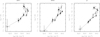 |
Fig. 4. Log T (MK) vs. E.M. during the evolution of the two flares. Left panel: log T and E.M. derived from MOS1 spectra. Central panel: values derived from the MOS2 spectra. Right panel: parameters derived from pn spectra. Solid symbols refer to the first flare, open symbols refer to the second flare, and numbers refer to the time intervals. The error bars mark the 90% confidence interval. |
The slopes between points 3 and 7 and then 9–13 in the log T/EM plane, the temperatures at the peaks of the flares, and the e-folding time of the decay of the flares can be used to infer the size of the loops that hosted the flares, using the diagnostics of Reale (2007, 2014). Table 3 shows the slopes derived for each flare and EPIC instrument, the total loop lengths, the estimates of the electron densities, and the minimum strength of the magnetic field required to constrain the plasma in the loop at the peak of both flares. We inferred a full loop length on the order of the stellar radius (5 − 7 × 1010 cm). To estimate the electron density we first calculated the volume of the flaring loops assumed as tubes with a ratio between base radius and length of 0.1. Then we derived the electron densities from E.M., as  (Maggio et al. 2000). Electron densities at the flare peaks are found to be on the order of 2 − 6.5 × 1011 cm−3. We can also infer the minimum strength of the magnetic field needed to confine the plasma to be (from e.g., Maggio et al. 2000):
Slope in the plane log T vs. log EM/2 (ξ), loop length, electron density and minimum magnetic field derived for the first and second flare for each EPIC instrument.
where kB is the Boltzmann’s constant and ne, peak and Tpeak are the density and the temperature at the flare peak. We estimated a minimum magnetic field between 300 G and 500 G.
3.3. RGS lines
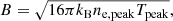
We analyzed the first-order RGS spectra of both XMM-Newton observations to infer the emission measure distribution (EMD), abundances, and electron density of the X-ray emitting plasma during the quiescent and flaring phases (Fig. 5). First order RGS spectra cover the range ≈4 − 38 Å with a resolution 0.06 Å FWHM. The exposures of the quiescent and flaring intervals have a duration of 45.53 ks and 22.15 ks, respectively. The quiescent spectrum was accumulated by summing up the events collected during the whole first XMM-Newton observation and the first 6.2 ks of the present observation. For the flaring phase, we considered the remaining 22.2 ks encompassing the two flares altogether. The RGS spectra of the first order are made of 11 200 and 20 700 net counts, respectively. For the analysis of the RGS data, we used the IDL package PINTofALE, (Kashyap & Drake 2000) and the XSPEC v12.11b software (Arnaud 1996). For the line emissivities, we adopted the CHIANTI atomic database (v7.13, Dere et al. 1997).
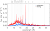 |
Fig. 5. RGS spectra corresponding to quiescent and flaring phases. The identifications of some of the strongest lines are reported on top. For clarity, the two spectra have been slightly smoothed. |
We identified the strongest emission lines and measured their fluxes by fitting the RGS spectra in small wavelength intervals of ∼1.0 Å width. The width of each wavelength interval is set to include and, hence, to simultaneously fit the blended lines. Each observed line was fit assuming that its shape is fully described by the RGS line spread function (the intrinsic width of coronal emission lines is expected to be negligible compared to the RGS line spread function). For each wavelength window encompassing the lines we meant to fit, we took into account the continuum contribution in the best-fit procedure, leaving the temperature and normalization as free parameters. Given the small width of each wavelength window, the continuum component from the best fit acts as an additive constant value. This additive constant contribution, mimicking the apparent continuum level, ensures that the contributions of unresolved small lines and wings of other strong lines in the vicinity are taken into account. The measured line fluxes are listed in Table 4. In the case of spectral features suspected to be due to the blend of more than one line, we listed the different ions contributing to the observed flux.
Measured fluxes of emission lines and continuum intervals in the X-ray spectrum of DS Tuc.
To determine absolute abundances and EMD values and to better constrain the hottest components of the EMD, continuum flux measurements are also needed. The continuum flux level obtained within the line fitting procedures is often an overestimate of the real continuum level, because of the significant contribution of small unresolved lines, which is known to affect large portions of the RGS wavelength range. Therefore, to obtain reliable measurements of the continuum, we selected small wavelength intervals where line contamination is known to be minimal (on average less than 10%). The continuum flux measurements in these intervals were obtained by integrating the observed net counts. The total emissivity function associated to these continuum measurements was nonetheless computed with the inclusion of the small fraction of the emission line contribution in addition to the continuum one. The selected intervals and the corresponding measured fluxes are listed in Table 4.
We derived the EMD and the abundances corresponding to the quiescent and flaring phases by applying the Markov chain Monte Carlo method from Kashyap & Drake (1998). Flux measurements used for the EMD reconstruction are listed in Table 4. We discarded density-sensitive lines and lines whose fluxes are highly uncertain because of strong blending. Measured fluxes were first converted into unabsorbed fluxes assuming a hydrogen column density of NH = 2 × 1020 cm−2; this is an average value inferred from the analysis of EPIC spectra (cf. Sect. 3.1) and from that reported by Benatti et al. (2021). Given the range of formation temperatures of the measured fluxes, we reconstructed the EMD over a regular logarithmic temperature grid, with bins of width of 0.10 dex, encompassing the range of log T(K) from 6.0 to 8.0 dex. We show in Fig. 6, the emissivity functions associated with the line and continuum flux measurements used for the EMD derivation. The hot tails that characterize the shapes of the emissivity functions of several lines, as well as that of the continuum intervals, make their associated flux measurements highly sensitive to the amount of hot plasma components. Moreover, since we used both line and continuum flux measurements to reconstruct the EMD, the inversion procedure simultaneously provides the absolute abundances for those elements for which at least one line has been measured. For the measured spectral features that include lines of different elements, the total emissivity that is needed for the EMD reconstruction depends on the starting abundance values of the elements involved. For this reason, the EMD and abundance reconstruction were performed recursively. The first attempts of EMD reconstruction indicated that the abundances of the quiescent and flaring phases do not differ significantly from each other. Because of this, in the final EMD derivation of the quiescent phase we assumed the same set of abundances obtained from the analysis of the flaring phase, where, due to the higher line fluxes, they are determined with a better level of precision. The EMD and the abundances derived for the X-ray emitting plasma of DS Tuc A are reported in Table 5. The two EMDs are also plotted in Fig. 7.
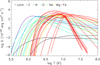 |
Fig. 6. Emissivity functions of the ion lines (colored curves) and continuum (black curves) measured in RGS spectra. |
EMD and abundances of DS Tuc.
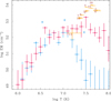 |
Fig. 7. EMDs derived from the RGS line fluxes for the quiescent (blue) and flaring phases (red). Asterisks and solid points mark the EM derived from EPIC detectors for the quiescent (blue symbol, 3T APEC) and flaring intervals, (red symbols and interval numbers, 1T APEC). |
It is possible to constrain the X-ray emitting plasma density, ne, by inspecting the diagnostics provided by He-like line triplets and other density-sensitive line ratios. Among the emission lines detected in the flaring and quiescent RGS spectra, density-sensitive line ratios are provided by the He-like triplets of Mg XI (resonance r at 9.17 Å, intercombination i at 9.23 Å, forbidden f at 9.31 Å), Ne IX (λr = 13.45 Å, λi = 13.55 Å, λf = 13.70 Å), and O VII (λr = 21.60 Å, λi = 21.81 Å, and λf = 22.10 Å), and by the pair of Fe XVII lines at 17.05Å and 17.10 Å (Mauche et al. 2001).
However, we did not analyze the He-like Ne IX triplet at ∼13.5 Å, because of its severe blending with strong Fe lines makes its measured fluxes highly uncertain. The O VII triplet, which has a maximum formation temperature of ∼2 MK, allows us to measure the density of relatively cold coronal plasma. The Mg XI and Fe XVII density diagnostics instead probe hotter plasma components, since their line maximum formation temperatures are at ∼6 MK.
The f/i line ratio of the O VII triplet is high and compatible with the low density limits for both the quiescent and flaring phases. Density sensitive lines of Mg XI and Fe XVII, of the quiescent and flaring phases, are displayed in Fig. 8. Both the quiescent and flaring spectra in the Mg XI region are quite noisy due to the low signal-to-noise ratio (S/N) of the lines and to the significant continuum emission in this region, especially during flares. The Fe XVII lines are well exposed, with a good S/N ratio in both the quiescent and flare spectra. However, the Fe XVII lines are separated by 0.05 Å, which is comparable with the RGS spectral resolution (0.06 Å) and which makes the two lines only marginally resolved. Because of all these sources of uncertainty, the Mg XI and Fe XVII line fluxes were obtained by freezing line positions, leaving the line fluxes as free parameters for the best fits of the line profiles.
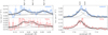 |
Fig. 8. Observed (histogram with error bars) and best fit (solid black curve) spectra of the quiescent and flaring phases in the regions of the Mg XI triplet and Fe XVII density sensitive lines. Best-fit functions corresponding to individual line are also shown with solid grey lines. Left panels show r, f, and i labels, indicating the resonance, inter-combination, and forbidden lines of the Mg XI triplet. |
The observed f/i ratio of Mg XI and the F(17.10)/F(17.05) ratio of Fe XVII change significantly during the quiescent and flaring phases. During quiescent emission, both Mg XI and Fe XVII have both ratios compatible with the low density limit: f/i > 2 and  , both indicating ne < 1013 cm−3. Conversely, during the flaring phases, both ratios decrease significantly (
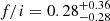 and F(17.10)/F(17.05)=0.16 ± 0.07), indicating a high plasma density (ne ∼ 1014 cm−3), as shown in Fig. 9. This value is derived from relatively cold lines which probe the cooler plasma in the loop, namely, toward its feet (Argiroffi et al. 2019). Conversely, the plasma density inferred from the emission measure and the loop volume described in Sect. 3.2 is valid for hotter plasma towards the apex of the loop during the flare peak. Also, in deriving the electron density from the flare emission measure, the choice of the volume has some degree of arbitrariness.
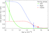 |
Fig. 9. Predicted line ratios:f/i for O VII and Mg XI and F(17.10)/F(17.05) for Fe XVII) computed at different plasma densities, together with the observed line ratios observed during the flaring phase. |
The abundances of elements inferred from the line fluxes, scaled to the values of the solar photosphere as a function of first ionization potential (FIP), are reported in Fig. 10. Apart from the high uncertainty of the abundance of C, a trend with FIP is visible with Fe and Mg (as well as perhaps O) being under abundant, owing to their low FIP. The trend is in agreement with the inverse-low FIP effect observed in active stars.
 |
Fig. 10. Ratio AX/AX⊙ vs. first ionization potential derived from the abundances analysis of RGS spectra |
4. Discussion and conclusions
In this paper, we present an analysis of an XMM-Newton observation of DS Tuc A, one of the youngest known planet hosts. DS Tuc Ab is an inflated planet with a radius of about 0.5RJ and with mass less than 14.4 M⊕ that will likely shrink to a size of about 2 R⊕ in the next hundreds of Myr (Benatti et al. 2021). Observations in X-rays are important to understand the processes that can modify both dynamics and chemistry of the primary atmospheres of newly born planets. In this context, the present work allows for a deep characterization of the coronal emission and time variability of the star and its effects on its close-in planet. We detected two bright flares in DS Tuc A that permitted a time-resolved spectroscopy of the two events. The energy released during the first and second flare are about 8 × 1034 erg and 5 × 1034 erg.
Colombo et al. (2022) used TESS light curves of DS Tuc to study the rate of flares of DS Tuc in the optical band with an analysis of all available sectors through an iterative method that is based on Gaussian processes. These authors found that the frequency of flares with energy (in optical band) larger than 2 × 1032 erg amounts to about two per day. A similar result was obtained by Howard (2022). By using the relationship between flare energy released in the optical band and in X-rays inferred by Flaccomio et al. (2018) from the flares observed in the NGC 2264 young star-forming region, this limit corresponds to X-ray energies on the order of 1031 erg. The flares we detected in the present XMM-Newton observation seem very rare events that are likely to have released energies in the optical band in excess of 5 × 1035 erg, which comprises the very high energy tail of the flare energies observed with TESS by Colombo et al. (2022). Furthermore, in the optical band, there is a significant fraction of pairs of flares separated by a few ks, similarly to the separation of the two flares that we observed in X-rays. The cause could be a triggering mechanism of the same active region after the first flare has been ignited in a scenario where the corona is densely packed with magnetic structures that are somehow interacting with each other. The UV energy of the flares was calculated from the count rates and the conversion factor for the UVM2 filter (assuming a band width of 100 Å) in the case of a WD at 10 000 K3. These energies amount to 2.7 and 0.9 × 1033 erg for flares 1 and 2, respectively, and result in energies that are a factor of 30–50 lower than those released in the X-ray band.
In the pre-main sequence stars of Orion, X-ray flares that release energies of ≥5.5 × 1035 erg constitute the upper 50% of the sample of the bright flares observed in COUP (cf. Fig. 9 in Wolk et al. 2005). It is plausible that the frequency of such energetic events decreases between the age of young pre-main sequence stars in Orion (3 − 5 Myr) and the age of DS Tuc, about 40 Myr.
With an age of 40 Myr, the X-ray activity of DS Tuc A is observed to have just started its decline in the main sequence phase and can be probed by a value of the ratio log LX/Lbol ∼ −3.55 (Benatti et al. 2021). The average X-ray luminosity of DS Tuc A in this observation was 9.1 × 1030 erg s−1, which is about a factor of 10 higher than recorded in the first XMM-Newton observation (Benatti et al. 2021). During these flares, the ratio log LX/Lbol reached the value of ≈ − 2.15 or ≈0.7% of its bolometric luminosity.
From the ephemeris established by Benatti et al. (2019), we estimated that the planet was at the orbital phases ϕ between ∼ − 0.06 and ∼ − 0.11 during this observation (with ϕ = 0 as the phase of the transit and ∼ − 0.008 the phase of the first contact) and, thus, the planet was observed between 19 and 12 hours before the transit. The stellar rotation period is about 2.9 days, which amounts to ≈250.5 ks, and so, the present XMM-Newton exposure covered about 12% of the rotation period. The flares did not show any dimming due to self-eclipse and so, we infer that either they occurred in active regions near the equator and in the central portion of the stellar disk or the active regions were at very high stellar latitudes and coronal loops with sizes similar to the stellar radius anchored at high stellar latitudes could be visible even when the feet of the loops are behind the visible disk.
The values of peak luminosity are about 1.8 × 1031 erg s−1, corresponding to a flux of about 100 erg s−1 cm−2 at the surface of the planet, which is on the order of 0.1 W m−2. Conversely, the X-ray flux received by the planet from the quiescent star is about 0.01 W m−2. An hypothetical Earth around DS Tuc A at 1 AU would have received 6.3 × 10⁻⁴ W m−2 in the band 0.3 − 10 keV, which corresponds to a GOES X6 flare in the band 1 − 8 Å. We speculate that CMEs were associated with those flares. Drake et al. (2013; see also Osten & Wolk 2015; Moschou et al. 2019) have given an estimate of the mass and kinetic energy associated with powerful flares observed in the Sun. From their Eq. 1, which relates to young stellar coronae in the saturated regime as in the case of DS Tuc A, we estimated that the mass associated with CMEs was around 5 × 10⁻¹⁵ M⊙. We also infer that the kinetic energy associated with the CMEs is ≈1034 erg. From these numbers, we can also infer a velocity of the CME material on the order of 1000 km s−1. With these velocities, the CME would have reached DS Tuc Ab in about 3.3 h after the ignition of the flares. Simulations of CMEs hitting close-in planets at a few stellar radii from their stars (see Alvarado-Gómez et al. 2022; Hazra et al. 2022) demonstrate that the CMEs associated with the flares could be even more disruptive for the outer atmosphere, resulting in dramatic changes of the rate of evaporation with respect to the effect of a steady stellar wind or from X-ray irradiation alone in the aftermath of a flare.
The RGS spectra have enabled us to reconstruct the emission measure distribution (EMD) for the quiescent and flaring states. The EMDs are very similar, with values in the range of 6 < log T < 7.1, whereas they differ significantly above log T > 7.1, with the maximum difference occurring at log T ≈ 7.5. The difference is due to the dense plasma heated during the flares. The integral of the difference between the flare and quiescent phase EMDs within a range of temperatures, 7 < log T < 8, amounts to logEM ≈ 53.5; this is consistent, on average, with the values inferred from the time resolved spectroscopy of EPIC spectra. Qualitatively, hard X-rays produced during the flares can penetrate more deeply in the planet’s atmosphere, along with a cascade of electrons that induce further dissociation and photochemistry. Such a mechanism may be nonlinear if the atmosphere is unable to restore its state before the next flare. Louca et al. (2022) modeled the response of several planetary atmospheres to flares, determining the conditions under which the initial conditions are restored and the consequent enhancement of several species is facilitated. In this respect, a more systematic X-ray monitoring of stars with close in planets would be beneficial for improving the general understanding of the formation and evolution of planetary atmospheres.
A detailed log of the observation is available at: https://xmmweb.esac.esa.int/cgi-bin/xmmobs/public/obs_view.tcl?search_obs_id=0864340101
Acknowledgments
We thank the anonymous referee for their useful comments and suggestions that improved the quality of this manuscript. I.P., A.M., S.C. and G.M. acknowledge financial support from the ASI-INAF agreement n.2018-16-HH.0, and from the ARIEL ASI-INAF agreement n.2021-5-HH.0. S.J.W. was supported by the Chandra X-ray Observatory Center, which is operated by the Smithsonian Astrophysical Observatory for and on behalf of the National Aeronautics Space Administration under contract NAS8-03060. Based on observations obtained with XMM-Newton, an ESA science mission with instruments and contributions directly funded by ESA Member States and NASA.
References
- Alvarado-Gómez, J. D., Cohen, O., Drake, J. J., et al. 2022, ApJ, 928, 147 [CrossRef] [Google Scholar]
- Anders, E., Grevesse, N. 1989, GeCoA, 53, 197 [NASA ADS] [CrossRef] [Google Scholar]
- Argiroffi, C., Reale, F., Drake, J. J., et al. 2019, Nat. Astron., 3, 742 [NASA ADS] [CrossRef] [Google Scholar]
- Arnaud, K. A. 1996, in Astronomical Data Analysis Software and Systems V, eds. G. H. Jacoby, & J. Barnes, ASP Conf. Ser., 101, 17 [NASA ADS] [Google Scholar]
- Benatti, S., Nardiello, D., Malavolta, L., et al. 2019, A&A, 630, A81 [NASA ADS] [CrossRef] [EDP Sciences] [Google Scholar]
- Benatti, S., Damasso, M., Borsa, F., et al. 2021, A&A, 650, A66 [NASA ADS] [CrossRef] [EDP Sciences] [Google Scholar]
- Cecchi-Pestellini, C., Ciaravella, A., Micela, G., & Penz, T. 2009, A&A, 496, 863 [NASA ADS] [CrossRef] [EDP Sciences] [Google Scholar]
- Colombo, S., Petralia, A., & Micela, G. 2022, A&A, 661, A148 [NASA ADS] [CrossRef] [EDP Sciences] [Google Scholar]
- Dennis, B. R., & Zarro, D. M. 1993, Sol. Phys., 146, 177 [CrossRef] [Google Scholar]
- Dere, K. P., Landi, E., Mason, H. E., Monsignori Fossi, B. C., & Young, P. R. 1997, A&AS, 125, 149 [NASA ADS] [CrossRef] [EDP Sciences] [Google Scholar]
- Drake, J. J., Cohen, O., Yashiro, S., & Gopalswamy, N. 2013, ApJ, 764, 170 [NASA ADS] [CrossRef] [Google Scholar]
- Favata, F., Giardino, G., Micela, G., Sciortino, S., & Damiani, F. 2003, A&A, 403, 187 [NASA ADS] [CrossRef] [EDP Sciences] [Google Scholar]
- Feigelson, E. D., & Montmerle, T. 1999, ARA&A, 37, 363 [Google Scholar]
- Flaccomio, E., Micela, G., Sciortino, S., et al. 2018, A&A, 620, A55 [NASA ADS] [CrossRef] [EDP Sciences] [Google Scholar]
- Hazra, G., Vidotto, A. A., Carolan, S., Villarreal D’Angelo, C., & Manchester, W. 2022, MNRAS, 509, 5858 [Google Scholar]
- Howard, W. S. 2022, MNRAS, 512, L60 [NASA ADS] [CrossRef] [Google Scholar]
- Hudson, H. S. 1991, Sol. Phys., 133, 357 [Google Scholar]
- Kahler, S. W., Moore, R. L., Kane, S. R., & Zirin, H. 1988, ApJ, 328, 824 [NASA ADS] [CrossRef] [Google Scholar]
- Kashyap, V., & Drake, J. J. 1998, ApJ, 503, 450 [Google Scholar]
- Kashyap, V., & Drake, J. J. 2000, Bull. Astron. Soc. India, 28, 475 [NASA ADS] [EDP Sciences] [Google Scholar]
- Kay, C., Airapetian, V. S., Lüftinger, T., & Kochukhov, O. 2019, ApJ, 886, L37 [NASA ADS] [CrossRef] [Google Scholar]
- Kubyshkina, D., Fossati, L., Erkaev, N. V., et al. 2018, ApJ, 866, L18 [NASA ADS] [CrossRef] [Google Scholar]
- Louca, A. J., Miguel, Y., Tsai, S.-M., et al. 2022, MNRAS, accepted, [arXiv:2204.10835] [Google Scholar]
- Maggio, A., Pallavicini, R., Reale, F., & Tagliaferri, G. 2000, A&A, 356, 627 [NASA ADS] [Google Scholar]
- Mauche, C. W., Liedahl, D. A., & Fournier, K. B. 2001, ApJ, 560, 992 [NASA ADS] [CrossRef] [Google Scholar]
- Moschou, S.-P., Drake, J. J., Cohen, O., et al. 2019, ApJ, 877, 105 [NASA ADS] [CrossRef] [Google Scholar]
- Namekata, K., Sakaue, T., Watanabe, K., et al. 2017, ApJ, 851, 91 [Google Scholar]
- Neupert, W. M. 1968, ApJ, 153, L59 [NASA ADS] [CrossRef] [Google Scholar]
- Newton, E. R., Mann, A. W., Tofflemire, B. M., et al. 2019, ApJ, 880, L17 [Google Scholar]
- Osten, R. A., & Wolk, S. J. 2015, ApJ, 809, 79 [NASA ADS] [CrossRef] [Google Scholar]
- Pallavicini, R., Golub, L., Rosner, R., et al. 1981, ApJ, 248, 279 [NASA ADS] [CrossRef] [Google Scholar]
- Penz, T., & Micela, G. 2008, A&A, 479, 579 [NASA ADS] [CrossRef] [EDP Sciences] [Google Scholar]
- Pizzolato, N., Maggio, A., Micela, G., Sciortino, S., & Ventura, P. 2003, A&A, 397, 147 [NASA ADS] [CrossRef] [EDP Sciences] [Google Scholar]
- Reale, F. 2007, A&A, 471, 271 [NASA ADS] [CrossRef] [EDP Sciences] [Google Scholar]
- Reale, F. 2014, Liv. Rev. Sol. Phys., 11, 4 [Google Scholar]
- Vaiana, G. S., Fabbiano, G., Giacconi, R., et al. 1981, ApJ, 245, 163 [NASA ADS] [CrossRef] [Google Scholar]
- Veronig, A., Temmer, M., Hanslmeier, A., Otruba, W., & Messerotti, M. 2002, A&A, 382, 1070 [NASA ADS] [CrossRef] [EDP Sciences] [Google Scholar]
- Wolk, S. J., Harnden, F. R., Jr, Flaccomio, E., et al. 2005, ApJS, 160, 423 [NASA ADS] [CrossRef] [Google Scholar]
All Tables
Best fit parameters of the 3T model for the quiescent spectrum observed during interval 1.
Slope in the plane log T vs. log EM/2 (ξ), loop length, electron density and minimum magnetic field derived for the first and second flare for each EPIC instrument.
Measured fluxes of emission lines and continuum intervals in the X-ray spectrum of DS Tuc.
All Figures
|
Fig. 1. XMM-Newton images of the DS Tuc system. Top panel: MOS 2 image of DS Tuc with the regions used for accumulating source and background events. The scale is logarithmic to enhance the background level otherwise not visible on a linear scale. The background region was offset to one of the corner of the chip to avoid the diffraction spikes from the central source. Bottom left: image of MOS 1 during the first 6 ks of observation and corresponding to interval 1 in Fig. 2. We marked the SIMBAD positions (J2000) of DS Tuc A and B and the vectors of proper motions. Bottom right: image during interval 3 corresponding to the peak of the first flare. In both images, the scale limits and color maps are identical, the binning is 8 pixels corresponding to ∼0.4″ and a smoothing with a Gaussian with σ = 1.5 pixels has been applied to images. We added contour levels with the same ranges for marking the source centroid. |
| In the text | |
|
Fig. 2. Light curves of MOS 1 (red curve, bin size 150 s) and OM in the UVM2 filter (blue curve, bin size 10 s). The OM rate is scaled down by a factor 30 to allow a direct comparison of the rise and decay times of both instruments during the flares. The time intervals used for time resolved spectroscopy (see Sect. 3.2) are indicated by the alternating light or dark gray areas and numbered on top of each panel. |
| In the text | |
|
Fig. 3. Spectra of MOS 1 relative to the time intervals 1 (black line and crosses) and 3 (red crosses). The best fit model to the spectrum of the plasma during interval 1 with its 3 component is shown along with the χ residuals in the bottom panel. |
| In the text | |
|
Fig. 4. Log T (MK) vs. E.M. during the evolution of the two flares. Left panel: log T and E.M. derived from MOS1 spectra. Central panel: values derived from the MOS2 spectra. Right panel: parameters derived from pn spectra. Solid symbols refer to the first flare, open symbols refer to the second flare, and numbers refer to the time intervals. The error bars mark the 90% confidence interval. |
| In the text | |
|
Fig. 5. RGS spectra corresponding to quiescent and flaring phases. The identifications of some of the strongest lines are reported on top. For clarity, the two spectra have been slightly smoothed. |
| In the text | |
|
Fig. 6. Emissivity functions of the ion lines (colored curves) and continuum (black curves) measured in RGS spectra. |
| In the text | |
|
Fig. 7. EMDs derived from the RGS line fluxes for the quiescent (blue) and flaring phases (red). Asterisks and solid points mark the EM derived from EPIC detectors for the quiescent (blue symbol, 3T APEC) and flaring intervals, (red symbols and interval numbers, 1T APEC). |
| In the text | |
|
Fig. 8. Observed (histogram with error bars) and best fit (solid black curve) spectra of the quiescent and flaring phases in the regions of the Mg XI triplet and Fe XVII density sensitive lines. Best-fit functions corresponding to individual line are also shown with solid grey lines. Left panels show r, f, and i labels, indicating the resonance, inter-combination, and forbidden lines of the Mg XI triplet. |
| In the text | |
|
Fig. 9. Predicted line ratios:f/i for O VII and Mg XI and F(17.10)/F(17.05) for Fe XVII) computed at different plasma densities, together with the observed line ratios observed during the flaring phase. |
| In the text | |
|
Fig. 10. Ratio AX/AX⊙ vs. first ionization potential derived from the abundances analysis of RGS spectra |
| In the text | |
Current usage metrics show cumulative count of Article Views (full-text article views including HTML views, PDF and ePub downloads, according to the available data) and Abstracts Views on Vision4Press platform.
Data correspond to usage on the plateform after 2015. The current usage metrics is available 48-96 hours after online publication and is updated daily on week days.
Initial download of the metrics may take a while.