Complex organic molecules in low-mass protostars on Solar System scales

P. Nazari; M. L. van Gelder; E. F. van Dishoeck; B. Tabone; M. L. R. van ’t Hoff; N. F. W. Ligterink; H. Beuther; A. C. A. Boogert; A. Caratti o Garatti; P. D. Klaassen; H. Linnartz; V. Taquet; Ł. Tychoniec

doi:10.1051/0004-6361/202039996

Home

All issues

Volume 650 (June 2021)

A&A, 650 (2021) A150

Full HTML

Free Access

Issue		A&A Volume 650, June 2021


Article Number		A150
Number of page(s)		37
Section		Interstellar and circumstellar matter
DOI		https://doi.org/10.1051/0004-6361/202039996
Published online		22 June 2021

A&A 650, A150 (2021)

II. Nitrogen-bearing species

P. Nazari¹, M. L. van Gelder¹, E. F. van Dishoeck¹^,2, B. Tabone¹, M. L. R. van ’t Hoff³, N. F. W. Ligterink⁴, H. Beuther⁵, A. C. A. Boogert⁶, A. Caratti o Garatti⁷, P. D. Klaassen⁸, H. Linnartz⁹, V. Taquet¹⁰ and Ł. Tychoniec¹^,11

¹ Leiden Observatory, Leiden University, PO Box 9513, 2300 RA Leiden, The Netherlands
e-mail: nazari@strw.leidenuniv.nl
² Max Planck Institut für Extraterrestrische Physik (MPE), Giessenbachstrasse 1, 85748 Garching, Germany
³ Department of Astronomy, University of Michigan, 1085 S. University Ave., Ann Arbor, MI 48109, USA
⁴ Space Research and Planetary Sciences, Physics Institute, University of Bern, Sidlerstrasse 5, 3012 Bern, Switzerland
⁵ Max Planck Institute for Astronomy, Königstuhl 17, 69117 Heidelberg, Germany
⁶ Institute for Astronomy, University of Hawaii at Manoa, 2680 Woodlawn Drive, Honolulu, HI 96822, USA
⁷ Dublin Institute for Advanced Studies, School of Cosmic Physics, Astronomy and Astrophysics Section, 31 Fitzwilliam Place, D04C932 Dublin 2, Ireland
⁸ UK Astronomy Technology Centre, Royal Observatory Edinburgh, Blackford Hill, Edinburgh EH9 3HJ, UK
⁹ Laboratory for Astrophysics, Leiden Observatory, Leiden University, PO Box 9513, 2300 RA Leiden, The Netherlands
¹⁰ INAF, Osservatorio Astrofisico di Arcetri, Largo E. Fermi 5, 50125 Firenze, Italy
¹¹ ESO/European Southern Observatory, Karl-Schwarzschild-Strasse 2, 85748 Garching bei München, Germany

Received: 26 November 2020
Accepted: 23 March 2021

Abstract

Context. The chemical inventory of planets is determined by the physical and chemical processes that govern the early phases of star formation. Nitrogen-bearing species are of interest as many provide crucial precursors in the formation of life-related matter.

Aims. The aim is to investigate nitrogen-bearing complex organic molecules towards two deeply embedded Class 0 low-mass protostars (Perseus B1-c and Serpens S68N) at millimetre wavelengths with the Atacama Large Millimeter/submillimeter Array (ALMA). Next, the results of the detected nitrogen-bearing species are compared with those of oxygen-bearing species for the same and other sources. The similarities and differences are used as further input to investigate the underlying formation pathways.

Methods. ALMA observations of B1-c and S68N in Band 6 (~1 mm) and Band 5 (~2 mm) are studied at ~0.5′′ resolution, complemented by Band 3 (~3 mm) data in a ~2.5′′ beam. The spectra are analysed for nitrogen-bearing species using the CASSIS spectral analysis tool, and the column densities and excitation temperatures are determined. A toy model is developed to investigate the effect of source structure on the molecular emission.

Results. Formamide (NH₂CHO), ethyl cyanide (C₂H₅CN), isocyanic acid (HNCO, HN¹³CO, DNCO), and methyl cyanide (CH₃CN, CH₂DCN, and CHD₂CN) are identified towards the investigated sources. Their abundances relative to CH₃OH and HNCO are similar for the two sources, with column densities that are typically an order of magnitude lower than those of oxygen-bearing species. The largest variations, of an order of magnitude, are seen for NH₂CHO abundance ratios with respect to HNCO and CH₃OH and do not correlate with the protostellar luminosity. In addition, within uncertainties, the nitrogen-bearing species have similar excitation temperatures to those of oxygen-bearing species (~100–300 K). The measured excitation temperatures are larger than the sublimation temperatures for the respective species.

Conclusions. The similarity of most abundances with respect to HNCO for the investigated sources, including those of CH₂DCN and CHD₂CN, hints at a shared chemical history, especially the high D-to-H ratio in cold regions prior to star formation. However, some of the variations in abundances may reflect the sensitivity of the chemistry to local conditions such as temperature (e.g. NH₂CHO), while others may arise from differences in the emitting areas of the molecules linked to their different binding energies in the ice. The excitation temperatures likely reflect the mass-weighted kinetic temperature of a gas that follows a power law structure. The two sources discussed in this work add to the small number of sources that have been subjected to such a detailed chemical analysis on Solar System scales. Future data from the James Webb Space Telescope will allow a direct comparison between the ice and gas abundances of both smaller and larger nitrogen-bearing species.

Key words: astrochemistry / stars: low-mass / stars: protostars / ISM: abundances / instrumentation: interferometers

© ESO 2021

1 Introduction

Interstellar molecules with six or more atoms containing carbon atoms as well as hydrogen and oxygen or nitrogen are known as O- or N-bearing complex organic molecules (COMs). Other COMs comprise both oxygen and nitrogen atoms and/or other elements such as sulphur and phosphorus. The Class 0 protostellar stage is the warmest stage during star formation and thus the richest in gas-phase COMs due to the thermal sublimation of ices in hot corinos (van ’t Hoff et al. 2020b). Class 0 sources are thus prime targets to unveil their associated chemistry through the observation of (sub-)millimetre lines. Over the past decades, single dish and interferometric studies on cloud scales have indeed revealed that both low-mass (e.g. van Dishoeck et al. 1995; Cazaux et al. 2003; Bottinelli et al. 2004a,b; Bisschop et al. 2008; Jørgensen et al. 2016; Ceccarelli et al. 2017; Bergner et al. 2017; Bianchi et al. 2019)and high-mass protostars (Blake et al. 1987; Gibb et al. 2000; Nummelin et al. 2000; Fontani et al. 2007; Belloche et al. 2013; Ilee et al. 2016; Bøgelund et al. 2019a; Taniguchi et al. 2020) are rich in COMs. It has also recently been found that planet formation likely starts at earlier stages of low-mass star formation, during the Class 0∕I stage (Harsono et al. 2018; Manara et al. 2018; Tychoniec et al. 2018, 2020; Tobin et al. 2020). Therefore, to understand the chemical enrichment of forming planets in complex compounds, one needs to study the formation of such species at these early phases on Solar System scales (~50 au).

Complex organic molecules start forming at the dawn of star formation, in molecular clouds of gas and dust with temperatures of ~ 10–20 K and initial densities of ~ 10³ –10⁴ cm⁻³. Under these conditions, first simple molecules, such as water (H₂O), carbon dioxide (CO₂), and ammonia (NH₃), form on icy grains (Boogert et al. 2015; Linnartz et al. 2015). Once CO freezes out, O-bearing COMs startforming through the hydrogenation of CO, resulting in the formation of formaldehyde (H₂CO) and methanol (CH₃OH; Watanabe & Kouchi 2002; Fuchs et al. 2009). Species as complex as glycolaldehyde (HC(O)CH₂OH) and ethylene glycol (H₂C(OH)CH₂OH) can form through the recombination of HCO radicals at low temperatures (Fedoseev et al. 2015). It is expected that other radical recombinations result in the formation of even larger O-containing COMs, such as glycerol (HOCH₂CH(OH)CH₂OH; Fedoseev et al. 2017). As the temperature increases, more COMs, such as ethanol (CH₃CH₂OH; Öberg et al. 2009a) and propanal (CH₃CH₂CHO; Qasim et al. 2019), can form in the ice, perhaps with the assistance of some UV radiation.

Much less is known about the formation of N-bearing species in ices. Nitrogen-bearing molecules are important as nitrogen is a crucial element in developing biomolecules such as amino acids and nucleobases, and they are thus essential for the emergence of life. N-bearing COMs have been detected in high-mass (e.g. Isokoski et al. 2013; Belloche et al. 2016; Bøgelund et al. 2019b; Csengeri et al. 2019; Ligterink et al. 2020) and low-mass protostars (e.g. Bottinelli et al. 2008; Ligterink et al. 2018; Marcelino et al. 2018; Calcutt et al. 2018; Lee et al. 2019; Belloche et al. 2020). Some are thought to form through the recombination of radicals in the solid state, such as methylamine (CH₃NH₂) from NH₂ and CH₃ produced by the photodissociation of NH₃ and CH₄ ice, although these radicals can also result from hydrogen addition reactions to N and C atoms (Garrod et al. 2008). Other species can form via isocyanic acid (HNCO) in the solid state (e.g. methyl isocyanate, CH₃NCO; Cernicharo et al. 2016; Ligterink et al. 2017). Formamide (NH₂CHO) is thought to have gas-phase formation routes (Barone et al. 2015; Song & Kästner 2016; Codella et al. 2017; Skouteris et al. 2017) as well as two main ice pathways, namely the hydrogenation of HNCO (e.g. Raunier et al. 2004; Haupa et al. 2019) and the radical-radical addition of NH₂ and CHO (Jones et al. 2011; Dulieu et al. 2019; Martín-Doménech et al. 2020). HNCO itself can also form on the surface of interstellar ices via the reaction of CO and NH radicals (Fedoseev et al. 2015). Another molecule put forward as a parent molecule for many N-bearing COMs is methyl cyanide (CH₃CN; Bulak et al. 2021), which may be produced via reactions of CH₃ and CN radicals in ices. One route for the formation of ethyl cyanide (C₂H₅CN) is thought to be a piecewise addition of its functional groups on dust grains (Belloche et al. 2009). In order to elucidate the formation pathways to N-bearing COMs, more observational constraints on their abundances are needed.

Anotherclue regarding formation routes comes from observed deuteration fractions. The low temperature in the dense core stage causesthe D/H ratio in molecules to increase to higher values than the elemental ratio in the interstellar medium (ISM) of ~ 2 × 10⁻⁵ (Prodanović et al. 2010). The chemical reaction $H_{3}^{+} + HD ⇋$ $H_{3}^{+} + \textrm{HD} \leftrightharpoons$ H₂D⁺ + H₂+ ΔE increases the amount of H₂D⁺ in the gas phase at low temperatures (~10–20 K) since this reaction has a small activation barrier for its reverse reaction (Watson 1976; Aikawa & Herbst 1999; Tielens 2013; Ceccarelli et al. 2014; Sipilä et al. 2015). Moreover, this process can be enhanced by CO freeze-out as CO is one of the main molecules to destroy H $_{3}^{+}$ $_{3}^{+}$ and H₂D⁺ in the gas phase (Brown & Millar 1989; Roberts et al. 2003). Dissociative recombination of H₂D⁺ will enhance the D/H ratio, and, subsequently, D atoms can be transferred onto grains, enriching the ice. Therefore, D/H values provide clues on the temperature at which N-bearing COMs are formed, and thus on their formation history (Taquet et al. 2012, 2014; Furuya et al. 2016).

To assess whether many of the N- and O-bearing COMs are indeed produced in ices, a smoking gun would be to detecttheir ice features directly at mid-infrared wavelengths. The total number of unambiguously identified ice species is, however, relatively small and so far only comprises one securely identified COM (CH₃OH; Grim et al. 1991; Taban et al. 2003). This is largely a consequence of observational limitations (see the review by Boogert et al. 2015); even with more laboratory ice data for COMs currently available (see e.g. Terwisscha van Scheltinga et al. 2018), only the more abundant molecules in ices can be detected. There are upper limit measurements of some N-bearing COMs in ices towards massive protostars, for example aminomethanol (NH₂CH₂OH; Bossa et al. 2009) and NH₂CHO (Schutte et al. 1999). However, OCN⁻, a direct derivative of HNCO (van Broekhuizen et al. 2004; Fedoseev et al. 2016), has been detected in the ISM in ices (Grim & Greenberg 1987; van Broekhuizen et al. 2005; Öberg et al. 2011). Observations of most molecules in the solid state (at near- and mid-infrared) are not possible from the ground because a large part of the wavelength range is blocked by the Earth’s atmosphere. Moreover, moderate spectral resolution is needed in the critical 3–10 μm wavelength range for observation of most molecules in ices, which the Spitzer Space Telescope did not have. The James Webb Space Telescope (JWST), with its unique sensitivity and appropriate spectral resolution, will transform the study of COMs in the solid state.

The present work focuses on gas-phase sub-millimetre identifications of N-bearing species and has only become possible because of the superb performance of the Atacama Large Millimeter/submillimeter Array (ALMA; Jørgensen et al. 2020). This is because ALMA has a much higher sensitivity and spatial resolution than the pre-existing telescopes, which enables the study of low-mass protostars on Solar System scales. Moreover, the high sensitivity of ALMA allows the observation of molecule isotopologues. This is especially important for highly abundant molecules that show optically thick emission as their abundances can be measured more accurately using their optically thin isotopologues. ALMA observations provide information on the gas-phase chemical inventory in the hot core, where all ices have sublimated, and these data can then eventually be compared with JWST observations of the ice composition to directly link gas and ice chemistry.

One of the most well-studied low-mass protostars in complex chemistry is IRAS 16293-2422 (hereafter IRAS 16293), which was investigated as part of the ALMA Protostellar Interferometric Line Survey (PILS) programme (Jørgensen et al. 2016). The PILS gives the most complete inventory of nitrogen- and oxygen-bearing COMs in low-mass protostars to date (Coutens et al. 2016; Ligterink et al. 2017, 2018; Calcutt et al. 2018; Manigand et al. 2020). Jørgensen et al. (2018) and Manigand et al. (2020) suggest that there are two categories for O-bearing and N-bearing species: Some molecules desorb at temperatures of ~ 100 K and others at ~ 300 K, closer to the central protostar. Apart from IRAS 16293, N-bearing COMs have been observed with ALMA towards a handful of low-mass sources: HH 212 (Lee et al. 2019), NGC 1333 IRAS 4A2 (López-Sepulcre et al. 2017), B1b-S (Marcelino et al. 2018), B335 (Imai et al. 2016), and L483 (Oya et al. 2017). This list has also been supplemented using the Plateau de Bure Interferometer (PdBI) and its upgraded version, the Northern Extended Millimeter Array (NOEMA; Taquet et al. 2015; Belloche et al. 2020).

In this paper, ALMA observations are used to study two Class 0 objects: B1-c in the Perseus Barnard 1 cloud and S68N in the Serpens Main star-forming region. These sources are targeted in ALMA Band 6, Band 5, and Band 3. The luminosity of B1-c at its distance of 321 pc is 6.0 L_⊙ (Karska et al. 2018; Ortiz-León et al. 2018). S68N has a luminosity of 5.4 L_⊙ (Enoch et al. 2011) at its distance of 436 pc (Ortiz-León et al. 2017). Both S68N and B1-c have been observed and studied with ALMA. Very recently, van Gelder et al. (2020) presented observational data for O-bearing COMs towards both sources. In this paper we focus on N-bearing molecules to investigate how similarities and differences between N-bearing and O-bearing species reveal information on the involved chemical processes. Both sources are also targets of the guaranteed time observation (GTO) programme (project ID 1290) of JWST/MIRI (Wright et al. 2015). Therefore, in the near future, it will be possible to directly compare the ice observations of these sources obtained by JWST with what has been done in this work for their gas-phase counterparts in the hot corino, where these ices have sublimated.

The layout of this paper is as follows. Section 2.1 describes the observations. Section 3 presents the methods and the results. In Sect. 4, we discuss our results and put the sources studied herein the context of what has been done so far in the literature. We also compare the measured excitation temperaturewith the sublimation temperature of each molecule. Moreover, a simple toy model is constructed to understand how source structure may affect abundance ratios. Finally, a summary is given in Sect. 5.

2 Observations and methods

2.1 The data

Two COM-rich protostars (B1-c and S68N) were observed by ALMA (project code: 2017.1.01174.S; principal investigator: E.F. van Dishoeck). The data reduction and first results from these observations are explained in van Gelder et al. (2020). Here, we only give a brief overview of the data. B1-c (RA_J2000: 03:33:17.88, Dec_J2000: 31:09:31.8) and S68N (RA_J2000: 18:29:48.08, Dec_J2000: 01:16:43.3) were observed during ALMA Cycle 5 at 3 mm (Band 3) and 1 mm (Band 6) using the 12m array. Two bands were used here to be sensitive to both more extended (Band 3, maximum baseline of ~ 400 m) and hence colder COM emission and the more compact (Band 6, maximum baseline of ~ 800 m) and thus warmer COM emission. The targeted N-bearing molecules were originally HNCO and NH₂CHO, species with a likely solid-state formation origin (Fedoseev et al. 2015, 2016). The other N-bearing (complex organic) molecules discussed in this work were serendipitously observed, and hence this work does not aim at a complete inventory of N-bearing molecules. The observational parameters and the lines covered in the data are presented in Appendix D.

The Band 3 data were taken using ALMA configurations C43-2 (S68N) and C43-3 (B1-c) with an angular resolution of ~ 1.5–2.5′′. In Band 6 the C43-4 configuration was used with an angular resolution of ~ 0.45′′, corresponding to radii of 72 au and 98 au for B1-c and S68N, respectively. The spectral resolution for most spectral windows is ~ 0.2 km s⁻¹. A few spectral windows in Band 3 have a spectral resolution of ~ 0.3–0.4 km s⁻¹. The maximum recoverable scales for Band 3 and Band 6 are ~ 20′′ and ~ 6′′, respectively. The line rms is ~0.15 K in the Band 6 data. The absolute flux calibration uncertainty is ≤ 15 %.

Additionally, Band 5 data (project code: 2017.1.01371.S; principal investigator: M.L.R. van ’t Hoff) are included in the analysis for B1-c to confirm identifications and get more accurate measurements of the excitation temperatures. The data were reduced using the ALMA pipeline (CASA version 5.1.1), after which line-free regions were carefully selected for continuum subtraction. The data were then imaged using a robust weighting of 0.5. This dataset has a similar angular resolution (~ 0.45′′) to our Band 6 dataset, with a maximum baseline of ~1.3 km. The spectral resolution of this dataset is mostly ~0.1 km s⁻¹, but for someof the data cubes it is ~1.6 km s⁻¹. The line rmsranges from ~0.1 K for spectral windows with ~1.6 km s⁻¹ spectral resolution to ~0.4 K for spectral windows with ~0.1 km s⁻¹ spectral resolution in the Band 5 data. The covered frequency ranges for Bands 5 and 6 are given in Table D.2.

2.2 Spectral modelling

A molecule is considered to be detected when at least three lines are identified at a 3σ level without over-predicting any line emission. It is called “tentatively detected” when it has one or two lines at a 3σ level in the spectrum. An upper limit is reported when no lines are identified.

We followed the approach in van Gelder et al. (2020) to determine the column densities (N) and excitation temperatures (T_ex) of molecules identified in the spectra. First, a grid of N and T_ex for each molecule was set. Although the full width half maximums (FWHMs) are fixed for the final fits, they were varied first; however, it was found that either they do not vary significantly for unblended lines or they are non-constrained due to line blending. Therefore, they were fixed to the best-fit value found for clean, single lines. Assuming a single component origin, the simplestassumption is that a single excitation temperature describes the level populations of a molecule. This condition is referred to as ‘local thermodynamic equilibrium’ (LTE) when the densities are high enough that the excitation temperature approaches the kinetic temperature and one can use the Boltzmann distribution to describe thepopulation of all levels at a single temperature. Jørgensen et al. (2016) found that the assumption of LTE conditions is reasonable on scales of 100 au for low-mass protostars such as IRAS 16293, where densities are ~ 10⁸–10⁹ cm⁻³ or higher. Assuming LTE conditions, the corresponding spectrum for each grid point is calculated using the CASSIS¹ (Vastel et al. 2015) spectral analysis tool. For each molecule, we used its corresponding line list from the Jet Propulsion Laboratory (JPL) database (Pickett et al. 1998) and the Cologne Database for Molecular Spectroscopy (CDMS; Müller et al. 2001, 2005). Subsequently, the resulting modelled spectrum of each grid point was overlaid onto the observed spectrum of each source and its χ² was computed. In the computation of the best-fit model, we did not include blended or optically thick lines. In fitting all the molecules inthe Band 5 and 6 data, we used 20% for the flux uncertainty. The uncertainty used here is a conservative estimate to take into account potential errors caused by continuum contamination due to the line richness of the sources.

We investigated a grid with a large range of column densities, from 10¹² cm⁻² to 10¹⁶ cm⁻², with large spacings (for some molecules, a larger initial range was used for the grid). This was to ensure that the full parameter space was covered. Once the range of the final column density was found, a finer grid, with 0.05 spacings in logarithmic scale for the column density, was made. The excitation temperature in our grids mostly ranges from 10 K to 600 K with 10 K spacings on a linear scale. For NH₂CHO, C₂H₅CN, and CHD₂CN towards B1-c, the maximum of the temperature grid was larger to guarantee that the resulting excitation temperature is not biased. We only fitted the temperature when there were several lines that covered a range of upper energy levels. Otherwise, we fixed the temperature to 200 K for the Band 5 and 6 data. This is because van Gelder et al. (2020) found 200 K to be a typical excitation temperature for O-bearing species in Band 6. Where it is possible to fit for the temperature, the results from the fits were inspected more closely via the χ² plots and by manually changing the temperature for a small range of column densities to make sure that the most accurate excitation temperature is found (see Appendix C). Typically, the FWHM was fixed to 3 km s⁻¹ for B1-c and S68N unless broader lines were observed for a certain molecule. In that case, the FWHM was fixed to 4.5 km s⁻¹ (HN¹³CO, C₂H₅CN, and CH₂DCN in S68N).

In this procedure, we fixed the source velocities (V_lsr) to 6.0 km s⁻¹ and 8.5 km s⁻¹ for B1-c and S68N, respectively (van Gelder et al. 2020). Furthermore, we followed the same method as in van Gelder et al. (2020) and assumed that the source size for both sources is the same as the beam size for the Band 6 data (0.45′′) since the compact emission from the inner envelope is unresolved (see Sect. 3.1). The beam dilution factor is given by $(θ_{b}^{2} + θ_{s}^{2}) / θ_{s}^{2}$ $(\theta_{\textrm{b}}^{2} + \theta_{\textrm{s}}^{2})/\theta_{\textrm{s}}^{2}$ , where θ_b is the beam size and θ_s is the source size. Hence, assuming a source size of 0.45′′, the beam dilution factors are ~20 and ~2 in the Band 3 data and the Band 5 and 6 data, respectively. The source size affects the measured column densities but not their ratios, unless the lines become optically thick. This is discussed further in Sect. 3.5.

We derived the uncertainties on the column densities using the χ² error calculation of the grid (2σ) or the variation in the column densities when manually fitting for temperature. The 2σ uncertainty on the temperatures using the χ² error calculation of the grid is reported when the temperatures derived from both the χ² calculations and the inspection by eye are consistent. However, in cases where the χ² method is not constraining (e.g. because there are not enough lines covering a large range in upper energy levels), the temperature is reported based on the fit-by-eye method, where we typically find a ~ 50 K or ~ 100 K error (see Appendix C for a description of the method).

Table 1

Column densities and excitation temperatures for B1-c and S68N in a 0.45′′ beam.

3 Results

3.1 Line identification and spatial extent

We find four N-bearing molecules and some of their isotopologues towards both sources. Towards B1-c, we detect HNCO, NH₂CHO, C₂H₅CN, CH₂DCN, and CHD₂CN and tentatively detect HN¹³CO and DNCO in the Band 6 and 5 data. Moreover, CH₃CN is clearly detected in the Band 3 data. Towards S68N, we detect HNCO, C₂H₅CN, and CH₂DCN and tentatively detect NH₂CHO and HN¹³CO with upper limits for DNCO and CHD₂CN in the Band 6 data. In addition, CH₃CN is identified in the Band 3 data. Among the molecules searched for, we also find upper limits on NH₂CN, CH₃NH₂, CH₃NCO, and HOCH₂CN for both sources in the Band 5 and 6 data. Given that in the Band 3 data only CH₃CN is securely detected, with a tentative detection of HNCO, we focused on the Band 6 data for S68N and the combined Band 5 and 6 data for B1-c for most of the analyses.

A summary of the identified molecules along with the fitted parameters of the models are presented in Table 1 for B1-c and S68N. The temperature was fitted for 50% of the molecules in B1-c and 20% of the species in S68N. The FWHMs found for the N-bearing species are similar to those found by van Gelder et al. (2020) for O-bearing species. The fits to the spectra for NH₂CHO and HN¹³CO towards B1-c are presented in Figs. 1 and 2, respectively, as examples. The fits to the rest of the data are shown in Appendix C.

Figure 3 shows moment zero maps of the SO 6₇ − 5₆ (E_up = 47.6 K), HNCO 12_0,12−11_0,11 (E_up = 82.3 K), and NH₂CHO 13_1,13−12_1,12 (E_up = 91.8 K) lines for B1-c and S68N in Band 6. Both B1-c and S68N are known to have outflows (Jørgensen et al. 2006; Tychoniec et al. 2019). This is seen from the SO moment zero map, where the spatially extended emission traces the outflow (see e.g. Podio et al. 2015). Some more complex molecules, such as NH₂CHO and HNCO, can also be detected in the outflow in their low upper energy level lines in the Band 3 data (Tychoniec et al., in prep.), but the analysis in this paper focuses on the compact emission from the inner envelope, and mostly on the Band 5 and 6 data. Figure 3 shows that the compact emission from NH₂CHO and HNCO is not spatially resolved and that these molecules show emission that does not extend beyond the continuum. These must be located within ~ 200 au of the central protostar. The width of the lines of N-bearing species (see Appendix C for the spectra), ~ 3–5 km s⁻¹, is in line with a rotating structure or turbulence in the inner envelope; therefore, the molecules studied in this work likely trace the inner envelope and potential warm disk around the protostar.

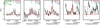Fig. 1

Best fitted model to combined Band 5 and 6 NH₂CHO data for B1-c in red and data in black. Each graph shows one line of NH₂CHO with its upper state energy level and the A_ij coefficient at the top right in red and blue, respectively. The dashed green line indicates the 3σ level. The lines above the 3σ level that were used in the fitting are indicated by a green X. The lines with upper energy levels above 1000 K and/or A_ij below 10⁻⁵ are not plotted.

Fig. 2

Same as Fig. 1 but for HN¹³CO.

3.2 Column densities

A summary of the derived column densities for B1-c and S68N is presented in Table 1. The most abundant N-bearing molecule detected towards B1-c and S68N in the Band 5 and 6 data is HNCO. The emission of this molecule is optically thick in both sources. This is also seen from a comparison of the HN¹³CO column density with the fitted HNCO column density, where the latter is under-estimated. The column densities of HNCO measured by directly fitting the spectra for HNCO are ~1.8 × 10¹⁵ cm⁻² and ~10¹⁵ cm⁻² towards B1-c and S68N, respectively. Therefore, the interstellar ratio of ¹²C/¹³C ~68 (Milam et al. 2005) was used to find HNCO column densities of 1.6 ± 0.7 × 10¹⁶ cm⁻² and ~1.2 × 10¹⁶ cm⁻² for B1-c and S68N from the HN¹³CO column densities, assuming the HN¹³CO lines are optically thin. This assumption can be investigated by searching for HNC¹⁸O lines. The Band 5 data cover HNC¹⁸O lines in B1-c. However, this molecule is not detected, and a ~3σ upper limit column density of ~4 × 10¹⁴ cm⁻² at 200 K isfound towards B1-c. This upper limit corresponds to a lower limit for the HNCO/HNC¹⁸O ratio of ≳ 40. This lower limit is smaller than the isotope ratio of ¹⁶O∕¹⁸O ~ 560 (Wilson & Rood 1994), implying that HN¹³CO emission towards B1-c could potentially be marginally optically thick. Using ¹⁶O ∕¹⁸O ~ 560 and the upper limit value for HNC¹⁸O, an upper limit for HNCO of 2.2 × 10¹⁷ cm⁻² can be found. Therefore, the value for the HNCO column density towards B1-c could potentially differ from the current value by up to an order of magnitude and hence should be taken with care. In the Band 3 data, HNCO is tentatively detected towards both sources. However, as derived above from our Band 5 and 6 data, it is optically thick, and none of its isotopologues are detected in Band 3. Therefore, we refrained from deriving the HNCO column density from the main isotopologue lines.

Unfortunately, our Band 5 and 6 frequency range covers neither CH₃CN nor its ¹⁵N or ¹³C isotopologues. The frequency range covers three rotational CH₃CN lines originating from the v₈ = 1 excited vibrational level, but they are not very constraining as they give very high upper limits on the column density at a temperature of 200 K (≲ 7 × 10¹⁸ cm⁻² and ≲ 6 × 10¹⁸ cm⁻² for B1-c and S68N, respectively). However, CH₂DCN is detected towards both sources. Given that our sources are hot corinos, in each source we used the ratio of CH₂DCN∕CH₃CN = 0.035 from the results of the PILS for IRAS 16293B (Calcutt et al. 2018) to estimate the column density of CH₃CN from our value for CH₂DCN. This is, however, only an estimate. Interestingly, CHD₂CN is also detected towards B1-c, whereas we find an upper limit for this molecule towards S68N. In Band 3, CH₃CN is clearly detected towards both sources (see Appendix C), but, given that the lines are optically thick and none of its isotopologues are detected, it is only possible to report lower limits to the actual column densities. These are ~ 10¹⁵ cm⁻² and ~ 3 × 10¹⁴ cm⁻² at a fixed temperature of 100 K (as van Gelder et al. 2020 found that Band 3 traces colder temperatures) for B1-c and S68N, respectively. These lower limits are consistent with the column densities derived for CH₃CN using the Band 6 CH₂DCN data towards both sources.

HNCO has the highest column density in both sources. CH₂DCN and CHD₂CN have the lowest column densities for S68N and B1-c, respectively. The column densities for ~ 85% of the detected and tentatively detected N-bearing species studied here are of the order of ~ 10¹⁴⁻¹⁵ cm⁻² in a 0.45′′ beam for both sources. These values are on average an order of magnitude lower than those of the O-bearing molecules studied by van Gelder et al. (2020), which is an interesting observation. Similar to what van Gelder et al. (2020) found, weaker (T_b≲ 1 K) and fewer lines are found towards the more distant S68N source compared to B1-c. On average, the column densities of the species studied in this work are ~1.5−3 times lower in S68N than in B1-c.

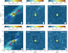Fig. 3

Moment zero maps of the lines of SO 6₇−5₆ (E_up = 47.6 K), HNCO 12_0,12−11_0,11 (E_up = 82.3 K), and NH₂CHO 13_1,13 − 12_1,12 (E_up = 91.8 K) (from left to right) for B1-c (top row) and S68N (bottom row) in the Band 6 data. The images are made by integrating over [−10, 10] km s⁻¹ with respect to V_lsr. The black contours show the continuum in levels of [15, 30, 45, 60, 75, 90, 105] σ_cont with a σ_cont of 0.2 mJy beam⁻¹ for B1-c and [30, 45, 60, 75, 90, 105, 120] σ_cont with a σ_cont of 0.09 mJy beam⁻¹ for S68N. The beam size is shown at the right-hand side of each panel. SO traces the extended outflow, while the other two molecules show compact emissions. The approximate directions of the blueshifted and redshifted emission of the outflow are shown with blue and red arrows.

3.3 Excitation temperatures

A summary of the derived excitation temperatures is presented in Table 1 for B1-c and S68N. The excitation temperatures found for the N-bearing species span a range between ~ 100 K and ~ 300 K. There is no significant difference, within the uncertainties, between the excitation temperatures for the N-bearing COMs and the O-bearing COMs found by van Gelder et al. (2020; see Sect. 4.1 for a discussion).

For most molecules, a reasonable range of upper state energy level lines is covered in our data, implying that the excitation temperatures fitted here are not biased. The only exception is NH₂CHO, where the lines included in the fit only cover upper energy levels below ~ 200 K, and thus the excitation temperature derived here is biased towards lower temperatures. Moreover, to derive the excitation temperature of HN¹³CO towards B1-c, its Band 3 data are used (in addition to the Band 6 data) as an additional constraint, eliminating very low excitation temperatures.

3.4 Column density ratios

Table 1 presents the column density ratios of the studied species with respect to CH₃OH and HNCO. The methanol column density is taken from van Gelder et al. (2020). The column density ratios of the species are not calculated with respect to H₂ because in low-mass protostars it is difficult to derive accurate values for the warm H₂ gas column density from the dust continuum or the CO column density. This is due to the fact that the dust continuum becomes optically thick at ≲100 au scales and may have contributions from a forming, colder disk (Yıldız et al. 2013; Persson et al. 2016; De Simone et al. 2020). Moreover, in low-mass sources not all CO emission comes from the region with warm gas (>100 K; Yıldız et al. 2013). Therefore, the abundances of the species considered in this work are presented with respect to CH₃OH and HNCO instead of H₂. Column density ratios with respect to methanol are given in order to compare our results with those of van Gelder et al. (2020) and other studies. The column density ratios with respect to HNCO are calculated to show whether the formation of species discussed here is linked to HNCO or routes resulting in HNCO formation (see Sect. 4.2.2).

The column density ratios for all the detected and tentatively detected molecules with respect to methanol are very similar (within a factor of two) between the two sources. This agrees with what van Gelder et al. (2020) found for most O-bearing COMs. Moreover, the column density ratios for NH₂CHO, C₂H₅CN, HNCO, and NH₂CN with respect to methanol agree, within the uncertainties, with the results of Belloche et al. (2020) for S68N observed with the PdBI. It should be noted, though, that our estimated value for CH₃CN/CH₃OH is ~ 13.5 times smaller than that derived by Belloche et al. (2020). This discrepancy could originate from the CH₃OH lines used in Belloche et al. (2020) being (marginally) optically thick, while the CH₃OH column density reported by van Gelder et al. (2020) is derived from its optically thin ¹⁸O isotopologue. It should also be noted that we find the CH₃CN column density from its deuterated isotopologues, which is another source of uncertainty. Finally, the assumed ¹⁶O/¹⁸O ratio used toderive the CH₃OH column density may differ slightly from the value assumed in van Gelder et al. (2020).

3.5 Source size and optical depth

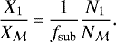
The emission from our data is not spatially resolved. Therefore, it is not obvious whether the emission is optically thin because the estimated optical depth depends on the assumed size of the emitting region. In this paper, it is assumed that the source size is the same as the ALMA Band 6 beam size of 0.45′′. A smaller source size will result in larger column densities, and hence the emission can become optically thick. This can be seen by taking the dilution factor into account. The equation $N_{1} θ_{s_{1}}^{2} / (θ_{b}^{2} + θ_{s_{1}}^{2}) = N_{2} θ_{s_{2}}^{2} / (θ_{b}^{2} + θ_{s_{2}}^{2})$ $N_{1}\theta_{\textrm{s}_{1}}^{2}/(\theta_{\textrm{b}}^{2} + \theta_{\textrm{s}_{1}}^{2})\,{=}\,N_{2}\theta_{\textrm{s}_{2}}^{2}/(\theta_{\textrm{b}}^{2} + \theta_{\textrm{s}_{2}}^{2})$ shows how the measured column density can be scaled for different source sizes (where θ_b is the beam size, θ_s is the sourcesize, and the numbers refer to the two assumed source sizes). Although the column densities would become larger for smaller source sizes that depend on the emitting region of a molecule, column density ratios will stay the same as long as the emission remains optically thin and comes from the same region.

N-bearing species identified in this work show a large range of excitation temperatures (Table 1). It is not unlikely that source sizes are different for molecules with different excitation temperatures. Here, two representative values for the excitation temperatures are considered: one for molecules that are excited at temperatures of ~ 100 K and one for molecules that are excited at temperatures of ~200 K. Therefore, one can assume two source sizes equal to two radii where temperatures are 100 K and 200 K.

Using the same method as van Gelder et al. (2020), the radius at which the temperature reaches 100 K for a spherically symmetric hot core region can be estimated from 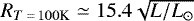$R_{T = 100 K} ≃ 15.4 \sqrt{L / L_{⊙}}$ $R_{T\,{=}\,100\textrm{K}}\simeq 15.4 \sqrt{L/L_{\odot}}\,$ au (Bisschop et al. 2007), where L is the source luminosity. The luminosities of B1-c and S68N are 6.0 L_⊙ (Karska et al. 2018) and 5.4 L_⊙ (Enoch et al. 2011), respectively. Therefore, the radii at which the temperature reaches 100 K for B1-c and S68N are about 37.7 au (0.23′′) and 35.8 au (0.16′′), respectively. When these radii are used for the line analysis, NH₂CHO remains optically thin in the Band 5 and 6 data towards B1-c even for this smaller source size. Moreover, C₂H₅CN stays optically thin for S68N at this smaller radius.

To calculate the radius at which the temperature is 200 K, we used a toy model for a spherically symmetric infalling envelope with a power law in temperature and density structure (see Appendix B). For B1-c and S68N, R_{T = 200K} is about 6.7 au (0.042′′) and 6.3 au (0.029′′), respectively. When these radii are used for the line analysis, all the molecules with high T_ex (HN¹³CO, C₂H₅CN, and CHD₂CN towards B1-c and CH₂DCN towards both sources) become optically thick in Band 5 and 6 data. Moreover, CH₃CN becomes optically thick in Band 3 for both sources, assuming its excitation temperature is similar to that of its deuterated versions (~ 200 K). It is therefore not possible to derive accurate column densities or column density ratios for such small source sizes.

It is worth noting that some deviation from spherical symmetry due to the presence of a disk can occur at < 100 au scales, and thus our simple toy model runs into limitations. Persson et al. (2016) find that the amount of gas at temperatures above 100 K in low-luminosity sources can vary by more than an order of magnitude depending on the disk size and structure, affecting optical depth. Moreover, the extremely small source sizes predicted by the simple toy model are likely unrealistic. Adopting R_{T = 100K} as the source size for both sources, all molecules in Band 5 and 6 remain optically thin and CH₃CN remains marginally optically thick (τ > 0.1) in Band 3 for both sources as expected (see Sect. 3.2). For this reason, assuming a source size of 0.45′′ in the rest of this paper does not change our results.

4 Discussion

4.1 Excitation versus desorption temperatures

Figure 4 presents a comparison between excitation temperatures of the O-bearing species studied by van Gelder et al. (2020) and the N-bearing species studied in this work towards B1-c and S68N. This figure shows that there is no significant difference in T_ex between the O-bearing and N-bearing species; the mean and the scatter of T_ex are very similar. Assuming that the excitation temperature is close to the kinetic temperature of the region in which a molecule resides, Fig. 4 suggests that N-bearing species trace a range of temperatures from ~ 100 K to ~ 300 K. We note that at the densities considered here some molecules may be sub-thermally excited, and hence the T_ex found in this work may be a lower limit to the kinetic temperature (Jørgensen et al. 2016). Bisschop et al. (2007) also found that there isno difference between the excitation temperatures of N-bearing and O-bearing species in seven high-mass protostars, which is consistent with what is found here.

Each molecule can desorb at a significantly different temperature according to its binding energy, ice, and grain environment (Cuppen et al. 2017), so molecules come off the ice roughly at their respective snow lines depending on their sublimation temperatures. Therefore, one would expect differences in the excitation temperatures of molecules. The idea of an onion-like temperaturestructure around low-mass protostars was discussed in Jørgensen et al. (2018), in which O-bearing molecules are divided into two categories (see also Manigand et al. 2020): one that includes molecules associated with temperatures of 100–150 K and another that includes molecules associated with temperatures of 250–300 K. Figure 4 shows that C₂H₅CN towards B1-c falls under the hottest category (>250 K). In addition, three of the N-bearing molecules studied here (HN¹³CO, CH₂DCN, and CHD₂CN) seem to trace the gas with temperatures around ~200 K in B1-c.

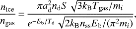
The potential relation between the excitation and sublimation temperatures of molecules can be further explored by comparing our results with the sublimation temperatures found from the gas-grain balance model (Hasegawa et al. 1992) and the binding energies of each molecule in the solid state. In this model, the number density of the solid to the gas phase of species i is given by $\frac{n_{ice}}{n_{gas}} = \frac{π a_{d}^{2} n_{d} S \sqrt{3 k_{B} T_{gas} / m_{i}}}{e^{- E_{b} / T_{d}} \sqrt{2 k_{B} n_{ss} E_{b} / (π^{2} m_{i})}},$ $\begin{equation*} \frac{n_{\textrm{ice}}}{n_{\textrm{gas}}}\,{=}\,\frac{\pi a_{\textrm{d}}^{2} n_{\textrm{d}} S \sqrt{3k_{\textrm{B}}T_{\textrm{gas}}/m_{i}}}{e^{-E_{\textrm{b}}/T_{\textrm{d}}} \sqrt{2 k_{\textrm{B}} n_{\textrm{ss}} E_{\textrm{b}}/(\pi^{2}m_{i})}},\end{equation*}$ (1)

where a_d is the dust grain size (assumed to be 0.1 μm), n_d = 10⁻¹² × n_H is the dust number density (with n_H the hydrogen number density, assumed to be 10⁷ cm⁻³), S is the sticking coefficient (assumed to be 1), n_ss is the number of binding sites per surface area (taken as 8 × 10¹⁴ cm⁻²), E_b is the binding energy of species i in units of kelvin, m_i is the mass of species i, and T_gas and T_d are the gas and dust temperatures, respectively. Assuming that the environment is sufficiently dense, the gas would be thermally coupled with the dust and T_d would be equal to T_gas. The sublimation temperatureof species i is the temperature for which the ice and the gas are in balance for that molecule. In other words, n_ice ∕n_gas = 1.

Therefore, using Eq. (1) and the binding energies for most molecules from Penteado et al. (2017; the binding energy for (CH₂OH)₂ is taken from Garrod 2013), the desorption temperatures of O-bearing and N-bearing species can be calculated. The grey points in Fig. 4 represent these values. It can be safely assumed that the desorption temperatures for the isotopologues will barely differ from that of the main isotopologue. However, binding energies differ for different molecule interactions in a mixed ice or on different grain surfaces (e.g. Tielens et al. 1991; Collings et al. 2004; Ferrero et al. 2020), and hence in principle desorption temperatures may vary (typically by several tens of kelvin). The values adopted here are mostly for pure ices; if these COMs are mixed in ice layers consisting predominantly of H₂O or CH₃OH, values close to their desorption temperatures (~100 K) are expected.

Figure 4 shows that there is no significant difference between the sublimation temperatures of O-bearing and N-bearing species. This is consistent with what is seen for the excitation temperatures, but with an offset between sublimation temperatures and excitation temperatures for most molecules (except for (CH₂OH)₂). Specifically, the excitation temperatures are typically higher than the sublimation temperatures for all molecules by a factor of ~ 2−4, except for (CH₂OH)₂ where these two values are very similar. This can be interpreted as the excitation temperatures reflecting an average temperatureof the region around the protostar, where it is hotter than the sublimation temperature of each molecule. Using the toy model for a spherically symmetric infalling envelope with power law structure in temperature and density (see Appendix B.4), the mass-weighted average temperature can be calculated as 1.36 T_sub. Therefore, ifthe excitation temperature is measuring an average temperature, it is expected to be larger than the sublimation temperaturefor each molecule. We note that the factor 1.36 is not large enough to explain the difference seen in Fig. 4. However, this is only using a simple toy model: Developing a more complete model that takes small-scale structures such as disks into account can improve our understanding of the difference between sublimation temperatures and excitation temperatures.

The sublimation temperatures for all species in Fig. 4 (except for (CH₂OH)₂) are between ~55 and ~125 K. While the sublimation temperatures of O-bearing and N-bearing groups of species do not differ significantly, these values for some molecules (i.e. CH₃OCH₃, CH₃CHO, and HNCO) are lower than the rest, and others (i.e. C₂H₅CN and (CH₂OH)₂) are higher. Such trends are reflected in the excitation temperatures for some of the molecules with small error bars. For example, CH₃OCH₃ shows very low excitation temperatures in both sources, which agrees with its low sublimation temperature. This may be good evidence for the formation of this molecule in the ice and its desorption at its snow line. On the other hand, a molecule such as CH₃CHO shows a larger excitation temperature compared to the other species, in contradiction with its low sublimation temperature. This could be evidence for other mechanisms (e.g. gas-phase formation pathways or source structures) potentially playing a role in the formation (Garrod et al. 2008; Tideswell et al. 2010; Vazart et al. 2020) and emission of these species. However, given the large error bars on most of the excitation temperatures shown in Fig. 4, all these arguments should be taken with care.

Using Herschel-HIFI data, Crockett et al. (2015) find that N-bearing species, C₂H₅CN, NH₂CHO, and CH₃CN, trace hotter gas (~ 250 K) compared with the oxygen-bearing species, CH₃OH, CH₃OCH₃, C₂H₅OH, and CH₃OCHO, (~ 100 K), in the OrionKleinmann–Low nebula (see Fig. 5). They argue that this could indicate either that N-bearing COMs require higher dust temperatures to desorb from the ice or that more N-bearing molecules are formed through high temperature gas-phase chemistry, reflecting the two possible COM formation scenarios: colder solid-state chemistry and warmer gas-phase chemistry.

Alternatively, at such high temperatures Crockett et al. (2015) could be seeing the carbon grain sublimation into the gas phase that leads to the formation ofCH₃CN, an idea putforward by van ’t Hoff et al. (2020a). They propose the formation of N-rich COMs inside a ‘soot line’ at 300 K through carbon grain sublimation and suggest that an excess of hydrocarbons and nitriles withexcitation temperatures higher than those of O-bearing species can be a signature of this phenomenon. This process implies that such molecules could be formed through top-down chemistry (from the destruction of larger species) rather than bottom-up chemistry in the solid state or gas phase. van ’t Hoff et al. (2020a) assume that no molecules with oxygen atoms are formed through carbon grain sublimation inside of the soot line at ~ 300 K as all the oxygen is locked up in H₂O, CO, and CO₂. Thus, the only two molecules in this work that can be signatures for carbon grain sublimation are C₂H₅CN and CH₃CN. The toy model for a spherically symmetric infalling envelope explained in Appendix B.4 predicts the ~ 300 K radius to be significantly smaller than the spatial resolution of our data. Therefore, the fact that carbon grain sublimation is not seen for C₂H₅CN and CH₃CN in B1-c or S68N might be due to this effect being concealed at the present spatial resolution.

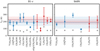Fig. 4

Excitation temperatures for N-bearing species discussed in this work (red) and O-bearing species discussed in van Gelder et al. (2020) (blue) for B1-c and S68N. Only the species with derived T_ex are plotted. The solid red and blue lines show the average values for the red and blue data points, respectively. The shaded red and blue areas show the standard deviation of the data points. The grey points show the sublimation temperatures of the corresponding molecules found by the gas-grain balance model (Hasegawa et al. 1992) and the respective binding energies of each molecule (Penteado et al. 2017; Garrod 2013).

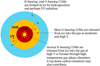Fig. 5

Cartoon of the temperature structure of protostellar envelopes showing where O-bearing and N-bearing species are most likely to be found in the gas. This is based on the findings of Crockett et al. (2015) for massive protostars, who showedthat higher excitation temperatures for N-bearing COMs are found towards several high-mass protostars, and van ’t Hoff et al. (2020a), who proposed a top-down carbon chemistry for nitriles. It is not yet clear whether this structure also applies to low-mass protostars.

4.2 Comparison of abundances in different sources

In this section, the column density ratios of B1-c and S68N are compared with other sources. In most studies, column density ratios are interpreted as abundances. Therefore, this section also assumes no difference between column density ratios and abundances. The validity of this assumption is further discussed in Sect. 4.3.

4.2.1 Dependence on luminosity

Higher luminosity implies a higher temperature, where chemical reactions can take place more efficiently thereby affecting the production rate of molecules and possibly changing their abundances. In addition, a source with a higher luminosity has more UV radiation, and hence the UV processing on the grains can alter the gas-phase abundances of species, for example through (non-)dissociative photo-desorption but also following UV-induced photochemistry in the ice (Öberg et al. 2009b; Bertin et al. 2013). Therefore, a relation between the luminosity and the abundance of a species with respect to methanol may be present. This is especially important for species with higher desorption temperatures (e.g. NH₂CHO; see Sect. 4.1) that may stay mostly in the ice in sources with lower luminosities.

Figure 6 shows the abundances of NH₂CHO and HNCO with respect to methanol for our sources and other low- and high-mass protostars against the source luminosity (see the caption of Fig. 6 for the full list of sources and reference papers). There is no significant relation between abundances and source luminosity. The same conclusion holds true for the rest of the N-bearing species, which is consistent with the results of van Gelder et al. (2020) for the O-bearing COMs. Moreover, our results are consistent with what Belloche et al. (2020) find for protostellar sources observed by the PdBI. Nevertheless, Fig. 6 shows that NH₂CHO/CH₃OH ranges from ~0.01% to ~0.1% (discussed further in Sect. 4.2.2), whereas van Gelder et al. (2020) find that for most O-bearing molecules the column density ratios with respect to methanol are within a factor of a few for various sources. Given that in all these sources the methanol column density is derived from one of its optically thin isotopologues, the difference seen here cannot be due to issues with optical depth.

4.2.2 Abundances with respect to CH₃OH and HNCO

We compared our abundances to values obtained for other low-mass and high-mass sources that have been studied by ALMA. The low-mass sources are IRAS 16293A (Coutens et al. 2016; Ligterink et al. 2017; Calcutt et al. 2018; Manigand et al. 2020), IRAS 16293B (Coutens et al. 2016; Ligterink et al. 2017; Jørgensen et al. 2018; Calcutt et al. 2018; Coutens et al. 2018), HH 212 (Lee et al. 2019), and NGC 1333 IRAS 4A2 (López-Sepulcre et al. 2017). The high-mass sources are AFGL 4176 (Bøgelund et al. 2019a) and NGC 6334 MM1, MM2, and MM3 (Bøgelund et al. 2019b).

Figure 7 shows this comparison for the ratio of the column densities to methanol. At a glance, we can see that these values are generally lower than those of O-bearing species (Fig. 7 in van Gelder et al. 2020), typically by an order of magnitude. Moreover, there is a larger variation (up to an order of magnitude) between the different sources for N-bearing molecules than for O-bearing ones (by a factor of a few).

When comparing the column density ratios of the N-bearing species shown in Fig. 7 among different sources, one can see that some molecules show similar abundance ratios. Most notably, C₂H₅CN is comparable in the low-mass sources and with the high-mass AFGL 4176 (within a factor of ~ 5).

A larger scatter (around an order of magnitude) is seen for NH₂CHO between all sources (see also Fig. 6). Three categories seem to be present. First, two of the high-mass sources (NGC6334 MM1 and MM2) seem to agree with three of the low-mass sources (B1-c, S68N, and IRAS 16293A). Second, the high-mass source, AFGL 4176, is similar to the two other low-mass sources, IRAS 16293B and HH212.Third, the high-mass source NGC 6334 MM3 does not show a detection of this COM. Manigand et al. (2020) explain the low abundance ratio of formamide in IRAS 16293A compared with IRAS 16293B by the fact that the offset position used to extract the spectrum for the former seems to be missing the hottest gas and thus most of the emission from this molecule, while this is not the case for the latter. Moreover, in contrast with our results, they find that formamide belongs to a group of species with a high excitation temperature. Another possible explanation for the variation in formamide abundance ratios with respect to methanol across various sources is the fact that there are multiple ways to form formamide in the solid state (Rimola et al. 2018; Haupa et al. 2019; Dulieu et al. 2019; Martín-Doménech et al. 2020) and gas phase (Barone et al. 2015; Codella et al. 2017). Therefore, the amount of this COM formed in the gas or ice could depend on local conditions, such as the presence of a disk, its temperature structure (Jørgensen et al. 2002; Schöier et al. 2002; Crimier et al. 2010), or its exposure to UV (López-Sepulcre et al. 2019).

HNCO and its isotopologues show some scatter in their distributions with respect to methanol. B1-c (0.9 ± 0.5%), S68N (0.9 ± 0.4%), and the high-mass source AFGL 4176 (1.1 ± 0.3%) seem to have a more similar distribution of HNCO with respect to methanol, while the IRAS 16293 sources show a lower abundance ratio (0.17 ± 0.07% and 0.37 ± 0.13% for IRAS 16293A and B, respectively).

Figure 8 shows the abundance ratios of the molecules studied in this work with respect to HNCO. The scatter that was seen in Fig. 7 seems to be less pronounced for most molecules. Among them, DNCO has a more uniform distribution between sources, as expected for a molecule formed directly via the deuteration of HNCO (Noble et al. 2015). Another molecule that shows a much more uniform distribution among sources is CHD₂CN. Ligterink et al. (2020) studied amide molecules towards 12 positions in the high-mass star-forming region NGC 6334I. Their values of NH₂CHO/HNCO measured from the ¹³C isotopologues of these two species span a range between ~10% and ~100%. This range is ~1−2 orders of magnitude higher than what is found in this work towards B1-c and S68N, and more similar to IRAS 16293B (Fig. 8).

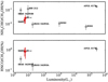Fig. 6

Abundance ratio of NH₂CHO and HNCO with respect to CH₃OH against source luminosity. Red points show the results for the sources considered in this work. The grey points indicate other low- and high-mass sources. These sources are IRAS 16293A (Ligterink et al. 2017; Manigand et al. 2020), IRAS 16293B (Coutens et al. 2016; Ligterink et al. 2017; Jørgensen et al. 2018), HH 212 (Lee et al. 2019), AFGL 4176 (Bøgelund et al. 2019a), and NGC6334 MM1 and MM2 (Bøgelund et al. 2019b).

4.2.3 Deuteration fraction

B1-c and S68N are known to have a high deuteration fraction, as confirmed for methanol by van Gelder et al. (2020) from CH₂DOH. Jørgensen et al. (2018) found that less complex molecules have similar D/H ratios. For example, the D/H ratios for HNCO (~ 1%; Coutens et al. 2016) and CH₃OH (2%; Jørgensen et al. 2018) in IRAS 16293B are comparable. Therefore, we similarly compared D/H for these two molecules in B1-c and S68N. The deuteration fraction found from this work for B1-c and S68N from the DNCO/HNCO ratio are 1.8 ± 0.8% and < 0.6%. The value for B1-c is in agreement with the 2.7 ± 0.9% methanol value reported in van Gelder et al. (2020), whereas the upper limit found for S68N is somewhat lower than the 1.4 ± 0.6% methanol value reported in the same study.

The D/H ratio can provide a clue as to the temperature history of the environment in which B1-c is forming. This can also be seen in Fig. 8, where DNCO, CHD₂CN, and CH₂DCN have abundance ratios with respect to HNCO that agree, within the uncertainties, between the low-mass sources. These sources are from different star-forming regions and yet show similar abundance ratios, pointing to the fact that there is a universal mechanism for increasing the D/H ratio prior to star formation in cold environments.

For CH₂DCN/CHD₂CN, a column density ratio of ~2 is found towards B1-c, which is lower than that found for IRAS 16293A (~ 16) and IRAS 16293B (~7) by Calcutt et al. (2018). On the other hand, Taquet et al. (2019) find CH₂DOH/CHD₂OH ~ 1 and ~2 for NGC 1333-IRAS2A and NGC 1333-IRAS4A, values that are more similar to our ratio for the deuterated versions of methyl cyanide. In general, these similarities and differences are interesting, but, given the small sample of hot corinos with a similar analysis at hand, we did not investigate this further.

Fig. 7

Column densities of the N-bearing molecules with respect to methanol for sources observed by ALMA. Column densities of methanol for B1-c and S68N are taken from van Gelder et al. (2020). Shown are IRAS 16293A (Coutens et al. 2016; Ligterink et al. 2017; Calcutt et al. 2018; Manigand et al. 2020), IRAS 16293B (Coutens et al. 2016, 2018; Ligterink et al. 2017; Jørgensen et al. 2018; Calcutt et al. 2018), HH 212 (Lee et al. 2019), AFGL 4176 (Bøgelund et al. 2019a), and NGC 6334 MM1, MM2, and MM3 (Bøgelund et al. 2019b).

Fig. 8

Column densities of N-bearing species with respect to HNCO as derived from HN¹³ CO. Shown are IRAS 16293A (Coutens et al. 2016; Ligterink et al. 2017; Calcutt et al. 2018; Manigand et al. 2020), IRAS 16293B (Coutens et al. 2016, 2018; Ligterink et al. 2017; Calcutt et al. 2018), NGC 1333 IRAS 4A2 (López-Sepulcre et al. 2017), and AFGL 4176 (Bøgelund et al. 2019a).

4.2.4 Comparison with ices

B1-c is an ice-rich source, but so far CH₃OH is the only COM that has been identified along the line of sight towards the neighbouring B1-b source with Spitzer (Boogert et al. 2008). Ices have also been detected towards S68N (e.g. Anderson et al. 2013), but they have not yet been analysed in detail. However, OCN⁻, a direct derivative of HNCO (van Broekhuizen et al. 2004; Fedoseev et al. 2016), is observed towards many low- and high-mass protostars (van Broekhuizen et al. 2005; Öberg et al. 2011). Öberg et al. (2011) find that, for the low-mass sources in their study, the median values for OCN⁻ and CH₃OH ice abundances with respect to water ice are ${0.4}_{0.3}^{0.4} %$ $0.4^{0.4}_{0.3}\%$ and $7_{5}^{12}$ $7^{12}_{5}$ %, respectively. This gives an abundance ratio of OCN⁻ with respectto CH₃OH of $~ 6_{2.5}^{8} %$ ${\sim} 6_{2.5}^{8}\%$ . This abundance ratio shows a considerable spread from source to source. Our gas-phase abundance ratios of HNCO to CH₃OH are ~0.9 ± 0.5% and ~0.9 ± 0.4% for B1-c and S68N, respectively (Table 1). These values are ~ 6 times lower than the median ice ratio but close to its lower limit. This comparison assumes that all OCN⁻ comes off the grains as HNCO upon ice sublimation, but some of it may be converted into other species, such as more refractory salts (Schutte & Khanna 2003; Boogert et al. 2008). This is a reasonable assumption given that N-bearing salts are found to be abundant in comet 67P (Altwegg et al. 2020).

In addition, there are also upper limit estimates for HNCO ice itself, but mostly for high-mass protostars. Taking the upper limit of 0.7% for HNCO/H₂O ice from van Broekhuizen et al. (2004, 2005) and dividing it by the median of the CH₃OH/H₂O ice ratio in high-mass protostars ( $8_{8}^{16} %$ $8^{16}_{8}\%$ ) from Öberg et al. (2011) gives an upper limit estimate of 9% for the HNCO/CH₃OH ice ratio. Again, this is higher than our observed ratios in low-mass hot corinos.

These differences are interesting, but without the direct observation of the species studied here in ices for the same sources it is not possible to investigate this further. The column density ratios discussed in this section need to be studied in a larger sample of protostars to make progress in this field. More robust conclusions will become possible with the launch of JWST and the direct observation of these molecules in ices. In addition, progress in recording the solid state features of several species will make this comparison more plausible in the near future (Boudin et al. 1998; Terwisscha van Scheltinga et al. 2018; Gerakines & Hudson 2020).

4.3 Effect of emitting areas of molecules on abundance ratios

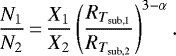
As the emission from our data is not spatially resolved, variations from source to source or molecule to molecule could be explained by different emitting regions that are possibly related to different binding energies. Using the spherically symmetric infalling envelope toy model (see Appendix B), we can find a relation between the ratio of column densities of two molecules inthe same beam with the ratio of their corresponding sublimation temperatures. This is given as 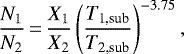$\frac{N_{1}}{N_{2}} = \frac{X_{1}}{X_{2}} {(\frac{T_{1, sub}}{T_{2, sub}})}^{- 3.75},$ $\begin{equation*} \frac{N_{1}}{N_{2}}\,{=}\,\frac{X_{1}}{X_{2}} \left(\frac{T_{\textrm{1,sub}}}{T_{\textrm{2,sub}}}\right)^{-3.75},\end{equation*}$ (2)

where X is the abundance of a molecule in gas phase with respect to molecular hydrogen, N is the column density, and T_sub is the sublimation temperature, with subscripts 1 and 2 indicating the two species. Equation (2) shows that the column density ratios depend not only on the abundance ratios but also on the ratio of sublimation temperatures. This is because the difference in the sublimation temperature results in a difference in the emitting volume.

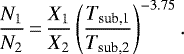
Figure 4 shows that a typical O-bearing or N-bearing molecule, $M$ $\mathcal{M}$ , comes off the grains at a temperature of ~100 K. Hence, one can rewrite Eq. (2) for species 1 as 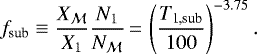$f_{sub} \equiv \frac{X_{M}}{X_{1}} \frac{N_{1}}{N_{M}} = {(\frac{T_{1, sub}}{100})}^{- 3.75} .$ $\begin{equation*} f_{\textrm{sub}} \equiv \frac{X_{\mathcal{M}}}{X_{1}} \frac{N_{1}}{N_{\mathcal{M}}}\,{=}\,\left(\frac{T_{\textrm{1,sub}}}{100}\right)^{-3.75}.\end{equation*}$ (3)

This can be rewritten as $\frac{X_{1}}{X_{M}} = \frac{1}{f_{sub}} \frac{N_{1}}{N_{M}} .$ $\begin{equation*} \frac{X_{1}}{X_{\mathcal{M}}}\,{=}\,\frac{1}{f_{\textrm{sub}}} \frac{N_{1}}{N_{\mathcal{M}}}.\end{equation*}$ (4)

The column density ratios discussed in this work with respect to methanol, which has a T_sub of ~ 100 K, are thus the abundance ratios with respect to methanol times a factor (f_sub). The abundance of a molecule is a local quantity that is sensitive to the emitting area, but column density is an integrated quantity within a given beam. In other words, using the expression ‘abundance’ to refer to a column density ratio is only accurate if the emitting areas are similar.

Figure 9 shows f_sub as defined in Eq. (3) against the sublimation temperature for a molecule. This figure shows that, for species with desorption temperatures between 55 K and 125 K (see the grey points in Fig. 4), one would need to multiply the column density ratios of the species with respect to methanol by a factor of between 0.1 and 2 to get the respective abundance ratios. This factor becomes much larger as the sublimation temperature increases. For instance, (CH₂OH)₂ has a sublimation temperature of ~200 K, and hence the factor becomes ~14 for this molecule. However, this factor is not applied here because of the simplicity of our model. In reality, one needs to build a model that takes small-scale structures such as disks into account (Harsono et al. 2015; Persson et al. 2016), as discovered by other studies of Class 0 objects (Tobin et al. 2012; Murillo et al. 2013; Martín-Doménech et al. 2019; Maret et al. 2020). This is important because the temperature profile in an envelope of a Class 0 object does not correspond to the temperature profile in the inner regions of the disk (Murillo et al. 2018; van ’t Hoff et al. 2020c). Moreover, the opacity of the dust continuum emission can also become relevant at ≲ 50 au scales (De Simone et al. 2020).

In conclusion, some of the variations seen in abundances between various molecules and between different sources maybe related to different emitting regions originating from different binding energies rather than from chemistry.

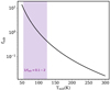Fig. 9

Correction factor, f_sub, introduced in Eq. (4) due to different emitting areas arising from the sublimation temperature. The shaded area shows where most of the species considered in this work fall on this graph (sublimation temperatures between 55 K and 125 K).The abundance ratios of these species with respect to methanol are found by multiplying their column density ratios with respect to methanol by a factor of between 0.1 and 2.

5 Conclusions

In this work, we derived the column densities and excitation temperatures of N-bearing species in two Class 0 objects, B1-c and S68N, using the Band 6, Band 5, and Band 3 of ALMA. The main conclusions are listed below.

Four N-bearing molecules and their isotopologues are identified towards B1-c and S68N with ALMA. These species are HNCO, HN¹³CO, DNCO, C₂H₅CN, NH₂CHO, CH₃CN, CH₂DCN, and CHD₂CN. None of these species are spatially resolved, but they are located within 200 au of the central protostar.
N-bearing and O-bearing species show a similar scatter in their excitation temperatures (~100–300 K), and the average excitation temperature of N-bearing species is roughly the same as the average for the O-bearing species studied by van Gelder et al. (2020) for B1-c and S68N.
The excitation temperatures for the N-bearing and O-bearing species are larger than the sublimation temperatures of each molecule, which span a range between ~55 and ~125 K. This can be interpreted as the excitation temperature measuring a mass-weighted average temperature of the region that is hotter than the sublimation temperature of the detected molecule.
The abundances of the N-bearing species with respect to methanol and HNCO are very similar for the two sources studied in this work. Their abundances with respect to methanol are lower than those of the O-bearing species by an order of magnitude.
Overall, N-bearing species show more uniform abundance ratios with respect to HNCO than relative to methanol between low- and high-mass sources.
CH₂DCN, CHD₂CN, and DNCO show similar abundance ratios with respect to HNCO between different low-mass sources, suggesting a universal mechanism for increasing the D/H in cold regions prior to the star formation process.
The NH₂CHO/CH₃OH varies within an order of magnitude between different sources. This can be due either to the different formation pathways suggested for formamide in the solid state or the high sublimation temperature of formamide and the different local temperatures where formamide is detected.
Variation in abundance ratios between various molecules and sources could be due to the different emitting areas related to the binding energies of the species in spatially unresolved emission.

We emphasise that the sample of COM-rich low-mass protostars that have been subjected to such analyses is still very small. Therefore, reaching robust conclusions on the chemistry of the species discussed here is difficult. An increase in the size of this sample by an order of magnitude will enhance our understanding considerably. Moreover, a broader frequency coverage can help to determine more accurate excitation temperatures and identify other molecular species. Therefore, more ALMA and NOEMA observations of COM-rich Class 0/I objects are necessary for moving this field forward. Moreover, JWST data of the sources discussed here can give a direct comparison between the ice abundances and the gas abundances found in this work. The conclusions presented here can act as a guideline for this future work.

Acknowledgements

We thank the Allegro Team at Leiden Observatory, especially Aida Ahmadi for her invaluable help in reducing the Band 5 data for B1-c. We also thank the referee for a constructive report. This paper makes use of the following ALMA data: ADS/JAO.ALMA# 2017.1.01174.S and ADS/JAO.ALMA# 2017.1.01371.S. ALMA is a partnership of ESO (representing its member states), NSF (USA) and NINS (Japan), together with NRC (Canada), MOST and ASIAA (Taiwan), and KASI (Republic of Korea), in cooperation with the Republic of Chile. The Joint ALMA Observatory is operated by ESO, AUI/NRAO and NAOJ. Astrochemistry in Leiden is supported by the NetherlandsResearch School for Astronomy (NOVA). M.L.G. acknowledges support from the Dutch Research Council (NWO) with project number NWO TOP-1 614.001.751. B.T. acknowledges support from the Dutch Astrochemistry Network II with project number 614.001.751, financed by the Netherlands Organisation for Scientific Research (NWO). M.L.R.H. acknowledges support from the Michigan Society of Fellows. A.C.G. has received funding from the European Research Council under the European Union’s Horizon 2020 research and innovation programme (grant agreement No. 743029). H.B. acknowledges support from the European Research Council under the Horizon 2020 Framework Program via the ERC Consolidator Grant CSF-648505. H.B. also acknowledges support from the Deutsche Forschungsgemeinschaft in the Collaborative Research Center (SFB 881) “The Milky Way System” (subproject B1).

Appendix A Spectroscopic data

The spectroscopic data for HNCO are taken from the CDMS (Müller et al. 2001, 2005), which is based on the work by Kukolich et al. (1971), Hocking et al. (1975), Niedenhoff et al. (1995), and Lapinov et al. (2007). DNCO and HN¹³CO data are based on Hocking et al. (1975) and are taken from the JPL database (Pickett et al. 1998).

The line list for C₂H₅CN is taken from the CDMS. The molecule entries are based on the work by Pearson et al. (1994), Fukuyama et al. (1996), and Brauer et al. (2009). A vibrational factor of 1.8316 is used at 200 K (Heise et al. 1981).

The line list for NH₂CHO is taken from the JPL database. The methods used to analyse the experimental measurements are in Kirchhoff (1972). The measurements are taken from Kurland & Wilson (1957), Costain & Dowling (1960), Kukolich & Nelson (1971), Johnson et al. (1972), and Kirchhoff & Johnson (1973). An upper limit of 1.5 for the vibrational correction factor of NH₂CHO is used at 300 K.

The spectroscopic data used for CH₃CN are taken from the CDMS entry (Bocquet et al. 1988; Koivusaari et al. 1992; Tolonen et al. 1993; Anttila et al. 1993; Gadhi et al. 1995; Šimečková et al. 2004; Cazzoli & Puzzarini 2006; Müller et al. 2009, 2015). The line lists of CH₂DCN and CHD₂CN are taken from the CDMS (Nguyen et al. 2013). CH₂DCN has additional data from Le Guennec et al. (1992) and Müller et al. (2009). CHD₂CN has additional data from Halonen & Mills (1978). The vibration factor for CH₃CN is lower than 1.1 up to a temperature of 180 K (Müller et al. 2015) and is thus negligible in this work. It is assumed that the difference between the vibrational factors for the main molecule and its isotopologues are small at the excitation temperatures found in this work.

The spectroscopic data for CH₃NCO are taken from the CDMS (Koput 1986; Cernicharo et al. 2016). The partition function takes vibrational states into account up to 580 K. The line list for NH₂CN is taken from the JPL database (Read et al. 1986). The spectroscopic data for HOCH₂CN are taken from the CDMS (Margulès et al. 2017). The line list for CH₃NH₂ is taken from the JPL database (Ilyushin et al. 2005; Kréglewski & Wlodarczak 1992; Krȩglewski et al. 1992; Ohashi et al. 1987; Takagi & Kojima 1971; Nishikawa 1957; Lide 1954; Shimoda et al. 1954; Lide 1957).

Appendix B Toy model for a spherically symmetric envelope

B.1 Physical model

A toy model for a spherically symmetric infalling envelope can be developed by assuming a power law structure in density and temperature. The number density of hydrogen is assumed to be 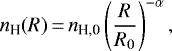$n_{H} (R) = n_{H, 0} {(\frac{R}{R_{0}})}^{- α},$ $\begin{equation*} n_{\textrm{H}}(R)\,{=}\,n_{\textrm{H,0}} \left(\frac{R}{R_{0}}\right)^{-\alpha},\end{equation*}$ (B.1)

where α is 3/2 for a free-falling envelope, R is the radius, and n_H,0 is the number density of hydrogen at radius R₀. Moreover, assuming that the envelope is passively heated by the central protostar, the temperature profile can be written as $T (R) = T_{0} {(\frac{R}{R_{0}})}^{- β},$ $\begin{equation*} T(R)\,{=}\,T_{0} \left(\frac{R}{R_{0}}\right)^{-\beta},\end{equation*}$ (B.2)

where β ≃ 2∕5 (at R ≳ 10 au) from radiative transfer calculations (Adams & Shu 1985) and T₀ is the temperature at R₀ and is proportional to $L_{bol}^{1 / 5}$ $L_{\textrm{bol}}^{1/5}$ , where L_bol is the bolometric luminosity of the source.

In this model, we assume that a constant amount of material crosses the snow line and sublimates into the gas phase without further gas-phase reactions. Therefore, each COM comes off the ice at its sublimation temperature, T_sub, corresponding to a sublimation radius of $R_{T_{sub}}$ $R_{T_{\textrm{sub}}}$ . This radius is found by rearranging Eq. (B.2): $R (T_{sub}) = R_{0} {(\frac{T_{sub}}{T_{0}})}^{- 1 / β} .$ $\begin{equation*} R(T_{\textrm{sub}})\,{=}\,R_{0} \left(\frac{T_{\textrm{sub}}}{T_{0}}\right)^{-1/\beta}.\end{equation*}$ (B.3)

B.2 Scaling of COM emission with luminosity

Assuming the emission is optically thin, the total number of a specific COM in the gas phase that comes off the ice at temperatures above its sublimation temperature is proportional to the line flux. The total number of a molecule of a specific COM, $N_{i}$ $\mathcal{N}_i$ , is given by: $\begin{array}{l} N_{i} & = \int_{0}^{R_{T_{sub}}} 4 π X_{i} n_{H} (R) R^{2} d R \\ = 4 π X_{i} \int_{0}^{R_{T_{sub}}} n_{H, 0} {(\frac{R}{R_{0}})}^{- α} R^{2} d R \\ = \frac{4 π}{3 - α} X_{i} n_{H, 0} R_{0}^{α} R_{T_{sub}}^{3 - α}, \end{array}$ $\begin{align*} \mathcal{N}_{i} &\,{=}\,\int_{0}^{R_{T_{\textrm{sub}}}} 4 \pi X_{i} n_{\textrm{H}}(R) R^{2}\,\textrm{d}R \\ &\,{=}\,4\pi X_{i} \int_{0}^{R_{T_{\textrm{sub}}}} n_{\textrm{H,0}} \left(\frac{R}{R_{0}}\right)^{-\alpha} R^{2}\,\textrm{d}R \\ &\,{=}\,\frac{4\pi}{3-\alpha} X_{i} n_{\textrm{H,0}} R_{0}^{\alpha} R_{T_{\textrm{sub}}}^{3-\alpha},\end{align*}$

where X_i is the abundance of species i with respect to hydrogen atoms.

Dropping the factors that do not depend on the source properties, Eqs. (B.3) and (B.6) yield $N_{i} \propto n_{H, 0} R_{T_{sub}}^{3 - α} \propto n_{H, 0} T_{0}^{(3 - α) / β} \propto n_{H, 0} L_{bol}^{(3 - α) / (5 β)},$ $\begin{equation*} \mathcal{N}_{i} \propto n_{\textrm{H,0}} R_{T_{\textrm{sub}}}^{3- \alpha} \propto n_{\textrm{H,0}} T_{0}^{(3-\alpha)/\beta} \propto n_{\textrm{H,0}} L_{\textrm{bol}}^{(3 - \alpha)/(5\beta)},\end{equation*}$ (B.7)

and assuming α = 3∕2 and β = 2∕5 gives $N_{i} \propto n_{H, 0} L_{bol}^{3 / 4} .$ $\begin{equation*} \mathcal{N}_{i} \propto n_{\textrm{H,0}} L_{\textrm{bol}}^{3/4}. \end{equation*}$ (B.8)

Therefore, the toy model predicts that the total number of molecules depends on the density of the envelope at a reference radius, R₀, and on the luminosity of the source.

B.3 COM emission as a function of T_sub

The measured column density of a molecule depends on the assumed source size. If the emission is spatially unresolved and optically thin, one generally assumes a fixed source size for the different species. Hence, the ratio of the measured column densities of two species, 1 and 2, does not depend on the assumed source size. Moreover, the ratio of the measured column densities, assuming the same emitting region, is the same as the ratio of the number of the two molecules in the gas phase. Therefore, the ratio of column densities as found in Sect. 3.2 (N₁ ∕N₂) is the sameas the ratio of the total number of molecules for two COMs ( $N_{1} / N_{2}$ $\mathcal{N}_{1}/\mathcal{N}_{2}$ ). For the rest of this section, N₁∕N₂ and $N_{1} / N_{2}$ $\mathcal{N}_{1}/\mathcal{N}_{2}$ are the same.

From Eq. (B.6), this ratio is given by $\frac{N_{1}}{N_{2}} = \frac{X_{1}}{X_{2}} {(\frac{R_{T_{sub, 1}}}{R_{T_{sub, 2}}})}^{3 - α} .$ $\begin{equation*} \frac{N_{1}}{N_{2}}\,{=}\,\frac{X_{1}}{X_{2}} \left(\frac{R_{T_{\textrm{sub,1}}}}{R_{T_{\textrm{sub,2}}}}\right)^{3-\alpha}. \end{equation*}$ (B.9)

Using Eq. (B.3) and assuming α = 3∕2 and β = 2∕5, this becomes $\frac{N_{1}}{N_{2}} = \frac{X_{1}}{X_{2}} {(\frac{T_{sub, 1}}{T_{sub, 2}})}^{- 3.75} .$ $\begin{equation*} \frac{N_{1}}{N_{2}}\,{=}\,\frac{X_{1}}{X_{2}} \left(\frac{T_{\textrm{sub,1}}}{T_{\textrm{sub,2}}}\right)^{-3.75}. \end{equation*}$ (B.10)

Therefore, the measured column density ratio for two molecules is not the same as their abundance ratio: The former also depends on the ratio of their sublimation temperatures. In principle, if the thermal structure of the envelope is well constrained, one can recover the abundance ratio from the measured column density ratio by applying the correction factor defined in Eq. (3).

B.4 Mass-weighted kinetic temperature

Assuming that the excitation temperatures measured in this work probe the mass-weighted kinetic temperature of the environment, one can find a relation between this quantity and the sublimation temperature of each COM. The mass-weighted temperatureis given by 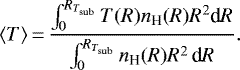$〈 T 〉 = \frac{\int_{0}^{R_{T_{sub}}} T (R) n_{H} (R) R^{2} d R}{\int_{0}^{R_{T_{sub}}} n_{H} (R) R^{2} d R} .$ $\begin{equation*} \langle T\rangle\,{=}\,\frac{\int_{0}^{R_{T_{\textrm{sub}}}} T(R) n_{\textrm{H}}(R)R^{2}\textrm{d}R}{\int_{0}^{R_{T_{\textrm{sub}}}} n_{\textrm{H}}(R)R^{2}\,\textrm{d}R}. \end{equation*}$ (B.11)

Using Eqs. (B.1), (B.2), and (B.3), one can find the above average temperature as $〈 T 〉 = 1.36 T_{sub} .$ $\begin{equation*} \langle T\rangle\,{=}\,1.36\ T_{\textrm{sub}}. \end{equation*}$ (B.12)

Therefore, the measured excitation temperature of a species would be 1.36 times the sublimation temperature of that molecule.

Appendix C Spectral fitting results

The fitted models are presented in Figs. C.1 to C.25 for B1-c and S68N. To derive the most accurate excitation temperatures, the χ² plot for each molecule is examined. Figure C.28 shows the χ² plot for one of the molecules (C₂H₅CN) where the χ² calculation is most constraining. When the χ² method wasnot constraining or the results from fitting the spectrum by eye were not consistent with the χ² results, the spectrum was fitted by eye. The fit by eye was done by fixing the column density to the best fitted value or changing it slightly around the best fitted value while varying the temperature in steps of 10 K to find the best fit. Errors of ~ 50 K to ~ 100 K were typically found. All the excitation temperatures that were not fixed were fitted by eye due to line blending. Figures C.1–C.14 and C.15–C.25 present the range of fitted models for B1-c andS68N, including the upper and lower limit temperature fit for each molecule where the fit-by-eye method was used (NH₂CHO, C₂H₅CN, HN¹³CO, CH₂DCN, and CHD₂CN towards B1-c and C₂H₅CN and CH₂DCN towards S68N).

In general, the model, as expected, does not predict a line for transitions with low A_ij. This can be seen for the NH₂CHO line with an E_up of 23.6 K and an A_ij of 1.2 × 10⁻⁵ (Figs. C.6 and C.7). Moreover, the line with an E_up of 478.0 K has a large error in its frequency in the JPL catalogue and hence is not used in the fit.

In the specific case of C₂H₅CN towards B1-c (Figs. C.4 and C.5), the two lines with upper energy levels of 153.7 K and 233.6 K have the same frequencies and plausible A_ij of 4.99 × 10⁻⁴ and 4.07 × 10⁻⁴, respectively. Hence it is not possible to say which of them is responsible for the emission line. We produced two models with the best-fit parameters for this molecule, once limiting the E_up of lines included in the model to below 160 K and once to above this value to make sure that these two models do not include the two lines at the same time. We found that the two models show very similar line peak intensities, and thus the final best-fit model most likely includes emission from both of these lines.

Fig. C.1

Model to combined Band 5 and 6 data of HN¹³CO for B1-c in red and data in black. The model uses the lower limit on the excitation temperature of HN¹³ CO. Each graph shows one line of HN¹³CO, indicated by the solid green line at the top of the box, along with its upper energy level, written in red at the top right. The lines with upper energy levels above 1000 K and/or A_ij below 10⁻⁵ are not plotted. The excitation temperature used for the figure is shown at the top left. The dashed green line shows the 3σ level. Cases where a line is seen at the 3σ level or above and is used as part of the fitting are marked with a green X at the top right corner of the box.

Fig. C.2

Same as Fig. C.1 but for its upper limit on temperature.

Fig. C.3

Same as Fig. C.1 but for DNCO and the best-fit model where the temperature is fixed.

Fig. C.4

Same as Fig. C.1 but for C₂H₅CN.

Fig. C.5

Same as Fig. C.1 but for C₂H₅CN and for its upper limit on temperature.

Fig. C.6

Same as Fig. C.1 but for NH₂CHO. The more transparent red line shows the model with a T_ex of 50 K to show that it overestimates the line with an E_up of 45.4 K.

Fig. C.7

Same as Fig. C.1 but for NH₂CHO and a high temperature for the model. This graph is presented to demonstrate that it is not possible to derive an upper limit for theexcitation temperature of this molecule because the model used in this plot is very similar to the model in Fig. C.6.

Fig. C.8

Same as Fig. C.1 but for CH₂DCN.

Fig. C.9

Same as Fig. C.1 but for CH₂DCN and for its upper limit on temperature.

Fig. C.10

Same as Fig. C.1 but for CHD₂CN.

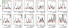Fig. C.11

Same as Fig. C.1 but for CHD₂CN and a high temperature for the model. This graph is presented to demonstrate that it is not possible to derive an upper limit for theexcitation temperature of this molecule because the model used in this plot is very similar to the model in Fig. C.10.

Fig. C.12

Same as Fig. C.1 but for NH₂CN and the best-fit model where the temperature is fixed.

Fig. C.13

Same as Fig. C.1 but for CH₃NCO and the best-fit model where the temperature is fixed.

Fig. C.14

Same as Fig. C.1 but for CH₃NH₂ and the best-fit model where the temperature is fixed.

Fig. C.15

Model to Band 6 data of HN¹³CO for S68N in red and data in black. The model uses an excitation temperature that is fixed for HN¹³ CO. Each graph shows one line of HN¹³CO, indicatedby the solid green line at the top middle along with its upper energy level at the top right. The lines with upper energy levels above 1000 K and/or A_ij below 10⁻⁵ are not plotted. The excitation temperature used for this figure is shown at the top left. The dashed green line shows the 3σ level. Cases where a line is seen at the 3σ level or above and is used as part of the fitting are marked with a green X at the top right corner of the box.

Fig. C.16

Same as Fig. C.15 but for DNCO.

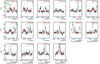Fig. C.17

Same as Fig. C.15 but for C₂H₅CN and the excitation temperature used is the lower limit for C₂H₅CN.

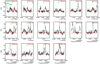Fig. C.18

Same as Fig. C.15 but for C₂H₅CN and the excitation temperature used is the upper limit for C₂H₅CN.

Fig. C.19

Same as Fig. C.15 but for NH₂CHO.

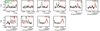Fig. C.20

Same as Fig. C.15 but for CH₂DCN and the excitation temperature used is the lower limit for CH₂DCN.

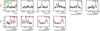Fig. C.21

Same as Fig. C.15 but for CH₂DCN and the excitation temperature used is the upper limit for CH₂DCN.

Fig. C.22

Same as Fig. C.15 but for CHD₂CN.

Fig. C.23

Same as Fig. C.15 but for NH₂CN.

Fig. C.24

Same as Fig. C.15 but for CH₃NCO.

Fig. C.25

Same as Fig. C.15 but for CH₃NH₂.

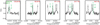Fig. C.26

Spectrum for CH₃CN towards B1-c in the Band 3 data. The upper energy levels of each line are shown at the top right of each panel.

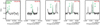Fig. C.27

Spectrum for CH₃CN towards S68N in the Band 3 data. The upper energy levels of each line are shown at the top right of each panel.

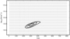Fig. C.28

χ² plot for C₂H₅CN for B1-c in the Band 5 and 6 data. The dots in the background show the grid used for this molecule, and the contours show the 3σ, 2σ, and σ levels of the best fit. It is seen that T_ex is constrained to between ~200 K and ~ 400 K, whereas the column density is well determined at (5.8 ± 1.7) × 10¹⁴. We note that the vibrational correction factor is not taken into account for this plot.

Appendix D Additional tables

Table D.1

Observational parameters of the data from observing programme 2017.1.01174.S.

Table D.2

Frequency ranges covered in the Band 5 and 6 data.

Table D.3

Characteristics of the present lines towards B1-c.

Table D.4

Characteristics of the present lines towards S68N.

Table D.5

Lines of the species in the Band 3 data.

Table D.6

Lines of the species in the Band 5 and 6 data.

References

Adams, F. C., & Shu, F. H. 1985, ApJ, 296, 655 [Google Scholar]
Aikawa, Y., & Herbst, E. 1999, ApJ, 526, 314 [Google Scholar]
Altwegg, K., Balsiger, H., Hänni, N., et al. 2020, Nat. Astron., 4, 533 [Google Scholar]
Anderson, D. E., Bergin, E. A., Maret, S., & Wakelam, V. 2013, ApJ, 779, 141 [Google Scholar]
Anttila, R., Horneman, V. M., Koivusaari, M., & Paso, R. 1993, J. Mol. Spectr., 157, 198 [Google Scholar]
Barone, V., Latouche, C., Skouteris, D., et al. 2015, MNRAS, 453, L31 [Google Scholar]
Belloche, A., Garrod, R. T., Müller, H. S. P., et al. 2009, A&A, 499, 215 [NASA ADS] [CrossRef] [EDP Sciences] [Google Scholar]
Belloche, A., Müller, H. S. P., Menten, K. M., Schilke, P., & Comito, C. 2013, A&A, 559, A47 [NASA ADS] [CrossRef] [EDP Sciences] [Google Scholar]
Belloche, A., Müller, H. S. P., Garrod, R. T., & Menten, K. M. 2016, A&A, 587, A91 [NASA ADS] [CrossRef] [EDP Sciences] [Google Scholar]
Belloche, A., Maury, A. J., Maret, S., et al. 2020, A&A, 635, A198 [CrossRef] [EDP Sciences] [Google Scholar]
Bergner, J. B., Öberg, K. I., Garrod, R. T., & Graninger, D. M. 2017, ApJ, 841, 120 [NASA ADS] [CrossRef] [Google Scholar]
Bertin, M., Fayolle, E. C., Romanzin, C., et al. 2013, ApJ, 779, 120 [Google Scholar]
Bianchi, E., Codella, C., Ceccarelli, C., et al. 2019, MNRAS, 483, 1850 [Google Scholar]
Bisschop, S. E., Jørgensen, J. K., van Dishoeck, E. F., & de Wachter, E. B. M. 2007, A&A, 465, 913 [NASA ADS] [CrossRef] [EDP Sciences] [Google Scholar]
Bisschop, S. E., Jørgensen, J. K., Bourke, T. L., Bottinelli, S., & van Dishoeck, E. F. 2008, A&A, 488, 959 [NASA ADS] [CrossRef] [EDP Sciences] [Google Scholar]
Blake, G. A., Sutton, E. C., Masson, C. R., & Phillips, T. G. 1987, ApJ, 315, 621 [Google Scholar]
Bocquet, R., Wlodarczak, G., Bauer, A., & Demaison, J. 1988, J. Mol. Spectr., 127, 382 [Google Scholar]
Bøgelund, E. G., Barr, A. G., Taquet, V., et al. 2019a, A&A, 628, A2 [NASA ADS] [CrossRef] [EDP Sciences] [Google Scholar]
Bøgelund, E. G., McGuire, B. A., Hogerheijde, M. R., van Dishoeck, E. F., & Ligterink, N. F. W. 2019b, A&A, 624, A82 [EDP Sciences] [Google Scholar]
Boogert, A. C. A., Pontoppidan, K. M., Knez, C., et al. 2008, ApJ, 678, 985 [NASA ADS] [CrossRef] [Google Scholar]
Boogert, A. C. A., Gerakines, P. A., & Whittet, D. C. B. 2015, ARA&A, 53, 541 [Google Scholar]
Bossa, J. B., Theule, P., Duvernay, F., & Chiavassa, T. 2009, ApJ, 707, 1524 [Google Scholar]
Bottinelli, S., Ceccarelli, C., Lefloch, B., et al. 2004a, ApJ, 615, 354 [Google Scholar]
Bottinelli, S., Ceccarelli, C., Neri, R., et al. 2004b, ApJ, 617, L69 [Google Scholar]
Bottinelli, S., Ceccarelli, C., Neri, R., & Williams, J. P. 2008, in IAU Symposium, 251, Organic Matter in Space, eds. S. Kwok, & S. Sanford, 117 [Google Scholar]
Boudin, N., Schutte, W. A., & Greenberg, J. M. 1998, A&A, 331, 749 [NASA ADS] [Google Scholar]
Brauer, C. S., Pearson, J. C., Drouin, B. J., & Yu, S. 2009, ApJS, 184, 133 [NASA ADS] [CrossRef] [Google Scholar]
Brown, P. D., & Millar, T. J. 1989, MNRAS, 237, 661 [NASA ADS] [Google Scholar]
Bulak, M., Paardekooper, D. M., Fedoseev, G., & Linnartz, H. 2021, A&A, 647, A82 [CrossRef] [EDP Sciences] [Google Scholar]
Calcutt, H., Jørgensen, J. K., Müller, H. S. P., et al. 2018, A&A, 616, A90 [NASA ADS] [CrossRef] [EDP Sciences] [Google Scholar]
Cazaux, S., Tielens, A. G. G. M., Ceccarelli, C., et al. 2003, ApJ, 593, L51 [NASA ADS] [CrossRef] [Google Scholar]
Cazzoli, G., & Puzzarini, C. 2006, J. Mol. Spectr., 240, 153 [NASA ADS] [CrossRef] [Google Scholar]
Ceccarelli, C., Caselli, P., Bockelée-Morvan, D., et al. 2014, in Protostars and Planets VI, eds. H. Beuther, R. S. Klessen, C. P. Dullemond, & T. Henning, 859 [Google Scholar]
Ceccarelli, C., Caselli, P., Fontani, F., et al. 2017, ApJ, 850, 176 [NASA ADS] [CrossRef] [Google Scholar]
Cernicharo, J., Kisiel, Z., Tercero, B., et al. 2016, A&A, 587, A4 [NASA ADS] [CrossRef] [EDP Sciences] [Google Scholar]
Codella, C., Ceccarelli, C., Caselli, P., et al. 2017, A&A, 605, A3 [NASA ADS] [CrossRef] [EDP Sciences] [Google Scholar]
Collings, M. P., Anderson, M. A., Chen, R., et al. 2004, MNRAS, 354, 1133 [NASA ADS] [CrossRef] [Google Scholar]
Costain, C. C., & Dowling, J. M. 1960, J. Chem. Phys., 32, 158 [NASA ADS] [CrossRef] [Google Scholar]
Coutens,A., Jørgensen, J. K., van der Wiel, M. H. D., et al. 2016, A&A, 590, A6 [NASA ADS] [CrossRef] [EDP Sciences] [Google Scholar]
Coutens, A., Willis, E. R., Garrod, R. T., et al. 2018, A&A, 612, A107 [NASA ADS] [CrossRef] [EDP Sciences] [Google Scholar]
Crimier, N., Ceccarelli, C., Alonso-Albi, T., et al. 2010, A&A, 516, A102 [NASA ADS] [CrossRef] [EDP Sciences] [Google Scholar]
Crockett, N. R., Bergin, E. A., Neill, J. L., et al. 2015, ApJ, 806, 239 [NASA ADS] [CrossRef] [Google Scholar]
Csengeri, T., Belloche, A., Bontemps, S., et al. 2019, A&A, 632, A57 [NASA ADS] [CrossRef] [EDP Sciences] [Google Scholar]
Cuppen, H. M., Walsh, C., Lamberts, T., et al. 2017, Space Sci. Rev., 212, 1 [Google Scholar]
De Simone, M., Ceccarelli, C., Codella, C., et al. 2020, ApJ, 896, L3 [CrossRef] [Google Scholar]
Dulieu, F., Nguyen, T., Congiu, E., Baouche, S., & Taquet, V. 2019, MNRAS, 484, L119 [NASA ADS] [CrossRef] [Google Scholar]
Enoch, M. L., Corder, S., Duchêne, G., et al. 2011, ApJS, 195, 21 [NASA ADS] [CrossRef] [Google Scholar]
Fedoseev, G., Ioppolo, S., Zhao, D., Lamberts, T., & Linnartz, H. 2015, MNRAS, 446, 439 [NASA ADS] [CrossRef] [Google Scholar]
Fedoseev, G., Chuang, K. J., van Dishoeck, E. F., Ioppolo, S., & Linnartz, H. 2016, MNRAS, 460, 4297 [NASA ADS] [CrossRef] [Google Scholar]
Fedoseev, G., Chuang, K. J., Ioppolo, S., et al. 2017, ApJ, 842, 52 [NASA ADS] [CrossRef] [Google Scholar]
Ferrero, S., Zamirri, L., Ceccarelli, C., et al. 2020, ApJ, 904, 11 [CrossRef] [Google Scholar]
Fontani, F., Pascucci, I., Caselli, P., et al. 2007, A&A, 470, 639 [NASA ADS] [CrossRef] [EDP Sciences] [Google Scholar]
Fuchs, G. W., Cuppen, H. M., Ioppolo, S., et al. 2009, A&A, 505, 629 [NASA ADS] [CrossRef] [EDP Sciences] [Google Scholar]
Fukuyama, Y., Odashima, H., Takagi, K., & Tsunekawa, S. 1996, ApJS, 104, 329 [NASA ADS] [CrossRef] [Google Scholar]
Furuya, K., van Dishoeck, E. F., & Aikawa, Y. 2016, A&A, 586, A127 [NASA ADS] [CrossRef] [EDP Sciences] [Google Scholar]
Gadhi, J., Lahrouni, A., Legrand, J., & Demaison, J. 1995, J. Chim. Phys., 92, 1984 [Google Scholar]
Garrod, R. T. 2013, ApJ, 765, 60 [Google Scholar]
Garrod, R. T., Widicus Weaver, S. L., & Herbst, E. 2008, ApJ, 682, 283 [NASA ADS] [CrossRef] [Google Scholar]
Gerakines, P. A., & Hudson, R. L. 2020, ApJ, 901, 52 [CrossRef] [Google Scholar]
Gibb, E., Nummelin, A., Irvine, W. M., Whittet, D. C. B., & Bergman, P. 2000, ApJ, 545, 309 [NASA ADS] [CrossRef] [PubMed] [Google Scholar]
Grim, R. J. A., & Greenberg, J. M. 1987, ApJ, 321, L91 [NASA ADS] [CrossRef] [Google Scholar]
Grim, R. J. A., Baas, F., Geballe, T. R., Greenberg, J. M., & Schutte, W. A. 1991, A&A, 243, 473 [NASA ADS] [Google Scholar]
Halonen, L., & Mills, I. M. 1978, J. Mol. Spectr., 73, 494 [NASA ADS] [CrossRef] [Google Scholar]
Harsono, D., van Dishoeck, E. F., Bruderer, S., Li, Z. Y., & Jørgensen, J. K. 2015, A&A, 577, A22 [NASA ADS] [CrossRef] [EDP Sciences] [Google Scholar]
Harsono, D., Bjerkeli, P., van der Wiel, M. H. D., et al. 2018, Nat. Astron., 2, 646 [NASA ADS] [CrossRef] [Google Scholar]
Hasegawa, T. I., Herbst, E., & Leung, C. M. 1992, ApJS, 82, 167 [NASA ADS] [CrossRef] [Google Scholar]
Haupa, K. A., Tarczay, G., & Lee, Y.-P. 2019, J. Am. Chem. Soc., 141, 11614 [CrossRef] [Google Scholar]
Heise, H. M., Winther, F., & Lutz, H. 1981, J. Mol. Spectr., 90, 531 [NASA ADS] [CrossRef] [Google Scholar]
Hocking, W. H., Gerry, M. C. L., & Winnewisser, G. 1975, Can. J. Phys., 53, 1869 [NASA ADS] [CrossRef] [Google Scholar]
Ilee, J. D., Cyganowski, C. J., Nazari, P., et al. 2016, MNRAS, 462, 4386 [NASA ADS] [CrossRef] [Google Scholar]
Ilyushin, V. V., Alekseev, E. A., Dyubko, S. F., Motiyenko, R. A., & Hougen, J. T. 2005, J. Mol. Spectr., 229, 170 [NASA ADS] [CrossRef] [Google Scholar]
Imai, M., Sakai, N., Oya, Y., et al. 2016, ApJ, 830, L37 [NASA ADS] [CrossRef] [Google Scholar]
Isokoski, K., Bottinelli, S., & van Dishoeck, E. F. 2013, A&A, 554, A100 [NASA ADS] [CrossRef] [EDP Sciences] [Google Scholar]
Johnson, D. R., Lovas, F. J., & Kirchhoff, W. H. 1972, J. Phys. Chem. Ref. Data, 1, 1011 [NASA ADS] [CrossRef] [Google Scholar]
Jones, B. M., Bennett, C. J., & Kaiser, R. I. 2011, ApJ, 734, 78 [NASA ADS] [CrossRef] [Google Scholar]
Jørgensen, J. K., Schöier, F. L., & van Dishoeck, E. F. 2002, A&A, 389, 908 [NASA ADS] [CrossRef] [EDP Sciences] [Google Scholar]
Jørgensen, J. K., Harvey, P. M., Evans, Neal J., I., et al. 2006, ApJ, 645, 1246 [NASA ADS] [CrossRef] [Google Scholar]
Jørgensen, J. K., van der Wiel, M. H. D., Coutens, A., et al. 2016, A&A, 595, A117 [NASA ADS] [CrossRef] [EDP Sciences] [Google Scholar]
Jørgensen, J. K., Müller, H. S. P., Calcutt, H., et al. 2018, A&A, 620, A170 [NASA ADS] [CrossRef] [EDP Sciences] [Google Scholar]
Jørgensen, J. K., Belloche, A., & Garrod, R. T. 2020, ARA&A, 58, 727 [Google Scholar]
Karska, A., Kaufman, M. J., Kristensen, L. E., et al. 2018, ApJS, 235, 30 [Google Scholar]
Kirchhoff, W. H. 1972, J. Mol. Spectr., 41, 333 [CrossRef] [Google Scholar]
Kirchhoff, W. H., & Johnson, D. R. 1973, J. Mol. Spectr., 45, 159 [NASA ADS] [CrossRef] [Google Scholar]
Koivusaari, M., Horneman, V. M., & Anttila, R. 1992, J. Mol. Spectr., 152, 377 [NASA ADS] [CrossRef] [Google Scholar]
Koput, J. 1986, J. Mol. Spectr., 115, 131 [NASA ADS] [CrossRef] [Google Scholar]
Kréglewski, M., & Wlodarczak, G. 1992, J. Mol. Spectr., 156, 383 [NASA ADS] [CrossRef] [Google Scholar]
Krȩglewski, M., Stahl, W., Grabow, J.-U., & Wlodarczak, G. 1992, Chem. Phys. Lett., 196, 155 [NASA ADS] [CrossRef] [Google Scholar]
Kukolich, S. G., & Nelson, A. C. 1971, Chem. Phys. Lett., 11, 383 [NASA ADS] [CrossRef] [Google Scholar]
Kukolich, S. G., Nelson, A. C., & Yamanashi, B. S. 1971, J. Am. Chem. Soc., 93, 6769 [CrossRef] [Google Scholar]
Kurland, R. J., & Wilson, E. B. 1957, J. Chem. Phys., 27, 585 [NASA ADS] [CrossRef] [Google Scholar]
Lapinov, A. V., Golubiatnikov, G. Y., Markov, V. N., & Guarnieri, A. 2007, Astron. Lett., 33, 121 [NASA ADS] [CrossRef] [Google Scholar]
Le Guennec, M., Wlodarczak, G., Burie, J., & Demaison, J. 1992, J. Mol. Spectr., 154, 305 [NASA ADS] [CrossRef] [Google Scholar]
Lee, C.-F., Codella, C., Li, Z.-Y., & Liu, S.-Y. 2019, ApJ, 876, 63 [NASA ADS] [CrossRef] [Google Scholar]
Lide, David R., J. 1954, J. Chem. Phys., 22, 1613 [NASA ADS] [CrossRef] [Google Scholar]
Lide, David R., J. 1957, J. Chem. Phys., 27, 343 [NASA ADS] [CrossRef] [Google Scholar]
Ligterink, N. F. W., Coutens, A., Kofman, V., et al. 2017, MNRAS, 469, 2219 [NASA ADS] [CrossRef] [Google Scholar]
Ligterink, N. F. W., Calcutt, H., Coutens, A., et al. 2018, A&A, 619, A28 [NASA ADS] [CrossRef] [EDP Sciences] [Google Scholar]
Ligterink, N. F. W., El-Abd, S. J., Brogan, C. L., et al. 2020, ApJ, 901, 37 [Google Scholar]
Linnartz, H., Ioppolo, S., & Fedoseev, G. 2015, Int. Rev. Phys. Chem., 34, 205 [CrossRef] [Google Scholar]
López-Sepulcre, A., Sakai, N., Neri, R., et al. 2017, A&A, 606, A121 [NASA ADS] [CrossRef] [EDP Sciences] [Google Scholar]
López-Sepulcre, A., Balucani, N., Ceccarelli, C., et al. 2019, ACS Earth Space Chem., 3, 2122 [CrossRef] [Google Scholar]
Manara, C. F., Morbidelli, A., & Guillot, T. 2018, A&A, 618, L3 [NASA ADS] [CrossRef] [EDP Sciences] [Google Scholar]
Manigand, S., Jørgensen, J. K., Calcutt, H., et al. 2020, A&A, 635, A48 [NASA ADS] [CrossRef] [EDP Sciences] [Google Scholar]
Marcelino, N., Gerin, M., Cernicharo, J., et al. 2018, A&A, 620, A80 [NASA ADS] [CrossRef] [EDP Sciences] [Google Scholar]
Maret, S., Maury, A. J., Belloche, A., et al. 2020, A&A, 635, A15 [NASA ADS] [CrossRef] [EDP Sciences] [Google Scholar]
Margulès, L., McGuire, B. A., Senent, M. L., et al. 2017, A&A, 601, A50 [CrossRef] [EDP Sciences] [Google Scholar]
Martín-Doménech, R., Bergner, J. B., Öberg, K. I., & Jørgensen, J. K. 2019, ApJ, 880, 130 [CrossRef] [Google Scholar]
Martín-Doménech, R., Öberg, K. I., & Rajappan, M. 2020, ApJ, 894, 98 [Google Scholar]
Milam, S. N., Savage, C., Brewster, M. A., Ziurys, L. M., & Wyckoff, S. 2005, ApJ, 634, 1126 [NASA ADS] [CrossRef] [Google Scholar]
Müller, H. S. P., Thorwirth, S., Roth, D. A., & Winnewisser, G. 2001, A&A, 370, L49 [NASA ADS] [CrossRef] [EDP Sciences] [Google Scholar]
Müller, H. S. P., Schlöder, F., Stutzki, J., & Winnewisser, G. 2005, J. Mol. Struct., 742, 215 [Google Scholar]
Müller, H. S. P., Drouin, B. J., & Pearson, J. C. 2009, A&A, 506, 1487 [NASA ADS] [CrossRef] [EDP Sciences] [Google Scholar]
Müller, H. S. P., Brown, L. R., Drouin, B. J., et al. 2015, J. Mol. Spectr., 312, 22 [NASA ADS] [CrossRef] [Google Scholar]
Murillo, N. M., Lai, S.-P., Bruderer, S., Harsono, D., & van Dishoeck, E. F. 2013, A&A, 560, A103 [NASA ADS] [CrossRef] [EDP Sciences] [Google Scholar]
Murillo, N. M., van Dishoeck, E. F., van der Wiel, M. H. D., et al. 2018, A&A, 617, A120 [NASA ADS] [CrossRef] [EDP Sciences] [Google Scholar]
Nguyen, L., Walters, A., Margulès, L., et al. 2013, A&A, 553, A84 [NASA ADS] [CrossRef] [EDP Sciences] [Google Scholar]
Niedenhoff, M., Yamada, K. M. T., Belov, S. P., & Winnewisser, G. 1995, J. Mol. Spectr., 174, 151 [NASA ADS] [CrossRef] [Google Scholar]
Nishikawa, T. 1957, J. Phys. Soc. Jpn., 12, 668 [NASA ADS] [CrossRef] [Google Scholar]
Noble, J. A., Theule, P., Congiu, E., et al. 2015, A&A, 576, A91 [NASA ADS] [CrossRef] [EDP Sciences] [Google Scholar]
Nummelin, A., Bergman, P., Hjalmarson, Å., et al. 2000, ApJS, 128, 213 [NASA ADS] [CrossRef] [Google Scholar]
Öberg, K. I., Garrod, R. T., van Dishoeck, E. F., & Linnartz, H. 2009a, A&A, 504, 891 [NASA ADS] [CrossRef] [EDP Sciences] [Google Scholar]
Öberg, K. I., van Dishoeck, E. F., & Linnartz, H. 2009b, A&A, 496, 281 [NASA ADS] [CrossRef] [EDP Sciences] [Google Scholar]
Öberg, K. I., Boogert, A. C. A., Pontoppidan, K. M., et al. 2011, ApJ, 740, 109 [NASA ADS] [CrossRef] [Google Scholar]
Ohashi, N., Takagi, K., Hougen, J. T., Olson, W. B., & Lafferty, W. J. 1987, J. Mol. Spectr., 126, 443 [NASA ADS] [CrossRef] [Google Scholar]
Ortiz-León, G. N., Dzib, S. A., Kounkel, M. A., et al. 2017, ApJ, 834, 143 [Google Scholar]
Ortiz-León, G. N., Loinard, L., Dzib, S. A., et al. 2018, ApJ, 865, 73 [Google Scholar]
Oya, Y., Sakai, N., Watanabe, Y., et al. 2017, ApJ, 837, 174 [NASA ADS] [CrossRef] [Google Scholar]
Pearson, J. C., Sastry, K. V. L. N., Herbst, E., & De Lucia, F. C. 1994, ApJS, 93, 589 [NASA ADS] [CrossRef] [Google Scholar]
Penteado, E. M., Walsh, C., & Cuppen, H. M. 2017, ApJ, 844, 71 [NASA ADS] [CrossRef] [Google Scholar]
Persson, M. V., Harsono, D., Tobin, J. J., et al. 2016, A&A, 590, A33 [NASA ADS] [CrossRef] [EDP Sciences] [Google Scholar]
Pickett, H. M., Poynter, R. L., Cohen, E. A., et al. 1998, J. Quant. Spec. Rad. Transf., 60, 883 [Google Scholar]
Podio, L., Codella, C., Gueth, F., et al. 2015, A&A, 581, A85 [NASA ADS] [CrossRef] [EDP Sciences] [Google Scholar]
Prodanović, T., Steigman, G., & Fields, B. D. 2010, MNRAS, 406, 1108 [NASA ADS] [Google Scholar]
Qasim, D., Fedoseev, G., Chuang, K. J., et al. 2019, A&A, 627, A1 [NASA ADS] [CrossRef] [EDP Sciences] [Google Scholar]
Raunier, S., Chiavassa, T., Duvernay, F., et al. 2004, A&A, 416, 165 [NASA ADS] [CrossRef] [EDP Sciences] [Google Scholar]
Read, W. G., Cohen, E. A., & Pickett, H. M. 1986, J. Mol. Spectr., 115, 316 [Google Scholar]
Rimola, A., Skouteris, D., Balucani, N., et al. 2018, ACS Earth Space Chem., 2, 720 [Google Scholar]
Roberts, H., Herbst, E., & Millar, T. J. 2003, ApJ, 591, L41 [Google Scholar]
Schöier, F. L., Jørgensen, J. K., van Dishoeck, E. F., & Blake, G. A. 2002, A&A, 390, 1001 [NASA ADS] [CrossRef] [EDP Sciences] [Google Scholar]
Schutte, W. A., & Khanna, R. K. 2003, A&A, 398, 1049 [NASA ADS] [CrossRef] [EDP Sciences] [Google Scholar]
Schutte, W. A., Boogert, A. C. A., Tielens, A. G. G. M., et al. 1999, A&A, 343, 966 [NASA ADS] [Google Scholar]
Shimoda, K., Nishikawa, T., & Itoh, T. 1954, J. Phys. Soc. Jpn., 9, 974 [NASA ADS] [CrossRef] [Google Scholar]
Šimečková, M., Urban, Š., Fuchs, U., et al. 2004, J. Mol. Spectr., 226, 123 [NASA ADS] [CrossRef] [Google Scholar]
Sipilä, O., Caselli, P., & Harju, J. 2015, A&A, 578, A55 [NASA ADS] [CrossRef] [EDP Sciences] [Google Scholar]
Skouteris, D., Vazart, F., Ceccarelli, C., et al. 2017, MNRAS, 468, L1 [NASA ADS] [Google Scholar]
Song, L., & Kästner, J. 2016, Phys. Chem. Chem. Phys. (Incorp. Faraday Trans.), 18, 29278 [NASA ADS] [CrossRef] [Google Scholar]
Taban, I. M., Schutte, W. A., Pontoppidan, K. M., & van Dishoeck, E. F. 2003, A&A, 399, 169 [NASA ADS] [CrossRef] [EDP Sciences] [Google Scholar]
Takagi, K., & Kojima, T. 1971, J. Phys. Soc. Jpn., 30, 1145 [NASA ADS] [CrossRef] [Google Scholar]
Taniguchi, K., Guzmán, A. E., Majumdar, L., Saito, M., & Tokuda, K. 2020, ApJ, 898, 54 [Google Scholar]
Taquet, V., Ceccarelli, C., & Kahane, C. 2012, ApJ, 748, L3 [NASA ADS] [CrossRef] [Google Scholar]
Taquet, V., Charnley, S. B., & Sipilä, O. 2014, ApJ, 791, 1 [Google Scholar]
Taquet, V., López-Sepulcre, A., Ceccarelli, C., et al. 2015, ApJ, 804, 81 [NASA ADS] [CrossRef] [Google Scholar]
Taquet, V., Bianchi, E., Codella, C., et al. 2019, A&A, 632, A19 [CrossRef] [EDP Sciences] [Google Scholar]
Terwisscha van Scheltinga, J., Ligterink, N. F. W., Boogert, A. C. A., van Dishoeck, E. F., & Linnartz, H. 2018, A&A, 611, A35 [NASA ADS] [CrossRef] [EDP Sciences] [Google Scholar]
Tideswell, D. M., Fuller, G. A., Millar, T. J., & Markwick, A. J. 2010, A&A, 510, A85 [NASA ADS] [CrossRef] [EDP Sciences] [Google Scholar]
Tielens, A. G. G. M. 2013, Rev. Mod. Phys., 85, 1021 [Google Scholar]
Tielens, A. G. G. M., Tokunaga, A. T., Geballe, T. R., & Baas, F. 1991, ApJ, 381, 181 [NASA ADS] [CrossRef] [PubMed] [Google Scholar]
Tobin, J. J., Hartmann, L., Chiang, H.-F., et al. 2012, Nature, 492, 83 [Google Scholar]
Tobin, J. J., Sheehan, P. D., Megeath, S. T., et al. 2020, ApJ, 890, 130 [Google Scholar]
Tolonen, A. M., Koivusaari, M., Paso, R., et al. 1993, J. Mol. Spectr., 160, 554 [NASA ADS] [CrossRef] [Google Scholar]
Tychoniec, Ł., Tobin, J. J., Karska, A., et al. 2018, ApJS, 238, 19 [NASA ADS] [CrossRef] [Google Scholar]
Tychoniec, Ł., Hull, C. L. H., Kristensen, L. E., et al. 2019, A&A, 632, A101 [NASA ADS] [CrossRef] [EDP Sciences] [Google Scholar]
Tychoniec, Ł., Manara, C. F., Rosotti, G. P., et al. 2020, A&A, 640, A19 [CrossRef] [EDP Sciences] [Google Scholar]
van Broekhuizen, F. A., Keane, J. V., & Schutte, W. A. 2004, A&A, 415, 425 [NASA ADS] [CrossRef] [EDP Sciences] [Google Scholar]
van Broekhuizen, F. A., Pontoppidan, K. M., Fraser, H. J., & van Dishoeck, E. F. 2005, A&A, 441, 249 [NASA ADS] [CrossRef] [EDP Sciences] [Google Scholar]
van Dishoeck, E. F., Blake, G. A., Jansen, D. J., & Groesbeck, T. D. 1995, ApJ, 447, 760 [NASA ADS] [CrossRef] [Google Scholar]
van Gelder, M. L., Tabone, B., Tychoniec, Ł., et al. 2020, A&A, 639, A87 [CrossRef] [EDP Sciences] [Google Scholar]
van ’t Hoff, M. L. R., Bergin, E. A., Jørgensen, J. K., & Blake, G. A. 2020a, ApJ, 897, L38 [Google Scholar]
van ’t Hoff, M. L. R., Harsono, D., Tobin, J. J., et al. 2020b, ApJ, 901, 166 [CrossRef] [Google Scholar]
van ’t Hoff, M. L. R., van Dishoeck, E. F., Jørgensen, J. K., & Calcutt, H. 2020c, A&A, 633, A7 [CrossRef] [EDP Sciences] [Google Scholar]
Vastel, C., Bottinelli, S., Caux, E., Glorian, J. M., & Boiziot, M. 2015, in SF2A-2015: Proceedings of the Annual Meeting of the French Society of Astronomy and Astrophysics, 313 [Google Scholar]
Vazart, F., Ceccarelli, C., Balucani, N., Bianchi, E., & Skouteris, D. 2020, MNRAS, 499, 5547 [Google Scholar]
Watanabe, N., & Kouchi, A. 2002, ApJ, 571, L173 [Google Scholar]
Watson, W. D. 1976, Rev. Mod. Phys., 48, 513 [Google Scholar]
Wilson, T. L., & Rood, R. 1994, ARA&A, 32, 191 [NASA ADS] [CrossRef] [Google Scholar]
Wright, G. S., Wright, D., Goodson, G. B., et al. 2015, PASP, 127, 595 [Google Scholar]
Yıldız, U. A., Kristensen, L. E., van Dishoeck, E. F., et al. 2013, A&A, 556, A89 [NASA ADS] [CrossRef] [EDP Sciences] [Google Scholar]

¹

http://cassis.irap.omp.eu/

All Tables

Table 1

Column densities and excitation temperatures for B1-c and S68N in a 0.45′′ beam.

In the text

Table D.1

Observational parameters of the data from observing programme 2017.1.01174.S.

In the text

Table D.2

Frequency ranges covered in the Band 5 and 6 data.

In the text

Table D.3

Characteristics of the present lines towards B1-c.

In the text

Table D.4

Characteristics of the present lines towards S68N.

In the text

Table D.5

Lines of the species in the Band 3 data.

In the text

Table D.6

Lines of the species in the Band 5 and 6 data.

In the text

All Figures

Fig. 1

Best fitted model to combined Band 5 and 6 NH₂CHO data for B1-c in red and data in black. Each graph shows one line of NH₂CHO with its upper state energy level and the A_ij coefficient at the top right in red and blue, respectively. The dashed green line indicates the 3σ level. The lines above the 3σ level that were used in the fitting are indicated by a green X. The lines with upper energy levels above 1000 K and/or A_ij below 10⁻⁵ are not plotted.

In the text

	Fig. 2 Same as Fig. 1 but for HN¹³CO.
In the text

Fig. 3

Moment zero maps of the lines of SO 6₇−5₆ (E_up = 47.6 K), HNCO 12_0,12−11_0,11 (E_up = 82.3 K), and NH₂CHO 13_1,13 − 12_1,12 (E_up = 91.8 K) (from left to right) for B1-c (top row) and S68N (bottom row) in the Band 6 data. The images are made by integrating over [−10, 10] km s⁻¹ with respect to V_lsr. The black contours show the continuum in levels of [15, 30, 45, 60, 75, 90, 105] σ_cont with a σ_cont of 0.2 mJy beam⁻¹ for B1-c and [30, 45, 60, 75, 90, 105, 120] σ_cont with a σ_cont of 0.09 mJy beam⁻¹ for S68N. The beam size is shown at the right-hand side of each panel. SO traces the extended outflow, while the other two molecules show compact emissions. The approximate directions of the blueshifted and redshifted emission of the outflow are shown with blue and red arrows.

In the text

Fig. 4

Excitation temperatures for N-bearing species discussed in this work (red) and O-bearing species discussed in van Gelder et al. (2020) (blue) for B1-c and S68N. Only the species with derived T_ex are plotted. The solid red and blue lines show the average values for the red and blue data points, respectively. The shaded red and blue areas show the standard deviation of the data points. The grey points show the sublimation temperatures of the corresponding molecules found by the gas-grain balance model (Hasegawa et al. 1992) and the respective binding energies of each molecule (Penteado et al. 2017; Garrod 2013).

In the text

Fig. 5

Cartoon of the temperature structure of protostellar envelopes showing where O-bearing and N-bearing species are most likely to be found in the gas. This is based on the findings of Crockett et al. (2015) for massive protostars, who showedthat higher excitation temperatures for N-bearing COMs are found towards several high-mass protostars, and van ’t Hoff et al. (2020a), who proposed a top-down carbon chemistry for nitriles. It is not yet clear whether this structure also applies to low-mass protostars.

In the text

Fig. 6

Abundance ratio of NH₂CHO and HNCO with respect to CH₃OH against source luminosity. Red points show the results for the sources considered in this work. The grey points indicate other low- and high-mass sources. These sources are IRAS 16293A (Ligterink et al. 2017; Manigand et al. 2020), IRAS 16293B (Coutens et al. 2016; Ligterink et al. 2017; Jørgensen et al. 2018), HH 212 (Lee et al. 2019), AFGL 4176 (Bøgelund et al. 2019a), and NGC6334 MM1 and MM2 (Bøgelund et al. 2019b).

In the text

Fig. 7

Column densities of the N-bearing molecules with respect to methanol for sources observed by ALMA. Column densities of methanol for B1-c and S68N are taken from van Gelder et al. (2020). Shown are IRAS 16293A (Coutens et al. 2016; Ligterink et al. 2017; Calcutt et al. 2018; Manigand et al. 2020), IRAS 16293B (Coutens et al. 2016, 2018; Ligterink et al. 2017; Jørgensen et al. 2018; Calcutt et al. 2018), HH 212 (Lee et al. 2019), AFGL 4176 (Bøgelund et al. 2019a), and NGC 6334 MM1, MM2, and MM3 (Bøgelund et al. 2019b).

In the text

	Fig. 8 Column densities of N-bearing species with respect to HNCO as derived from HN¹³ CO. Shown are IRAS 16293A (Coutens et al. 2016; Ligterink et al. 2017; Calcutt et al. 2018; Manigand et al. 2020), IRAS 16293B (Coutens et al. 2016, 2018; Ligterink et al. 2017; Calcutt et al. 2018), NGC 1333 IRAS 4A2 (López-Sepulcre et al. 2017), and AFGL 4176 (Bøgelund et al. 2019a).
In the text

Fig. 9

Correction factor, f_sub, introduced in Eq. (4) due to different emitting areas arising from the sublimation temperature. The shaded area shows where most of the species considered in this work fall on this graph (sublimation temperatures between 55 K and 125 K).The abundance ratios of these species with respect to methanol are found by multiplying their column density ratios with respect to methanol by a factor of between 0.1 and 2.

In the text

Fig. C.1

Model to combined Band 5 and 6 data of HN¹³CO for B1-c in red and data in black. The model uses the lower limit on the excitation temperature of HN¹³ CO. Each graph shows one line of HN¹³CO, indicated by the solid green line at the top of the box, along with its upper energy level, written in red at the top right. The lines with upper energy levels above 1000 K and/or A_ij below 10⁻⁵ are not plotted. The excitation temperature used for the figure is shown at the top left. The dashed green line shows the 3σ level. Cases where a line is seen at the 3σ level or above and is used as part of the fitting are marked with a green X at the top right corner of the box.

In the text

	Fig. C.2 Same as Fig. C.1 but for its upper limit on temperature.
In the text

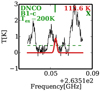	Fig. C.3 Same as Fig. C.1 but for DNCO and the best-fit model where the temperature is fixed.
In the text

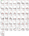	Fig. C.4 Same as Fig. C.1 but for C₂H₅CN.
In the text

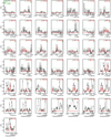	Fig. C.5 Same as Fig. C.1 but for C₂H₅CN and for its upper limit on temperature.
In the text

	Fig. C.6 Same as Fig. C.1 but for NH₂CHO. The more transparent red line shows the model with a T_ex of 50 K to show that it overestimates the line with an E_up of 45.4 K.
In the text

	Fig. C.7 Same as Fig. C.1 but for NH₂CHO and a high temperature for the model. This graph is presented to demonstrate that it is not possible to derive an upper limit for theexcitation temperature of this molecule because the model used in this plot is very similar to the model in Fig. C.6.
In the text

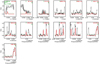	Fig. C.8 Same as Fig. C.1 but for CH₂DCN.
In the text

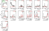	Fig. C.9 Same as Fig. C.1 but for CH₂DCN and for its upper limit on temperature.
In the text

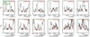	Fig. C.10 Same as Fig. C.1 but for CHD₂CN.
In the text

	Fig. C.11 Same as Fig. C.1 but for CHD₂CN and a high temperature for the model. This graph is presented to demonstrate that it is not possible to derive an upper limit for theexcitation temperature of this molecule because the model used in this plot is very similar to the model in Fig. C.10.
In the text

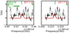	Fig. C.12 Same as Fig. C.1 but for NH₂CN and the best-fit model where the temperature is fixed.
In the text

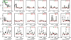	Fig. C.13 Same as Fig. C.1 but for CH₃NCO and the best-fit model where the temperature is fixed.
In the text

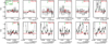	Fig. C.14 Same as Fig. C.1 but for CH₃NH₂ and the best-fit model where the temperature is fixed.
In the text

Fig. C.15

Model to Band 6 data of HN¹³CO for S68N in red and data in black. The model uses an excitation temperature that is fixed for HN¹³ CO. Each graph shows one line of HN¹³CO, indicatedby the solid green line at the top middle along with its upper energy level at the top right. The lines with upper energy levels above 1000 K and/or A_ij below 10⁻⁵ are not plotted. The excitation temperature used for this figure is shown at the top left. The dashed green line shows the 3σ level. Cases where a line is seen at the 3σ level or above and is used as part of the fitting are marked with a green X at the top right corner of the box.

In the text

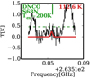	Fig. C.16 Same as Fig. C.15 but for DNCO.
In the text

	Fig. C.17 Same as Fig. C.15 but for C₂H₅CN and the excitation temperature used is the lower limit for C₂H₅CN.
In the text

	Fig. C.18 Same as Fig. C.15 but for C₂H₅CN and the excitation temperature used is the upper limit for C₂H₅CN.
In the text

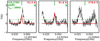	Fig. C.19 Same as Fig. C.15 but for NH₂CHO.
In the text

	Fig. C.20 Same as Fig. C.15 but for CH₂DCN and the excitation temperature used is the lower limit for CH₂DCN.
In the text

	Fig. C.21 Same as Fig. C.15 but for CH₂DCN and the excitation temperature used is the upper limit for CH₂DCN.
In the text

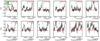	Fig. C.22 Same as Fig. C.15 but for CHD₂CN.
In the text

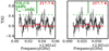	Fig. C.23 Same as Fig. C.15 but for NH₂CN.
In the text

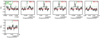	Fig. C.24 Same as Fig. C.15 but for CH₃NCO.
In the text

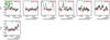	Fig. C.25 Same as Fig. C.15 but for CH₃NH₂.
In the text

	Fig. C.26 Spectrum for CH₃CN towards B1-c in the Band 3 data. The upper energy levels of each line are shown at the top right of each panel.
In the text

	Fig. C.27 Spectrum for CH₃CN towards S68N in the Band 3 data. The upper energy levels of each line are shown at the top right of each panel.
In the text

Fig. C.28

χ² plot for C₂H₅CN for B1-c in the Band 5 and 6 data. The dots in the background show the grid used for this molecule, and the contours show the 3σ, 2σ, and σ levels of the best fit. It is seen that T_ex is constrained to between ~200 K and ~ 400 K, whereas the column density is well determined at (5.8 ± 1.7) × 10¹⁴. We note that the vibrational correction factor is not taken into account for this plot.

In the text

Current usage metrics show cumulative count of Article Views (full-text article views including HTML views, PDF and ePub downloads, according to the available data) and Abstracts Views on Vision4Press platform.

Data correspond to usage on the plateform after 2015. The current usage metrics is available 48-96 hours after online publication and is updated daily on week days.

Initial download of the metrics may take a while.

[1] Adams, F. C., & Shu, F. H. 1985, ApJ, 296, 655 [Google Scholar]

[2] Aikawa, Y., & Herbst, E. 1999, ApJ, 526, 314 [Google Scholar]

[3] Altwegg, K., Balsiger, H., Hänni, N., et al. 2020, Nat. Astron., 4, 533 [Google Scholar]

[4] Anderson, D. E., Bergin, E. A., Maret, S., & Wakelam, V. 2013, ApJ, 779, 141 [Google Scholar]

[5] Anttila, R., Horneman, V. M., Koivusaari, M., & Paso, R. 1993, J. Mol. Spectr., 157, 198 [Google Scholar]

[6] Barone, V., Latouche, C., Skouteris, D., et al. 2015, MNRAS, 453, L31 [Google Scholar]

[7] Belloche, A., Garrod, R. T., Müller, H. S. P., et al. 2009, A&A, 499, 215 [NASA ADS] [CrossRef] [EDP Sciences] [Google Scholar]

[8] Belloche, A., Müller, H. S. P., Menten, K. M., Schilke, P., & Comito, C. 2013, A&A, 559, A47 [NASA ADS] [CrossRef] [EDP Sciences] [Google Scholar]

[9] Belloche, A., Müller, H. S. P., Garrod, R. T., & Menten, K. M. 2016, A&A, 587, A91 [NASA ADS] [CrossRef] [EDP Sciences] [Google Scholar]

[10] Belloche, A., Maury, A. J., Maret, S., et al. 2020, A&A, 635, A198 [CrossRef] [EDP Sciences] [Google Scholar]

[11] Bergner, J. B., Öberg, K. I., Garrod, R. T., & Graninger, D. M. 2017, ApJ, 841, 120 [NASA ADS] [CrossRef] [Google Scholar]

[12] Bertin, M., Fayolle, E. C., Romanzin, C., et al. 2013, ApJ, 779, 120 [Google Scholar]

[13] Bianchi, E., Codella, C., Ceccarelli, C., et al. 2019, MNRAS, 483, 1850 [Google Scholar]

[14] Bisschop, S. E., Jørgensen, J. K., van Dishoeck, E. F., & de Wachter, E. B. M. 2007, A&A, 465, 913 [NASA ADS] [CrossRef] [EDP Sciences] [Google Scholar]

[15] Bisschop, S. E., Jørgensen, J. K., Bourke, T. L., Bottinelli, S., & van Dishoeck, E. F. 2008, A&A, 488, 959 [NASA ADS] [CrossRef] [EDP Sciences] [Google Scholar]

[16] Blake, G. A., Sutton, E. C., Masson, C. R., & Phillips, T. G. 1987, ApJ, 315, 621 [Google Scholar]

[17] Bocquet, R., Wlodarczak, G., Bauer, A., & Demaison, J. 1988, J. Mol. Spectr., 127, 382 [Google Scholar]

[18] Bøgelund, E. G., Barr, A. G., Taquet, V., et al. 2019a, A&A, 628, A2 [NASA ADS] [CrossRef] [EDP Sciences] [Google Scholar]

[19] Bøgelund, E. G., McGuire, B. A., Hogerheijde, M. R., van Dishoeck, E. F., & Ligterink, N. F. W. 2019b, A&A, 624, A82 [EDP Sciences] [Google Scholar]

[20] Boogert, A. C. A., Pontoppidan, K. M., Knez, C., et al. 2008, ApJ, 678, 985 [NASA ADS] [CrossRef] [Google Scholar]

[21] Boogert, A. C. A., Gerakines, P. A., & Whittet, D. C. B. 2015, ARA&A, 53, 541 [Google Scholar]

[22] Bossa, J. B., Theule, P., Duvernay, F., & Chiavassa, T. 2009, ApJ, 707, 1524 [Google Scholar]

[23] Bottinelli, S., Ceccarelli, C., Lefloch, B., et al. 2004a, ApJ, 615, 354 [Google Scholar]

[24] Bottinelli, S., Ceccarelli, C., Neri, R., et al. 2004b, ApJ, 617, L69 [Google Scholar]

[25] Bottinelli, S., Ceccarelli, C., Neri, R., & Williams, J. P. 2008, in IAU Symposium, 251, Organic Matter in Space, eds. S. Kwok, & S. Sanford, 117 [Google Scholar]

[26] Boudin, N., Schutte, W. A., & Greenberg, J. M. 1998, A&A, 331, 749 [NASA ADS] [Google Scholar]

[27] Brauer, C. S., Pearson, J. C., Drouin, B. J., & Yu, S. 2009, ApJS, 184, 133 [NASA ADS] [CrossRef] [Google Scholar]

[28] Brown, P. D., & Millar, T. J. 1989, MNRAS, 237, 661 [NASA ADS] [Google Scholar]

[29] Bulak, M., Paardekooper, D. M., Fedoseev, G., & Linnartz, H. 2021, A&A, 647, A82 [CrossRef] [EDP Sciences] [Google Scholar]

[30] Calcutt, H., Jørgensen, J. K., Müller, H. S. P., et al. 2018, A&A, 616, A90 [NASA ADS] [CrossRef] [EDP Sciences] [Google Scholar]

[31] Cazaux, S., Tielens, A. G. G. M., Ceccarelli, C., et al. 2003, ApJ, 593, L51 [NASA ADS] [CrossRef] [Google Scholar]

[32] Cazzoli, G., & Puzzarini, C. 2006, J. Mol. Spectr., 240, 153 [NASA ADS] [CrossRef] [Google Scholar]

[33] Ceccarelli, C., Caselli, P., Bockelée-Morvan, D., et al. 2014, in Protostars and Planets VI, eds. H. Beuther, R. S. Klessen, C. P. Dullemond, & T. Henning, 859 [Google Scholar]

[34] Ceccarelli, C., Caselli, P., Fontani, F., et al. 2017, ApJ, 850, 176 [NASA ADS] [CrossRef] [Google Scholar]

[35] Cernicharo, J., Kisiel, Z., Tercero, B., et al. 2016, A&A, 587, A4 [NASA ADS] [CrossRef] [EDP Sciences] [Google Scholar]

[36] Codella, C., Ceccarelli, C., Caselli, P., et al. 2017, A&A, 605, A3 [NASA ADS] [CrossRef] [EDP Sciences] [Google Scholar]

[37] Collings, M. P., Anderson, M. A., Chen, R., et al. 2004, MNRAS, 354, 1133 [NASA ADS] [CrossRef] [Google Scholar]

[38] Costain, C. C., & Dowling, J. M. 1960, J. Chem. Phys., 32, 158 [NASA ADS] [CrossRef] [Google Scholar]

[39] Coutens,A., Jørgensen, J. K., van der Wiel, M. H. D., et al. 2016, A&A, 590, A6 [NASA ADS] [CrossRef] [EDP Sciences] [Google Scholar]

[40] Coutens, A., Willis, E. R., Garrod, R. T., et al. 2018, A&A, 612, A107 [NASA ADS] [CrossRef] [EDP Sciences] [Google Scholar]

[41] Crimier, N., Ceccarelli, C., Alonso-Albi, T., et al. 2010, A&A, 516, A102 [NASA ADS] [CrossRef] [EDP Sciences] [Google Scholar]

[42] Crockett, N. R., Bergin, E. A., Neill, J. L., et al. 2015, ApJ, 806, 239 [NASA ADS] [CrossRef] [Google Scholar]

[43] Csengeri, T., Belloche, A., Bontemps, S., et al. 2019, A&A, 632, A57 [NASA ADS] [CrossRef] [EDP Sciences] [Google Scholar]

[44] Cuppen, H. M., Walsh, C., Lamberts, T., et al. 2017, Space Sci. Rev., 212, 1 [Google Scholar]

[45] De Simone, M., Ceccarelli, C., Codella, C., et al. 2020, ApJ, 896, L3 [CrossRef] [Google Scholar]

[46] Dulieu, F., Nguyen, T., Congiu, E., Baouche, S., & Taquet, V. 2019, MNRAS, 484, L119 [NASA ADS] [CrossRef] [Google Scholar]

[47] Enoch, M. L., Corder, S., Duchêne, G., et al. 2011, ApJS, 195, 21 [NASA ADS] [CrossRef] [Google Scholar]

[48] Fedoseev, G., Ioppolo, S., Zhao, D., Lamberts, T., & Linnartz, H. 2015, MNRAS, 446, 439 [NASA ADS] [CrossRef] [Google Scholar]

[49] Fedoseev, G., Chuang, K. J., van Dishoeck, E. F., Ioppolo, S., & Linnartz, H. 2016, MNRAS, 460, 4297 [NASA ADS] [CrossRef] [Google Scholar]

[50] Fedoseev, G., Chuang, K. J., Ioppolo, S., et al. 2017, ApJ, 842, 52 [NASA ADS] [CrossRef] [Google Scholar]

[51] Ferrero, S., Zamirri, L., Ceccarelli, C., et al. 2020, ApJ, 904, 11 [CrossRef] [Google Scholar]

[52] Fontani, F., Pascucci, I., Caselli, P., et al. 2007, A&A, 470, 639 [NASA ADS] [CrossRef] [EDP Sciences] [Google Scholar]

[53] Fuchs, G. W., Cuppen, H. M., Ioppolo, S., et al. 2009, A&A, 505, 629 [NASA ADS] [CrossRef] [EDP Sciences] [Google Scholar]

[54] Fukuyama, Y., Odashima, H., Takagi, K., & Tsunekawa, S. 1996, ApJS, 104, 329 [NASA ADS] [CrossRef] [Google Scholar]

[55] Furuya, K., van Dishoeck, E. F., & Aikawa, Y. 2016, A&A, 586, A127 [NASA ADS] [CrossRef] [EDP Sciences] [Google Scholar]

[56] Gadhi, J., Lahrouni, A., Legrand, J., & Demaison, J. 1995, J. Chim. Phys., 92, 1984 [Google Scholar]

[57] Garrod, R. T. 2013, ApJ, 765, 60 [Google Scholar]

[58] Garrod, R. T., Widicus Weaver, S. L., & Herbst, E. 2008, ApJ, 682, 283 [NASA ADS] [CrossRef] [Google Scholar]

[59] Gerakines, P. A., & Hudson, R. L. 2020, ApJ, 901, 52 [CrossRef] [Google Scholar]

[60] Gibb, E., Nummelin, A., Irvine, W. M., Whittet, D. C. B., & Bergman, P. 2000, ApJ, 545, 309 [NASA ADS] [CrossRef] [PubMed] [Google Scholar]

[61] Grim, R. J. A., & Greenberg, J. M. 1987, ApJ, 321, L91 [NASA ADS] [CrossRef] [Google Scholar]

[62] Grim, R. J. A., Baas, F., Geballe, T. R., Greenberg, J. M., & Schutte, W. A. 1991, A&A, 243, 473 [NASA ADS] [Google Scholar]

[63] Halonen, L., & Mills, I. M. 1978, J. Mol. Spectr., 73, 494 [NASA ADS] [CrossRef] [Google Scholar]

[64] Harsono, D., van Dishoeck, E. F., Bruderer, S., Li, Z. Y., & Jørgensen, J. K. 2015, A&A, 577, A22 [NASA ADS] [CrossRef] [EDP Sciences] [Google Scholar]

[65] Harsono, D., Bjerkeli, P., van der Wiel, M. H. D., et al. 2018, Nat. Astron., 2, 646 [NASA ADS] [CrossRef] [Google Scholar]

[66] Hasegawa, T. I., Herbst, E., & Leung, C. M. 1992, ApJS, 82, 167 [NASA ADS] [CrossRef] [Google Scholar]

[67] Haupa, K. A., Tarczay, G., & Lee, Y.-P. 2019, J. Am. Chem. Soc., 141, 11614 [CrossRef] [Google Scholar]

[68] Heise, H. M., Winther, F., & Lutz, H. 1981, J. Mol. Spectr., 90, 531 [NASA ADS] [CrossRef] [Google Scholar]

[69] Hocking, W. H., Gerry, M. C. L., & Winnewisser, G. 1975, Can. J. Phys., 53, 1869 [NASA ADS] [CrossRef] [Google Scholar]

[70] Ilee, J. D., Cyganowski, C. J., Nazari, P., et al. 2016, MNRAS, 462, 4386 [NASA ADS] [CrossRef] [Google Scholar]

[71] Ilyushin, V. V., Alekseev, E. A., Dyubko, S. F., Motiyenko, R. A., & Hougen, J. T. 2005, J. Mol. Spectr., 229, 170 [NASA ADS] [CrossRef] [Google Scholar]

[72] Imai, M., Sakai, N., Oya, Y., et al. 2016, ApJ, 830, L37 [NASA ADS] [CrossRef] [Google Scholar]

[73] Isokoski, K., Bottinelli, S., & van Dishoeck, E. F. 2013, A&A, 554, A100 [NASA ADS] [CrossRef] [EDP Sciences] [Google Scholar]

[74] Johnson, D. R., Lovas, F. J., & Kirchhoff, W. H. 1972, J. Phys. Chem. Ref. Data, 1, 1011 [NASA ADS] [CrossRef] [Google Scholar]

[75] Jones, B. M., Bennett, C. J., & Kaiser, R. I. 2011, ApJ, 734, 78 [NASA ADS] [CrossRef] [Google Scholar]

[76] Jørgensen, J. K., Schöier, F. L., & van Dishoeck, E. F. 2002, A&A, 389, 908 [NASA ADS] [CrossRef] [EDP Sciences] [Google Scholar]

[77] Jørgensen, J. K., Harvey, P. M., Evans, Neal J., I., et al. 2006, ApJ, 645, 1246 [NASA ADS] [CrossRef] [Google Scholar]

[78] Jørgensen, J. K., van der Wiel, M. H. D., Coutens, A., et al. 2016, A&A, 595, A117 [NASA ADS] [CrossRef] [EDP Sciences] [Google Scholar]

[79] Jørgensen, J. K., Müller, H. S. P., Calcutt, H., et al. 2018, A&A, 620, A170 [NASA ADS] [CrossRef] [EDP Sciences] [Google Scholar]

[80] Jørgensen, J. K., Belloche, A., & Garrod, R. T. 2020, ARA&A, 58, 727 [Google Scholar]

[81] Karska, A., Kaufman, M. J., Kristensen, L. E., et al. 2018, ApJS, 235, 30 [Google Scholar]

[82] Kirchhoff, W. H. 1972, J. Mol. Spectr., 41, 333 [CrossRef] [Google Scholar]

[83] Kirchhoff, W. H., & Johnson, D. R. 1973, J. Mol. Spectr., 45, 159 [NASA ADS] [CrossRef] [Google Scholar]

[84] Koivusaari, M., Horneman, V. M., & Anttila, R. 1992, J. Mol. Spectr., 152, 377 [NASA ADS] [CrossRef] [Google Scholar]

[85] Koput, J. 1986, J. Mol. Spectr., 115, 131 [NASA ADS] [CrossRef] [Google Scholar]

[86] Kréglewski, M., & Wlodarczak, G. 1992, J. Mol. Spectr., 156, 383 [NASA ADS] [CrossRef] [Google Scholar]

[87] Krȩglewski, M., Stahl, W., Grabow, J.-U., & Wlodarczak, G. 1992, Chem. Phys. Lett., 196, 155 [NASA ADS] [CrossRef] [Google Scholar]

[88] Kukolich, S. G., & Nelson, A. C. 1971, Chem. Phys. Lett., 11, 383 [NASA ADS] [CrossRef] [Google Scholar]

[89] Kukolich, S. G., Nelson, A. C., & Yamanashi, B. S. 1971, J. Am. Chem. Soc., 93, 6769 [CrossRef] [Google Scholar]

[90] Kurland, R. J., & Wilson, E. B. 1957, J. Chem. Phys., 27, 585 [NASA ADS] [CrossRef] [Google Scholar]

[91] Lapinov, A. V., Golubiatnikov, G. Y., Markov, V. N., & Guarnieri, A. 2007, Astron. Lett., 33, 121 [NASA ADS] [CrossRef] [Google Scholar]

[92] Le Guennec, M., Wlodarczak, G., Burie, J., & Demaison, J. 1992, J. Mol. Spectr., 154, 305 [NASA ADS] [CrossRef] [Google Scholar]

[93] Lee, C.-F., Codella, C., Li, Z.-Y., & Liu, S.-Y. 2019, ApJ, 876, 63 [NASA ADS] [CrossRef] [Google Scholar]

[94] Lide, David R., J. 1954, J. Chem. Phys., 22, 1613 [NASA ADS] [CrossRef] [Google Scholar]

[95] Lide, David R., J. 1957, J. Chem. Phys., 27, 343 [NASA ADS] [CrossRef] [Google Scholar]

[96] Ligterink, N. F. W., Coutens, A., Kofman, V., et al. 2017, MNRAS, 469, 2219 [NASA ADS] [CrossRef] [Google Scholar]

[97] Ligterink, N. F. W., Calcutt, H., Coutens, A., et al. 2018, A&A, 619, A28 [NASA ADS] [CrossRef] [EDP Sciences] [Google Scholar]

[98] Ligterink, N. F. W., El-Abd, S. J., Brogan, C. L., et al. 2020, ApJ, 901, 37 [Google Scholar]

[99] Linnartz, H., Ioppolo, S., & Fedoseev, G. 2015, Int. Rev. Phys. Chem., 34, 205 [CrossRef] [Google Scholar]

[100] López-Sepulcre, A., Sakai, N., Neri, R., et al. 2017, A&A, 606, A121 [NASA ADS] [CrossRef] [EDP Sciences] [Google Scholar]

[101] López-Sepulcre, A., Balucani, N., Ceccarelli, C., et al. 2019, ACS Earth Space Chem., 3, 2122 [CrossRef] [Google Scholar]

[102] Manara, C. F., Morbidelli, A., & Guillot, T. 2018, A&A, 618, L3 [NASA ADS] [CrossRef] [EDP Sciences] [Google Scholar]

[103] Manigand, S., Jørgensen, J. K., Calcutt, H., et al. 2020, A&A, 635, A48 [NASA ADS] [CrossRef] [EDP Sciences] [Google Scholar]

[104] Marcelino, N., Gerin, M., Cernicharo, J., et al. 2018, A&A, 620, A80 [NASA ADS] [CrossRef] [EDP Sciences] [Google Scholar]

[105] Maret, S., Maury, A. J., Belloche, A., et al. 2020, A&A, 635, A15 [NASA ADS] [CrossRef] [EDP Sciences] [Google Scholar]

[106] Margulès, L., McGuire, B. A., Senent, M. L., et al. 2017, A&A, 601, A50 [CrossRef] [EDP Sciences] [Google Scholar]

[107] Martín-Doménech, R., Bergner, J. B., Öberg, K. I., & Jørgensen, J. K. 2019, ApJ, 880, 130 [CrossRef] [Google Scholar]

[108] Martín-Doménech, R., Öberg, K. I., & Rajappan, M. 2020, ApJ, 894, 98 [Google Scholar]

[109] Milam, S. N., Savage, C., Brewster, M. A., Ziurys, L. M., & Wyckoff, S. 2005, ApJ, 634, 1126 [NASA ADS] [CrossRef] [Google Scholar]

[110] Müller, H. S. P., Thorwirth, S., Roth, D. A., & Winnewisser, G. 2001, A&A, 370, L49 [NASA ADS] [CrossRef] [EDP Sciences] [Google Scholar]

[111] Müller, H. S. P., Schlöder, F., Stutzki, J., & Winnewisser, G. 2005, J. Mol. Struct., 742, 215 [Google Scholar]

[112] Müller, H. S. P., Drouin, B. J., & Pearson, J. C. 2009, A&A, 506, 1487 [NASA ADS] [CrossRef] [EDP Sciences] [Google Scholar]

[113] Müller, H. S. P., Brown, L. R., Drouin, B. J., et al. 2015, J. Mol. Spectr., 312, 22 [NASA ADS] [CrossRef] [Google Scholar]

[114] Murillo, N. M., Lai, S.-P., Bruderer, S., Harsono, D., & van Dishoeck, E. F. 2013, A&A, 560, A103 [NASA ADS] [CrossRef] [EDP Sciences] [Google Scholar]

[115] Murillo, N. M., van Dishoeck, E. F., van der Wiel, M. H. D., et al. 2018, A&A, 617, A120 [NASA ADS] [CrossRef] [EDP Sciences] [Google Scholar]

[116] Nguyen, L., Walters, A., Margulès, L., et al. 2013, A&A, 553, A84 [NASA ADS] [CrossRef] [EDP Sciences] [Google Scholar]

[117] Niedenhoff, M., Yamada, K. M. T., Belov, S. P., & Winnewisser, G. 1995, J. Mol. Spectr., 174, 151 [NASA ADS] [CrossRef] [Google Scholar]

[118] Nishikawa, T. 1957, J. Phys. Soc. Jpn., 12, 668 [NASA ADS] [CrossRef] [Google Scholar]

[119] Noble, J. A., Theule, P., Congiu, E., et al. 2015, A&A, 576, A91 [NASA ADS] [CrossRef] [EDP Sciences] [Google Scholar]

[120] Nummelin, A., Bergman, P., Hjalmarson, Å., et al. 2000, ApJS, 128, 213 [NASA ADS] [CrossRef] [Google Scholar]

[121] Öberg, K. I., Garrod, R. T., van Dishoeck, E. F., & Linnartz, H. 2009a, A&A, 504, 891 [NASA ADS] [CrossRef] [EDP Sciences] [Google Scholar]

[122] Öberg, K. I., van Dishoeck, E. F., & Linnartz, H. 2009b, A&A, 496, 281 [NASA ADS] [CrossRef] [EDP Sciences] [Google Scholar]

[123] Öberg, K. I., Boogert, A. C. A., Pontoppidan, K. M., et al. 2011, ApJ, 740, 109 [NASA ADS] [CrossRef] [Google Scholar]

[124] Ohashi, N., Takagi, K., Hougen, J. T., Olson, W. B., & Lafferty, W. J. 1987, J. Mol. Spectr., 126, 443 [NASA ADS] [CrossRef] [Google Scholar]

[125] Ortiz-León, G. N., Dzib, S. A., Kounkel, M. A., et al. 2017, ApJ, 834, 143 [Google Scholar]

[126] Ortiz-León, G. N., Loinard, L., Dzib, S. A., et al. 2018, ApJ, 865, 73 [Google Scholar]

[127] Oya, Y., Sakai, N., Watanabe, Y., et al. 2017, ApJ, 837, 174 [NASA ADS] [CrossRef] [Google Scholar]

[128] Pearson, J. C., Sastry, K. V. L. N., Herbst, E., & De Lucia, F. C. 1994, ApJS, 93, 589 [NASA ADS] [CrossRef] [Google Scholar]

[129] Penteado, E. M., Walsh, C., & Cuppen, H. M. 2017, ApJ, 844, 71 [NASA ADS] [CrossRef] [Google Scholar]

[130] Persson, M. V., Harsono, D., Tobin, J. J., et al. 2016, A&A, 590, A33 [NASA ADS] [CrossRef] [EDP Sciences] [Google Scholar]

[131] Pickett, H. M., Poynter, R. L., Cohen, E. A., et al. 1998, J. Quant. Spec. Rad. Transf., 60, 883 [Google Scholar]

[132] Podio, L., Codella, C., Gueth, F., et al. 2015, A&A, 581, A85 [NASA ADS] [CrossRef] [EDP Sciences] [Google Scholar]

[133] Prodanović, T., Steigman, G., & Fields, B. D. 2010, MNRAS, 406, 1108 [NASA ADS] [Google Scholar]

[134] Qasim, D., Fedoseev, G., Chuang, K. J., et al. 2019, A&A, 627, A1 [NASA ADS] [CrossRef] [EDP Sciences] [Google Scholar]

[135] Raunier, S., Chiavassa, T., Duvernay, F., et al. 2004, A&A, 416, 165 [NASA ADS] [CrossRef] [EDP Sciences] [Google Scholar]

[136] Read, W. G., Cohen, E. A., & Pickett, H. M. 1986, J. Mol. Spectr., 115, 316 [Google Scholar]

[137] Rimola, A., Skouteris, D., Balucani, N., et al. 2018, ACS Earth Space Chem., 2, 720 [Google Scholar]

[138] Roberts, H., Herbst, E., & Millar, T. J. 2003, ApJ, 591, L41 [Google Scholar]

[139] Schöier, F. L., Jørgensen, J. K., van Dishoeck, E. F., & Blake, G. A. 2002, A&A, 390, 1001 [NASA ADS] [CrossRef] [EDP Sciences] [Google Scholar]

[140] Schutte, W. A., & Khanna, R. K. 2003, A&A, 398, 1049 [NASA ADS] [CrossRef] [EDP Sciences] [Google Scholar]

[141] Schutte, W. A., Boogert, A. C. A., Tielens, A. G. G. M., et al. 1999, A&A, 343, 966 [NASA ADS] [Google Scholar]

[142] Shimoda, K., Nishikawa, T., & Itoh, T. 1954, J. Phys. Soc. Jpn., 9, 974 [NASA ADS] [CrossRef] [Google Scholar]

[143] Šimečková, M., Urban, Š., Fuchs, U., et al. 2004, J. Mol. Spectr., 226, 123 [NASA ADS] [CrossRef] [Google Scholar]

[144] Sipilä, O., Caselli, P., & Harju, J. 2015, A&A, 578, A55 [NASA ADS] [CrossRef] [EDP Sciences] [Google Scholar]

[145] Skouteris, D., Vazart, F., Ceccarelli, C., et al. 2017, MNRAS, 468, L1 [NASA ADS] [Google Scholar]

[146] Song, L., & Kästner, J. 2016, Phys. Chem. Chem. Phys. (Incorp. Faraday Trans.), 18, 29278 [NASA ADS] [CrossRef] [Google Scholar]

[147] Taban, I. M., Schutte, W. A., Pontoppidan, K. M., & van Dishoeck, E. F. 2003, A&A, 399, 169 [NASA ADS] [CrossRef] [EDP Sciences] [Google Scholar]

[148] Takagi, K., & Kojima, T. 1971, J. Phys. Soc. Jpn., 30, 1145 [NASA ADS] [CrossRef] [Google Scholar]

[149] Taniguchi, K., Guzmán, A. E., Majumdar, L., Saito, M., & Tokuda, K. 2020, ApJ, 898, 54 [Google Scholar]

[150] Taquet, V., Ceccarelli, C., & Kahane, C. 2012, ApJ, 748, L3 [NASA ADS] [CrossRef] [Google Scholar]

[151] Taquet, V., Charnley, S. B., & Sipilä, O. 2014, ApJ, 791, 1 [Google Scholar]

[152] Taquet, V., López-Sepulcre, A., Ceccarelli, C., et al. 2015, ApJ, 804, 81 [NASA ADS] [CrossRef] [Google Scholar]

[153] Taquet, V., Bianchi, E., Codella, C., et al. 2019, A&A, 632, A19 [CrossRef] [EDP Sciences] [Google Scholar]

[154] Terwisscha van Scheltinga, J., Ligterink, N. F. W., Boogert, A. C. A., van Dishoeck, E. F., & Linnartz, H. 2018, A&A, 611, A35 [NASA ADS] [CrossRef] [EDP Sciences] [Google Scholar]

[155] Tideswell, D. M., Fuller, G. A., Millar, T. J., & Markwick, A. J. 2010, A&A, 510, A85 [NASA ADS] [CrossRef] [EDP Sciences] [Google Scholar]

[156] Tielens, A. G. G. M. 2013, Rev. Mod. Phys., 85, 1021 [Google Scholar]

[157] Tielens, A. G. G. M., Tokunaga, A. T., Geballe, T. R., & Baas, F. 1991, ApJ, 381, 181 [NASA ADS] [CrossRef] [PubMed] [Google Scholar]

[158] Tobin, J. J., Hartmann, L., Chiang, H.-F., et al. 2012, Nature, 492, 83 [Google Scholar]

[159] Tobin, J. J., Sheehan, P. D., Megeath, S. T., et al. 2020, ApJ, 890, 130 [Google Scholar]

[160] Tolonen, A. M., Koivusaari, M., Paso, R., et al. 1993, J. Mol. Spectr., 160, 554 [NASA ADS] [CrossRef] [Google Scholar]

[161] Tychoniec, Ł., Tobin, J. J., Karska, A., et al. 2018, ApJS, 238, 19 [NASA ADS] [CrossRef] [Google Scholar]

[162] Tychoniec, Ł., Hull, C. L. H., Kristensen, L. E., et al. 2019, A&A, 632, A101 [NASA ADS] [CrossRef] [EDP Sciences] [Google Scholar]

[163] Tychoniec, Ł., Manara, C. F., Rosotti, G. P., et al. 2020, A&A, 640, A19 [CrossRef] [EDP Sciences] [Google Scholar]

[164] van Broekhuizen, F. A., Keane, J. V., & Schutte, W. A. 2004, A&A, 415, 425 [NASA ADS] [CrossRef] [EDP Sciences] [Google Scholar]

[165] van Broekhuizen, F. A., Pontoppidan, K. M., Fraser, H. J., & van Dishoeck, E. F. 2005, A&A, 441, 249 [NASA ADS] [CrossRef] [EDP Sciences] [Google Scholar]

[166] van Dishoeck, E. F., Blake, G. A., Jansen, D. J., & Groesbeck, T. D. 1995, ApJ, 447, 760 [NASA ADS] [CrossRef] [Google Scholar]

[167] van Gelder, M. L., Tabone, B., Tychoniec, Ł., et al. 2020, A&A, 639, A87 [CrossRef] [EDP Sciences] [Google Scholar]

[168] van ’t Hoff, M. L. R., Bergin, E. A., Jørgensen, J. K., & Blake, G. A. 2020a, ApJ, 897, L38 [Google Scholar]

[169] van ’t Hoff, M. L. R., Harsono, D., Tobin, J. J., et al. 2020b, ApJ, 901, 166 [CrossRef] [Google Scholar]

[170] van ’t Hoff, M. L. R., van Dishoeck, E. F., Jørgensen, J. K., & Calcutt, H. 2020c, A&A, 633, A7 [CrossRef] [EDP Sciences] [Google Scholar]

[171] Vastel, C., Bottinelli, S., Caux, E., Glorian, J. M., & Boiziot, M. 2015, in SF2A-2015: Proceedings of the Annual Meeting of the French Society of Astronomy and Astrophysics, 313 [Google Scholar]

[172] Vazart, F., Ceccarelli, C., Balucani, N., Bianchi, E., & Skouteris, D. 2020, MNRAS, 499, 5547 [Google Scholar]

[173] Watanabe, N., & Kouchi, A. 2002, ApJ, 571, L173 [Google Scholar]