N-bearing complex organics toward high-mass protostars

P. Nazari; J. D. Meijerhof; M. L. van Gelder; A. Ahmadi; E. F. van Dishoeck; B. Tabone; D. Langeroodi; N. F. W. Ligterink; J. Jaspers; M. T. Beltrán; G. A. Fuller; Á. Sánchez-Monge; P. Schilke

doi:10.1051/0004-6361/202243788

Home

All issues

Volume 668 (December 2022)

A&A, 668 (2022) A109

Full HTML

Open Access

Issue		A&A Volume 668, December 2022


Article Number		A109
Number of page(s)		49
Section		Interstellar and circumstellar matter
DOI		https://doi.org/10.1051/0004-6361/202243788
Published online		15 December 2022

A&A 668, A109 (2022)

Constant ratios pointing to formation in similar pre-stellar conditions across a large mass range

P. Nazari¹, J. D. Meijerhof¹, M. L. van Gelder¹, A. Ahmadi¹, E. F. van Dishoeck¹^,2, B. Tabone³, D. Langeroodi⁴, N. F. W. Ligterink⁵, J. Jaspers¹, M. T. Beltrán⁶, G. A. Fuller⁷^,8, Á. Sánchez-Monge⁸ and P. Schilke⁸

¹ Leiden Observatory, Leiden University, P. Box 9513, 2300 RA Leiden, The Netherlands
e-mail: nazari@strw.leidenuniv.nl
² Max Planck Institut für Extraterrestrische Physik (MPE), Giessenbachstrasse 1, 85748 Garching, Germany
³ Université Paris-Saclay, CNRS, Institut d’Astrophysique Spatiale, 91405 Orsay, France
⁴ DARK, Niels Bohr Institute, University of Copenhagen, Jagtvej 128, 2200 Copenhagen, Denmark
⁵ Physics Institute, University of Bern, Sidlerstrasse 5, 3012 Bern, Switzerland
⁶ INAF – Osservatorio Astrofisico di Arcetri, Largo E. Fermi 5, 50125 Firenze, Italy
⁷ Jodrell Bank Centre for Astrophysics, Department of Physics and Astronomy, University of Manchester, Oxford Road, Manchester, M13 9PL, UK
⁸ I. Physikalisches Institut, Universität zu Köln, Zülpicher Str.77, 50937 Köln, Germany

Received: 14 April 2022
Accepted: 18 August 2022

Abstract

Context. Complex organic species are known to be abundant toward low- and high-mass protostars. No statistical study of these species toward a large sample of high-mass protostars with the Atacama Large Millimeter/submillimeter Array (ALMA) has been carried out so far.

Aims. We aim to study six N-bearing species: methyl cyanide (CH₃CN), isocyanic acid (HNCO), formamide (NH₂CHO), ethyl cyanide (C₂H₅CN), vinyl cyanide (C₂H₃CN) and methylamine (CH₃NH₂) in a large sample of line-rich high-mass protostars.

Methods. From the ALMA Evolutionary study of High Mass Protocluster Formation in the Galaxy survey, 37 of the most line-rich hot molecular cores with ~1" angular resolution are selected. Next, we fit their spectra and find column densities and excitation temperatures of the N-bearing species mentioned above, in addition to methanol (CH₃OH) to be used as a reference species. Finally, we compare our column densities with those in other low- and high-mass protostars.

Results. CH₃OH, CH₃CN and HNCO are detected in all sources in our sample, whereas C₂H₃CN and CH₃NH₂ are (tentatively) detected in ~78 and ~32% of the sources. We find three groups of species when comparing their excitation temperatures: hot (NH₂CHO; T_ex ≳ 250 K), warm (C₂H₃CN, HN¹³CO and CH₃¹³CN; 100 K ≲ T_ex ≲ 250 K) and cold species (CH₃OH and CH₃NH₂; T_ex ≲ 100 K). This temperature segregation reflects the trend seen in the sublimation temperature of these molecules and validates the idea that complex organic emission shows an onion-like structure around protostars. Moreover, the molecules studied here show constant column density ratios across low- and high-mass protostars with scatter less than a factor ~3 around the mean.

Conclusions. The constant column density ratios point to a common formation environment of complex organics or their precursors, most likely in the pre-stellar ices. The scatter around the mean of the ratios, although small, varies depending on the species considered. This spread can either have a physical origin (source structure, line or dust optical depth) or a chemical one. Formamide is most prone to the physical effects as it is tracing the closest regions to the protostars, whereas such effects are small for other species. Assuming that all molecules form in the pre-stellar ices, the scatter variations could be explained by differences in lifetimes or physical conditions of the pre-stellar clouds. If the pre-stellar lifetimes are the main factor, they should be similar for low- and high-mass protostars (within factors ~2–3).

Key words: astrochemistry / stars: massive / stars: protostars / ISM: abundances / techniques: interferometric / stars: pre-main sequence

© P. Nazari et al. 2022

Open Access article, published by EDP Sciences, under the terms of the Creative Commons Attribution License (https://creativecommons.org/licenses/by/4.0), which permits unrestricted use, distribution, and reproduction in any medium, provided the original work is properly cited.

This article is published in open access under the Subscribe-to-Open model. Subscribe to A&A to support open access publication.

1 Introduction

Complex organic molecules (COMs) are molecular species containing six or more atoms including carbon and hydrogen with one or more oxygen and/or nitrogen molecules (Herbst & van Dishoeck 2009). The protostellar phase of star formation (for both low- and high-mass stars) is the most rich stage in gaseous complex organics as the temperatures are high (Bisschop et al. 2007; van 't Hoff et al. 2020) and thus, molecules sublimate from the ice grains into the gas. Both Oxygen- and Nitrogen-bearing COMs have been detected in the interstellar medium toward low- and high-mass protostars over the past decades (e.g., Blake et al. 1987; Turner 1991; van Dishoeck et al. 1995; Schilke et al. 1997; Gibb et al. 2000; Cazaux et al. 2003; Bottinelli et al. 2004; Fontani et al. 2007; Bisschop et al. 2008; Beltrán et al. 2009; Belloche et al. 2013; Jørgensen et al. 2016; Rivilla et al. 2017; Taniguchi et al. 2020; Gorai et al. 2021; Zeng et al. 2021; Williams et al. 2022, see summary in McGuire 2022). The origin of COMs is still debated but several species are likely produced by ice chemistry (methanol (CH₃OH), Fuchs et al. 2009; ethanol (CH₃CH₂OH), Öberg et al. 2009; aminomethanol (NH₂CH₂OH), Theulé et al. 2013; glycerol (HOCH₂CH(OH)CH₂OH), Fedoseev et al. 2017; 1-propanol (CH₃CH₂CH₂OH), Qasim et al. 2019; acetaldehyde (CH₃CHO), Chuang et al. 2021).

If many of the molecular species indeed form as ices in cold dark clouds, ultimately, clues as to the origin of such species come from their direct detection in solid phase through infrared spectroscopy. No COMs except methanol have been securely detected so far in interstellar ices with ground-based and space infrared telescopes (Grim et al. 1991; Taban et al. 2003; Boogert et al. 2008). However, OCN⁻ (direct derivative of HNCO; van Broekhuizen et al. 2004; Fedoseev et al. 2016) has been securely detected in interstellar ices (Grim & Greenberg 1987; van Broekhuizen et al. 2005; Öberg et al. 2011). This points to the fact that other N-bearing species could be residing on grains but we have not been able to detect them due to limitation of observations so far (Boogert et al. 2015). The James Webb Space Telescope (JWST) will have much better sensitivity and spectral resolution in the critical 3-10 μm range than its preceding telescopes such as the Spitzer Space Telescope and thus should be able to observe some of the complex organics. In the meantime however, one can use millimeter and radio observations of these species in the gas after they are sublimated from the ices. The variations seen in abundances found in the gas can later be compared with the findings of JWST in both low- and high-mass protostars which will be a direct assessment of the conditions for formation of such species: gas versus ice.

While single source chemical analyses are useful, more robust and general conclusions on COM formation can be obtained by studying a large sample of objects. For example, Coletta et al. (2020) used the IRAM-30 m telescope to observe 39 high-mass star forming regions and find that methyl formate/dimethyl ether (CH₃OCHO/CH₃OCH₃) is remarkably constant across sources hosting different environments such as high-mass star forming regions, low-mass protostars, Galactic Center clouds, outflow shock regions and comets (also see Jaber et al. 2014). Coletta et al. (2020) conclude that the chemistry is mainly set in the early stages, stays intact during star formation, and that it is possible that these two molecules are chemically linked.

The Atacama Large Millimeter/submillimeter Array (ALMA) can achieve higher angular resolution and sensitivity than single-dish telescopes used in previous studies of molecular inventories. It is important to have higher sensitivity to detect optically thin isotopologues of abundant and bright species such as CH₃OH and methyl cyanide (CH₃CN) and hence, put better constraints on the column densities of the main isotopologues. In addition, high spatial resolution minimizes the beam dilution effect. Moreover, ALMA has recently observed large samples of low- and high-mass protostars with spectral data for chemical analyses. As an example the Perseus ALMA Chemistry Survey (PEACHES) studied COMs towards low-mass protostars in Perseus (Yang et al. 2021) and the ALMA Survey of Orion Planck Galactic Cold Clumps (ALMASOP) studied these species towards Class 0/I sources in Orion (Hsu et al. 2022). As of yet, chemistry of large samples of high-mass protostars observed by ALMA have not been analyzed.

In this work we use the data from the ALMA Evolutionary study of High Mass Protocluster Formation in the Galaxy (ALMAGAL) survey (2019.1.00195.L; PI: Sergio Molinari) to do such a chemistry analysis on a large sample of high-mass sources. This study uses 37 of the most line-rich sources observed by the ALMAGAL survey and focuses on six N-bearing species and some of their isotopologues: for-mamide (NH₂CHO), isocyanic acid (HNCO), methyl cyanide, vinyl cyanide (C₂H₃CN), ethyl cyanide (C₂H₅CN) and methylamine (CH₃NH₂). Moreover, methanol is also included in this paper (also see van Gelder et al. 2022b) for comparison with the N-bearing species.

The reason for choosing the N-bearing molecules stated above is that some of them are believed to be chemically linked or have ice formation origin. A direct derivative of HNCO, OCN⁻, has been detected in ices (Grim & Greenberg 1987). Moreover, there is an extensive literature on the formation offor-mamide and its potential chemical link to isocyanic acid (e.g., Bisschop et al. 2007; López-Sepulcre et al. 2019). Both ice formation pathways (Raunier et al. 2004; Jones et al. 2011; Rimola et al. 2018; Dulieu et al. 2019; Martm-Doménech et al. 2020) and gas-phase chemistry routes (Barone et al. 2015; Skouteris et al. 2017; Codella et al. 2017) have been suggested for formamide. In particular, Haupa et al. (2019) found that HNCO and NH₂CHO are linked by a dual-cycle of hydrogen addition and abstraction reactions, which convert one species into the other on grains.

Methyl cyanide, vinyl cyanide and ethyl cyanide are part of the cyanide group and they are suggested to be chemically linked through ice chemistry including UV radiation (Hudson & Moore 2004; Bulak et al. 2021). Moreover, chemical models of Garrod et al. (2017) and Garrod et al. (2022) find that vinyl cyanide and ethyl cyanide are chemically linked and mainly form on ices.

Methylamine is thought to form on grains through recombination of radicals CH₃ and NH₂ (Garrod et al. 2008; Kim & Kaiser 2011; Förstel et al. 2017) in significant abundance based on chemical models (Garrod et al. 2008). However, it has only been detected in a handful of high-mass star forming regions due to its intrinsically low Einstein Aij coefficients (Kaifu et al. 1974; Bøgelund et al. 2019b; Ohishi et al. 2019).

All molecules studied here, except methylamine, have already been observed in previous observations of both low-and high-mass protostars. For example, NH₂CHO and HNCO are detected toward low-mass protostars such as the IRAS 16293-2422 binary system (Kahane et al. 2013; Coutens et al. 2016; Manigand et al. 2020), NGC 1333 IRAS 4A2 (López-Sepulcre et al. 2017), B1-c and S68N (Nazari et al. 2021) and high-mass star forming regions such as Sgr B2(N2) (Belloche et al. 2017), Orion BN/KL (Cernicharo et al. 2016), AFGL 4176 (Bøgelund et al. 2019a), G10.47+0.03 (Gorai et al. 2020), NGC 6334I (Ligterink et al. 2020), G10.6-0.4 (Law et al. 2021), G31.41+0.31 (Colzi et al. 2021). The three cyanides are also studied toward low-mass protostars such as the IRAS 16293-2422 binary (Calcutt et al. 2018) and high-mass regions such as W43-MM1 (Molet et al. 2019) along with many of the sources mentioned above. However, to make robust conclusions on variation of abundances going from low- to high-mass protostars, more sources that are analyzed in a consistent way are needed.

In this paper, a large sample of 37 high-mass sources is investigated. Section 2 explains the observational parameters in the ALMAGAL sample and methods used to fit the spectra. Section 3 presents the results of the fits and the correlations seen in the data. In Sect. 4 we discuss the findings in the context of chemical models and other observations. Finally, Sect. 5 summarizes the main findings and presents our conclusions.

2 Observations and methods

2.1 The data

This work uses the archival data observed by ALMA in Band 6 (~ 1 mm) as part of the ALMAGAL survey (2019.1.00195.L; PIs: P. Schilke, S. Molinari, C. Battersby, P. Ho). The ALMAGAL survey observed more than 1000 dense clumps with masses larger than 500 M_⊙ across the Galaxy with distances less than 7.5 kpc. The objects observed are in different evolutionary stages, however, many of them are massive young stellar objects (MYSO). The targeted sources are chosen based on the sources observed in the Herschel Hi-Gal survey (Molinari et al. 2010; Elia et al. 2017, 2021).

We consider the pipeline calibrated product data of the sources that were publicly available by 19 June 2021 and had beam sizes between 0.5" and 1.5" (~1000–5000 au for sources at a few kpc). From the ~200 sources available at the time, the most line-rich cores are selected for this work. Therefore, the sample of protostars used here is biased. The criterion for a line rich source in this work is the detection of the CH₃CN 12_K–11_K K = 7 line at ~2.5–3σ level. Moreover, a few sources that had very blended lines are eliminated from the sample. This procedure results in 37 line rich sources.

Most of the objects analyzed here have been studied by van Gelder et al. (2022b) for CH₃OH and its isotopologues, see also that paper for description of the data and analysis. Two spectral windows are used for each source with frequencies of ~217.00–218.87 GHz and ~219.07–220.95 GHz. The frequency setting covers transitions of many N-bearing species such as CH₃CN 12_K-11_K for K going from 0 to 11. The spectral resolution of the data used here is ~0.7 km s^–1. All sources have line widths of ≳3 km s⁻¹, thus, the lines are spectrally resolved. The data were pipeline calibrated and imaged with the Common Astronomy Software Applications (CASA) package version 5.6.1 (McMullin et al. 2007). The observational parameters for the line rich sources used in this paper are presented in Table E.2, whereas Table E.3 lists source properties.

The spectrum for each source is extracted from the peak pixel of the CH₃CN 12₄−11₄ integrated intensity map. The reason for this choice is that here we focus on the N-bearing complex organics emission and CH₃CN is used as a proxy for overall COM emission. An exception to this is source 787212, where the spectrum is extracted ~1 beam off-source to decrease line blending and infall-related signatures (see Table E.2 for the coordinates of the pixel at which spectra are extracted). It is important to note that the spectrum extracted from a pixel contains the information from the beam and thus, the column densities reported in this work are the column densities within one beam.

This is different from what is done in van Gelder et al. (2022b) where the spectra are extracted from the peak pixel of the continuum. The choice in van Gelder et al. (2022b) is based on the fact that continuum fluxes of many line-poor sources are an important part of the discussion in that study. Moreover, some of the high mass objects considered here and in van Gelder et al. (2022b) exist within clusters. van Gelder et al. (2022b) studied all cores within a cluster whereas here we only look at the brightest source in COMs. Therefore, we only extract the spectrum from the brightest pixel in the moment zero map of CH₃ CN 12₄−11₄ line. Most sources have similar peak positions for CH₃CN and continuum within half a beam size (~0.5"). Only source 693050 has more than half a beam difference between these two peaks. This source was particularly discussed in van Gelder et al. (2022b) as one having highly optically thick dust continuum blocking the methanol emission on-source with only a ring of emission observed. The names used for the various sources in this paper match the names in van Gelder et al. (2022b) for the sources that overlap between the two works. Figure 1 shows the spectra of six line rich sources studied here in one of the spectral windows used (v ~219−221 GHz). Various O- and N-bearing COMs and simple molecules have been labeled to indicate the major features that are present in these spectra.

2.2 Spectral modeling

This work considers six N-bearing species in 37 MYSOs covered in the observed spectral windows. These molecules are CH₃CN, HNCO, NH₂CHO, C₂H₅CN, C₂H₃CN and CH₃NH₂. Moreover, we include methanol in this work as a benchmark for comparison between N- and O-bearing species. The isotopologues of the most abundant and bright species such as HNCO, CH₃CN and CH₃OH are also considered for a more accurate derivation of the column densities of the main isotopologues. Table E.7 shows the transitions of these molecules available in the data.

The column density, excitation temperature and full width at half maximum (FWHM) of each molecule are measured by fitting the spectrum for each source as a whole using the CASSIS¹ spectral analysis tool (Vastel et al. 2015) assuming local thermodynamics equilibrium (LTE). The procedure here is similar to the grid fitting and fit by eye method of (Nazari et al. 2021; also see van Gelder et al. 2020). The spectroscopic data for each molecule are obtained either from the Jet Propulsion Laboratory database (JPL; Pickett et al. 1998) or the Cologne Database for Molecular Spectroscopy (CDMS; Müller et al. 2001; Müller et al. 2005). For more information on the spectroscopy see Appendix A and Table E.7.

The grid fitting method works if there are enough relatively unblended lines of a species present in the data. Therefore, this method is used for C₂H₃CN, C₂H₅CN and ${CH}_{3}^{18} OH$ ${\rm{CH}}_{\rm{3}}^{{\rm{18}}}{\rm{OH}}$ in most sources. The fits are then carefully inspected by eye and if the grid fitting fails to provide a good fit they are fitted using the by-eye method ( ${CH}_{3}^{18} OH$ ${\rm{CH}}_{\rm{3}}^{{\rm{18}}}{\rm{OH}}$ for most sources was done by eye). The rest of the species (HN¹³CO, ${CH}_{3}^{13} CN$ ${\rm{CH}}_{\rm{3}}^{{\rm{13}}}{\rm{CN}}$ , NH₂CHO, CH₃NH₂ and ¹³CH₃OH) are fitted by eye. This is because these species mainly have blended lines and hence it is not reliable to blindly use a grid of column densities and excitation temperatures and assign the model with the lowest χ² as the best fit model. Instead it is more beneficial to look at each spectrum individually and find the best-fit model.

In the grid fitting method N is generally varied from 10¹³ cm⁻² to 10¹⁷ cm⁻² with a spacing of 0.1 in logarithmic space, T_ex (if enough lines with a large range of E_up are covered) is varied from 10 to 300 K with spacing of 10 K and FWHM (if fitted) is varied from 3 to 11 km s⁻¹ with spacing of 0.1 km s⁻¹. The 2 σ uncertainties on these values are calculated using the reduced-χ² error calculation of the grid which in turn depends on the number of free parameters (usually two) in the fitting process. If this calculation gives lower or upper uncertainties smaller than 20%, an uncertainty of 20% is assumed to avoid any error underestimation. This 20% is to account for some systematic errors and is chosen based on the typical errors found from the fit-by-eye method (see below for more discussion on the error calculation).

When fitting by eye for molecules with very blended lines, the FWHM is fixed to the FWHM of single CH₃CN lines, except for HN¹³ CO where they are fixed to the FWHM of single HNCO lines. Then the temperature is fixed to the highest temperature possible based on the data available for partition functions (usually 300 K, except for NH₂CHO where the partition function is available up to 500 K) and the column density is varied until a good model is found. If no good models can be fitted for that temperature the temperature is decreased until a suitable model is fitted to the spectrum. This gives the upper limit on the temperature. The same is done to find the lower limit on the temperature but now starting from a low temperature (usually 50 K unless models with lower temperatures fit) and increasing it. The best-fit model parameters fall between the upper and lower limits found for T and N. Typically the uncertainties on the temperatures are ~50 K (see Table 1).

Figures 2 and 3 show the best-fit models of ${CH}_{3}^{13} CN$ ${\rm{CH}}_{\rm{3}}^{{\rm{13}}}{\rm{CN}}$ for two sources, 881427C and G345.5043+00.3480. The best-fit models for the other molecules are shown in Appendix D. G345.5043+00.3480 is one of the most line-rich sources in our sample with large FWHM (~8 km s⁻¹) and many blended lines whereas source 881427C is a less line-rich source with narrow (~5.5km s⁻¹) and less blended lines. These two are chosen as representative of a difficult source for line identification, fitting and continuum subtraction (G345.5043+00.3480) and a simpler one (881427C) where the source has fewer blended lines. Although the lines are blended for many sources, the different velocity components are usually not clearly separated for the N-bearing COMs or ¹⁸O isotopologue of methanol. Hence here we fit the data with a single component, while van Gelder et al. (2022a) fit a two-component profile in their work on deuteration of methanol for three of the sources overlapping with this work.

The column densities of HNCO and CH₃CN are found from their ¹³C isotopologues (HN¹³CO and ${CH}_{3}^{13} CN$ ${\rm{CH}}_{\rm{3}}^{{\rm{13}}}{\rm{CN}}$ ). There are no transitions of ¹³CH₃CN and CH₃C¹⁵N covered by the available frequency range. There is only one transition of H¹⁵NCO in the frequency range but it is not detected for any of the sources. There are no transitions of HNC¹⁸O in the data. Moreover, the column density of methanol is found from ${CH}_{3}^{18} OH$ ${\rm{CH}}_{\rm{3}}^{{\rm{18}}}{\rm{OH}}$ when possible (the lines are detected and not too blended) and otherwise the ¹³CH₃OH isotopologue is used (the same approach as van Gelder et al. 2022b). These sources are indicated by a star in Table E.1. The isotopologue ratios of ¹⁶O/¹⁸O and ¹²C/¹³C are calculated using the equations in Wilson & Rood (1994) and Milam et al. (2005) and the distances to the galactic center presented in Table E.3. The typical uncertainties on the distances are ~ 0 5 kpc. This uncertainty on distances together with the uncertainty on the slope in the relations of the isotopologue ratios with distance to the galactic center given in Wilson & Rood (1994) and Milam et al. (2005) have been used to calculate the final uncertainties on the isotopologue ratios. The reason that we only include the uncertainty on the slope and not that on the y-intercept is that the trend seen in the isotopologue ratio as a function of distance to the galactic center is of interest here.

The uncertainty on the y-intercept depends on the source sample used in those particular studies. Next, the uncertainties on the isotopologue ratios are propagated so that they are included in the uncertainties of the column densities of CH₃CN, CH₃OH and HNCO. If the uncertainty on the y-intercept were included as well, the uncertainties on column densities would increase by ~ 10–30%. For the rest of the species the main isotopologue is used.

The temperature is fitted (both when running a grid and when fitting by eye) only when there are at least two (and no anticoincidences) transitions of a molecule detected with a range of upper energy levels. For example, ${CH}_{3}^{13} CN$ ${\rm{CH}}_{\rm{3}}^{{\rm{13}}}{\rm{CN}}$ has several lines with an E_up range of ~70–300 K (Figs. 2 and 3) and hence, it is possible to derive reliable excitation temperatures. Moreover, HN¹³CO also has a few transitions with a range of upper energy levels (~60–400 K) and it is possible to constrain the temperature using the fit-by-eye method (Figs. D.6 and D.7). CH₃NH₂, C₂H₃CN and ${CH}_{3}^{18} OH$ ${\rm{CH}}_{\rm{3}}^{{\rm{18}}}{\rm{OH}}$ also have enough transitions for an excitation temperature measurement (see Figs. D.2–D.5 for examples of how the excitation temperatures of ${CH}_{3}^{18} OH$ ${\rm{CH}}_{\rm{3}}^{{\rm{18}}}{\rm{OH}}$ and CH₃NH₂ are measured in source 767784). On the other hand, C₂H₅CN has three strong lines but all have upper energy levels of ~140 K and therefore, the temperature is fixed for this molecule in all sources to the temperature of ${CH}_{3}^{13} CN$ ${\rm{CH}}_{\rm{3}}^{{\rm{13}}}{\rm{CN}}$ .

Formamide has one rotational line originating from the v = 0 ground state vibrational level with a low upper energy level (E_up = 60.8 K) but some sources show detection of another line of this molecule in the vibrationally excited state v₁₂ = 1 with E_up = 476.5 K. It is assumed that this line is dominated by formamide. Other plausible molecules with a transition close to this line are C₂H₃CN and c-C₃HD. Therefore, first a fit to C₂H₃CN is found and the fit for NH₂CHO is done on top of that. We found that there is no contribution from c-C₃HD to this line. This is because the lines with transitions from c-C₃H₂ either are not detected in our sources or if they are, the fit to c-C₃H₂ results in low column densities of this molecule. Thus, the expected column density of c-C₃HD using a high D/H ratio of 0.01 will be negligible and there will be no contribution from c-C₃HD to the line. Hence, we attribute the line at frequency of ~218.180GHz mainly to the vibrationally excited state of formamide.

When the vibrationally excited line is not detected, the temperature is fixed to the temperature of CH¹³CN for that source and only column density is fitted. However, when both lines are detected the excitation temperature of formamide is constrained using the fit-by-eye method (see Fig. D.l for an example showing how the temperature of formamide was measured for source 767784). The vibrationally excited line of formamide could be radiatively excited instead of collisionally excited. Hence, fitting the temperature for formamide could result in a mix of kinetic and radiative temperature. To deal with this potential issue one can find the column density of formamide by fixing the temperature to those of CH¹³CN and fitting each line separately.

However, the resulting column densities with this method will change by an approximately constant factor for all ALMAGAL sources which would not significantly change the scatter in column density ratios including formamide discussed in Sect. 4.3. Therefore, the main conclusions of this work are not affected by the method used for finding column densities of formamide. In this work we choose to fit for the temperature using both formamide lines when possible to get approximate measurements of the temperatures that formamide traces.

A final complication for NH₂CHO is that the line with the low E_up is also blended with NH₂CN, C₂H₅OH and C₂H₃CN. Therefore, first a best fit model is found for these molecules and then the best fit for NH₂CHO is found by fitting on top of the already existing models of NH₂CN, C₂H₅OH and C₂H₃CN. Given that NH₂CN and C₂H₅OH are not targets of this paper, only approximate column densities are found for these species by fixing the temperature to the temperature of CH¹³CN in each source. It is notable that fixing the temperature does not change the derived column densities significantly and hence reliable column densities can be found.

In the procedure of fitting the spectra for various species the source velocities are fixed. These values are found for each source using the CH₃CN ladder mainly K = 0 to K = 5 lines and are presented in Table E.3. For some sources and molecules the sources velocities are slightly shifted and hence adjusted during the fitting process. A beam dilution factor of one is assumed given that the exact source sizes are not known. In reality the beam dilution factor can be different from unity. However, since our results focus only on column density ratios, the precise source size does not matter as long as lines are optically thin (van Gelder et al. 2020; Nazari et al. 2021).

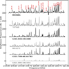Fig. 1

Spectra for six of the sources studied here with the name of each object printed below each spectrum. The molecules associated with several lines are also stated in red next to the lines.

Table 1

Fitted parameters of N-bearing species.

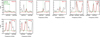Fig. 2

Best model for ${CH}_{3}^{13} CN$ ${\rm{CH}}_{\rm{3}}^{{\rm{13}}}{\rm{CN}}$ of the source 881427C (red), which has narrow lines with FWHM = 5.5 km s⁻¹ on top of the data (black). In this figure only lines with A_ij > 10⁻⁶ s⁻¹ and E_up < 500 K are shown. The detected lines that are mainly considered for the fits are marked with an 'X' on the top right. The dashed line shows the 3σ level.

Fig. 3

Same as Fig. 2 but for source G345.5043+00.3480 with broad lines (FWHM = 7.8 km s⁻¹).

Fig. 4

Summary of the detected species toward the sources. Plus signs show the detected and tentatively detected molecules and minus signs show the non-detections. The sources are ordered from left to right from the lowest to highest distance. The tentative detection of CH₃NH₂ in sources 707948 and 787212 is uncertain due to line blending and more data is needed for a more robust confirmation.

3 Results

3.1 Detection statistics

Figure 4 presents the molecules detected in each of the sources. Plus signs show the (tentatively) detected molecules and minus signs show the non-detected molecules. The sources in this figure are ordered by their distances from the Hi-Gal or RMS surveys (see Table E.3; Lumsden et al. 2013; Mège et al. 2021) where 881427C is the source with the closest distance (1.5 kpc) and G025.6498+01.0491 is the source with the farthest distance (12.20 kpc).

Methanol, methyl cyanide, and isocyanic acid are detected in all sources because the sample is chosen so that the sources are all line-rich. The isotopologues of these species are detected in ≳76% of the sources. Ethyl cyanide and formamide are (tentatively) detected in all sources except one and C₂H₃CN is (tentatively) detected in ~78% of all sources.

From the molecules shown in Fig. 4, CH₃NH₂ is the least (tentatively) detected molecule, in only 12 sources (in ~32% of the sources). This molecule has intrinsically weak lines (A_ij ≲ 5 × 10⁻⁵ s⁻¹; see Table E.7) making it difficult to detect. In fact, it has only been detected toward a handful of high-mass sources in the ISM such as Sgr B2 (Kaifu et al. 1974; Belloche et al. 2013; Neill et al. 2014), Orion KL B (Cernicharo et al. 2016), three cores in NGC 6334I (Bøgelund et al. 2019b), the Galactic Center cloud G+0.693 (Zeng et al. 2018) and the hot core G10.47+0.03 (Ohishi et al. 2019). It is also detected in a spiral galaxy at red-shift 0.89 (Muller et al. 2011). But it was not detected towards the low-mass protostar IRAS 16293-2422B (Ligterink et al. 2018). Therefore, (tentative) detection of this molecule in 12 additional sources is increasing this sample size by more than a factor of 2.

Moreover, as seen from Fig. 4, there are more minus signs toward the right hand side of this figure, that is, for sources located at larger distances. Therefore, the fact that some molecules are not detected in some sources could be the sensitivity limit. However, there is not a clear correlation between luminosity and detection as shown in Fig. D.16.

3.2 Spatial extent

Figure 5 presents the moment zero (integrated intensity) maps of four lines for four of the sources whose spectra are included in Fig. 1. The lines and sources selected are a few examples of the types of sources and line spatial distributions seen in the sample. The transitions with their upper energy levels are printed on each panel of Fig. 5 in white. Moreover, the continuum contours are shown for each source in black.

The high mass clumps considered in this work show complex structures in their dust emission. They often present multiple continuum sources in a single field of view. However, not all the continuum bright regions show emission from the species considered here. Often, only a single source in each region is bright in complex organic emission which is the source that we extract the spectrum from.

The species considered here (a few presented in Fig. 5) usually originate from a single compact region with radii of ~ 1000–7500 au. Therefore, assuming a single T_ex and FWHM for one molecule is valid as long as lines are relatively optically thin.

The emission is mostly unresolved, although it is clear that some lines show more extended emission. For example, the HNCO and C₂H₅ CN transitions presented here show more compact emission compared to CH₃OH and CH₃CN lines. However, these speculations are line dependent as the emission region depends on the upper energy level of the line and its optical depth. Higher spatial resolution data are needed to measure the column densities and excitation temperatures as a function of distance from the central source. Although the emission is usually unresolved, some spatial information can be obtained by looking into the excitation temperatures of various species as discussed in Sect. 4.1.

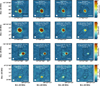Fig. 5

Moment zero maps of four selected lines for four sources included in Fig. 1. The line, name of the source and E_up of the line are printed in white at the middle top of each panel. The beam is also shown on the bottom left of each panel. The continuum contours are shown in black and are at [3, 5, 10, 20, 30]σ_cont with σ_cont for the sources from top to bottom being 7.6, 4.1, 1.9 and 0.8 mJy beam⁻¹, respectively. The scale bars on the bottom right of each panel from top to bottom show lengths of 10942, 7199, 11518, and 39089 au at the distances of the sources.

3.3 Excitation temperatures

It is possible to measure the excitation temperatures of ${CH}_{3}^{18} OH$ ${\rm{CH}}_{\rm{3}}^{{\rm{18}}}{\rm{OH}}$ , ¹³CH₃CN, C₂H₃ CN, HN¹³ CO, NH₂CHO and CH₃NH₂ for at least nine sources. Table 1 presents these values. The excitation temperature of ${CH}_{3}^{18} OH$ ${\rm{CH}}_{\rm{3}}^{{\rm{18}}}{\rm{OH}}$ is likely biased toward lower temperatures given that it is mainly measured from two lines with E_up < 100 K and one transition with E_up = 238.9 K. The latter usually provides a good upper limit on the excitation temperature. Figure 6 shows the average excitation temperatures for these species where measurement of T_ex was possible (see Figs. D.1–D.5 for examples of how excitation temperatures were measured). The error bars in this figure are calculated as follows. For each molecule the average of excitation temperatures, average of their upper (i.e., T_ex + T_err,up) and lower values (i.e., T_ex–T_err,low) for different sources are calculated. Then the error bars show the difference between the upper and lower averages with the mean of the excitation temperatures. The molecules in this figure are ordered by increasing binding energy from left to right.

This figure shows that the species studied here fall in three categories in terms of their excitation temperatures. Cold species (T_ex ≲ 100 K) are found to be ${CH}_{3}^{18} OH$ ${\rm{CH}}_{\rm{3}}^{{\rm{18}}}{\rm{OH}}$ and CH₃NH₂. Warm species (100 K ≲ T_ex ≲ 250 K) are found to be ¹³CH₃CN, HN¹³ CO and C₂H₃CN. NH₂CHO is found to be a hot molecule (T_ex ≳ 250 K).

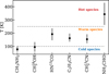Fig. 6

Mean of the excitation temperatures of the species in sources where the temperature is fitted. The error bars are calculated as explained in the text. The species are ordered by their binding energies from low (left) to high (right). The dashed lines are to separate the three groups of species seen.

3.4 Column densities

The fitted column densities of the species investigated here are presented in Tables 1 and E.l. It is important to note that methanol column densities here are found for spectra extracted from the peak of moment zero maps of CH₃CN 12₄–11₄ while the values in van Gelder et al. (2022b) are found from spectra extracted centered at the continuum peak. Moreover, here the temperatures are fitted for ¹⁸O methanol while in van Gelder et al. (2022b) the temperatures were fixed to 150 K. Therefore, variations in column densities of methanol between these two works are expected. These variations are always within a factor ~4 but for most sources they are only within a factor ~2.

Given the large number of sources considered in this work, one can investigate if there is any correlation between the column densities of various species. We do this by using the Pearson's r coefficient. It is calculated by the following equation for our sample in logarithmic space $r_{P} = \frac{\sum_{i} (N_{1, i} - {\bar{N}}_{1}) (N_{2, i} - {\bar{N}}_{2})}{{(\sum_{i} {(N_{1, i} - {\bar{N}}_{1})}^{2} \sum_{i} {(N_{2, i} - {\bar{N}}_{2})}^{2})}^{0.5}},$ ${r_{\rm{P}}} = {{\sum\nolimits_i {\left( {{N_{1,i}} - {{\bar N}_1}} \right)\left( {{N_{2,i}} - {{\bar N}_2}} \right)} } \over {{{\left( {\sum\nolimits_i {{{\left( {{N_{1,i}} - {{\bar N}_1}} \right)}^2}} \sum\nolimits_i {{{\left( {{N_{2,i}} - {{\bar N}_2}} \right)}^2}} } \right)}^{0.5}}}},$ (1)

where N₁ and N₂ are the column densities of the two species that r_P is calculated for, ${\bar{N}}_{1}$ ${\bar N_1}$ and ${\bar{N}}_{2}$ ${\bar N_2}$ are the mean of the column densities of species 1 and 2 and the sums are over the sources in our sample indicated by i.

Figure 7 presents the correlation matrix for the Pearson's r coefficients of the column densities of the studied species. Additionally, Fig. D.17 presents column densities of the species plotted versus each other. It is important to note that sources whose methanol column density is derived from ¹³CH₃OH (instead of ${CH}_{3}^{18} OH$ ${\rm{CH}}_{\rm{3}}^{{\rm{18}}}{\rm{OH}}$ ) are excluded in Fig. 7. This is to eliminate the potential optical depth issues with ¹³CH₃OH. For these sources ${CH}_{3}^{18} OH$ ${\rm{CH}}_{\rm{3}}^{{\rm{18}}}{\rm{OH}}$ was either not detected or the lines were too blended to derive reliable column densities of this molecule (see Sect. 2.2). Figure D.18 presents the same figure but including the sources where methanol column density is found from ¹³CH₃OH and all species except CH₃NH₂ show weaker correlation with methanol. This is likely due to the optical depth effects of ¹³CH₃OH. Figure 7 shows that most species have strong (r_P > 0.7) positive correlations with each other except for CH₃NH₂ that does not show such strong correlation with most other species.

Ethyl cyanide and methyl cyanide are found to have the tightest correlation with r_P of 0.94. In fact, there is a tight correlation (r_P > 0.88) between all three molecules in the cyanide group: CH₃CN, C₂H₃CN and C₂H₅CN. Other observational studies have also seen the strong correlation between CH₃CN and C₂H₅CN. Yang et al. (2021) find r_P = 0.85 for the column density normalized by the continuum brightness of these molecules in the PEACHES sample for low-mass protostars. Moreover, Law et al. (2021) find a correlation coefficient of 0.91 for the column densities of these two molecules in their spatially resolved data of the high-mass star forming region, G10.6-0.4.

It is notable that absolute values of column densities depend on the source size assumed and the amount of warm gas mass in the beam of the observations. Therefore, if a source has more warm mass in the beam all the species are enhanced. Hence, the most interesting fact in Fig. 7 is the weaker correlation of CH₃NH₂ with most species (see Sect. 4.5).

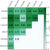Fig. 7

Correlation matrix for Pearson coefficient of the column densities. The darkest green shows the highest correlation. In this figure sources with their methanol column density found from ¹³CH₃OH are excluded due to optical depth effects.

4 Discussion

4.1 Implications of the measured excitation temperatures

Figure 6 shows three categories of species based on their excitation temperatures (see Sect. 3.3). A similar temperature segregation was found toward IRAS 16293-2422B (Jørgensen et al. 2018) and seven high-mass young stellar objects (Bisschop et al. 2007). The differences seen in the excitation temperatures of various molecules can be due to the differences in their desorption temperatures which depends on the binding energies of these species in their respective ice matrix. Taking the binding energies of these species in amorphous solid water, formamide has the highest binding energy (Chaabouni et al. 2018; Ferrero et al. 2020; Minissale et al. 2022) and CH₃NH₂ has the lowest one (Chaabouni et al. 2018) compared with the other species. The rest of the molecules ( ${CH}_{3}^{18} OH$ ${\rm{CH}}_{\rm{3}}^{{\rm{18}}}{\rm{OH}}$ ; HN¹³CO; C₂H₃CN; and ¹³CH₃CN) have similar binding energies in between (Collings et al. 2004; Das et al. 2018; Song & Kästner 2016; Wakelam et al. 2017; Bertin et al. 2017; Penteado et al. 2017; Ferrero et al. 2020; Minissale et al. 2022). Therefore, assuming that the excitation temperature represents the temperature of the environment to some extent, the pattern seen in Fig. 6 is consistent with the pattern seen in binding energies and desorption temperatures of these species.

One can assume that the excitation temperatures of these species give information on the temperature of the environment that these species are tracing. If this is the case NH₂CHO is tracing the hotter regions closer to the protostar, ${CH}_{3}^{18} OH$ ${\rm{CH}}_{\rm{3}}^{{\rm{18}}}{\rm{OH}}$ and CH₃NH₂ trace the cold temperatures farther from the protostar and the rest of the molecules trace regions in between. In other words the pattern seen in the excitation temperatures point to existing of an 'onion-like' structure around the protostar. A similar onion-like structure was also observed around the hot corinos of IRAS 16293-2422 and SVS13-A binary systems (Manigand et al. 2020; Bianchi et al. 2022). This is particularly interesting as it can be an indication of different emitting areas of these species while this information cannot be obtained with the angular resolution of the data used here. In particular the low excitation temperature of ${CH}_{3}^{18} OH$ ${\rm{CH}}_{\rm{3}}^{{\rm{18}}}{\rm{OH}}$ indicates a more extended emission of this molecule compared with some of the other species such as formamide. Although the low E_up lines of ¹²CH₃OH also trace emission from outflows (Tychoniec et al. 2021), in this work we do not use methanol itself but rather its ¹⁸O isotopologue to find the column density of ¹²C-methanol for most sources. Therefore, the ¹²C-methanol column densities should mainly trace the gas in the envelope or disk around the protostar. The implication of different emitting areas on column density measurements and their ratios is discussed in Sect. 4.4.

4.2 NH₂CHO versus HNCO

This section is focused on two molecules whose relationship has been discussed extensively in the literature: NH₂CHO and HNCO. Figure 8 presents the column densities of the two plotted against each other. In the top panel the data points are presented and a simple curve of the form $N_{{NH}_{2} CHO} = 199 \times N_{HNCO}^{0.79}$ ${N_{{\rm{N}}{{\rm{H}}_{\rm{2}}}{\rm{CHO}}}} = 199 \times N_{{\rm{HNCO}}}^{0.79}$ is fitted to the column densities. In the bottom panel, we compare the result of our fit with other studies. Red shows the fit to the column densities of these two molecules towards the high-mass star forming region NGC 6334I (Ligterink et al. 2020). Orange shows the same from Law et al. (2021) for the massive star forming region G10.6-0.4. Blue, pink and black are the fits to the abundances of NH₂CHO and HNCO with respect to $N_{H_{2}}$ ${N_{{{\rm{H}}_2}}}$ from López-Sepulcre et al. (2015), Quénard et al. (2018) and Colzi et al. (2021) normalized by a factor 10^23(1−y), where y is the exponent of the fit to the abundances and N_H2 is assumed to be 10²³ for all (see Appendix B for the explanation of the normalization). Therefore, one can only compare the slopes of the curves shown in the bottom panel of Fig. 8 rather than the absolute values of the column densities. In general, the slopes of the relations between NH₂CHO and HNCO column densities (i.e., the exponents) agree well between the different data sets with the slopes being slightly steeper in the observations of Quénard et al. (2018) and Law et al. (2021).

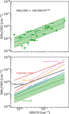Fig. 8

Column density of NH₂CHO versus column density of HNCO. Top panel: data points from the ALMAGAL survey found in this work with the best fit plotted as the middle solid line and the shaded green area showing the 68 percentile scatter in the data. Bottom panel: compares the fitted data in our work by studies from López-Sepulcre et al. (2015), Quénard et al. (2018), Ligterink et al. (2020), Law et al. (2021) and Colzi et al. (2021). The curves for López-Sepulcre et al. (2015), Quénard et al. (2018) and Colzi et al. (2021) are taken from the fit to abundances of NH₂CHO and HNCO and are normalized here as explained in the text: only slopes can be compared, not the absolute values.

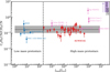Fig. 9

Column density ratio of C₂H₅CN to CH₃CN versus bolometric luminosity for low- and high-mass sources. The red points show the values for ALMAGAL sources from this work. Blue and pink show values for low- and high-mass protostars taken from the literature (see Table E.4 for the references). Moreover, the purple bar shows the range of C₂H₅CN/CH₃CN peak gas-phase values from Garrod et al. (2022) in the warm-up stages with slow, medium and fast pace (from their Table 17, final model setup). The purple arrow shows that the range of models are higher than the range in this plot. Upward triangles show lower limits and downward triangles show upper limits. Grey solid line and shaded gray area show the mean and standard deviation weighted by the uncertainty on the log₁₀ of each column density ratio after eliminating upper and lower limits. Moreover, Sgr B2(N2) is eliminated in the derivation of mean and standard deviation, as it often seems to be an outlier.

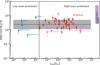Fig. 10

Same as Fig. 9, but for HNCO/CH₃CN. The literature values are taken from studies presented in Table E.4. In this plot SMM1-a is colored blue although it is an intermediate mass protostar.

4.3 Going from low- to high-mass protostars

The absolute values of column densities discussed in Sects. 3.4 and 4.2 are not as informative as column density ratios because the former are dependent on the beam size which is not the same in all sources. The column density ratios are not dependent on the beam size, but they are dependent on the emitting areas of the two species in the ratio. This effect needs to be considered and is explained in depth in Sect. 4.4.2. However, in this Section we consider the column density ratios and the general trends seen for them.

Figures 9, 10 and 11 present the column density ratios of C₂H₅CN to CH₃CN, HNCO to CH₃CN and NH₂CHO to CH₃OH for the sources studied in this work as well as other low- and high-mass protostars from the literature. Appendix D presents the same figures for some additional combination of species. Each plot covers four orders of magnitude in ratio. The solid black line in each figure shows the mean of the (log₁₀) column density ratios. The shaded-gray regions indicate the 1σ scatter of the (log₁₀) column density ratios around this mean value. The means and standard deviations include the data from this work and the literature, for low- and high-mass protostars, and are weighted by the errors on each data point. Moreover, the upper limits, lower limits and the Sgr B2(N2) source are excluded from this calculation. The 1er scatter values in log space (i.e., dex) can be converted to a 'factor of spread' around the mean value as 10^dex. These factors are summarized in Table and are shown in Fig. 12.

It is important to note that the calculated scatter for the low-mass protostars are mainly based on a select number (four or five) of measurements available from the literature. Therefore, one cannot make any conclusions solely based on the calculated scatter in low-mass protostars. The PEACHES survey that studies ~50 low-mass protostars does not include HNCO, and with their relatively short integration times ¹⁸O methanol iso-topologue lines are unfortunately not detected for most of their sources. Moreover, the column density of CH₃CN is found from the main isotopologue lines which are likely optically thick. Hence, their column density values are not included in the quantification of the scatter.

The scatter in column density ratios of all sources, as shown in Fig. 12, is less than a factor of about three. In other words they are remarkably constant. Given the sensitivity of COM abundances to temperature and time (Garrod 2013; Garrod et al. 2022; Aikawa et al. 2020), these constant ratios imply that the physical conditions in which the complex organics are formed are similar (see e.g., Quénard et al. 2018; Coletta et al. 2020; Belloche et al. 2020). Hence, our data indicate that COMs are formed during the phase of star formation in which the physical conditions are mainly constant and similar for all species. The studied hot cores, span a range of orders of magnitude in luminosities (see Table E.3). This means that the hot core stage of the various ALMAGAL sources should have large differences in gas temperature and radiation field. Therefore, the most likely phase in which the physical conditions are mainly constant is that of the cold cloud prior to collapse, that is, the pre-stellar phase during which most molecules are frozen out and formation of complex molecules in ices can take place. Another possibility is that the precursors of these species are formed in the pre-stellar ices while COMs form later in the gas in a manner that the column density ratios stay constant. Given that this latter argument adds an extra level of complexity (i.e., needing constant physical conditions in the pre-stellar phase and the protostellar phase), the former argument, where COMs are likely forming in the pre-stellar ices, could be a more probable interpretation.

In Fig. 12 the C₂H₅CN/CH₃CN column density ratio has the lowest scatter compared to other species combinations. In fact there is only a factor of 1.66 spread around the mean for C₂H₅CN/CH₃CN in all sources. The spread factor is in general small (≲2) for all ratios that relate the species in the cyanide group with each other. The scatter increases for other ratios presented in Fig. 12. For instance, all ratios that include NH₂CHO have a large spread factor, with most having a scatter larger than a factor 2.5 around the mean. Moreover, the ratios that include CH₃NH₂, on average, show higher spread factors compared to the ratios that do not include this molecule or NH₂CHO. These trends are also seen in Fig. 7. It should be noted that the number of sources with CH₃NH₂ detection is lower than that of the other species studied here, and therefore, the conclusions made here should be confirmed with more data points in the future.

The remaining species show spread factors ≲2 5 (Table 2). In general, this is a small scatter given the range of envelope masses (~1–5000 M_⊙) and luminosities (~2−10⁷ L_⊙) of the sources studied here, all scattered across various regions in the sky. However, there are some differences in the spread factors of various column density ratios in Fig. 12. The reason for such differences in the spread factor can be either physical or chemical. The physical and chemical effects are discussed in Sects. 4.4 and 4.5.

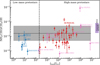Fig. 11

Same as Fig. 9, but for NH₂CHO/CH₃OH. The red hollow circles indicate the sources for which ¹³CH₃OH was used to find the column density of CH₃OH.

Table 2

Factor of spread around the mean defined as 10^dex.

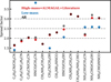Fig. 12

One σ scatter around the mean of log₁₀ of the column density ratios. Both mean and standard deviation are weighted by the errors on each data point. Blue shows the values for low-mass protostars where there were more than two sources available for this calculation. Red shows the scatter for high-mass protostars and black presents those for all sources available (i.e., low- and high-mass protostars).

4.4 Physical effects

4.4.1 Optical depth

First, optical depth of the lines can be an issue when calculating the column density ratios and their scatter. This is especially an important problem for abundant species and those with bright lines such as HNCO, CH₃CN, CH₃OH and often NH₂CHO. Therefore, the column densities of these species could be underestimated in some sources because all their lines are potentially optically thick.

In this work the values for the column densities of HNCO, CH₃CN and CH₃OH are found from the column densities of their less abundant isotopologues as an attempt to solve the problem of optical depth. However, lines originating from the isotopologues can also become optically thick for very line-rich sources. The modeled optical depths of the HN¹³CO lines toward the most line-rich source, 707948, are less than 0.1. Moreover, H¹⁵NCO is not detected toward any of our sources. For 707 948, HN¹³CO/H¹⁵NCO is ≳0.4 compared with the ¹³C/¹⁵N isotopo-logue ratio of ~7. Although these limits are not enough to prove that HN¹³CO is optically thin but it can be an indication that optical depth might not be a major problem for HN¹³CO. It is also less likely that ${CH}_{3}^{18} OH$ ${\rm{CH}}_{\rm{3}}^{{\rm{18}}}{\rm{OH}}$ lines are optically thick but for the sources where ¹³CH₃OH is used to obtain the column densities of CH₃OH (indicated by a star in Table E.1), optical depth can be an issue. These sources are shown as hollow red circles in Fig. 11 for the ratio of NH₂CHO/CH₃OH. The column density ratios of the three ALMAGAL sources with luminosities >3 × 10⁴ L_⊙ are on the higher end suggesting that the methanol column density is likely underestimated due to optical thickness of ${CH}_{3}^{18} OH$ ${\rm{CH}}_{\rm{3}}^{{\rm{18}}}{\rm{OH}}$ lines. These are indeed the three line rich sources (101899, 707948 and G343.1261-00.0623) for which due to extreme line blending it was not possible to find the column density of ${CH}_{3}^{18} OH$ ${\rm{CH}}_{\rm{3}}^{{\rm{18}}}{\rm{OH}}$ and hence ¹³CH₃OH was used. Moreover, it is possible that for the most line-rich sources some of ${CH}_{3}^{18} OH$ ${\rm{CH}}_{\rm{3}}^{{\rm{13}}}{\rm{CN}}$ lines start becoming optically thick but for most such sources this problem is mitigated by finding the column density from the CH₃CN 12₁₀−11₁₀ line if it is less optically thick than the ${CH}_{3}^{18} OH$ ${\rm{CH}}_{\rm{3}}^{{\rm{13}}}{\rm{CN}}$ lines. Finally, the column densities found for NH₂CHO can suffer from line optical depth issues as was found in NGC 6334I (Ligterink et al. 2020). However, ${NH}_{2}^{13} CHO$ ${\rm{NH}}_2^{13}{\rm{CHO}}$ was not detected for some of the most line rich sources in this work. The 3σ upper limits of ${NH}_{2}^{13} CHO$ ${\rm{NH}}_2^{13}{\rm{CHO}}$ can be converted to NH₂CHO upper limits using ¹²C/¹³C ratios in Table E.3. These values obtained for NH₂CHO are indeed larger than the measured column density of formamide as expected and result in more optically thick lines of NH₂CHO (while over producing the lines). For some of the most line-rich sources (e.g., 707948) the low E_up line of formamide becomes marginally optically thick (τ ≃ 0.1) if a beam dilution factor of 2 is assumed. Therefore, the column densities of NH₂CHO for most line-rich sources should be taken with care.

Considering other values presented in Figs. 9–11 from the literature, similar issues hold when calculating the column densities. The column densities from the literature are chosen carefully so this problem is minimized. However, as an example S68N in Fig. 9 is a data point with large error bars and falls above the main spread. This is because the lines are weak in S68N and none of the isotopologues of CH₃CN except its deuterated versions are detected (Nazari et al. 2021). Moreover, the values of HNCO, CH₃CN and CH₃OH in G10.6 cores may be suffering from optical depth problems as explained carefully in Law et al. (2021). The HNCO column densities for IRAS 16293 A and B can also be suffering from line optical thickness issues. This is because HNCO value for IRAS 16293 A was found from the main isotopologue of this molecule (Manigand et al. 2020) and in IRAS 16293 B except HN¹³CO other isotopologues of HNCO such as DNCO are also detected (Coutens et al. 2016) indicating that even HN¹³CO might be optically thick. However, in general it is safe to assume that for most sources shown here (especially the ALMAGAL data) line optical depth is unlikely to have a large effect.

Dust optical depth can also have an effect on the column density ratios. It is true that the dust will affect all species coming from the same region to the same extent. However, if the species considered have different emitting areas, dust optical depth can affect the species closer to the protostar more and alter the column density ratios. This is especially evident in source 693050 as discussed by van Gelder et al. (2022b) where the methanol emission is seen in a ring shaped structure around the continuum emission. Given Fig. 6 and as discussed in Sect. 4.1, NH₂CHO should be tracing the closest regions to the protostar. Therefore, the effect of dust opacity should be the largest for the ratios including formamide. From these ratios NH₂CHO/HNCO is notable as many studies have found a correlation between these two species (see Sect. 4.2). But Fig. 12 shows that the spread factor calculated for this ratio is one of the largest when compared with the other ratios considered here. One of the main reasons of this high spread is potentially the larger effect of dust opacity on NH₂CHO.

4.4.2 Source structure

The second physical effect on column density ratios is the difference in emitting areas of the two species in a ratio. The column density found from an emitting region is directly proportional to the area of the emission. In this study the area of the emission is assumed to be the same for all species in a source. However, due to variations in sublimation temperatures some species can trace hotter regions closer to the protostar as seen for NH₂CHO in Fig. 6 and some species can trace colder regions further from the protostar as seen for ${CH}_{3}^{18} OH$ ${\rm{CH}}_{\rm{3}}^{{\rm{18}}}{\rm{OH}}$ in the same figure. Therefore, the assumption that the emitting area of these two species are the same is not correct. Nazari et al. (2021) show that for a toy model of a spherically symmetric envelope with power law structure in density and temperature (their Sect. 4.3 and Appendix B) the ratio of column densities for two molecules is related to the ratio of their abundances by $\frac{N_{1}}{N_{2}} = \frac{X_{1}}{X_{2}} {(\frac{T_{1, sub}}{T_{2, sub}})}^{- 3.75},$ ${{{N_1}} \over {{N_2}}} = {{{X_1}} \over {{X_2}}}{\left( {{{{T_{1,{\rm{sub}}}}} \over {{T_{2,{\rm{sub}}}}}}} \right)^{ - 3.75}},$ (2)

where X is the abundance with respect to hydrogen and T_sub is the sublimation temperature of a molecule. This means that in order to determine the true abundance ratio for NH₂CHO and CH₃OH which have different sublimation temperatures, a constant factor needs to be multiplied to all the data points in Fig. 11.

This constant factor can be the ratio of their average T_ex found in Fig. 6 or the ratio of their sublimation temperatures from the lab experiments as proposed by Nazari et al. (2021). This will not change the spread seen in this figure, it only moves all the data points by a factor ${(\frac{T_{{CH}_{3} OH,sub}}{T_{{NH}_{2} CHO,sub}})}^{- 3.75}$ ${\left( {{{{T_{{\rm{C}}{{\rm{H}}_{\rm{3}}}{\rm{OH,sub}}}}} \over {{T_{{\rm{N}}{{\rm{H}}_{\rm{2}}}{\rm{CHO,sub}}}}}}} \right)^{ - 3.75}}$ if sublimation temperatures are assumed as in Eq. (2). However, is the assumption that these sources are spherically symmetric (i.e., with no source structure such as disks) valid for all sources considered here?

van Gelder et al. (2022b) find a scatter of ~4 orders of magnitude in warm methanol mass if both line-rich and line-poor sources are included. It is important to note that methanol is known to be a molecule that forms only in the ice and then sublimates into the gas. They explain the reason for the ~4 orders of magnitude scatter based on non-chemical effects including a discussion on the possible existence of disks. When considering the line-rich sources the scatter in van Gelder et al. 2022b becomes only ~2 orders of magnitude which points to the fact that for line-rich sources the effect of a disk is not as considerable. However, ~2 orders of magnitude scatter in methanol mass is still large enough that existence of (smaller) disks are needed to explain all of the spread in methanol mass. Therefore, in the line-rich sample analyzed here not all sources can be assumed as spherically symmetric and may host disks with various (perhaps small) sizes.

Now the question becomes: If a source has a disk, will the ratio of emitting areas of NH₂CHO and CH₃OH stay constant compared with when there is no disk present? It is true that the ratio of sublimation temperatures remains constant but the temperature structure depends on the source structure as seen in the work of Nazari et al. (2022) on low-mass protostars. Figure 13 shows a cartoon of possible emitting areas of NH₂CHO and CH₃OH for a case where a disk is present and a case where it is not. An analogue to Eq. (2) for a case where a disk is present is $\frac{N_{1}}{N_{2}} = \frac{X_{1}}{X_{2}} \frac{f (R_{1, sub, z_{1},sub})}{f (R_{2, sub, z_{2},sub})},$ ${{{N_1}} \over {{N_2}}} = {{{X_1}} \over {{X_2}}}{{f\left( {{R_{1,{\rm{sub,}}{z_1}{\rm{,sub}}}}} \right)} \over {f\left( {{R_{2,{\rm{sub,}}{z_2}{\rm{,sub}}}}} \right)}},$ (3)

where f(R, z) is a function for the emitting area of a species which is dependent on both radius (R) and height (z). The exact shape of this function is not easy to find analytically as the dependence of fon the disk radius cannot be simply written as a power-law relation (see Nazari et al. 2022). Therefore, the ratio of the two functions across various sources is not necessarily constant.

A more quantitative understanding can be achieved by taking the mid-plane temperature in the fiducial envelope-only and envelope plus disk models of Nazari et al. (2022) for an 8 L_⊙ source, and calculate the emitting radius of NH₂CHO and CH₃OH in the mid-plane by assuming the mean excitation temperatures found in Fig. 6 (i.e., ~100 K for methanol and ~300 K for formamide). These are given by 5.1 and 28.6 au for NH₂CHO and CH₃OH in the envelope-only model and by 1.6 au and 5.7 au in the envelope plus disk model. Given that area is proportional to radius squared one can calculate the factor (ratio of the two area functions) in Eq. (3) assuming NH₂CHO being species one and CH₃OH species two as 0.032 for the envelope-only model and 0.079 for the envelope plus disk model. There is a factor 2.5 difference between the two multiplication factors calculated that can alter the ratio of NH₂CHO/CH₃OH for the less line-rich sources. However, this is only a rough approximation by taking the mid-plane temperature. Radiative transfer models are needed for more quantitative understanding of the effect of source structure on the ratios in both low- and high-mass protostars and its effect on chemical implication of the spread. This is beyond the scope of this paper and is considered in other works (see Nazari et al., in prep.).

Finally, the discussion above shows that the effect of dust optical depth and a first order approximation of the disk effect are the highest for ratios including NH₂CHO given its largest excitation temperature among all the species considered here. Therefore, to explain the larger scatter seen in ratios including NH₂CHO in Fig. 12, first one needs to correct for the physical and non-chemical effects.

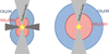Fig. 13

Cartoon of two sources: one with disk (left) and one without (right). The red and blue regions show the emitting regions of NH₂CHO and CH₃OH, respectively. There is not a priory reason as to why the ratio of the two sublimation regions between the two sources should remain constant.

4.5 Chemical implications

4.5.1 Comparison with chemical models

In this section we compare our findings with the existing Garrod et al. (2022) chemical models for protostars. The models discussed in Garrod et al. (2022) build on the models in Garrod (2013, also see Garrod et al. 2008) altering and updating various chemical processes in different steps. Their models go through two physical stages. Collapse, where the gas temperature is kept at 10 K but the density increases and warm-up, where the density is kept constant to the final density in the previous stage (2 × 10⁸ cm⁻³) and temperature increases to 400 K with three different speeds.

The purple bar in figures that present column density ratios (e.g., Figs. 9–11) show the peak gas-phase abundances from Garrod et al. (2022) models in the second stage with variations in the warm-up speed. Starting with C₂H₅CN/CH₃CN, Fig. 9 shows that the 'final' model setup of Garrod et al. (2022) does not agree well with the observations. To dive deeper into these models, Fig. D.29 shows our observational ratios overplotted with their values for different models during the warm-up stage with medium speed (the same plot for C₂H₃CN/CH₃CN has a similar trend). It is seen that the models agree best with the observations where gas-phase chemistry routes (the model on the left of the final model) are not added. They find that for their 'final' model CH₃CN first forms to some extent in the ice but at later stages gas-phase chemistry takes over and most of its production occurs at later stages. Moreover, they find that C₂H₅CN and C₂H₃CN mainly form in ices. However, given that the 'final' model does not agree well with the observational data (more than one order of magnitude difference) could mean that either not enough CH₃CN is produced in the cold stages, too much C₂H₅CN is produced, it is not as effectively destroyed at later hot stages or gas-phase production of CH₃CN is not observed.

The observed column density ratios including CH₃NH₂ mostly differ with the Garrod et al. (2022) models (see purple bar in Figs. D.23–D.25). Figure D.30 shows the comparison of various models in Garrod et al. (2022) with the spread in the data. It is more clear from this figure that most models in Garrod et al. (2022) overproduce CH₃NH₂ assuming that their methanol abundances are more accurate.

Figure D.31 shows the comparison of models with our results for HNCO/CH₃OH. In general the models do a good job (except the two models where they turn off diffusion in the ice mantles) at explaining the data. If the net rate of production of these two species in their final model are compared (their Figs. 13 and 14) much of the HNCO and CH₃OH form at temperatures below 10 K in ices supporting the argument that HNCO and CH₃OH could be forming in the dense core phase.

4.5.2 Observed scatter

One of the key findings of this paper is the relatively small scatter in column density ratios. However, a second finding is that this scatter, while usually small, shows some variations from species to species. This in turn may hold clues on the chemistry and the physical conditions where these molecules are formed. In Appendix C, we develop a simple toy model to explain the scatter of abundance ratios around the mean value (i.e., spread factor, discussed in Sect. 4.3 and presented in Fig. 12) from a chemical point of view. To minimize the contribution from the physical structure and dust optical depth on the scatter of abundance ratios around the mean, we only consider the molecules CH₃OH, CH₃CN, C₂H₅CN, C₂H₃CN, HNCO and CH₃NH₂ (i.e., all except formamide; see Sect. 4.4).

The abundance of a molecule is primarily determined by the environmental conditions (temperature, density, and UV radiation) as well as the amount of time a source has spent in those conditions (Lee et al. 2003; Sakai & Yamamoto 2013). A cloud experiences various stages before forming a main sequence star, each of which are characterized by a distinct set of environmental variables. The bulk of most complex organic species is thought to form in the pre-stellar stage (Herbst & van Dishoeck 2009). Moreover, as discussed in Sect. 4.3, the almost constant column density ratios (spread ≲3) point to formation of these species in similar physical conditions, likely the pre-stellar ices. Hence, we focus on pre-stellar stage in this section.

We determine the abundances in the pre-stellar ices with a toy model, inspired by the available chemical models. Most importantly, we assume that the abundance of each molecule is a function of time (Lee et al. 2003; Aikawa et al. 2020; Garrod et al. 2022). The details of the toy model are given in Appendix C. Equations (C.2) and (C.3) can be used to find $\frac{X_{1, 2}}{\bar{X_{1, 2}}} = {(t / \bar{t})}^{α_{1} - α_{2}} .$ ${{{X_{1,2}}} \over {\overline {{X_{1,2}}} }} = {\left( {t/\bar t} \right)^{{\alpha _1} - {\alpha _2}}}.$ (4)

This is a particularly interesting relation because it clearly shows that the scatter in column density ratios (assumed to be the same as abundance ratios; $X_{1, 2} / \bar{X_{1, 2}}$ ${X_{1,2}}/\overline {{X_{1,2}}}$ can be explained by the scatter in pre-stellar timescales $(t / \bar{t})$ $\left( {t/\bar t} \right)$ without a direct dependence on the exact values of parameters A₁ and A₂ (the ice abundance of each species at 10⁶ yr). In other words, Eq. (4) shows that the scatter in the pre-stellar timescales is the only parameter driving the scatter in abundance ratios (for a given temperature and density condition). Therefore, the distribution of the pre-stellar timescales can be inferred from the distributions of abundance ratios.

Figure 14 presents the scatter in the pre-stellar timescales $(t / \bar{t})$ $\left( {t/\bar t} \right)$ for low- and high-mass protostars. This figure shows that the scatter in column density ratios of some species can be explained by a factor ~ 1, 5–2 spread in the pre-stellar timescales of the low-and high-mass protostars. It is reassuring that the spread in the pre-stellar timescales is approximately constant and independent from the ratio used to find this spread. The small variation in the spreads seen in Fig. 14 is expected. This is because all the scatter seen in the column density ratios (Fig. 12) is not purely due to the variations in pre-stellar timescales but also physical effects explained in Sect. 4.4. It is important to add that these are all based on a simple toy model. Therefore, the exact values for the spread in pre-stellar times or the column density ratios that have a strong correlation with time might change. However, the general idea that the scatter in column density ratios can be (at least partially) explained by the scatter in pre-stellar timescales stays valid regardless of the toy model used. For example if the ice abundances in the ‘static phase’ models of Aikawa et al. (2020) are taken (see their Figs. 3 and 5), a similar toy model can be constructed with a similar trend seen in Fig. D.32. The result would again be that the scatter in abundance ratios can be related to the scatter in pre-stellar lifetimes. As Aikawa et al. (2020) conclude, the variations in COM abundances (mainly O-bearing species in their work) are less than one order of magnitude when the pre-stellar lifetimes are changed. This is consistent with our observations and toy model as we only observe spread factors ≲3.

The implication of such parametrization could be important. For all species, the mean column density ratio inferred from the low-mass sample is roughly similar to the value inferred from the high-mass sample (see Table E.5). Knowing $\bar{X_{1, 2}}$ $\overline {{X_{1,2}}}$ , one can estimate $\bar{t}$ $\bar t$ in Eq. (C.3) for all low- and high-mass protostars. Therefore, given that $\bar{X_{1, 2}}$ $\overline {{X_{1,2}}}$ is the same for low- and high-mass protostars the average duration of pre-stellar phase ( $(\bar{t})$ $\left( {\bar t} \right)$ ) is similar for the low- and high-mass protostars. This is only valid if the other parameters determining the abundances other than time (i.e., α₁, α₂ and A_1,2) are constant. Therefore, the general consensus that high-mass stars have a more rapid pre-main sequence evolution compared to the low-mass stars (e.g., see Davies et al. 2011; Mottram et al. 2011) implies that this faster evolution only occurs after the pre-stellar phase (i.e, warm-up and protostellar phase onward). Hence, pre-stellar phases of low- and high-mass protostars should be similar (pre-stellar lifetimes within factor ~2–3): cold low-mass clouds that can interact to form the high-mass protostars. This implication is in line with the non-detection of high-mass pre-stellar cores suggesting that such high-mass pre-stellar cores simply do not exist (Motte et al. 2018). Moreover, this conclusion agrees with the findings of Pitts et al. (2022) who show that low- and high-mass protostars are statistically indistinguishable on larger envelope scales. Because of the sparsity of the sample of low-mass protostars with such detailed chemistry analyses with ALMA, robust conclusions based on the low-mass sample remain pending increased sample size.

It is also important to mention that the argument above assumes that the temperatures of the pre-stellar environments are constant at ~10 K for both low- and high-mass protostars. In addition, it assumes that the densities increase from ~10³ to ~10⁸ cm⁻³ during the collapse phase. However, if these temperature and densities change (also see Aikawa et al. 2020), the point at which the abundances of these species stop their rapid growth (which is ~10⁵ yr with the assumptions of Garrod et al. 2022 models) can also change to shorter or longer timescales. In other words, the other parameters that the abundance depends on (i.e., A and α) can be dependent on the temperature and density of the pre-stellar phase of each source. Therefore, changes in temperatures and densities can also affect the scatter seen in column density ratios. Finally, we emphasize that these conclusions are based on a simple toy model and for more robust conclusions further study is needed.

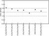Fig. 14

Factor of spread around the mean of the pre-stellar timescales for various low- and high-mass protostars using the spread factor found for low-mass, ALMAGAL and high-mass literature sources (see black points in Fig. 12).

5 Conclusions

We analyzed the spectra of 37 line-rich MYSOs from the ALMAGAL survey. This work focuses on the study of six N-bearing species: CH₃CN, HNCO, NH₂CHO, C₂H₅CN, C₂H₃CN and CH₃NH₂. Our main conclusions are as follows:

Methyl cyanide and isocyanic acid are detected in all the sources selected for this study, whereas ${NH}_{2}^{13} CHO$ ${\rm{NH}}_2^{13}{\rm{CHO}}$ and HN¹³CO are (tentatively) detected in >76% of the sources. Ethyl cyanide and formamide are (tentatively) detected in all sources except one and C₂H₃CN in ~78% of all sources. Methylamine is (tentatively) detected in 12 of the objects in our sample which more than doubles the number of sources with CH₃NH₂ detection in the ISM.
Three groups of species are observed based on their excitation temperatures (Fig. 6). Formamide falls under the hot category (T_ex ≳ 250 K), HN¹³CO, ${NH}_{2}^{13} CHO$ ${\rm{NH}}_2^{13}{\rm{CHO}}$ and C₂H₃CN fall under the warm category (100 K ≲ T_ex ≲ 250 K) and ${CH}_{3}^{18} OH$ ${\rm{CH}}_{\rm{3}}^{{\rm{18}}}{\rm{OH}}$ and CH₃NH₂ fall under the cold category (T_ex ≲ 100 K). The reason for these different groups can mainly be associated with the sublimation temperatures of these molecules.
Assuming excitation temperatures indicate the temperature of the environment in which the species reside, the hot species trace regions closer to the protostar, the cold species trace regions far from the protostar and the warm species trace the regions in between.
Column density ratios of the species studied here are remarkably constant across low- and high-mass protostars (with scatter less than ~3) indicating that these species and/or their precursors form in similar physical environments, most plausibly in pre-stellar ices.
The scatter in column density ratios varies with C₂H₅CN/CH₃CN showing the smallest scatter (spread factor = 1.66) and ratios including formamide and methylamine showing the largest scatter (Fig. 12). Given that formamide is most probably tracing the closest regions to the protostars compared with the other species studied here, the column density ratios including NH₂CHO are most affected by source structure and dust optical depth. Therefore, the scatter in its column density ratios mostly have a physical origin. Source structure and dust optical depth effects are smaller for the ratios including the other molecules and hence are likely not the main origin of the observed scatter.
Assuming that the bulk of complex organics form in the pre-stellar ices, the scatter in the column density ratios could be readily explained by the differences in the time that various clouds spend in the pre-stellar phase in addition to the variations in temperature and density of this phase. If the scatter mainly depends on the time spent in the pre-stellar phase, the data show similar pre-stellar lifetimes for low- and high-mass protostars (within factors of ~2–3).

More robust conclusions can be made by increasing the number of low-mass protostars with such chemistry analysis observed by ALMA. However, with the current data available, the abundances are similar toward low- and high-mass protostars indicating that these species form in similar pre-stellar physical conditions.

Acknowledgements

We would like to thank the referee for very constructive comments. We also thank R. T. Garrod for providing us with some of their model outputs. Astrochemistry in Leiden is supported by the Netherlands Research School for Astronomy (NOVA), by funding from the European Research Council (ERC) under the European Union’s Horizon 2020 research and innovation programme (grant agreement No. 101019751 MOLDISK), and by the Dutch Research Council (NWO) grants 618.000.001, TOP-1 614.001.751, and 648.000.022. Support by the Danish National Research Foundation through the Center of Excellence “InterCat” (Grant agreement no.: DNRF150) is also acknowledged. This paper makes use of the following ALMA data: ADS/JAO.ALMA#2019.1.00195.L. ALMA is a partnership of ESO (representing its member states), NSF (USA) and NINS (Japan), together with NRC (Canada), MOST and ASIAA (Taiwan), and KASI (Republic of Korea), in cooperation with the Republic of Chile. The Joint ALMA Observatory is operated by ESO, AUI/NRAO and NAOJ. The National Radio Astronomy Observatory is a facility of the National Science Foundation operated under cooperative agreement by Associated Universities, Inc. D.L. was supported by a grant from VILLUM FONDEN (project number 16599). N.F.W.L. acknowledges funding by the Swiss National Science Foundation (SNSF) Ambizione grant 193453. B.T. is a Laureate of the Paris Region fellowship program, which is supported by the Ile-de-France Region and has received funding under the Horizon 2020 innovation framework program and Marie Sklodowska-Curie grant agreement No. 945298.

Appendix A Spectroscopic data

The line list and the respective spectroscopic data for CH₃CN and ${CH}_{2}^{13} CN$ ${\rm{NH}}_2^{13}{\rm{CHO}}$ are taken from the JPL database (Kukolich et al. 1973; Boucher et al. 1977; Demaison et al. 1979; Kukolich 1982; Anttila et al. 1993; Pearson & Mueller 1996; Cazzoli & Puzzarini 2006; Müller et al. 2009). The vibration factor can be assumed to be similar for CH₃CN and ${CH}_{3}^{13} CN$ ${\rm{CH}}_{\rm{3}}^{{\rm{18}}}{\rm{OH}}$ at the excitation temperatures found in this work. The vibration factor for CH₃CN is less than 1.1 for temperatures below 180 K (Müller et al. 2015) and hence are ignored in this paper.

The line list for C₂H₅CN is taken from the CDMS (Mäder et al. 1974; Johnson et al. 1977; Boucher et al. 1980; Pearson et al. 1994; Fukuyama et al. 1996). The vibrational correction factor for this molecule is between ~1.1 and ~2.1 for the temperatures assumed here (Heise et al. 1981). For temperatures below 120 K we have assumed no vibrational correction factor as it is negligible. For sources with assumed excitation temperature 120K ≤ T_ex ≤ 140 K we use a vibrational correction factor of 1.3174, if T_ex = 150 K a correction factor of 1.3848 is used, if T_ex is 160 K or 170 K we use 1.4591, if T_ex = 200 K a correction factor of 1.8316 is used and finally when T_ex = 220 K we use 2.1318.

For C₂H₃CN the spectroscopic data are taken from the CDMS (Gerry & Winnewisser 1973; Stolze & Sutter 1985; Cazzoli & Kisiel 1988; Demaison et al. 1994; Baskakov et al. 1996; Colmont et al. 1997; Müller et al. 2008). Low lying vibrational modes are included in its partition function. The line lists for HNCO and its isotopologues are taken from the JPL database (Hocking et al. 1975; Pickett et al. 1998).

NH₂CHO v=0 and NH₂CHO v₁2=1 entries are taken from the CDMS (Kukolich & Nelson 1971; Hirota et al. 1974; Moskienko & Dyubko 1991; Vorob’eva & Dyubko 1994; Kryvda et al. 2009; Motiyenko et al. 2012). For all the sources a vibrational correction factor of 1.5 for 300K is used. CH₃NH₂ spectroscopic data were taken from the JPL database (Ilyushin et al. 2005; Kréglewski & Wlodarczak 1992; Kręglewski et al. 1992; Ohashi et al. 1987; Takagi & Kojima 1971; Nishikawa 1957; Shimoda et al. 1954). Methanol line list is taken from the CDMS database (Lees & Baker 1968; Pickett et al. 1981; Xu et al. 2008).

Appendix B Normalization in Figure 8

Figure 8 shows the absolute values of column densities of different works in its bottom panel. However, not all the works from the literature present their fitted lines to the absolute values of column densities but they show the fit to the abundances of the two molecules NH₂CHO and HNCO. Therefore, to use their fits in Fig. 8 one needs to use a method to convert a fit to the abundances to a fit to column densities. Here this method is explained.

The fit to the column densities can be written as: $N_{{NH}_{2} CHO} = x^{'} \times N_{HNCO}^{y^{'}},$ ${N_{{\rm{N}}{{\rm{H}}_{\rm{2}}}{\rm{CHO}}}} = x' \times N_{{\rm{HNCO}}}^{y'},$ (B.1)

and the fit to the abundances can be written as: $N_{{NH}_{2} CHO} / N_{H} = x \times {(\frac{N_{HNCO}}{N_{H}})}^{y} .$ ${N_{{\rm{N}}{{\rm{H}}_{\rm{2}}}{\rm{CHO}}}}/{N_{\rm{H}}} = x \times {\left( {{{{N_{{\rm{HNCO}}}}} \over {{N_{\rm{H}}}}}} \right)^y}.$ (B.2)

By rearranging Eq. (B.2) $N_{{NH}_{2} CHO} = x N_{H} / N_{H}^{y} \times N_{HNCO}^{y} .$ ${N_{{\rm{N}}{{\rm{H}}_{\rm{2}}}{\rm{CHO}}}} = x{N_{\rm{H}}}/N_{\rm{H}}^y \times N_{{\rm{HNCO}}}^y.$ (B.3)

Therefore, by comparing Equations (B.1) and (B.3) one can see that y = y′ and hence the slopes of the two fits can be compared. However, $x^{'} = x N_{H}^{1 - y}$ $x' = xN_{\rm{H}}^{1 - y}$ and thus a value for the column density of Hydrogen is needed. Here we assume an N_H = 10²³ for simplicity to normalize all the values from different works.

Appendix C Chemical toy model

We define the pre-stellar phase to be as when the cloud is becoming more centrally concentrated and the densities increase while the temperatures remain low (~10 K). This is the phase during which the extinction, A_v, increases from ~1 – 2 (i.e., translucent cloud; Snow & McCall 2006) to ≳9, the CO freeze-out takes place (Boogert et al. 2015), and is similar to the ‘collapse stage’ in chemical models of Garrod et al. (2022). Based on the abundances calculated in the collapse stage of Garrod et al. (2022) models (their Fig. 9), they increase rapidly in the first < 10⁵ yr of the collapse and then increase with a shallower slope from 10⁵ yr to 10⁶ yr. Given that the pre-stellar phase of star formation usually lasts around 10⁵ yr and 10⁶ yr (supported by the values found from water and CO observations; Schmalzl et al. 2014; Jørgensen et al. 2005), we particularly focus on molecular abundances between ~10⁵ and ~10⁶ years in our toy model. Therefore, we define the abundance, X_i, of species i with respect to hydrogen as $X_{i} = A_{i} {(\frac{t}{10^{6} yr})}^{α_{i}},$ ${X_{\rm{i}}} = {A_{\rm{i}}}{\left( {{t \over {{{10}^6}{\rm{yr}}}}} \right)^{{\alpha _i}}},$ (C.1)

where A_i is the ice abundance of each molecule after 10⁶ years, t is the duration of the pre-stellar phase and α_i is a positive unique constant for each molecule.

We approximate the ice abundance of each molecule at 10⁶ yr, A_i, using the ice abundance of each species at the end of the collapse stage of Garrod et al. (2022) models. These models are only used as an inspiration for the parametrization and are only an example of the chemical models available in the literature. The same can be done with other chemical models of the pre-stellar phase in the literature. Moreover, α_i can be estimated using the ice abundances at 10⁵ yr and 10⁶ yr in Fig. 9 of Garrod et al. (2022) for each molecule. Therefore, Eq. (C.1) gives the abundance of each species (in solids) between 10⁵ yr and 10⁶ yr into the collapse (typical age for the pre-stellar phase). The assumed α_i are given in Table E.6 and the resulting abundances are plotted in Fig. D.32. It is important to note that, as explained in Sect. 4.5.1, the Garrod et al. (2022) models likely underestimate the ice abundance of CH₃CN. Therefore, in our toy model we assume a larger $A_{{CH}_{3} CN}$ ${A_{{\rm{C}}{{\rm{H}}_{\rm{3}}}{\rm{CN}}}}$ to be consistent with observations. The same is done for CH₃NH₂, where the models likely overestimate the abundance of this molecule in ices (see Sect. 4.5.1).

Using Eq. (C.1) we can find the abundance ratios (assumed to be the same as column density ratios) of two species 1 and 2 as $X_{1,2} = A_{1,2} {(\frac{t}{10^{6}})}^{α_{1} - α_{2}} .$ ${X_{{\rm{1,2}}}} = {A_{{\rm{1,2}}}}{\left( {{t \over {{{10}^6}}}} \right)^{{\alpha _1} - {\alpha _2}}}.$ (C.2)

Here X₁/X₂ and A₁/A₂ are written as X_1,2 and A_1,2 respectively. If the left hand side of Eq. (C.2) is the mean of the observed abundance ratios ( $(\bar{X_{1, 2}})$ $\left( {\overline {{X_{1,2}}} } \right)$ ), t on the right hand side corresponds to the average time that various clouds spend in the pre-stellar phase ( $\bar{t}$ $\bar t$ ); in other words: $\bar{X_{1,2}} = A_{1,2} {(\frac{\bar{t}}{10^{6}})}^{α_{1} - α_{2}} .$ $\overline {{X_{{\rm{1,2}}}}} = {A_{{\rm{1,2}}}}{\left( {{{\bar t} \over {{{10}^6}}}} \right)^{{\alpha _1} - {\alpha _2}}}.$ (C.3)

This equation can be used to replace A_1,2 in Eq. (C.2), to give Eq. (4) in the main text. If α₁ ≃ α₂, the correlation between X_1,2 and t would be weak, making them degenerate. Hence, it will not be possible to infer t from X_1,2 confidently. This is true for the ratios of C₂H₃CN/CH₃CN and HNCO/CH₃CN where α₁ – α₂ is 0.3 and 0.2 respectively (see Table E.6). However, since this is not the case for other ratios in Fig. 12 (i.e., α₁ ≠ α₂), the distribution of the pre-stellar timescales can be inferred from the distributions of abundance ratios (see Fig. 14).

Appendix D Additional plots

Figures D.1–D.5 show how the excitation temperature was measured for an example source 767784 and species NH₂CHO, ${CH}_{3}^{18} OH$ ${\rm{CH}}_{\rm{3}}^{{\rm{18}}}{\rm{OH}}$ and CH₃NH₂. Figures D.6–D.15 show the best-fit models of the N-bearing species considered in this work for two example sources 881427 (narrow lines) and G345.5043+00.3480 (broad lines).

Figure D.16 presents what molecule is (tentatively) detected (plus signs) and what molecule is not detected (minus signs) in each source where the sources are ordered by increasing luminosity from left to right. Figure D.17 presents the column density of the species considered here versus each other with the Pearson’s r printed on the top left of each plot. Figure D.18 is the same as Fig. 7 but including the sources where methanol column density was measured from its (potentially optically thick) ¹³C isotopologue. Figures D.19–D.28 show column density ratios of various species with respect to each other versus luminosity for the ALMAGAL sources in addition to the literature sources. The values for literature sources are taken from the references given in Table E.4.

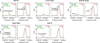Fig. D.1

Demonstration of how excitation temperature upper and lower bounds are determined for NH₂CHO for source 767784. The various symbols are the same as Fig. 2.

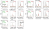Fig. D.2

Demonstration of how excitation temperature upper and lower bounds are determined for ${CH}_{3}^{18} OH$ ${\rm{CH}}_{\rm{3}}^{{\rm{18}}}{\rm{OH}}$ for source 767784. The various symbols are the same as Fig. 2.

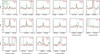Fig. D.3

Showing that excitation temperature of 60 K does not match the observations for CH₃NH₂ in source 767784. The various symbols are the same as Fig. 2. Here a few lines are overestimated, for example, the ones with E_up of 17.3 K and 92.2 K and if the column density is decreased lines such as the ones with E_up of 156.5 K and 182.1 K will be underestimated.

Fig. D.4

Best-fit model for CH₃NH₂ in source 767784. The various symbols are the same as Fig. 2.

Figures D.29–D.31 present the column density ratios calculated from Table 15 of Garrod et al. (2022) that show the peak gas phase abundances of a few N-bearing species during the warm-up phase of their chemical models with medium pace warm-up. These plots also show the scatter seen in the data for both low-and high-mass protostars found in this work. Figure D.32 shows the abundances of the species considered here calculated with the toy model as a function of time spent in the pre-stellar phase.

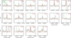Fig. D.5

Showing that excitation temperature of 150 K does not match the observations for CH₃NH₂ in source 767784. The various symbols are the same as Fig. 2. Again here some lines are overestimated and if the column density is decreased the lines that are perfect fits now will be underestimated.

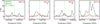Fig. D.6

Best model for HN¹³CO of source 881427 (red) on top of the data (black). In this figure only lines with A_ij > 10⁻⁶ s⁻¹ and E_up < 700 K are shown. Moreover, only one representative plot of the hyper fine structure of this molecule is shown to avoid repetition. The detected lines that are mainly considered for the fits are marked with an ‘X’ on the top right. The dashed lines shows the 3σ line.

Fig. D.7

Same as Fig. D.6, but for G345.5043+00.3480.

Fig. D.8

Same as Fig. D.6, but for C₂H₅CN.

Fig. D.9

Same as Fig. D.6, but for G345.5043+00.3480 and C₂H₅CN.

Fig. D.10

Same as Fig. D.6, but for C₂H₃CN.

Fig. D.11

Same as Fig. D.6, but for G345.5043+00.3480 and C₂H₃CN.

Fig. D.12

Same as Fig. D.6, but for CH₃NH₂.

Fig. D.13

Same as Fig. D.6, but for G345.5043+00.3480 and CH₃NH₂.

Fig. D.14

Same as Fig. D.6, but for NH₂CHO. Here only lines with A_ij > 10⁻⁵ s⁻¹ are shown.

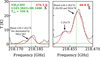Fig. D.15

Same as Fig. D.6, but for G345.5043+00.3480 and NH₂CHO. Here only lines with A_ij > 10⁻⁵ s⁻¹ are shown.

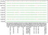Fig. D.16

Same as Fig. 4, but now the sources are ordered from left to right from the lowest to highest luminosity.

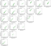Fig. D.17

Correlations seen in column densities. Column densities of the molecules considered in this work plotted versus each other. Only detected molecules are plotted here. The Pearson’s r coefficient is given at the top left of each panel.

Fig. D.18

Same as Fig. 7, but column densities of methanol found from ¹³CH₃OH are also included.

Fig. D.19

Same as Fig. 9, but for C₂H₃CN/C₂H₅CN. The references are given in Table E.4.

Fig. D.20

Same as Fig. 9, but for C₂H₃CN/CH₃CN. The references are given in Table E.4.

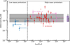Fig. D.21

Same as Fig. 9, but for HNCO/CH₃OH. In this plot SMM1-a is colored blue although it is an intermediate mass protostar. The references are given in Table E.4. The red hollow circles indicate the sources for which ¹³CH₃OH was used to find the column density of CH₃OH.

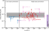Fig. D.22

Same as Fig. 9, but for CH₃CN/CH₃OH. In this plot SMM1-a is colored blue although it is an intermediate mass protostar. The references are given in Table E.4. The red hollow circles indicate the sources for which ¹³CH₃OH was used to find the column density of CH₃OH.

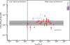Fig. D.23

Same as Fig. 9, but for CH₃NH₂/CH₃OH. The references are given in Table E.4. The red hollow circles indicate the sources for which ¹³CH₃OH was used to find the column density of CH₃OH.

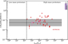Fig. D.24

Same as Fig. 9, but for CH₃NH₂/HNCO. The references are given in Table E.4. The luminosity for source G+0.693 is assumed at 10⁴ as no estimation of the luminosity was found for this source.

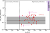Fig. D.25

Same as Fig. 9, but for CH₃NH₂/CH₃CN. The references are given in Table E.4. The luminosity for source G+0.693 is assumed at 10⁴ as no estimation of the luminosity was found for this source.

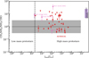Fig. D.26

Same as Fig. 9, but for CH₃NH₂/NH₂CHO. The references are given in Table E.4. The luminosity for source G+0.693 is assumed at 10⁴ as no estimation of the luminosity was found for this source.

Fig. D.27

Same as Fig. 9, but for NH₂CHO/CH₃CN. The references are given in Table E.4.

Fig. D.28

Same as Fig. 9, but for NH₂CHO/HNCO. The references are given in Table E.4.

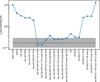Fig. D.29

Spread highlighted in Fig. 9 (gray) is over plotted with values from Table 15 of Garrod et al. (2022) that show the peak gas phase abundances of a few N-bearing species during their warm up phase (blue).

Fig. D.30

Same as Fig. D.29, but for CH₃NH₂/CH₃OH.

Fig. D.31

Same as Fig. D.29, but for HNCO/CH₃OH.

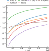Fig. D.32

Abundances assumed for the toy model.

Appendix E Additional Tables

Table E.1

Fitted parameters for methanol.

Table E.2

Observational parameters for each source.

Table E.3

Source properties from the Hi-GAL survey.

Table E.4

The references for column densities used in the column density ratio plots and the calculation of the scatter.

Table E.5

Weighted averages

Table E.6

Assumed values for α.

Table E.7

All transitions of the N-bearing species studied here in the data that have E_up < 1000 K.

References

Aikawa, Y., Furuya, K., Yamamoto, S., & Sakai, N. 2020, ApJ, 897, 110 [Google Scholar]
Anttila, R., Horneman, V. M., Koivusaari, M., & Paso, R. 1993, J. Mol. Spectr., 157, 198 [Google Scholar]
Barone, V., Latouche, C., Skouteris, D., et al. 2015, MNRAS, 453, L31 [Google Scholar]
Baskakov, O. I., Dyubko, S. F., Ilyushin, V. V., et al. 1996, J. Mol. Spectr., 179, 94 [NASA ADS] [CrossRef] [Google Scholar]
Belloche, A., Müller, H. S. P., Menten, K. M., Schilke, P., & Comito, C. 2013, A&A, 559, A47 [NASA ADS] [CrossRef] [EDP Sciences] [Google Scholar]
Belloche, A., Müller, H. S. P., Garrod, R. T., & Menten, K. M. 2016, A&A, 587, A91 [NASA ADS] [CrossRef] [EDP Sciences] [Google Scholar]
Belloche, A., Meshcheryakov, A. A., Garrod, R. T., et al. 2017, A&A, 601, A49 [NASA ADS] [CrossRef] [EDP Sciences] [Google Scholar]
Belloche, A., Maury, A. J., Maret, S., et al. 2020, A&A, 635, A198 [NASA ADS] [CrossRef] [EDP Sciences] [Google Scholar]
Beltrán, M. T., Codella, C., Viti, S., Neri, R., & Cesaroni, R. 2009, ApJ, 690, L93 [Google Scholar]
Bertin, M., Doronin, M., Fillion, J. H., et al. 2017, A&A, 598, A18 [NASA ADS] [CrossRef] [EDP Sciences] [Google Scholar]
Bianchi, E., López-Sepulcre, A., Ceccarelli, C., et al. 2022, ApJ, 928, L3 [NASA ADS] [CrossRef] [Google Scholar]
Bisschop, S. E., Jørgensen, J. K., van Dishoeck, E. F., & de Wachter, E. B. M. 2007, A&A, 465, 913 [NASA ADS] [CrossRef] [EDP Sciences] [Google Scholar]
Bisschop, S. E., Jørgensen, J. K., Bourke, T. L., Bottinelli, S., & van Dishoeck, E. F. 2008, A&A, 488, 959 [NASA ADS] [CrossRef] [EDP Sciences] [Google Scholar]
Blake, G. A., Sutton, E. C., Masson, C. R., & Phillips, T. G. 1987, ApJ, 315, 621 [Google Scholar]
Bøgelund, E. G., McGuire, B. A., Ligterink, N. F. W., et al. 2018, A&A, 615, A88 [Google Scholar]
Bøgelund, E. G., Barr, A. G., Taquet, V., et al. 2019a, A&A, 628, A2 [NASA ADS] [CrossRef] [EDP Sciences] [Google Scholar]
Bøgelund, E. G., McGuire, B. A., Hogerheijde, M. R., van Dishoeck, E. F., & Ligterink, N. F. W. 2019b, A&A, 624, A82 [EDP Sciences] [Google Scholar]
Boogert, A. C. A., Pontoppidan, K. M., Knez, C., et al. 2008, ApJ, 678, 985 [Google Scholar]
Boogert, A. C. A., Gerakines, P. A., & Whittet, D. C. B. 2015, ARA&A, 53, 541 [Google Scholar]
Bottinelli, S., Ceccarelli, C., Lefloch, B., et al. 2004, ApJ, 615, 354 [Google Scholar]
Boucher, D., Burie, J., Demaison, J., et al. 1977, J. Mol. Spectr., 64, 290 [NASA ADS] [CrossRef] [Google Scholar]
Boucher, D., Dubrulle, A., Demaison, J., & Dreizler, H. 1980, Z. Nat. Teil A, 35, 1136 [NASA ADS] [Google Scholar]
Bulak, M., Paardekooper, D. M., Fedoseev, G., & Linnartz, H. 2021, A&A, 647, A82 [NASA ADS] [CrossRef] [EDP Sciences] [Google Scholar]
Calcutt, H., Jørgensen, J. K., Müller, H. S. P., et al. 2018, A&A, 616, A90 [NASA ADS] [CrossRef] [EDP Sciences] [Google Scholar]
Cazaux, S., Tielens, A. G. G. M., Ceccarelli, C., et al. 2003, ApJ, 593, L51 [NASA ADS] [CrossRef] [Google Scholar]
Cazzoli, G., & Kisiel, Z. 1988, J. Mol. Spectr., 130, 303 [NASA ADS] [CrossRef] [Google Scholar]
Cazzoli, G., & Puzzarini, C. 2006, J. Mol. Spectr., 240, 153 [NASA ADS] [CrossRef] [Google Scholar]
Cernicharo, J., Kisiel, Z., Tercero, B., et al. 2016, A&A, 587, L4 [NASA ADS] [CrossRef] [EDP Sciences] [Google Scholar]
Chaabouni, H., Diana, S., Nguyen, T., & Dulieu, F. 2018, A&A, 612, A47 [NASA ADS] [CrossRef] [EDP Sciences] [Google Scholar]
Chuang, K. J., Fedoseev, G., Scirè, C., et al. 2021, A&A, 650, A85 [NASA ADS] [CrossRef] [EDP Sciences] [Google Scholar]
Codella, C., Ceccarelli, C., Caselli, P., et al. 2017, A&A, 605, L3 [NASA ADS] [CrossRef] [EDP Sciences] [Google Scholar]
Coletta, A., Fontani, F., Rivilla, V. M., et al. 2020, A&A, 641, A54 [NASA ADS] [CrossRef] [EDP Sciences] [Google Scholar]
Collings, M. P., Anderson, M. A., Chen, R., et al. 2004, MNRAS, 354, 1133 [NASA ADS] [CrossRef] [Google Scholar]
Colmont, J. M., Wlodarczak, G., Priem, D., et al. 1997, J. Mol. Spectr., 181, 330 [NASA ADS] [CrossRef] [Google Scholar]
Colzi, L., Rivilla, V. M., Beltrán, M. T., et al. 2021, A&A, 653, A129 [NASA ADS] [CrossRef] [EDP Sciences] [Google Scholar]
Coutens, A., Jørgensen, J. K., van der Wiel, M. H. D., et al. 2016, A&A, 590, L6 [NASA ADS] [CrossRef] [EDP Sciences] [Google Scholar]
Das, A., Sil, M., Gorai, P., Chakrabarti, S. K., & Loison, J. C. 2018, ApJS, 237, 9 [NASA ADS] [CrossRef] [Google Scholar]
Davies, B., Hoare, M. G., Lumsden, S. L., et al. 2011, MNRAS, 416, 972 [Google Scholar]
Demaison, J., Dubrulle, A., Boucher, D., Burie, J., & Typke, V. 1979, J. Mol. Spectr., 76, 1 [NASA ADS] [CrossRef] [Google Scholar]
Demaison, J., Cosleou, J., Bocquet, R., & Lesarri, A. G. 1994, J. Mol. Spectr., 167, 400 [NASA ADS] [CrossRef] [Google Scholar]
Dulieu, F., Nguyen, T., Congiu, E., Baouche, S., & Taquet, V. 2019, MNRAS, 484, L119 [NASA ADS] [CrossRef] [Google Scholar]
Elia, D., Molinari, S., Schisano, E., et al. 2017, MNRAS, 471, 100 [NASA ADS] [CrossRef] [Google Scholar]
Elia, D., Merello, M., Molinari, S., et al. 2021, MNRAS, 504, 2742 [NASA ADS] [CrossRef] [Google Scholar]
Fedoseev, G., Chuang, K. J., van Dishoeck, E. F., Ioppolo, S., & Linnartz, H. 2016, MNRAS, 460, 4297 [Google Scholar]
Fedoseev, G., Chuang, K. J., Ioppolo, S., et al. 2017, ApJ, 842, 52 [Google Scholar]
Ferrero, S., Zamirri, L., Ceccarelli, C., et al. 2020, ApJ, 904, 11 [NASA ADS] [CrossRef] [Google Scholar]
Fontani, F., Pascucci, I., Caselli, P., et al. 2007, A&A, 470, 639 [NASA ADS] [CrossRef] [EDP Sciences] [Google Scholar]
Förstel, M., Bergantini, A., Maksyutenko, P., Góbi, S., & Kaiser, R. I. 2017, ApJ, 845, 83 [Google Scholar]
Fuchs, G. W., Cuppen, H. M., Ioppolo, S., et al. 2009, A&A, 505, 629 [NASA ADS] [CrossRef] [EDP Sciences] [Google Scholar]
Fukuyama, Y., Odashima, H., Takagi, K., & Tsunekawa, S. 1996, ApJS, 104, 329 [NASA ADS] [CrossRef] [Google Scholar]
Garrod, R. T. 2013, ApJ, 765, 60 [Google Scholar]
Garrod, R. T., Widicus Weaver, S. L., & Herbst, E. 2008, ApJ, 682, 283 [Google Scholar]
Garrod, R. T., Belloche, A., Müller, H. S. P., & Menten, K. M. 2017, A&A, 601, A48 [NASA ADS] [CrossRef] [EDP Sciences] [Google Scholar]
Garrod, R. T., Jin, M., Matis, K. A., et al. 2022, ApJS, 259, 1 [NASA ADS] [CrossRef] [Google Scholar]
Gerry, M. C. L., & Winnewisser, G. 1973, J. Mol. Spectr., 48, 1 [NASA ADS] [CrossRef] [Google Scholar]
Gibb, E., Nummelin, A., Irvine, W. M., Whittet, D. C. B., & Bergman, P. 2000, ApJ, 545, 309 [NASA ADS] [CrossRef] [Google Scholar]
Gorai, P., Bhat, B., Sil, M., et al. 2020, ApJ, 895, 86 [Google Scholar]
Gorai, P., Das, A., Shimonishi, T., et al. 2021, ApJ, 907, 108 [NASA ADS] [CrossRef] [Google Scholar]
Grim, R. J. A., & Greenberg, J. M. 1987, ApJ, 321, L91 [NASA ADS] [CrossRef] [Google Scholar]
Grim, R. J. A., Baas, F., Geballe, T. R., Greenberg, J. M., & Schutte, W. A. 1991, A&A, 243, 473 [NASA ADS] [Google Scholar]
Haupa, K. A., Tarczay, G., & Lee, Y.-P. 2019, J. Am. Chem. Soc., 141, 11614 [CrossRef] [Google Scholar]
Heise, H. M., Winther, F., & Lutz, H. 1981, J. Mol. Spectr., 90, 531 [NASA ADS] [CrossRef] [Google Scholar]
Herbst, E., & van Dishoeck, E. F. 2009, ARA&A, 47, 427 [NASA ADS] [CrossRef] [Google Scholar]
Hirota, E., Sugisaki, R., Nielsen, C. J., & Sørensen, G. O. 1974, J. Mol. Spectr., 49, 251 [NASA ADS] [CrossRef] [Google Scholar]
Hocking, W. H., Gerry, M. C. L., & Winnewisser, G. 1975, Canadian J. Phys., 53, 1869 [NASA ADS] [CrossRef] [Google Scholar]
Honma, M., Nagayama, T., & Sakai, N. 2015, PASJ, 67, 70 [NASA ADS] [CrossRef] [Google Scholar]
Hsu, S.-Y., Liu, S.-Y., Liu, T., et al. 2022, ApJ, 927, 218 [NASA ADS] [CrossRef] [Google Scholar]
Hudson, R. L., & Moore, M. H. 2004, Icarus, 172, 466 [Google Scholar]
Ilyushin, V. V., Alekseev, E. A., Dyubko, S. F., Motiyenko, R. A., & Hougen, J. T. 2005, J. Mol. Spectr., 229, 170 [NASA ADS] [CrossRef] [Google Scholar]
Jaber, A. A., Ceccarelli, C., Kahane, C., & Caux, E. 2014, ApJ, 791, 29 [Google Scholar]
Jacobsen, S. K., Jørgensen, J. K., Di Francesco, J., et al. 2019, A&A, 629, A29 [NASA ADS] [CrossRef] [EDP Sciences] [Google Scholar]
Johnson, D. R., Lovas, F. J., Gottlieb, C. A., et al. 1977, ApJ, 218, 370 [NASA ADS] [CrossRef] [Google Scholar]
Jones, B. M., Bennett, C. J., & Kaiser, R. I. 2011, ApJ, 734, 78 [Google Scholar]
Jørgensen, J. K., Schöier, F. L., & van Dishoeck, E. F. 2005, A&A, 435, 177 [NASA ADS] [CrossRef] [EDP Sciences] [Google Scholar]
Jørgensen, J. K., van der Wiel, M. H. D., Coutens, A., et al. 2016, A&A, 595, A117 [Google Scholar]
Jørgensen, J. K., Müller, H. S. P., Calcutt, H., et al. 2018, A&A, 620, A170 [Google Scholar]
Kahane, C., Ceccarelli, C., Faure, A., & Caux, E. 2013, ApJ, 763, L38 [CrossRef] [Google Scholar]
Kaifu, N., Morimoto, M., Nagane, K., et al. 1974, ApJ, 191, L135 [Google Scholar]
Kim, Y. S., & Kaiser, R. I. 2011, ApJ, 729, 68 [NASA ADS] [CrossRef] [Google Scholar]
Kréglewski, M., & Wlodarczak, G. 1992, J. Mol. Spectr., 156, 383 [CrossRef] [Google Scholar]
Kręglewski, M., Stahl, W., Grabow, J.-U., & Wlodarczak, G. 1992, Chem. Phys. Lett., 196, 155 [CrossRef] [Google Scholar]
Kryvda, A. V., Gerasimov, V. G., Dyubko, S. F., Alekseev, E. A., & Motiyenko, R. A. 2009, J. Mol. Spectr., 254, 28 [NASA ADS] [CrossRef] [Google Scholar]
Kukolich, S. G. 1982, J. Chem. Phys., 76, 97 [NASA ADS] [CrossRef] [Google Scholar]
Kukolich, S. G., & Nelson, A. C. 1971, Chem. Phys. Lett., 11, 383 [NASA ADS] [CrossRef] [Google Scholar]
Kukolich, S. G., Ruben, D. J., Wang, J. H. S., & Williams, J. R. 1973, J. Chem. Phys., 58, 3155 [NASA ADS] [CrossRef] [Google Scholar]
Law, C. J., Zhang, Q., Öberg, K. I., et al. 2021, ApJ, 909, 214 [Google Scholar]
Lee, J.-E., Evans, Neal J.I., Shirley, Y. L., & Tatematsu, K. 2003, ApJ, 583, 789 [NASA ADS] [CrossRef] [Google Scholar]
Lee, C.-F., Codella, C., Li, Z.-Y., & Liu, S.-Y. 2019, ApJ, 876, 63 [Google Scholar]
Lees, R. M., & Baker, J. G. 1968, J. Chem. Phys., 48, 5299 [NASA ADS] [CrossRef] [Google Scholar]
Ligterink, N. F. W., Coutens, A., Kofman, V., et al. 2017, MNRAS, 469, 2219 [Google Scholar]
Ligterink, N. F. W., Calcutt, H., Coutens, A., et al. 2018, A&A, 619, A28 [NASA ADS] [CrossRef] [EDP Sciences] [Google Scholar]
Ligterink, N. F. W., El-Abd, S. J., Brogan, C. L., et al. 2020, ApJ, 901, 37 [Google Scholar]
Ligterink, N. F. W., Ahmadi, A., Coutens, A., et al. 2021, A&A, 647, A87 [NASA ADS] [CrossRef] [EDP Sciences] [Google Scholar]
López-Sepulcre, A., Jaber, A. A., Mendoza, E., et al. 2015, MNRAS, 449, 2438 [CrossRef] [Google Scholar]
López-Sepulcre, A., Sakai, N., Neri, R., et al. 2017, A&A, 606, A121 [NASA ADS] [CrossRef] [EDP Sciences] [Google Scholar]
López-Sepulcre, A., Balucani, N., Ceccarelli, C., et al. 2019, ACS Earth Space Chem., 3, 2122 [CrossRef] [Google Scholar]
Lumsden, S. L., Hoare, M. G., Urquhart, J. S., et al. 2013, ApJS, 208, 11 [Google Scholar]
Mäder, H., Heise, H. M., & Dreizler, H. 1974, Z. Nat. Teil A, 29, 164 [Google Scholar]
Manigand, S., Jørgensen, J. K., Calcutt, H., et al. 2020, A&A, 635, A48 [NASA ADS] [CrossRef] [EDP Sciences] [Google Scholar]
Martín-Doménech, R., Öberg, K. I., & Rajappan, M. 2020, ApJ, 894, 98 [Google Scholar]
McGuire, B. A. 2022, ApJ Supplement Series, 259, 30 [NASA ADS] [CrossRef] [Google Scholar]
McMullin, J. P., Waters, B., Schiebel, D., Young, W., & Golap, K. 2007, ASP Conf. Ser., 376, 127 [Google Scholar]
Mège, P., Russeil, D., Zavagno, A., et al. 2021, A&A, 646, A74 [NASA ADS] [CrossRef] [EDP Sciences] [Google Scholar]
Milam, S. N., Savage, C., Brewster, M. A., Ziurys, L. M., & Wyckoff, S. 2005, ApJ, 634, 1126 [Google Scholar]
Minissale, M., Aikawa, Y., Bergin, E., et al. 2022, ACS Earth Space Chem., 6, 597 [NASA ADS] [CrossRef] [Google Scholar]
Molet, J., Brouillet, N., Nony, T., et al. 2019, A&A, 626, A132 [EDP Sciences] [Google Scholar]
Molinari, S., Swinyard, B., Bally, J., et al. 2010, A&A, 518, L100 [NASA ADS] [CrossRef] [EDP Sciences] [Google Scholar]
Moskienko, E. M., & Dyubko, S. F. 1991, Radiophys. Quant. Electron., 34, 181 [NASA ADS] [CrossRef] [Google Scholar]
Motiyenko, R. A., Tercero, B., Cernicharo, J., & Margulès, L. 2012, A&A, 548, A71 [NASA ADS] [CrossRef] [EDP Sciences] [Google Scholar]
Motte, F., Bontemps, S., & Louvet, F. 2018, ARA&A, 56, 41 [NASA ADS] [CrossRef] [Google Scholar]
Mottram, J. C., Hoare, M. G., Davies, B., et al. 2011, ApJ, 730, L33 [Google Scholar]
Müller, H. S. P., Thorwirth, S., Roth, D. A., & Winnewisser, G. 2001, A&A, 370, L49 [Google Scholar]
Müller, H. S. P., Schlöder, F., Stutzki, J., & Winnewisser, G. 2005, J. Mol. Struc., 742, 215 [Google Scholar]
Müller, H. S. P., Belloche, A., Menten, K. M., Comito, C., & Schilke, P. 2008, J. Mol. Spectr., 251, 319 [Google Scholar]
Müller, H. S. P., Drouin, B. J., & Pearson, J. C. 2009, A&A, 506, 1487 [NASA ADS] [CrossRef] [EDP Sciences] [Google Scholar]
Muller, S., Beelen, A., Guélin, M., et al. 2011, A&A, 535, A103 [NASA ADS] [CrossRef] [EDP Sciences] [Google Scholar]
Müller, H. S. P., Brown, L. R., Drouin, B. J., et al. 2015, J. Mol. Spectr., 312, 22 [CrossRef] [Google Scholar]
Nazari, P., van Gelder, M. L., van Dishoeck, E. F., et al. 2021, A&A, 650, A150 [EDP Sciences] [Google Scholar]
Nazari, P., Tabone, B., Rosotti, G. P., et al. 2022, A&A, 663, A58 [NASA ADS] [CrossRef] [EDP Sciences] [Google Scholar]
Neill, J. L., Bergin, E. A., Lis, D. C., et al. 2014, ApJ, 789, 8 [Google Scholar]
Nishikawa, T. 1957, J. Phys. Soc. Japan, 12, 668 [NASA ADS] [CrossRef] [Google Scholar]
Öberg, K. I., Garrod, R. T., van Dishoeck, E. F., & Linnartz, H. 2009, A&A, 504, 891 [NASA ADS] [CrossRef] [EDP Sciences] [Google Scholar]
Öberg, K. I., Boogert, A. C. A., Pontoppidan, K. M., et al. 2011, ApJ, 740, 109 [Google Scholar]
Ohashi, N., Takagi, K., Hougen, J. T., Olson, W. B., & Lafferty, W. J. 1987, J. Mol. Spectr., 126, 443 [Google Scholar]
Ohishi, M., Suzuki, T., Hirota, T., Saito, M., & Kaifu, N. 2019, PASJ, 71, 86 [NASA ADS] [CrossRef] [Google Scholar]
Pearson, J. C., & Mueller, H. S. P. 1996, ApJ, 471, 1067 [NASA ADS] [CrossRef] [Google Scholar]
Pearson, J. C., Sastry, K. V. L. N., Herbst, E., & De Lucia, F. C. 1994, ApJS, 93, 589 [Google Scholar]
Penteado, E. M., Walsh, C., & Cuppen, H. M. 2017, ApJ, 844, 71 [Google Scholar]
Pickett, H. M., Cohen, E. A., Brinza, D. E., & Schaefer, M. M. 1981, J. Mol. Spectr., 89, 542 [NASA ADS] [CrossRef] [Google Scholar]
Pickett, H. M., Poynter, R. L., Cohen, E. A., et al. 1998, J. Quant. Spectr Rad. Transf., 60, 883 [NASA ADS] [CrossRef] [Google Scholar]
Pitts, R. L., Kristensen, L. E., Jørgensen, J. K., & van der Walt, S. J. 2022, A&A, 657, A70 [NASA ADS] [CrossRef] [EDP Sciences] [Google Scholar]
Qasim, D., Fedoseev, G., Chuang, K. J., et al. 2019, A&A, 627, A1 [NASA ADS] [CrossRef] [EDP Sciences] [Google Scholar]
Quénard, D., Jiménez-Serra, I., Viti, S., Holdship, J., & Coutens, A. 2018, MNRAS, 474, 2796 [Google Scholar]
Raunier, S., Chiavassa, T., Duvernay, F., et al. 2004, A&A, 416, 165 [NASA ADS] [CrossRef] [EDP Sciences] [Google Scholar]
Rimola, A., Skouteris, D., Balucani, N., et al. 2018, ACS Earth Space Chem., 2, 720 [Google Scholar]
Rivilla, V. M., Beltrán, M. T., Cesaroni, R., et al. 2017, A&A, 598, A59 [NASA ADS] [CrossRef] [EDP Sciences] [Google Scholar]
Sakai, N., & Yamamoto, S. 2013, Chem. Rev., 113, 8981 [Google Scholar]
Schilke, P., Groesbeck, T. D., Blake, G. A., & Phillips, T. G. 1997, ApJS, 108, 301 [NASA ADS] [CrossRef] [Google Scholar]
Schmalzl, M., Visser, R., Walsh, C., et al. 2014, A&A, 572, A81 [NASA ADS] [CrossRef] [EDP Sciences] [Google Scholar]
Shimoda, K., Nishikawa, T., & Itoh, T. 1954, J. Phys. Soc. Japan, 9, 974 [NASA ADS] [CrossRef] [Google Scholar]
Skouteris, D., Vazart, F., Ceccarelli, C., et al. 2017, MNRAS, 468, L1 [NASA ADS] [Google Scholar]
Snow, T. P., & McCall, B. J. 2006, ARA&A, 44, 367 [NASA ADS] [CrossRef] [Google Scholar]
Song, L., & Kästner, J. 2016, Phys. Chem. Chem. Phys., 18, 29278 [NASA ADS] [CrossRef] [Google Scholar]
Stolze, M., & Sutter, D. H. 1985, Z. Natur. Teil A, 40, 998 [NASA ADS] [CrossRef] [Google Scholar]
Taban, I. M., Schutte, W. A., Pontoppidan, K. M., & van Dishoeck, E. F. 2003, A&A, 399, 169 [NASA ADS] [CrossRef] [EDP Sciences] [Google Scholar]
Takagi, K., & Kojima, T. 1971, J. Phys. Soc. Japan, 30, 1145 [NASA ADS] [CrossRef] [Google Scholar]
Taniguchi, K., Guzmán, A. E., Majumdar, L., Saito, M., & Tokuda, K. 2020, ApJ, 898, 54 [Google Scholar]
Theulé, P., Duvernay, F., Danger, G., et al. 2013, Adv. Space Res., 52, 1567 [CrossRef] [Google Scholar]
Turner, B. E. 1991, ApJS, 76, 617 [NASA ADS] [CrossRef] [Google Scholar]
Tychoniec, Ł., van Dishoeck, E. F., van’t Hoff, M. L. R., et al. 2021, A&A, 655, A65 [NASA ADS] [CrossRef] [EDP Sciences] [Google Scholar]
van Broekhuizen, F. A., Keane, J. V., & Schutte, W. A. 2004, A&A, 415, 425 [NASA ADS] [CrossRef] [EDP Sciences] [Google Scholar]
van Broekhuizen, F. A., Pontoppidan, K. M., Fraser, H. J., & van Dishoeck, E. F. 2005, A&A, 441, 249 [NASA ADS] [CrossRef] [EDP Sciences] [Google Scholar]
van Dishoeck, E. F., Blake, G. A., Jansen, D. J., & Groesbeck, T. D. 1995, ApJ, 447, 760 [Google Scholar]
van Gelder, M. L., Tabone, B., Tychoniec, Ł., et al. 2020, A&A, 639, A87 [NASA ADS] [CrossRef] [EDP Sciences] [Google Scholar]
van Gelder, M. L., Jaspers, J., Nazari, P., et al. 2022a, A&A, 667, A136 [NASA ADS] [CrossRef] [EDP Sciences] [Google Scholar]
van Gelder, M. L., Nazari, P., Tabone, B., et al. 2022b, A&A, 662, A67 [NASA ADS] [CrossRef] [EDP Sciences] [Google Scholar]
van’t Hoff, M. L. R., Harsono, D., Tobin, J. J., et al. 2020, ApJ, 901, 166 [Google Scholar]
Vastel, C., Bottinelli, S., Caux, E., Glorian, J. M., & Boiziot, M. 2015, in SF2A-2015: Proceedings of the Annual meeting of the French Society of Astronomy and Astrophysics, 313 [Google Scholar]
Vorob’eva, E. M., & Dyubko, S. F. 1994, Radiophys. Quant. Electron., 37, 155 [Google Scholar]
Wakelam, V., Loison, J. C., Mereau, R., & Ruaud, M. 2017, Mol. Astrophys., 6, 22 [NASA ADS] [CrossRef] [Google Scholar]
Williams, G. M., Cyganowski, C. J., Brogan, C. L., et al. 2022, MNRAS, 509, 748 [Google Scholar]
Wilson, T. L., & Rood, R. 1994, ARA&A, 32, 191 [Google Scholar]
Xu, L.-H., Fisher, J., Lees, R. M., et al. 2008, J. Mol. Spectr., 251, 305 [NASA ADS] [CrossRef] [Google Scholar]
Yang, Y.-L., Sakai, N., Zhang, Y., et al. 2021, ApJ, 910, 20 [Google Scholar]
Zeng, S., Jiménez-Serra, I., Rivilla, V. M., et al. 2018, MNRAS, 478, 2962 [Google Scholar]
Zeng, S., Jiménez-Serra, I., Rivilla, V. M., et al. 2021, ApJ, 920, L27 [NASA ADS] [CrossRef] [Google Scholar]

¹

http://cassis.irap.omp.eu/

All Tables

Table 1

Fitted parameters of N-bearing species.

In the text

Table 2

Factor of spread around the mean defined as 10^dex.

In the text

Table E.1

Fitted parameters for methanol.

In the text

Table E.2

Observational parameters for each source.

In the text

Table E.3

Source properties from the Hi-GAL survey.

In the text

Table E.4

The references for column densities used in the column density ratio plots and the calculation of the scatter.

Weighted averages

Assumed values for α.

In the text

Table E.7

All transitions of the N-bearing species studied here in the data that have E_up < 1000 K.

In the text

All Figures

	Fig. 1 Spectra for six of the sources studied here with the name of each object printed below each spectrum. The molecules associated with several lines are also stated in red next to the lines.
In the text

Fig. 2

Best model for ${CH}_{3}^{13} CN$ ${\rm{CH}}_{\rm{3}}^{{\rm{13}}}{\rm{CN}}$ of the source 881427C (red), which has narrow lines with FWHM = 5.5 km s⁻¹ on top of the data (black). In this figure only lines with A_ij > 10⁻⁶ s⁻¹ and E_up < 500 K are shown. The detected lines that are mainly considered for the fits are marked with an 'X' on the top right. The dashed line shows the 3σ level.

In the text

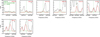	Fig. 3 Same as Fig. 2 but for source G345.5043+00.3480 with broad lines (FWHM = 7.8 km s⁻¹).
In the text

Fig. 4

Summary of the detected species toward the sources. Plus signs show the detected and tentatively detected molecules and minus signs show the non-detections. The sources are ordered from left to right from the lowest to highest distance. The tentative detection of CH₃NH₂ in sources 707948 and 787212 is uncertain due to line blending and more data is needed for a more robust confirmation.

In the text

Fig. 5

Moment zero maps of four selected lines for four sources included in Fig. 1. The line, name of the source and E_up of the line are printed in white at the middle top of each panel. The beam is also shown on the bottom left of each panel. The continuum contours are shown in black and are at [3, 5, 10, 20, 30]σ_cont with σ_cont for the sources from top to bottom being 7.6, 4.1, 1.9 and 0.8 mJy beam⁻¹, respectively. The scale bars on the bottom right of each panel from top to bottom show lengths of 10942, 7199, 11518, and 39089 au at the distances of the sources.

In the text

	Fig. 6 Mean of the excitation temperatures of the species in sources where the temperature is fitted. The error bars are calculated as explained in the text. The species are ordered by their binding energies from low (left) to high (right). The dashed lines are to separate the three groups of species seen.
In the text

	Fig. 7 Correlation matrix for Pearson coefficient of the column densities. The darkest green shows the highest correlation. In this figure sources with their methanol column density found from ¹³CH₃OH are excluded due to optical depth effects.
In the text

Fig. 8

Column density of NH₂CHO versus column density of HNCO. Top panel: data points from the ALMAGAL survey found in this work with the best fit plotted as the middle solid line and the shaded green area showing the 68 percentile scatter in the data. Bottom panel: compares the fitted data in our work by studies from López-Sepulcre et al. (2015), Quénard et al. (2018), Ligterink et al. (2020), Law et al. (2021) and Colzi et al. (2021). The curves for López-Sepulcre et al. (2015), Quénard et al. (2018) and Colzi et al. (2021) are taken from the fit to abundances of NH₂CHO and HNCO and are normalized here as explained in the text: only slopes can be compared, not the absolute values.

In the text

Fig. 9

Column density ratio of C₂H₅CN to CH₃CN versus bolometric luminosity for low- and high-mass sources. The red points show the values for ALMAGAL sources from this work. Blue and pink show values for low- and high-mass protostars taken from the literature (see Table E.4 for the references). Moreover, the purple bar shows the range of C₂H₅CN/CH₃CN peak gas-phase values from Garrod et al. (2022) in the warm-up stages with slow, medium and fast pace (from their Table 17, final model setup). The purple arrow shows that the range of models are higher than the range in this plot. Upward triangles show lower limits and downward triangles show upper limits. Grey solid line and shaded gray area show the mean and standard deviation weighted by the uncertainty on the log₁₀ of each column density ratio after eliminating upper and lower limits. Moreover, Sgr B2(N2) is eliminated in the derivation of mean and standard deviation, as it often seems to be an outlier.

In the text

	Fig. 10 Same as Fig. 9, but for HNCO/CH₃CN. The literature values are taken from studies presented in Table E.4. In this plot SMM1-a is colored blue although it is an intermediate mass protostar.
In the text

	Fig. 11 Same as Fig. 9, but for NH₂CHO/CH₃OH. The red hollow circles indicate the sources for which ¹³CH₃OH was used to find the column density of CH₃OH.
In the text

Fig. 12

One σ scatter around the mean of log₁₀ of the column density ratios. Both mean and standard deviation are weighted by the errors on each data point. Blue shows the values for low-mass protostars where there were more than two sources available for this calculation. Red shows the scatter for high-mass protostars and black presents those for all sources available (i.e., low- and high-mass protostars).

In the text

	Fig. 13 Cartoon of two sources: one with disk (left) and one without (right). The red and blue regions show the emitting regions of NH₂CHO and CH₃OH, respectively. There is not a priory reason as to why the ratio of the two sublimation regions between the two sources should remain constant.
In the text

	Fig. 14 Factor of spread around the mean of the pre-stellar timescales for various low- and high-mass protostars using the spread factor found for low-mass, ALMAGAL and high-mass literature sources (see black points in Fig. 12).
In the text

	Fig. D.1 Demonstration of how excitation temperature upper and lower bounds are determined for NH₂CHO for source 767784. The various symbols are the same as Fig. 2.
In the text

	Fig. D.2 Demonstration of how excitation temperature upper and lower bounds are determined for ${CH}_{3}^{18} OH$ ${\rm{CH}}_{\rm{3}}^{{\rm{18}}}{\rm{OH}}$ for source 767784. The various symbols are the same as Fig. 2.
In the text

	Fig. D.3 Showing that excitation temperature of 60 K does not match the observations for CH₃NH₂ in source 767784. The various symbols are the same as Fig. 2. Here a few lines are overestimated, for example, the ones with E_up of 17.3 K and 92.2 K and if the column density is decreased lines such as the ones with E_up of 156.5 K and 182.1 K will be underestimated.
In the text

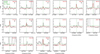	Fig. D.4 Best-fit model for CH₃NH₂ in source 767784. The various symbols are the same as Fig. 2.
In the text

	Fig. D.5 Showing that excitation temperature of 150 K does not match the observations for CH₃NH₂ in source 767784. The various symbols are the same as Fig. 2. Again here some lines are overestimated and if the column density is decreased the lines that are perfect fits now will be underestimated.
In the text

Fig. D.6

Best model for HN¹³CO of source 881427 (red) on top of the data (black). In this figure only lines with A_ij > 10⁻⁶ s⁻¹ and E_up < 700 K are shown. Moreover, only one representative plot of the hyper fine structure of this molecule is shown to avoid repetition. The detected lines that are mainly considered for the fits are marked with an ‘X’ on the top right. The dashed lines shows the 3σ line.

In the text

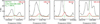	Fig. D.7 Same as Fig. D.6, but for G345.5043+00.3480.
In the text

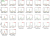	Fig. D.8 Same as Fig. D.6, but for C₂H₅CN.
In the text

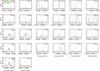	Fig. D.9 Same as Fig. D.6, but for G345.5043+00.3480 and C₂H₅CN.
In the text

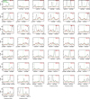	Fig. D.10 Same as Fig. D.6, but for C₂H₃CN.
In the text

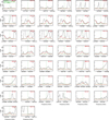	Fig. D.11 Same as Fig. D.6, but for G345.5043+00.3480 and C₂H₃CN.
In the text

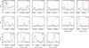	Fig. D.12 Same as Fig. D.6, but for CH₃NH₂.
In the text

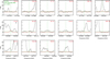	Fig. D.13 Same as Fig. D.6, but for G345.5043+00.3480 and CH₃NH₂.
In the text

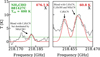	Fig. D.14 Same as Fig. D.6, but for NH₂CHO. Here only lines with A_ij > 10⁻⁵ s⁻¹ are shown.
In the text

	Fig. D.15 Same as Fig. D.6, but for G345.5043+00.3480 and NH₂CHO. Here only lines with A_ij > 10⁻⁵ s⁻¹ are shown.
In the text

	Fig. D.16 Same as Fig. 4, but now the sources are ordered from left to right from the lowest to highest luminosity.
In the text

	Fig. D.17 Correlations seen in column densities. Column densities of the molecules considered in this work plotted versus each other. Only detected molecules are plotted here. The Pearson’s r coefficient is given at the top left of each panel.
In the text

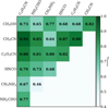	Fig. D.18 Same as Fig. 7, but column densities of methanol found from ¹³CH₃OH are also included.
In the text

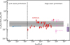	Fig. D.19 Same as Fig. 9, but for C₂H₃CN/C₂H₅CN. The references are given in Table E.4.
In the text

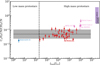	Fig. D.20 Same as Fig. 9, but for C₂H₃CN/CH₃CN. The references are given in Table E.4.
In the text

	Fig. D.21 Same as Fig. 9, but for HNCO/CH₃OH. In this plot SMM1-a is colored blue although it is an intermediate mass protostar. The references are given in Table E.4. The red hollow circles indicate the sources for which ¹³CH₃OH was used to find the column density of CH₃OH.
In the text

	Fig. D.22 Same as Fig. 9, but for CH₃CN/CH₃OH. In this plot SMM1-a is colored blue although it is an intermediate mass protostar. The references are given in Table E.4. The red hollow circles indicate the sources for which ¹³CH₃OH was used to find the column density of CH₃OH.
In the text

	Fig. D.23 Same as Fig. 9, but for CH₃NH₂/CH₃OH. The references are given in Table E.4. The red hollow circles indicate the sources for which ¹³CH₃OH was used to find the column density of CH₃OH.
In the text

	Fig. D.24 Same as Fig. 9, but for CH₃NH₂/HNCO. The references are given in Table E.4. The luminosity for source G+0.693 is assumed at 10⁴ as no estimation of the luminosity was found for this source.
In the text

	Fig. D.25 Same as Fig. 9, but for CH₃NH₂/CH₃CN. The references are given in Table E.4. The luminosity for source G+0.693 is assumed at 10⁴ as no estimation of the luminosity was found for this source.
In the text

	Fig. D.26 Same as Fig. 9, but for CH₃NH₂/NH₂CHO. The references are given in Table E.4. The luminosity for source G+0.693 is assumed at 10⁴ as no estimation of the luminosity was found for this source.
In the text

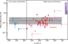	Fig. D.27 Same as Fig. 9, but for NH₂CHO/CH₃CN. The references are given in Table E.4.
In the text

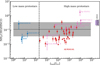	Fig. D.28 Same as Fig. 9, but for NH₂CHO/HNCO. The references are given in Table E.4.
In the text

	Fig. D.29 Spread highlighted in Fig. 9 (gray) is over plotted with values from Table 15 of Garrod et al. (2022) that show the peak gas phase abundances of a few N-bearing species during their warm up phase (blue).
In the text

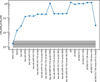	Fig. D.30 Same as Fig. D.29, but for CH₃NH₂/CH₃OH.
In the text

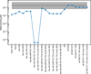	Fig. D.31 Same as Fig. D.29, but for HNCO/CH₃OH.
In the text

	Fig. D.32 Abundances assumed for the toy model.
In the text

Current usage metrics show cumulative count of Article Views (full-text article views including HTML views, PDF and ePub downloads, according to the available data) and Abstracts Views on Vision4Press platform.

Data correspond to usage on the plateform after 2015. The current usage metrics is available 48-96 hours after online publication and is updated daily on week days.

Initial download of the metrics may take a while.

[1] Aikawa, Y., Furuya, K., Yamamoto, S., & Sakai, N. 2020, ApJ, 897, 110 [Google Scholar]

[2] Anttila, R., Horneman, V. M., Koivusaari, M., & Paso, R. 1993, J. Mol. Spectr., 157, 198 [Google Scholar]

[3] Barone, V., Latouche, C., Skouteris, D., et al. 2015, MNRAS, 453, L31 [Google Scholar]

[4] Baskakov, O. I., Dyubko, S. F., Ilyushin, V. V., et al. 1996, J. Mol. Spectr., 179, 94 [NASA ADS] [CrossRef] [Google Scholar]

[5] Belloche, A., Müller, H. S. P., Menten, K. M., Schilke, P., & Comito, C. 2013, A&A, 559, A47 [NASA ADS] [CrossRef] [EDP Sciences] [Google Scholar]

[6] Belloche, A., Müller, H. S. P., Garrod, R. T., & Menten, K. M. 2016, A&A, 587, A91 [NASA ADS] [CrossRef] [EDP Sciences] [Google Scholar]

[7] Belloche, A., Meshcheryakov, A. A., Garrod, R. T., et al. 2017, A&A, 601, A49 [NASA ADS] [CrossRef] [EDP Sciences] [Google Scholar]

[8] Belloche, A., Maury, A. J., Maret, S., et al. 2020, A&A, 635, A198 [NASA ADS] [CrossRef] [EDP Sciences] [Google Scholar]

[9] Beltrán, M. T., Codella, C., Viti, S., Neri, R., & Cesaroni, R. 2009, ApJ, 690, L93 [Google Scholar]

[10] Bertin, M., Doronin, M., Fillion, J. H., et al. 2017, A&A, 598, A18 [NASA ADS] [CrossRef] [EDP Sciences] [Google Scholar]

[11] Bianchi, E., López-Sepulcre, A., Ceccarelli, C., et al. 2022, ApJ, 928, L3 [NASA ADS] [CrossRef] [Google Scholar]

[12] Bisschop, S. E., Jørgensen, J. K., van Dishoeck, E. F., & de Wachter, E. B. M. 2007, A&A, 465, 913 [NASA ADS] [CrossRef] [EDP Sciences] [Google Scholar]

[13] Bisschop, S. E., Jørgensen, J. K., Bourke, T. L., Bottinelli, S., & van Dishoeck, E. F. 2008, A&A, 488, 959 [NASA ADS] [CrossRef] [EDP Sciences] [Google Scholar]

[14] Blake, G. A., Sutton, E. C., Masson, C. R., & Phillips, T. G. 1987, ApJ, 315, 621 [Google Scholar]

[15] Bøgelund, E. G., McGuire, B. A., Ligterink, N. F. W., et al. 2018, A&A, 615, A88 [Google Scholar]

[16] Bøgelund, E. G., Barr, A. G., Taquet, V., et al. 2019a, A&A, 628, A2 [NASA ADS] [CrossRef] [EDP Sciences] [Google Scholar]

[17] Bøgelund, E. G., McGuire, B. A., Hogerheijde, M. R., van Dishoeck, E. F., & Ligterink, N. F. W. 2019b, A&A, 624, A82 [EDP Sciences] [Google Scholar]

[18] Boogert, A. C. A., Pontoppidan, K. M., Knez, C., et al. 2008, ApJ, 678, 985 [Google Scholar]

[19] Boogert, A. C. A., Gerakines, P. A., & Whittet, D. C. B. 2015, ARA&A, 53, 541 [Google Scholar]

[20] Bottinelli, S., Ceccarelli, C., Lefloch, B., et al. 2004, ApJ, 615, 354 [Google Scholar]

[21] Boucher, D., Burie, J., Demaison, J., et al. 1977, J. Mol. Spectr., 64, 290 [NASA ADS] [CrossRef] [Google Scholar]

[22] Boucher, D., Dubrulle, A., Demaison, J., & Dreizler, H. 1980, Z. Nat. Teil A, 35, 1136 [NASA ADS] [Google Scholar]

[23] Bulak, M., Paardekooper, D. M., Fedoseev, G., & Linnartz, H. 2021, A&A, 647, A82 [NASA ADS] [CrossRef] [EDP Sciences] [Google Scholar]

[24] Calcutt, H., Jørgensen, J. K., Müller, H. S. P., et al. 2018, A&A, 616, A90 [NASA ADS] [CrossRef] [EDP Sciences] [Google Scholar]

[25] Cazaux, S., Tielens, A. G. G. M., Ceccarelli, C., et al. 2003, ApJ, 593, L51 [NASA ADS] [CrossRef] [Google Scholar]

[26] Cazzoli, G., & Kisiel, Z. 1988, J. Mol. Spectr., 130, 303 [NASA ADS] [CrossRef] [Google Scholar]

[27] Cazzoli, G., & Puzzarini, C. 2006, J. Mol. Spectr., 240, 153 [NASA ADS] [CrossRef] [Google Scholar]

[28] Cernicharo, J., Kisiel, Z., Tercero, B., et al. 2016, A&A, 587, L4 [NASA ADS] [CrossRef] [EDP Sciences] [Google Scholar]

[29] Chaabouni, H., Diana, S., Nguyen, T., & Dulieu, F. 2018, A&A, 612, A47 [NASA ADS] [CrossRef] [EDP Sciences] [Google Scholar]

[30] Chuang, K. J., Fedoseev, G., Scirè, C., et al. 2021, A&A, 650, A85 [NASA ADS] [CrossRef] [EDP Sciences] [Google Scholar]

[31] Codella, C., Ceccarelli, C., Caselli, P., et al. 2017, A&A, 605, L3 [NASA ADS] [CrossRef] [EDP Sciences] [Google Scholar]

[32] Coletta, A., Fontani, F., Rivilla, V. M., et al. 2020, A&A, 641, A54 [NASA ADS] [CrossRef] [EDP Sciences] [Google Scholar]

[33] Collings, M. P., Anderson, M. A., Chen, R., et al. 2004, MNRAS, 354, 1133 [NASA ADS] [CrossRef] [Google Scholar]

[34] Colmont, J. M., Wlodarczak, G., Priem, D., et al. 1997, J. Mol. Spectr., 181, 330 [NASA ADS] [CrossRef] [Google Scholar]

[35] Colzi, L., Rivilla, V. M., Beltrán, M. T., et al. 2021, A&A, 653, A129 [NASA ADS] [CrossRef] [EDP Sciences] [Google Scholar]

[36] Coutens, A., Jørgensen, J. K., van der Wiel, M. H. D., et al. 2016, A&A, 590, L6 [NASA ADS] [CrossRef] [EDP Sciences] [Google Scholar]

[37] Das, A., Sil, M., Gorai, P., Chakrabarti, S. K., & Loison, J. C. 2018, ApJS, 237, 9 [NASA ADS] [CrossRef] [Google Scholar]

[38] Davies, B., Hoare, M. G., Lumsden, S. L., et al. 2011, MNRAS, 416, 972 [Google Scholar]

[39] Demaison, J., Dubrulle, A., Boucher, D., Burie, J., & Typke, V. 1979, J. Mol. Spectr., 76, 1 [NASA ADS] [CrossRef] [Google Scholar]

[40] Demaison, J., Cosleou, J., Bocquet, R., & Lesarri, A. G. 1994, J. Mol. Spectr., 167, 400 [NASA ADS] [CrossRef] [Google Scholar]

[41] Dulieu, F., Nguyen, T., Congiu, E., Baouche, S., & Taquet, V. 2019, MNRAS, 484, L119 [NASA ADS] [CrossRef] [Google Scholar]

[42] Elia, D., Molinari, S., Schisano, E., et al. 2017, MNRAS, 471, 100 [NASA ADS] [CrossRef] [Google Scholar]

[43] Elia, D., Merello, M., Molinari, S., et al. 2021, MNRAS, 504, 2742 [NASA ADS] [CrossRef] [Google Scholar]

[44] Fedoseev, G., Chuang, K. J., van Dishoeck, E. F., Ioppolo, S., & Linnartz, H. 2016, MNRAS, 460, 4297 [Google Scholar]

[45] Fedoseev, G., Chuang, K. J., Ioppolo, S., et al. 2017, ApJ, 842, 52 [Google Scholar]

[46] Ferrero, S., Zamirri, L., Ceccarelli, C., et al. 2020, ApJ, 904, 11 [NASA ADS] [CrossRef] [Google Scholar]

[47] Fontani, F., Pascucci, I., Caselli, P., et al. 2007, A&A, 470, 639 [NASA ADS] [CrossRef] [EDP Sciences] [Google Scholar]

[48] Förstel, M., Bergantini, A., Maksyutenko, P., Góbi, S., & Kaiser, R. I. 2017, ApJ, 845, 83 [Google Scholar]

[49] Fuchs, G. W., Cuppen, H. M., Ioppolo, S., et al. 2009, A&A, 505, 629 [NASA ADS] [CrossRef] [EDP Sciences] [Google Scholar]

[50] Fukuyama, Y., Odashima, H., Takagi, K., & Tsunekawa, S. 1996, ApJS, 104, 329 [NASA ADS] [CrossRef] [Google Scholar]

[51] Garrod, R. T. 2013, ApJ, 765, 60 [Google Scholar]

[52] Garrod, R. T., Widicus Weaver, S. L., & Herbst, E. 2008, ApJ, 682, 283 [Google Scholar]

[53] Garrod, R. T., Belloche, A., Müller, H. S. P., & Menten, K. M. 2017, A&A, 601, A48 [NASA ADS] [CrossRef] [EDP Sciences] [Google Scholar]

[54] Garrod, R. T., Jin, M., Matis, K. A., et al. 2022, ApJS, 259, 1 [NASA ADS] [CrossRef] [Google Scholar]

[55] Gerry, M. C. L., & Winnewisser, G. 1973, J. Mol. Spectr., 48, 1 [NASA ADS] [CrossRef] [Google Scholar]

[56] Gibb, E., Nummelin, A., Irvine, W. M., Whittet, D. C. B., & Bergman, P. 2000, ApJ, 545, 309 [NASA ADS] [CrossRef] [Google Scholar]

[57] Gorai, P., Bhat, B., Sil, M., et al. 2020, ApJ, 895, 86 [Google Scholar]

[58] Gorai, P., Das, A., Shimonishi, T., et al. 2021, ApJ, 907, 108 [NASA ADS] [CrossRef] [Google Scholar]

[59] Grim, R. J. A., & Greenberg, J. M. 1987, ApJ, 321, L91 [NASA ADS] [CrossRef] [Google Scholar]

[60] Grim, R. J. A., Baas, F., Geballe, T. R., Greenberg, J. M., & Schutte, W. A. 1991, A&A, 243, 473 [NASA ADS] [Google Scholar]

[61] Haupa, K. A., Tarczay, G., & Lee, Y.-P. 2019, J. Am. Chem. Soc., 141, 11614 [CrossRef] [Google Scholar]

[62] Heise, H. M., Winther, F., & Lutz, H. 1981, J. Mol. Spectr., 90, 531 [NASA ADS] [CrossRef] [Google Scholar]

[63] Herbst, E., & van Dishoeck, E. F. 2009, ARA&A, 47, 427 [NASA ADS] [CrossRef] [Google Scholar]

[64] Hirota, E., Sugisaki, R., Nielsen, C. J., & Sørensen, G. O. 1974, J. Mol. Spectr., 49, 251 [NASA ADS] [CrossRef] [Google Scholar]

[65] Hocking, W. H., Gerry, M. C. L., & Winnewisser, G. 1975, Canadian J. Phys., 53, 1869 [NASA ADS] [CrossRef] [Google Scholar]

[66] Honma, M., Nagayama, T., & Sakai, N. 2015, PASJ, 67, 70 [NASA ADS] [CrossRef] [Google Scholar]

[67] Hsu, S.-Y., Liu, S.-Y., Liu, T., et al. 2022, ApJ, 927, 218 [NASA ADS] [CrossRef] [Google Scholar]

[68] Hudson, R. L., & Moore, M. H. 2004, Icarus, 172, 466 [Google Scholar]

[69] Ilyushin, V. V., Alekseev, E. A., Dyubko, S. F., Motiyenko, R. A., & Hougen, J. T. 2005, J. Mol. Spectr., 229, 170 [NASA ADS] [CrossRef] [Google Scholar]

[70] Jaber, A. A., Ceccarelli, C., Kahane, C., & Caux, E. 2014, ApJ, 791, 29 [Google Scholar]

[71] Jacobsen, S. K., Jørgensen, J. K., Di Francesco, J., et al. 2019, A&A, 629, A29 [NASA ADS] [CrossRef] [EDP Sciences] [Google Scholar]

[72] Johnson, D. R., Lovas, F. J., Gottlieb, C. A., et al. 1977, ApJ, 218, 370 [NASA ADS] [CrossRef] [Google Scholar]

[73] Jones, B. M., Bennett, C. J., & Kaiser, R. I. 2011, ApJ, 734, 78 [Google Scholar]

[74] Jørgensen, J. K., Schöier, F. L., & van Dishoeck, E. F. 2005, A&A, 435, 177 [NASA ADS] [CrossRef] [EDP Sciences] [Google Scholar]

[75] Jørgensen, J. K., van der Wiel, M. H. D., Coutens, A., et al. 2016, A&A, 595, A117 [Google Scholar]

[76] Jørgensen, J. K., Müller, H. S. P., Calcutt, H., et al. 2018, A&A, 620, A170 [Google Scholar]

[77] Kahane, C., Ceccarelli, C., Faure, A., & Caux, E. 2013, ApJ, 763, L38 [CrossRef] [Google Scholar]

[78] Kaifu, N., Morimoto, M., Nagane, K., et al. 1974, ApJ, 191, L135 [Google Scholar]

[79] Kim, Y. S., & Kaiser, R. I. 2011, ApJ, 729, 68 [NASA ADS] [CrossRef] [Google Scholar]

[80] Kréglewski, M., & Wlodarczak, G. 1992, J. Mol. Spectr., 156, 383 [CrossRef] [Google Scholar]

[81] Kręglewski, M., Stahl, W., Grabow, J.-U., & Wlodarczak, G. 1992, Chem. Phys. Lett., 196, 155 [CrossRef] [Google Scholar]

[82] Kryvda, A. V., Gerasimov, V. G., Dyubko, S. F., Alekseev, E. A., & Motiyenko, R. A. 2009, J. Mol. Spectr., 254, 28 [NASA ADS] [CrossRef] [Google Scholar]

[83] Kukolich, S. G. 1982, J. Chem. Phys., 76, 97 [NASA ADS] [CrossRef] [Google Scholar]

[84] Kukolich, S. G., & Nelson, A. C. 1971, Chem. Phys. Lett., 11, 383 [NASA ADS] [CrossRef] [Google Scholar]

[85] Kukolich, S. G., Ruben, D. J., Wang, J. H. S., & Williams, J. R. 1973, J. Chem. Phys., 58, 3155 [NASA ADS] [CrossRef] [Google Scholar]

[86] Law, C. J., Zhang, Q., Öberg, K. I., et al. 2021, ApJ, 909, 214 [Google Scholar]

[87] Lee, J.-E., Evans, Neal J.I., Shirley, Y. L., & Tatematsu, K. 2003, ApJ, 583, 789 [NASA ADS] [CrossRef] [Google Scholar]

[88] Lee, C.-F., Codella, C., Li, Z.-Y., & Liu, S.-Y. 2019, ApJ, 876, 63 [Google Scholar]

[89] Lees, R. M., & Baker, J. G. 1968, J. Chem. Phys., 48, 5299 [NASA ADS] [CrossRef] [Google Scholar]

[90] Ligterink, N. F. W., Coutens, A., Kofman, V., et al. 2017, MNRAS, 469, 2219 [Google Scholar]

[91] Ligterink, N. F. W., Calcutt, H., Coutens, A., et al. 2018, A&A, 619, A28 [NASA ADS] [CrossRef] [EDP Sciences] [Google Scholar]

[92] Ligterink, N. F. W., El-Abd, S. J., Brogan, C. L., et al. 2020, ApJ, 901, 37 [Google Scholar]

[93] Ligterink, N. F. W., Ahmadi, A., Coutens, A., et al. 2021, A&A, 647, A87 [NASA ADS] [CrossRef] [EDP Sciences] [Google Scholar]

[94] López-Sepulcre, A., Jaber, A. A., Mendoza, E., et al. 2015, MNRAS, 449, 2438 [CrossRef] [Google Scholar]

[95] López-Sepulcre, A., Sakai, N., Neri, R., et al. 2017, A&A, 606, A121 [NASA ADS] [CrossRef] [EDP Sciences] [Google Scholar]

[96] López-Sepulcre, A., Balucani, N., Ceccarelli, C., et al. 2019, ACS Earth Space Chem., 3, 2122 [CrossRef] [Google Scholar]

[97] Lumsden, S. L., Hoare, M. G., Urquhart, J. S., et al. 2013, ApJS, 208, 11 [Google Scholar]

[98] Mäder, H., Heise, H. M., & Dreizler, H. 1974, Z. Nat. Teil A, 29, 164 [Google Scholar]

[99] Manigand, S., Jørgensen, J. K., Calcutt, H., et al. 2020, A&A, 635, A48 [NASA ADS] [CrossRef] [EDP Sciences] [Google Scholar]

[100] Martín-Doménech, R., Öberg, K. I., & Rajappan, M. 2020, ApJ, 894, 98 [Google Scholar]

[101] McGuire, B. A. 2022, ApJ Supplement Series, 259, 30 [NASA ADS] [CrossRef] [Google Scholar]

[102] McMullin, J. P., Waters, B., Schiebel, D., Young, W., & Golap, K. 2007, ASP Conf. Ser., 376, 127 [Google Scholar]

[103] Mège, P., Russeil, D., Zavagno, A., et al. 2021, A&A, 646, A74 [NASA ADS] [CrossRef] [EDP Sciences] [Google Scholar]

[104] Milam, S. N., Savage, C., Brewster, M. A., Ziurys, L. M., & Wyckoff, S. 2005, ApJ, 634, 1126 [Google Scholar]

[105] Minissale, M., Aikawa, Y., Bergin, E., et al. 2022, ACS Earth Space Chem., 6, 597 [NASA ADS] [CrossRef] [Google Scholar]

[106] Molet, J., Brouillet, N., Nony, T., et al. 2019, A&A, 626, A132 [EDP Sciences] [Google Scholar]

[107] Molinari, S., Swinyard, B., Bally, J., et al. 2010, A&A, 518, L100 [NASA ADS] [CrossRef] [EDP Sciences] [Google Scholar]

[108] Moskienko, E. M., & Dyubko, S. F. 1991, Radiophys. Quant. Electron., 34, 181 [NASA ADS] [CrossRef] [Google Scholar]

[109] Motiyenko, R. A., Tercero, B., Cernicharo, J., & Margulès, L. 2012, A&A, 548, A71 [NASA ADS] [CrossRef] [EDP Sciences] [Google Scholar]

[110] Motte, F., Bontemps, S., & Louvet, F. 2018, ARA&A, 56, 41 [NASA ADS] [CrossRef] [Google Scholar]

[111] Mottram, J. C., Hoare, M. G., Davies, B., et al. 2011, ApJ, 730, L33 [Google Scholar]

[112] Müller, H. S. P., Thorwirth, S., Roth, D. A., & Winnewisser, G. 2001, A&A, 370, L49 [Google Scholar]

[113] Müller, H. S. P., Schlöder, F., Stutzki, J., & Winnewisser, G. 2005, J. Mol. Struc., 742, 215 [Google Scholar]

[114] Müller, H. S. P., Belloche, A., Menten, K. M., Comito, C., & Schilke, P. 2008, J. Mol. Spectr., 251, 319 [Google Scholar]

[115] Müller, H. S. P., Drouin, B. J., & Pearson, J. C. 2009, A&A, 506, 1487 [NASA ADS] [CrossRef] [EDP Sciences] [Google Scholar]

[116] Muller, S., Beelen, A., Guélin, M., et al. 2011, A&A, 535, A103 [NASA ADS] [CrossRef] [EDP Sciences] [Google Scholar]

[117] Müller, H. S. P., Brown, L. R., Drouin, B. J., et al. 2015, J. Mol. Spectr., 312, 22 [CrossRef] [Google Scholar]

[118] Nazari, P., van Gelder, M. L., van Dishoeck, E. F., et al. 2021, A&A, 650, A150 [EDP Sciences] [Google Scholar]

[119] Nazari, P., Tabone, B., Rosotti, G. P., et al. 2022, A&A, 663, A58 [NASA ADS] [CrossRef] [EDP Sciences] [Google Scholar]

[120] Neill, J. L., Bergin, E. A., Lis, D. C., et al. 2014, ApJ, 789, 8 [Google Scholar]

[121] Nishikawa, T. 1957, J. Phys. Soc. Japan, 12, 668 [NASA ADS] [CrossRef] [Google Scholar]

[122] Öberg, K. I., Garrod, R. T., van Dishoeck, E. F., & Linnartz, H. 2009, A&A, 504, 891 [NASA ADS] [CrossRef] [EDP Sciences] [Google Scholar]

[123] Öberg, K. I., Boogert, A. C. A., Pontoppidan, K. M., et al. 2011, ApJ, 740, 109 [Google Scholar]

[124] Ohashi, N., Takagi, K., Hougen, J. T., Olson, W. B., & Lafferty, W. J. 1987, J. Mol. Spectr., 126, 443 [Google Scholar]

[125] Ohishi, M., Suzuki, T., Hirota, T., Saito, M., & Kaifu, N. 2019, PASJ, 71, 86 [NASA ADS] [CrossRef] [Google Scholar]

[126] Pearson, J. C., & Mueller, H. S. P. 1996, ApJ, 471, 1067 [NASA ADS] [CrossRef] [Google Scholar]

[127] Pearson, J. C., Sastry, K. V. L. N., Herbst, E., & De Lucia, F. C. 1994, ApJS, 93, 589 [Google Scholar]

[128] Penteado, E. M., Walsh, C., & Cuppen, H. M. 2017, ApJ, 844, 71 [Google Scholar]

[129] Pickett, H. M., Cohen, E. A., Brinza, D. E., & Schaefer, M. M. 1981, J. Mol. Spectr., 89, 542 [NASA ADS] [CrossRef] [Google Scholar]

[130] Pickett, H. M., Poynter, R. L., Cohen, E. A., et al. 1998, J. Quant. Spectr Rad. Transf., 60, 883 [NASA ADS] [CrossRef] [Google Scholar]

[131] Pitts, R. L., Kristensen, L. E., Jørgensen, J. K., & van der Walt, S. J. 2022, A&A, 657, A70 [NASA ADS] [CrossRef] [EDP Sciences] [Google Scholar]

[132] Qasim, D., Fedoseev, G., Chuang, K. J., et al. 2019, A&A, 627, A1 [NASA ADS] [CrossRef] [EDP Sciences] [Google Scholar]

[133] Quénard, D., Jiménez-Serra, I., Viti, S., Holdship, J., & Coutens, A. 2018, MNRAS, 474, 2796 [Google Scholar]

[134] Raunier, S., Chiavassa, T., Duvernay, F., et al. 2004, A&A, 416, 165 [NASA ADS] [CrossRef] [EDP Sciences] [Google Scholar]

[135] Rimola, A., Skouteris, D., Balucani, N., et al. 2018, ACS Earth Space Chem., 2, 720 [Google Scholar]

[136] Rivilla, V. M., Beltrán, M. T., Cesaroni, R., et al. 2017, A&A, 598, A59 [NASA ADS] [CrossRef] [EDP Sciences] [Google Scholar]

[137] Sakai, N., & Yamamoto, S. 2013, Chem. Rev., 113, 8981 [Google Scholar]

[138] Schilke, P., Groesbeck, T. D., Blake, G. A., & Phillips, T. G. 1997, ApJS, 108, 301 [NASA ADS] [CrossRef] [Google Scholar]

[139] Schmalzl, M., Visser, R., Walsh, C., et al. 2014, A&A, 572, A81 [NASA ADS] [CrossRef] [EDP Sciences] [Google Scholar]

[140] Shimoda, K., Nishikawa, T., & Itoh, T. 1954, J. Phys. Soc. Japan, 9, 974 [NASA ADS] [CrossRef] [Google Scholar]

[141] Skouteris, D., Vazart, F., Ceccarelli, C., et al. 2017, MNRAS, 468, L1 [NASA ADS] [Google Scholar]

[142] Snow, T. P., & McCall, B. J. 2006, ARA&A, 44, 367 [NASA ADS] [CrossRef] [Google Scholar]

[143] Song, L., & Kästner, J. 2016, Phys. Chem. Chem. Phys., 18, 29278 [NASA ADS] [CrossRef] [Google Scholar]

[144] Stolze, M., & Sutter, D. H. 1985, Z. Natur. Teil A, 40, 998 [NASA ADS] [CrossRef] [Google Scholar]

[145] Taban, I. M., Schutte, W. A., Pontoppidan, K. M., & van Dishoeck, E. F. 2003, A&A, 399, 169 [NASA ADS] [CrossRef] [EDP Sciences] [Google Scholar]

[146] Takagi, K., & Kojima, T. 1971, J. Phys. Soc. Japan, 30, 1145 [NASA ADS] [CrossRef] [Google Scholar]

[147] Taniguchi, K., Guzmán, A. E., Majumdar, L., Saito, M., & Tokuda, K. 2020, ApJ, 898, 54 [Google Scholar]

[148] Theulé, P., Duvernay, F., Danger, G., et al. 2013, Adv. Space Res., 52, 1567 [CrossRef] [Google Scholar]

[149] Turner, B. E. 1991, ApJS, 76, 617 [NASA ADS] [CrossRef] [Google Scholar]

[150] Tychoniec, Ł., van Dishoeck, E. F., van’t Hoff, M. L. R., et al. 2021, A&A, 655, A65 [NASA ADS] [CrossRef] [EDP Sciences] [Google Scholar]

[151] van Broekhuizen, F. A., Keane, J. V., & Schutte, W. A. 2004, A&A, 415, 425 [NASA ADS] [CrossRef] [EDP Sciences] [Google Scholar]

[152] van Broekhuizen, F. A., Pontoppidan, K. M., Fraser, H. J., & van Dishoeck, E. F. 2005, A&A, 441, 249 [NASA ADS] [CrossRef] [EDP Sciences] [Google Scholar]

[153] van Dishoeck, E. F., Blake, G. A., Jansen, D. J., & Groesbeck, T. D. 1995, ApJ, 447, 760 [Google Scholar]

[154] van Gelder, M. L., Tabone, B., Tychoniec, Ł., et al. 2020, A&A, 639, A87 [NASA ADS] [CrossRef] [EDP Sciences] [Google Scholar]

[155] van Gelder, M. L., Jaspers, J., Nazari, P., et al. 2022a, A&A, 667, A136 [NASA ADS] [CrossRef] [EDP Sciences] [Google Scholar]

[156] van Gelder, M. L., Nazari, P., Tabone, B., et al. 2022b, A&A, 662, A67 [NASA ADS] [CrossRef] [EDP Sciences] [Google Scholar]

[157] van’t Hoff, M. L. R., Harsono, D., Tobin, J. J., et al. 2020, ApJ, 901, 166 [Google Scholar]

[158] Vastel, C., Bottinelli, S., Caux, E., Glorian, J. M., & Boiziot, M. 2015, in SF2A-2015: Proceedings of the Annual meeting of the French Society of Astronomy and Astrophysics, 313 [Google Scholar]

[159] Vorob’eva, E. M., & Dyubko, S. F. 1994, Radiophys. Quant. Electron., 37, 155 [Google Scholar]

[160] Wakelam, V., Loison, J. C., Mereau, R., & Ruaud, M. 2017, Mol. Astrophys., 6, 22 [NASA ADS] [CrossRef] [Google Scholar]

[161] Williams, G. M., Cyganowski, C. J., Brogan, C. L., et al. 2022, MNRAS, 509, 748 [Google Scholar]

[162] Wilson, T. L., & Rood, R. 1994, ARA&A, 32, 191 [Google Scholar]

[163] Xu, L.-H., Fisher, J., Lees, R. M., et al. 2008, J. Mol. Spectr., 251, 305 [NASA ADS] [CrossRef] [Google Scholar]