| Issue |
A&A
Volume 650, June 2021
|
|
|---|---|---|
| Article Number | A76 | |
| Number of page(s) | 29 | |
| Section | Extragalactic astronomy | |
| DOI | https://doi.org/10.1051/0004-6361/202038738 | |
| Published online | 09 June 2021 | |
H I content in Coma cluster substructure⋆
1
Kapteyn Astronomical Institute, University of Groningen, Landleven 12, 9747 AV Groningen, The Netherlands
e-mail: This email address is being protected from spambots. You need JavaScript enabled to view it.
2
Department of Astronomy, University of Cape Town, Private Bag X3, Rondebosch, 7701, South Africa
3
Netherlands Institute for Radio Astronomy (ASTRON), Oude Hoogeveensedijk 4, 7991 PD Dwingeloo, The Netherlands
4
INAF – Osservatorio Astronomico di Cagliari, Via della Scienza 5, 09047 Selargius, CA, Italy
5
Korea Astronomy and Space Science, Institute, 776 Daedeok-daero, Yuseong-gu, Daejeon 34055, Korea
6
South African Radio Astronomy Observatory, 2 Fir Street, Black River Park, Observatory, Cape Town 7925, South Africa
7
Department of Physics and Electronics, Rhodes University, PO Box 94 Makhanda 6140, South Africa
8
Argelander-Institut für Astronomie, Auf dem Hügel 71, 53121 Bonn, Germany
Received:
24
June
2020
Accepted:
3
November
2020
Abstract
Context. Galaxy clusters are some of largest structures in the universe. These very dense environments tend to be home to higher numbers of evolved galaxies than found in lower-density environments. It is well known that dense environments can influence the evolution of galaxies through the removal of the neutral gas (H I) reservoirs that fuel star formation. It is unclear which environment has a stronger effect: the local environment (i.e., the substructure within the cluster), or the cluster itself.
Aims. Using the new H I data from the Westerbork Coma Survey, we explore the average H I content of galaxies across the cluster comparing galaxies that reside in substructure to those that do not.
Methods. We applied the Dressler–Shectman test to our newly compiled redshift catalogue of the Coma cluster to search for substructure. With so few of the Coma galaxies directly detected in H I, we used the H I stacking technique to probe the average H I content below what can be directly detected.
Results. Using the Dressler–Shectman test, we find 15 substructures within the footprint of the Westerbork Coma Survey. We compare the average H I content for galaxies within substructure to those not in substructure. Using the H I stacking technique, we find that those Coma galaxies not detected in H I are more than 10–50 times more H I deficient than expected, which supports the scenario of an extremely efficient and rapid quenching mechanism. By studying the galaxies that are not directly detected in H I, we also find Coma to be more H I deficient than previously thought.
Key words: galaxies: clusters: general / galaxies: evolution / galaxies: groups: general / galaxies: general
Full Table C.1 is only available at the CDS via anonymous ftp to cdsarc.u-strasbg.fr (130.79.128.5) or via http://cdsarc.u-strasbg.fr/viz-bin/cat/J/A+A/650/A76
© ESO 2021
1. Introduction
In our current picture of cosmology, Λ cold dark matter (ΛCDM), larger structures (e.g., galaxy clusters) are built up through the hierarchical merging of smaller structures (e.g., galaxy groups or individual galaxies) (Springel et al. 2005). Using dark matter simulations, McGee et al. (2009) showed that 45% of galaxies accreted onto a Coma-sized cluster would have done so in groups. Their results suggest that the group environments play an important role in the evolution of galaxies prior to accretion onto the cluster. Traces of the accretion history of a cluster can be observed through substructure in the kinematics of the galaxies in the cluster (e.g., Dressler & Shectman 1988b; Hou et al. 2012). Observations have shown that roughly 30% of clusters contain kinematic substructure (Dressler & Shectman 1988b; Bird 1994; Hou et al. 2012). The observational evidence of substructure is further supported by dark matter simulations, which estimate that a similar fraction of clusters contain significant substructure (Knebe & Mueller 1999).
Given the prevalence of substructure within clusters, there have been many efforts to identify substructure. Groups of galaxies identified through substructure within the X-ray emission of the cluster (e.g., Neumann et al. 2001, 2003; Parekh et al. 2015; Zhang et al. 2009) may be older, more evolved groups that have had their own intra-cluster medium (ICM) prior to accretion onto the cluster. An alternative possibility is that the X-ray emission associated with such groups might not belong to them, but rather to the cluster ICM that was disturbed by the fast peri-centre passage of such recently accreted groups. Another identification method is a hierarchical clustering technique, a mathematical algorithm which sorts data into “clusters” based on an affinity parameter. This particular method, introduced by Serna & Gerbal (1996), assigns galaxies to groups by minimising the binding energy. However, one of the more common methods of identifying substructure is to look for kinematic deviations (δ values) between groups of galaxies and the cluster as a whole. This method is known as the Dressler–Shectman (DS) test (Dressler & Shectman 1988b). Aside from the original study in which Dressler & Shectman (1988b) looked for kinematic substructures in the Abell cluster catalogue, the DS test has been used to study the substructure in Abell 2192 and Abell 963 (Jaffé et al. 2013), the Antlia cluster (Hess et al. 2015), and the Coma cluster (Colless & Dunn 1996). All of the above methods are effective at finding substructure, however each method is sensitive to different density environments within a cluster. Knebe & Mueller (1999) studied the effectiveness of the DS test using numerical simulations of clusters and also compared the DS test to other methods such as the friends-of-friends (FoF) algorithm. These authors found that the DS test and FoF algorithm find similar structures, but there is a large scatter. Knebe & Mueller (1999) attributed the scatter (and also the differences in subgroups for the same cluster in the literature) to velocity projection effects that can artificially increase the δ values in the DS test.
Neumann et al. (2003) identified substructure in the Coma cluster by finding over-densities in the X-ray emission in the cluster. At the core of the cluster, these authors found an X-ray over-density associated with the two cD galaxies (NGC 4889 and NGC 4874). This X-ray over-density is offset from the X-ray centre of the cluster and has been attributed to the haloes of the individual galaxies (Andrade-Santos et al. 2013; Vikhlinin et al. 2001). Previous kinematic substructure analyses (e.g., Colless & Dunn 1996) have identified separate groups associated with NGC 4889 and NGC 4874. Colless & Dunn (1996) and White et al. (1993) suggested that the NGC 4889 group is merging with the NGC 4874 group, which was dislodged from the centre of the cluster potential as a result of the interaction. This would account for the velocity differences between the two galaxies themselves and also with respect to the cluster velocity.
Studies using the DS test and hierarchical clustering technique have found groups throughout the cluster, but both methods are sensitive to the availability of optical redshifts for a cluster (Adami et al. 2005). This is particularly evident when comparing the first DS test results from Dressler & Shectman (1988b), who found no significant substructure within the Coma cluster (their catalogue contained 100–200 galaxies over a 2 deg2 area), with later work on the Coma cluster by Colless & Dunn (1996), who found that there is significant substructure with a larger redshift catalogue over a similar area of the sky.
Identifying substructure within galaxy clusters is not only important to understand the build-up of the cluster, the local environments identified by substructure also provide insight into the evolution of galaxies (Neumann et al. 2001, 2003; Dressler & Shectman 1988b; Adami et al. 2005; Hess et al. 2015). Dressler (1980) found that galaxies residing in dense environments tend to be passive with more evolved morphologies, while low-density environments have higher fractions of less evolved, actively star-forming galaxies. This observed phenomenon is now referred to as the morphology–density relation. Uncovering the cause of the morphology–density relation is related to understanding the evolutionary pathway from late-type spiral (Sa/Sb/Sc/Sd) galaxies to early-type elliptical (dE/E) galaxies. On the traditional Hubble galaxy morphology ladder, lenticular (S0) galaxies bridge the gap between the ellipticals and the spirals. While S0s are thought to be quenched spirals (see Coccato et al. 2020, and references therein), it is not known how or even if S0s transition to elliptical galaxies. In cluster environments in which the fraction of S0 galaxies tends to be high, gas removal processes dominate the evolutionary mechanisms (see Aguerri 2012, for a review). It is still unclear which environment has a stronger effect in driving morphological evolution: Does the cluster drive these mechanisms, or are galaxies in groups pre-processed (e.g., Porter et al. 2008; Wilman et al. 2009; Zabludoff & Mulchaey 1998) prior to infall onto the cluster?
Studying the neutral gas (H I) in galaxies can provide an early picture of which environment (group or cluster) plays the strongest role in triggering the morphological evolution of galaxies as they migrate into clusters. The H I disc extends beyond the stellar disc of the galaxy (particularly in the field), making it the most susceptible to environmental interactions (e.g., Haynes & Giovanelli 1984; Serra et al. 2013; Jaffé et al. 2015). Strangulation, the process that removes gas from the halo thus halting the fresh supply of H I to the galaxy, is thought to be one of the main drivers behind the morphology–density relation (Balogh et al. 2000; Balogh & Morris 2000; Van Den Bosch et al. 2008). However, strangulation alone cannot fully explain the transition of galaxies from blue star-forming spiral galaxies to the red, passive lenticular and elliptical galaxies that dominate the galaxy clusters. The effects of galaxy harassment can completely destroy the discs of Sc/Sd galaxies such that the orbits of the constituent stars are affected. It is thought that this could explain the formation of dwarf elliptical (dE) galaxies that are prevalent in the centre of clusters (Mo et al. 2010). Ram-pressure stripping (Gunn et al. 1972; Chung et al. 2009; Kapferer et al. 2009; Abramson et al. 2011; Jaffé et al. 2015; Yoon et al. 2017) is the process by which the gas is stripped from the disc of a galaxy owing to its interaction with the intra-cluster or intra-group medium. Ram-pressure stripping is highly effective at rapidly removing the gas from the discs of galaxies, and could be a driving factor in affecting the transition of Sa/Sb to S0s (Mo et al. 2010). Signatures of these different processes affecting the evolution of galaxies are particularly evident in the H I. Strangulation results in a truncated or anaemic H I disc, while galaxies that have undergone ram-pressure stripping or harassment tend to have asymmetric H I discs or tails. The effectiveness of these processes in dense environments means that galaxies in clusters are more H I deficient than their field counterparts (e.g., Chung et al. 2009; Solanes et al. 1996).
The Coma cluster (Abell 1656), a nearby rich cluster, is one of the most well-studied galaxy clusters in the Universe (see Biviano et al. 1996, for historical review). One of the most comprehensive projects targeting Coma and spanning the entire electromagnetic spectrum, is the Coma Cluster Treasury Survey1 (CCTS). At the heart of the survey was an observing programme using the Advanced Camera for Surveys (ACS) on the Hubble Space Telescope (HST). The goal of the Coma ACS survey was to image the core and the infall region (Carter et al. 2008), however the observing programme was never completed owing to the failure of the ACS. While the HST imaging was never completed, contributions to the CCTS from observing programmes on other telescopes have provided rich insight into our understanding of the cluster and its population (e.g., Yagi et al. 2007, 2010; Smith et al. 2008).
At a distance of ∼100 Mpc and velocity dispersion of ∼1000 km s−1, Coma is the nearest large cluster to us. While Coma is often held up as a large, relaxed cluster, studies of its X-ray emission show a complex dynamical state (see Neumann et al. 2001, 2003, and references therein). There are many theories as to the formation of Coma, however the presence and difference in velocities of the two large cD galaxies (NGC 4874 and NGC 4889) at the centre of the cluster suggest that Coma is the result of a merger (Fitchett & Webster 1987). Coma has been the target of many redshift surveys in an effort to understand the distribution and kinematics of the galaxies within the cluster and identify any substructure (e.g., Colless & Dunn 1996; Chiboucas et al. 2010; Albareti et al. 2017). The presence of substructure in the cluster is now well established (e.g., Fitchett & Webster 1987; Mellier et al. 1988; Neumann et al. 2001, 2003; Adami et al. 2005). Many of the galaxy groups making up the substructure are thought to have been accreted onto the cluster, and in some cases could still be on first infall (e.g., Neumann et al. 2001, 2003; Adami et al. 2005).
There have also been a number of surveys of the H I content of galaxies in Coma, both targeted (e.g., Bravo-Alfaro et al. 2001; Gavazzi et al. 2006) and blind (e.g., Beijersbergen 2003; Haynes et al. 2018). These works have provided insight into the ongoing gas removal processes affecting the galaxies in the cluster, as well as an understanding of the H I deficiency of the cluster. The previous Coma H I surveys have lacked coverage, sensitivity, resolution, or some combination thereof. In this work, we use H I observations from the blind, high-sensitivity and high-resolution survey with the Westerbork Synthesis Radio Telescope (WSRT): the Westerbork Coma Survey (WCS; Molnar et al., in prep.). With the wealth of information already available, in combination with new H I observations of the cluster, we can explore the morphologies of the Coma galaxies in conjunction with their gas properties and local environment. Coma is known to be home to a large number of S0 galaxies: the relative fraction of S0s, ellipticals, spirals and mergers is 42%, 22%, 32%, and 4%, respectively (Beijersbergen 2003). This makes Coma an ideal laboratory to study H I properties of galaxies of different morphologies in the different local environments.
In this paper, we make use of data from a blind H I survey of the Coma cluster (Sect. 2.3) from Molnar et al. (in prep.) to study the H I gas properties of the different galaxy types in different environments within the cluster. Most of the galaxies in Coma are not individually detected in H I, thus we make use of the H I stacking technique (Sect. 3) to improve the signal-to-noise ratios (S/N) of groups of H I spectra. The optical spectroscopy and photometry used in this work are presented in Sect. 2. We explore the global H I properties of the galaxies in Coma by deriving optical–H I scaling relations and by determining the H I deficiency at different locations within the cluster (Sect. 4). We use the substructure within the cluster as a measure of the local environment (Sect. 5), and use H I stacking to probe the H I content of samples of galaxies within local environments relative to the global H I properties of the cluster (Sect. 6.4). Throughout this paper we use H0 = 70 km s−1 Mpc−1 (h = 0.7), Ωm = 0.7, and ΩΛ = 0.3.
2. Multiwavelength data
2.1. Optical spectroscopy
A full, wide-area redshift census of Coma is essential to this work for two reasons: First, H I stacking requires spectroscopic redshifts to align the H I non-detected spectra; second, we require redshifts in order to more accurately characterise the environment (substructure) within the cluster, as well any infalling groups. This work makes use of redshifts from two different sources: literature (Sect. 2.1.1) and spectroscopy obtained with Hydra at the WIYN Telescope2 (Sect. 2.1.2). The final catalogue contains 1095 spectroscopically confirmed members of the Coma cluster within a 2 deg radius of the cluster centre (58 are new redshifts – see Sect. 2.1.2); 850 of these fall within the WCS footprint (the orange outline in Fig. 2). The larger catalogue is necessary when looking for substructure within the cluster.
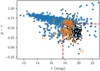 |
Fig. 1. Colour–magnitude diagram for the Coma cluster. The blue points represent the galaxies in the catalogue of literature redshifts. The black dots represent all galaxies targeted with Hydra, but whose redshifts place them in the foreground or background. The orange open squares represent the galaxies targeted with Hydra with redshifts that place them inside the cluster. Galaxies with r > 17.7 mag and g − r < 0.6 were prioritised as indicated by the dashed red lines. |
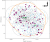 |
Fig. 2. WIYN/Hydra targets, and observed sources. The 5 fields (3 of the fields had a second configuration) targeted with WIYN are indicated by the large circles. The square and diamond data points represent the galaxies we targeted with Hydra. The galaxies with redshifts in the Coma volume are represented by the magenta square data points and the foreground and background galaxies are represented by the blue diamond markers. The green markers represent the three cD galaxies in Coma (+–NGC 4874, ⋎–NGC 4889 and ×–NGC 4839). The 0.4−2.4 keV ROSAT X-ray contours are given by the grey contours (outer contours correspond to 3 × 10⁻⁵ cts s−1, and inner-most contours to 1 × 10⁻³ cts s−1). Other confirmed members of the Coma cluster are represented by the small grey circles. The WCS footprint is indicated by the orange outline. |
2.1.1. Redshifts from the literature
The literature catalogue was collated from a number of published and unpublished catalogues. More than two-thirds of the redshifts were obtained from the Sloan Digital Sky Survey (SDSS) Data Release (DR) 13 (DR13; Albareti et al. 2017). The remainder come from a number of different sources (see Table A.1 for the number of redshifts from the different sources); the reference for each redshift is given in the Coma galaxy catalogue in Appendix C.
Using the VizieR astronomical catalogue database (Ochsenbein et al. 2000), we queried data in published catalogues within a 2 deg radius centred on the Coma cluster. Merging the SDSS redshifts with those obtained from VizierR created a large master catalogue with overlapping sources, some of which had redshifts outside of the Coma volume. To construct our catalogue of unique sources associated with the Coma cluster, we only consider sources with 3000 < cz < 10 500 km s−1 as this is the spectral range spanned by the H I data set. Sources within 5″ radius of each other are considered to be the same source; when multiple sources within the search radius were found, only the redshift with the smallest uncertainty was kept in the catalogue. Every galaxy with multiple redshift measurements was checked by eye so as not to remove the redshifts of real spatial overlapping galaxies.
2.1.2. Spectroscopy with Hydra
New spectroscopic data for galaxies in the Coma cluster was obtained using Hydra, the multi-object spectrograph, on the 3.5 m WIYN Telescope located at the Kitt Peak National Observatory. Despite being an extremely well-observed cluster, the spectroscopic coverage of Coma drops off for galaxies fainter than r ∼ 17.7 mag, thus we targeted galaxies fainter than this limit. Since previous targeted spectroscopic surveys have focussed on the core of the cluster, we prioritised galaxies with r > 17.7 mag on the outskirts of the cluster and with bluer colours (g − r < 0.6) as these are the galaxies we expect to contain H I. Figure 1 shows the colour magnitude diagram (CMD) for the cluster. The lower right quadrant of the CMD shows very few redshifts from literature, which is another motivation for targeting galaxies in that quadrant of the CMD. Initially, eight configurations of the five fields were targeted (three of the fields had a second configuration, which was necessary because of the density of targets); however owing to poor weather conditions on the first night, only six configurations were actually observed. The data were collected on the nights of 19–20 April 2018.
All the data reduction was done using IRAF3. The first phase of the data reduction after cosmic ray removal using lacosmic (van Dokkum 2001) was done using the ccdred package; this took care of the overscan, bias, and dark subtraction. The second phase was guided by the dohydra task, which takes care of the flat-fielding, aperture extraction, wavelength calibration, dispersion correction, and sky subtraction. The wavelength-calibrated and sky-subtracted spectra were then matched to template spectra to determine the redshift of the galaxies.
The redshift calculations were performed using the cross-correlation technique that is implemented by the IRAF task xcsao (Kurtz et al. 1992) contained within the rvsao package. We searched for velocities between 0 km s−1 and 100 000 km s−1 using seven different templates. We used three different types of emission line templates, three different types of absorption line templates, and one composite template so as to make sure we had covered the range in different types of stellar populations. Velocities were only accepted as robust if at least three templates produced results within 100 km s−1, a common uncertainty for a measurement based on absorption lines. The uncertainty on each redshift measurement was determined from the peak of the correlation between the template and observed spectrum. A detailed explanation can be found in Kurtz et al. (1992). All results were also inspected by eye. Three examples of Hydra spectra are shown in Fig. 3. The spectra have been sky-subtracted, but have not been flux calibrated as this is not necessary to obtain a redshift measurement; the vertical red bands indicate the regions of the spectra for which there are strong sky lines; and the dashed lines and grey regions indicate the wavelength and associated error of the labelled lines. Of the 363 observed galaxies, the spectra of 278 galaxies had high enough S/N to obtain a redshift measurement (see Fig. 3a); 58 of these redshifts are new measurements of galaxies in the Coma cluster (see the red histogram in Fig. 4 for redshift distribution of these galaxies). The 95 galaxy spectra from which no redshift measurement could be made were discarded from the sample owing to low S/N (see Fig. 3b) or poor sky subtraction (there were 29 such galaxy spectra – see Fig. 3c). The poor sky subtraction is evident in the spectrum shown in Fig. 3c by the emission line features in the red vertical bands, these bands indicate the regions for which there are known strong sky lines.
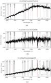 |
Fig. 3. Three examples of the cross-correlation results of Hydra spectra. The dashed lines and grey regions indicate the central wavelength and associated error of the labelled line. The red regions indicate those masked out during the cross-correlation process because of strong sky lines. (a) Good spectrum. (b) Low signal-to-noise. (c) Poor sky subtraction. |
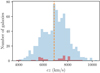 |
Fig. 4. Distribution of all redshifts (literature and new) within WCS footprint. The red represents the galaxies whose redshifts were obtained using Hydra/WIYN. |
2.2. Photometric data
Despite being an extremely well-studied cluster, there are no publicly available matched-aperture or total magnitude photometric catalogues that cover the entire region of Coma that we are interested in. It is important when comparing flux (or magnitude) measurements in different photometric bands that the measurements are determined in the same manner (i.e., matched apertures or model fits for total magnitudes). The overlapping sources at the centre of the cluster also provide a challenge to many aperture-based photometric pipelines. Our imaging data includes near- and far-ultraviolet (UV) data from the Galaxy Evolution Explorer (GALEX, Bianchi & GALEX Team 2000), five optical bands (ugriz) from SDSS (DR12 Alam et al. 2015), and the four mid-infrared bands (W1 − W4) from the Wide-field Infrared Survey Explorer (WISE, Wright et al. 2010). Frames from the 11 bands were mosaicked using SWARP (Bertin 2010) to create a single 2 × 2 deg2 image per band centred on the cluster, all with the same pixel scale (0.396″/px). We also created a pseudo B-band image from the SDSS g and i bands using the following relation from Cook et al. (2014) for conversion from SDSS to Johnsons magnitude:
 (1)
(1)
This relation was calibrated using galaxies in the Local Volume Legacy Survey (Dale et al. 2009). It should be noted that this pseudo B-band magnitude is only used to calculate the diameter (D25) of each galaxy at the 25 mag arcsec−2 isophote, which is required to estimate expected H I mass (see Sect. 4).
We followed the strategy used by Barden et al. (2012) in the GALAPAGOS pipeline to calculate magnitudes and other morphological properties for each galaxy for which we have a redshift measurement within the WCS footprint. For each galaxy we created a set of postage stamps that are then used to calculate properties such as magnitude and size. The modelling was done using GALFITM (Bamford et al. 2011), which is a modified version of GALFIT created by Peng et al. (2002, 2010). GALFITM is capable of modelling a source across multiple bands simultaneously. It is very sensitive to the initial parameters, and so we therefore calculated the initial values using source characterisation tools in photutils (an AstroPy package for photometry). We also used the photutils image segmentation feature to create masks for each band: any source not associated with our target is masked, with the exception of overlapping sources, which are modelled simultaneously using GALFITM. There are 23 galaxies for which the fit failed or was not possible because the galaxy is too faint (4 of these are known ultra-diffuse galaxies). These galaxies are still included in our spectroscopic sample as they come from spectroscopic surveys that targeted extremely faint dwarf galaxies (e.g., Chiboucas et al. 2010) or ultra-diffuse galaxies (e.g., Alabi et al. 2018).
An example of a single Coma galaxy modelled using a single Sersic profile by GALFITM is presented in Fig. 5. The Sersic profile, one of the most commonly used profiles for modelling galaxies of differing morphologies (Peng et al. 2010), is given by
![Mathematical equation: $$ \begin{aligned} I(r) = I_{\rm e} \exp \left[ -\kappa \left( \left(\frac{r}{r_{\rm e}}\right)^{1/n} - 1 \right) \right] , \end{aligned} $$](/articles/aa/full_html/2021/06/aa38738-20/aa38738-20-eq2.gif) (2)
(2)
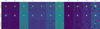 |
Fig. 5. Galaxy modelled with a single Sersic profile by GALFITM. The input data are shown in the top row, the model in the second row, and the residuals in the bottom row. The colour scale is set in every column such that each row has the same intensity. |
where Ie is the pixel intensity at the effective radius radius (re). The κ is tied to the value of n such that when n = 4 (making Eq. (2) consistent with a de Vaucouleurs profile), κ = 7.67 (Peng et al. 2010). Galaxies better described by an exponential profile have n = 1. During the model fitting process, we allow the model parameters to vary across the bands. The full catalogue of properties for Coma galaxies within the WCS footprint is given in Appendix C.
Stellar masses and star formation rates (SFRs) for the Coma galaxies are calculated following the method outlined in Cluver et al. (2014) and using a custom pipeline (Jarrett et al. 2013, 2019). The mass-to-light ratios for each galaxy are calculated from the WISE W1 − W2 colour using
 (3)
(3)
where LW1 is the W1 (3.4 μm) in-band luminosity of the galaxy relative to the Sun, and (W1 − W2) is the rest-frame colour (Cluver et al. 2014). The distribution of stellar masses for Coma is shown in panel a of Fig. 6.
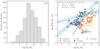 |
Fig. 6. Stellar mass and star formation distribution of Coma galaxies in the WCS footprint. Left: stellar mass distribution of Coma galaxies within the WCS footprint. Right: star formation rate as a function of stellar mass for the Coma galaxies. The 2σ upper limit on the star formation is shown for galaxies for which there is no detection in the W3 band; these are represented by the light grey points. The step function in the upper limits arises owing to a non-detection in W3 for low-mass galaxies and a non-detection after continuum subtraction in W3 for high-mass galaxies. Also shown for reference are fits to the star formation main sequence by Cluver et al. (2020), Popesso et al. (2019) and Saintonge et al. (2016). The black dashed line indicates the quench threshold (Cluver et al. 2020) below which galaxies are not considered to be actively star forming. |
As has been shown by Cluver et al. (2014, 2017), the W3 (12 μm) and W4 (23 μm) bands trace the interstellar medium (ISM) emission in galaxies and can thus be used to determine SFRs. The SFRs used in this work are calculated from the 12 μm luminosity (W3) relation determined by Cluver et al. (2017). The W3 flux measurements are separated into the contributions from polycyclic aromatic hydrocarbon (PAH) emission (which is related to the star formation activity) and a contribution from the stellar continuum (Cluver et al. 2017). Panel b of Fig. 6 shows the star formation as a function of stellar mass for the sample. Many of the Coma galaxies do not have a measured SFR, and therefore are presented as 2σ upper limits in Fig. 6. There is a step-distribution in the SFR upper limits, which arises as a result of the low-mass galaxies (M⋆ ≲ 109.5 M⊙) not detected in the W3 band. The higher-mass galaxies (M⋆ ≳ 109.5 M⊙) are detected, but the W3 flux is largely attributed to the stellar continuum that is removed prior to determining the SFR.
2.3. H I data
The blind, high-sensitivity and high-resolution WSRT H I observations from Molnar et al. (in prep.) provide an opportunity to study the gas content of Coma galaxies located well within the cluster environs, along with those on infall. Like most dense galaxy environments, Coma is well known for being H I deficient, and so we use the H I stacking method to probe the average H I content of groups of galaxies.
The WCS observed Coma in two overlapping 20 MHz bands (1369−1389 MHz and 1386−1406 MHz) and is comprised of 24 overlapping WSRT pointings of 1 × 12 h, making the effective integration owing to the overlap, 3 × 12 h per pointing. The final data cubes were created using the MIRIAD software package (Sault et al. 2011). Details about the data reduction are provided in Molnar et al. (in prep.). The two data cubes, together, cover approximately ∼5 deg2 and a velocity range of ∼3000−10 500 km s−1, however, there is a break in the velocity range of ∼24 km s−1 at the central cluster velocity of 6925 km s−1. The two H I cubes have a spatial resolution of 26.5 × 40.3 arcsec2 and a velocity resolution of 16.5 km s−1.
The WCS contains 39 galaxies for which there are direct H I detections, with H I masses greater than 4.4 × 10⁷ M⊙. The detections were identified using SoFiA (Serra et al. 2015) and confirmed by eye. Details on the source finding and discussion about the properties of the H I detections are provided in Molnar et al. (in prep.).
3. H I stacking method
The technique utilised in this study to probe the H I content of the galaxies in the Coma cluster is called H I stacking. This statistical technique has become popular to push the H I mass sensitivity below the observation limit. The technique is particularly useful to study the average H I properties of samples of galaxies that are predominantly not directly detected in H I. H I stacking has been successfully used to study the neutral gas content of galaxies in clusters and dense environments (e.g., Brown et al. 2017; Chengalur et al. 2001; Fabello et al. 2012; Jaffé et al. 2016; Lah et al. 2009; Verheijen et al. 2007).
H I stacking uses the optical redshift information for each galaxy to align the H I spectra. The aligned spectra are co-added to create an average spectrum with lower noise statistics than the individual spectra. In this study we make use of the publicly available H I Stacking Software (HISS; Healy et al. 2019)4 tool to perform all our stacking experiments.
For every galaxy with a redshift in our catalogue, we extract a spectrum from the H I data cubes. For galaxies where the B-band D25 is resolved by the beam, we extract the spectrum using an aperture with the semi-major axis determined from the galaxy diameter at the B-band 25th mag isophote (D25) (see Fig. A.1b). For galaxies unresolved by the beam, the corresponding H I spectra are extracted using an aperture the size of the beam (25″ × 40″) (see Fig. A.1a). Along with the target spectrum, for every galaxy, we also extract 25 “reference” spectra using the same aperture as the target spectrum. The bottom left panel of Figs. A.1a and b show the locations around the target from which the 25 reference spectra are extracted. These reference spectra are stacked in all our analyses in the same manner as the target galaxy spectra. For each target galaxy we extract background spectra from 25 offset positions around it. Taking as input a background spectrum from the same relative offset position around each target galaxy, we produce a background reference spectrum. Using all the offset positions results in 25 separate reference spectra per stacked target spectrum, with each reference spectrum containing the same number of stacked spectra as the target stack. Stacked reference spectra are used to aid in quantifying the signal in the main stacked spectrum. The average of the 25 stacked reference spectra for a well-calibrated dataset should be around zero (e.g., see the grey line in the panels of Fig. 10). From the spread of the 25 stacked reference spectra, we estimate the uncertainty on the quantity measured from the stacked target spectrum.
4. H I in Coma
4.1. H I–M⋆ scaling relation
The stellar mass (M⋆) to H I gas fraction (fH I, defined as the H I mass to stellar mass fraction) scaling relations (M⋆–fH I) are well characterised for galaxies in the field (e.g., Fabello et al. 2011; Brown et al. 2015; Healy et al. 2019), and have also been used to study the deficiency of H I in galaxies in different density environments including the Virgo cluster (e.g., Cortese et al. 2011; Fabello et al. 2012). However, given the small number of direct H I detections in Coma, there has been no study of the M⋆–fH I scaling relation as a method to probe the H I content of the cluster as a whole. In Fig. 7, we present the M⋆–fH I scaling relation for Coma.
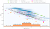 |
Fig. 7. Stellar mass (M⋆) to H I gas fraction (fH I) scaling relation for the Coma cluster. The individual 3σ upper limits for the Coma H I non-detections are represented by the grey down-pointing triangles, while the distribution of the individual H I detections is shown by the blue density plot. The pink diamond and orange down-pointing triangle symbols represent the stacking of all Coma galaxies and only non-detections, respectively. The pink diamonds show measurements from a detected stacked spectrum, and the orange triangles indicate the 3σ upper limit in the case of a non-detection in the stacked spectrum. The round light green symbols and green line represent the stacking of field galaxies by Healy et al. (2019) and Fabello et al. (2011), respectively; the dashed green line is an extrapolation of the Fabello et al. (2011) results. The individual fH I measurements (pink stars) for galaxies in the Ursa Major cluster are also shown for reference (Verheijen & Sancisi 2001). |
We separated the galaxies into samples by stellar mass (indicated by the histogram in Fig. 7) to probe the fH I–M⋆ scaling relation. Figure 7 shows the Coma direct H I detections in the blue distribution and the H I mass upper limits for the H I non-detections in grey down-pointing triangles. The H I mass upper limits are calculated using the noise from the individual spectra and an upper estimate on the W50 line width calculated using the r-band Tully–Fisher relation from Ponomareva et al. (2018). The scatter in the distribution of upper limits can also be attributed to the spread in the noise distribution of the WCS mosaic. Given the number of galaxies that are not detected in H I, we used the H I stacking technique to probe the H I content below the detection threshold.
Utilising the H I stacking technique, we were able to improve the sensitivity in the stacked spectrum by more than order of magnitude relative to the individual spectra. We stacked both detections and non-detections, as well as just non-detections. Despite the improved sensitivity of the stacked spectra, there are no detections in the stacked spectra corresponding to the sample with only non-detections; the stacked spectra for each stellar mass bin can be found in Figs. B.1 and B.2. The 3σ upper limits for the stacking results suggest that Coma galaxies on average have at least three orders of magnitude less gas than galaxies at the same stellar mass in the field (indicated by the round light green symbols Healy et al. 2019 and the dark green line Fabello et al. 2011). In comparison, galaxies in Ursa Major cluster (indicated by the pink stars from Bilimogga et al., in prep.) have just under an order of magnitude less gas than the field sample and an order of magnitude more than the results from stacking all Coma galaxies (magenta diamonds in Fig. 7).
Figure 7 shows that there is a large spread in H I gas fraction (fH I) values for the Coma galaxies, however looking at the average fH I values for all galaxies in the cluster (the pink diamonds in Fig. 7, which are measured from the stacked spectrum containing all individual detections and non-detections in the stellar mass bin), we note that on average, the Coma galaxies have fH I values that are between one and two orders of magnitude lower in each stellar mass bin than the field relations and other individual measurements from less dense environments. However, while the fH I–M⋆ scaling relation compares the H I mass to galaxies of similar stellar mass, galaxies of similar stellar mass but different morphology and size have different H I masses (Brown et al. 2015; Haynes & Giovanelli 1984; Healy et al. 2019). Thus, it is necessary to use a probe of the H I content that takes morphology and size into account.
4.2. H I deficiencies
The H I deficiency parameter (DEFH I, Haynes & Giovanelli 1984) is a useful quantity to understand how deficient a galaxy (or sample of galaxies) is compared to a field galaxy of the same size and morphology. It is defined as
 (4)
(4)
where MH I,exp is the expected H I mass, which is calculated using an optical–H I scaling relation that takes into account the morphology and size of the galaxy (Haynes & Giovanelli 1984; Denes et al. 2014).
The expected H I mass (MH I,exp) is derived from a log linear empirical relation, which is calibrated using field galaxies on varying morphologies and sizes (Haynes & Giovanelli 1984),
 (5)
(5)
where D25 is the diameter of the galaxy in the B-band at the 25th mag arcsec−2, and a and b are empirical constants dependent on the morphology of the galaxy (T type). The quantity h is taken to be 0.7 from H0 = 70 km s−1 Mpc−1. While there have been updates to the scaling relations used to estimate the H I mass of galaxies without using T types (e.g., Denes et al. 2014, 2016; Jones et al. 2018), the deficiencies presented in this work are calculated using T types.
The Coma galaxies have been separated into broad morphological bins: early-type galaxies, S0s, late-type galaxies, and irregular galaxies; galaxies for which we cannot reliably determine the classification are marked as unknown. The classifications were made by eye (by three adjudicators) using colour optical images from three different surveys (SDSS, PanSTARRS5, and DeCALS6) and g-band data observed using the Canada-France-Hawaii Telescope (Head et al. 2015). These classifications (where possible) have been cross-matched against the Galaxy Zoo database (Lintott et al. 2011) and the Third Reference Catalogue of Bright Galaxies (RC3; de Vaucouleurs et al. 1991) and are used to calculate the H I deficiency. The values used in Eq. (5) for the different morphological types are given in Table 1.
We calculated individual measures of the H I deficiency for every galaxy. For the galaxies for which there is no direct H I detection, we used the 3σ upper limit of the measured H I mass. This means that the corresponding H I deficiency measurement is a lower limit and the deficiency value is expected to increase in the case of a better sensitivity spectrum.
Denes et al. (2014) used data from the H I Parkes All Sky Survey (HIPASS; Meyer et al. 2004) to map the global H I deficiency across the southern sky. They found that regions that contained an over-density of H I deficient galaxies correlated with known dense galaxy regions. The known galaxy clusters in the southern sky have an average H I deficiency that lies between 0.5 < DEFH I < 2. For the many Coma galaxies where there is no direct H I detection, we measured a lower limit on the H I deficiency. These lower limits for the DEFH I of the Coma galaxies (grey triangles) are predominantly between 0.5 < DEFH I < 2, which indicates that Coma is at least as deficient as the clusters covered in the Denes et al. (2014) sample.
For a sample of 18 clusters, Solanes et al. (2001) studied the H I deficiency of spiral galaxies residing inside one Abell radius compared to those outside. They compare the fraction of H I deficient spirals against different cluster properties. Coma is consistent in the total number of spiral galaxies given its X-ray luminosity, however it is an outlier in the number of H I deficient spirals for its mass, Abell richness, and total number of spiral galaxies. Gavazzi et al. (2006) did a more detailed study on the radial pattern of H I deficiency across the Coma Supercluster. However, like Solanes et al. (2001), the Gavazzi et al. (2006) work only focusses on the late-type galaxies across the cluster.
In this work, we revisit the work by Gavazzi et al. (2006), however we focus on H I non-detections, which cover all galaxy morphologies across the cluster. To calculate the average DEFH I for the H I non-detected galaxies, we used the H I stacking technique to stack the galaxies in annuli with increasing radius from the cluster centre, scaling each input spectrum by the expected H I mass of the galaxy (see Fabello et al. 2011, Eq. (3.5)) for same technique but for H I gas fractions). While there are no clear detections in the stacked spectra (see Figs. B.3–B.5), we push the lower limits higher than the individual spectra (see the black triangles in Fig. 8). These results indicate a bi-modality in the H I content of the Coma galaxies – we either detect H I or the galaxies contain on average at least ∼10−100 times less H I than their field counterparts. This suggests an extremely fast and efficient quenching mechanism.
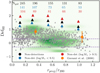 |
Fig. 8. H I deficiency of the Coma galaxies as a function of projected radius from the cluster centre. The individual H I deficiency measurements for the Coma galaxies are represented by the green shaded distribution for the H I detections and grey triangles for the lower limits on the H I non-detections. The average H I deficiencies for late-type Coma galaxies from Gavazzi et al. (2006) are shown in orange. The black, blue, and red triangles represent the lower limits from stacking the non-detections in annuli in three samples: all non-detections, log M⋆ < 9.5, and log M⋆ > 9.5, respectively. The horizontal dashed purple lines set the limit on DEFH I values that indicate a galaxy is H I-normal. |
Oman & Hudson (2016) show using N-body simulations of clusters that the time for quenching low-mass galaxies is longer than that of high-mass galaxies. We thus separated the non-detections by stellar mass into a high stellar mass sample (M⋆ > 109.5 M⊙, represented by the red symbols in Fig. 8) and a low stellar mass sample (M⋆ < 109.5 M⊙, represented by the blue symbols in Fig. 8). We choose this stellar mass as it is the so-called “gas-richness” threshold (Kannappan et al. 2013): galaxies below this threshold are typically H I gas-rich, while galaxies above this threshold are typically H I gas-poor. For both subsamples, there are no detections in the stacked spectra at any radius. These results set lower limits on the average H I deficiencies for the low- and high-stellar mass populations and we are therefore unable to compare to radial trends in other clusters (e.g., Solanes et al. 2001; Gavazzi et al. 2006) or to quenching times for different mass samples (Oman & Hudson 2016) with these data.
4.3. H I stacking in and around the cluster
In this section we explore the average H I content of the Coma galaxies. The focus is the total galaxy sample, including galaxies without direct detections. The direct H I detections are studied in detail in Molnar et al. (in prep.). Figure 9 shows the line-of-sight velocity relative to the cluster (Δvr/σcl; σcl is the cluster velocity dispersion, 1180 km s−1) as a function of the projected radius from the centre of the cluster (rproj/r200, where r200 = 1.8 Mpc is the radius at 200 ρcrit; Gavazzi et al. 2009); the data points are coloured by their g − r colour. The escape velocities for the cluster are determined using the prescription outlined in Jaffé et al. (2015) assuming a concentration index (c) of 5, and M200 = 5.1 × 10¹⁴ M⊙ (Gavazzi et al. 2009). We refer to Fig. 9 as the phase-space diagram throughout this work.
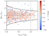 |
Fig. 9. Phase-space diagram for Coma. The black dashed lines represent the escape velocity for Coma, calculated using a concentration index (c) of 5, M200 = 5.1 × 10¹⁴ M⊙ and r200 = 1.8 Mpc (Gavazzi et al. 2009). Galaxies inside the escape velocity ‘trumpet’ are considered to be within the cluster, while galaxies on the outside edge of the trumpet are considered to be falling into the cluster. The light grey shaded cone represents the virialised zone (Oman et al. 2013). The g − r colour of each galaxy is given by the colour scale in colourbar. |
We separate the Coma galaxies into four samples, by the regions in the phase-space diagram in Fig. 9: (1) virialised cone; (2) inside r200 which includes all galaxies with rproj < r200 and within the escape velocity “trumpet”, but excludes the galaxies in the virialised cone; (3) outside trumpet, which includes all galaxies with rproj < r200, but line-of-sight velocities that place them outside of the escape velocity trumpet; and (4) outside r200 (all galaxies with rproj > r200). The four samples are further separated by g − r colour. Galaxies with g − r < 0.6 are considered to be blue, and those with g − r > 0.6 are considered to be red. For Coma, g − r = 0.6 provides a good separation between the red sequence and the star-forming blue cloud. The stacked spectra for each sample (with direct H I detections excluded) are presented in Fig. 10. It should be acknowledged that the four samples (virialised zone, inside r200, outside trumpet, and outside r200) contain interlopers due to projection effects especially along the line-of-sight velocity. These projection effects most likely affect the three samples contained within the r200 radius of the cluster.
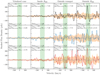 |
Fig. 10. Stacked spectra for all (top row), blue (middle row), and red (bottom row) H I non-detections in different regions of the cluster. The average stacked spectrum in each panel is indicated by the solid black, blue, and red lines. The average stacked reference spectrum is represented by the solid grey line. The green band indicates the velocity range cz ± 200 km s−1 over which H I emission is expected to be seen. Only the sample of galaxies outside the r200 (right-most column) of the cluster appear to contain detectable H I. |
In Fig. 10 we compare the average H I content of the galaxies for which there are no direct H I detections for the three different regions of the cluster. We also separate the galaxies by colour; the resulting average spectra for the blue and red galaxies in each region are shown in the middle and bottom rows of Fig. 10. The stacked spectra are smoothed after stacking to a velocity resolution of 40 km s−1 to improve the signal-to-noise ratio (S/N). We also stack the 25 reference spectra (see Sect. 3) using the same scheme as the target spectra. From the 25 stacked reference spectra, we create an average reference spectrum represented by the grey spectra in Fig. 10. Also shown in Fig. 10 is the variance of the 25 stacked reference spectra; this is represented by the orange band around the grey line. The comparison between the average reference spectrum, where we do not expect to see a signal, and the stacked target spectrum provides confidence that any signal visible in the target spectrum is real. We consider stacked spectra with a signal in the region v = 0 ± 200 km s−1 that has S/N = 3.5 to be marginally detected. We feel confident using a S/N = 3.5 since there is no corresponding signal in the reference spectrum.
Only the sample of galaxies outside r200 shows a possible detection in all three colour samples. Even though both the red and blue samples have roughly the same average H I mass (⟨MH I⟩), it should be noted that the lower limits on the average H I deficiency (⟨DEFH I⟩), which is shown in the bottom left corner of each panel, show the red galaxies to be more H I deficient than the blue galaxies. Despite both the blue and red samples showing lower limits for the H I deficiency, the two samples have similar number of galaxies meaning that the stacked spectra have similar sensitivities making their limits comparable. The difference between the DEFH I for the two samples is not unexpected as red galaxies are well known for being more gas poor than blue galaxies. Unlike what is found by Jaffé et al. (2016) for Abell 963, none of the samples show any possible detections within the r200; however these authors also do not detect a signal for their red galaxies outside the r200, which we do.
Simulations have shown that quenching begins after some delay time once a galaxy has crossed 2.5 vvir (for reference, r200 ∼ 0.73 rvir, Oman & Hudson 2016) with higher-mass galaxies affected slightly more quickly than lower-mass galaxies (Oman & Hudson 2016), however once quenching has begun, the time taken for the galaxies to transition from a field-like galaxy to one fully processed by the cluster is very short. Indeed, less than 10 of our galaxies outside r200 have measurable SFRs, and most of those are below the star-forming main sequence (see panel b of Fig. 6 for galaxies with 7 < log M⋆/M⊙ < 9.5).
Gavazzi et al. (2006) show on average Coma galaxies at r > 5 Mpc, which is beyond 2 rvir, are H I normal. We have shown in the previous section, on average, that our Coma galaxies are (at a lower limit) at least 10–100 times more H I deficient than their field counterparts. If we assume that galaxies that are accreted onto the cluster are H I normal and on the star-forming main sequence when they cross 2.5 rvir, the processes driving the removal of H I in galaxies as they fall into the cluster must be very quick and have a strong influence beyond rvir. In Sect. 6.4 we also compare the average H I content between the Coma galaxies in groups or substructure to those that are not associated with any groups.
5. Finding substructure in Coma
Substructure, defined as structure kinematically distinct from the parent halo, is a natural consequence of a hierarchical universe (Hou et al. 2012). As discussed in the introduction, there are many different methods that can identify substructure within a galaxy cluster (e.g., Adami et al. 2005; Dressler 1980; Jaffé et al. 2013; Neumann et al. 2003). We are interested in how the average H I gas content may change in groups or substructure with different morphologies or possible infall times across the cluster.
To identify these groups/substructure, we chose to use the DS test to identify groups that are kinematically distinct from the cluster. Dressler & Shectman (1988b) applied their test for kinematic deviations to look for substructure in a number of Abell clusters (including Coma). Their conclusion regarding Coma was that there was no substructure within the cluster. Since Dressler (1980), there have been many targeted and blind spectroscopic surveys of the Coma cluster and subsequent studies of Coma have found significant substructure (e.g., Adami et al. 2005; Colless & Dunn 1996). To detect substructure, one needs ∼1000 redshifts in a ∼1 Mpc region (Adami et al. 2005). We apply the DS test, given by
![Mathematical equation: $$ \begin{aligned} \delta _i^2 = \left( \frac{N_{\rm nn} + 1}{\sigma _{\rm cl}^2} \right) \left[ ( \bar{{ v}}_{\rm local}^i - \bar{{ v}}_{\rm cl})^2 + (\sigma _{\rm local}^2 - \sigma _{\rm cl}^2) \right], \end{aligned} $$](/articles/aa/full_html/2021/06/aa38738-20/aa38738-20-eq6.gif) (6)
(6)
to our redshift catalogue. We used nearest neighbour (Nnn) values in increments of 5 from 5–30 with a velocity dispersion (σcl) of 1180 km s−1 and a cluster velocity (vcl) of 6925 km s−1. Figure A.2 shows the results of the DS Test for Nnn = 25. Using similar plots for all the Nnn values, and two independent judges, we identified groups where there are large overlapping circles (which represent large δi values) of similar colour representing similar velocity values. Using the Nnn = 25 as a reference, galaxies were assigned to groups using a combination of the different Nnn runs.
Within the WCS H I data footprint, we find 15 distinct groups. These groups stand out across the six iterations of the DS test, and are highlighted by the different colours in Fig. 11. The properties of the 15 groups are given in Table 2. Despite the difference in the method of identifying substructure, we find some overlap between our groups and those identified by Adami et al. (2005), who use a hierarchical clustering algorithm (see Serna & Gerbal 1996) which uses a measure of the binding energy to find groups of galaxies that are bound in substructure. Of the 17 groups Adami et al. (2005) found, 14 are within the WCS footprint and seven correspond to groups that we found using the DS Test. The groups overlapping between our work and Adami et al. (2005) are S1, S2, S6, and S11 (combined into one group at the core of the cluster), S8, S9, and S15.
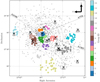 |
Fig. 11. Substructure in the WCS footprint. The 15 identified groups are shown in different colours. The background grey contours represent the X-ray emission measured by ROSAT in 0.4−2.4 keV. The dashed grey lines indicate the direction to nearby clusters connected to Coma. The groups identified by Adami et al. (2005) are labelled and denoted by black crosses. |
Details of the 15 groups found within the Coma cluster using the DS test.
6. Identified substructures
6.1. Core substructures
In the core of the cluster (see Fig. 11), we identified two groups (groups S1 and S2) around the two cD galaxies (NGC 4874 and NGC 4889) and another two groups surrounding the two central groups: S3 and S5. There is much discussion in the literature surrounding the centre of the Coma cluster. A commonly accepted scenario is that the two cD galaxies eventually merge (e.g., Colless & Dunn 1996; Adami et al. 2005).
Using the hierarchical clustering method to developed by Serna & Gerbal (1996) to identify substructure, Adami et al. (2005) found one group (G1) in the central region of the cluster. These authors later note that with X-ray analysis there are two distinct peaks in the X-ray corresponding to the two galaxies. They postulate that these two groups are in the process of colliding: S1, the larger of the two groups with 27 members, has a mean velocity of 7699 km s−1, and S2 (with 18 members) has a mean velocity of 6113 km s−1. Both the groups have velocity dispersions that are of the order of ∼900 km s−1 (see Table 2 for more details).
Located immediately north of S1 and S2 (see Fig. 12), S3 contains 14 members. The smallest group containing only six galaxies, S5 is located to the south-west of S1. Both the S3 and S5 groups are dominated by early-type and S0 galaxies. None of these groups (S1, S2, S3, or S5) show a detection of H I in their stacked spectra (see Fig. B.6), however given the gas removal processes at play in cluster centres, this is unsurprising. The measured upper limits on the H I mass and lower limits on the H I deficiency for the groups can be found in Table 2, and the corresponding stacked spectra in Appendix B.
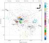 |
Fig. 12. Fifteen identified groups within the WCS footprint. The contours (taken from Adami et al. 2005, Fig. 4) represent the X-ray excess found by Neumann et al. (2003). |
6.2. Groups coincident with excess X-ray emission
6.2.1. South-west structure
Using X-ray observations by XMM-Newton, Neumann et al. (2003) studied the dynamical structure within Coma. They fit an elliptical beta model to the X-ray emission where any residuals from this fit may indicate structure within the cluster. Figure 2 in Neumann et al. (2003) shows that there is X-ray emission not explained by the beta model. Neumann et al. (2003) also found a number of bright galaxies coincident with the peaks in this excess emission. Adami et al. (2005) compared the groups that they found to the excess X-ray emission maps from Neumann et al. (2003), and found a number of overlaps. We used the excess X-ray contours from Adami et al. (2005, Fig. 4) to compare to the location of our groups. Figure 12 shows the isocontours residual X-ray emission along with the location of our groups. Figure 12 shows that groups S4, S6, S8, S9, S10 (this group is slightly offset from the X-ray), and S11 are coincident with X-ray emission.
Of the groups we identified that are coincident with X-ray emission, S11 is perhaps the most well studied (e.g., Colless & Dunn 1996; Neumann et al. 2001; Akamatsu et al. 2013; Burns et al. 1994; Lyskova et al. 2019; Beijersbergen 2003). The S11 group is located to the south-west of the cluster core and is home to NGC 4839. Previously, Beijersbergen (2003) found a group of 18 galaxies within 0.15° of NGC 4839, and using data from their blind WSRT H I survey of the cluster, calculated for the group, an average H I mass (MH I) 3σ upper limit to be ⟨MH I⟩ < 7.55 × 10⁸ M⊙. Within the same radius, we found 26 galaxies, however using the DS test we found 36 galaxies associated with this group. Our average 3σ mass limit is ⟨MH I⟩ < 2.29 × 10⁷ M⊙. Many groups have studied this collection of galaxies in an effort to understand if it is still on first infall (e.g., Colless & Dunn 1996; Neumann et al. 2001; Akamatsu et al. 2013), or has already passed through the centre of the cluster (e.g., Burns et al. 1994; Lyskova et al. 2019).
Lyskova et al. (2019) show using smooth particle hydrodynamical simulations that a post-merger scenario, in which the group has already passed around the centre of the cluster, explains the observed X-ray emission better than the pre-merger scenario where this group is on first infall. In the post-merger scenario, Lyskova et al. (2019) postulate that S11 entered the cluster from a filament on the north-east side of the cluster. Malavasi et al. (2020) use the DisPerSE algorithm to identify filaments connecting to Coma, and while they identify three such filaments (including one joining to the north-east of the cluster), they do not identify the filament known as the “Great Wall” to the south-west of Coma, which connects the cluster to Abell 1367. It is the “Great wall” filament that S11 is thought to be accreted from (Colless & Dunn 1996; Akamatsu et al. 2013). From our results, we cannot conclude whether these groups are on first infall, or have already passed through the cluster. However, our results indicate that this group is extremely H I deficient and contains an evolved population of galaxies; this supports the post-merger scenario, but also the first infall scenario under the assumption that this group has been pre-processed. Recent work by Salerno et al. (2020) has shown that filaments can be very effective at quenching star formation. Nevertheless, the question whether the NGC 4839 (S11) group is on first infall or has already passed through the cluster, remains open.
6.2.2. South-eastern structure
Neumann et al. (2003) identified X-ray substructure to the south-east of the core of the cluster (see S4, S8, and S9 in Fig. 12). Neumann et al. (2003) attributed this X-ray over-density to emission from the intra-group medium of one group of galaxies containing NGC 4911 and NGC 4921. They attributed the bending in the structure due to projection effects by assuming that the direction of the structure motion is to the east with NGC 4921 at the head. They also concluded that NGC 4911 and NGC 4921 are gravitationally bound because they have similar velocities. We do not find these two galaxies to be part of the same group, which can largely be attributed to the differences in their velocities (∼2000 km s−1). The velocity we used for NGC 4926 is taken from SDSS DR13. The SDSS DR13 measurement is in good agreement with other optical and H I redshift measurements of this galaxy (e.g., Dressler & Shectman 1988a; de Vaucouleurs et al. 1991; Zabludoff et al. 1993; Haynes et al. 1997; Bravo-Alfaro et al. 2000), including the H I measurement from the WCS. Adami et al. (2005) also found NGC 4911 and NGC 4926 to be part of different groups and note that the velocity quoted by Neumann et al. (2003) is incorrect.
We identified three groups (S4, S8, and S9) coincident with this X-ray substructure; S8 and S9 have been previously identified by Adami et al. (2005) as G4 and G7, respectively. The S8 group contains NGC 4911, which appears to be spatially coincident with the peak of the X-ray emission (Adami et al. 2005; Neumann et al. 2003). If the X-ray is associated with these groups, the fact that it is still detectable implies that the groups have not yet passed through the cluster (Adami et al. 2005). However the X-ray emission shows no sign of shock heated gas, which is a signature of radial infall, thus Adami et al. (2005) argued that it is more likely that these groups are on a spiral infall trajectory. Of the three groups, S4 and S8 have mean velocities that are higher than the cluster velocity; S4 and S8 also contain a number of late-type and irregular galaxies (in addition to the E and S0 galaxies), whereas S9 is dominated by early-type galaxies (E or S0) and has only one late-type galaxy (see Table 2). Both S4 and S8 are on average extremely H I deficient (⟨DEFH I⟩ > 1, see Table 2), thus it is possible that the galaxies have been stripped of their H I, a process that can occur extremely rapidly after crossing into the cluster (∼2.5 rvir), but the presence of the bluer galaxies may indicate that they have yet to transition across the ‘green valley’ (Oman & Hudson 2016). Dominated by an older population of galaxies, S9 has a mean velocity of 6498 km s−1, which is similar to that cluster velocity and could indicate that it is moving in the plane of the sky. The presence of one H I detection in this group would imply that it could also be a recent infall, however given the difference in mean velocities from S4 and S8, it is unlikely to have followed the same trajectory.
6.2.3. Western filament
The last major X-ray residual is the western filament which is aligned north-south, extending roughly a megaparsec north from NGC 4839. Neumann et al. (2003) discussed possible origins of this structure: the change in X-ray temperature between the western filament and the centre of the cluster suggests that it could be due to heating from compression or shock waves during the infall of a structure onto the core of the cluster. They also discussed the possibility that the two X-ray maxima in the filament are due to a galaxy group that was broken up on infall; they discount the possibility of two groups falling in to the cluster at the same time. However, Neumann et al. (2003) did not find any galaxy over-densities associated with the filament.
Adami et al. (2005) found two groups coincident with the western filament: G12 and G14 (see Fig. 11). We also found two groups coincident with the filament: S6 and S10 (see Fig. 12). Located about half way up the filament, S6 is coincident with G14 found by Adami et al. (2005). Our other group that is coincident with the filament, S10, is located at the northern most part of the structure.
Both S6 and S10 lie on lines that connect Coma to other clusters: S6 on the line connecting to Abell 1367, and S10 on the line connecting to Abell 779 (see Fig. 12). Both of these groups are dominated by early-type and S0 galaxies, however, S10 contains one direct H I detection that dominates the stacked spectrum (see Fig. B.6). The S10 group has a higher average velocity (cz = 8355 km s−1) than Coma which could indicate that it is falling in from the filament connected to Abell 779. The average velocity of S6 is similar to Coma, which like S9, could either indicate that the group is moving slowly or in the plane of the sky.
6.3. Groups near the outskirts
There are four groups that can be considered on the outskirts: S12, S13, S14, and S15. Of these four groups, only S15 had been previously identified by Adami et al. (2005) as G5. Adami et al. (2005) identified five other groups on the outskirts of the cluster that we do not identify in this work. It should be noted that two of those groups are outside our H I dataset and the other two are on the edge. Despite using a galaxy catalogue that covered a larger area than our H I dataset, we only identified groups for which we had H I data. The one group contained within our H I dataset by Adami et al. (2005) that we did not find, G11, is located around α = 12h57m δ = 27° 00′. It is clear from Fig. A.2, which shows the results of the DS test, that there are no overlapping large circles of similar colour. Given that our redshift catalogue has more redshifts than Adami et al. (2005), in particular in that region owing to our observing campaign with WIYN (see Sect. 2.1.2), it is possible that with the smaller number of redshifts, G11 was artificially highlighted.
The S13 group has a diverse population of galaxies and contains the highest number of direct H I detections, while the other three groups (S12, S14, and S15) are dominated by older early-type or S0 galaxies with no direct H I detections. Both S14 and S15 lie on lines to other clusters (Abell 2199 and Abell 1367, respectively) and have similar velocities to the cluster indicating slow movement or a velocity vector in the plane of the sky. If S14 is being accreted onto Coma, then the average H I deficiency of the group and the evolved galaxy morphologies could indicate that this group underwent advanced evolutionary processes prior to being accreted. The high average velocity of S13 (cz = 7351 km s−1) could indicate that it is falling into Coma from the foreground, this is supported by the fact that this group is not in line with any of the known filaments connecting to Coma. Given that S13 also contains so many direct detections, this also may suggest that it is being accreted from a low-density environment.
6.4. H I in substructure versus the cluster
We explore the H I content of the Coma galaxies in substructure compared to Coma galaxies not in substructure. We separate the Coma galaxies into 0.4 Mpc annuli increasing from the cluster centre. The 15 substructures are also separated into the different annuli: S1–S5 (0−0.4 Mpc), S6–S11 (0.4−0.8 Mpc), and S12–S15 (> 1.2 Mpc). Figure 13 shows the stacked spectra for galaxies in groups in the different annuli (top row) as well as galaxies not in groups (bottom row). There are no possible detections in any of the stacked spectra in Fig. 13 with the exception of the galaxies with r > 1.2 Mpc. This is perhaps not surprising as we did not take into account the velocity of the galaxies when separating them into the different annuli. It is possible that there are infalling galaxies in the two innermost annuli; however, this inner region is typically dominated by the oldest members of the cluster.
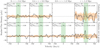 |
Fig. 13. Stacked spectra for galaxies in groups (top row), and galaxies not in groups (bottom row) separated into different annuli from the cluster centre. The average stacked spectrum in each panel is indicated by a solid black line. The average stacked reference spectrum is represented by a solid grey line, with the variance of 25 stacked reference spectra surrounding the average reference spectrum in orange. The green band is the velocity range cz ± 200 km s−1 over which the H I emission is expected to be seen. |
In order to explore the difference in H I content between galaxies not associated with any substructure and those that reside in substructure in the different regions of the cluster, we separated the two groups of galaxies into three bins loosely based on the regions of the phase–space diagram (Fig. 9). The galaxies and substructures that reside predominantly in the virialised cone are assigned to the ‘virialised bin’; galaxies/substructures inside r200 are assigned to the ‘inside cluster’ bin, and the remaining galaxies/substructures, which predominantly have rproj > r200, are assigned to the ‘recent infalls’. The resulting stacked profiles for the six samples are presented in Fig. 14. The top panel of Fig. 14 shows the stacked spectra from the galaxies in substructure and the bottom panel shows the stacked spectra from the galaxies not associated with any substructure. As with all the previous stacking, we only examine the galaxies for which there are no direct H I detections.
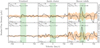 |
Fig. 14. Stacked spectra for galaxies in groups (top row), and galaxies not in groups (bottom row) separated into different regions in the cluster. The average stacked spectrum in each panel is indicated by a solid black line. The average stacked reference spectrum is represented by a solid grey line, with the variance of 25 stacked reference spectra surrounding the average reference spectrum in orange. The green band is the velocity range cz ± 200 km s−1 over which the H I emission is expected to be seen. |
We note detections in the stacked spectra for the ‘recent infalls’ samples, both for galaxies in groups and galaxies not associated with any substructure (right-most panels of Fig. 14). It is not unexpected that only the ‘recent infalls’ show detections in the stacked spectrum. The average H I deficiency measurement for each sample is given in the bottom left corner of each panel in Fig. 14. It is interesting to note that while the two samples (galaxies within substructure and galaxies not in substructure) have similar average H I masses, they differ in average H I deficiencies. Galaxies in groups have a lower limit on the average H I deficiency of ⟨DEFH I⟩ > 1.47, while the non-group galaxies have an average H I deficiency of ⟨DEFH I⟩ = 1.05 ± 0.56. The galaxy size, stellar mass, and colour distribution for both samples is similar, and while the ⟨DEFH I⟩ measurements indicate that both samples are H I deficient, the fact that we can only measure a lower limit on the average H I deficiency for the group galaxies suggests that they are more deficient than the non-group galaxies for which we can measure an average H I deficiency. This could indicate that the gas removal process is more efficient for the group galaxies.
7. Summary
In this work we have aimed to study the average H I content and morphologies of galaxies in the substructure of the Coma cluster. We collated a large catalogue of redshifts for the Coma cluster, including 59 new redshifts that we observed with the multi-object spectrometer, Hydra, at WIYN. Using the newly compiled catalogue, we applied the DS test to find substructure within the cluster. Fifteen substructures were found, of which three had not been previously identified.
The WCS provided high-resolution and high-sensitivity H I data that covered both the cluster core and the NGC 4839 group to the south-west. However, with only 39 direct H I detections out of the 850 galaxies that lie within the WCS footprint, we needed an alternate method to study the H I content of the galaxies in the different groups. The H I stacking technique enabled us to probe the average H I content of samples of galaxies.
Using the H I stacking technique, we are able to probe ∼1–2 orders of magnitude lower in H I mass. Despite this improvement in sensitivity, for many of the stacked samples there is no detection in the stacked spectrum. The H I gas fraction to stellar mass relation as well as a study of H I deficiency indicates that Coma galaxies are at least 50 times more H I deficient than their field counterparts. The bi-modality in the H I content, where galaxies either have detectable H I content or contain orders of magnitude less H I than expected, supports the theories that favour extremely rapid quenching and gas removal mechanisms.
Given the effectiveness of gas removal processes increases closer to the centre of the cluster, we expect to see the average H I content increase with distance from the cluster centre. For most samples of galaxies inside the cluster r200, there is no H I detectable in the stacked spectra, however we do detect H I in both blue and red galaxies outside the r200. When we separate the outer galaxies into those that are in groups versus those not in groups, both samples show detections in the ‘recent infall’ galaxies (see Fig. 14). The average H I masses for the two samples are similar, however we note that the average H I deficiency for the group galaxies is not detected at a lower limit that is higher than the measured average H I deficiency of the non-group galaxies, implying that the group galaxies are more H I deficient.
The WIYN Observatory is a joint facility of the University of Wisconsin-Madison, Indiana University, the National Optical Astronomy Observatory, and the University of Missouri.
IRAF is distributed by the National Optical Astronomy Observatory, which is operated by the Association of Universities for Research in Astronomy (AURA) under a cooperative agreement with the National Science Foundation.
Panoramic Survey Telescope and Rapid Response System (Chambers et al. 2016).
The Dark Energy Camera Legacy Survey (Dey et al. 2019).
Acknowledgments
We thank the anonymous referee for their comments that have improved this work. This project has received funding from the European Research Council (ERC) under the European Union’s Horizon 2020 research and innovation programme (grant agreement no. 679627; project name FORNAX). JH acknowledges research funding from the South African Radio Astronomy Observatory. We thank R. Healy for useful comments that improved the readability. Based on observations at Kitt Peak National Observatory, National Optical Astronomy Observatory (NOAO Prop. ID: 2017A-0356; PI: J. Healy), which is operated by the Association of Universities for Research in Astronomy (AURA) under a cooperative agreement with the National Science Foundation. JMvdH acknowledges support from the European Research Council under the European Union’s Seventh Framework Programme (FP/2007-2013)/ERC Grant Agreement no. 291531 (HIStoryNU). MV acknowledges support by the Netherlands Foundation for Scientific Research (NWO) through VICI grant 016.130.338. Funding for the Sloan Digital Sky Survey IV has been provided by the Alfred P. Sloan Foundation, the U.S. Department of Energy Office of Science, and the Participating Institutions. SDSS acknowledges support and resources from the Center for High-Performance Computing at the University of Utah. The SDSS web site is www.sdss.org. SDSS is managed by the Astrophysical Research Consortium for the Participating Institutions of the SDSS Collaboration including the Brazilian Participation Group, the Carnegie Institution for Science, Carnegie Mellon University, the Chilean Participation Group, the French Participation Group, Harvard-Smithsonian Center for Astrophysics, Instituto de Astrofísica de Canarias, The Johns Hopkins University, Kavli Institute for the Physics and Mathematics of the Universe (IPMU)/University of Tokyo, the Korean Participation Group, Lawrence Berkeley National Laboratory, Leibniz Institut für Astrophysik Potsdam (AIP), Max-Planck-Institut für Astronomie (MPIA Heidelberg), Max-Planck-Institut für Astrophysik (MPA Garching), Max-Planck-Institut für Extraterrestrische Physik (MPE), National Astronomical Observatories of China, New Mexico State University, New York University, University of Notre Dame, Observatário Nacional/MCTI, The Ohio State University, Pennsylvania State University, Shanghai Astronomical Observatory, United Kingdom Participation Group, Universidad Nacional Autánoma de México, University of Arizona, University of Colorado Boulder, University of Oxford, University of Portsmouth, University of Utah, University of Virginia, University of Washington, University of Wisconsin, Vanderbilt University, and Yale University. This publication makes use of data products from the Wide-field Infrared Survey Explorer, which is a joint project of the University of California, Los Angeles, and the Jet Propulsion Laboratory/California Institute of Technology, funded by the National Aeronautics and Space Administration.
References
- Abramson, A., Kenney, J. D., Crowl, H. H., et al. 2011, AJ, 141, 164 [Google Scholar]
- Adami, C., Biviano, A., Durret, F., & Mazure, A. 2005, A&A, 443, 17 [NASA ADS] [CrossRef] [EDP Sciences] [Google Scholar]
- Aguerri, J. A. L. 2012, Adv. Astron., 2012, 35 [Google Scholar]
- Akamatsu, H., Inoue, S., Sato, T., et al. 2013, PASJ, 65, 89 [NASA ADS] [Google Scholar]
- Alabi, A., Ferré-Mateu, A., Romanowsky, A. J., et al. 2018, MNRAS, 479, 3308 [Google Scholar]
- Alam, S., Albareti, F. D., Prieto, C. A., et al. 2015, ApJS, 219, 12 [NASA ADS] [CrossRef] [Google Scholar]
- Albareti, F. D., Prieto, C. A., Almeida, A., et al. 2017, ApJS, 233, 27 [Google Scholar]
- Andrade-Santos, F., Nulsen, P. E., Kraft, R. P., et al. 2013, ApJ, 766, 107 [Google Scholar]
- Balogh, M. L., & Morris, S. L. 2000, MNRAS, 318, 703 [Google Scholar]
- Balogh, M. L., Navarro, J. F., & Morris, S. L. 2000, ApJ, 540, 113 [Google Scholar]
- Bamford, S. P., Häußler, B., Rojas, A., & Borch, A. 2011, in Astronomical Data Analysis Software and Systems XX, eds. I. N. Evans, A. Accomazzi, D. J. Mink, & A. H. Rots (San Fransisco: ASP), 442, 479 [NASA ADS] [Google Scholar]
- Barden, M., Häußler, B., Peng, C. Y., McIntosh, D. H., & Guo, Y. 2012, MNRAS, 422, 449 [NASA ADS] [CrossRef] [Google Scholar]
- Beijersbergen, M. 2003, PhD Thesis, University of Groningen [Google Scholar]
- Bertin, E. 2010, Astrophysics Source Code Library [record ascl:1010.068] [Google Scholar]
- Bianchi, L., & GALEX Team 2000, Mem. Soc. Astron. It., 71, 1117 [Google Scholar]
- Bird, C. M. 1994, AJ, 107, 1637 [NASA ADS] [CrossRef] [Google Scholar]
- Biviano, A., Durret, F., Gerbal, D., et al. 1996, A&A, 311, 95 [NASA ADS] [Google Scholar]
- Boselli, A., & Gavazzi, G. 2009, A&A, 508, 201 [NASA ADS] [CrossRef] [EDP Sciences] [Google Scholar]
- Bravo-Alfaro, H., Cayatte, V., van Gorkom, J. H., & Balkowski, C. 2000, AJ, 119, 580 [Google Scholar]
- Bravo-Alfaro, H., Cayatte, V., van Gorkom, J. H., & Balkowski, C. 2001, A&A, 379, 347 [NASA ADS] [CrossRef] [EDP Sciences] [Google Scholar]
- Brown, T., Catinella, B., Cortese, L., et al. 2015, MNRAS, 452, 2479 [NASA ADS] [CrossRef] [Google Scholar]
- Brown, T., Catinella, B., Cortese, L., et al. 2017, MNRAS, 466, 1275 [NASA ADS] [CrossRef] [Google Scholar]
- Burns, J. O., Roettiger, K., Ledlow, M., & Klypin, A. 1994, ApJ, 427, L87 [Google Scholar]
- Caldwell, N., Rose, J. A., Sharples, R. M., Ellis, R. S., & Bower, R. G. 1993, AJ, 106, 473 [Google Scholar]
- Carter, D., Goudfrooij, P., Mobasher, B., et al. 2008, ApJS, 176, 424 [Google Scholar]
- Castander, F. J., Nichol, R. C., Merrelli, A., et al. 2001, AJ, 121, 2331 [Google Scholar]
- Chambers, K. C., Magnier, E. A., Metcalfe, N., et al. 2016, ArXiv e-prints [arXiv:1612.05560] [Google Scholar]
- Chengalur, J. N., Braun, R., & Wieringa, M. 2001, A&A, 372, 768 [EDP Sciences] [Google Scholar]
- Chiboucas, K., Tully, R. B., Marzke, R. O., et al. 2010, ApJ, 723, 251 [Google Scholar]
- Chiboucas, K., Tully, R. B., Marzke, R. O., et al. 2011, ApJ, 737, 86 [Google Scholar]
- Chung, A., van Gorkom, J. H., Kenney, J. D. P., Crowl, H., & Vollmer, B. 2009, AJ, 138, 1741 [NASA ADS] [CrossRef] [Google Scholar]
- Cluver, M. E., Jarrett, T. H., Hopkins, A. M., et al. 2014, ApJ, 782, 90 [NASA ADS] [CrossRef] [Google Scholar]
- Cluver, M. E., Jarrett, T. H., Dale, D. A., et al. 2017, ApJ, 850, 68 [NASA ADS] [CrossRef] [Google Scholar]
- Cluver, M. E., Jarrett, T. H., Taylor, E. N., et al. 2020, ApJ, 898, 20 [NASA ADS] [CrossRef] [Google Scholar]
- Coccato, L., Jaffé, Y. L., Cortesi, A., et al. 2020, MNRAS, 492, 2955 [Google Scholar]
- Colless, M., & Dunn, A. M. 1996, ApJ, 458, 435 [Google Scholar]
- Cook, D. O., Dale, D. A., Johnson, B. D., et al. 2014, MNRAS, 445, 890 [Google Scholar]
- Cortese, L., Gavazzi, G., Iglesias-Paramo, J., Boselli, A., & Carrasco, L. 2003, A&A, 401, 471 [NASA ADS] [CrossRef] [EDP Sciences] [Google Scholar]
- Cortese, L., Catinella, B., Boissier, S., Boselli, A., & Heinis, S. 2011, MNRAS, 415, 1797 [NASA ADS] [CrossRef] [Google Scholar]
- Dale, D. A., Cohen, S. A., Johnson, L. C., et al. 2009, ApJ, 703, 517 [Google Scholar]
- Davies, R. L., Burstein, D., Dressler, A., et al. 1987, ApJS, 64, 581 [Google Scholar]
- de Vaucouleurs, G., de Vaucouleurs, A., Corwin, H. G., Jr., et al. 1991, Third Reference Catalogue of Bright Galaxies (New York: Springer) [Google Scholar]
- Denes, H., Kilborn, V. A., & Koribalski, B. S. 2014, MNRAS, 444, 667 [Google Scholar]
- Denes, H., Kilborn, V. A., Koribalski, B. S., & Wong, O. I. 2016, MNRAS, 455, 1294 [Google Scholar]
- Dey, A., Schlegel, D. J., Lang, D., et al. 2019, AJ, 157, 168 [NASA ADS] [CrossRef] [Google Scholar]
- Dressler, A. 1980, ApJ, 236, 351 [NASA ADS] [CrossRef] [Google Scholar]
- Dressler, A., & Shectman, S. A. 1988a, AJ, 95, 284 [Google Scholar]
- Dressler, A., & Shectman, S. A. 1988b, AJ, 95, 985 [Google Scholar]
- Edwards, L. O., & Fadda, D. 2011, AJ, 142, 148 [Google Scholar]
- Fabello, S., Catinella, B., Giovanelli, R., et al. 2011, MNRAS, 411, 993 [Google Scholar]
- Fabello, S., Kauffmann, G., Catinella, B., et al. 2012, MNRAS, 427, 2841 [Google Scholar]
- Falco, E. E., Kurtz, M. J., Geller, M. J., et al. 1999, PASP, 111, 438 [Google Scholar]
- Fitchett, M., & Webster, R. 1987, ApJ, 317, 653 [Google Scholar]
- Gavazzi, G., O’Neil, K., Boselli, A., & van Driel, W. 2006, A&A, 449, 929 [NASA ADS] [CrossRef] [EDP Sciences] [Google Scholar]
- Gavazzi, R., Adami, C., Durret, F., et al. 2009, A&A, 498, L33 [NASA ADS] [CrossRef] [EDP Sciences] [Google Scholar]
- Gregory, S. A., & Tiffit, W. G. 1976, ApJ, 205, 716 [Google Scholar]
- Gu, M., Conroy, C., Law, D., et al. 2018, ApJ, 859, 37 [Google Scholar]
- Gunn, J. E., Gott, J., & Richard, I. 1972, ApJ, 176, 1 [NASA ADS] [CrossRef] [Google Scholar]
- Harrison, C., Colless, M., Kuntschner, H., et al. 2010, MNRAS, 409, 1455 [Google Scholar]
- Haynes, M. P., & Giovanelli, R. 1984, AJ, 89, 758 [NASA ADS] [CrossRef] [Google Scholar]
- Haynes, M. P., Giovanelli, R., Herter, T., et al. 1997, AJ, 113, 1197 [Google Scholar]
- Haynes, M. P., Giovanelli, R., Kent, B. R., et al. 2018, ApJ, 861, 49 [Google Scholar]
- Head, J. T., Lucey, J. R., & Hudson, M. J. 2015, MNRAS, 453, 3729 [Google Scholar]
- Healy, J., Blyth, S.-L., Elson, E., et al. 2019, MNRAS, 487, 4901 [Google Scholar]
- Hess, K. M., Jarrett, T. H., Carignan, C., Passmoor, S. S., & Goedhart, S. 2015, MNRAS, 452, 1617 [Google Scholar]
- Hou, A., Parker, L. C., Wilman, D. J., et al. 2012, MNRAS, 421, 3594 [Google Scholar]
- Huchra, J. P., MacRi, L. M., Masters, K. L., et al. 2012, ApJS, 199, 26 [Google Scholar]
- Jaffé, Y. L., Poggianti, B. M., Verheijen, M. A. W., Deshev, B. Z., & van Gorkom, J. H. 2013, MNRAS, 431, 2111 [Google Scholar]
- Jaffé, Y. L., Smith, R., Candlish, G. N., et al. 2015, MNRAS, 448, 1715 [Google Scholar]
- Jaffé, Y. L., Verheijen, M. A., Haines, C. P., et al. 2016, MNRAS, 461, 1202 [Google Scholar]
- Jangren, A., Wegner, G., Salzer, J. J., Werk, J. K., & Gronwall, C. 2005, AJ, 130, 496 [Google Scholar]
- Jarrett, T. H., Masci, F., Tsai, C. W., et al. 2013, AJ, 145, 6 [NASA ADS] [CrossRef] [EDP Sciences] [Google Scholar]
- Jarrett, T. H., Cluver, M. E., Brown, M. J. I., et al. 2019, ApJS, 245, 25 [Google Scholar]
- Jones, M. G., Espada, D., Verdes-Montenegro, L., et al. 2018, A&A, 609, A17 [NASA ADS] [CrossRef] [EDP Sciences] [Google Scholar]
- Jørgensen, I., Franx, M., & Kjærgaard, P. 1995, MNRAS, 276, 1341 [Google Scholar]
- Kadowaki, J., Zaritsky, D., & Donnerstein, R. L. 2017, ApJ, 838, L21 [Google Scholar]
- Kannappan, S. J., Stark, D. V., Eckert, K. D., et al. 2013, ApJ, 777, 42 [Google Scholar]
- Kapferer, W., Sluka, C., Schindler, S., Ferrari, C., & Ziegler, B. 2009, A&A, 499, 87 [NASA ADS] [CrossRef] [EDP Sciences] [Google Scholar]
- Karachentsev, I., & Kopylov, A. 1990, MNRAS, 243, 390 [Google Scholar]
- Knebe, A., & Mueller, V. 1999, A&A, 341, 1 [Google Scholar]
- Kourkchi, E., Khosroshahi, H. G., Carter, D., et al. 2012, MNRAS, 420, 2819 [Google Scholar]
- Kurtz, M., Mink, D., Wyatt, W., et al. 1992, in Astronomical Data Analysis Software and Systems I, eds. D. Worrall, C. Biemesderfer, & J. Barnes, ASP Conf. Ser., 25, 432 [Google Scholar]
- Lah, P., Pracy, M. B., Chengalur, J. N., et al. 2009, MNRAS, 399, 1447 [NASA ADS] [CrossRef] [Google Scholar]
- Lucey, J. R., Guzmán, R., Carter, D., & Terlevich, R. J. 1991, MNRAS, 253, 584 [Google Scholar]
- Lintott, C., Schawinski, K., Bamford, S., et al. 2011, MNRAS, 410, 166 [Google Scholar]
- Lyskova, N., Churazov, E., Zhang, C., et al. 2019, MNRAS, 485, 2922 [Google Scholar]
- Malavasi, N., Aghanim, N., Tanimura, H., Bonjean, V., & Douspis, M. 2020, A&A, 634, A30 [NASA ADS] [CrossRef] [EDP Sciences] [Google Scholar]
- McGee, S. L., Balogh, M. L., Bower, R. G., Font, A. S., & McCarthy, I. G. 2009, MNRAS, 400, 937 [Google Scholar]
- Mellier, Y., Mathez, G., Mazure, A., Chauvineau, B., & Proust, D. 1988, A&A, 199, 67 [NASA ADS] [Google Scholar]
- Meyer, M. J., Zwaan, M. A., Webster, R. L., et al. 2004, MNRAS, 350, 1195 [NASA ADS] [CrossRef] [Google Scholar]
- Mo, H., van den Bosch, F. C., & White, S. 2010, Galaxy Formation and Evolution (Cambridge: Cambridge University Press) [Google Scholar]
- Mobasher, B., Bridges, T. J., Carter, D., et al. 2001, ApJS, 137, 279 [Google Scholar]
- Neumann, D. M., Arnaud, M., Gastaud, R., et al. 2001, A&A, 365, L74 [NASA ADS] [CrossRef] [EDP Sciences] [Google Scholar]
- Neumann, D. M., Lumb, D. H., Pratt, G. W., & Briel, U. G. 2003, A&A, 400, 811 [NASA ADS] [CrossRef] [EDP Sciences] [Google Scholar]
- Ochsenbein, F., Bauer, P., & Marcout, J. 2000, A&AS, 143, 23 [NASA ADS] [CrossRef] [EDP Sciences] [Google Scholar]
- Oman, K. A., & Hudson, M. J. 2016, MNRAS, 463, 3083 [Google Scholar]
- Oman, K. A., Hudson, M. J., & Behroozi, P. S. 2013, MNRAS, 431, 2307 [NASA ADS] [CrossRef] [Google Scholar]
- Parekh, V., Van Der Heyden, K., Ferrari, C., Angus, G., & Holwerda, B. 2015, A&A, 575, A127 [NASA ADS] [CrossRef] [EDP Sciences] [Google Scholar]
- Peng, C. Y., Ho, L. C., Impey, C. D., & Rix, H.-W. 2002, AJ, 124, 266 [Google Scholar]
- Peng, C. Y., Ho, L. C., Impey, C. D., & Rix, H. W. 2010, AJ, 139, 2097 [Google Scholar]
- Ponomareva, A. A., Verheijen, M. A., Papastergis, E., Bosma, A., & Peletier, R. F. 2018, MNRAS, 474, 4366 [Google Scholar]
- Popesso, P., Concas, A., Morselli, L., et al. 2019, MNRAS, 483, 3213 [Google Scholar]
- Porter, S. C., Raychaudhury, S., Pimbblet, K. A., & Drinkwater, M. J. 2008, MNRAS, 388, 1152 [NASA ADS] [Google Scholar]
- Rines, K., Geller, M. J., Kurtz, M. J., et al. 2001, ApJ, 561, L41 [Google Scholar]
- Saintonge, A., Catinella, B., Cortese, L., et al. 2016, MNRAS, 462, 1749 [Google Scholar]
- Salerno, J. M., Martínez, H. J., Muriel, H., et al. 2020, MNRAS, 493, 4950 [Google Scholar]
- Sault, R. J., Teuben, P., & Wright, M. C. H. 2011, Astrophysics Source Code Library [record ascl:1106.007] [Google Scholar]
- Serna, A., & Gerbal, D. 1996, A&A, 309, 65 [NASA ADS] [Google Scholar]
- Serra, P., Koribalski, B., Duc, P. A., et al. 2013, MNRAS, 428, 370 [Google Scholar]
- Serra, P., Westmeier, T., Giese, N., et al. 2015, MNRAS, 448, 1922 [Google Scholar]
- Smith, R. J., Marzke, R. O., Hornschemeier, A. E., et al. 2008, MNRAS, 386, L96 [Google Scholar]
- Smith, R. J., Lucey, J. R., Hudson, M. J., et al. 2009, MNRAS, 392, 1265 [Google Scholar]
- Solanes, J. M., Giovanelli, R., & Haynes, M. P. 1996, ApJ, 461, 609 [NASA ADS] [CrossRef] [Google Scholar]
- Solanes, J. M., Manrique, A., García-Gómez, C., et al. 2001, ApJ, 548, 97 [NASA ADS] [CrossRef] [Google Scholar]
- Springel, V., White, S. D., Jenkins, A., et al. 2005, Nature, 435, 629 [Google Scholar]
- Van Den Bosch, F. C., Aquino, D., Yang, X., et al. 2008, MNRAS, 387, 79 [Google Scholar]
- van Dokkum, P. G. 2001, PASP, 113, 1420 [NASA ADS] [CrossRef] [Google Scholar]
- Verheijen, M. A., & Sancisi, R. 2001, A&A, 370, 765 [NASA ADS] [CrossRef] [EDP Sciences] [Google Scholar]
- Verheijen, M., van Gorkom, J. H., Szomoru, A., et al. 2007, ApJ, 668, L9 [Google Scholar]
- Vikhlinin, A., Markevitch, M., Forman, W., & Jones, C. 2001, ApJ, 555, L87 [Google Scholar]
- Wegner, G., Thorstensen, J. R., Kurtz, M. J., Geller, M. J., & Huchra, J. P. 1990, AJ, 100, 1405 [Google Scholar]
- White, S. D. M., Briel, U. G., & Henry, J. P. 1993, MNRAS, 261, L8 [Google Scholar]
- Wilman, D. J., Oemler, A., Mulchaey, J. S., et al. 2009, ApJ, 692, 298 [Google Scholar]
- Wright, E. L., Eisenhardt, P. R. M., Mainzer, A., et al. 2010, AJ, 140, 22 [Google Scholar]
- Yagi, M., Komiyama, Y., Yoshida, M., et al. 2007, ApJ, 660, 1209 [Google Scholar]
- Yagi, M., Yoshida, M., Komiyama, Y., et al. 2010, AJ, 140, 1814 [Google Scholar]
- Yoon, H., Chung, A., Smith, R., & Jaffé, Y. L. 2017, ApJ, 838, 81 [Google Scholar]
- Zabludoff, A. I., & Mulchaey, J. S. 1998, ApJ, 496, 39 [NASA ADS] [CrossRef] [Google Scholar]
- Zabludoff, A. I., Geller, M. J., Huchra, J. P., & Vogeley, M. S. 1993, AJ, 106, 1273 [Google Scholar]
- Zhang, Y. Y., Reiprich, T. H., Finoguenov, A., Hudson, D. S., & Sarazin, C. L. 2009, ApJ, 699, 1178 [Google Scholar]
Appendix A: Miscellaneous figures and tables
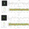 |
Fig. A.1. Method used to extract the 1D H I spectra is presented in the figures above. (a) presents a galaxy that is unresolved by the WRST beam, and (b) a galaxy that is resolved by the beam. A colour cut-out of the galaxy with the extraction aperture overlaid in green is shown in the top left panel. Bottom left panel: location of the 25 reference spectra relative to the target spectrum. Middle top panel: target spectrum, and the middle bottom panel shows the 25 reference spectra. In both middle panels, the vertical dashed green line indicates the redshift of the target galaxy; the orange band represents the gap between the two frequency bands. (a) Source unresolved by the WRST beam. (b) Source resolved by the WRST beam. |
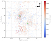 |
Fig. A.2. Bubble plot showing the results of the DS test for the Coma cluster. The δ values are a result of using the 25 nearest neighbours. The red and blue colours indicate the recessional velocity (cz) of each galaxy. The green markers represent the three cD galaxies in Coma (+–NGC 4874, ⋎–NGC 4889 and ×–NGC 4839). The background grey contours represent the X-ray emission measured by ROSAT in 0.4−2.4 keV. |
Number of redshifts obtained from the different literature sources discussed in Sect. 2.1.1.
Appendix B: Stacked spectra
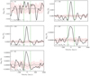 |
Fig. B.1. Stacked spectra from which the full catalogue data points in Fig. 7 are measured. The stacked spectra (the black line) have been smoothed to a velocity resolution of 80 km s−1. The orange band represents the 1σ distribution from 25 stacked reference spectra. The vertical dashed green lines indicate the range over which the spectra are integrated to determine the average integrated flux density for each sample. Each panel represents a different stellar mass bin. The number of spectra in each bin are given in the top left corner of each panel. |
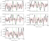 |
Fig. B.3. Coma non-detections stacked in annuli with increasing radius from the cluster centre. The stacked spectra (the black line) have been smoothed to a velocity resolution of 80 km s−1. The orange band represents the 1σ distribution from 25 stacked reference spectra. The vertical dashed green lines indicate the range over which the spectra are integrated to determine the average integrated flux density for each sample. Each panel represents a different stellar mass bin. The number of spectra in each bin are given in the top left corner of each panel. These spectra are used to determine the average DEFH I (DEFH I = log MH I,exp − log MH I,obs) in Fig. 8. |
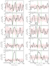 |
Fig. B.6. Stacked spectra for each of the substructures S1–S10. The stacked spectra (the black line) have been smoothed to a velocity resolution of 80 km s−1. The orange band represents the 1σ distribution from 25 stacked reference spectra. The vertical dashed green lines indicate the range over which the spectra are integrated to determine the average integrated flux density for each sample. |
Appendix C: Coma catalogue
Catalogue of Coma galaxies within the Westerbork Coma Survey.
Appendix D: Coma atlas
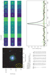 |
Fig. D.1. Atlas page for one galaxy in the WCS. Top left panel: colour image of the galaxy from the DECaLS survey. Overlaid in green on the optical image is an aperture defined by the radius at the B-band 25th mag arcsec−2 isophote; the yellow hatched ellipse indicates the size of the WRST beam. Below the optical image is a table containing the magnitude, reff, axis ratio, position angle, and sersic index of the galaxy in each of the 11 bands. To the right of the optical image are the cut-outs of the galaxy in the 11 photometric bands. Shown below the cut-outs are the best-fit GALFITM model and the residual image for each band. The extracted spectrum for the target galaxy is plotted in black in the bottom right panel, with its optical redshift indicated by the dashed green line. The 25 reference spectra are also shown in this panel in the rainbow colours. Atlas pages for the other Coma galaxies can be found at https://drive.google.com/drive/folders/1sKdnUGgCSi6u-Wf11CwRALW4UFYCvgA4? |
All Tables
Number of redshifts obtained from the different literature sources discussed in Sect. 2.1.1.
All Figures
|
Fig. 1. Colour–magnitude diagram for the Coma cluster. The blue points represent the galaxies in the catalogue of literature redshifts. The black dots represent all galaxies targeted with Hydra, but whose redshifts place them in the foreground or background. The orange open squares represent the galaxies targeted with Hydra with redshifts that place them inside the cluster. Galaxies with r > 17.7 mag and g − r < 0.6 were prioritised as indicated by the dashed red lines. |
| In the text | |
|
Fig. 2. WIYN/Hydra targets, and observed sources. The 5 fields (3 of the fields had a second configuration) targeted with WIYN are indicated by the large circles. The square and diamond data points represent the galaxies we targeted with Hydra. The galaxies with redshifts in the Coma volume are represented by the magenta square data points and the foreground and background galaxies are represented by the blue diamond markers. The green markers represent the three cD galaxies in Coma (+–NGC 4874, ⋎–NGC 4889 and ×–NGC 4839). The 0.4−2.4 keV ROSAT X-ray contours are given by the grey contours (outer contours correspond to 3 × 10⁻⁵ cts s−1, and inner-most contours to 1 × 10⁻³ cts s−1). Other confirmed members of the Coma cluster are represented by the small grey circles. The WCS footprint is indicated by the orange outline. |
| In the text | |
|
Fig. 3. Three examples of the cross-correlation results of Hydra spectra. The dashed lines and grey regions indicate the central wavelength and associated error of the labelled line. The red regions indicate those masked out during the cross-correlation process because of strong sky lines. (a) Good spectrum. (b) Low signal-to-noise. (c) Poor sky subtraction. |
| In the text | |
|
Fig. 4. Distribution of all redshifts (literature and new) within WCS footprint. The red represents the galaxies whose redshifts were obtained using Hydra/WIYN. |
| In the text | |
|
Fig. 5. Galaxy modelled with a single Sersic profile by GALFITM. The input data are shown in the top row, the model in the second row, and the residuals in the bottom row. The colour scale is set in every column such that each row has the same intensity. |
| In the text | |
|
Fig. 6. Stellar mass and star formation distribution of Coma galaxies in the WCS footprint. Left: stellar mass distribution of Coma galaxies within the WCS footprint. Right: star formation rate as a function of stellar mass for the Coma galaxies. The 2σ upper limit on the star formation is shown for galaxies for which there is no detection in the W3 band; these are represented by the light grey points. The step function in the upper limits arises owing to a non-detection in W3 for low-mass galaxies and a non-detection after continuum subtraction in W3 for high-mass galaxies. Also shown for reference are fits to the star formation main sequence by Cluver et al. (2020), Popesso et al. (2019) and Saintonge et al. (2016). The black dashed line indicates the quench threshold (Cluver et al. 2020) below which galaxies are not considered to be actively star forming. |
| In the text | |
|
Fig. 7. Stellar mass (M⋆) to H I gas fraction (fH I) scaling relation for the Coma cluster. The individual 3σ upper limits for the Coma H I non-detections are represented by the grey down-pointing triangles, while the distribution of the individual H I detections is shown by the blue density plot. The pink diamond and orange down-pointing triangle symbols represent the stacking of all Coma galaxies and only non-detections, respectively. The pink diamonds show measurements from a detected stacked spectrum, and the orange triangles indicate the 3σ upper limit in the case of a non-detection in the stacked spectrum. The round light green symbols and green line represent the stacking of field galaxies by Healy et al. (2019) and Fabello et al. (2011), respectively; the dashed green line is an extrapolation of the Fabello et al. (2011) results. The individual fH I measurements (pink stars) for galaxies in the Ursa Major cluster are also shown for reference (Verheijen & Sancisi 2001). |
| In the text | |
|
Fig. 8. H I deficiency of the Coma galaxies as a function of projected radius from the cluster centre. The individual H I deficiency measurements for the Coma galaxies are represented by the green shaded distribution for the H I detections and grey triangles for the lower limits on the H I non-detections. The average H I deficiencies for late-type Coma galaxies from Gavazzi et al. (2006) are shown in orange. The black, blue, and red triangles represent the lower limits from stacking the non-detections in annuli in three samples: all non-detections, log M⋆ < 9.5, and log M⋆ > 9.5, respectively. The horizontal dashed purple lines set the limit on DEFH I values that indicate a galaxy is H I-normal. |
| In the text | |
|
Fig. 9. Phase-space diagram for Coma. The black dashed lines represent the escape velocity for Coma, calculated using a concentration index (c) of 5, M200 = 5.1 × 10¹⁴ M⊙ and r200 = 1.8 Mpc (Gavazzi et al. 2009). Galaxies inside the escape velocity ‘trumpet’ are considered to be within the cluster, while galaxies on the outside edge of the trumpet are considered to be falling into the cluster. The light grey shaded cone represents the virialised zone (Oman et al. 2013). The g − r colour of each galaxy is given by the colour scale in colourbar. |
| In the text | |
|
Fig. 10. Stacked spectra for all (top row), blue (middle row), and red (bottom row) H I non-detections in different regions of the cluster. The average stacked spectrum in each panel is indicated by the solid black, blue, and red lines. The average stacked reference spectrum is represented by the solid grey line. The green band indicates the velocity range cz ± 200 km s−1 over which H I emission is expected to be seen. Only the sample of galaxies outside the r200 (right-most column) of the cluster appear to contain detectable H I. |
| In the text | |
|
Fig. 11. Substructure in the WCS footprint. The 15 identified groups are shown in different colours. The background grey contours represent the X-ray emission measured by ROSAT in 0.4−2.4 keV. The dashed grey lines indicate the direction to nearby clusters connected to Coma. The groups identified by Adami et al. (2005) are labelled and denoted by black crosses. |
| In the text | |
|
Fig. 12. Fifteen identified groups within the WCS footprint. The contours (taken from Adami et al. 2005, Fig. 4) represent the X-ray excess found by Neumann et al. (2003). |
| In the text | |
|
Fig. 13. Stacked spectra for galaxies in groups (top row), and galaxies not in groups (bottom row) separated into different annuli from the cluster centre. The average stacked spectrum in each panel is indicated by a solid black line. The average stacked reference spectrum is represented by a solid grey line, with the variance of 25 stacked reference spectra surrounding the average reference spectrum in orange. The green band is the velocity range cz ± 200 km s−1 over which the H I emission is expected to be seen. |
| In the text | |
|
Fig. 14. Stacked spectra for galaxies in groups (top row), and galaxies not in groups (bottom row) separated into different regions in the cluster. The average stacked spectrum in each panel is indicated by a solid black line. The average stacked reference spectrum is represented by a solid grey line, with the variance of 25 stacked reference spectra surrounding the average reference spectrum in orange. The green band is the velocity range cz ± 200 km s−1 over which the H I emission is expected to be seen. |
| In the text | |
|
Fig. A.1. Method used to extract the 1D H I spectra is presented in the figures above. (a) presents a galaxy that is unresolved by the WRST beam, and (b) a galaxy that is resolved by the beam. A colour cut-out of the galaxy with the extraction aperture overlaid in green is shown in the top left panel. Bottom left panel: location of the 25 reference spectra relative to the target spectrum. Middle top panel: target spectrum, and the middle bottom panel shows the 25 reference spectra. In both middle panels, the vertical dashed green line indicates the redshift of the target galaxy; the orange band represents the gap between the two frequency bands. (a) Source unresolved by the WRST beam. (b) Source resolved by the WRST beam. |
| In the text | |
|
Fig. A.2. Bubble plot showing the results of the DS test for the Coma cluster. The δ values are a result of using the 25 nearest neighbours. The red and blue colours indicate the recessional velocity (cz) of each galaxy. The green markers represent the three cD galaxies in Coma (+–NGC 4874, ⋎–NGC 4889 and ×–NGC 4839). The background grey contours represent the X-ray emission measured by ROSAT in 0.4−2.4 keV. |
| In the text | |
|
Fig. B.1. Stacked spectra from which the full catalogue data points in Fig. 7 are measured. The stacked spectra (the black line) have been smoothed to a velocity resolution of 80 km s−1. The orange band represents the 1σ distribution from 25 stacked reference spectra. The vertical dashed green lines indicate the range over which the spectra are integrated to determine the average integrated flux density for each sample. Each panel represents a different stellar mass bin. The number of spectra in each bin are given in the top left corner of each panel. |
| In the text | |
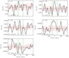 |
Fig. B.2. Same as Fig. B.1, for the sample of H I non-detections. |
| In the text | |
|
Fig. B.3. Coma non-detections stacked in annuli with increasing radius from the cluster centre. The stacked spectra (the black line) have been smoothed to a velocity resolution of 80 km s−1. The orange band represents the 1σ distribution from 25 stacked reference spectra. The vertical dashed green lines indicate the range over which the spectra are integrated to determine the average integrated flux density for each sample. Each panel represents a different stellar mass bin. The number of spectra in each bin are given in the top left corner of each panel. These spectra are used to determine the average DEFH I (DEFH I = log MH I,exp − log MH I,obs) in Fig. 8. |
| In the text | |
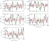 |
Fig. B.4. Same as Fig. B.3 for the sample of galaxies with log M⋆ < 9.5. |
| In the text | |
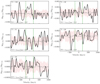 |
Fig. B.5. Same as Fig. B.3 for the sample of galaxies with log M⋆ > 9.5. |
| In the text | |
|
Fig. B.6. Stacked spectra for each of the substructures S1–S10. The stacked spectra (the black line) have been smoothed to a velocity resolution of 80 km s−1. The orange band represents the 1σ distribution from 25 stacked reference spectra. The vertical dashed green lines indicate the range over which the spectra are integrated to determine the average integrated flux density for each sample. |
| In the text | |
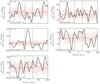 |
Fig. B.7. Same as Fig. B.6, but for substructures S11–S15. |
| In the text | |
|
Fig. D.1. Atlas page for one galaxy in the WCS. Top left panel: colour image of the galaxy from the DECaLS survey. Overlaid in green on the optical image is an aperture defined by the radius at the B-band 25th mag arcsec−2 isophote; the yellow hatched ellipse indicates the size of the WRST beam. Below the optical image is a table containing the magnitude, reff, axis ratio, position angle, and sersic index of the galaxy in each of the 11 bands. To the right of the optical image are the cut-outs of the galaxy in the 11 photometric bands. Shown below the cut-outs are the best-fit GALFITM model and the residual image for each band. The extracted spectrum for the target galaxy is plotted in black in the bottom right panel, with its optical redshift indicated by the dashed green line. The 25 reference spectra are also shown in this panel in the rainbow colours. Atlas pages for the other Coma galaxies can be found at https://drive.google.com/drive/folders/1sKdnUGgCSi6u-Wf11CwRALW4UFYCvgA4? |
| In the text | |
Current usage metrics show cumulative count of Article Views (full-text article views including HTML views, PDF and ePub downloads, according to the available data) and Abstracts Views on Vision4Press platform.
Data correspond to usage on the plateform after 2015. The current usage metrics is available 48-96 hours after online publication and is updated daily on week days.
Initial download of the metrics may take a while.