| Issue |
A&A
Volume 649, May 2021
|
|
|---|---|---|
| Article Number | A19 | |
| Number of page(s) | 25 | |
| Section | Interstellar and circumstellar matter | |
| DOI | https://doi.org/10.1051/0004-6361/202039733 | |
| Published online | 28 April 2021 | |
Measuring the ratio of the gas and dust emission radii of protoplanetary disks in the Lupus star-forming region
1
European Southern Observatory,
Karl-Schwarzschild-Strasse 2,
85748
Garching bei München,
Germany
e-mail: This email address is being protected from spambots. You need JavaScript enabled to view it.
2
Universitäts-Sternwarte, Ludwig-Maximilians-Universität München,
Scheinerstrasse 1,
81679
München,
Germany
3
Excellence Cluster Origins,
Boltzmannstrasse 2,
85748
Garching bei München,
Germany
4
INAF/Osservatorio Astrofisico di Arcetri,
Largo E. Fermi 5,
50125
Firenze,
Italy
5
School of Cosmic Physics, Dublin Institute for Advanced Studies,
31 Fitzwilliams Place,
Dublin 2,
Ireland
6
Max Planck Institute for Astronomy,
Königstuhl 17,
69117
Heidelberg,
Germany
7
Joint ALMA Observatory,
Av. Alonso de Córdova 3107,
Vitacura,
Santiago,
Chile
8
Núcleo Milenio Formación Planetaria - NPF, Universidad de Valparaíso,
Av. Gran Bretaña 1111,
Valparaíso,
Chile
9
European Southern Observatory,
3107, Alonso de Córdova,
Santiago de Chile,
Chile
10
Department of Astronomy, Cornell University,
Ithaca,
NY
14853,
USA
11
Atacama Large Millimeter/Submillimeter Array, Joint ALMA Observatory,
Alonso de Córdova 3107,
Vitacura
763-0355,
Santiago,
Chile
12
CENTRA, Faculdade de Ciências, Universidade de Lisboa,
Ed. C8, Campo Grande,
1749-016
Lisboa,
Portugal
13
Lunar and Planetary Laboratory, The University of Arizona,
Tucson,
AZ
85721,
USA
14
Earths in Other Solar Systems Team, NASA Nexus for Exoplanet System Science,
USA
15
Institute for Astronomy, University of Hawaii,
Honolulu,
HI
96822,
USA
Received:
21
October
2020
Accepted:
18
January
2021
Abstract
We performed a comprehensive demographic study of the CO extent relative to dust of the disk population in the Lupus clouds in order to find indications of dust evolution and possible correlations with other disk properties. We increased the number of disks of the region with measured RCO and Rdust from observations with the Atacama Large Millimeter/submillimeter Array to 42, based on the gas emission in the 12CO J = 2−1 rotational transition and large dust grains emission at ~0.89 mm. The CO integrated emission map is modeled with an elliptical Gaussian or Nuker function, depending on the quantified residuals; the continuum is fit to a Nuker profile from interferometric modeling. The CO and dust sizes, namely the radii enclosing a certain fraction of the respective total flux (e.g., R68%), are inferred from the modeling. The CO emission is more extended than the dust continuum, with a R68%CO/R68%dust median value of 2.5, for the entire population and for a subsample with high completeness. Six disks, around 15% of the Lupus disk population, have a size ratio above 4. Based on thermo-chemical modeling, this value can only be explained if the disk has undergone grain growth and radial drift. These disks do not have unusual properties, and their properties spread across the population’s ranges of stellar mass (M⋆), disk mass (Mdisk), CO and dust sizes (RCO, Rdust), and mass accretion of the entire population. We searched for correlations between the size ratio and M⋆, Mdisk, RCO, and Rdust: only a weak monotonic anticorrelation with the Rdust is found, which would imply that dust evolution is more prominent in more compact dusty disks. The lack of strong correlations is remarkable: the sample covers a wide range of stellar and disk properties, and the majority of the disks have very similar size ratios. This result suggests that the bulk of the disk population may behave alike and be in a similar evolutionary stage, independent of the stellar and disk properties. These results should be further investigated, since the optical depth difference between CO and dust continuum might play a major role in the observed size ratios of the population. Lastly, we find a monotonic correlation between the CO flux and the CO size. The results for the majority of the disks are consistent with optically thick emission and an average CO temperature of around 30 K; however, the exact value of the temperature is difficult to constrain.
Key words: stars: pre-main sequence / protoplanetary disks / planets and satellites: formation / submillimeter: general
© ESO 2021
1 Introduction
Planets form around stars during their pre-main-sequence phase, when still surrounded by a circumstellar disk of gas and dust. Setting observational constraints on the gas and dust properties of these disks is crucial in order to understand the ongoing physical processes in the disk. These processes shape the planet formation mechanisms, and ultimately tell us about the disk’s ability to form planets (see, e.g., Mordasini et al. 2012).
The advent of the Atacama Large Millimeter/submillimeter Array (ALMA) allowed for a characterization of the dust properties in large populations of disks (e.g., Tazzari et al. 2017; Andrews et al. 2018b; Hendler et al. 2020), based on surveys targeting nearby star-forming regions (Ansdell et al. 2016, 2017; Barenfeld et al. 2016; Pascucci et al. 2016; Cox et al. 2017; Cieza et al. 2018; Cazzoletti et al. 2019; Williams et al. 2019). However, demographic studies of the gas disk properties in these regions are scarcer (e.g., Long et al. 2017; Ansdell et al. 2018; Najita & Bergin 2018; Boyden & Eisner 2020, due to the fewer detections, the difficulty of finding reliable gas tracers (e.g., Miotello et al. 2016, 2017), and, frequently, cloud contamination.
A key diagnostic of the evolutionary stage of a disk is its size. Dust and gas evolve differently, thus we can learn about the physical processes undergone in the disk by studying the relative extent between gas and dust (e.g., Sellek et al. 2020a,b). Initially, the dust grains have sizes below 1 μm and are kinematically coupled to the gas (e.g., Fouchet et al. 2007; Birnstiel et al. 2010). The pressure gradient of a disk, which generally points outward, exerts an additional force that causes gas to orbit in a slightly sub-Keplerian speed. Dust grains grow by coagulation and when large enough – of the order of millimeter (mm) sizes – orbiting grains are no longer supported by the outward pressure force. A frictional force is induced on the large grains, and, by angular momentum conservation, a drift inwards that results in piled-up large grains in a compact configuration (e.g., Weidenschilling 1977; Pinilla et al. 2012; Canovas et al. 2016). On the other hand, gas in viscous disks spreads out to conserve angular momentum and enable close-in gas to accrete ontothe star (e.g., Lynden-Bell & Pringle 1974; Nakamoto & Nakagawa 1994; Hueso & Guillot 2005). In wind-driven accretion models (for a review, see Turner et al. 2014), the gas extent will also be larger than the dust extent: dust still drifts inwards, while the gas extent does not vary significantly. Observations at (sub-)mm wavelengths typically trace the large dust grains (sizes up to cm sizes) decoupled from the gas (Testi et al. 2014; Andrews 2015); hence, disks that have undergone dust evolution will appear more extended in gas than in dust continuum from ALMA observations.
A difference in size between the gas and dust content has been confirmed from observations of individual young stellar objects (YSOs; e.g., Isella et al. 2007; Andrews et al. 2012), and, thanks to ALMA, also from larger samples (e.g., Ansdell et al. 2018; Boyden & Eisner 2020). Besides the effect of dust evolution, the optical depth difference between dust continuum and gas rotational lines may also contribute to the disparity in the observed gas and dust sizes (e.g., Trapman et al. 2019). While dust thermal emission in the outer disk is optically thin or only partially thick (e.g., Huang et al. 2018), the gas emission is, in general, optically thicker (e.g., Guilloteau & Dutrey 1998). A difference in optical depth implies the dust emission is fainter than the gas rotational line, thus the emission of the dust outer disk would fall below the sensitivity limit of the instrument at a smaller radius compared to the gas outer emission.
Consequently, identifying the effect that dominates the size ratio is not easy. Trapman et al. (2019) showed that disks with gas-dust size ratios above 4 can only be explained if grain growth and subsequent radial drift has occurred. Such high size ratios between gas and dust have already been observed (Facchini et al. 2019). The existence of pressure bumps can also limit the study of dust evolution based on the gas-dust size ratio. In the latter scenario, dust grains from the outer disk would only drift inwards down to the bump location. This might result in a larger observed dust size, thus a lower size ratio.
In this work, we expanded on the previous study of the gas and dust content in the protoplanetary disk population of Lupus (Ansdell et al. 2018). The gas extent was measured based on emission of 12CO rotational lines at (sub-)mm wavelengths, while the dust extent was obtained from the continuum emission of large grains. The CO emission from these lines is appropriate for the study of the gas extent due to its abundance. These lines are optically thick at low CO column densities (van Dishoeck & Black 1988), allowing CO to self-shield and avoid photodissociation from UV photons. Extremely low CO temperatures (of ~ 20 K) limits the study of gas based on these lines, since CO may freeze out onto the dust grains’ surface, no longer emitting at these rotational lines.
The integrated CO emission was modeled to empirical functions, this allowed us to increase the number of disks with characterized CO compared to previous studies. In addition, disks surrounding brown dwarfs (BDs) from more recent observations (Sanchis et al. 2020) were added to the studied sample. Dust disk sizes were estimated by fitting empirical models in the visibility plane. This paper is organized as follows: in Sect. 2, we describe the Lupus disk sample and the observations used; the modeling of the CO and dust continuum emission is presented in Sect. 3; the resulting sizes are summarized in Sect. 4; in Sect. 5, we perform the demographic analysis of the CO and dust sizes and discuss what the results entail; finally, in Sect. 6, we summarize the main findings of this study.
2 Sample selection
The objects studied in this work belong to the Lupus clouds (I–IV), a low-mass star-forming region (SFR) that is part of the Scorpius-Centaurus OB association (Comerón 2008). Lupus is one of the closest SFRs, at a median distance of 158.5 pc (from individual Gaia parallaxes of the Lupus members, Gaia Collaboration 2018). The age of the region is approximately 1–3 Myr (Comerón 2008; Alcalá et al. 2017).
The sample includes young stellar objects with confirmed protoplanetary disks, down to the BD regime (we define BDs as systems of spectral type equal to or later than M6, and whose central object mass is < 0.1 M⊙ ). The sources were selected from the catalogs of the clouds (Hughes et al. 1994; Mortier et al. 2011; Merín et al. 2008; Comerón 2008; Dunham et al. 2015; Bustamante et al. 2015; Mužić et al. 2014, 2015), their infrared (IR) excess estimated from Spitzer (‘Cores to Discs’ legacy project, Evans et al. 2009) and 2MASS (Cutri et al. 2003) data. Details on the sample selection for the ALMA surveys are to be found in Ansdell et al. (2016, 2018) for the stellar objects and Sanchis et al. (2020) for the BDs. All objects are confirmed members of the Lupus clouds from radial velocity analysis (Frasca et al. 2017). The stellar properties were taken from Alcalá et al. (2014, 2017) and Mužić et al. (2014), while stellar luminosities (L⋆ ) and masses (M⋆) were recalculated taking into account the distance from the precise Gaia DR2 parallaxes (Gaia Collaboration 2018; Manara et al. 2018; Alcalá et al. 2019). The stellar mass was obtained from the position in the Hertzsprung–Russell (HR) diagram set by the effective temperature and the updated L⋆ . The stellar mass was primarily interpolated from the pre-main-sequence models of Baraffe et al. (2015), which provide accurate estimates of M⋆ for BDs, M dwarfs, and low-mass stars up to 1.4 M⊙ . These models are ideal for our sample, since the great majority of Lupus objects are within this mass range. For the very few objects above 1.4 M⊙ (only three in the entire Lupus sample) the Siess et al. (2000) models were used instead. The stellar mass uncertainty was obtained from a Markov chain Monte Carlo (MCMC) procedure as in Alcalá et al. (2017).
Following these criteria, the selected ALMA dataset is composed of 100 protoplanetary disks around YSOs in the Lupus clouds, nine of which are BDs. However, our analysis concentrates on the 42 disks whose CO and dust radii could be measured.
Observations
The CO radial extent of the disks was measured from archival ALMA observations covering the 12CO J = 2−1 rotational line in Band 6 (at 230.538 GHz). For three sources, the J = 3−2 rotational transition inBand 7 (at 345.796 GHz) was used instead. The dust sizes were obtained based on the modeling of archival observations of dust continuum in ALMA Band 7 (centered at ~ 0.89 mm). The 12CO channel maps were built after subtracting the continuum and cleaning with a Briggs weighting and robustness = +0.5. In Table 1, the details of the line and continuum ALMA observations used in this study are summarized; this includes information concerning the ALMA project IDs, the number of Lupus sources targeted at each ALMA project, angular resolution, and the corresponding references that describe the observations and the instrument configuration.
In order to test our method for determining the CO disk radial extent for a few disks in the dataset described above, we analyzed available ALMA data at higher resolution and better sensitivity. These additional data were part of the DSHARP large program (for a general description of the project, see Andrews et al. 2018a; see also the other DSHARP publications II-X) that also covered the 12CO J = 2–1 rotational transition for all targets. The Lupus disks targeted in DSHARP are Sz 68 (HT Lup), Sz 71 (GW Lup), Sz 82 (IM Lup), Sz 83 (RU Lup), Sz 114, Sz 129, and MY Lup. Lastly, the continuum dataset of the Band 6 Lupus disk survey was used to test the dust size results between this and previous work (Ansdell et al. 2018).
Summary of archival ALMA projects used in this work for the gas and dust modeling.
3 Modeling
The methodology employed to measure the gas and dust sizes of the Lupus disk population is described in this section.
3.1 CO modeling
The CO emission of each disk was primarily modeled by fitting the integrated line map to an elliptical Gaussian function in the image plane. For disks in which a Gaussian model does not conveniently describe the observed CO emission, the so-called Nuker profile model (e.g., Lauer et al. 1995; Tripathi et al. 2017) was used instead. We assessed the quality of the Gaussian fit by comparing its radii results to those from high angular resolution and sensitivity observations, and by quantifying the residuals between the observation and the model. This is explained in detail in Sect. 3.1.2.
This modeling is appropriate for the CO disks characterization due to the low signal-to-noise ratio (S/N) for the bulk of the sample. Theintegrated map was obtained by summing up all the channels showing emission above noise level around the known position of the object; the range of channels were selected based on a visual examination of the channel maps and spectrum. For the elliptical Gaussian modeling, the imfit task from CASA software (McMullin et al. 2007) was used. The task provides the parameter values with uncertainties of the Gaussian fit to the observed emission. The Nuker profile modeling was performed by fitting1 the azimuthally averaged CO emission to this function, centered at the optimal position from the imfit results. The outer edge of the Nuker model was set as the radius in which the azimuthally averaged profile first reaches zero.
3.1.1 Size definition
The size definition used in this work is the radius enclosing a certain fraction of the total modeled flux, for the CO (RCO ) and for the dust (Rdust) components, separately. This definition has recently been used to characterize large samples of disks from ALMA observations (e.g., Tazzari et al. 2017; Andrews et al. 2018b; Hendler et al. 2020), and for the theoretical modeling of disks (e.g., Rosotti et al. 2019; Trapman et al. 2019, 2020). The fractions considered are 68, 90, and 95% for easy comparison with previous works. To estimate the CO radii, we first obtained the deprojected model emission profile, either from the deconvolved major-axis full width at half maximum (FWHM) of the elliptical Gaussian model, or from the optimal values of the parameters in the Nuker fitting. We then produced the cumulative distribution functions (fcumul, following, e.g., Eq. (A.1) in Sanchis et al. 2020). The radius (e.g., R68%) is inferred from the expression fcumul(R68%) = 0.68 ⋅ Ftot, where Ftot is the total integrated line emission of the model. For the elliptical Gaussian models, the R68% can be obtained from the standard deviation (σ) of the respective model with the formula:
 (1)
(1)
The uncertainty of the CO sizes was obtained from the major-axis FWHM error on the Gaussian fits. For the Nuker fitting of CO, the size uncertainties were acquired from a MCMC procedure as follows: 1000 realizations of the free parameters were drawn from a random normal distribution defined by the parameters’ optimal values and their standard deviation, and from this set of values we built 1000 Nuker models and measured their R68% , R90% , and R95% . Their associated standard deviation was taken as the size uncertainty of the Nuker models.
The method to infer CO sizes of the Lupus disk population differs from the approach in Ansdell et al. (2018). In that work, the CO size was estimated from the curve of growth of Keplerian masked moment zero maps. The Keplerian masking assumes a physical model in which gas kinematics are described by Keplerian rotation. Their moment zero map was built from selected emission on each channel that is expected to come from the disk. We avoided thisapproach in order to keep our analysis as general as possible, without any assumptions on the disk physics. Additionally, sizes of fainter sources are difficult to measure using the curve of growth, since there is no clear end of the disk emission there. In Sect. 4.1, we compare our sizes to the results of Ansdell et al. (2018).
Lastly, we note that the sizes of three BD disks (SSTc2d J154518.5-342125, 2MASS J16085953-3856275, and Lup706) were obtained from the emission of a different line (12CO J = 3−2). Differences in the measured radii between this line and the 12CO J = 2−1 line are expected to be negligible, since the two lines are being emitted from essentially the same layer in the disk atmosphere, therefore at almost identical temperatures.
3.1.2 CO size uncertainties, from comparison to the DSHARP survey
The purpose of this section is to assess the systematic errors of the CO modeling used and to find a reliable criterion to determine in which cases the CO emission can be modeled to an elliptical Gaussian or to a Nuker profile model instead. To accomplish these goals, we compared the radii of six disks from our sample to the radii from additional 12CO (J = 2−1) observations of the same objects at higher angular resolution and sensitivity (DSHARP project, details in Andrews et al. 2018a).
In order to perform this comparison, a reliable measurement of the CO disk sizes from the DSHARP data is required, and these are treated as the fiducial sizes of these disks. This was accomplished via interferometric modeling of the 12CO line visibilities: channels with line emission were continuum-subtracted and then spectrally integrated, and the resulting visibilities were then modeled by a Nuker profile model. A comprehensive description of this modeling can be found in Appendix A. In Appendix B, we summarize the CO sizes using different methodologies for the two datasets (resulting sizes tabulated in Table B.1).
We compared the R68% from the elliptical Gaussian modeling of the Lupus disk survey with the fiducial sizes from the interferometric modeling of the DSHARP data (Fig. B.1). For all the disks except one, the elliptical Gaussian modeling yields smaller sizes than the fiducial values. One disk (MY Lup) has nearly identical size results between the two datasets, a second disk (Sz 114) has a size deviation below 20%, two other objects (Sz 71 and Sz 129) have ~30% difference between the inferred sizes, and the last two sources (Sz 82 and Sz 83) have a discrepancy above 40%. When inspecting the R90% radii, the discrepancies are slightly increased, with only three disks with a size deviation below 30%, and discrepancies beyond 40% for the remaining disks.
Several factors might contribute to the difference in the measured sizes. Firstly, the difference in sensitivity between observationscan affect the detection of emission in the outermost regions of the disk. In addition, the different angular resolution may also have an impact: in general, the better resolved the disk, the better the size measurement. Another possible cause is the act of modeling the Lupus disk population in the image plane, while the fiducial sizes are obtained from modeling in the uv-plane. Lastly, the size difference could be due to the elliptical Gaussian model not being able to reproduce the true CO emission. To understand the impact of these effects, we studied them separately.
The sensitivity difference was tested using the exact same method to model the two datasets, that is, fitting elliptical Gaussian models to the disk survey and to the DSHARP sets. The results are included in Table B.1. The measured sizes between the two datasets are very similar, with only ~ 5% difference. Therefore, sensitivity has a minor effect on the inferred CO sizes of the Lupus disk dataset. The effect of the angular resolution can also be inspected from this comparison. The angular resolution has a stronger effect on smaller disks (i.e., of the order of the beam size). The two smallest disks (Sz 129 and MY Lup) show a slightly larger size difference of ~ 15% compared tothe aforementioned difference of the sample. Although the sample considered is very limited, our results show that a resolution effect might be relevant, especially in disks of size of the order of the beam size.
The effect of measuring the CO radial extent from modeling the emission in the image or in the uv-plane was investigated by modeling the same dataset with the same empirical function (i.e., elliptical Gaussian) in both planes. For each disk of the DSHARP dataset, we reconstructed the moment zero maps from the line visibilities; the imfit task was then used for the Gaussian modeling in the image plane. The interferometric modeling was analogous to the methodology described in Appendix A, but using a Gaussian function instead of the Nuker function. The size results are included in Table B.1. The difference in size is negligible for every disk, 2% on average, therefore modeling the emission in the image plane has a negligible effect on the inferred size.
Lastly, we tested the accuracy of the Gaussian modeling with respect to the Nuker profile modeling. We compared the interferometric modeling results when fitting the DSHARP data to a Gaussian or a Nuker profile. The results (Table B.1) show a size difference of ~20% on average. Two disks (MY Lup and Sz 129) have size differences below 5%; one disk (Sz 114) has a difference of ≲ 15%; another disk (GW Lup) has a difference of around 30%; and the remaining two disks have differences beyond 40%.
Hence, the Gaussian modeling not reproducing the observed emission of certain objects is the most limiting effect on the CO size determination. It yields accurate CO sizes in several disks, but in other disks (typically those with extended emission) the inferred sizes can differ significantly with respect to the true CO extent. For those disks, the Nuker model is able to accurately describe theextended emission of the disk. In order to determine which CO disks can be described by an elliptical Gaussian model, we developed a criterion that evaluates the quality of the model, based on the amount of residuals (difference between observed and modeled emission). This criterion is described in detail in Appendix C.
Based on this criterion, the CO emission was fit to an elliptical Gaussian for those disk models with negligible residuals (i.e., when the quantified residuals are outside the μ ± σ range of the entire population), otherwise the emission was fit to a Nuker function.
In summary, our modeling in the image plane typically allowed us to measure the CO sizes for the Lupus disk sample with an uncertainty ≲30%, based on the comparison with available observations at higher resolution and sensitivity. Due to its simplicity and its ability to reproduce the observed CO emission, we used the elliptical Gaussian modeling for the cases in which the measured RCO is reliable. For CO disks with Gaussian model residuals outside the valid range, the Nuker modeling in the image plane was used instead.
3.2 Dust modeling
The dust disks were modeled in the uv-plane to an empirical function called the Nuker profile. We refer the reader to Sanchis et al. (2020) for a detailed description of the interferometric modeling, in which the Galario package (Tazzari et al. 2018) was used in combination with a MCMC procedure to model the continuum emission of the BD disks and sources from the Lupus disk completion survey. In the present work, we took the Rdust results of Sanchis et al. (2020) for the ten disks with detected 12CO and modeled the remaining disks of the Lupus population using identical methodology. The dust sizes considered are the radii enclosing 68, 90, and 95% of the total disk emission, analogous to the size definition of the CO disk.
Performing the modeling in the uv-plane may reduce possible uncertainties associated with the image reconstruction process. Nevertheless, we tested the resulting dust sizes when modeling to a Nuker function in the image plane for a number of resolved disks. The results are in very good agreement with the dust sizes obtained from fitting the visibilities (deviation of ~ 5%). Thus, modeling the continuum emission in the image or in the uv-plane does not have a significant impact on the size results. Only for very compact sources may the sizes obtained from the image plane modeling be affected by the beam.
4 Disk size results
4.1 CO size results
The CO-disk size results of the Lupus disk population are presented in this section. We excluded the results from disks with a model peak less than three times the rms of the observed moment zero map, those with maps partially covered by clouds, and disks that belong to binary systems with angular separation below 2′′ . The resulting CO disk sizes (R68%) are summarized in Table 2. The uncertainties in the table are associated with the fitting method employed. Nevertheless, we warn that the inferred CO sizes may have a discrepancy of 0 ~ 30% with respect to the true CO extent, based on our tests described in Sect. 3.1.2.
By definition of the Gaussian function, there is a constant relation between the R68% and the two other radii (R90%, R95%):
 (2)
(2)
and
 (3)
(3)
The above relations can be used to obtain the R90% and R95% radii for the CO Gaussian models. For the disks modeled with the Nuker function, we provide the optimal parameters of the fit in Appendix D.
Out of 51 disks detected in CO, three are partially covered by clouds (J15450634-3417378, J15450887-3417333, J16011549-4152351), another three yield models of which the S/N is too low (Sz 98, J16085324-3914401, J16095628-3859518), and three belong to close binary systems (Sz 68, Sz 74, Sz 123A). Therefore, our methodology allowed us to model the emission and size of 42 disks. Three of these CO sizes are provided as upper limits (with the tabulated value being the 95% confidence level) since the deconvolved FWHM of their elliptical Gaussian models exhibits a point-like nature. Additionally, two of these objects with CO size upper limits are disks around BDs. Table 2 includes a column stating the CO model used to infer the CO sizes (the elliptical Gaussian model is referred to as ‘G’ and the Nuker model as ‘N’). In Appendix E, we include the observed, modeled, and residual CO maps, together with the line spectrum and the modeled intensity profile of every disk with measured CO size. Cloud absorption is seen on the line spectrum for a considerable number of sources. This reduces the integrated flux of the line. However, it should not have a significant incidence in the measured CO radii (Ansdell et al. 2018).
Lastly, molecular outflows from 12CO observationshave been reported in at least three of the tabulated sources based on the dynamical analysis of the CO emission (EX Lup, V1192 Sco, Sz 83; Hales et al. 2018; Santamaría-Miranda et al. 2020; Huang et al. 2020). The outflows of the first two objects are within the reported CO sizes in Table 2. Our sizes were obtained by modeling the total integrated emission detected, thus a fraction of the modeled emission does not belong to the disk but to the molecular outflows. Therefore, we consider the inferred CO sizes of EX Lup and V1192 Sco as upper limits. On the other hand, Sz 83 shows a very intricate structure with spirals, jets, and clumps of emission (Herczeg et al. 2005; Ansdell et al. 2018; Andrews et al. 2018a; Huang et al. 2020). We discuss this disk in greater detail in Appendix F, together with other singular systems of the sample. Our CO size reported in Table 2 is larger than the Keplerian disk size and the surrounding non-Keplerian emission, and it might contain a fraction of the emission from the spiral arms (Huang et al. 2020). For consistency, we used the CO size measured by our methodology, although we warn that the true value of the CO disk size might differ.
In the left panel of Fig. 1, we compare our results to the 22  sizes from Ansdell et al. (2018), derived using the curve-of-growth method on Keplerian masked CO maps. The
  was used for this comparison, since it is the only reported size in Ansdell et al. (2018). Due to the different methodology between the two studies, the comparison between the two studies using
  and
and  might differfrom Fig. 1 due to the difference in methodology. However, the
  , which is the radius used in the discussion section of this paper (Sect. 5), will typically show lower discrepancies, since it is less affected by the low sensitivity on the outermost regions of the disks.
The CO sizes from the two methods are in good agreement for the majority of disks, only one object (Sz 82) has a difference in radius above 30%. This object is the largest CO disk of the Lupus population, and this size divergence is likely due to the contrasting approach of the methods. The radius from Ansdell et al. (2018) was inferred from a moment zero map built from selected emission at each channel expected by Keplerian rotation of the gas, while in this work there is no assumption on the velocity structure of the observed CO. The Sz 82 disk has an extremely large tail of emission (as seen in the integrated maps of the object, Fig. E.1) that was not captured in the modeling from Ansdell et al. (2018), and it explains the large size difference between the two studies. This extended emission has already been observed (Cleeves et al. 2016; Pinte et al. 2018). In Appendix F, we discuss in detail the Sz 82 disk, together with other singular objects of the Lupus population.
Results of CO and dust sizes for the Lupus disk sample.
4.2 Dust size results
The resulting radii from the dust modeling are summarized in Table 2, together with uncertainties. For disks in which the dust emission is not appropriately modeled, we provide upper limits of the sizes, estimated as the 95th percentile of the corresponding size.
The protoplanetary disk sample of the Lupus region has been modeled in various studies (e.g., Tazzari et al. 2017; Andrews et al. 2018b; Hendler et al. 2020) based on the same ALMA Band 7 surveys. Our dust disk results can be directly compared to those from the literature (see right panel in Fig. 1). In general, the  results are in very good agreement with the results of Andrews et al. (2018b) and Hendler et al. (2020), the studies that characterized the dust sizes for a larger sample of Lupus disks. Only five disks have differences above 20% with respectto the
  from Andrews et al. (2018b). Three of those disks (Sz 66, Sz 72, Sz 131) are marginally resolved in continuum, and sizes among the three studies vary between 0.08 and 0.11′′. The remaining two are SSTc2d J160703.9-391112, which has large uncertainties in the three studies, nevertheless, our results are compatible within error bars, and Sz 73, for which
  from our modeling is in good agreement with Hendler et al. (2020). Lastly, when comparing our
  with the outer radii results for the subsample of disks studied in Tazzari et al. (2017), our results are in very good agreement, with only four objects presenting differences greater than 20%. In this case, the differences in radii might arise due to the modeling approach. Instead of an empirical function, Tazzari et al. (2017) fit the emission to a physical model, which can result in a different model emission profile. Besides this, the
  used for the comparison is expected to have larger uncertainties than
  , since it is more affected by the low signal of the outermost disk.
The dust sizes presented in this work are based on (sub-)mm continuum emission, which typically probes the population of large dust grains at the disk’s mid-plane. These sizes are appropriate to constrain dust evolution of the disks. Observations in other wavelengths can also be used to infer the size of the disks. For instance, scattered-light imaging at near infrared (NIR) wavelengths probes micron-sized grains – dynamically more coupled to gas – in the upper atmospheric layers of the disk. Five disks in our sample were recently observed with VLT/SPHERE (Avenhaus et al. 2018; Garufi et al. 2020). We can compare the extent of the disks in NIR observations to our size results by taking the outermost radius at which the signal in NIR is detected and our R95%. The sizes from NIR observations are on average ~40% larger than our  , expected since the smaller grains are more dynamically bound to gas. The NIR sizes are, on the other hand, ~ 50% smaller than our
  . This comparison is limited due to the very different nature of the observations, the differing definition of the size, and the narrow sample of disks imaged in NIR.
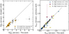 |
Fig. 1 Left panel: comparison between |

4.3 Gas/dust size ratio results
In this and following sections we focus our analysis and discussion on the radii enclosing 68% of the CO and dust fluxes (R68%) instead of R90% or R95%. This is due to the moderate sensitivity of the observations, which could affect the detection of weak emission, typically in the outermost regions of the disk. This might have an impact in the outer slope of model emission when fitting to a Nuker profile. The R68% radius is less affected than R90% and R95% by the outer slope of the model. Since our dataset was assembled by combining various surveys with different resolutions and sensitivity levels, we favored the use of the R68% to reduce this possible effect. We also warn the reader that in the following analysis and figures, the size uncertainties used are the ones derived from the respective method employed. However, CO sizes based on this dataset might have a discrepancy with respect to the true CO size between 0 and ~ 30%, as explained inSect. 3.1.2.
In Fig. 2, we show the histograms and cumulative distributions of the radii (RCO and Rdust) of all the Lupus disks with measured CO and dust sizes. The radii were obtained for each disk following the methodology described in Sect. 3. A difference between the CO disk and the dust disk sizes becomes apparent from the figure. The Anderson–Darling test2 yields a <0.001% probability that the two radii histograms are drawn by the same parent distribution. There is a selection effect toward larger CO sizes, since it is more difficult to detect and measure CO sizes as small as the dust sizes. Nevertheless, the fraction of disks with measured Rdust and unknown RCO is small (around 20% of disks with known Rdust), thus this effect would not change the observed size difference. This disparity in sizes was already reported in Ansdell et al. (2018) for a smaller sample of the Lupus disk population, and in other SFRs, such as Taurus (Najita & Bergin 2018) and Orion (Boyden & Eisner 2020).
In order to investigate the relative size of CO with respect to the dust continuum, we inspected the ratio between RCO against Rdust. In Fig. 3, the radii enclosing 68% of the respective total fluxes are shown, with dashed lines representing the 1, 2, 3, and 4 ratios between CO and dust radii. The median of the  /
/  ratio is 2.5, excluding disks with an upper-limit value in CO and/or dust size. The dispersion of this sample (considered as the standard deviation of the size ratio sample) is relatively high(1.5) and is raised by the few disks with very high size ratios. When using the R90% CO and dust radii, the median and dispersion of the size ratio are slightly larger, with values of 2.7 and 1.5, respectively. In Appendix F, we describe disks from singular objects in more detail; namely, disks with very high size ratios (F.1–F.6), the brightest object of the sample (Sz 82, F.7), and the results of disks around BDs and very low-mass stars (F.8). We also note that a few disks with measured sizes are orbiting a component of a binary or multiple system. We only considered systems with a relatively large angular separation between components (>2″). The impact of binarity and effects such as tidal truncation cannot be constrained based on our limited sample of disks that are part of a multiple system.
The measured size ratios might be even larger on compact objects. Trapman et al. (2019) showed that the measured size ratio is lower than the true value on disks with sizes similar to the beam size. On the other hand, the demographics analysis is affected by a lower completeness of fainter and non-detected CO disks. These disks would likely have small CO-dust size ratios. There are indeed a number of disks with measured Rdust but without RCO. However, these disks spread over the entire M⋆ range, and therefore, they should not have a significant incidence on our demographic analysis.
In the Lupus sample, most of the disks around more massive stars are detected in both CO and dust and the sizes could be characterized. The completeness level at the low M⋆ range of the sample is lower, since disks around less massive objects are generally fainter in continuum and line emission. Therefore, we focused on the solar mass range subsample in order to reduce the possible biases due to a lower completeness. In the stellar mass range between 0.7 and 1.1 M⊙, the total number of protoplanetary disks in the Lupus sample considered (Sect. 2) is ten. All of them were detected in 12CO and dust continuum. One source (Sz 68) was excluded from the analysis since it is a multiple system with an angular separation below 2″. Another object (Sz 77) has an upper limit on the Rdust. The remaining eight disks have measured radii in 12CO and dust continuum. The size ratio median in this mass range remains 2.5, with a dispersion of 2. If the R90% sizes are used instead, the median for this subsample is 2.6, with a dispersion of 2.2.
The median of the size ratios for the entire sample or the subsample considered are higher than the average value of 2 measured in Ansdell et al. (2018). The CO sizes in this work are in good agreement with the 22 measured disk sizes in Ansdell et al. (2018). A possible explanation of this difference is the larger sample of disks with measured sizes (42 disks in this work compared to 22 in that work). If we only consider the same sample of disks from Ansdell et al. (2018) with measured sizes, the size ratio median is again 2.5 (the median is the same if the R90% radii are used). Therefore, the difference with respect the previous study is not due to a larger sample.
Another possible explanation is a difference in the measured dust size. Indeed, the  in this work is ~22% shorter than the tabulated sizes in Ansdell et al. (2018). This, in combination with the uncertainty and scatter of the sample, accounts for the observed size ratio difference. This discrepancy in
  can be due to two main differences between the two studies. Firstly, this work makes use of continuum emission in ALMA Band 7 (~ 0.89 mm), while Ansdell et al. (2018) used the continuum emission in ALMA Band 6 (~ 1.33 mm). The datasets of the two bands also differ in spatial resolution and sensitivity (on average, Band 7 observations with a beam size FWHM of
  and rms of ~ 0.3 mJy, and Band 6 observations with
  and ~0.1mJy). However, the size results in Ansdell et al. (2018) are mostly for bright and relatively large disks, thus sensitivity or resolution should not have a strong effect. The second difference is the method used to infer the dust sizes, which consists of Nuker profile modeling by fitting the continuum visibilities (this work), and the curve of growth method in the image plane (previous work). In order to understand the origin of this dust size difference, we used the curve of growth method for the Band 6 and Band 7 continuum maps of the disks with measured
  in Ansdell et al. (2018). In both cases, the sizes match the results from the previous study. The curve of growth sizes from Band 7 are marginally larger than those of Band 6 (~6%), which is expected since disks observed in Band 7 are typically brighter, optically thicker, and probe slightly smaller grains (thus they are lessaffected by radial drift). These tests indicate that the cause of the size ratio difference between this work and Ansdell et al. (2018) is the method used to infer the dust size, rather than the different ALMA Band being considered. The curve-of-growth method typically overestimates the dust extent. Therefore, we favor the use of our method, which also provides dust sizes that concur with other recent works (e.g., Tazzari et al. 2017; Andrews et al. 2018b; Hendler et al. 2020).
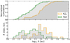 |
Fig. 2 Histograms and cumulative distributions of the radii enclosing 68% of the total CO and dust continuum emission for the Lupus disks that have measurements of the two sizes. Upper limits of the RCO and Rdust are included in the histograms, their value being the 95% confidence level. |
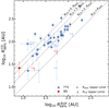 |
Fig. 3 Comparison between the R68% CO and dust emission for the entire disk population. |
5 Discussion
In this section, we discuss the physical implications of the CO and dust continuum sizes that we found for the entire Lupus disk population. Additionally, thanks to the significant number of disks with measured CO and dust sizes, we searched for possible correlations between the measured size ratio of the sample and various stellar and disk properties.
5.1 Disk evolution: gas size relative to dust size
The relativesize between gas and dust is a fundamental property of protoplanetary disks, since it can be linked to evolutionary processes of the disk (e.g., Dutrey et al. 1998; Facchini et al. 2017; Trapman et al. 2019). If the disk has undergone dust evolution (understood as grain growth and subsequent radial drift), the dust emission at (sub-)mm wavelength may appear much more compact than the gas emission. Gas evolution, on the other hand, cannot be constrained based only on the relative gas-dust size ratio. The two main mechanisms of angular momentum transport (viscous evolution, wind-driven accretion) generally cause the gaseous disk to either increase in size or remain similar; thus, the two mechanisms contribute to a large gas-dust size ratio if dust evolution has occurred.
A second major effect that contributes to the observed size divergence between gas and dust is the optical depth. This effect is due to the larger optical depth of the 12CO rotational line with respect to the continuum emission at (sub-)mm wavelengths. This causes the line emission to appear more extended than the optically thinner dust emission. Another way to understand the optical depth effect is by assuming a disk where gas and dust are equally distributed. If the dust emission is optically thin, the  would trace the 68% of the total disk mass. However, the R68% of an optically thick line would trace a larger fraction of the total disk mass, since the line emission from the innermost region is hidden due to the optical thickness. Thus, the measured
  of the optically thick line would necessarily be larger than the
  .
.
The presence of pressure bumps might also have an influence on the size ratio of a disk. If present, radial drift would stop at the location of the outermost bump, resulting in piled up dust and likely a ring-like structure. Although very high sensitivity and resolution observations are needed in order to confirm the presence of bumps or rings, most of the Lupus disks targeted on the DSHARP project show rings or enhancements of dust emission (Huang et al. 2018). The existence of bumps might cause dust sizes to be larger, resulting in smaller size ratios. The existence of bumps does not necessarily produce small size ratios: it would ultimately depend on the location of the bump.
As a result, disentangling between dust evolution and optical effect is very difficult: while the optical depth is almost certainly present, the dust evolution does not necessarily occur. Trapman et al. (2019) studied, in detail, the possible contributions of these andother effects to the gas-dust size ratio based on a large grid of thermo-chemical models (Facchini et al. 2017), and concluded that a size ratio higher than 4 is a clear sign of dust evolution. For disks below this threshold, dust evolution could still have occurred, but specific modeling of each disk is required in order to confirm it. In their study, the same radius definition as in the present work was used (a fraction of the total observable flux, not a physical radius), and their CO radii were obtained by measuring the flux extent of the same CO line (12 CO J =2−1), with differences in the CO sizesbelow 10% when considering the 12CO J =3−2 line. Therefore, their findings can be directly applied to our size ratio measurements. The population’s mean value of 2.5 that we obtain is farbelow the ratio threshold of 4 suggested by Trapman et al. (2019), thus radial drift cannot be confirmed as a ubiquitous process of the Lupus disk population. The threshold value of 4 might change slightly with a different setup of the thermo-chemical modeling. In Trapman et al. (2019), the threshold was obtained for a standard disk with a number of assumptions(most significantly, the gas structure being set by a self-similar solution of a viscous accreting disk, and a local gas-to-dust ratio of 100).
The fraction of disks with size ratios above the threshold value of 4 is ~15% for the entire population ( ~13% if we only consider disks of which the size ratio uncertainties are strictly above 4). If we examine the 0.7–1.1 M⊙ subsample, the fraction is marginally higher, with two out of nine objects (or one out of nine if only objects in this mass range with size ratio uncertainties above 4 are considered). These fractions of disks above the threshold remain the same if the R90% radii are used instead of R68% for the entire disk population and for the 0.7–1.1 M⊙ subsample. Following Trapman et al. (2019) results, these disks with size ratios above the threshold can only be explained if dust evolution took place.
The sources that we identified as having size ratios above the threshold of 4 are (from highest to lowest) Sz 75, Sz 131, Sz 69, Sz 83, Sz 65, and Sz 111. Although this subset of sources is small, the main stellar and disk properties cover relatively wide ranges; for instance, the stellar masses are distributed throughout 0.2 and 0.8 M⊙ .
In Appendix F, we describe each of these systems with high size ratios in detail. Sz 83, one of the most active sources of the Lupus clouds, might have a lower size ratio when considering the dynamical size based on Keplerian motion (Huang et al. 2020). On the other hand, for Sz 69 we only provide a lower bound since the size of the dust emission cannot be accurately determined. We did not find any properties or features that these disks might share: specifically, their accretion signatures are ordinary (Alcalá et al. 2017), and only one of them is a known transition disk (Sz 111 disk, van der Marel et al. 2018). Three of these disks belong to wide binary systems, at separations at which tidal truncation effects should not have any incidence.
In summary, ~ 15–20% of the disk population in Lupus has a disk size ratio greater than 4. This result suggests that a considerable fraction of protoplanetary disks in Lupus have suffered radial drift and dust evolution, which is crucial to form the cores of planets.
5.2 Possible correlations between the size ratio and other stellar and disk properties
The large population of disks with characterized CO and dust sizes allowed us to search for possible correlations between the CO-dust size ratio and the main stellar and disk properties. We examined the relation between the size ratio and the stellar mass, the total disk mass, and the dust and CO sizes separately. Figure 4 shows the size ratio as a function of each of these properties. The stellar mass and its uncertainty were obtained as explained in Sect. 2, while for the CO and dust sizes and uncertainties, we used the results from the modeling described in Sect. 3 (sizes summarized in Table 2). The total disk mass is approximated from the dust disk mass, assuming a gas-to-dust ratio of 100. The dust disk mass was computed assuming that the emission is optically thin and in the Rayleigh-Jeans regime (Beckwith et al. 1990), with an average temperature on the dust mid-plane of 20 K (as in Pascucci et al. 2016; Ansdell et al. 2016, 2018; Sanchis et al. 2020) and a dust optical depth of κ890 μm = 2 cm2 g−1 (as in Ricci et al. 2014; Testi et al. 2016; Sanchis et al. 2020). The uncertainty considered for the Mdust is the 10% associated with the flux calibrator uncertainty of the ALMA observations. The inferred Mdust values of each disk are included in Table 2. While this is a big approximation for the disk mass, it is useful in order to have an overall understanding of the available disk mass.
For this examination, we made use of the Spearman and Pearson correlation coefficients (similar to the analysis of dust property correlations conducted in Hendler et al. 2020). The Spearman test measures the monotonicity of the relationship between two sets of variables (its null hypothesis is that the two sets are monotonically uncorrelated), while the Pearson testevaluates the linear relationship between the two sets (its null hypothesis being that the two sets are linearly uncorrelated). The Pearson test assumes that the two variables are normally distributed. Therefore, we also tested the normality of each disk property by performing the Shapiro-Wilk test (Shapiro & Wilk 1965), of which the null hypothesis is that the set of values is drawn from a normal distribution. The scipy.stats Python module3 was used to perform the aforementioned tests. For each relationship, the tests were performed by excluding all objects with upper limits in the CO size or the dust size. If the p-value of a given test is below 0.05, the null hypothesis of the respective test was rejected.
The results of the tests are summarized in Table 3. The size ratio of the sample is not normally distributed since the null hypothesis of the Shapiro-Wilk test is rejected. Therefore, we cannot test for linearity between the size ratio and the other properties. However, the Spearman test can be performed independently of the normality of the properties. The relation between the size ratio and the Rdust is the only one that rejects the null hypothesis of the Spearman test, that is, it is unlikely that the size ratio and the Rdust are monotonically uncorrelated. Additionally, the measured size ratio of compact disks (those with sizes of the order of the beam size) may be lower than the true value due to the beam size (Trapman et al. 2019). In such cases, the anticorrelation with Rdust might be steeper than what isseen in Fig. 4. However, this result should be taken with caution, since the Y-axis (the size ratio) is dependent on the X-axis (Rdust is the denominator in the size ratio), thus the anticorrelation found could be boosted by this dependence between the two axes. Besides, the test does not take into account uncertainties, which are large in the Y-axis. If the anticorrelation with Rdust is true, it would mean that compact dusty disks have higher size ratios than extended dusty disks. Furthermore, if we consider the findings of Trapman et al. (2019), radial drift and dust evolution might be more prominent in these compact dusty disks. The Spearman test finds no monotonicity between the size ratio and RCO, thus the size ratio is more tightly affected by the dust size than the CO size. For the remaining properties (i.e., stellar and disk masses), no correlations are found.
The results plotted in Fig. 4 show that disks with very large size ratios (e.g., above the threshold considered) appear along the full range of stellar masses, disk masses, and CO sizes. These disks with exceptionally high size ratios may be in a different evolutionary stage compared to the bulk of the disk population. Therefore, we performed the correlation tests excluding disks with size ratios above the considered threshold of 4. The results of the different tests are summarized in the bottom rows of Table 3. Based on the Shapiro test, the size ratio of this subsample is normally distributed, thus the Pearson test can be performed. In this subsample, the tests yield a very low likelihood that the size ratio is uncorrelated with the dust size, analogous to the results for the entire sample. The tests do not confirm possible correlations with the remaining properties, although the p-value of the Spearman and Pearson’s tests between the size ratio and the stellar mass are very low (0.06 and 0.07). This result might point toward a possible anticorrelation with M⋆ . Based on the results of Trapman et al. (2019), this would tentatively suggest that dust evolution could be more efficient in disks around less massive stars. This is in line with theoretical and observational work that suggested radial drift is more effective in disks around low-mass stars (Pinilla et al. 2013; Pascucci et al. 2016; Mulders et al. 2015). In order to confirm or refute a tentative anticorrelation with M⋆ , it is necessary to significantly increase the sample of disks with measured gas and dust sizes.
The results of these statistical tests show a remarkable lack of strong correlations between the size ratio and the investigated properties. The sample of disks with measured size ratios is considerable, and it covers a very wide range of stellar masses, disk masses, dust, and CO sizes. And yet, the vast majority of the disks have similar ratios: between ~ 2 and 4. This denotes that, aside from the small fraction of disks with exceptionally high size ratios, the bulk of the population behaves in a similar manner, independent of its stellar and disk properties. Extending the sample of disks with characterized gas and dust sizes is essential to confirming our results. In particular, by expanding over other SFRs, the evolution of the size ratio over time can be investigated: this would help us to further constrain the ongoing and/or suffered physical processes and the evolutionary stage of the disks.
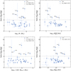 |
Fig. 4 Ratio between CO and dust sizes as a function of various stellar and disk properties. Top left: as a function of the stellar mass of the central object (M⋆ ).
Top right: asa function of the dust size ( |


Results of the statistical tests searching for possible correlations between the size ratio and various stellar and disk properties (M⋆, Mdisk , Rdust , and RCO ).
5.3 Optically thick emission and CO temperature
Lastly, we investigated the CO emission as a function of the CO size and tried to constrain the temperature of the CO-emitting layer. Figure 5 shows the modeled CO flux plotted against the CO size for the entire sample. First, we performed statistical tests (as in Sect. 5.2) searching for possible correlations between the two properties. The Spearman test provides a very low p-value (of 3e-5, obtained by excluding CO size upper limits). Therefore, its null hypothesis is rejected, and the two properties are monotonically correlated. On the other hand, linearity could not be tested since the CO flux sample is not normally distributed (its p-value from the Shapiro test is < 0.05). The monotonic correlation found is expected due to the optically thick emission of the 12CO lines.
Based on this result, it is also possible to examine the temperature of the CO emitting layer. In Fig. 5, we plot an orange line representing optically thick emission with an average CO temperature (TCO) of 30 K. This line is composed of a grid of optically thick emission profiles with a constant temperature. These profiles are constant with the radius and are thus described as ICO(R) = Bν(TCO), with ν being the frequency of the 12CO (J = 2−1) transition line, and TCO = 30 K. This TCO is based on the results of Pinte et al. (2018), where the emission profile of the same CO line (among dust continuum and other transition lines) was studied in detail for the IM Lup disk. The grid of profiles was assembled by taking increasing values of the outer disk edge, in order to cover the entire X-axis and populate the plot. For each profile, we computed the radius enclosing the 68% of the total intensity, and by plotting all the profiles we obtain the orange line.
In the figure, a disk with optically thick emission and an average TCO = 30 K would be intersected by this line. Around one third of the sample is crossed by this line when considering their uncertainties in radius. Considering only systems of which the errorbars do not cross the line, four disks lie on the left side of the optically thick line: one disk (Sz 72) is among the faintest disks of the sample, and its size uncertainty is large. This source, together with two other objects on the left side (Sz 73, Sz 102), can be explained either by an underestimation of their CO size, a higher CO temperature, or a combination of both. From the CO emission maps, these disks have abright compact core of emission (thus, likely warmer than 30 K), and their outer disk emission is either faint or absent. This could happen if the outer emission is fainter than the sensitivity of the observations. For the last source on the left side of the line (EX Lup), the presence of a blueshifted molecular outflow (Hales et al. 2018)makes the determination of the CO disk flux and size difficult, thus its exact position in the plot is uncertain.
On the other hand, a considerable fraction of the population appears on the right side of the optically thick line at 30 K (about half of the sample, only considering disks with errorbars not crossing the line). This can be explained by several factors. Firstly, cloud absorption, which can be seen in the line spectrum in a considerable number of disks (see Appendix E) can explain disks on the right side of the line. Absorption from clouds would decrease the total CO emission, while the measured radius would be mostly unaffected (Ansdell et al. 2018). Another possible explanation is that the average CO temperature of some of these disks could be below 30 K, which would be expected in very extended sources since the regions further from the star are generally colder. Besides this, the inclination of the disks might also have an effect. The optically thick line plotted assumes a face-on orientation: if inclined, the emission would appear fainter (the optically thick lines would shift downwards). Nevertheless, the CO fluxes of the Lupus disks shown in Fig. 5 are corrected accounting for the disk inclination, thus this effect should be minor. Lastly, partially optically thick CO emission in the outer disk can cause the emission to be fainter, thus appearing below the optically thick line.
A second line representing optically thick emission at the typical freeze-out temperature of CO (TCO = 20 K) is included in the figure. Eight disks appear on the right side of the 20 K line, taking errorbars into account. These disks are likely explained by a combination of the aforementioned effects that shift the position of the disk to the right side of the line. However, it might be possible that the CO in some regions of these disks is indeed at temperatures lower than the freeze-out temperature, which could be explained by vertical mixing, as suggested in Piétu et al. (2007).
For the case of the three BDs in the sample, their radii were obtained from a different CO transition (12 CO 3–2). The optically thick lines of the transition used for the BDs would appear slightly above the drawn lines of Fig. 5. The only BD with a measured size lies within errorbars on the 30 K line.
In conclusion, a monotonic correlation between the CO size and flux is found, as expected from optically thick emission. Our results for the temperature of the CO emitting layer are consistent with a temperature of around 30 K as previous studies suggested, albeit a fraction of the sample might have slightly lower average temperatures. However, the exact determination of TCO for the sample or for individual sources is difficult due to the size uncertainties, cloud absorption, and other factors that limit this analysis.
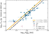 |
Fig. 5 Relation between the radius enclosing 68% of the total CO flux (scaled at the median distance of the region, and deprojected with inclination) and the flux enclosed by that radius for the entire Lupus CO disk population. Lines represent optically thick emission of CO with an average temperature of 30 (orange) and 20 K (black dash-dotted). Objects with outflows within the measured radius are considered to be upper limits in FCO . |
6 Conclusions
We investigated the relative extent of gas and dust in a large sample of protoplanetary disks of the Lupus clouds in order to constrain the evolutionary stage of the disk population. We assembled the largest sample of protoplanetary disks of the region with characterized CO and dust sizes based on ALMA observations. To infer the gas disk sizes, we modeled the integrated emission maps of the 12CO (J = 2−1) transition line from ALMA Band 6 observations using an elliptical Gaussian function, or a Nuker profile for models with considerable residuals. For the dust modeling, the continuum emission of large grains (at ~0.89 mm wavelength) was modeled in the uv-plane to a Nuker profile. The radii enclosing 68, 90, and 95% of the respective total flux, are estimated from the CO and dust models. The CO-dust size ratio (RCO/Rdust) was then used to investigate the evolutionary stage of the disk population; prominent dust evolution (i.e., grain growth and radial drift) typically produces compact dust emission at these wavelengths, and thus high size ratios. Gas evolution, on the other hand, cannot be constrained based only on this size ratio.
The median value of the size ratio is 2.5 for the entire population and for a subsample with high completeness. Fifteen percent of the population shows a size ratio above 4 (20% when considering a subsample with high completeness), based on thermo-chemical modeling (Facchini et al. 2017; Trapman et al. 2019), such high values can only be explained if grain growth and subsequent radial drift has occurred. These disks with very high size ratios do not show unusual characteristics, and their stellar and disk properties cover wide ranges of the entire population. For the rest of the population, dust evolution cannot be ruled out, but individual thermo-chemical modeling is necessary.
We searched for possible correlations of the population’s size ratio with other stellar and disk properties. Only a tentative monotonic anticorrelation with Rdust is suggested by the null hypothesis tests performed. The absence of strong correlations is very significant, the studied sample covers a wide range of stellar and disk properties, and the vast majority of the population has a very similar size ratio (between ~ 2 and 4). This suggests that a large fraction of protoplanetary disks in Lupus behave similarly and may be in a similar evolutionary stage. These results are limited by the optical depth difference between continuum and 12CO (J = 2−1) line, which can affect each disk’s measured size ratio differently, thus hiding its true behavior. Additionally, extending this analysis to the disk population in other SFRs is pivotal to learn about the temporal evolution and the evolutionary stages of protoplanetary disks. Finally, a monotonic correlation between the CO disk flux and size is found. The CO temperature for most of the disks, although difficult to determine accurately, is consistent with previous studies that suggest an average temperature of around 30 K.
Acknowledgements
We thank the anonymous referee for providing constructive comments that helped to improve the clarity and quality of the manuscript. This paper makes use of the following ALMA data: ADS/JAO.ALMA#2017.1.01243.S, ADS/JAO.ALMA#2013.1.00220.S, ADS/JAO.ALMA#2013.1.00226.S, ADS/JAO.ALMA#2013.1.00663.S, ADS/JAO.ALMA#2013.1.00694.S, ADS/JAO.ALMA#2013.1.00798.S, ADS/JAO.ALMA#2013.1.01020.S, ADS/JAO.ALMA#2015.1.00222.S, ADS/JAO.ALMA#2016.1.00484.L, and ADS/JAO.ALMA#2016.1.01239.S. ALMA is a partnership of ESO (representing its member states), NSF (USA) and NINS (Japan), together with NRC (Canada) and NSC and ASIAA (Taiwan) and KASI (Republic of Korea), in cooperation with the Republic of Chile. The Joint ALMA Observatory is operated by ESO, AUI/NRAO and NAOJ. This work was partly supported by the Italian Ministero dell Istruzione, Università e Ricerca through the grant Progetti Premiali 2012 – iALMA (CUP C52I13000140001), by the Deutsche Forschungs-gemeinschaft (DFG, German Research Foundation) - Ref no. FOR 2634/1 TE 1024/1-1, and by the DFG cluster of excellence Origins (www.origins-cluster.de). This project has received funding from the European Union’s Horizon 2020 research and innovation programme under the Marie Sklodowska-Curie grant agreement No 823823 (DUSTBUSTERS) and from the European Research Council (ERC) via the ERC Synergy Grant ECOGAL (grant 855130). S.F. acknowledges an ESO Fellowship. T.H. acknowledges support from the European Research Council under the Horizon 2020 Framework Program via the ERC Advanced Grant Origins 83 24 28. IdG-M is partially supported by MCIU-AEI (Spain) grant AYA2017-84390-C2-R (co-funded by FEDER). K.M. acknowledges funding by the Science and Technology Foundation of Portugal (FCT), grants No. IF/00194/2015, PTDC/FIS-AST/28731/2017 and UIDB/00099/2020.
Appendix A Interferometric modeling of DSHARP line emission
While analysis in the image plane gives first-order insightful information of the emission, fitting the observations in the uv-plane provides themost robust method to characterize the disk emission. By working in the uv-plane, we avoid systematic errors from the image reconstruction process (e.g., dependency on the weighting, and masking applied during this process).
In recent work, interferometric modeling made it possible to characterize dust continuum in large samples of disks from ALMA observations (e.g., Tazzari et al. 2017; Tripathi et al. 2017; Andrews et al. 2018b; Sanchis et al. 2020). We explored this methodology to model the line emission.
The interferometric modeling of the gas could be accomplished by integrating all channels that show disk emission after the continuum is subtracted. This is analogous (except in the Fourier space) to the moment zero map in which all the channel maps are summed up. The resulting visibilities can then be modeled to an empirical emission function, analogous to the interferometric modeling of dust continuum conducted by Sanchis et al. (2020).
Gas lineemission can be modeled using any preferred empirical function, in this work we used the Nuker function (for details of this function, see Tripathi et al. 2017) fit in the uv-plane as the fiducial CO sizes of these objects. The advantage of using this profile resides in independently fitting the inner and outer slopes of the disk emission. In Sect. 3.1.2, we also tested the interferometric modeling by fitting a Gaussian function (as Eq. (2) in Sanchis et al. 2020). This methodology assumes an axisymmetric emission of the disk, thus substructure or asymmetries are not modeled. Nevertheless, the size determination is not affected by the presence of substructure. More elaborated functions that account for these second-order features can be used on the interferometric modeling described here.
The Galario package (Tazzari et al. 2018) was used to convert the empirical model into synthetic visibilities, and to compute the χ2 between observed and synthetic visibilities. In addition, the affine invariant MCMC method from Goodman & Weare (2010) was also used (via the emcee package Foreman-Mackey et al. 2013) to investigate the parameter space, optimizing for models with the lowest χ2 . This was done for 200 independent walkers for thousands of steps. After a number of steps, the values of the free parameters converge to those that provide the best fit between synthetic and observed visibilities. Due to expensive computation time required to model the large set of visibilities from DSHARP observations, baselines > 1000kλ were excluded from the fit.
As an example, in the following figures of this appendix we present the results of the interferometric modeling of the Sz 71 CO disk fitted to a Nuker model. The fitting tool converges to the models with lowest χ2 . In Fig. A.1, we show the fit of the visibilities: real and imaginary part of observed and synthetic (for the model with lowest χ2 ) visibilities as a function of baseline.
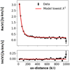 |
Fig. A.1 Observed and model visibilities of Sz 71 CO emission, plotted as real and imaginary parts as a function of the baseline (in kλ). The data from the observations are plotted as black data points with error bars, the model with the lowest χ2 is shown as solid red curve, and a random set of converged models from the parameter space investigation are drawn as gray curves (mostly covered by the lowest χ2 model). This figure was made with the uvplot Python package (Tazzari 2017). |
Once the fitting tool has converged, the subsequent MCMC method chains store the values of the parameters that fit best to the observed visibilities. Histograms of the free parameters were built from these chains. The median of each parameter’s histogram was taken as the best value of the parameter, and the 16th and 84th percentiles were used as lower and upper uncertainties. The 1D and 2D histograms between model parameters are plotted in Fig. A.2.
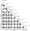 |
Fig. A.2 Corner plot of the Nuker fitting of the observed CO visibilities. Top subpanels: histograms of the free parameters from the MCMC chains. The remaining subpanels show the 2D histograms between pairs of parameters. |
Additionally, in order to have an idea of the quality of the interferometric modeling, we show the observed, modeled, and residual moment zero maps of CO reconstructed from the visibilities in Fig. A.3. In order to visualize the differences between the Nuker modeling and the Gaussian modeling in the uv-plane, we also include the reconstructed maps of the Gaussian fit in Fig. A.3.
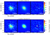 |
Fig. A.3 Reconstructed moment zero maps from fitting, in the uv-plane, the observed CO emission around GW Lup (Sz 71) using a Nuker profile model (top panels) and an elliptical Gaussian function (bottom panels). For each model, the subpanels represent the observed (left), modeled (center) and residual (right) reconstructed CO maps. |
The cumulative distribution function (fcumul) for each model was built from the converged chains. From the cumulative distribution, we estimated the R68%, R90%, and R95% CO radii of eachmodel, and built histograms of each radius. The main value and lower and upper uncertainties of each radius are the median 16thand 84th percentiles of the respective histograms. The cumulative distribution and mean radii values for the modeled CO disk of Sz 71 are shown in Fig. A.4.
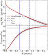 |
Fig. A.4 Radial brightness profile (top panel) and the associated cumulative flux (bottom panel) modeled for the CO emission of Sz 71 fit to a Nuker profile. The emission distribution of the model with lowest χ2 from the fit is drawn as red, while a subset of converged models are shown as thin gray curves. |
The CO radii results from the interferometric modeling (fitting a Nuker and a Gaussian function) of all the DSHARP disks can be found in Table B.1. The Sz 68 CO disk was excluded from the interferometric modeling since it is part of a multiple system that is unresolved in the Lupus disk survey. Additionally, the CO integrated emission from the DSHARP survey is irregular: its shape does not resemble a smooth disk.
Appendix B Results of CO sizes using different methodology
In this appendix, we summarize the CO radii obtained by different modeling (Table B.1) for the two datasets (Lupus disk survey, and DSHARP project). The different models considered are the interferometric modeling of the DSHARP visibilities fitting Nuker and Gaussian functions, the elliptical Gaussian modeling in the image plane for the two datasets, and the Nuker fit in the image plane for the lower sensitivity and resolution dataset. These results were used to assess the systematic uncertainties of the modeling described in Sect. 3.1.
Lastly, in Fig. B.1, we compare CO radii obtained from the elliptical Gaussian modeling in the image plane of the lower sensitivity dataset (as described in Appendix A) with the CO radii from the interferometric fit of a Nuker modeling of the DSHARP data (explained in Appendix A) for the same objects. The radii based on the interferometric modeling of the DSHARP data were considered as the fiducial CO sizes of the disks. This comparison was used in Sect. 3.1.2 to assess the quality of the elliptical Gaussian modeling.
CO radii of protoplanetary disks in Lupus observed in the DSHARP survey, inferred from modeling in the image and in the uv-plane, using two different datasets (Lupus disk survey, and DSHARP observations).
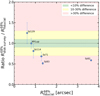 |
Fig. B.1 Comparison between the CO radial extent of objects with two datasets (Lupus disk survey and DSHARP project). The Y-axis shows the ratio between the radius from the Lupus disk survey (obtained by fitting an elliptical Gaussian model in the moment zero map) divided by the fiducial radius of the CO disk. The fiducial CO size is considered as the size inferred from the DSHARP dataset by interferometric fitting of the line visibilities with a Nuker model (interferometric modeling described in Appendix A). The X-axis represents the fiducial size to ease the comparison. The colored regions indicate disks with a divergence in sizes below 10% (green region), between and 10 and 30% (yellow), and greater than 30% (red). |
Appendix C Criterion for the CO modeling in the image plane based on the residuals
The residuals were quantified as the sum of emission enclosed by the inferred R68% and centered at the elliptical Gaussian centroid in the residual map. Absolute values were used to account for negative residuals. This quantity was also computed on the observed moment zero map centered on the object, and on an emission-free region of the sky (averaged over four random locations in the background). The following two quantities were used as the criteria for the quality of the fit: the residuals over background fraction  , and the difference between residuals and background over the observed disk emission
  . A value of 1 in the first quantity means that the residuals of the model are indistinguishable from the background emission. The second quantity gives an idea of the fraction of residuals over the observed disk emission; in this case, a 0 value represents a perfect model. These quantities were used together with the size ratio between the model and the fiducial size of each disk to evaluate the quality of each model. The results for elliptical Gaussian models are shown in the two subpanels of Fig. C.1 for those disks in which we have the two (moderate- and high-resolution) datasets. The red lines in both panels represent the median (μ) and μ ± σ for the entire Lupus CO disks sample of the respective quantity. For both quantities, the four disks within the region delimited by the μ ± σ region (Sz 71, Sz 114, Sz 129, and MY Lup) all have a size divergence with the fiducial CO size between 0 and ~ 30%. On the other hand, Sz 82 and Sz 83 fall clearly outside; these disks show a larger divergence in size, both having > 40% difference with respect to the fiducial size.
From this analysis, elliptical Gaussian modeling of disks with residuals within the μ ± σ range of the sample (as in Fig. C.1) provide CO sizes with an accuracy between 0 and ~ 30%. Gaussian models of disks with residuals outside the valid range can differ more than 40% with respect to the fiducial value. Therefore, for disks with residuals outside the μ ± σ, their CO emission should not be modeled with a Gaussian function, and instead we modeled their emission by fitting the integrated maps with a Nuker profile (as described in Sect. 3.1). We also tested the quality of the sizes inferred from the Nuker profile modeling in the image plane. The size ratio between the Nuker model in the image plane and the fiducial model is represented as a function of the Nuker model residuals in Fig. C.2. The results show that the inferred radii are in better agreement with the fiducial sizes than the Gaussian modeling. The size difference is found to be ~ 0−30% for every disk, and this remains true for the three radii (R68%, R90%, and R95%).
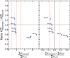 |
Fig. C.1 CO size ratio compared to the residuals from the elliptical Gaussian modeling for the six disks with two datasets available. The fiducial radii are the sizes obtained from the interferometric modeling of the visibilities from the DSHARP dataset, following the methodology described in Appendix A. Left panel: size ratio as a function of residuals over background fraction (criterion 1). Right panel: size ratio vs. the difference between residuals and background over the observed disk emission (criterion 2). The central redline represents the median value of the entire Lupus sample, left and right vertical lines are the μ ± σ values. |
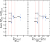 |
Fig. C.2 Criteria for residuals of Nuker modeling of the six disks with two datasets available. The fiducial radii are the sizes obtained from the interferometric modeling of the visibilities from the DSHARP dataset, following the methodology described in Appendix A. Left panel: size ratio as a function of residuals over background fraction (criterion 1). Right panel: size ratio vs. difference between residuals and background over the observed disk emission (criterion 2). Red verticallines identical to the ones in Fig. C.1. |
Appendix D Best-fit parameters for CO disks modeled with a Nuker function
Appendix E Observed, model, and residual CO maps of the Lupus disk population
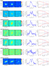 |
Fig. E.1 Results of the CO modeling for every disk with a measured CO size, following the methodology described in Sect. 3.1. For each disk, the first three subpanels show the observed, model, and residual CO moment zero maps; solid (dashed) line contours are drawn at increasing (decreasing) 3σ intervals. Forth subpanel: integrated spectrum enclosed by the |

 |
Fig. E.1 continued. |
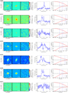 |
Fig. E.1 continued. |
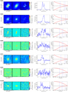 |
Fig. E.1 continued. |
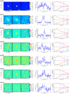 |
Fig. E.1 continued. |
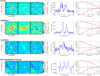 |
Fig. E.1 continued. |
Appendix F Singular objects
In this section, we discuss unusual systems in the Lupus sample, namely, outliers of the size ratio distribution, or those with particular known features.
F.1 Sz 75
The Sz 75 system (or GQ Lup) has a central star of 0.8 M⊙ , a sub-stellar companion at an angular separation of ~0.7′′ (Neuhäuser et al. 2005) of uncertain mass (likely in the BD regime, Seifahrt et al. 2007; Neuhäuser et al. 2008; Lavigne et al. 2009), and a second companion candidate at 16′′ of ~ 0.15 M⊙ that is likely gravitationally bound to the central object (Alcalá et al. 2020). The first companion is within the pointing of the ALMA observations, but no 12CO or continuum emission is detected around it. The second companion candidate falls outside the ALMA pointing, however, its disk was detected in archival HST and WISE data (Lazzoni et al. 2020).
The disk of the central star has the largest size-ratio of the entire Lupus population (size ratio of ~ 8). Previous ALMA observations (MacGregor et al. 2017; Long et al. 2020), yielded consistent results of the 12CO (3–2) and dust continuum extent. The compact continuum emission together with the large size ratio confirms that radial drift has been particularly efficient in the disk around the central star. Whether the presence of companions has boosted the radial drift process is unknown, follow-up studies on this system are needed in order to address this question.
The CO disk around the central star (with  = 1.7′′) extents beyond the deprojected distance between central star and the sub-stellar companion, considering the companion’s orbital inclination to be ~60° as suggested by Schwarz et al. (2016). This is contrary to expected tidal truncation effects (e.g., Martin & Lubow 2011; Bate 2018), possibly due to the sub-stellar nature of this companion. Additionally, the CO channel maps do not show any distortion due to the presence of the sub-stellar object.
The formation mechanism of the system is unclear. A possible scenario, suggested by Alcalá et al. (2020), is that the central star and the second companion might be formed by fragmentation of a turbulent core. Likewise, the formation of the primary companion is uncertain (MacGregor et al. 2017): if due to fragmentation of the circumprimary disk, it would result in a relatively massive disk around the sub-stellar companion; while formation close the central star and posterior scattering outwards is a less favored explanation (Bryan et al. 2016).
F.2 Sz 83
This source (also known as RU Lup) is one of the most active young stars of the Lupus clouds (Comerón 2008). The CO-dust size ratio measured is very large (≃5). However, the result should be taken with caution, since the structure of this disk is highly complex, with outflows, jets and mild cloud contamination (Herczeg et al. 2005; Ansdell et al. 2018; Andrews et al. 2018a).
Recent high-angular-resolution observations of the 12CO, 13CO, C18CO, and DCO+ lines showed an intricate structure of the gas in this system, with a central Keplerian disk, an extended diffuse emission, spiral arms, and various “clumps” of emission (Huang et al. 2020). The CO size reported in that work distinguishes between a Keplerian disk of ~ 0.75′′, non-Keplerian CO emission of ~ 1.6′′, spiral structure up to ~ 6′′ , and clumps further out. Although they did not report values of R68%, our R95% is slightly larger than the non-Keplerian emission reported in Huang et al. (2020). Since our measurement considers any detected emission (from the 12CO J =2−1 line observed from the ALMA Band 6 Lupus disk survey), our size likely accounts for part of the spiral structure.
However, the difference between the gas and the dust size is expected to be large, based on the recent studies of the system (e.g., Huang et al. 2020), and, in addition, our dust size coincides with previous works (e.g., Andrews et al. 2018b; Hendler et al. 2020). For consistency, we used our inferred CO size throughout this manuscript, but we warn that, due to the complexstructure of this system, the true extent of the CO disk might differ with respect to our tabulated values.
F.3 Sz 131
This is a single star system (0.3 M⊙ mass) and has as well a very high size ratio (~7.2), although with high uncertainty. The large size ratio is driven by the very compact continuum emission, of only 0.08′′. The high uncertainty is caused by the very faint emission in both 12CO and continuum, resulting in large error bars of the RCO and Rdust sizes. Even considering the upper bound of the dust size and the lower bound of the CO size, the ratio lies above 4, providing strong evidence of dust evolution and radial drift.
F.4 Sz 111
The Sz 111 system is another single star (of 0.5 M⊙ mass) with a bright disk in both continuum and 12CO. Its size ratio is slightly above the threshold of 4, dominated by the CO disk extent, which is among the largest CO disks of the Lupus population ( = 2.1 ± 0.4′′). Due to its extended emission in both CO and dust continuum, this system is a good candidate for future ALMA observations at higher resolution and sensitivity to better constrain the radial drift, and to resolve possible substructures as the aftermath of dust evolution.
F.5 Sz 69
The Sz 69 (HW Lup) system is part of a wide visual binary together with 2MASS J15451720-3418337, a source in the southwestern direction at ~6.6′′ of angular separation (Merín et al. 2008). The second element of the binary is non-detected both in dust continuum and CO.
The dusty disk around Sz 69 is extremely compact and partially unresolved, with an  . Due to its compact continuum emission, the CO-dust size ratio is particularly high, with a lower bound value of 5.7. Using the dust disk size from Andrews et al. (2018b), the size ratio would be 9.3. Such a high value of the size ratio points toward extremely efficient radial drift. The angular separation between the binary components is larger than the distances at which dynamical interactions would typically alter the circumprimary disk (e.g., Jensen et al. 1996; Bate 2000; Harris et al. 2012). A better characterization of the second source is necessary in order to understand this system in more detail.
F.6 Sz 65
The disk around Sz 65 (0.7 M⊙ ) has a size ratio of 4.8, and it is therefore another disk with a ratio above the threshold value of 4. It forms a binary system together with Sz 66 (0.3 M⊙ ), with an angular separation of ~ 6.4′′. The disk around the second component is very faint in both 12CO and dust continuum (with a size ratio of about 2.5), the size of the CO disk could not be constrained due to its compactness.
This is another multiple system in which the primary element has a very large size ratio, this case is particularly appealing since CO and dust are detected in the two components. Observations at a higher resolution and sensitivity level of the two components will significantly improve understanding the level of dust evolution of the two disks. Intriguingly, Sz 65’s accretion is weak and considered to be only an upper limit (its excess emission is close to the chromospheric levels, Alcalá et al. 2017), while accretion in Sz 66 is slightly above the known correlation with the continuum flux (see, e.g., Manara et al. 2016; Alcalá et al. 2017; Sanchis et al. 2020).
F.7 Sz 82
The Sz 82 (IM Lup) system is the brightest object of the entire Lupus disk population, both in 12CO and in dust continuum emission. It is therefore among the most studied protoplanetary disks. This disk is exceptionally large, its azimuthally averaged emission shows a plateau of emission that extends up to ≳ 1000 AU. Extensive modeling of several CO lines at scales <450 was performed by Pinte et al. (2018) and suggested that UV photo-desorption from the interstellar radiation field could explain the further out CO emission. In Cleeves et al. (2016), they discussed the possible origin of this diffuse emission: it could be the remnant of an envelope, a plausible explanation since the system is young (≤ 1 Myr, Mawet et al. 2012). Gravitationally captured gas is another viable scenario, since the system has a Bondi radius of ~ 3000 AU, far beyond the diffuse emission extent. Foreground emission is less likely since there is an offset between the cloud velocity and the object.
F.8 Brown dwarfs and very low-mass stars
We wish to highlight the results in the very low-mass range of the Lupus disk population; BDs are of particular interest since their formation and evolution might differ from disks around more massive stars. To do so, we only considered disks orbiting around objects of masses below 0.2 M⊙ . Several of these objects were targeted in a separate survey (Sanchis et al. 2020). Six disks in this mass range have inferred CO and dust sizes (Sz 84, Sz 100, Sz 114, SSTc2d J160703.9-391112, 2MASS J16081497-3857145, and SSTc2d J154518.5-342125). From theoretical modeling of the gas-dust size ratios (Trapman et al. 2019), the measured sizes inferred from the emission extent can be affected by the resolution of the observations, and in objects for which the emission extent is of the order of the beam size, the size ratios inferred could be lower than the true size ratios.
The median size ratio of disks around very low-mass stars is 3.1 (with a dispersion of 0.4), larger than the mean value of the entire population. If the low resolution/beam size effect is indeed affecting the inferred CO and dust sizes of these compact sources, the true size ratio may be even larger than the observed values. Due to the low number of sources in this range, it is not yet possible to address whether radial drift in disks around this mass range is more efficient than in disks around more massive stars, as predicted theoretically in Pinilla et al. (2013). It is also worth noting that the only BD in the sample with inferred sizes has a ratio of 3.2, which is higher than the median of the entire disk population. Due to the faint and compact emission of this source, its size uncertainties are relatively large, thus it is difficult to address the true behavior of this disk. Follow-up observationsof this source at higher resolution and sensitivity will allow us to better constrain its gas-dust size ratio.
References
- Alcalá, J. M., Natta, A., Manara, C. F., et al. 2014, A&A, 561, A2 [NASA ADS] [CrossRef] [EDP Sciences] [Google Scholar]
- Alcalá, J. M., Manara, C. F., Natta, A., et al. 2017, A&A, 600, A20 [NASA ADS] [CrossRef] [EDP Sciences] [Google Scholar]
- Alcalá, J. M., Manara, C. F., France, K., et al. 2019, A&A, 629, A108 [NASA ADS] [CrossRef] [EDP Sciences] [Google Scholar]
- Alcalá, J. M., Majidi, F. Z., Desidera, S., et al. 2020, A&A, 635, L1 [NASA ADS] [CrossRef] [EDP Sciences] [Google Scholar]
- Andrews, S. M. 2015, PASP, 127, 961 [NASA ADS] [CrossRef] [Google Scholar]
- Andrews, S. M., Wilner, D. J., Hughes, A. M., et al. 2012, ApJ, 744, 162 [Google Scholar]
- Andrews, S. M., Huang, J., Pérez, L. M., et al. 2018a, ApJ, 869, L41 [Google Scholar]
- Andrews, S. M., Terrell, M., Tripathi, A., et al. 2018b, ApJ, 865, 157 [Google Scholar]
- Ansdell, M., Williams, J. P., van der Marel, N., et al. 2016, ApJ, 828, 46 [Google Scholar]
- Ansdell, M., Williams, J. P., Manara, C. F., et al. 2017, AJ, 153, 240 [NASA ADS] [CrossRef] [EDP Sciences] [Google Scholar]
- Ansdell, M., Williams, J. P., Trapman, L., et al. 2018, ApJ, 859, 21 [Google Scholar]
- Avenhaus, H., Quanz, S. P., Garufi, A., et al. 2018, ApJ, 863, 44 [Google Scholar]
- Baraffe, I., Homeier, D., Allard, F., & Chabrier, G. 2015, A&A, 577, A42 [NASA ADS] [CrossRef] [EDP Sciences] [Google Scholar]
- Barenfeld, S. A., Carpenter, J. M., Ricci, L., & Isella, A. 2016, ApJ, 827, 142 [Google Scholar]
- Bate, M. R. 2000, MNRAS, 314, 33 [Google Scholar]
- Bate, M. R. 2018, MNRAS, 475, 5618 [Google Scholar]
- Beckwith, S. V. W., Sargent, A. I., Chini, R. S., & Guesten, R. 1990, AJ, 99, 924 [NASA ADS] [CrossRef] [Google Scholar]
- Birnstiel, T., Dullemond, C. P., & Brauer, F. 2010, A&A, 513, A79 [NASA ADS] [CrossRef] [EDP Sciences] [Google Scholar]
- Boyden, R. D., & Eisner, J. A. 2020, ApJ, 894, 74 [NASA ADS] [CrossRef] [Google Scholar]
- Bryan, M. L., Bowler, B. P., Knutson, H. A., et al. 2016, ApJ, 827, 100 [Google Scholar]
- Bustamante, I., Merín, B., Ribas, Á., et al. 2015, A&A, 578, A23 [NASA ADS] [CrossRef] [EDP Sciences] [Google Scholar]
- Canovas, H., Caceres, C., Schreiber, M. R., et al. 2016, MNRAS, 458, L29 [NASA ADS] [CrossRef] [Google Scholar]
- Cazzoletti, P., Manara, C. F., Baobab Liu, H., et al. 2019, A&A, 626, A11 [NASA ADS] [CrossRef] [EDP Sciences] [Google Scholar]
- Cieza, L. A., Ruíz-Rodríguez, D., Perez, S., et al. 2018, MNRAS, 474, 4347 [Google Scholar]
- Cleeves, L. I., Öberg, K. I., Wilner, D. J., et al. 2016, ApJ, 832, 110 [NASA ADS] [CrossRef] [Google Scholar]
- Comerón, F. 2008, The Lupus Clouds, ed. B. Reipurth, 295 [Google Scholar]
- Cox, E. G., Harris, R. J., Looney, L. W., et al. 2017, ApJ, 851, 83 [Google Scholar]
- Cutri, R. M., Skrutskie, M. F., van Dyk, S., et al. 2003, 2MASS All Sky Catalog of Point Sources [Google Scholar]
- Dunham, M. M., Allen, L. E., Evans, Neal J., I., et al. 2015, ApJS, 220, 11 [Google Scholar]
- Dutrey, A., Guilloteau, S., Prato, L., et al. 1998, A&A, 338, L63 [NASA ADS] [Google Scholar]
- Evans, Neal J., I., Dunham, M. M., Jørgensen, J. K., et al. 2009, ApJS, 181, 321 [Google Scholar]
- Facchini, S., Birnstiel, T., Bruderer, S., & van Dishoeck, E. F. 2017, A&A, 605, A16 [NASA ADS] [CrossRef] [EDP Sciences] [Google Scholar]
- Facchini, S., van Dishoeck, E. F., Manara, C. F., et al. 2019, A&A, 626, L2 [NASA ADS] [CrossRef] [EDP Sciences] [Google Scholar]
- Foreman-Mackey, D., Hogg, D. W., Lang, D., & Goodman, J. 2013, PASP, 125, 306 [Google Scholar]
- Fouchet, L., Maddison, S. T., Gonzalez, J. F., & Murray, J. R. 2007, A&A, 474, 1037 [NASA ADS] [CrossRef] [EDP Sciences] [Google Scholar]
- Frasca, A., Biazzo, K., Alcalá, J. M., et al. 2017, A&A, 602, A33 [NASA ADS] [CrossRef] [EDP Sciences] [Google Scholar]
- Gaia Collaboration (Brown, A. G. A., et al.) 2018, A&A, 616, A1 [NASA ADS] [CrossRef] [EDP Sciences] [Google Scholar]
- Garufi, A., Avenhaus, H., Pérez, S., et al. 2020, A&A, 633, A82 [CrossRef] [EDP Sciences] [Google Scholar]
- Goodman, J., & Weare, J. 2010, Commun. Appl. Math. Comput. Sci., 5, 65 [Google Scholar]
- Guilloteau, S.,& Dutrey, A. 1998, A&A, 339, 467 [NASA ADS] [Google Scholar]
- Hales, A. S., Pérez, S., Saito, M., et al. 2018, ApJ, 859, 111 [Google Scholar]
- Harris, R. J., Andrews, S. M., Wilner, D. J., & Kraus, A. L. 2012, ApJ, 751, 115 [NASA ADS] [CrossRef] [Google Scholar]
- Hendler, N., Pascucci, I., Pinilla, P., et al. 2020, ApJ, 895, 126 [Google Scholar]
- Herczeg, G. J., Walter, F. M., Linsky, J. L., et al. 2005, AJ, 129, 2777 [NASA ADS] [CrossRef] [Google Scholar]
- Huang, J., Andrews, S. M., Dullemond, C. P., et al. 2018, ApJ, 869, L42 [Google Scholar]
- Huang, J., Andrews, S. M., Öberg, K. I., et al. 2020, ApJ, 898, 140 [NASA ADS] [CrossRef] [Google Scholar]
- Hueso, R., & Guillot, T. 2005, A&A, 442, 703 [NASA ADS] [CrossRef] [EDP Sciences] [Google Scholar]
- Hughes, J., Hartigan, P., Krautter, J., & Kelemen, J. 1994, AJ, 108, 1071 [Google Scholar]
- Isella, A., Testi, L., Natta, A., et al. 2007, A&A, 469, 213 [CrossRef] [EDP Sciences] [Google Scholar]
- Jensen, E. L. N., Mathieu, R. D., & Fuller, G. A. 1996, ApJ, 458, 312 [Google Scholar]
- Lauer, T. R., Ajhar, E. A., Byun, Y.-I., et al. 1995, AJ, 110, 2622 [NASA ADS] [CrossRef] [EDP Sciences] [Google Scholar]
- Lavigne, J.-F., Doyon, R., Lafrenière, D., Marois, C., & Barman, T. 2009, ApJ, 704, 1098 [Google Scholar]
- Lazzoni, C., Gratton, R., Alcalá, J. M., et al. 2020, A&A, 635, L11 [NASA ADS] [CrossRef] [EDP Sciences] [Google Scholar]
- Long, F., Herczeg, G. J., Pascucci, I., et al. 2017, ApJ, 844, 99 [NASA ADS] [CrossRef] [Google Scholar]
- Long, D. E., Zhang, K., Teague, R., & Bergin, E. A. 2020, ApJ, 895, L46 [NASA ADS] [CrossRef] [Google Scholar]
- Lynden-Bell, D., & Pringle, J. E. 1974, MNRAS, 168, 603 [NASA ADS] [CrossRef] [Google Scholar]
- MacGregor, M. A., Wilner, D. J., Czekala, I., et al. 2017, ApJ, 835, 17 [Google Scholar]
- Manara, C. F., Rosotti, G., Testi, L., et al. 2016, A&A, 591, L3 [NASA ADS] [CrossRef] [EDP Sciences] [Google Scholar]
- Manara, C. F., Prusti, T., Comeron, F., et al. 2018, A&A, 615, L1 [NASA ADS] [CrossRef] [EDP Sciences] [Google Scholar]
- Martin, R. G., & Lubow, S. H. 2011, MNRAS, 413, 1447 [Google Scholar]
- Mawet, D., Absil, O., Montagnier, G., et al. 2012, A&A, 544, A131 [NASA ADS] [CrossRef] [EDP Sciences] [Google Scholar]
- McMullin, J. P., Waters, B., Schiebel, D., Young, W., & Golap, K. 2007, ASP Conf. Ser., 376, 127 [Google Scholar]
- Merín, B., Jørgensen, J., Spezzi, L., et al. 2008, ApJS, 177, 551 [Google Scholar]
- Miotello, A., van Dishoeck, E. F., Kama, M., & Bruderer, S. 2016, A&A, 594, A85 [NASA ADS] [CrossRef] [EDP Sciences] [Google Scholar]
- Miotello, A., van Dishoeck, E. F., Williams, J. P., et al. 2017, A&A, 599, A113 [NASA ADS] [CrossRef] [EDP Sciences] [Google Scholar]
- Mordasini, C., Alibert, Y., Benz, W., Klahr, H., & Henning, T. 2012, A&A, 541, A97 [NASA ADS] [CrossRef] [EDP Sciences] [Google Scholar]
- Mortier, A., Oliveira, I., & van Dishoeck, E. F. 2011, MNRAS, 418, 1194 [NASA ADS] [CrossRef] [Google Scholar]
- Mulders, G. D., Pascucci, I., & Apai, D. 2015, ApJ, 814, 130 [NASA ADS] [CrossRef] [Google Scholar]
- Mužić, K., Scholz, A., Geers, V. C., Jayawardhana, R., & López Martí, B. 2014, ApJ, 785, 159 [NASA ADS] [CrossRef] [Google Scholar]
- Mužić, K., Scholz, A., Geers, V. C., & Jayawardhana, R. 2015, ApJ, 810, 159 [Google Scholar]
- Najita, J. R., & Bergin, E. A. 2018, ApJ, 864, 168 [Google Scholar]
- Nakamoto, T.,& Nakagawa, Y. 1994, ApJ, 421, 640 [NASA ADS] [CrossRef] [Google Scholar]
- Neuhäuser, R., Guenther, E. W., Wuchterl, G., et al. 2005, A&A, 435, L13 [NASA ADS] [CrossRef] [EDP Sciences] [Google Scholar]
- Neuhäuser, R., Mugrauer, M., Seifahrt, A., Schmidt, T. O. B., & Vogt, N. 2008, A&A, 484, 281 [NASA ADS] [CrossRef] [EDP Sciences] [Google Scholar]
- Pascucci, I., Testi, L., Herczeg, G. J., et al. 2016, ApJ, 831, 125 [Google Scholar]
- Piétu, V., Dutrey, A., & Guilloteau, S. 2007, A&A, 467, 163 [NASA ADS] [CrossRef] [EDP Sciences] [Google Scholar]
- Pinilla, P., Benisty, M., & Birnstiel, T. 2012, A&A, 545, A81 [NASA ADS] [CrossRef] [EDP Sciences] [Google Scholar]
- Pinilla, P., Birnstiel, T., Benisty, M., et al. 2013, A&A, 554, A95 [NASA ADS] [CrossRef] [EDP Sciences] [Google Scholar]
- Pinte, C., Ménard, F., Duchêne, G., et al. 2018, A&A, 609, A47 [NASA ADS] [CrossRef] [EDP Sciences] [Google Scholar]
- Ricci, L., Testi, L., Natta, A., et al. 2014, ApJ, 791, 20 [NASA ADS] [CrossRef] [Google Scholar]
- Rosotti, G. P., Tazzari, M., Booth, R. A., et al. 2019, MNRAS, 486, 4829 [NASA ADS] [CrossRef] [Google Scholar]
- Sanchis, E., Testi, L., Natta, A., et al. 2020, A&A, 633, A114 [CrossRef] [EDP Sciences] [Google Scholar]
- Santamaría-Miranda, A., de Gregorio-Monsalvo, I., Huélamo, N., et al. 2020, A&A, 640, A13 [CrossRef] [EDP Sciences] [Google Scholar]
- Schwarz, H., Ginski, C., de Kok, R. J., et al. 2016, A&A, 593, A74 [NASA ADS] [CrossRef] [EDP Sciences] [Google Scholar]
- Seifahrt, A., Neuhäuser, R., & Hauschildt, P. H. 2007, A&A, 463, 309 [NASA ADS] [CrossRef] [EDP Sciences] [Google Scholar]
- Sellek, A. D., Booth, R. A., & Clarke, C. J. 2020a, MNRAS, 498, 2845 [CrossRef] [Google Scholar]
- Sellek, A. D., Booth, R. A., & Clarke, C. J. 2020b, MNRAS, 492, 1279 [CrossRef] [Google Scholar]
- Shapiro, S. S., & Wilk, M. B. 1965, Biometrika, 52, 591 [Google Scholar]
- Siess, L., Dufour, E., & Forestini, M. 2000, A&A, 358, 593 [Google Scholar]
- Tazzari, M. 2017, mtazzari/uvplot: v0.1.1 [Google Scholar]
- Tazzari, M., Testi, L., Natta, A., et al. 2017, A&A, 606, A88 [NASA ADS] [CrossRef] [EDP Sciences] [Google Scholar]
- Tazzari, M., Beaujean, F., & Testi, L. 2018, MNRAS, 476, 4527 [Google Scholar]
- Testi, L., Birnstiel, T., Ricci, L., et al. 2014, in Protostars and Planets VI, eds. H. Beuther, R. S. Klessen, C. P. Dullemond, & T. Henning (Tucson: University of Arizona Press), 339 [Google Scholar]
- Testi, L., Natta, A., Scholz, A., et al. 2016, A&A, 593, A111 [NASA ADS] [CrossRef] [EDP Sciences] [Google Scholar]
- Trapman, L., Facchini, S., Hogerheijde, M. R., van Dishoeck, E. F., & Bruderer, S. 2019, A&A, 629, A79 [NASA ADS] [CrossRef] [EDP Sciences] [Google Scholar]
- Trapman, L., Ansdell, M., Hogerheijde, M. R., et al. 2020, A&A, 638, A38 [NASA ADS] [CrossRef] [EDP Sciences] [Google Scholar]
- Tripathi, A., Andrews, S. M., Birnstiel, T., & Wilner, D. J. 2017, ApJ, 845, 44 [NASA ADS] [CrossRef] [Google Scholar]
- Turner, N. J., Fromang, S., Gammie, C., et al. 2014, in Protostars and Planets VI, eds. H. Beuther, R. S. Klessen, C. P. Dullemond, & T. Henning (Tucson: University of arizona Press), 411 [Google Scholar]
- van der Marel, N., Williams, J. P., Ansdell, M., et al. 2018, ApJ, 854, 177 [Google Scholar]
- van Dishoeck, E. F., & Black, J. H. 1988, ApJ, 334, 771 [Google Scholar]
- van Terwisga, S. E., van Dishoeck, E. F., Ansdell, M., et al. 2018, A&A, 616, A88 [NASA ADS] [CrossRef] [EDP Sciences] [Google Scholar]
- Weidenschilling, S. J. 1977, MNRAS, 180, 57 [Google Scholar]
- Williams, J. P., Cieza, L., Hales, A., et al. 2019, ApJ, 875, L9 [Google Scholar]
Using the scipy.optimize Python module: https://www.tutorialspoint.com/scipy/scipy_optimize.htm
Using the scipy.stats Python module: https://docs.scipy.org/doc/scipy/reference/stats.html
All Tables
Summary of archival ALMA projects used in this work for the gas and dust modeling.
Results of the statistical tests searching for possible correlations between the size ratio and various stellar and disk properties (M⋆, Mdisk , Rdust , and RCO ).
CO radii of protoplanetary disks in Lupus observed in the DSHARP survey, inferred from modeling in the image and in the uv-plane, using two different datasets (Lupus disk survey, and DSHARP observations).
All Figures
|
Fig. 1 Left panel: comparison between |
| In the text | |
|
Fig. 2 Histograms and cumulative distributions of the radii enclosing 68% of the total CO and dust continuum emission for the Lupus disks that have measurements of the two sizes. Upper limits of the RCO and Rdust are included in the histograms, their value being the 95% confidence level. |
| In the text | |
|
Fig. 3 Comparison between the R68% CO and dust emission for the entire disk population. |
| In the text | |
|
Fig. 4 Ratio between CO and dust sizes as a function of various stellar and disk properties. Top left: as a function of the stellar mass of the central object (M⋆ ).
Top right: asa function of the dust size ( |
| In the text | |
|
Fig. 5 Relation between the radius enclosing 68% of the total CO flux (scaled at the median distance of the region, and deprojected with inclination) and the flux enclosed by that radius for the entire Lupus CO disk population. Lines represent optically thick emission of CO with an average temperature of 30 (orange) and 20 K (black dash-dotted). Objects with outflows within the measured radius are considered to be upper limits in FCO . |
| In the text | |
|
Fig. A.1 Observed and model visibilities of Sz 71 CO emission, plotted as real and imaginary parts as a function of the baseline (in kλ). The data from the observations are plotted as black data points with error bars, the model with the lowest χ2 is shown as solid red curve, and a random set of converged models from the parameter space investigation are drawn as gray curves (mostly covered by the lowest χ2 model). This figure was made with the uvplot Python package (Tazzari 2017). |
| In the text | |
|
Fig. A.2 Corner plot of the Nuker fitting of the observed CO visibilities. Top subpanels: histograms of the free parameters from the MCMC chains. The remaining subpanels show the 2D histograms between pairs of parameters. |
| In the text | |
|
Fig. A.3 Reconstructed moment zero maps from fitting, in the uv-plane, the observed CO emission around GW Lup (Sz 71) using a Nuker profile model (top panels) and an elliptical Gaussian function (bottom panels). For each model, the subpanels represent the observed (left), modeled (center) and residual (right) reconstructed CO maps. |
| In the text | |
|
Fig. A.4 Radial brightness profile (top panel) and the associated cumulative flux (bottom panel) modeled for the CO emission of Sz 71 fit to a Nuker profile. The emission distribution of the model with lowest χ2 from the fit is drawn as red, while a subset of converged models are shown as thin gray curves. |
| In the text | |
|
Fig. B.1 Comparison between the CO radial extent of objects with two datasets (Lupus disk survey and DSHARP project). The Y-axis shows the ratio between the radius from the Lupus disk survey (obtained by fitting an elliptical Gaussian model in the moment zero map) divided by the fiducial radius of the CO disk. The fiducial CO size is considered as the size inferred from the DSHARP dataset by interferometric fitting of the line visibilities with a Nuker model (interferometric modeling described in Appendix A). The X-axis represents the fiducial size to ease the comparison. The colored regions indicate disks with a divergence in sizes below 10% (green region), between and 10 and 30% (yellow), and greater than 30% (red). |
| In the text | |
|
Fig. C.1 CO size ratio compared to the residuals from the elliptical Gaussian modeling for the six disks with two datasets available. The fiducial radii are the sizes obtained from the interferometric modeling of the visibilities from the DSHARP dataset, following the methodology described in Appendix A. Left panel: size ratio as a function of residuals over background fraction (criterion 1). Right panel: size ratio vs. the difference between residuals and background over the observed disk emission (criterion 2). The central redline represents the median value of the entire Lupus sample, left and right vertical lines are the μ ± σ values. |
| In the text | |
|
Fig. C.2 Criteria for residuals of Nuker modeling of the six disks with two datasets available. The fiducial radii are the sizes obtained from the interferometric modeling of the visibilities from the DSHARP dataset, following the methodology described in Appendix A. Left panel: size ratio as a function of residuals over background fraction (criterion 1). Right panel: size ratio vs. difference between residuals and background over the observed disk emission (criterion 2). Red verticallines identical to the ones in Fig. C.1. |
| In the text | |
|
Fig. E.1 Results of the CO modeling for every disk with a measured CO size, following the methodology described in Sect. 3.1. For each disk, the first three subpanels show the observed, model, and residual CO moment zero maps; solid (dashed) line contours are drawn at increasing (decreasing) 3σ intervals. Forth subpanel: integrated spectrum enclosed by the |
| In the text | |
|
Fig. E.1 continued. |
| In the text | |
|
Fig. E.1 continued. |
| In the text | |
|
Fig. E.1 continued. |
| In the text | |
|
Fig. E.1 continued. |
| In the text | |
|
Fig. E.1 continued. |
| In the text | |
Current usage metrics show cumulative count of Article Views (full-text article views including HTML views, PDF and ePub downloads, according to the available data) and Abstracts Views on Vision4Press platform.
Data correspond to usage on the plateform after 2015. The current usage metrics is available 48-96 hours after online publication and is updated daily on week days.
Initial download of the metrics may take a while.