© L. Rezac et al. 2021

1 Introduction

One of the objectives of the Rosetta mission was to better characterize and understand the smallest features achievable regarding surface morphology, its properties, and their link to coma of the comet. The Microwave Instrument on the Rosetta Orbiter (MIRO) measured spectral radiance from several preselected rotational transitions of key molecular species (H₂O, CO, CH₃OH, NH₃) in the 548–579 GHz frequency interval (Gulkis et al. 2007). These measurements contain information on the column density within the MIRO beam and can be used to estimate the respective production rates, Q[H₂O] [molec s⁻¹], which have been measured since the early arrival at the comet 67P/Churyumov-Gerasimenko (Gulkis et al. 2015; Lee et al. 2015; Biver et al. 2015; Zhao et al. 2019). Marshall et al. (2017) used a method of pre-calculated interpolation tables to invert H₂O line areas of the entire MIRO dataset to study spatial distributions of activity in greater detail. Biver et al. (2019) analyzed limb observations when MIRO controlled the spacecraft pointing to obtain production rates as a function of heliocentric distance for multiple species. Self-consistently retrieved line-of-sight (LOS) profiles of water density, temperature, and velocity from the H${}_2^{16}$O and H${}_2^{18}$O line shapes for a subset of data (May 2015) are presented in Marschall et al. (2019), which show deviation from the expected characteristics of gas expansion into vacuum. In Lee et al. (2015) terminal expansion velocity was estimated simultaneously with water production rates from the H${}_2^{16}$O MIRO dataon August 7–9 and 18–19 in 2014, for heliocentric distance >3.5 AU. This ensured optically thin or moderate opacity in the measured line. However, even under such conditions, the optimal estimation algorithm may suffer instabilities and the parameters may not be fully independently determined because of the need for a matrixinversion. Unfortunately, retrieving multiple parameters via the optimal estimation method would not work for observationswhere the line core is completely saturated as is the case throughout most of the year 2015. Therefore, as detailed in our paper, we constrain the problem to a single parameter and study the neural network (NN) approach as described below.

A unique property of the MIRO measurements is that they provide a direct measure of the Doppler shift of the spectral lines from which a LOS expansion velocity can be extracted. This information cannot be easily obtained from other instruments on board Rosetta; therefore, this information may be useful for consistent interpretation of their measurements (especially in situ instruments). The directly estimated velocity data also serve to validate 3D gas coma models.

An explicit distinction should be made between estimating the velocity profile along the LOS that may be retrieved under suitable conditions from these data (e.g., Marschall et al. 2019) and the terminal expansion velocity (TEV) of the velocity profile. In the context of near-nucleus operations, when the spacecraft is effectively inside the coma, conditions might arise in which we do not sample final velocity of the neutral gas as is discussed later. An expanding gas reaches the TEV at some altitudes at which collisions with neutrals and/or charged particles are no longer effective and most of the (random) kinetic energy is converted into bulk motion (Combi et al. 2004; Davidsson 2008). Both of these asymptotic values are affected by initial gas and outflow speed. For this reason these values would be expected to exhibit a dependence on the heliocentric distance for near surface sublimation from cometary nuclei (Davidsson et al. 2010). In this paper, although we use the terminology of TEV, the interpretation of data during some periods mayneed additional consideration due to the changing spacecraft-nucleus distance throughout the mission. Similarly, because of different opacity in the two water transitions, the TEVs are generally sampled from different altitude regions along the LOS (additional discussion and an example is provided in Appendix A).

The goal of this work is to analyze the entire set of MIRO nadir measurements of H${}_2^{16}$O and H${}_2^{18}$O spectra to obtain TEV estimates and study the patterns of correlations with several key effective geometrical parameters, such as solar zenith angle (SZA), view angle (VA), and local time (LT). This first order comparison may provide valuable indicators (in a statistical sense) of the gas outflow physics and its variations in time and space. Nevertheless, the retrieved TEV may need to be assimilated into 3D kinetic models to learn precisely about the regional outgassing and observed gas coma parameters (Rezac et al. 2019). In this study, we implemented a neural network for the TEV inversion.

The paper is structured as follows: In Sect. 2, the extracted MIRO data are described as prepared for our analysis. Then we provide a description of the NN structure, training, and performance for the task of extracting terminal expansion velocities in Sect. 3, and we follow that with a description of the key results (Sect. 4). Section 5 provides discussion, summary, and future outlook.

2 MIRO data preparation

The MIRO spectroscopic measurements are nominally provided with 30 s integration time as a result of three cycles of the frequency switch mode¹. At full resolution of 44 kHz or about 24 m s⁻¹ at 557 GHz, the random noise level is about 10 K after 30 s integration time. Although accurate line shapes are not the key requirement in this work, we have to apply additional time averaging to decrease the random noise for reliable estimations. Selecting the appropriate time averaging window is important in order to preserve a good spatial resolution. Therefore, the averaging time window is set to minimum 5 min and maximum 15 min (resulting in a typical random noise of about 4 to 1.5 K). The variable averaging time window allows us to obtain more data points that a constant time window might have to reject.

To automate nadir spectral line identification for the averaging, we use a combination of three guidelines: (i) the measured continuum temperature has to be over 30 K; (ii) the line center (line core) cannot be above the continuum temperature to reject pure limb emission lines; and (iii) the entire MIRO beam, taken as twice the half-power beam width (HPBW), must be within the nucleus shape model. This calculation uses the SPICE toolkit (Acton 1996) and relies on their accuracy. Despite this effort, there are traces of spectra in our database that visually appear as if a portion of the beam is seeing limb emissions (half-nadir half-limb). This occur mostly when the spacecraft is further than 200 km from the surface of the comet. Nevertheless, these traces of spectra do not pose a difficulty for the NN to properly identify the nadir component of the line and extract the correct TEV.

With these considerations, we prepare a database of MIRO H₂O spectra from August 2014 through August 2016, that is, nearly the entire MIRO database. In total, we have 27 4949 spectra for each isotopolog, H${}_2^{16}$O and H${}_2^{18}$O.

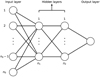Fig. 1 Sketch of NN structure. The network has an input layer with n0 neurons (n0 = 169 for H${}_2^{16}$O and n0 = 171 for H${}_2^{18}$O), two hidden layers with n1 = n2 = 28 nodes, and a single output neuron.

3 Neural network modeling

A NN approach has two main advantages as a functional approximator: first its ability to naturally deal with nonlinear mapping between inputs and outputs, and second its speed in evaluating new examples after the training phase is done.

A NN model consists of nodes (neurons) interconnected through weights (Gardner & Dorling 1998). Each neuron receives an input data that is transformed into an output value according to an activation function. Neurons are grouped in two or more layers and the network is said to be fully connected if every neuron in a layer is linked with every neuron in the successive layer through a weight value: the larger the weight, the larger the contribution given from the corresponding connection to the output of the layer. A graphical representation of a NN is sketched in Fig. 1.

Our first step is to determine the NN structure (Sect. 3.1), then train it to learn how to infer TEV from measured spectra (Sect. 3.2). Once we assess its performance (Sect. 3.3), we apply it to the MIRO data (Sect. 4.1).

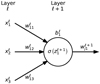Fig. 2 Example of activation function computation for a single neuron. The value of $\sigma (z_i^{\mathcal{l}+1})$ is computed from Eq. (1). The symbols have the meaning specified in Sect. 3.1. In the example shown, nℓ = 3 (number of neurons in layer ℓ), i = 1 (neuron considered in layer ℓ + 1), k = 1, 2, 3 (neuron identifiers for layer ℓ). The value of $\sigma (z_i^{\mathcal{l}+1})$ becomes $x_j^{\mathcal{l}+1}$, which is used to compute the activation function value for neurons j in the successive layer ℓ + 2.

3.1 Network structure

We built twoseparate NN models: one trained for H${}_2^{16}$O spectra and another for H${}_2^{18}$O. We experimented with different NN layouts in order to obtain the simplest structure (i.e., the smallest number of neurons and number of hidden layers), which ensures at least 95% accuracy in estimating the TEV from synthetic spectra, for which we know the correct TEV value by definition. These requirements were satisfied with NN having two hidden layers, each containing 28 neurons. The networks are the same for both spectral transitions.

The activation function σ(z) defines how the output of each neuron is computed from its input (shown in Fig. 2). We adopted the rectified linear unit (ReLU) activation function, defined for neuron i of layer ℓ as $$\begin{array}{l}\sigma \left(z_i^{\mathcal{l}+1}\right)=\max \left\{0,z_i^{\mathcal{l}+1}\right\}\\ z_i^{\mathcal{l}+1}={\sum }_{k=0}^{n_{\mathcal{l}}}{w}_{ik}^{\mathcal{l}}{x}_k^{\mathcal{l}}+b_i^{\mathcal{l}},\end{array}$$

where $w_{ik}^{\mathcal{l}}$ is the weight value from neuron k of layer ℓ to neuron i of the successive layer ℓ + 1; $x_k^{\mathcal{l}}$ is the input value from neuron k of layer ℓ; $b_i^{\mathcal{l}}$ is the bias of neuron i in layer ℓ, that is, a constant value used to offset the result of the activation function; and n_ℓ is the number of neurons in layer ℓ. The quantity $\sigma (z_i^{\mathcal{l}+1})$ becomes the input value $x_i^{\mathcal{l}+1}$ of the considered neuron i of layer ℓ + 1 to be used to compute σ(z_j,ℓ+2) of neuron j in the successive layer ℓ + 2. Compared to other activation functions, the ReLU ensures faster computational time and convergence (Glorot et al. 2011). Initial values for weights $w_{ik}^{\mathcal{l}}$ and biases $b_i^{\mathcal{l}}$, which are changed during the learning process known as backpropagation, were initialized with a normal distribution.

3.2 Training set

The performance of the NN strongly depends on how well the training set represents the real data to which the network will be applied. During the training phase, the network is fed with synthetic (calculated) spectra, for which true TEV is known, and learns by iteratively adjusting the values of weights and biases in order to match its output to the true TEV values. The synthetic spectra database is generated by applying our a 1D spherical symmetric general non-LTE forward model based on the accelerated lambda iteration (ALI), which has previously applied to the MIRO measurements (Marshall et al. 2017; Marschall et al. 2019) and also validated for icy-moon atmospheres (Yamada et al. 2018). The 1D model radial profiles of density follow the Haser distribution,whereas velocity and temperature profiles are parameterized through two variables hyperbolic tangent function and a power law, similarly to Lee et al. (2015) and Zhao et al. (2019). The only additional step is to vary the free variables to create a database that samples the necessary range of densities and velocities as described below.

The training set consists of synthetic nadir spectra for each water isotopolog transition, sampling a variety of input coma conditions using a 1D Haser model. The generated atmospheric inputs have a range of TEV from 0.1 to 1.2 km s⁻¹ and water column density range from 10¹¹ to 10¹⁹ cm⁻² to capture optically thin and thick conditions. The NN is trained with a 80/20 approach: 80% of randomly selected inputs are used for training and the other 20% for validation.

About one-half of the training set (1100 cases) of coma inputs was generated by the 1D Haser model, and the other half is supplemented by scaling sampled atmospheres from direct simulation Monte Carlo (DSMC) simulations of 67P/CG (Liao et al. 2016; Marschall et al. 2016). The Haser model for density profile already depends on assumed velocity and does not provide any guidance on temperature altitude dependence, which in our case is also an empirical modification of a power law similar to Lee et al. (2015) (Eq. (1)–(3)). We find that by including the DSMC samples we get an increase in NN validation accuracy of about 15%. The DSMC model itself is set up for the illumination conditions of the comet on 2015-07-10T01:32:39; subsolar point is −30.48°, such that the southern hemisphere of the cometary surface is illuminated. The boundary conditions for the sublimation of H₂O ice from the nucleus is driven by the insolation at the surface using a simple thermal model from Liao et al. (2016) and Marschall et al. (2016). The H₂O ice is homogeneously distributed all over the nucleus with an effective active fraction of 10%, meaning that 10% of every unit area is active and responds to solar irradiation in the same way. The DSMC simulation domain used extends up to 10 km from the center of the nucleus. To get the gas properties at the spacecraft position, we extracted information from the closest point within the simulation domain and perform a linear interpolation to obtain values for the number density, temperature, and velocity along the LOS as done in Marschall et al. (2019). Two DSMC outputs for production rates of 10²⁶ and 10²⁸ [molec s⁻¹] were used, sampling profiles around the nucleus at 10° steps over the plane spanned by the vector pointing to the Sun and that pointing to the spacecraft position in the comet frame for the chosen date. The extracted profiles from the DSMC provide samples for day, night and terminator conditions. By scaling the density and shifting the velocity of these profiles, we increased their number to about a half of the total number of inputs.

Improvements in the NN performance were expected because the DSMC provides radial profiles of temperature and density near the nucleus that leads to a better agreement in spectral slope of line wings just outside the saturated line cores in the case of the H${}_2^{16}$O transition. Such inputs cannot be generated by the adopted Haser 1D model with the assumed scaling laws of temperature and velocity. In addition, by sampling the different illumination conditions from the model output, as described below, a realistic variability of inputs is obtained and provides a further improvement.

The benefit of including the DSMC inputs, it should be made clear, does not rest on the expectation that the 3D model provides accurate absolute values of the inputs. First, a physical inconsistency is guaranteed by shifting the extracted velocity profiles and scaling the water densities. In this work this fact has no effect on the NN performance, the output accuracy, or the latter interpretation. Density and temperature profiles do not influence the center frequency Doppler shift, which is the parameter of interest. Second, the line center frequency of the water transitions, already for moderately optically thick conditions, forms well above the actual computational domain of the DSMC (~10 km). Therefore, the benefit lies in the fact that by sampling DSMC outputs (including modifications we described) we obtain a set of synthetic line shapes that the 1D Haser parametrization cannot capture. It is in principle possible to create a more complex 1D parametrizations that would be able to provide better and more complete approximations observed in the MIRO lines. At the same time, we would expect that it is possible to create a comprehensive training database using only DSMC samples, if more runs were available. Nevertheless, the hybrid approach we describe gave us a perfect trade-off managing computational speed, flexibility in range, sampling density of inputs, and reducing implementation complexity. In the case of future work, when a NN is tasked with a more difficult problem, such as entire vertical profile retrievals, the hybrid approach may have to be re-evaluated.

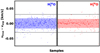Fig. 3 Neural network TEV predictions for H${}_2^{16}$O (blue, left) and H${}_2^{18}$O (red, right) validation data. The x-axis represents an arbitrary index number of a data point. The scattered points represent the difference between the known terminal velocity (vtrue) of each synthetic spectra and the velocity predicted by the network (vexp). The horizontal black lines indicate ±0.03 km s−1 : the fraction of points enclosed in this region is 95% for H${}_2^{16}$O and 96% for H${}_2^{18}$O. The shaded colored region indicate a 1σ error on the predictions: 0.017 km s−1 for H${}_2^{16}$O and 0.015 km s−1 for H${}_2^{18}$O.

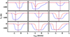Fig. 4 Nine randomly selected spectra from a validation set for H${}_2^{16}$O (blue) and H${}_2^{18}$O (red). The blue and red vertical lines indicate the mean retrieved TEV for H${}_2^{16}$O and H${}_2^{18}$O, respectively. The shaded regions around these lines represent a 1σ error (see description in Sect. 3.3). The black vertical line indicates the true TEV corresponding to the synthetic atmosphere used to generate each pair of H${}_2^{16}$O/H${}_2^{18}$O absorption features.

3.3 Validation

The validation step allows us to perform a statistical analysis of a trained NN outputs with the true values, assessing the performance of the network. As noted above, 20% of the entire training data are set aside for validation. In the validation phase, as well as in subsequent application to real measured MIRO spectra, we do not include absorption lines whose line area is smaller than 4.5 K km s⁻¹, which cannot be reliably distinguished from noise.

Figure 3 shows statistical plots of the goodness of predictions made by the NNs for H${}_2^{16}$O and H${}_2^{18}$O. Criteria for correct predictions is set within ±0.03 km s⁻¹ with respect to the true TEV. The 30 m s⁻¹ corresponds roughly to the uncertainty in the MIRO calibration of the frequency grid (i.e., the width of a single spectral channel; 25 m s⁻¹). The NNs used in this work over several runs perform with an accuracy of 95% for H${}_2^{16}$O and 96% for H${}_2^{18}$O.

Figure 4 further illustrates the NN performance, showing nine randomly selected validation spectra, the true TEV, and the predicted TEV. The uncertainty in NN outputs is estimated by performing 50 complete runs with fixed training and validation dataset. The estimated 1σ is a measure of the uncertainty inherent in the NN itself due to its nonlinear nature and design (e.g., shuffling the order of inputs in which they are presented to the NN during training, random initialization of weights and biases).

As shown in Fig. 4, the trained NN is able to very accurately perform the inverse mapping from spectra to TEV. In fact it is visually not possible to distinguish the vertical lines as they overlap each other, thereby confirming the excellent agreement between the H${}_2^{16}$O and H${}_2^{18}$O TEV estimates and the true value. We want to emphasize that even in cases of completely saturated line cores prevalent for H${}_2^{16}$O lines for high water column densities, the NN is able to extract TEV with great accuracy and statistical stability. We find no inherent biases in the trained NN for predicting TEV from the calculated H${}_2^{16}$O and H${}_2^{18}$O spectra. In other words, TEVs predicted from either spectral line are always within the uncertainty estimate to be inherent in the NN itself (1σ error), which is always smaller than the single channel uncertainty in velocity calibration of MIRO spectra.

4 Results and discussion

4.1 Application to measurements

As in the validation phase, we estimate TEVs from the measured MIRO data by averaging 50 runs of the NN, each automatically differing in the selection of training profiles and weights initialization. We opt for this approach to capture and quantify the uncertainty in TEV estimation due to NN setup itself. The 1σ error is computed as the standard deviation of the 50 runs output. Additionally, we exclude from the prediction step any spectra with a line area smaller than 4.5 K km s⁻¹, which cannot be reliably distinguished from random noise. This mostly affects the H${}_2^{18}$O spectra for conditions of low H₂O column density that occur for early and late mission phases, and for night side observations. All estimates of TEVs and their uncertainties are made available online². Below, we present the main results of correlations and time evolution analysis of the retrieved TEVs.

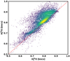Fig. 5 Joint density distribution between TEVs inferred from H${}_2^{16}$O and H${}_2^{18}$O spectra measured by the MIRO instrument. In this summary plot, all data (from August 2014 until July 2016) are shown excluding cases of low S/N based on the line area. Although there is a strong correlation it is apparent that the H${}_2^{18}$O spectra yield higher velocity for a considerable fraction of the dataset (see text for details).

4.2 TEVs and line area variations

We first investigated whether there are relationships between the H${}_2^{16}$O and H${}_2^{18}$O estimated TEVs. The correlation between the H${}_2^{16}$O and H${}_2^{18}$O TEV estimates is shown in Fig. 5 plotted as a 2D joint density distribution. The color bar in the plot is qualitative with bright (yellow) color indicating higher frequency of occurrence.

We can see that the cloud of points aligns as expected for a positive correlation between the two TEV estimates. However, it is also evident that TEVs from H${}_2^{18}$O spectra show a considerable number of data points with larger absolute values, especially when TEV(H${}_2^{16}$O) is above 650 m s⁻¹. The estimated uncertainty on the individual data points can be considered small, ranging from 5 to 30 m s⁻¹ in most cases. There are a few statistical outliers with larger uncertainty, mainly in the case of the weaker H${}_2^{18}$O isotope withlower signal-to-noise ratio (S/N). In addition, we notice that the range of estimated TEVs is between 0.5 and 0.9 km s⁻¹, as shown in Fig. 5. As the low TEV values (<500–600 m s⁻¹) generally occur for conditions of lower number densities (e.g., shadowed regions and/or large heliocentric distances), the sampling is worse by the weaker H${}_2^{18}$O measurements than for main isotopolog H${}_2^{16}$O. This is also apparent in subsequent figures.

We also analyzed whether a relationship exists between the extracted TEVs from each transition and their corresponding spectrum line area, but we found no strong correlations. Part of the reason for the weak correlation stems from the high opacity of the H${}_2^{16}$O line for most of the observational period. Therefore, the growth of line area is nonlinear with increasing production rate. However, despite the lower opacity of the H${}_2^{18}$O transition, we also did not find a strong correlation. Therefore, from a global dataset perspective the TEVs are not connected to the line area by a simple linear relationship.

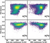Fig. 6 Joint density distribution between derived TEVs and MIRO sub- and millimeter continuum antenna temperatures, The labels in each panel indicate to which isotopolog of water the TEV belongs. The color bar is qualitative, where bright colors indicate a higher frequency of occurrence (yellow) and dark blue represents low frequency of occurrence.

4.3 Continuum temperature variation

The MIRO instrument also provides direct measurements of continuum temperatures in two channels. Full details on the relation between theMIRO antenna and the physical temperature of a target is available in the user manual (Frerking et al. 2018).³ Since we explore only trends and correlations we do not convert the continuum antenna temperatures to the physical temperature. Center frequencies of the continuum receivers for submillimeter (sub-MM) and millimeter (MM) wavelengths are 552 (~0.53 mm) and 188 GHz (~1.6 mm), respectively (Gulkis et al. 2007). Since the instrument operated mostly in dual mode, we have simultaneous spectra and continuum measurements, which are certainly connected by physical relationship. For instance, the (sub)surface temperatureat which a molecule undergoes its last collision before it escapes from the surface determines its initial velocity.

Figure 6 shows correlation plots of TEV with both sub-MM and MM continuum measurements for the two transitions. The color bar represents a density function, with brighter colors indicating a higher frequency of occurrence. In this overall picture we do not find a notable relationship with the sub-MM or MM continuum temperature for either of the water transitions. The low TEVs (H${}_2^{16}$O) (<0.6 km s⁻¹) tend to occur predominantly when sub-MM antenna temperatures are below 175 K; however, these would correspond to times of earlier phases of the mission. Similarly, we can see that for TEVs (H${}_2^{18}$O) the data form a point cloud without any strong correlation. To highlight this point we present more detailed analysis of density plots split into several time segments in Appendix B. Nevertheless, even then it is difficult to extract a general conclusion from these plots. This may be not surprising since the different illumination and observation conditions are not separated asthey evolve with time. A more elaborate analysis may be required to extract more information on the dependence of TEV and continuum temperatures.

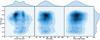Fig. 7 Joint probability/density distributions for H${}_2^{16}$O TEV vs. effective LT (left), SZA (middle), and effective VA (right). The 1D probability distributions of each axis are also shown. See Sect. 4.4 for detailed description and interpretation.

4.4 Solar zenith angle correlations

Next, we consider the TEV variation with the effective SZA, LT and the VA⁴. The effective SZAs, LTs, and VAs represent the mean values of the respective variables determined as an average for all facets that lie within two times the HPBW of MIRO’s beam projected on the surface using the 125k SHAP7 shape model (Preusker et al. 2017). The projected size of MIRO’s beam varies with time as the spacecraft distance changes during the mission phases. Despite the complexity of considering effective mean variables, it is natural to look for correlations from a point of view of the entire dataset, to spot whether there are prevalent statistical relations among the variables. For example, it would be of interest to find an analog of spatial and temporal variations of gas TEV with SZA, as has been established for dust jets (Lai et al. 2019).

Figure 7 summarizes the TEV(H${}_2^{16}$O) variation with LT (left), SZA (middle), and VA (right). The blue nuances correspond to the joint probability distribution between the variables: the darker the color, the higher the joint probability. The 1D distribution over a given parameter from the entire dataset is shown on top of each panel (LT, SZA, VA) and for TEV on the vertical axis of the rightmost plot.

The TEV 1D probability distribution curve reflects changes in the physical conditions of the coma (e.g., heliocentric distance) and the observation geometry. It is clearly not Gaussian shaped but has a general resemblance of a bimodal distribution. As already noted, the low TEV values would predominantly correspond to the early and late mission phases (months of 2014 and 2016), while the high velocities occurred in 2015, that is, near perihelion. In the 1D distribution over the LT we clearly get a bimodal structure with long tails on either side. This is due to a combinationof nadir geometry (of this dataset) and a preference to operate the spacecraft close to the terminator orbit whenever possible. This is also reflected in the effective SZA probability distribution (middle panel), which peaks near 75°. The VA distribution has a single, but broad, peak around 50°.

The shape of the joint probability is not symmetric around noon (LT 12) and shows a slight tendency for higher TEV values before noon, but the lower values (<0.5 km s⁻¹) have non-negligible probability shifted toward later afternoon LT. The TEVs in the range 0.7 ± 0.05 km s⁻¹ seem to occur with the broadest range of LT (from 5 to 20 h). Similarly, this range of TEVs shows a wide non-negligible probability range over SZA and VA distribution. The largest H${}_2^{16}$O TEV values around 0.9 km s⁻¹ are shown with narrower, flat probability distribution over range of values of LT (11–15 h) or SZA (30–110°).

The most frequent TEV over the entire dataset is about 0.8 ± 0.05 km s⁻¹, occurring mostly at around 9–10 h in the morning or 15 h afternoon. The TEV and VA joint probabilities appear more uniform, dominated by the single peak in the VA distribution. Nonetheless, TEV values above 0.7 km s⁻¹ can also occur even at VAs larger than 70°, unlike low TEV values, which tend to cluster between 20 and 40°.

The TEV(H${}_2^{18}$O) joint probability distributions with LT, SZA, and VA are shown in Fig. 8. The panels, axis description, and color scale are the same as in Fig. 7. We note that minor isotopolog line strength is about 500 times weaker than the main line strength. Therefore, most of the TEV values in the early and late mission phases (2014 and 2016) are not sampled, giving the TEV 1D distribution a much narrower form, although still appearing multimodal. The missing data from early and later phases also present modified 1D distributions of LT, SZA, and VA; however, in a broad sense they retain the same characteristics as those for H${}_2^{16}$O.

We note that H${}_2^{18}$O TEV distribution between 0.8–0.9 km s⁻¹ displays a double-peak structure at ~9 and ~15 h LT. We can also see non-negligible occurrence frequency of 0.9 km s⁻¹ velocities for LT around 5–7 h. On the other hand, TEVs of around 0.7 km s⁻¹ shows a flatter distribution over a narrower range of LT (9–16 h). Compared to H${}_2^{16}$O data shown in Fig. 7, the joint distributions appear rather symmetric around the region of maximum probabilities for LT, SZA and VA parameters. This is because the H${}_2^{18}$O dataset does not sample the early and late mission phases properly owing to generally lower water vapor production rates during these times.

Fig. 8 Same as in Fig. 7 but for H${}_2^{18}$O TEV. The white space below 0.35 km s−1 indicates no data.

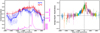Fig. 9 Left: time evolution of estimated TEVs from the two water transitions; the blue points indicate H${}_2^{16}$O and the red points indicate H${}_2^{18}$O; each point represents a daily mean and the error bars indicate the corresponding standard deviation. The solid red and blue lines denote 30 d running averages. The spacecraft cometo-centric distance is shown in the same panel as the magenta line. Right: daily averaged difference and its standard deviation shown as vertical lines for collocated data points as a function of time. The point clouds of different colors correspond to a different month (August 13, 2015 was the perihelion passage). There is a definite TEV dependence on the heliocentric distance, where the velocities obtained from H${}_2^{18}$O transitions tend to be larger starting from around May 2015, peaking in August–September 2015, and decreasing again afterward. The maximum differences are on the order of 0.15–0.2 km s−1. See Sect. 4.5 for discussion.

4.5 Heliocentric evolution of TEV

Figure 9 shows the time evolution of TEVs as a function of days from perihelion. The left panel indicates daily mean values for H${}_2^{16}$O (blue) and H${}_2^{18}$O (red) along with corresponding standard deviations. The weaker isotope transition is not detectable for low production rates in the early and late mission phases as pointed out previously. The range of TEVs is also smaller for the minor isotope since measurements of low production rate conditions (night/shadow) cannot be made with reliable sensitivity. Importantly, we can clearly observe the aforementioned difference in TEVs magnitude from the two isotopic lines. The right panel in Fig. 9 presents daily averages of the H${}_2^{16}$O and H${}_2^{18}$O TEV difference with their standard deviation shown as a thin vertical line. The differences are possible only when we have the same data point in time for both measurements, which explains the gaps in the data for the early and late mission phases. The data point clusters of the same color represent a particular month of the year (with perihelion passage occurring in August 2015).

The observed differences in TEVs is the most puzzling aspect of the two datasets. It is unambiguous that the differences grow larger approaching the perihelion. There, these differences reach about 0.15–0.2 kms⁻¹, which is more than five spectral channels of MIRO. The MIRO frequency calibration uncertainty is better than one channel, which indicates that these deviations are significant. For another view of the TEV differences, we plot nine randomly selected MIRO measured spectra in Fig. 10, one for each month in 2015 as shown in labels. The shallow absorption line (orange) is for the H${}_2^{18}$O and the deeper and the wider spectral line is for the simultaneously measured H${}_2^{16}$O isotopolog. The vertical lines in each panel correspond to the estimated TEVs by the NN.

Even for individually randomly selected spectra, the differences are easily perceived as the separation between thevertical lines is growing when approaching August–September 2015. We scrutinized the NN inversion for potential biases and can confidently rule this out as a source of the discrepancy. In particular, H${}_2^{18}$O TEV are properly identified as the vertical line intersects the minimum of the corresponding spectral line. The H${}_2^{16}$O spectra withits fully saturated line core, makes the visual identification of correct Doppler shift more difficult. However, as shown in our simulations (see Fig. 3 and also Fig. A.1 with contribution functions), the correct Doppler offset qualitatively falls in the middle of the saturated (flat) portion of the line. The NN also accurately recovers theTEVs for cases in between optically thin and complete line core saturation. As shown in the NN validation (Sect. 3.3), the NN is able to obtain accurate (i.e., within one channel width) TEV from the H${}_2^{16}$O spectra independent of optical thickness or line shape complexity.

Neither frequency calibration nor NN inversion for TEV seem to be the reason for the observed differences. Hence, we need to consider the TEV differences estimated from the two different spectral lines arising through a physical mechanism. The heavier isotopolog (H${}_2^{18}$O) spectra yields a faster expansion velocity. Also, because of its smaller opacity, these spectra sample regions at around 10–20 km from the nucleus surface even for large water column density (see Appendix A). The line center of H${}_2^{16}$O spectra typically forms at higher altitudes, even above 100 km altitude for larger production rates. Therefore, if the H₂O gas velocity begins to decrease for some reason above around 10–20 km, the TEV difference would be manifested directly in MIRO measurements of the radiance of the main water isotopolog. The cometo-centric distance of Rosetta varies with time and happens to reach consistently above 150 km altitude around and through the perihelion passage. Therefore, owing to the higher water production rates the MIRO measurement of the optically thick H${}_2^{16}$O are formed at higher altitudes (see Appendix A) than the optically weak H${}_2^{18}$O. Hence, if there is an extended source of water gas, this could very well fit the observed behavior of TEV. The extended sources and its effects (including velocity radial profiles) were already modeled to explain the observed slow decay of water rotational temperatures and densities for the comet 73P/Schwassmann-Wachmann 3B in Fougere et al. (2012).

Therefore, our first hypothesis builds on the extended source of gas occurring around the perihelion passage. As the comet approaches perihelion, the gas production rate is increased such that icy aggregates are lifted and start outgassing as they become embedded in the faster outflow (Keller et al. 2017). The velocity of released gas, while depending on the temperature of these larger aggregates, would be lower compared to the velocity of gas that has accelerated from the comet surface up to a given height. In addition, if we suppose they are not oriented on average such that the released gas in the direction of the bulk flow, it would also result in a slower average outflow velocity within the MIRO sampled volume. This hypothesis would also suggest that kinetic temperature of the gas should be higher, which has been already noted in several MIRO observations in May 2015 (Marschall et al. 2019).

A second plausible hypothesis to explain the implied deceleration of natural gas above the line center formation of H${}_2^{18}$O line is the ion-netural gas drag at the boundary of diamagnetic cavity (Gombosi 2015). The diamagnetic cavity region in coma of the comet is manifested when the incoming (solar) plasma is strongly decelerated as to become stagnant at some altitude range with an associated build-up of a magnetic barrier around it. This typically happens in the close nucleus region (approximately below 100 km depending on Q[H₂O]) because the ion-neutral collisions tend to slow the in-flowing plasma. There are already reliable hybrid model simulations of this effects in the context of 67P/CG in Koenders et al. (2015). The observational evidence for the presence of the diamagnetic cavity, or a structure similar to it, in the coma of 67P/CG is provided by the Rosetta Plasma Consortium suite of instruments monitoring the proton and alpha particle bulk properties as a function of time (Behar et al. 2017). It was found that from around mid-April 2015 until mid-December 2015 there is complete lack of solar wind particles at the location of Rosetta spacecraft because these are deflected by the magnetic barrier associated with the diamagnetic cavity. Nevertheless, there is still little knowledge about the coupling effects of neutral gas deceleration by the stagnant plasma, especially the magnitude, altitude extend of this mechanism, and whether the kinetic temperature increase would also be affected.

A global 3D DSMC hybrid models could be used to weigh in as to which scenario is a better explanation of the observed TEV differences obtained from the two isotopolog water transitions. However, a model capable of handling the coupling of gas-dust and ion-gas to obtain self-consistently the neutral gas velocity and temperature is not yet available to our knowledge. The desired model domain for this problem extends at least several 100 km with adaptive grid to allow at least 2 km resolution below 20–30 km. It is desirable to perform such simulations in the future to disentangle the TEV evolution of measurements from MIRO.

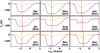Fig. 10 Randomly selected cases of measured spectra and their predicted TEV for each month (as labeled) in 2015. Purple indicates H${}_2^{16}$O spectra and its TEV estimate; orange indicates likewise for H${}_2^{18}$O. The vertical lines indicate the predicted TEV, with the shaded region representing the estimated 1σ error (see text for details).

5 Conclusions

We implemented and analyzed the performance of a NN for retrieving gas terminal velocity from (H${}_2^{16}$O and H${}_2^{18}$O) rotational transition measured by the MIRO instrument in nadir geometry. The high spectral resolution of MIRO allows us to infer this information from the Doppler shift of the two spectral lines independently. Although the Doppler effect is measured along the MIRO beam LOS, it is expected that the TEVs represent an actual radial outflow values as long as the line center weighting function peak aroundabout 10 km altitude or higher (Marschall et al. 2016). As demonstrated in Sect. 3.3 the NN can be trained on pre-calculated examples to reach a very high accuracy (95%) extracting TEV even from saturated line cores in the H${}_2^{16}$O absorption line. Importantly, the NN method for TEV retrieval is free from systematic biases. We stress that characteristics of the training set, such as the size and coverage of the expected domain, plays a key role in the NN performance. In our case, we found that using even modest samples from 3D DSMC simulations had substantial effects (~15% improved accuracy), which is mainly due to more physical vertical profiles of kinetic temperature and velocity than achievable with power law approximations typically used in 1D coma models.

We performed 50 independent iterations of training and TEV estimations for each measured spectra to estimate uncertainties originating from the NN method itself. The same approach was also used in the validation phase for the NN, for which we know the true values of velocities. We find that TEV uncertainties from the NN itself are smaller than one channel (30 m s⁻¹) and are not systematically biased. The calibration uncertainties of MIRO frequency are also smaller than a single channel. The chirp transform spectrometer of MIRO has an absolute frequency stability of 4 KHz and is unlikely to get frequency inaccuracies of more than 10 kHz (0.005 km s⁻¹) from the USO even in the worse case assumptions. The frequency stability of the CTS versus temperatures are documented⁵, and are also smaller than the channel width (44 kHz). Therefore, the derived TEV differences from the two isotopic lines of more than (0.15 km s⁻¹) are highly unlikely a consequence of the NN method or the measurement uncertainties themselves.

We apply the NN to all suitable MIRO spectra (see Sect. 2) for both water transitions, based on a minimum line area criterion. We retrieve about 28 000 TEVs from H${}_2^{16}$O and about 12 000 from H${}_2^{18}$O spectra; the tables are available online⁶.

The key points from our global TEV dataset analysis can be summarized as follows:

• From the perspective of the aggregate dataset, we found no correlation between TEV and MM or sub-MM continuum temperatures measured by MIRO that would suggest a direct physical link with the surface. However, a more detailed study of this relationship is warranted in the future that would, for instance, focus predominantly on the data points taken under the same illumination and observation conditions.

• Joint probability plots of TEV and LT reveal that the highest velocities are almost equally likely to occur in the range between 9–15 h LT. Nevertheless, for H${}_2^{16}$O, the most frequent TEV range of 0.8 ± 0.05 km s⁻¹ has a bimodal distribution in the LT range of 9 and 15 h. This distribution is asymmetric and large velocities in excess of 0.7 km s⁻¹ may appear over a broad range of LTs (5–20 h). The TEVs estimated from H${}_2^{18}$O spectra follow similar bimodal distribution characteristics of the main isotope. We add a word of caution to this local correlation analysis, since it has been shown that a surface area intercepted by MIRO beam may not be responsible for the bulk of molecules in the upper regions of coma where the spectral lines form. This statement has a general validity. These correlation-based conclusions should be viewed in a statistical sense and may not apply to specific data points over a particular time. More elaborate analyses, considering similar illumination conditions over a particular region, should be used to draw more solid and definite conclusions.

• The TEVs from H${}_2^{18}$O do not always agree with those from H${}_2^{16}$O transition. There is a time dependence to these differences, starting at nearly perfect agreement from August 2014 until beginning of 2015, but growing in May 2015 onward and peaking in August–September 2015 (~150 m s⁻¹). Subsequently, the differences decrease with time again. We ruled out the possibility that this discrepancy is due to either the NN method itself or frequency biases in MIRO calibration.

• Understanding that the MIRO measured H${}_2^{16}$O spectral line core forms at higher altitudes than the H${}_2^{18}$O (Appendix A), we considered two plausible mechanisms that could potentially explain the difference in their TEVs. First, we discussed an extended source of water molecules in the coma as the comet approaches perihelion, supplying slower and warmer gas above 20–50 km altitude. This effect was studied and proposed to explain measured decay profiles in rotational temperatures for a comet 73P-B/Schwassmann–Wachmann 3B Fougere et al. (2012). A second hypothesis we discussed suggests that an ion drag might be responsible for the deceleration of the neutral gas in the region around the diamagnetic cavity, which occurs in the coma for higher production rates. This type of structure was observed in 67P/CG (Koenders et al. 2015; Behar et al. 2017). However, the magnitude of this effect and whether it would also provide an increase in neutral gas kinetic temperatures, as was shown to occur in the upper coma regions in Marschall et al. (2019), remains to be modeled.

• In relation to the previous point, we also observed that the maximum TEV values from the two transitions do not necessarily coincide in time or space, especially for near-perihelion data. This might be expected if the information on the TEV from the Doppler shift of each isotopolog line comes from very different altitudes as discussed in the text. We hope that future model studies capable of combining dust-gas and gas-ion coupling may bring new knowledge about the source of these differences.

• The NN approach for TEV retrieval could be also applied to other measurements of MIRO (H${}_2^{17}$O, CO, CH₃OH, or NH₃). However, because of the low optical thickness in these spectral lines they also form in the lower altitude in the coma and the estimated TEV should follow closely the estimated TEV from H${}_2^{18}$O. However, it is still desirable to obtain TEVs from other molecular transitions whether or not they agree with our prediction, perhaps identifying conditions where the TEVs imply only a weak coupling with the water gas. This could shed light on other aspects of cometary activity and gas release from the nucleus.

As a general remark we find the NN method surprisingly effective in handling the problem of estimating TEVs from the MIRO spectra, especially in the case of saturated lines. We emphasize the need to carefully consider and build the training datasets covering theexpected domain to which the NN will be applied. The NN is a promising tool in combination with the 3D forward models in many domains of science application, for instance to approximate radiative transfer calculations, retrieve parameters from nonlinear relationships to measurements, or simply provide a quick first estimate to constrain the initial conditions of more computationally intensive retrievals.

Acknowledgements

Rosetta is an European Space Agency (ESA) mission with contributions from its member states and NASA. We acknowledge the entire ESA Rosetta team and thank them for their contribution, without which this work could not have been done. This extends also to the ESA planetary science archive and the MIRO PI: M. Hofstadter (NASA/JPL, Pasadena, USA). L.R. was partially funded from the DFG-392267849.

Appendix A H${}_2^{16}$O and H${}_2^{18}$O contribution functions

We present sample contribution functions for H${}_2^{16}$O (Fig. A.1) and H${}_2^{18}$O (Fig. A.2) transitions that are routinely measured by the MIRO instrument and used for TEV estimation in this work. At each frequency (velocity) these functions provide visual information on the peakaltitude and vertical extent of altitude region where the measured radiance at a particular velocity is formed. These simulation are done for optically thick conditions, with water column density set to 5 × 10¹⁶ cm⁻². Therefore, the shown examples are representative of near-perihelion daytime production rates, for which we observe the largest differences between TEV from the two spectra.

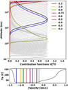Fig. A.1 Top: contribution functions for H${}_2^{16}$O transition at 557 GHz normalized to the maximum value to clearly indicate the peak altitude at each velocity/frequency point. These were calculated for an optically thick case of water column density 5 × 1016 cm−2. The terminal velocity in the input atmosphere for these calculations is set to −0.75 km s−1 and is reached at about 3.5 km from surface. The other color lines correspond to different velocity offsets for comparison, and correspond to the vertical lines in the bottom panel. The rest of the velocities are shown in gray lines. Bottom: synthetic spectra line are shown for reference. The vertical lines depict locations in velocity space corresponding to the contributionfunctions shown in the top panel.

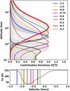Fig. A.2 Same is in Fig. A.1, but for the H${}_2^{18}$O transition at 548 GHz. The telluric ratio is assumed between the isotopologs. The outgoing radiance comes from deeper levels in the coma compared to the H${}_2^{16}$O.

Appendix B Evolution of TEV correlations with continuum temperatures

Supporting figures to the discussions in Sect. 4.3 are provided in this appendix. Figures B.1 and B.2 also contain TEV versus continuum temperature density plots with the dataset split into several time segments. The color bar is qualitative, where brighter colors (yellow) denote higher frequency of occurrence. The time segments are indicated in the label and apply to each row. They were chosen to get a large enough statistical sample but still provide meaningful time evolution, especially for the near-perihelion passage.

From the time evolution point of view in Fig. B.1 we observe the shape of the distribution is changing, from what can be considered a compact shape in August–December 2014 to a progressively more elongated correlation covering larger range of continuum temperatures around July–September 2015, and then again becoming more compact again (smaller range of sub-MM temperatures) until April–July 2016. In the last time segment the weaker water isotopolog does not yield enough data to compare it meaningfully with the H${}_2^{16}$O plot since the production rates were small and the spacecraft was close to the nucleus. From these plots we also conclude that there is no obvious correlation between the two quantities during any of the time periods. However, interpretation of these density plots is a difficult task because of the many time varying parameters that are effectively still convolved together in the dataset we consider. A more sophisticated study is needed which would only compare data for the same illumination conditions, space-craft distance, and so on. Similarly, we gain only qualitative picture of the general behavior from the Fig. B.2.

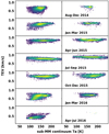Fig. B.1 Density plot of derived TEVs vs. sub-MM continuum temperatures as a function of time as shown in the labels. Left column: corresponds to TEVs using the H${}_2^{16}$O measurements. Right column: TEVs from H${}_2^{18}$O.

Fig. B.2 Same as in Fig. B.1, but for continua temperatures from the MM channel.

References

All Figures

	Fig. 1 Sketch of NN structure. The network has an input layer with n0 neurons (n0 = 169 for H${}_2^{16}$O and n0 = 171 for H${}_2^{18}$O), two hidden layers with n1 = n2 = 28 nodes, and a single output neuron.
In the text

Fig. 2 Example of activation function computation for a single neuron. The value of $\sigma (z_i^{\mathcal{l}+1})$ is computed from Eq. (1). The symbols have the meaning specified in Sect. 3.1. In the example shown, nℓ = 3 (number of neurons in layer ℓ), i = 1 (neuron considered in layer ℓ + 1), k = 1, 2, 3 (neuron identifiers for layer ℓ). The value of $\sigma (z_i^{\mathcal{l}+1})$ becomes $x_j^{\mathcal{l}+1}$, which is used to compute the activation function value for neurons j in the successive layer ℓ + 2.

In the text

Fig. 3 Neural network TEV predictions for H${}_2^{16}$O (blue, left) and H${}_2^{18}$O (red, right) validation data. The x-axis represents an arbitrary index number of a data point. The scattered points represent the difference between the known terminal velocity (vtrue) of each synthetic spectra and the velocity predicted by the network (vexp). The horizontal black lines indicate ±0.03 km s−1 : the fraction of points enclosed in this region is 95% for H${}_2^{16}$O and 96% for H${}_2^{18}$O. The shaded colored region indicate a 1σ error on the predictions: 0.017 km s−1 for H${}_2^{16}$O and 0.015 km s−1 for H${}_2^{18}$O.

In the text

Fig. 4 Nine randomly selected spectra from a validation set for H${}_2^{16}$O (blue) and H${}_2^{18}$O (red). The blue and red vertical lines indicate the mean retrieved TEV for H${}_2^{16}$O and H${}_2^{18}$O, respectively. The shaded regions around these lines represent a 1σ error (see description in Sect. 3.3). The black vertical line indicates the true TEV corresponding to the synthetic atmosphere used to generate each pair of H${}_2^{16}$O/H${}_2^{18}$O absorption features.

In the text

Fig. 5 Joint density distribution between TEVs inferred from H${}_2^{16}$O and H${}_2^{18}$O spectra measured by the MIRO instrument. In this summary plot, all data (from August 2014 until July 2016) are shown excluding cases of low S/N based on the line area. Although there is a strong correlation it is apparent that the H${}_2^{18}$O spectra yield higher velocity for a considerable fraction of the dataset (see text for details).

In the text

	Fig. 6 Joint density distribution between derived TEVs and MIRO sub- and millimeter continuum antenna temperatures, The labels in each panel indicate to which isotopolog of water the TEV belongs. The color bar is qualitative, where bright colors indicate a higher frequency of occurrence (yellow) and dark blue represents low frequency of occurrence.
In the text

	Fig. 7 Joint probability/density distributions for H${}_2^{16}$O TEV vs. effective LT (left), SZA (middle), and effective VA (right). The 1D probability distributions of each axis are also shown. See Sect. 4.4 for detailed description and interpretation.
In the text

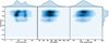	Fig. 8 Same as in Fig. 7 but for H${}_2^{18}$O TEV. The white space below 0.35 km s−1 indicates no data.
In the text

Fig. 9 Left: time evolution of estimated TEVs from the two water transitions; the blue points indicate H${}_2^{16}$O and the red points indicate H${}_2^{18}$O; each point represents a daily mean and the error bars indicate the corresponding standard deviation. The solid red and blue lines denote 30 d running averages. The spacecraft cometo-centric distance is shown in the same panel as the magenta line. Right: daily averaged difference and its standard deviation shown as vertical lines for collocated data points as a function of time. The point clouds of different colors correspond to a different month (August 13, 2015 was the perihelion passage). There is a definite TEV dependence on the heliocentric distance, where the velocities obtained from H${}_2^{18}$O transitions tend to be larger starting from around May 2015, peaking in August–September 2015, and decreasing again afterward. The maximum differences are on the order of 0.15–0.2 km s−1. See Sect. 4.5 for discussion.

In the text

	Fig. 10 Randomly selected cases of measured spectra and their predicted TEV for each month (as labeled) in 2015. Purple indicates H${}_2^{16}$O spectra and its TEV estimate; orange indicates likewise for H${}_2^{18}$O. The vertical lines indicate the predicted TEV, with the shaded region representing the estimated 1σ error (see text for details).
In the text

Fig. A.1 Top: contribution functions for H${}_2^{16}$O transition at 557 GHz normalized to the maximum value to clearly indicate the peak altitude at each velocity/frequency point. These were calculated for an optically thick case of water column density 5 × 1016 cm−2. The terminal velocity in the input atmosphere for these calculations is set to −0.75 km s−1 and is reached at about 3.5 km from surface. The other color lines correspond to different velocity offsets for comparison, and correspond to the vertical lines in the bottom panel. The rest of the velocities are shown in gray lines. Bottom: synthetic spectra line are shown for reference. The vertical lines depict locations in velocity space corresponding to the contributionfunctions shown in the top panel.

In the text

	Fig. A.2 Same is in Fig. A.1, but for the H${}_2^{18}$O transition at 548 GHz. The telluric ratio is assumed between the isotopologs. The outgoing radiance comes from deeper levels in the coma compared to the H${}_2^{16}$O.
In the text

	Fig. B.1 Density plot of derived TEVs vs. sub-MM continuum temperatures as a function of time as shown in the labels. Left column: corresponds to TEVs using the H${}_2^{16}$O measurements. Right column: TEVs from H${}_2^{18}$O.
In the text

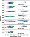	Fig. B.2 Same as in Fig. B.1, but for continua temperatures from the MM channel.
In the text

References

- Acton, C. H. 1996, Planet. Space Sci., 44, 65 [NASA ADS] [CrossRef] [Google Scholar]
- Behar, E., Nilsson, H., Alho, M., Goetz, C., & Tsurutani, B. 2017, MNRAS, 469, S396 [CrossRef] [Google Scholar]
- Biver, N., Hofstadter, M., Gulkis, S., et al. 2015, A&A, 583, A3 [NASA ADS] [CrossRef] [EDP Sciences] [Google Scholar]
- Biver, N., Bockelée-Morvan, D., Hofstadter, M., et al. 2019, A&A, 630, A19 [NASA ADS] [CrossRef] [EDP Sciences] [Google Scholar]
- Combi, M. R., Harris, W. M., & Smyth, W. H. 2004, Comets II, eds. M. C. Festou, H. U. Keller, & H. A. Weaver (Tucson: University of Arizona Press), 523 [Google Scholar]
- Davidsson, B. J. R. 2008, Space Sci. Rev., 138, 207 [Google Scholar]
- Davidsson, B. J. R., Gulkis, S., Alexander, C., et al. 2010, Icarus, 210, 455 [NASA ADS] [CrossRef] [Google Scholar]
- Fougere, N., Combi, M., Tenishev, V., et al. 2012, Icarus, 221, 174 [NASA ADS] [CrossRef] [Google Scholar]
- Frerking, M., Gulkis, S., Hofstadter, M., et al. 2018, MIRO Experiment User Manual, Issue 7.0, RO-MIR-PR-0030 [Google Scholar]
- Gardner, M., & Dorling, S. 1998, Atmos. Env., 32, 2627 [Google Scholar]
- Glorot, X., Bordes, A., & Bengio, Y. 2011, J. Mach. Learn. Res., 15, 315 [Google Scholar]
- Gombosi, T. I. 2015, Physics of Cometary Magnetospheres (USA: American Geophysical Union), 169 [Google Scholar]
- Gulkis, S., Frerking, M., Crovisier, J., et al. 2007, Space Sci. Rev., 128, 561 [NASA ADS] [CrossRef] [Google Scholar]
- Gulkis, S., Allen, M., von Allmen, P., et al. 2015, Science, 347, 0709 [Google Scholar]
- Keller, H. U., Mottola, S., Hviid, S. F., et al. 2017, MNRAS, 469, S357 [CrossRef] [Google Scholar]
- Koenders, C., Glassmeier, K.-H., Richter, I., Ranocha, H., & Motschmann, U. 2015, Planet. Space Sci., 105, 101 [NASA ADS] [CrossRef] [Google Scholar]
- Lai, I.-L., Ip, W.-H., Lee, J.-C., et al. 2019, A&A, 630, A17 [NASA ADS] [CrossRef] [EDP Sciences] [Google Scholar]
- Lee, S., von Allmen, P., Allen, M., et al. 2015, A&A, 583, A5 [NASA ADS] [CrossRef] [EDP Sciences] [Google Scholar]
- Liao, Y., Su, C., Marschall, R., et al. 2016, Earth Moon Planets, 117, aaa0709 [Google Scholar]
- Marschall, R., Su, C. C., Liao, Y., et al. 2016, A&A, 589, A90 [NASA ADS] [CrossRef] [EDP Sciences] [Google Scholar]
- Marschall, R., Rezac, L., Kappel, D., et al. 2019, Icarus, 328, 104 [NASA ADS] [CrossRef] [Google Scholar]
- Marshall, D. W., Hartogh, P., Rezac, L., et al. 2017, A&A, 603, A87 [NASA ADS] [CrossRef] [EDP Sciences] [Google Scholar]
- Preusker, F., Scholten, F., Matz, K.-D., et al. 2017, A&A, 607, L1 [NASA ADS] [CrossRef] [EDP Sciences] [Google Scholar]
- Rezac, L., Zhao, Y., Hartogh, P., et al. 2019, A&A, 630, A34 [EDP Sciences] [Google Scholar]
- Yamada, T., Rezac, L., Larsson, R., et al. 2018, A&A, 619, A181 [NASA ADS] [CrossRef] [EDP Sciences] [Google Scholar]
- Zhao, Y., Rezac, L., Hartogh, P., et al. 2019, MNRAS, 494, 2374 [Google Scholar]
For details see MIRO Manual: RO-MIR-PR-0030.
Defined as the mean angle between a normal direction of a facet and the MIRO bore-sight vector.