| Issue |
A&A
Volume 693, January 2025
|
|
|---|---|---|
| Article Number | A57 | |
| Number of page(s) | 11 | |
| Section | Planets, planetary systems, and small bodies | |
| DOI | https://doi.org/10.1051/0004-6361/202451637 | |
| Published online | 03 January 2025 | |
The role of the hot porous layer in the gas flow in the inner coma
1
Physikalisches Institut, University of Bern,
Sidlerstrasse 5,
Bern
3011,
Switzerland
2
Max-Planck-Institut für Sonnensystemforschung,
Justus-von-Liebig-Weg 3,
37077
Göttingen,
Germany
3
Institute for Geophysics and Extraterrestrial Physics, TU Braunschweig,
38106
Braunschweig,
Germany
4
CNRS, Observatoire de la Côte d’Azur, Laboratoire J.-L. Lagrange,
Nice,
France
5
European Space Agency (ESA), ESAC,
Camino Bajo del Castillo s/n,
28692
Villanueva de la Cañada,
Madrid,
Spain
★ Corresponding author; This email address is being protected from spambots. You need JavaScript enabled to view it.
Received:
24
July
2024
Accepted:
3
December
2024
Abstract
Aims. The objective of this work is to study the influence of a highly non-isothermal porous dust layer on the formation of a comet’s inner coma. We studied the water gas activity of comet 67P/Churyumov-Gerasimenko to find a link between the gas properties around the comet and the properties of the dust surface crust. The effects on the radiative transfer spectral lines were studied and compared with MIRO remote sensing observations.
Methods. For cases of spherical and complex nucleus shapes, we validated surface boundary conditions for gas flow obtained from the two-layer consistent thermophysical model. This model accurately estimates the properties of the sublimation products as the gas diffuses through the layer. The gas expansion was then modeled using a 3D parallel implementation of a direct simulation Monte Carlo algorithm. A multi-beam linear interpolation was used to extract the gas density, velocity, and temperature profiles along a given line of sight. Finally, the radiative transfer equation was used to calculate the brightness temperature of the water vapor.
Results. The presence of a porous layer results in an increase in gas temperature and a decrease in gas density at the surface. The gas has a greater acceleration due to the higher initial temperature and increased conversion of translational energy to kinetic energy. This reduces the difference in density between the different models, with the densest gas being the coolest, and increases the terminal expansion velocity of the hotter gas. While the gas density differences are small at large distances, the observable water absorption lines are significantly affected.
Conclusions. The presence of a porous layer has a large effect on the properties of the gas in the coma, which can be seen by comparing the spectral lines. This demonstrates the potential interest of the approach in improving surface activity models and placing physical constraints on the dust layer.
Key words: radiative transfer / methods: numerical / space vehicles / comets: general / comets: individual: 67P/Churyumov-Gerasimenko
© The Authors 2025
 Open Access article, published by EDP Sciences, under the terms of the Creative Commons Attribution License (https://creativecommons.org/licenses/by/4.0), which permits unrestricted use, distribution, and reproduction in any medium, provided the original work is properly cited.
This article is published in open access under the Subscribe to Open model. This email address is being protected from spambots. You need JavaScript enabled to view it. to support open access publication.
1 Introduction
The modeling of the inner coma of comets has been a key focus of scientific research for many years. A number of publications have been dedicated to examining the inner gas–dust envelope of cometary nuclei (Crifo & Rodionov 1997; Marschall et al. 2020b; Tenishev et al. 2011; Thomas 2020; Zakharov et al. 2021). The Rosetta space mission has notably heightened interest in this area, largely because of the unprecedented volume of observations of the gas–dust coma taken by various instruments on board the spacecraft in situ. These observations are further supported by data collected on the nucleus itself, including its thermal inertia and porosity, as well as the characteristics of dust grains. More details can be found in Thomas (2020) and related review articles (Groussin et al. 2019; El-Maarry et al. 2019).
Our previous studies delved into the structural and quantitative characteristics of a comet’s environment near the nucleus using a sophisticated computer model based on the direct simulation Monte Carlo (DSMC) method. These studies have revealed that, alongside the significant influence of surface morphology, establishing physically realistic boundary conditions for gas flow on the surface of cometary nuclei is crucial for understanding the dynamics of the coma. Marschall et al. (2019) find that the inferred gas speeds along the MIRO (Microwave Instrument for the Rosetta Orbiter) line of sight (LOS) were 50–100 m/s faster and 20–40 K warmer than model predictions from a pure ice sublimating in a vacuum. Furthermore, Pinzón-Rodríguez (2021) note that observations of H216O and H218O water lines taken with the MIRO instrument do not align well with the basic model, which assumes that the temperature of gas leaving the surface is determined solely by the energy balance of bare ice on the surface. This discrepancy is not surprising given the significant body of evidence indicating that exposed ice on the nucleus surface is nearly absent (Sunshine et al. 2006; Pommerol et al. 2015). It is now widely acknowledged that continuous, gentle gas production occurs from under a layer of dust with high porosity and low thermal conductivity (Thomas 2020). Thus, it has been shown that increasing the gas temperature by 100 K compared to the equilibrium temperature of the (pure ice) surface of a comet can significantly improve the agreement between observations and theory (Pinzón-Rodríguez 2021). Although plausible, this remains an unsupported hypothesis. The focus of this work is to provide a physical basis for this assumption.
As mentioned, the surface dust layer has a high porosity and low thermal conductivity, causing significant changes in the gas flow density and temperature as sublimation products diffuse through the layer. Recent studies (Skorov et al. 2023, 2024b; Macher et al. 2024) have shown that for a wide range of layer properties (particle size, thickness, porosity) the gas permeability can be effectively approximated by a nonlinear yet simple formula that relates the gas density at the inlet and outlet to the porosity and dimensionless thickness of the layer. This conclusion was derived using a Monte Carlo ray-tracing model. A similar approach was utilized in Skorov et al. (2024a) to accurately determine the depth at which gas molecules undergo their final collision with the dust skeleton. Assuming diffuse scattering with thermal accommodation during these collisions, the resulting distribution function contains essential information about the temperature of molecules emitted from the layer. This enables the development of a consistent model in which the structural properties of the dust layer establish physically realistic boundary conditions for gas flow in the coma. Additionally, we employed a radiative transfer model for gas to generate a synthetic profile of water lines for comparison with observations from the MIRO instrument.
The next section of this work provides a detailed description of the dust layer models utilized. Subsequently, the model for the internal coma based on physically derived boundary conditions is presented. Section 3 presents the results for a spherical nucleus and a more realistic complex shape, while the final section offers conclusions and some perspectives.
2 Methods
2.1 Gas heating model
In this subsection we briefly introduce the thermophysical model utilized in this study to determine the necessary boundary values for the gas flow exiting the hot resistive porous layer.
A detailed model that allows for accurate temperature estimation is described in Skorov et al. (2023). The characteristics of depth distribution for inhomogeneous layers and layers constructed from porous aggregates are also addressed in that paper. It is important to note that for homogeneous layers (whether composed of hard spheres or aggregates and not containing large voids, cracks and/or edge inhomogeneities), the departure depth (depth of last scattering) distribution function is typically smooth and can be readily approximated. In this study, we specifically focused on homogeneous layers made by porous aggregates ranging from submillimeter to millimeter sizes. This choice of dimensions was primarily informed by the outcomes obtained through the COSIMA (COmetary Secondary Ion Mass Analyzer) in situ instrument (Bentley et al. 2016; Mannel et al. 2019). It is crucial to mention that according to theoretical research (Russell 1935; Gundlach & Blum 2012), the consideration of the radiative component of thermal conductivity and the volumetric absorption of incident solar radiation is essential for such layers. Approximation functions that accurately describe these effects are also explored in Skorov et al. (2023), where final formulas are derived for their implementation.
In addition to the model employed for calculating the structural properties of the layer, an actual thermal model is required to determine the temperature profile. Due to the high porosity of the layer, which allows gas flow and enables ice sublimation to act as an effective cooler for the layer’s bottom, in combination with low thermal conductivity, the layer exhibits highly non-isothermal behavior. Simple estimates suggest that temperature differences between the boundaries of a layer less than a centimeter thick on comet 67P/Churyumov–Gerasimenko (hereafter 67P) near perihelion can exceed one hundred kelvin. It is crucial to consider transport and thermophysical processes in such a layer consistently. To address this issue, a modified model, as presented in Skorov et al. (2023) and subsequently utilized in Skorov et al. (2024a), is employed. In this model version, radiative thermal conductivity is described comprehensively, and the volumetric absorption of incident solar radiation in the layer is taken into consideration. The basic equations describing the model are provided below.
Our Model B, presented in Keller et al. (2015a,b) and further developed in Skorov et al. (2017), employs a 1D two-layer model of the nucleus. This model incorporates an effective heat conductivity that depends on temperature and layer resistance to gas flow. The cometary dust is treated as porous aggregates. Given that the characteristic time of gas and heat diffusion is short, surface erosion is not included in the model, rendering the layer thickness and porosity as fixed model parameters. The internal and kinetic energy of the gas is also generally neglected in the thermal model due to rarefaction (Thomas 2020). The boundary conditions on the surface (z = 0) and at the lower boundary of the dust layer (z = L) express energy conservation:
 (1)
(1)
 (2)
(2)
where Ieff is the effective solar irradiation, Aυ is the bolometric Bond albedo1, ϵ is the emissivity, σ is the Stefan-Boltzmann constant, Ts is the surface temperature, Z is the mass sublimation rate calculated at Ti = T(z = L), ℋ is the latent sublimation heat, and Π is the layer gas permeability that is a function of the layer thickness H, porosity ϕ and particle size d. The mass sublimation rate is given by the Hertz-Knudsen formula:
 (3)
(3)
where P(T) is the saturation vapor pressure and υth(T) =  is the average thermal speed of the vapor molecules, with R the ideal gas constant and µ the molar mass. The variables Keff (T) and
  are the effective heat conductivities of the porous dust layer and the icy medium, respectively. The model explicitly treats the solid and radiative parts of the effective conductivity, which leads to a temperature dependence of the latter. The formulae presented take into account that in the model of a porous layer, only part of the outer boundary is occupied by the solid phase where energy absorption and emission take place. A detailed description of the model and boundary conditions can be found in Skorov et al. (2023, 2024a).
An estimate of the sublimation rate and velocity distribution function of the outgoing molecules can also be obtained by assuming that the gas temperature equals the temperature of the ice at the surface (Marschall et al. 2016). In this simple case, a single algebraic equation expressing the energy balance at the surface is solved (hereafter we call this approximation “Model A”), as presented by Keller et al. (2015b). Below we use this simplified model to compare the results and to identify the role played by gas heating in a non-isothermal porous layer.
MIRO observation.
2.2 Coma model
The case of a homogeneous distribution of dust on the surface of the nucleus is considered. Although this case does not necessarily explain the gas properties observed by ROSINA (Rosetta Spectrometer for Ion and Neutral Analysis) on the spacecraft (Hässig et al. 2015), for which a heterogeneous distribution is generally considered more appropriate (Marschall et al. 2019), it has the advantage of being simple, allowing a more comprehensive study of the effect of the porous layer on the coma. The effects of gravity are neglected, as the speed of the gas leaving the surface is much larger than the average escape velocity of 0.81 m/s (Thomas et al. 2015). Similarly, the residence time of the molecules in the simulation domain is very short compared with the rotation period of 67P (Keller et al. 2015b) so the influence of the nucleus rotation on the coma is neglected.
We followed the general approach proposed by Marschall et al. (2016). Given the shape model and the position of the Sun, the first step was to calculate the insolation. Two shapes were considered here, that of a spherical nucleus, with a radius of 2 km and formed by approximately 40 000 facets, and that of the complex shape model SHAP7 (Preusker et al. 2017); the latter was decimated to obtain a reasonable number of surface facets of approximately 140 000. We considered the approaching perihelion observation corresponding to July 2015, when 67P was at a distance of 1.31 AU from the Sun. In the case of the complex shape, the position of the Sun corresponds more specifically to that of the MIRO observation on 2015-07-10T01:32, given in Table 1.
Once the irradiance for each facet on the surface has been calculated, the next step is to determine the boundary values for the gas flow on the surface. These values are extracted from Model A or B for which the given insolation serves as an input parameter. Assuming a sufficiently slow rotation of the nucleus and thin dust layers, a temporal shift of the temperature wave is not considered here, so the temperature profile in depth is really determined only by the current insolation value. This seems to be a good assumption for H2O, but not necessary for CO2 (Pinzón-Rodríguez et al. 2021) or more complex compositions (Marboeuf et al. 2012). The corresponding local mass sublimation rate is then modulated by a constant effective active fraction (EAF) in order to guarantee the overall production rate of 200 kg/s obtained by ROSETTA observations (Hansen et al. 2016) at the distance from the Sun considered here. The use of such an EAF is questionable as it is an arbitrary parameter that does not appear in (Eqs. (1)–(2)). Its inclusion is necessary here due to the considered assumption of a homogeneous dust distribution over the surface of the comet. Adjustments can be made to the properties of the porous layer to obtain the correct total production, but the resulting constraints may also be arbitrary, since the actual distribution is likely to be heterogeneous, as discussed earlier. Thus, the only way to avoid using an EAF would be to account for a heterogeneous dust distribution, which will be considered in a future study.
Because of the gas flow regimes involved, which range from transitional to free-molecular, the DSMC method (Bird 1981, 1994) is used. Considering a sufficiently small time step (smaller than the mean gas–gas and gas-solid collision times), this kinetic scale method consists of splitting the motion of simulation particles (each representing a large number of real molecules) into ballistic motion and collision (Alexander & Garcia 1997). During the collision step, collision pairs are randomly selected in each mesh cell using a no-time-counter scheme (Bird 1994). The variable soft sphere (VSS) collision model (Koura & Matsumoto 1991) with water viscosity index ω = 0.923, reference diameter dref = 4.82 × 10⁻¹⁰ m (at 300 K) and VSS parameter α = 0.968 is used to perform the collision. After collision, the total energy of the colliding pair is preserved. For water (polyatomic) molecules, there are three rotational degrees of freedom and three translational degrees, and inelastic collisions can occur, allowing energy to be exchanged between the rotational and translational modes. This is modeled by the Larsen-Borgnakke model (Borgnakke & Larsen 1975) where the number of collisions required to reach equilibrium is fixed at 1 because water is a highly polar molecule with rapid equilibration (Combi 1996; Crifo et al. 2002). The energy associated with vibrational modes is neglected due to the low temperatures considered (Kananenka & Skinner 2018).
We are interested in the properties of the gas immediately above the nucleus and consider a spherical domain centered on the nucleus. At the outer boundary, a vacuum condition is imposed, which consists in deleting the particles that cross it. The radius of the domain is chosen to be 10 km, which is large enough so that this outlet boundary condition does not affect the results. For the inlet boundary condition, temperature and density are imposed at the shape model surface. The temperature is given by the thermal model, while the density is calculated from the normalized production rate by
 (4)
(4)
where kB is the Boltzmann constant, mp is the proton mass and Td = T(z = 0). The molecule velocity distribution function at the surface is assumed to be semi-Maxwellian.
For particles integrating with the surface, several choices of boundary conditions are possible such as absorbing, reflecting, or temperature-dependent behavior. Although comparisons with ROSINA/COPS show no effect of this choice (Marschall et al. 2016), it may have a greater impact when MIRO data are considered. The most physically realistic choice seems to be that of a temperature-dependent behavior with absorbing cold surfaces (Rubin et al. 2014) and hot surfaces that diffusely reflect the gas. However, due to a lack of data on this differentiation and for simplicity, we only considered the case of an absorbing surface (Marschall et al. 2016) here, leaving the study of the effect of such a choice to a more detailed future work.
The domain is meshed using an unstructured 3D grid of tetrahedra using PointWise™ software. The size Δs0 of the first surface cell is close to that of the surface facet of shape model and is increased with distance from the surface to account for gas expansion and to ensure the generally recommended minimum of 20 simulation particles per cell (Bird 1994). This also guarantees the condition Δs/λ ≲ 1, where Δs is length dimension of the volume elements and λ to the mean free path. The sizes of the meshes used in this study are listed in Table 2.
At the start of the calculation, the computational domain is empty. The simulations iterate until a steady-state solution is reached, characterized by a very small variation of the average gas properties (density, velocity, temperature) in the computational cells. A variable time step scheme (Wu et al. 2004) is used in order to reduce the number of iterations of the transient period. We used the C++ parallel implementation UltraSPARTS2 of the DSMC method, based on PDSC++ (Su 2013), itself based on PDSC (parallel direct simulation Monte Carlo code) (Wu & Lian 2003; Wu et al. 2004; Wu & Tseng 2005). Each simulation for the spherical nucleus involved about 20 million simulated particles and required about 48 hours of computation on 8 processors, while each simulation for the complex shape involved about 45 million particles and required about 72 hours of computation on 16 processors.
Once the DSMC simulations have been performed, the gas density, velocity and temperature profiles along a given LOS are extracted using a multi-beam linear interpolation (Gerig 2021; Pinzón-Rodríguez 2021) that approximates the MIRO beam shape with a Gaussian function with a half-width at half maximum of 2.15 mrad (Biver et al. 2015; Gulkis et al. 2015). Beyond the simulation domain, the gas density is assumed to evolve according to a 1/r2 law, with velocity and temperature remaining constant along the radial direction (Gerig et al. 2018; Marschall et al. 2017). For comparison with remote sensing observations by MIRO, the brightness temperature was calculated through the radiative transfer equation (Thomas 2020)
 (5)
(5)
where dIϑ is the change of radiance at a specific frequency ϑ along the distance ds, Jϑ is the source function, ng is the gas number density, and σabs the absorption cross section. This is solved from the previously calculated LOS by following the procedure described in Thomas (2020) and assuming local thermal equilibrium (LTE) conditions, which seem reasonable here given the high activity of the comet considered (Marschall et al. 2019).
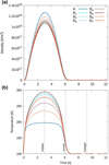 |
Fig. 1 Inlet conditions in the case of a spherical nucleus. Diurnal variation in gas number density (a) and temperature (b) at the nucleus surface in the equatorial plane for the different models considered. |
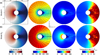 |
Fig. 2 Gas fields in the case of a spherical nucleus. Cross section in the equatorial plane of (from left to right) the gas density, speed (with streamlines), overall temperature, and the ratio of rotational to translational temperature fields (Trot/Ttrans) obtained for Model A (a) and Model B5 (b). The color bars are identical for the two models. |
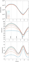 |
Fig. 3 Results for the spherical nucleus. Comparison of the longitudinal variation in the number density (top), the speed (middle), and the overall temperature (bottom) of the gas at a distance of 9 km from the center of the nucleus in the equatorial plane for the different models. |
Mesh properties.
Model properties.
3 Results and discussion
Results on gas fields and spectral lines are presented for different properties of the porous layer. The corresponding models are listed in Table 3. Model A corresponds to the absence of a dust layer and is equivalent to exposed water ice. For Model B, different grain sizes (d), porosities (ϕ), and thicknesses (L) of the dust layer are considered. We first look at the case of a spherical shape, which, because of its symmetries, facilitates the comparisons. We then look at the case of a complex shape for which a direct comparison with MIRO observations is provided.
3.1 Spherical nucleus
Figure 1 shows the inlet conditions for the spherical nucleus. Gas density (top panel) and temperature (low panel) are presented as a function of local time for the equatorial plane. As the production rate is normalized to give an overall mass production of 200 kg/s, the difference in density between the different models is solely related to the difference in surface temperature (Eq. (4)) and we can see that the density changes within about 20 percent only (Fig. 1a). The highest density is expectedly obtained for Model A. The temperature distribution in the layer depends on the (dimensional) thickness of the layer and not on its relative thickness L/d (in monomer diameters; Skorov et al. 2024b).
Therefore, its variations are significant (Fig. 1b). Even if we exclude the lowest temperature obtained in Model A, the average temperature of the emitted molecules changes from about 220 K to 290 K. In this case, not only the layer thickness matters, but also its porosity. Skorov et al. (2024b) studied in detail the dependence of the distribution of the depth of the last collision of molecules with the dust skeleton on the structural parameters of the layer.
Cross sections in the equatorial plane of a inner gas coma are shown in Fig. 2. We present results obtained for Model A (Fig. 2a) and Model B5 (Fig. 2b). The fields of the gas number density, speed (with streamlines), overall temperature and the ratio of the rotational temperature Trot to the translational temperature Ttrans are shown from left to right. For a better comparison, the color bars are identical for the two models. Looking at the density fields we can conclude that their structure is very similar. For Model A, a higher density is observed in the illuminated hemisphere, which is the natural consequence of the higher density at the nucleus surface discussed above. All the main features remain in place, including the “whiskers” in the vicinity of the terminator and the low-density region in the shadow of the nucleus. Comparison of the speed fields does not bring any surprises. In Model B5 the speed at the surface is higher than in Model A, which is a result of the higher gas temperature. This excess of speed only increases in the whole of the illuminated hemisphere. Above the nightside hemisphere of the nucleus in both cases there is a pronounced region of slow flow corresponding to the low-density region. Remembering that in our models the gas production on the unlit side is zero (there is no thermal memory in the models), this region, especially in the vicinity of the nucleus, is filled with molecules that have migrated here from the denser regions of the coma. This is confirmed by the streamlines plotted above the speed fields. At the same time, the efficiency of such a migration is significantly suppressed by the high macro-velocity of the expanding gas flow. Looking at the overall temperature fields, it can be seen that the gas temperature in Model B5 remains higher in almost the entire sun-facing hemisphere up to the outer boundary of the computational domain. From the present illustration it can be expected that the described differences will appear in the analysis of the observations. Finally, the ratio of the rotational temperature (Trot) to the translational temperature (Ttrans) indicates a region of equilibrium (Trot/Ttrans ≃ 1) on the dayside, reflecting better conversion of energy. On the nightside, where collisions are less frequent, a nonequilibrium region appears, dominated by rotational energy.
For a more detailed quantitative comparison of the model results, Fig. 3 shows the longitudinal variation of the properties of the gas, in the equatorial plane, at a constant distance of 9 km from the center of the nucleus. At such a distance, we can see that the density profiles for the various models of type B are very similar and lower than the density profile for Model A. The initial difference at the nucleus surface has increased and is now on the order of 50%, which can be explained by a higher expansion speed. As far as the speed is concerned, we see a much flatter profile in the case of Model A, with relatively little variation apart from in the region behind the nucleus, where the speed is lower. We also find that the models for which the velocity is highest are those for which the nucleus temperature was higher, which is consistent with a better conversion from internal energy of water molecules to kinetic energy. Regarding overall temperature, we observe a smaller difference between the profiles than that observed at the inlet. We also note the presence of two peaks of roughly equal intensity but of different origins. The first, at subsolar longitude, is a remnant of the surface peak, while the second, at the rear of the comet, is due to the convergence of flows from opposite sides of the nucleus.
Before looking at the spectral lines, Fig. 4 compares the radial evolution of the gas fields along two LOSs corresponding to two different phase angles. Figure 4a first shows the vertical profiles at a phase angle of 0°, along the subsolar direction. There is a narrowing of the gap between the density profiles with altitude, linked to a greater acceleration of the least dense gases at the surface, which are also the warmest. Similarly, the temperature profiles become closer with altitude. For a phase angle of 90° (Fig. 4b) there is a density peak at a distance of around 1 km from the nucleus, slightly more intense in the case of Model A. This comes from the flow from the dayside to the nightside. Apart from this, there is no clear trend between the different profiles, apart from a slightly different temperature in the case of Model A, associated with a lower relative velocity.
Finally, Fig. 5 shows the spectral lines for the 110−101 fundamental ortho-rotational line transition and obtained for the isotopologue H216O at 556.937 GHz (left) and H218O at 547.676 GHz (right). An ortho-to-para water of 3:1 (Lee et al. 2015) and an H216O/H218O abundance ratio of 445 (Schroeder et al. 2019) are used in the radiative transfer calculation. As we will see later in the comparison with MIRO observations, observing nearby spectral lines generally helps reduce optical depth effects such as saturation (Thomas 2020). We first considered the case of a phase angle of 0° (Fig. 5a). For comparison, a background temperature Tback = 200 K, representing the continuum brightness temperature from the nucleus, was imposed on all models. This value corresponds to the subsolar surface temperature in Model A. In the presence of a dust layer, the depth of the absorption band decreases and there is a shift toward higher relative velocities, together with a decrease in the depth of the absorption band due to the decrease in gas concentration. In the case of H216O, a red emission wing appears at about +0.5 km/s. Such a feature has been observed at the spring equinox (Marschall et al. 2019) and is explained here by a higher gas temperature than that of the background. The same is true for a phase angle of 90° (Fig. 5b), with a smaller difference between the different models of type B. The background temperature was set here to Tback = 120 K, corresponding to the surface temperature of Model A at the terminator. In this case, the LTE conditions do not necessarily hold (see Fig. 7) and using the total temperature in the radiative transfer calculation may lead to an overestimation of the Doppler broadening and an underestimation of the absorption depth. An emission wing is still observed, but its intensity is lower than in the case of a phase angle of 0°. This emission is also observed for Model A, suggesting that this is due to the contribution of more strongly illuminated zones (Marschall et al. 2019).
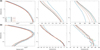 |
Fig. 4 Vertical profiles for the spherical nucleus. Comparison of gas density (left), Doppler velocity (middle), and overall temperature profiles (right) as a function of altitude in the case for a 0° phase angle (a) and a 90° phase angle (b; terminator) for the different models. |
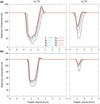 |
Fig. 5 Spectral lines for a spherical nucleus. Comparison of the spectral lines for the 110–101 fundamental line transition for H216O at 556.937 GHz (left) and H218O at 547.676 GHz (right) at a 0° phase angle (a) and a 90° phase angle (b; terminator) for the different models. |
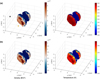 |
Fig. 6 Boundary conditions for the complex shape. Fields of gas density (left) and temperature (right) at the surface of the nucleus in the case of Model A (a) and Model B5 (b) corresponding to the MIRO observation on 2015-07-10T01:32. The direction of the Sun and of the spacecraft are indicated in the top-left panel with an orange star and a black diamond, respectively. |
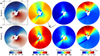 |
Fig. 7 Gas fields obtained for the complex shape. Cross sections of (from left to right) gas density, speed, Knudsen number, overall temperature, and the ratio of rotational to translational temperature fields (Trot/Ttrans) for Model A (a) and Model B5 (b) in the plane containing the nucleus center, Sun, and spacecraft. The color bars are identical for the two models. |
3.2 Complex shape
We next looked at the case of a complex shape. The main objective is to study the effect of the dust layer on the gas fields and to see to what extent this affects the spectral lines in comparison with the one observed by MIRO. For this, we considered the configuration given by the MIRO observations on 2015-07-10T01:32:39, when the phase angle was 89.6°, the subsolar point was located in the Imhotep region, and the MIRO beam was pointing at the Aten/Khepry region of 67P (Table 1). This (near-perihelion) case with cometary activity and a potentially relatively large effect of the dust layer on it has already been considered in Pinzón-Rodríguez (2021), where an arbitrary increase in the gas surface temperature improves the agreement with the spectral lines observed by MIRO. The idea here is to confirm these results by considering a more physically based model.
Figures 6a and b show the input conditions corresponding to Model A and Model B5, respectively (i.e., the gas density at the nucleus surface and its temperature). As in the previous case, the density is slightly lower in the presence of the porous layer, while the temperature is much higher, with a maximum temperature difference of more than 100 K.
We first present the results obtained with the DSMC simulations. Figure 7 compares a cross section (in the plane containing the comet center, the Sun and the spacecraft) of the density, speed, overall temperature, and temperature ratio fields (Trot/Ttrans) obtained for Model A and Model B5. As in the case of the spherical shape, the density fields are quite similar. The speed, which is of the same order of magnitude near the nucleus, increases more rapidly in the presence of the dust layer, indicating a greater conversion of thermal energy into kinetic energy. At the same time, the temperature difference between the models decreases with distance from the comet. Thermal equilibrium (Trot/Ttrans ≃ 1) is observed on the active side of the comet.
To study this more quantitatively, Fig. 8 shows the longitudinal evolution of the gas properties, always in the same plane, at a fixed distance of 9 km from the nucleus. It can be seen that the density remains slightly higher in the case of Model A than in Model B, and the two models have very similar profiles. In terms of speed, there is a greater difference between the models in high-speed areas compared with low-speed areas. As in the case of a spherical nucleus, the speed profile is flatter for Model A. As for temperature, the profiles appear to be fairly similar, with a vertical shift of +5 to +10 K compared with Model A, depending on Model B. Temperature peaks coincide with lower speed zones.
Figure 9 shows the gas, speed and temperature profiles along MIRO’s LOS. Here again, there is very little difference between density profiles. Velocity profiles are close at low altitudes, but greater acceleration is observed in the presence of dust due to warmer gas and conversion of thermal to kinetic energy. This is corroborated by the temperature profiles, where the difference between the models diminishes as the distance from the nucleus increases. A quasi-asymptotic regime, characterized by a weak variation in velocity and temperature with altitude, is thus obtained; the highest relative velocities are obtained for the warmest surface temperatures.
Finally, in Fig. 10 we consider the spectral lines for the 110−101 fundamental ortho-rotational line transition for the isotopologue H216O at 556.937 GHz (left) and H218O at 547.676 GHz (right) obtained for the different models and compare them with the MIRO observations. For the comparison, we consider the background temperature Tback = 185.5 K obtained by MIRO continuum channel. It can be seen that the MIRO spectral line core for the H216O isotopologue is saturated, which is due to optically thick conditions, while the less abundant H218O isotopologue line shape has a well-defined (Doppler) absorption peak. In the following discussion we focus mainly on the Doppler shift velocities of the line core(s) that should signify the terminal expansion velocities (TEVs) of the gas.
We first considered the spectral line of H216O. As shown in Pinzón-Rodríguez (2021), a purely insolation-driven case (Model A) does not fit the MIRO spectra well, with an underestimation of the Doppler velocity for the left (blue shift) wing and an overestimation for the right (red shift) wing. In the presence of a dust layer, a decreasing absorption depth is observed, which is essentially due to the increase in gas temperature. In addition, the higher temperature cases also provide higher gas velocities, and the combination of these two effect provide a better overall agreement with the MIRO spectra (Doppler shift). At this level of analysis the best looking spectrum in terms of Doppler shift and the overall line shape is obtained with Model B6, with very good agreement with the measured TEV (see Table 4).
In the case of the H218O isotopologue, the line core is no longer saturated signifying a smaller optical depth. Similarly to the previous case, the depth of the absorption feature as well as its width decreases in the presence of a dust layer with a proper shifts to the left (higher velocities). In this case, the line depth is in poor agreement with measurements in part due to the simplified assumption of LTE and the actual altitude profile of temperature, which provide the needed contrast in nadir geometry. This can be addressed in the future with updated radiative transfer accounting for non-LTE combined with iterative update of the DSMC. Nevertheless, the TEV estimates in these simulated lines are still valid at this level of analysis. Notably, we observe that the Model B6 Doppler shift is no longer the best estimate, rather the simulations with Model B2 or Model B7 seem to agree better with the MIRO measurement. The numerical values are summarized in Table 4 for all models.
The discrepancy between TEVs estimated from the H216O versus H218O has been already systematically described in Rezac et al. (2021), although no conclusive explanation has been found so far. We can only confirm it here but ultimately our DSMC simulation setup developed in this work cannot address them.
Nevertheless, our modeling did provide a step forward for self-consistent exploitation of information contained in the line shape and Doppler shifts of the MIRO water spectra. First, the near surface coma temperature variance due to the dust layer presence is strongly influencing the formation of red-wing of the H216O, even providing conditions for the often observed emission feature (Marschall et al. 2019). Second, we also demonstrate that using spherical and detailed 67P nucleus models in the DSMC leads to significant differences in the simulated MIRO radiance space. These lessons should be taken into account in future works in order to find self-consistent physical model of cometary coma for 67P.
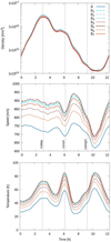 |
Fig. 8 Results for the complex shape. Comparison of the longitudinal variation of the gas number density (top), speed (middle), and overall temperature (bottom) at a distance of 9 km from the nucleus center in the plane containing the nucleus center, Sun, and spacecraft for the different models. |
Terminal expansion velocities.
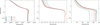 |
Fig. 9 Vertical profiles for the complex shape. Comparison of the gas number density (left), Doppler velocity (middle), and overall temperature (right) along MIRO’s LOS, corresponding to the observation on 2015-07-10T01:32 for the different models. |
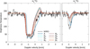 |
Fig. 10 Comparison of simulated (LTE) spectra for the different DSMC variants with MIRO of the spectral lines for the 110-101 fundamental line transition of H216O at 556.937 GHz (left) and H218O at 547.676 GHz (right) corresponding to the observation on 2015-07-10T01:32. |
4 Conclusions
With this study we show how, at a fixed total mass production rate, the presence of a physically justifiable porous layer affects the gas properties in a coma. According to the thermal model considered, the main effect of the porous layer is to increase the temperature of the gas at the surface of the nucleus and decrease its density. We have shown how these initial differences evolve with distance from the surface.
Surface gas temperature differences have a large effect on the magnitude of the temperature and gas velocity in the coma. The main effect is that the gas heated by the porous layer has a greater acceleration due to the conversion of thermal energy into kinetic energy. The result is a reduction in the density differences between the different models, with the densest gases being the least hot, and a higher terminal expansion velocity for the hotter gases. This, although resulting in small differences in gas density over large distances between models, has a major effect on the water absorption lines observed with MIRO. The main result is that the effect of the porous layer on gas properties can be distinguished by comparing spectral lines.
In this work we considered only a few sample MIRO observations that coincide well with our model production rates. For the MIRO observations considered here, the best fit of the spectral line of H216O appears to be Model B6: a dust layer with a grain size of 1 mm, a porosity of 0.75, and a thickness of 10 mm. The H218O line requires a higher terminal expansion velocity, best captured by Model B2 or Model B7. This difference cannot be simply explained by the dust-layer presence, and additional physics should be considered in future works. We hope that this work will lead to a more extensive and systematic exploitation of MIRO data using self-consistent DSMC models.
More generally, the question is to what extent comparison with MIRO spectral lines can be used to infer physical constraints on porous layer properties. This study is only a first step in this direction, since many effects, such as thermal conductivity (Pinzón-Rodríguez et al. 2021), source distribution (Marschall et al. 2020a; Mokhtari & Thomas 2024), and heterogenous activity (Combi et al. 2020), need to be taken into account.
The next step is to consider a larger set of MIRO data to see how our conclusions (in terms of which porous layer provides the best fit) vary with the observational geometry. Mass loss distribution models should be considered to see to what extent heterogeneous activity affects the spectral lines and how precisely it can be constrained via comparisons with MIRO data.
Acknowledgements
This work has been carried out within the framework of the NCCR PlanetS supported by the Swiss National Science Foundation under grants 51NF40_182901 and 5INF40_205606. Yu.S. acknowledges support from ESA through contract 4000141229/23/ES/CM and the Deutsche Forschungsgemein-schaft (DFG) for support under grant BL 298/32-1. Yu.S. and O.M. thank the International Space Science Institute (ISSI) of Bern for the support of this work.
References
- Acton, J., & Charles, H. 1996, Planet. Space Sci., 44, 65 [CrossRef] [Google Scholar]
- Alexander, F. J., & Garcia, A. L. 1997, Comput. Phys., 11, 588 [NASA ADS] [CrossRef] [Google Scholar]
- Bentley, M. S., Schmied, R., Mannel, T., et al. 2016, Nature, 537, 73 [Google Scholar]
- Bird, G. A. 1981, Progr. Astronaut. Aeronaut., 74, 239 [Google Scholar]
- Bird, G. A. 1994, Molecular Gas Dynamics and the Direct Simulation of Gas Flows (Oxford University Press) [Google Scholar]
- Biver, N., Hofstadter, M., Gulkis, S., et al. 2015, A&A, 583, A3 [NASA ADS] [CrossRef] [EDP Sciences] [Google Scholar]
- Borgnakke, C., & Larsen, P. S. 1975, J. Computat. Phys., 18, 405 [NASA ADS] [CrossRef] [Google Scholar]
- Combi, M. R. 1996, Icarus, 123, 207 [NASA ADS] [CrossRef] [Google Scholar]
- Combi, M., Shou, Y., Fougere, N., et al. 2020, Icarus, 335, 113421 [NASA ADS] [CrossRef] [Google Scholar]
- Crifo, J., & Rodionov, A. 1997, Icarus, 129, 72 [NASA ADS] [CrossRef] [Google Scholar]
- Crifo, J., Lukianov, G., Rodionov, A., Khanlarov, G., & Zakharov, V. 2002, Icarus, 156, 249 [NASA ADS] [CrossRef] [Google Scholar]
- El-Maarry, M. R., Groussin, O., Keller, H., et al. 2019, Space Sci. Rev., 215, 1 [CrossRef] [Google Scholar]
- Gerig, S.-B. 2021, PhD thesis, Universität Bern, Switzerland [Google Scholar]
- Gerig, S.-B., Marschall, R., Thomas, N., et al. 2018, Icarus, 311, 1 [NASA ADS] [CrossRef] [Google Scholar]
- Groussin, O., Attree, N., Brouet, Y., et al. 2019, Space Sci. Rev., 215, 1 [CrossRef] [Google Scholar]
- Gulkis, S., Allen, M., Von Allmen, P., et al. 2015, Science, 347, aaa0709 [NASA ADS] [CrossRef] [Google Scholar]
- Gundlach, B., & Blum, J. 2012, Icarus, 219, 618 [CrossRef] [Google Scholar]
- Hansen, K. C., Altwegg, K., Berthelier, J.-J., et al. 2016, MNRAS, 462, S491 [Google Scholar]
- Hässig, M., Altwegg, K., Balsiger, H., et al. 2015, Science, 347, aaa0276 [Google Scholar]
- Kananenka, A. A., & Skinner, J. 2018, J. Chem. Phys., 148 [Google Scholar]
- Keller, H. U., Mottola, S., Davidsson, B., et al. 2015a, A&A, 583, A34 [NASA ADS] [CrossRef] [EDP Sciences] [Google Scholar]
- Keller, H. U., Mottola, S., Skorov, Y., & Jorda, L. 2015b, A&A, 579, L5 [NASA ADS] [CrossRef] [EDP Sciences] [Google Scholar]
- Koura, K., & Matsumoto, H. 1991, Phys. Fluids A: Fluid Dyn., 3, 2459 [NASA ADS] [CrossRef] [Google Scholar]
- Lee, S., Von Allmen, P., Allen, M., et al. 2015, A&A, 583, A5 [NASA ADS] [CrossRef] [EDP Sciences] [Google Scholar]
- Macher, W., Skorov, Y., Kargl, G., Laddha, S., & Zivithal, S. 2024, J. Eng. Math., 144, 2 [NASA ADS] [CrossRef] [Google Scholar]
- Mannel, T., Bentley, M. S., Boakes, P. D., et al. 2019, A&A, 630, A26 [NASA ADS] [CrossRef] [EDP Sciences] [Google Scholar]
- Marboeuf, U., Schmitt, B., Petit, J.-M., Mousis, O., & Fray, N. 2012, A&A, 542, A82 [NASA ADS] [CrossRef] [EDP Sciences] [Google Scholar]
- Marschall, R., Su, C., Liao, Y., et al. 2016, A&A, 589, A90 [NASA ADS] [CrossRef] [EDP Sciences] [Google Scholar]
- Marschall, R., Mottola, S., Su, C., et al. 2017, A&A, 605, A112 [NASA ADS] [CrossRef] [EDP Sciences] [Google Scholar]
- Marschall, R., Rezac, L., Kappel, D., et al. 2019, Icarus, 328, 104 [Google Scholar]
- Marschall, R., Liao, Y., Thomas, N., & Wu, J.-S. 2020a, Icarus, 346, 113742 [CrossRef] [Google Scholar]
- Marschall, R., Skorov, Y., Zakharov, V., et al. 2020b, Space Sci. Rev., 216, 1 [CrossRef] [Google Scholar]
- Mokhtari, O., & Thomas, N. 2024, Icarus, 415, 116072 [NASA ADS] [CrossRef] [Google Scholar]
- Pinzón-Rodríguez, O. 2021, PhD thesis, Universität Bern, Switzerland [Google Scholar]
- Pinzón-Rodríguez, O., Marschall, R., Gerig, S.-B., et al. 2021, A&A, 655, A20 [NASA ADS] [CrossRef] [EDP Sciences] [Google Scholar]
- Pommerol, A., Thomas, N., El-Maarry, M. R., et al. 2015, A&A, 583, A25 [NASA ADS] [CrossRef] [EDP Sciences] [Google Scholar]
- Preusker, F., Scholten, F., Matz, K.-D., et al. 2017, A&A, 607, L1 [NASA ADS] [CrossRef] [EDP Sciences] [Google Scholar]
- Rezac, L., Zorzi, A., Hartogh, P., et al. 2021, A&A, 648, A21 [Google Scholar]
- Rubin, M., Fougere, N., Altwegg, K., et al. 2014, ApJ, 788, 168 [NASA ADS] [CrossRef] [Google Scholar]
- Russell, H. 1935, J. Am. Ceram. Soc., 18, 1 [CrossRef] [Google Scholar]
- Schroeder, I. R., Altwegg, K., Balsiger, H., et al. 2019, A&A, 630, A29 [NASA ADS] [CrossRef] [EDP Sciences] [Google Scholar]
- Skorov, Y., Rezac, L., Hartogh, P., & Keller, H. U. 2017, A&A, 600, A142 [NASA ADS] [CrossRef] [EDP Sciences] [Google Scholar]
- Skorov, Y., Markkanen, J., Reshetnyk, V., et al. 2023, MNRAS, 522, 4781 [NASA ADS] [CrossRef] [Google Scholar]
- Skorov, Y. V., Mokhtari, O., Macher, W., et al. 2024a, A&A, 689, A131 [NASA ADS] [CrossRef] [EDP Sciences] [Google Scholar]
- Skorov, Y., Reshetnyk, V., Markkanen, J., et al. 2024b, MNRAS, 527, 12268 [Google Scholar]
- Su, C.-C. 2013, PhD thesis, National Chiao Tung University, Taiwan [Google Scholar]
- Sunshine, J., A’hearn, M., Groussin, O., et al. 2006, Science, 311, 1453 [NASA ADS] [CrossRef] [Google Scholar]
- Tenishev, V., Combi, M. R., & Rubin, M. 2011, ApJ, 732, 104 [Google Scholar]
- Thomas, N. 2020, An Introduction to Comets: Post-Rosetta Perspectives (Springer Nature) [CrossRef] [Google Scholar]
- Thomas, N., Davidsson, B., El-Maarry, M. R., et al. 2015, A&A, 583, A17 [NASA ADS] [CrossRef] [EDP Sciences] [Google Scholar]
- Wu, J.-S., & Lian, Y.-Y. 2003, Comput. Fluids, 32, 1133 [Google Scholar]
- Wu, J.-S., & Tseng, K.-C. 2005, Int. J. Numer. Methods Eng., 63, 37 [NASA ADS] [CrossRef] [Google Scholar]
- Wu, J.-S., Tseng, K.-C., & Wu, F.-Y. 2004, Comput. Phys. Commun., 162, 166 [NASA ADS] [CrossRef] [Google Scholar]
- Zakharov, V., Rodionov, A., Fulle, M., et al. 2021, Icarus, 354, 114091 [NASA ADS] [CrossRef] [Google Scholar]
Like the vast majority of thermophysical models of the cometary nucleus, we assumed that the albedo is independent of the angle of incidence of the radiation. This assumption is a strong idealization and needs to be revised in the case of a body of complex shape such as 67P (Thomas 2020) especially in the case of heterogeneous surfaces (with ice outcrops). In our next work this effect will be studied quantitatively.
By Plasma T.I, http://plasmati.com.tw
All Tables
All Figures
|
Fig. 1 Inlet conditions in the case of a spherical nucleus. Diurnal variation in gas number density (a) and temperature (b) at the nucleus surface in the equatorial plane for the different models considered. |
| In the text | |
|
Fig. 2 Gas fields in the case of a spherical nucleus. Cross section in the equatorial plane of (from left to right) the gas density, speed (with streamlines), overall temperature, and the ratio of rotational to translational temperature fields (Trot/Ttrans) obtained for Model A (a) and Model B5 (b). The color bars are identical for the two models. |
| In the text | |
|
Fig. 3 Results for the spherical nucleus. Comparison of the longitudinal variation in the number density (top), the speed (middle), and the overall temperature (bottom) of the gas at a distance of 9 km from the center of the nucleus in the equatorial plane for the different models. |
| In the text | |
|
Fig. 4 Vertical profiles for the spherical nucleus. Comparison of gas density (left), Doppler velocity (middle), and overall temperature profiles (right) as a function of altitude in the case for a 0° phase angle (a) and a 90° phase angle (b; terminator) for the different models. |
| In the text | |
|
Fig. 5 Spectral lines for a spherical nucleus. Comparison of the spectral lines for the 110–101 fundamental line transition for H216O at 556.937 GHz (left) and H218O at 547.676 GHz (right) at a 0° phase angle (a) and a 90° phase angle (b; terminator) for the different models. |
| In the text | |
|
Fig. 6 Boundary conditions for the complex shape. Fields of gas density (left) and temperature (right) at the surface of the nucleus in the case of Model A (a) and Model B5 (b) corresponding to the MIRO observation on 2015-07-10T01:32. The direction of the Sun and of the spacecraft are indicated in the top-left panel with an orange star and a black diamond, respectively. |
| In the text | |
|
Fig. 7 Gas fields obtained for the complex shape. Cross sections of (from left to right) gas density, speed, Knudsen number, overall temperature, and the ratio of rotational to translational temperature fields (Trot/Ttrans) for Model A (a) and Model B5 (b) in the plane containing the nucleus center, Sun, and spacecraft. The color bars are identical for the two models. |
| In the text | |
|
Fig. 8 Results for the complex shape. Comparison of the longitudinal variation of the gas number density (top), speed (middle), and overall temperature (bottom) at a distance of 9 km from the nucleus center in the plane containing the nucleus center, Sun, and spacecraft for the different models. |
| In the text | |
|
Fig. 9 Vertical profiles for the complex shape. Comparison of the gas number density (left), Doppler velocity (middle), and overall temperature (right) along MIRO’s LOS, corresponding to the observation on 2015-07-10T01:32 for the different models. |
| In the text | |
|
Fig. 10 Comparison of simulated (LTE) spectra for the different DSMC variants with MIRO of the spectral lines for the 110-101 fundamental line transition of H216O at 556.937 GHz (left) and H218O at 547.676 GHz (right) corresponding to the observation on 2015-07-10T01:32. |
| In the text | |
Current usage metrics show cumulative count of Article Views (full-text article views including HTML views, PDF and ePub downloads, according to the available data) and Abstracts Views on Vision4Press platform.
Data correspond to usage on the plateform after 2015. The current usage metrics is available 48-96 hours after online publication and is updated daily on week days.
Initial download of the metrics may take a while.