| Issue |
A&A
Volume 630, October 2019
Rosetta mission full comet phase results
|
|
|---|---|---|
| Article Number | A34 | |
| Number of page(s) | 8 | |
| Section | Planets and planetary systems | |
| DOI | https://doi.org/10.1051/0004-6361/201935389 | |
| Published online | 20 September 2019 | |
Three-dimensional analysis of spatial resolution of MIRO/Rosetta measurements at 67P/Churyumov-Gersimenko
1
Max-Planck-Institut für Sonnensystemforschung,
Justus-von-Liebig-Weg 3,
37077 Göttingen,
Germany
e-mail: rezac@mps.mpg.de
2
Key Laboratory of Planetary Sciences, Purple Mountain Observatory, Chinese Academy of Sciences,
Nanjing 210008, PR China
3
CAS Center for Excellence in Comparative Planetology, Chinese Academy of Sciences,
PR China
Received:
4
March
2019
Accepted:
2
May
2019
Context. The MIRO instrument’s remote sensing capability is integral to constraining water density, temperature, and velocity fields in the coma of 67P/Churyumov-Gersimenko.
Aims. Our aim is to quantify how much water density originates from the facets of the shape model within the field of view of MIRO versus the water contribution from all the other facets. This information is crucial to understanding the MIRO derived coma production rates and their relation to the nucleus characteristics, and to understanding the spatial resolution of the measurements.
Methods. This study relies on a detailed 3D nucleus shape model, illumination conditions, and the pointing information of the viewing geometry. With these parameters we can evaluate the relative contribution of water density originating from facets directly inside the MIRO beam and outside the beam as a function of distance along the MIRO line of sight. We also calculate the ratio of in-beam versus out-of-beam water gas number density.
Results. We demonstrate that despite the rather small MIRO field of view there is only a small fraction of molecules that originate from facets within the MIRO beam. This is true for the nadir, but a similar conclusion can also be applied to the limb observing geometry.
Conclusions. The MIRO instrument cannot discriminate active from inactive regions directly from observations. This study also suggests that the beam averaged solar incidence angle, local time, and mean normal vectors are not necessarily related to molecules within the MIRO beam. These results also illustrate why the 1D spherical Haser model can be applied with relative success to analyzing the MIRO data (and generally any Rosetta measurements). The future possibilities of constraining gas activity distribution on the surface should use 3D codes extracting information from the MIRO spectral line shapes which contain additional information. The results presented here are applicable to remote sensing instruments on board Rosetta.
Key words: comets: general / comets: individual: 67P/CG
© L. Rezac et al. 2019
 Open Access article, published by EDP Sciences, under the terms of the Creative Commons Attribution License (http://creativecommons.org/licenses/by/4.0), which permits unrestricted use, distribution, and reproduction in any medium, provided the original work is properly cited.
Open Access funding provided by Max Planck Society.
1 Introduction
The Microwave Instrument for the Rosetta Orbiter (MIRO) consisted of a 30 cm primary dish followed by two heterodyne receivers operating at center frequencies of 190 and 562 GHz (Gulkis et al. 2007). It was one of the four remote sensing instruments (the others being OSIRIS, VIRTIS, and ALICE)1 on board Rosetta that shared the science goal of monitoring the onset of cometary activity and its evolution through the perihelion passage (August 13, 2015). The 562 GHz MIRO receiver was designed to be sensitive to radiation at submillimeter wavelengths that are characteristic of molecular emissions due to transitions between rotational states of molecules. This MIRO receiver was also connected to a high-resolution Chirp Transform Spectrometer (CTS; Hartogh & Hartmann 1990), tuned to record eight spectral lines of six important species present in the coma (H O, H
O, H O, H
O, H O, CO, NH3, and three lines of CH3OH). The CTS provided a high-frequency resolution (R ~ 1 × 10⁷), such that individual spectral line shapes could be accurately determined. These line profiles carry information about the variation in expansion velocity, temperature structure (especially for optically thick transition), and density profile along the line of sight (LOS). In general, the MIRO geometry provides two modes of observations, boresight on the nucleus surface (nadir) where the spectra are seen in absorption against the warmer nucleus (compared to the coma), and “limb” where the lines are seen in emission against the background of cold space (cosmic background radiation), see Fig. 1. However, because of the finite extent of the MIRO beam (half power beam width, HPBW ~ 420”), there are cases where one portion of the beam sees the cold space and the other sees the warm nucleus, resulting in mixed spectra features. As we discuss and quantify in this paper, there are fundamental problems when interpreting the MIRO data in terms of resolving possible activity spots on the nucleus, and when relating beam averaged information on incidence and emission angles to the derived gas column densities.
So far, all MIRO data analysis have relied on the simplified framework of 1D Haser model in spherical symmetry (Haser 1957). The 1D idealization has been a practical way to obtain the first results, especially in constraining the total water production rates which are derived from the line area of the spectra (Gulkis et al. 2015). Additional complexity favoring the 1D approach for MIRO spectra interpretation is needed to account for non-local thermodynamic equilibrium (non-LTE) effects in rotational level populations. Calculations of rotational population in 3D geometry is a nontrivial and very time consuming task.
The very first results of MIRO regarding production rates are discussed in Gulkis et al. (2015) and Biver et al. (2015), noting that the “neck” (Hapi) region El-Maarry et al. (2015) always yields the largest observed production rates. In the work of Lee et al. (2015) MIRO nadir observations from August 7 to 19, 2014 were studied, along with a correlation of production rates with local time and illumination condition. Within the assumptions of their retrieval approach, they found a strong spatial variation in outgassing (from (0.1 to 3) × 1025 mol s−1), but no direct correlation with illumination conditions at the surface of the nucleus within MIRO’s field of view (FOV). Marshall et al. (2017) analyzed the spatial pattern of variation as a function of heliocentric distance taking into account nearly the entire MIRO database of nadir geometries. That study also provided an estimate of the total production rate and its peak offset (22–46 days) with respect to perihelion.
In this work we investigate the relationship between water density at a given grid point (or sampling point) along the MIRO LOS (withinits FOV) and the pattern of illumination-driven surface outgassing. This has a very important implication for several still open questions: (1) whether MIRO can accurately discriminate active from inactive regions on the nucleus (and their spatial scales), (2) how well local illumination conditions (e.g., local time) evaluated from facets within the beam reflect the most likely sourceof detected gas molecules in the MIRO beam, and (3) how well the 1D spherical model can represent the 3D nature of the water source distribution on the surface. We consider both the nadir and limb geometry observations.
The paper is structured as follows. In Sect. 2 we gives a description of our model and explanation of geometry. In Sect. 3 we present the main results and discussion for different geometries. In Sect. 4 we provide the summary and recommendation for future MIRO spectra interpretation.
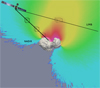 |
Fig. 1 Schematic illustration of the two primary observational geometry of MIRO, (a) nadir and (b) limb, as labeled. The typical spacecraft cometocentric distance is of ~100 km. The cubic volumes placed at a few points along the line of sight symbolize a model grid point inside the MIRO FOV. Despite therather small FOV of MIRO, each grid point can receive molecules from different visible regions of the nucleus. Sizes and distances are not to scale. The color-coding shows modeled water density on one cross section through the coma. |
2 Modeling
2.1 Shape model
The shape of the 67P/Churyumov-Gersimenko (67P) nucleus is approximated with a 3D digital terrain model SHAP7 with 125 000 facets using stereophotogrammetry (SPG; Preusker et al. 2017). In this model each facet has an area of around 235 m2 and the two neighboring vertices are about 12 m apart. At a typical spacecraft distance of 100 km the MIRO footprint has an area of approximately 31 000 m2. Hence, this resolution is sufficient to obtain accurate information on the distribution of all facets contributing to the MIRO beam for a given viewing geometry.
2.2 3D coma model
The surface boundary condition specifying the molecular flux from each facet is determined by a basic energy balance:
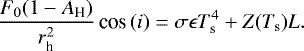 (1)
(1)
This is the same approach as in model A of Keller et al. (2015). The quantities have their usual meaning of solar flux at 1 au distance, F0, scaled by proper heliocentric distance, rh, and the cosine of solar incidence angle, i, for a given facet. Similarly to Marschall et al. (2019), we set the hemispheric albedo to 0.04 and emissivity ϵ to 0.9. Here L is the latent heat of sublimation of water, Z(Ts) is the mass loss flux, Ts is the boundary (surface) temperature, and σ is the Stefan–Boltzmann constant. In this work the absolute water fluxes are of no concern to us; instead, we normalize the surface fluxes emanating from each facet with respect to the maximum value for a given conditions. Realistic water fluxes for each surface element of the nucleus may require a simultaneous 3D inversion of several Rosetta datasets (including MIRO), as was attempted with the ROSINA data (Kramer et al. 2017). Nevertheless, an effort of this kind has not yet been shown to yield a unique solution (Marschall et al. 2017, 2019).
The outflow velocity from each facet is determined by the surface equilibrium temperature (see Eq. (1)). For each facet, molecules escape uniformly into a hemisphere, 2π (srad), but accounting for topographical obstacles in a purely geometrical fashion. Our coma model is collisionless, effectively a Boltzmanntransport equation without force and collision terms. The water density at a given coma grid point (along the MIRO LOS) is obtained as the sum of contributions over all visible facets, as illustrated in Fig. 2.
The simplified assumptions in this coma model do not strongly influence our results, as we discuss below. First, we neglect the conduction term into the surface in our energy balance equation, and ice activity is assumed to originate at the surface. This means that we have instantaneous adjustment of energy at the surface (effectively zero thermal inertia). This provides an upper limit on the water outgassing from illuminated facets. Nevertheless, since we are not interested in absolute values, we normalize the calculated fluxes by the maximum flux from a facet at the given sampling grid point. Second, the coma model is collisionless, which impacts the flow pattern near the nucleus (depending on the production rates), and hence the density distribution. However, differences between a collisionless model and a collisional one (e.g., derived with a DSMC code) in absolute water densities at a certain radial distance are on the order of 20% (Kramer et al. 2017). In reality, a much larger uncertainty in absolute molecular fluxes originates from our complete lack of knowledge regarding which facets are active or inactive at any given illumination and observational geometry.
On the other hand, this model is expected to underestimate the smearing of different surface sources that collisions (effectively a scattering process) inherently introduce. Nevertheless, our goal is to illustrate that even the small FOV of MIRO does not guarantee that molecules at a given height along the LOS originate locally within the beam. This will become clear even when we neglect the effects that smearing and smoothing collisions introduce.
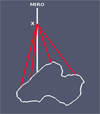 |
Fig. 2 Contribution of different surface elements to a grid point, X, along the LOS of MIRO beam. Despite the small FOV of MIRO, a grid point along the LOS may receive a contribution from nearly the entire surface. The points farther away from the surface have a larger spatial domain from which they may obtain contribution. |
2.3 Sample points selection
Our goal is to get a sense of the spatial (horizontal) extent of contributions of [H2O] along the MIRO LOS (as illustrated in Fig. 2). In this section we show figures for several selected grid points (2.5, 5, and 20 km) along the MIRO LOS. Finally, we also calculate the entire column density of water arising just from facets within the FOV and compare them to the value derived from the contribution from all other facets.
The number density cumulative distribution function obtained from the 1D Haser model of outgassing indicates that about 90% of the molecules are within the first 10 km and 95% within 20 km distance from the nucleus surface. In part, this drives our choice of the 20 km point. In addition, we considered a more detailed argument from the physics of H2O line formation that MIRO measures. Usually, the optically weak H O line, is used to estimate the in-beam column density of water, which is then used for production rate assessment (Gulkis et al. 2015; Biver et al. 2015). In Fig. 3 we plot the nadir contribution functions showing from which heights along the MIRO LOS the measurements are most sensitive to changes in water density; these sensitivity functions are usually called Jacobians (Rodgers 2000). In this example we used a 1D non-LTE transfer code (Marshall et al. 2017; Yamada et al. 2018) applicable to cometary atmosphere with a Haser production rate of 2 × 1026 mol s−1. The line center is Doppler shifted to approximately − 0.79 km s−1 and its corresponding peak sensitivity is at an altitude of approximately 8 km. However, we note that the contribution function is broad and the sensitivity is non-negligible in the altitude range of 1–40 km. Similarly, in the line wing (e.g −0.44 km s−1) the peak sensitivity is closer to the surface, around 2 km altitude, but a non-negligible contribution covers regions roughly from 500–4000 m. The particular vertical structure of these functions reflects the physics of the radiative transfer and LOS profiles of velocity, density, and temperature. In all cases the selected grid points (2.5, 5, and 20 km) are selected on these physical principles to obtain a good understanding of how the MIRO measurement is affected differently along the LOS. The main principle seems obvious, the farther away a grid point from the surface, the larger the number of visible facets that have the potential to contribute molecules (see Fig. 2).
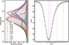 |
Fig. 3 Left: Nadir Jacobians for the H |


3 Results and discussion
For several practical reasons the Rosetta spacecraft was kept approximately on the terminator orbit for extended periods of time. In such an orbit the subspacecraft point follows the morning or evening shadow lines as the nucleus rotates. There are several short periods when the trajectory was selected to cross the subsolar longitude and/or the polar night regions. With these trajectories the spacecraft altitude also changed dramatically (during the near nucleus operations), reaching a cometocentric distance of about 10 km and extending to several hundred kilometers(near perihelion). Therefore, instead of making an artificial choice for illumination, spacecraft position, and attitude, we show a few randomly selected examples from the MIRO observational database. The nucleus illumination and MIRO geometry in all the presented cases are calculated for a given time from the provided SPICE kernels2 using the SPICE library3 (Acton 1996).
The list of examples is shown in Table 1, along with information on the geometry and spacecraft cometocentric distance.
Log of selected cases.
3.1 Nadir study cases
We present three cases for nadir geometry, each with different MIRO pointing and nucleus illumination. In each figure, the camera in panels A–D is located at the spacecraft position with the focus set at the intersection of the MIRO beam center and the nucleus. The camera FOV (panels B–D) is set to about 3° to show the entire nucleus and the surface distribution in better detail. The color bar relevant for panels B–D is shown in the middle of the figurein log color scale from 1 to 0.01. As previously noted the water density is scaled by the maximum water flux to a given grid point for a given geometry.
In each figure, panel A shows the illumination on the shape model with a MIRO beam size as the red circle. In panel B, the shape modeldisplays each facet’s contribution to the grid point 2.5 km from the surface lying on the LOS of MIRO beam. The yellow vector depicts the direction of the sun, while the white circle represent the proper projected size of the MIRO beam. Panel C shows thesame as (B), but for a grid point at 5 km from the surface, and in (D) the point is at 20 km from the surface along the MIRO LOS.
In case 1, the MIRO beam is pointing toward the center of the Imhotep region (Fig. 4). In panel B, the coma grid point is located at 2.5 km from the surface (beam-surface intersection), and we see that already in this consideration that a rather large area around the beam FOV may be contributing. Nevertheless, we consider that the water density at the 2.5 km grid point is still locally determined. However, the water density at sampling grid points at 5 and 20 km (panel C and D, respectively) includes contributions from a very large area. A grid point at 20 km may be considered to receive contributions from almost the entire Imhotep region. It includes even a small fraction from the small lobe visible at the grid point. The ratio of water column density from all facets within the MIRO FOV compared to the rest of the facets outside the FOV is less than 1% starting already at 2.5 km.
In Fig. 5, the viewing geometry puts the MIRO beam on the small lobe nearly at the terminator. As in previous cases, it is clear that different points along the LOS receive a contribution from rather different regions of the nucleus (compare panels B–D). In this particular geometry, the grid point at 2.5 km distance from the surface (panel B) turns out to have a rather small region of contribution. However, at 5 km and finally at 20 km distance the water molecules may come from extended and rather different regions (significant contributions can even come from the other lobe). Also, in this example the ratio of in-beam to out-of-beam water column density is much lower than 1%.
Figure 6 provides another example for a different viewing geometry. The description and conclusions are the same as presented previously. The only small exception to note here is that at a distance of 2.5 km (panel B) the contributing region is visibly offset from the beam with larger area coverage as well, and it is not as small as in the previous example.
These results have a far reaching consequence when considering MIRO gas coma measurements in nadir geometry. First, it is now clear that estimating local time, emission angles, or average normal vector (as it relates to estimates of gas emission direction) by considering only facets within the beam may result in ignoring nucleus regions that in reality may be the strongest sources of water molecules on the MIRO LOS. It is likely that the early MIRO results (Q[H2O] of a few ×1026) (Lee et al. 2015) where a very weak correlation of water column with local time (derived from facets within the MIRO beam) was reported, suffer from the presented effects. Second, when MIRO averaged spectra at intervals of 30–60 min are considered the smearing of different regions contributing to the LOS may be very strong; for the correct interpretation of possible local source regions the presented analysis should be performed. Third, it is now also clear why, despite the small MIRO FOV, we cannot really discriminate active from inactive surface regions, at the scale of MIRO footprint, based on individual measurements. This lack of evidence of inactive regions lead to the general acceptance that the entire surface of 67P is more or less active (e.g., Keller et al. 2017). However, it appears that the Rosetta instruments designed to measure the gas coma may fundamentally not be able to directly confirm this interpretation, namely MIRO nadir geometry observations. Finally, these plots also provide an explanation of why the 1D Haser approximations used in many works do a quite reasonable job of explaining the measurements. At a far enough distance, nearly the entire visible surface could be considered a source of water vapor (accounting for illumination), which by the physics of expansion and smearing of different regions approximates the hemispheric Haser outgassing.
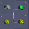 |
Fig. 4 Case 1: illumination conditions for a given time stamp (panel A). Panels B–D: surface distributions of H2O density originating from different facets into the MIRO LOS at selected grid points 2.5, 5, and 20 km from the surface. The red circle in (A) and white dots in (B–D) indicate the footprint of MIRO’s sub-millimeter beam (see text for details). |
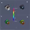 |
Fig. 5 Case 2: illumination conditions for a given time stamp (panel A).Panels B–D: surface distributions of H2O density originating from different facets on the MIRO LOS at selected grid points 2.5, 5, and 20 km from the surface (see text fordetails). |
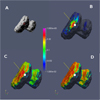 |
Fig. 6 Case 3: illumination conditions for a given time stamp (panel A). Panels B–D: surface distributions of H2O density originating from different facets on the MIRO LOS at selected grid points 2.5, 5, and 20 km from the surface (see text fordetails). |
3.2 Limb study cases
Here we present limb cases that demonstrate the surface contribution to the MIRO LOS when the boresight is pointing off the nucleus. For interpretation we will distinguish anterior and posterior points relative to the tangent point. In the limb geometry the tangent point refers to a point along the LOS lying closest to the surface. Although the bi-lobed shape makes this spherical definition problematic in special cases, we adopt it here as it does not influence our interpretation of results. The ante (before) tangent point refers to grid points lying on the LOS segment from spacecraft to the tangent point, and post (after) refers to the segment from tangent point onward, away from the spacecraft.
Similarly to the nadir cases, the limb cases are presented as four panel plots (Figs. 7 and 8), with panel A showing the nucleus orientation and illumination as viewed from the spacecraft. Panels B–D all have the same camera setting, focus, and FOV (3°), as discussed previously. Panel B shows the relative contribution of facets to the grid point at around 6 km from the tangent point closer to thespacecraft (ante). To better illustrate the results, the nucleus in panels C and D is rotated to show the visible hemisphere containing the MIRO LOS, which is also plotted as a straight line. It should be kept in mind that the images only display a projection of the 3D LOS so it is not so easy to judge distances and orientations, but it gives us reasonable context. The spacecraft icon illustrates the direction of the spacecraft, so that its easy to describe anterior and posterior tangent points for which these distributions are plotted. Hence, panel C shows contributions to the grid point 6 km before the tangent point, while panel D shows the same for grid point 6 km after the tangent point. In the limb geometry, this entire segment (±6 km) provides a large fraction of total molecules within the MIRO beam, but not all. However, we will neglect showing other points along the LOS since the main message is already conveyed in the figures presented below.
Case 4 (Fig. 7) is for off-nucleus pointing with a tangent point at about 2 km above the surface, with the illuminationcoming from the top right corner (see panel A). The illumination is such that extensive regions from both lobes contribute significantly to this point. On the other hand, panel D shows the pattern of contribution to the opposite 6 km grid point (posterior to the tangent point). Here we see that facets on the larger lobe do not contribute that much due to the topography blocking the facet’s view of this grid point. As might be expected, this is one of the geometries where the anterior and posterior points along the LOS receive contributions from rather diverse regions.
In the example of case 5 (Fig. 8), MIRO is viewing above the illuminated southern hemisphere region. Panels C and D provide views of the rotated nucleus to better demonstrate the extensive surface contribution to the anterior and posterior 6 km grid point on the LOS. As in the previous figure, the anterior and posterior points receive the largest water density contribution from very different regions of the nucleus.
The presented results for the selected cases of limb geometry agree with the conclusions derived for the nadir geometry calculations. In the limb geometry there is an additional feature appearing where segments at opposite sides of the tangent point may actually receive a contribution from very different nucleus regions. Although we present cases for a single line of sight, it is clear that for a fixed nucleus orientation and different tangent point altitudes, the qualitative picture remains unchanged. On the other hand, if the pointing changes significantly during a limb scan sequence (such that different nucleus regions become illuminated), then the spatial smearing is expected to become significant. In such cases the interpretation of and correlation to some morphological regions as the source of activity becomes questionable. As it appears that for limb geometry (at least near the nucleus coma), the water density along the LOS is almost always a mixture of nadir and limb. The nadir would refer to the visible side of the nucleus to some grid point on the LOS within the beam. Hence, from the perspective of estimating column density along the LOS (used for later production rates) the 1D Haser model seems to work because the nucleus is much smaller than the typical spacecraft orbital distance. Under such observing conditions of cometary coma we always find that many different regions contribute to the total column density of MIRO. The logic of this conclusion is valid for several other instruments on board Rosetta.
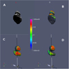 |
Fig. 7 Case 4: illumination conditions for a given time stamp (panel A) along with the projected MIRO beam at the comet distance (red circle). Panel B: contributions to a 6 km grid point before the tangent point keeping the spacecraft view. Panels C and D: grid points 6 km ante and post tangent point respectively, and are oriented to show the relevant part of the nucleus. The LOS has a black segment indicating ±6 km around the tangent point (for details see the description in the text). |
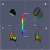 |
Fig. 8 Case 5: illumination conditions for a given time stamp (panel A) along with the projected MIRO beam at the comet distance (as red circle). Panel B: contributions to a 6 km grid point before the tangent point keeping the spacecraft view. Panels C and D: grid points 6 km ante and post tangent point respectively, and are oriented to show clearly the relevant part of the nucleus. The LOS has a black segment indicating the ±6 km distance around the tangent point. For all details see the description in the text. |
4 Summary
In this work we focus on understanding the relationship between the surface activity and water number density along the LOS of the MIRO beam for nadir and limb observational geometry. For this purpose our model accounts for a 3D nucleus shape model, proper illumination conditions, and MIRO viewing geometry for selected cases. The gas flow is treated in the purely noncollisional limit such that water density at a given grid point on the MIRO LOS is determined by the geometry (see Fig. 2). This idealization is not critical for our results. It is not possible to provide absolute numbers since the actual surface water activity is not known on the spatial resolution of individual facets. It is also arguable that any code with proper forces and collisional terms in molecular transfer (such as 3D DSMC) would imply even larger spatial smearing of surface water sources than we report here. This follows considering any two particle collisions to be a scattering event, which results in a multi-scattering problem (like seeing through fog). It is not possible to provide a precise quantitative statement as it depends on the actual outgassing conditions, the collisional rate, and the velocity distribution of the released molecules for each facet.
The main conclusions of this work can be summarized as follows:
-
In general, the contribution of water number density to the MIRO beam is significantly larger from facets outside the FOV than from facets inside the FOV. In our nadir cases the facets inside the FOV contribute less than 1% to the total LOS column density. In Appendix A we present an additional explanation for idealized spherical geometry.
-
In nadirgeometry, different points along the LOS may receive contributions from different regions of the nucleus (grid points below 2 km have the most local contribution relative to the FOV). Grid points at distances of more than about 5 km may receive molecules from virtually the entire visible (and illuminated) surface.
-
In the limb geometry, the larger geometrical path lengths imply even greater smoothing for determining the local regions of activity. The entire visible (and illuminated) fraction of surface contributes (see panels C and D in Figs. 7 and 8). In addition, the anterior and posterior segments relative to the tangent point may receive molecules from vastly different regions (different lobes).
-
In addition, for the nadir geometry, MIRO beam-averaged characteristics of emission angle, solar illumination, local time, or normal vector may not be related to the actual source of water molecules in the MIRO beam. These findings may explain the weak correlation between illumination and water production in Lee et al. (2015).
-
As in the limb geometry, the idea of projecting a tangent point onto the nucleus shape to retrieve illumination conditions at the intersecting point may not necessarily yield the intended information pertaining to the particular observation (see Figs. 7 and 8).
-
This work also sheds more light on why the 1D Haser models applied in MIRO analysis (and other instruments in published works) do a reasonable job of explaining the measurements.
-
It is also clear now that MIRO cannot provide the originally expected information on local activity or inactivity of nucleus regions through direct inversion of individual measurements. This is especially true for periods when the production rate increases and the coma becomes more collisional. However, this does not mean all is lost. With proper 3D modeling, accounting for all the information in the full MIRO line shape, it might be possible to identify in a more local sense the activity of some particular nucleus regions. A multi-instrument study is required to answer this question effectively.
-
Finally, we would recommend caution, based on these results, when attempting correlative studies (models or other Rosetta datasets such as dust jets) with MIRO derived column densities (or production rates), assuming that they originate from the location of the MIRO footprint.
Within the limits of our assumptions of homogeneous solar driven activity and collisionless gas, our results are certainly applicable to MIRO observations. In this work we have not considered the role of individual active spots, for example as identified in Vincent et al. (2016). However, the results presented here provide a clue on how to proceed in the determination of gas activity distributions on the surface. An improvement would be expected from collecting measurements for some identified location from different viewing directions. This inversion would have to be 3D rather than 1D (a spherically symmetric assumption). A numerical study of this 3D method has not yet been performed to demonstrate the feasibility (how small an active area can be uniquely determined) and accuracy of such an approach. In application to the inversion of Rosetta data for surface activity distribution we believe the best physical approach is to account self-consistently for constraints from multiple instruments. For example, the MIRO data provide information on expansion velocity and on temperature profile along each LOS in addition to the water number density profile, and these physical constraints would add another layer of realism to the models.
The results of this work are likely applicable to other Rosetta instruments (remote sensing as well as in situ measurements with wide FOV). As in the case of MIRO, nucleus illumination and characteristics at a subspacecraft point may not be related to the region from which the dominant fraction of detected molecules originate. It follows that directly it is also not possible to make unique identifications of local regions of surface activity.
Acknowledgements
We acknowledge the entire European Space Agency (ESA) Rosetta team, without whom this work could not have been done. Rosetta is an ESA mission with contributions from its member states and NASA. LR received support from the project DFG-392267849 and partly from DFG-HA3261-9/1. Y.Z. was funded by the National Natural Science Foundation of China (Grant No: 11761131008, 11673072, 11633009) and the Foundation of Minor Planets of Purple Mountain Observator. J.J. thanks the National Natural Science Foundation of China (Grant No: 11661161013, 11473073), the Strategic Priority Research Program on Space Science, the Chinese Academy of Sciences (Grant No. XDA15020302), and the CAS interdisciplinary Innovation Team foundation.
Appendix A Solid angle of a spherical sector for a beam and sample points
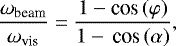
Here we want to outline a simple geometric argument to further support the detailed numerical simulations presented in the main text. To do this we compare solid angles of two spherical sectors. The first spherical sector is formed from projected MIRO FOV (magenta cone in Fig. A.1) onto the nucleus, and the second is due to the entire visible area from a sample point, P, positioned somewhere along the MIRO LOS. In this figure, point O is the comet center, and M is the MIRO (spacecraft) position such that its altitude is D = |MO|− R above the surface. Point P denotes a sample point along the LOS for which we evaluate the visibility limits. The surface distance of P is Z = |PO|− R. The angle φ is  , while cos (α) = R∕(R + Z). The ratio of the solid angle of spherical sector made from the MIRO projected beam to the entire visible sector from point P is
 (A.1)
(A.1)
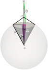 |
Fig. A.1 MIRO instrument positioned at point M with a FOV with half width at half maximum angle, θ. The gray cone is the portion of the spherical nucleus formed from the limits of visibility from point P. The magenta cone is the segment due to the projected MIRO FOV. The distances and angles in this graphic are not to scale. The ratio of solid angles that these cones subtend is given in Eq. (A.2). |
which can be expressed as
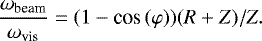 (A.2)
(A.2)
For a comet of radius R = 2 km, the half width at half maximum (HWHM) of MIRO FOV of ~ 1 × 10⁻³ (rad); spacecraft distance, D, of 100 km; and 20 km to the sampling point, Z, the ratio is evaluated at 0.14%. This gives a rough order of magnitude estimate of how much more water we would expect from the area outside the FOV of the MIRO beam. The real ratio might be slightly higher or lower than this geometric ratio of solid angles depending on the detailed shape, morphology of a region, illumination conditions, and actual water activity from each facet. Furthermore, it also would depend on the physics of outgassing (surface sublimation versus subsurface effusion, and the exact velocity distribution).
References
- Acton, C. H. 1996, Planet. Space Sci., 44, 65 [NASA ADS] [CrossRef] [Google Scholar]
- Biver, N., Hofstadter, M., Gulkis, S., et al. 2015, A&A, 583, A3 [NASA ADS] [CrossRef] [EDP Sciences] [Google Scholar]
- El-Maarry, M. R., Thomas, N., Giacomini, L., et al. 2015, A&A, 583, A26 [NASA ADS] [CrossRef] [EDP Sciences] [Google Scholar]
- Gulkis, S., Frerking, M., Crovisier, J., et al. 2007, Space Sci. Rev., 128, 561 [NASA ADS] [CrossRef] [Google Scholar]
- Gulkis, S., Allen, M., von Allmen, P., et al. 2015, Science, 347, aaa0709 [Google Scholar]
- Hartogh, P., & Hartmann, G. K. 1990, Meas. Sci. Technol., 1, 592 [NASA ADS] [CrossRef] [Google Scholar]
- Haser, L. 1957, Bull. Acad. Belg., 43, 740 [Google Scholar]
- Keller, H. U., Mottola, S., Davidsson, B., et al. 2015, A&A, 583, A34 [NASA ADS] [CrossRef] [EDP Sciences] [Google Scholar]
- Keller, H. U., Mottola, S., Hviid, S. F., et al. 2017, MNRAS, 469, S357 [CrossRef] [Google Scholar]
- Kramer, T., Läuter, M., Rubin, M., & Altwegg, K. 2017, MNRAS, 469, S20 [CrossRef] [Google Scholar]
- Lee, S., von Allmen, P., Allen, M., et al. 2015, A&A, 583, A5 [NASA ADS] [CrossRef] [EDP Sciences] [Google Scholar]
- Marschall, R., Mottola, S., Su, C. C., et al. 2017, A&A, 605, A112 [NASA ADS] [CrossRef] [EDP Sciences] [Google Scholar]
- Marschall, R., Rezac, L., Kappel, D., et al. 2019, Icarus, 328, 104 [NASA ADS] [CrossRef] [Google Scholar]
- Marshall, D. W., Hartogh, P., Rezac, L., et al. 2017, A&A, 603, A87 [NASA ADS] [CrossRef] [EDP Sciences] [Google Scholar]
- Preusker, F., Scholten, F., Matz, K.-D., et al. 2017, A&A, 607, L1 [NASA ADS] [CrossRef] [EDP Sciences] [Google Scholar]
- Rodgers, C. D. 2000, Inverse Methods for Atmospheric Sounding: Theory and practice (Singapore: World Scientific) [CrossRef] [Google Scholar]
- Vincent, J.-B., A’Hearn, M. F., Lin, Z.-Y., et al. 2016, MNRAS, 462, S184 [CrossRef] [Google Scholar]
- Yamada, T., Rezac, L., Larsson, R., et al. 2018, A&A, 619, A181 [NASA ADS] [CrossRef] [EDP Sciences] [Google Scholar]
All Tables
All Figures
|
Fig. 1 Schematic illustration of the two primary observational geometry of MIRO, (a) nadir and (b) limb, as labeled. The typical spacecraft cometocentric distance is of ~100 km. The cubic volumes placed at a few points along the line of sight symbolize a model grid point inside the MIRO FOV. Despite therather small FOV of MIRO, each grid point can receive molecules from different visible regions of the nucleus. Sizes and distances are not to scale. The color-coding shows modeled water density on one cross section through the coma. |
| In the text | |
|
Fig. 2 Contribution of different surface elements to a grid point, X, along the LOS of MIRO beam. Despite the small FOV of MIRO, a grid point along the LOS may receive a contribution from nearly the entire surface. The points farther away from the surface have a larger spatial domain from which they may obtain contribution. |
| In the text | |
|
Fig. 3 Left: Nadir Jacobians for the H |
| In the text | |
|
Fig. 4 Case 1: illumination conditions for a given time stamp (panel A). Panels B–D: surface distributions of H2O density originating from different facets into the MIRO LOS at selected grid points 2.5, 5, and 20 km from the surface. The red circle in (A) and white dots in (B–D) indicate the footprint of MIRO’s sub-millimeter beam (see text for details). |
| In the text | |
|
Fig. 5 Case 2: illumination conditions for a given time stamp (panel A).Panels B–D: surface distributions of H2O density originating from different facets on the MIRO LOS at selected grid points 2.5, 5, and 20 km from the surface (see text fordetails). |
| In the text | |
|
Fig. 6 Case 3: illumination conditions for a given time stamp (panel A). Panels B–D: surface distributions of H2O density originating from different facets on the MIRO LOS at selected grid points 2.5, 5, and 20 km from the surface (see text fordetails). |
| In the text | |
|
Fig. 7 Case 4: illumination conditions for a given time stamp (panel A) along with the projected MIRO beam at the comet distance (red circle). Panel B: contributions to a 6 km grid point before the tangent point keeping the spacecraft view. Panels C and D: grid points 6 km ante and post tangent point respectively, and are oriented to show the relevant part of the nucleus. The LOS has a black segment indicating ±6 km around the tangent point (for details see the description in the text). |
| In the text | |
|
Fig. 8 Case 5: illumination conditions for a given time stamp (panel A) along with the projected MIRO beam at the comet distance (as red circle). Panel B: contributions to a 6 km grid point before the tangent point keeping the spacecraft view. Panels C and D: grid points 6 km ante and post tangent point respectively, and are oriented to show clearly the relevant part of the nucleus. The LOS has a black segment indicating the ±6 km distance around the tangent point. For all details see the description in the text. |
| In the text | |
|
Fig. A.1 MIRO instrument positioned at point M with a FOV with half width at half maximum angle, θ. The gray cone is the portion of the spherical nucleus formed from the limits of visibility from point P. The magenta cone is the segment due to the projected MIRO FOV. The distances and angles in this graphic are not to scale. The ratio of solid angles that these cones subtend is given in Eq. (A.2). |
| In the text | |
Current usage metrics show cumulative count of Article Views (full-text article views including HTML views, PDF and ePub downloads, according to the available data) and Abstracts Views on Vision4Press platform.
Data correspond to usage on the plateform after 2015. The current usage metrics is available 48-96 hours after online publication and is updated daily on week days.
Initial download of the metrics may take a while.