Bottlenecks to interstellar sulfur chemistry

J. R. Goicoechea; A. Aguado; S. Cuadrado; O. Roncero; J. Pety; E. Bron; A. Fuente; D. Riquelme; E. Chapillon; C. Herrera; C. A. Duran

doi:10.1051/0004-6361/202039756

Home

All issues

Volume 647 (March 2021)

A&A, 647 (2021) A10

Full HTML

Free Access

Issue		A&A Volume 647, March 2021


Article Number		A10
Number of page(s)		25
Section		Interstellar and circumstellar matter
DOI		https://doi.org/10.1051/0004-6361/202039756
Published online		02 March 2021

A&A 647, A10 (2021)

Sulfur-bearing hydrides in UV-illuminated gas and grains

J. R. Goicoechea¹, A. Aguado², S. Cuadrado¹, O. Roncero¹, J. Pety³, E. Bron⁴, A. Fuente⁵, D. Riquelme⁶, E. Chapillon³^,7, C. Herrera³ and C. A. Duran⁶^,8

¹ Instituto de Física Fundamental (CSIC). Calle Serrano 121-123, 28006 Madrid, Spain
e-mail: javier.r.goicoechea@csic.es
² Facultad de Ciencias. Universidad Autónoma de Madrid, 28049 Madrid, Spain
³ Institut de Radioastronomie Millimétrique (IRAM), Grenoble, France
⁴ LERMA, Observatoire de Paris, PSL Research University, CNRS, Sorbonne Universités, 92190 Meudon, France
⁵ Observatorio Astronómico Nacional (OAN), Alfonso XII, 3, 28014 Madrid, Spain
⁶ Max-Planck-Institut für Radioastronomie, Auf dem Hügel 69, 53121 Bonn, Germany
⁷ OASU/LAB-UMR5804, CNRS, Université Bordeaux, 33615 Pessac, France
⁸ European Southern Observatory, Alonso de Cordova 3107, Vitacura, Santiago, Chile

Received: 25 October 2020
Accepted: 23 December 2020

Abstract

Hydride molecules lie at the base of interstellar chemistry, but the synthesis of sulfuretted hydrides is poorly understood and their abundances often crudely constrained. Motivated by new observations of the Orion Bar photodissociation region (PDR) – 1″ resolution ALMA images of SH⁺; IRAM 30 m detections of bright H₂³²S, H₂³⁴S, and H₂³³S lines; H₃S⁺ (upper limits); and SOFIA/GREAT observations of SH (upper limits) – we perform a systematic study of the chemistry of sulfur-bearing hydrides. We self-consistently determine their column densities using coupled excitation, radiative transfer as well as chemical formation and destruction models. We revise some of the key gas-phase reactions that lead to their chemical synthesis. This includes ab initio quantum calculations of the vibrational-state-dependent reactions SH⁺ + H₂(v) ⇄ H₂S⁺ + H and S + H₂ (v) ⇄ SH + H. We find that reactions of UV-pumped H₂(v ≥ 2) molecules with S⁺ ions explain the presence of SH⁺ in a high thermal-pressure gas component, P_th∕k ≈ 10⁸ cm⁻³ K, close to the H₂ dissociation front (at A_V < 2 mag). These PDR layers are characterized by no or very little depletion of elemental sulfur from the gas. However, subsequent hydrogen abstraction reactions of SH⁺, H₂S⁺, and S atoms with vibrationally excited H₂, fail to form enough H₂S⁺, H₃S⁺, and SH to ultimately explain the observed H₂S column density (~2.5 × 10¹⁴ cm⁻², with an ortho-to-para ratio of 2.9 ± 0.3; consistent with the high-temperature statistical value). To overcome these bottlenecks, we build PDR models that include a simple network of grain surface reactions leading to the formation of solid H₂S (s-H₂S). The higher adsorption binding energies of S and SH suggested by recent studies imply that S atoms adsorb on grains (and form s-H₂S) at warmer dust temperatures (T_d < 50 K) and closer to the UV-illuminated edges of molecular clouds. We show that everywhere s-H₂S mantles form(ed), gas-phase H₂S emission lines will be detectable. Photodesorption and, to a lesser extent, chemical desorption, produce roughly the same H₂S column density (a few 10¹⁴ cm⁻²) and abundance peak (a few 10⁻⁸) nearly independently of n_H and G₀. This agrees with the observed H₂S column density in the Orion Bar as well as at the edges of dark clouds without invoking substantial depletion of elemental sulfur abundances.

Key words: astrochemistry / line: identification / ISM: clouds / photon-dominated region

© ESO 2021

1 Introduction

Hydride molecules play a pivotal role in interstellar chemistry (e.g., Gerin et al. 2016), being among the first molecules to form in diffuse interstellar clouds and at the UV-illuminated edges of dense star-forming clouds, so-called photodissociation regions (PDRs; Hollenbach & Tielens 1997). Sulfur is on the top ten list of most abundant cosmic elements and it is particularly relevant for astrochemistry and star-formation studies. Its low ionization potential (10.4 eV) makes the photoionization of S atoms a dominant source of electrons in molecular gas at intermediate visual extinctions A_V ≃ 2–4 mag (Sternberg & Dalgarno 1995; Goicoechea et al. 2009; Fuente et al. 2016).

The sulfur abundance, [S/H], in diffuse clouds (Howk et al. 2006) is very close to the [S/H] measured in the solar photosphere ([S/H]_⊙ ≃ 1.4 ×10⁻⁵; Asplund et al. 2009). Still, the observed abundances of S-bearing molecules in diffuse and translucent molecular clouds (n_H ≃10² − 10³ cm⁻³) make up avery small fraction, <1 %, of the sulfur nuclei (mostly locked as S⁺; Tieftrunk et al. 1994; Turner 1996; Lucas & Liszt 2002; Neufeld et al. 2015). In colder dark clouds and dense cores shielded from stellar UV radiation, most sulfur is expected in molecular form. However, the result of adding the abundances of all detected gas-phase S-bearing molecules is typically a factor of ~10²–10³ lower than [S/H]_⊙ (e.g., Fuente et al. 2019). Hence, it is historically assumed that sulfur species deplete on grain mantles at cold temperatures and high densities (e.g., Graedel et al. 1982; Millar & Herbst 1990; Agúndez & Wakelam 2013). However, recent chemical models predict that the major sulfur reservoir in dark clouds can be either gas-phase neutral S atoms (Vidal et al. 2017; Navarro-Almaida et al. 2020) or organo-sulfur species trapped on grains (Laas & Caselli 2019). Unfortunately, it is difficult to overcome this dichotomy from an observational perspective. In particular, no ice carrier of an abundant sulfur reservoir other than solid OCS (hereafter s-OCS, with an abundance of ~10⁻⁸ with respect to H nuclei; Palumbo et al. 1997) has been convincingly identified. Considering the large abundances of water ice (s-H₂ O) grain mantles in dense molecular clouds and cold protostellar envelopes (see reviews by van Dishoeck 2004; Gibb et al. 2004; Dartois 2005), one may also expect hydrogen sulfide (s-H₂ S) to be the dominant sulfur reservoir. Indeed, s-H₂S is the most abundant S-bearing ice in comets such as 67P/Churyumov-Gerasimenko (Calmonte et al. 2016). However, only upper limits to the s-H₂ S abundance of ≲1% relative to water ice have so far been estimated toward a few interstellar sightlines (e.g., Smith 1991; Jiménez-Escobar & Muñoz Caro 2011). These values imply a maximum s-H₂ S ice abundance of several 10⁻⁶ with respect to H nuclei. Still, this upper limit could be higher if s-H₂S ices are well mixed with s-H₂O and s-CO ices (Brittain et al. 2020).

The bright rims of molecular clouds illuminated by nearby massive stars are intermediate environments between diffuse and cold dark clouds. Such environments host the transition from ionized S⁺ to neutral atomic S, as well as the gradual formation of S-bearing molecules (Sternberg & Dalgarno 1995). In one prototypical low-illumination PDR, the edge of the Horsehead nebula, Goicoechea et al. (2006) inferred very modest gas-phase sulfur depletions. In addition, the detection of narrow sulfur radio recombination lines in dark clouds (implying the presence of S⁺ ; Pankonin & Walmsley 1978) is an argument against large sulfur depletions in the mildly illuminated surfaces of these clouds. The presence of new S-bearing molecules such as S₂H, the first (and so far only) doubly sulfuretted species detected in a PDR (Fuente et al. 2017), suggests that the chemical pathways leading to the synthesis of sulfuretted species are not well constrained; and that the list of S-bearing molecules is likely not complete.

Interstellar sulfur chemistry is unusual compared to that of other elements in that none of the simplest species, X = S, S⁺, SH, SH⁺, or H₂ S⁺, react exothermically with H₂ (v = 0) in the initiation reactions X + H₂ → XH + H (so-called hydrogen abstraction reactions). Hence, one would expect a slow sulfur chemistry and very low abundances of SH⁺ (sulfanylium) and SH (mercapto) radicals in cold interstellar gas. However, H₂ S (Lucas & Liszt 2002),SH⁺ (Menten et al. 2011; Godard et al. 2012), and SH (Neufeld et al. 2012, 2015) have been detected in low-density diffuse clouds (n_H ≲ 100 cm⁻³) through absorption measurements of their ground-state rotational lines¹. In UV-illuminated gas, most sulfur atoms are ionized, but the very high endothermicity of reaction $S^{+} (^{4} S) + H_{2} (^{1} Σ^{+}, ν = 0) ⇄ {SH}^{+} (^{3} Σ^{-}) + H (^{2} S)$ $\begin{equation*}\textrm{S}^+\,(^4{{S}}) + \textrm{H}_2\,(^1\Sigma^+, \nu\,{=}\,0) \rightleftarrows {\textrm{SH}}^+\,(^3\Sigma^-) + \textrm{H}\,(^2{{S}}) \end{equation*}$ (1)

(E∕k = 9860 K, e.g., Zanchet et al. 2013a, 2019) prevents this reaction from being efficient unless the gas is heated to very high temperatures. In diffuse molecular clouds (on average at T_k ~ 100 K), the formation of SH⁺ and SH onlyseems possible in the context of local regions of overheated gas subjected to magnetized shocks (Pineau des Forets et al. 1986) or in dissipative vortices of the interstellar turbulent cascade (Godard et al. 2012, 2014). In these tiny pockets (~100 AU in size), the gas would attain the hot temperatures (T_k ≃ 1000 K) and/or ion-neutral drift needed to overcome the endothermicities of the above hydrogen abstraction reactions (see, e.g., Neufeld et al. 2015).

Dense PDRs (n_H ≃ 10³−10⁶ cm⁻³) offer a complementary environment to study the first steps of sulfur chemistry. Because of their higher densities and more quiescent gas, fast shocks or turbulence dissipation do not contribute to the gas heating. Instead, the molecular gas is heated to T_k ≲ 500 K by mechanisms that depend on the flux of far-UV photons (FUV; E < 13.6 eV). A different perspective of the H₂ (v) reactivity emerges because certain endoergic reactions become exoergic and fast when a significant fraction of the H₂ reagents are radiatively pumped to vibrationally excited states v ≥ 1 (Stecher & Williams 1972; Freeman & Williams 1982; Tielens & Hollenbach 1985; Sternberg & Dalgarno 1995). In this case, state-specific reaction rates for H₂ (ν, J) are needed to make realistic predictions of the abundance of the product XH (Agúndez et al. 2010; Zanchet et al. 2013b; Faure et al. 2017). The presence of abundant FUV-pumped H₂ (v ≥ 1) triggers a nonthermal “hot” chemistry. Indeed, CH⁺ and SH⁺ emission lines have been detected in the Orion Bar PDR (Nagy et al. 2013; Goicoechea et al. 2017) where H₂ lines up to v = 10 have been detected as well (Kaplan et al. 2017).

In this study we present a systematic (observational and modeling) study of the chemistry of S-bearing hydrides in FUV-illuminated gas. We try to answer the question of whether gas-phase reactions of S atoms and SH⁺ molecules with vibrationally excited H₂ can ultimately explain the presence of abundant H₂S, or if grain surface chemistry has to be invoked.

The paper is organized as follows. In Sects. 2 and 3 we report on new observations of H $_{2}^{32}$ $_{2}^{32}$ S, H $_{2}^{34}$ $_{2}^{34}$ S, H $_{2}^{33}$ $_{2}^{33}$ S, SH⁺, SH, and H₃ S⁺ emission lines toward the Orion Bar. In Sect. 4 we study their excitation and derive their column densities. In Sect. 6 we discuss their abundances in the context of updated PDR models, with emphasis on the role of hydrogen abstraction reactions ${SH}^{+} (^{3} Σ^{-}) + H_{2} (^{1} Σ^{+}) ⇄ H_{2} S^{+} (^{2} A^{'}) + H (^{2} S),$ $\begin{equation*}\textrm{SH}^+\,(^3\Sigma^-) + \textrm{H}_2\,(^1\Sigma^+) \rightleftarrows {\textrm{H}}_2\textrm{S}^+\,(^2\textrm{A}') + \textrm{H}\,(^2{{S}}), \end{equation*}$ (2) $H_{2} S^{+} (^{2} A^{'}) + H_{2} (^{1} Σ^{+}) ⇄ H_{3} S^{+} (X^{1} A_{1}) + H (^{2} S),$ $\begin{equation*}\textrm{H}_2\textrm{S}^+\,(^2{{A'}}) + \textrm{H}_2\,(^1\Sigma^+) \rightleftarrows {\textrm{H}}_3\textrm{S}^+\,(\textrm{X}^1{{A_{\textrm{1}}}}) + \textrm{H}\,(^2{{S}}), \end{equation*}$ (3) $S ({{^3 P}}) + H_{2} (^{1} Σ^{+}) ⇄ SH (X^{2} Π) + H ({{^2 S}}),$ $\begin{equation*}\textrm{S}\,({{^3\textrm{P}}}) + \textrm{H}_2\,(^1\Sigma^+) \rightleftarrows {\textrm{SH}}\,(\textrm{X}^2\Pi) + \textrm{H}\,({{^2\textrm{S}}}), \end{equation*}$ (4)

photoreactions, and grain surface chemistry. In Sect. 5 we summarize the ab initio quantum calculations we carried out to determine the state-dependent rates of reactions (2) and (4). Details of these calculations are given in Appendices A and B.

2 Observations of S-bearing hydrides

2.1 The Orion Bar

At an adopted distance of ~414 pc, the Orion Bar is an interface of the Orion molecular cloud and the Huygens H II region that surrounds the Trapezium cluster (Genzel & Stutzki 1989; O’Dell 2001; Bally 2008; Goicoechea et al. 2019, 2020; Pabst et al. 2019, 2020). The Orion Bar is a prototypical strongly illuminated dense PDR. The impinging flux of stellar FUV photons (G₀) is a few 10⁴ times the mean interstellar radiation field (Habing 1968). The Bar is seen nearly edge-on with respect to the FUV illuminating sources, mainly θ¹ Ori C, the most massive star in the Trapezium. This favorable orientation allows observers to spatially resolve the H⁺ -to-H transition (the ionization front or IF; see, e.g., Walmsley et al. 2000; Pellegrini et al. 2009) from the H-to-H₂ transition (the dissociation front or DF; see, e.g., Allers et al. 2005; van der Werf et al. 1996, 2013; Wyrowski et al. 1997; Cuadrado et al. 2019). It also allows one to study the stratification of different molecular species as a function of cloud depth (i.e., as the flux of FUV photons is attenuated; see, e.g., Tielens et al. 1993; van der Wiel et al. 2009; Habart et al. 2010; Goicoechea et al. 2016; Parikka et al. 2017; Andree-Labsch et al. 2017).

Regarding sulfur², several studies previously reported the detection of S-bearing molecules in the Orion Bar. These include CS, C³⁴ S, SO, SO₂, and H₂ S (Hogerheijde et al. 1995; Jansen et al. 1995), SO⁺ (Fuente et al. 2003), C³³S, HCS⁺, H₂ CS, and NS (Leurini et al. 2006), and SH⁺ (Nagy et al. 2013). These detections refer to modest angular resolution pointed observations using single-dish telescopes. Higher-angular-resolution interferometric imaging of SH⁺, SO, and SO⁺ (Goicoechea et al. 2017) was possible thanks to the Atacama Compact Array (ACA).

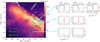Fig. 1

Overview of the Orion Bar. The (0″, 0″) position corresponds to α₂₀₀₀ = 05^h 35^m 20.1^s ; δ₂₀₀₀ = -05°25′07.0″. Left panel: integrated line intensity maps in the ¹³CO J = 3–2 (color scale) and SO 8₉–7₈ emission (gray contours; from 6 to 23.5 K km s⁻¹ in steps of 2.5 K km s⁻¹) obtained with the IRAM 30 m telescope at 8″ resolution. The white dotted contours delineate the position of the H₂ dissociation front as traced by the infrared H₂ v = 1–0 S(1) line (from 1.5 to 4.0 × 10⁻⁴ erg s⁻¹ cm⁻² sr⁻¹ in steps of 0.5 × 10⁻⁴ erg s⁻¹ cm⁻² sr⁻¹; from Walmsley et al. 2000). The black-dashed rectangle shows the smaller FoV imaged with ALMA (Fig. 3). The DF position has been observed with SOFIA, IRAM 30 m, and Herschel. Cyan circles represent the ~15″ beam at 168 GHz. Right panel: H₂S lines lines detected toward three positions of the Orion Bar.

2.2 Observations of H₂S isotopologues and H₃ S⁺

We observed the Orion Bar with the IRAM 30 m telescope at Pico Veleta (Spain). We used the EMIR receivers in combination with the Fast Fourier Transform Spectrometer (FTS) backends at 200 kHz resolution (~0.4, ~0.3, and ~0.2 km s⁻¹ at ~168, ~217, and ~293 GHz, respectively). These observations are part of a complete line survey covering the frequency range 80–360 GHz (Cuadrado et al. 2015, 2016, 2017, 2019) and include deep integrations at 168 GHz toward three positions of the PDR located at a distance of 14″, 40″, and 65″ from the IF (see Fig. 1). Their offsets with respect to the IF position at α₂₀₀₀ = 05^h 35^m 20.1^s, δ₂₀₀₀ = -05°25′07.0″ are (+10″, −10″), (+30″, −30″’), and (+35″, −55″). The first position is the DF.

We carried out these observations in the position switching mode taking a distant reference position at (−600″, 0″). The half power beam width (HPBW) at ~168, ~217, and ~293 GHz is ~15″, ~11″, and ~8″, respectively. The latest observations (those at 168 GHz) were performed in March 2020. The data were first calibrated in the antenna temperature scale $T_{A}^{*}$ $T^{*}_{\textrm{A}}$ and then converted to the main beam temperature scale, T_mb, using T_mb = $T_{A}^{*} / η_{mb}$ $T^{*}_{\textrm{A}}/ \eta_{\textrm{mb}}$ , where η_mb is the antenna efficiency (η_mb = 0.74 at ~168 GHz). We reduced andanalyzed the data using the GILDAS software as described in Cuadrado et al. (2015). The typical rms noise of the spectra is ~3.5, 5.3, and 7.8 mK per velocity channel at ~168, ~217, and ~293 GHz, respectively.Figures 1 and 2 show the detection of o-H₂S 1_1,0 −1_0,1 (168.7 GHz), p-H₂S 2_2,0 −2_1,1 (216.7 GHz), and o-H₂ ³⁴ S 1_1,0 −1_0,1 lines (167.9 GHz) (see Table E.1 for the line parameters), as well as several o-H₂ ³³ S 1_1,0 −1_0,1 hyperfine lines (168.3 GHz).

We complemented our dataset with higher frequency H₂ S lines detected by the Herschel Space Observatory (Nagy et al. 2017) toward the “CO⁺ peak” position (Stoerzer et al. 1995), which is located at only ~4″ from our DF position (i.e., within the HPBW of these observations). These observations were carried out with the HIFI receiver (de Graauw et al. 2010) at a spectral-resolution of 1.1 MHz (0.7 km s⁻¹ at 500 GHz). HIFI’s HPBW range from ~42″ to ~20″ in the 500–1000 GHz window (Roelfsema et al. 2012). The list of additional hydrogen sulfide lines detected by Herschel includes the o-H₂S 2_2,1 −2_1,2 (505.5 GHz), 2_1,2 −1_0,1 (736.0 GHz), and 3_0,3 −2_1,2 (993.1 GHz), as well as the p-H₂S 2_0,2 −1_1,1 (687.3 GHz) line. We used the line intensities, in the T_mb scale, shown in Table A.1 of Nagy et al. (2017).

In order to get a global view of the Orion Bar, we also obtained 2.5′ × 2.5′ maps of the region observed by us with the IRAM 30 m telescope using the 330 GHz EMIR receiver and the FTS backend at 200 kHz spectral-resolution (~0.2 km s⁻¹). On-the-fly (OTF) scans were obtained along and perpendicular to the Bar. The resulting spectra were gridded to a data cube through convolution with a Gaussian kernel providing a final resolution of ~8″. The total integration time was ~6 h. The achieved rms noise is ~1 K per resolution channel. Figure 1 shows the spatial distribution of the ¹³ CO J = 3–2 (330.5 GHz) and SO 8₉-7₈ (346.5 GHz) integrated line intensities.

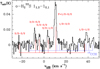Fig. 2

Detection of H₂ ³³ S (at ~168.3 GHz) toward the DF position of the Orion Bar. Red lines indicate hyperfine components. Blue lines show interloping lines from ¹³CCH. The length of each line is proportional to the transition line strength (taken from the Cologne Database for Molecular Spectroscopy, CDMS; Endres et al. 2016).

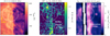Fig. 3

ALMA 1″-resolution images zooming into the edge of the Orion Bar in ¹²CO 3–2 (left panel, Goicoechea et al. 2016) and SH⁺ 1₀ –0₁ F = 1/2–3/2 line (middle panel, integrated line intensity). The right panel shows the H₂ v = 1–0 S(1) line (Walmsley et al. 2000). We rotated these images (all showing the same FoV) with respect to Fig. 1 to bring the FUV illuminating direction in the horizontal direction (from the right). The circle shows the DF position targeted with SOFIA in SH (20″ beam) and with the IRAM 30 m telescope in H₂S and H₃S⁺.

2.3 ALMA imaging of Orion Bar edge in SH⁺ emission

We carried out mosaics of a small field of the Orion Bar using twenty-seven ALMA 12 m antennas in band 7 (at ~346 GHz). These unpublished observations belong to project 2012.1.00352.S (PI: J. R. Goicoechea) and consisted of a 27-pointing mosaic centered at α(2000) = 5^h35^m20.6^s; δ(2000) = −05°25′20″. The total field-of-view (FoV) is 58″ × 52″ (shown in Fig. 1). The two hyperfine line components of the SH⁺ N_J = 1₀−0₁ transition were observed with correlators providing ~500 kHz resolution (0.4 km s⁻¹) over a 937.5 MHz bandwidth. The total observation time with the ALMA 12 m array was ~2h. In order to recover the large-scale extended emission filtered out by the interferometer, we used deep and fully sampled single-dish maps, obtained with the total-power (TP) antennas at 19″ resolution, as zero- and short-spacings. Data calibration procedures and image synthesis steps are described in Goicoechea et al. (2016). The synthesized beam is ~1″. This is a factor of ~4 better than previous interferometric SH⁺ observations (Goicoechea et al. 2017). Figure 3 shows the resulting image of the SH⁺ 1₀ − 0₁ F = 1/2–3/2 hyperfine emission line at 345.944 GHz. We rotated this image 37.5° clockwise to bring the FUV illumination in the horizontal direction. The typical rms noise of the final cube is ~ 80 mK per velocity channel and 1″-beam. As expected from their Einstein coefficients, the other F = 1/2–1/2 hyperfine line component at 345.858 GHz is a factor of ~2 fainter (see Table E.2) and the resulting image has low signal-to-noise (S/N).

We complemented the SH⁺ dataset with the higher frequency lines observed by HIFI (Nagy et al. 2013, 2017) at ~526 and ~683 GHz (upper limit). These pointed observations have HPBWs of ~41″ and ~32″ respectively, thus they do not spatially resolve the SH⁺ emission. To determine their beam coupling factors (f_b), we smoothed the bigger 4″-resolution ACA + TP SH⁺ image shown in Goicoechea et al. (2017) to the different HIFI’s HPBWs. We obtain f_b ≃ 0.4 at ~526 GHz and f_b ≃ 0.6 at ~683 GHz. The corrected intensities are computed as W_corr = W_HIFI / f_b. These correction factors are only a factor of ≲2 lower than simply assuming uniform SH⁺ emission from a 10″ width filament.

2.4 SOFIA/GREAT search for SH emission

We finally used the GREAT receiver (Heyminck et al. 2012) on board the Stratospheric Observatory For Infrared Astronomy (SOFIA; Young et al. 2012) to search for the lowest-energy rotational lines of SH (² Π_3∕2 J = 3/2–1/2) at 1382.910 and 1383.241 GHz (e.g., Klisch et al. 1996; Martin-Drumel et al. 2012). These lines lie in a frequency gap that Herschel/HIFI could not observe from space. These SOFIA observations belong to project 07_ 0115 (PI: J. R. Goicoechea). The SH lines were searched on the lower side band of 4GREAT band 3. We employed the 4GREAT/HFA frontends and 4GFFT spectrometers as backends. The HPBW of SOFIA at 1.3 THz is ~20″, thus comparable with IRAM 30 m/EMIR and Herschel/HIFI observations. We also employed the total power mode with a reference position at (−600″,0″). The originalplan was to observe during two flights in November 2019 but due to bad weather conditions, only ~70 min of observationswere carried out in a single flight.

After calibration, data reduction included: removal of a first order spectral baseline, dropping scans with problematic receiver response, rms weighted average of the spectral scans, and calibration to T_mb intensity scale (η_mb = 0.71). The final spectrum, smoothed to a velocity-resolution of 1 km s⁻¹ has a rms noise of ~50 mK (shown in Fig. 4). Two emission peaks are seen at the frequencies of the Λ-doublet lines. Unfortunately, the achieved rms is not enough to assure the unambiguous detection of each component of the doublet. Although the stacked spectrum does display a single line (suggesting a tentative detection) the resulting line-width (Δv ≃ 7 km s⁻¹) is a factor of ~3 broader than expected in the Orion Bar (see Table E.3). Hence, this spectrum provides stringent upper limits to the SH column density but deeper integrations would be needed to confirm the detection.

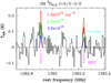Fig. 4

Search for the SH ² Π_3∕2 J = 5/2–3/2 doublet (at ~1383 GHz) toward the DF position with SOFIA/GREAT. Vertical magenta lines indicate the position of hyperfine splittings taken from CDMS.

3 Observational results

3.1 H₂³² S, H₂³⁴ S, and H₂³³ S across the PDR

Figure 1 shows an expanded view of the Orion Bar in the ¹³ CO (J = 3–2) emission. FUV radiation from the Trapezium stars comes from the upper-right corner of the image. The FUV radiation field is attenuated in the direction perpendicular to the Bar. The infrared H₂ v = 1–0 S(1) line emission (white contours) delineates the position of the H-to-H₂ transition, the DF. Many molecular species, such as SO, specifically emit from deeper inside the PDR where the flux of FUV photons has considerably decreased. In contrast, H₂ S, and even its isotopologueH $_{2}^{34}$ $_{2}^{34}$ S, show bright 1_1,0 –1_0,1 line emission toward the DF (right panels in Fig. 1; see also Jansen et al. 1995). Rotationally excited H₂ S lines have been also detected toward this position (Nagy et al. 2017), implying the presence of warm H₂ S close to the irradiated cloud surface (i.e., at relatively low extinctions). The presence of moderately large H₂ S column densities in the PDR is also demonstrated by the unexpected detection of the rare isotopologue H $_{2}^{33}$ $_{2}^{33}$ S toward the DF (at the correct LSR velocity of the PDR: v_LSR ≃ 10.5 km s⁻¹). Figure 2 shows the H $_{2}^{33}$ $_{2}^{33}$ S 1_1,0 –1_0,1 line and its hyperfine splittings (produced by the ³³S nuclear spin). To our knowledge, H $_{2}^{33}$ $_{2}^{33}$ S lines had only been reported toward the hot cores in Sgr B2 and Orion KL before (Crockett et al. 2014).

The observed o-H₂S/o–H $_{2}^{34}$ $_{2}^{34}$ S 1_1,0 -1_0,1 line intensity ratio toward the DF is 15 ± 2, below the solar isotopic ratio of ³² S/³⁴S = 23 (e.g., Anders & Grevesse 1989). The observed ratio thus implies optically thick o-H₂S line emission at ~168 GHz. However, the observed o-H $_{2}^{34}$ $_{2}^{34}$ S/o-H $_{2}^{33}$ $_{2}^{33}$ S 1_1,0 –1_0,1 intensity ratio is 6 ± 1, thus compatible with the solar isotopic ratio (³⁴ S/³³S = 5.5) and with H $_{2}^{34}$ $_{2}^{34}$ S and H $_{2}^{33}$ $_{2}^{33}$ S optically thin emission.

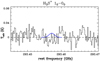Fig. 5

Search for H₃S⁺ toward the Orion Bar with the IRAM 30 m telescope. The blue curve shows the expected position of the line.

3.2 SH⁺ emission from the PDR edge

Figure 3 zooms into a small field of the Bar edge. The ALMA image of the CO J = 3–2 line peak temperature was first presented by Goicoechea et al. (2016). Because the CO J = 3–2 emission is nearly thermalized and optically thick from the DF to the molecular cloud interior, the line peak temperature scale (T_peak) is a good proxy of the gas temperature (T_k ≃T_ex ≃T_peak). The CO image implies small temperature variations around T_k ≃ 200 K. The middle panel in Fig. 3 shows the ALMA image of the SH⁺ N_J = 1₀–0₁ F = 1/2–3/2 hyperfine line at 345.944 GHz. Compared to CO, the SH⁺ emission follows the edge of the molecular PDR, akin to a filament of ~10″ width (for the spatial distribution of other molecular ions, see, Goicoechea et al. 2017). The SH⁺ emission shows localized small-scale emission peaks (density or column density enhancements) that match, or are very close to, the vibrationally excited H₂ (v = 1–0) emission (Fig. 3). We note that while some H₂ (v = 1–0) emission peaks likely coincide with gas density enhancements (e.g., Burton et al. 1990), the region also shows extended emission from FUV-pumped H₂ (v = 2–1) (van der Werf et al. 1996) that does not necessarily coincide with the H₂ (v = 1–0) emission peaks.

3.3 Search for SH, H₃ S⁺, and H₂ S ν₂ = 1 emission

We used SOFIA/GREAT to search for SH ² Π_3∕2 J = 5/2–3/2 lines toward the DF (Fig. 4). This would have been the first time that interstellar SH rotational lines were seen in emission. Unfortunately, the achieved rms of the observation does not allow a definitive confirmation of these lines, so here we will only discuss upper limitsto the SH column density. The red, green, and blue curves in Fig. 4 show radiative transfer models for n_H = 10⁶ cm⁻³, T_k = 200 K, and different SH column densities (see Sect. 4 for more details).

Our IRAM 30 m observations toward the DF neither resulted in a detection of H₃ S⁺, a key gas-phase precursor of H₂S. The ~293.4 GHz spectrum around the targeted H₃ S⁺ 1₀–0₀ line is shown in Fig. 5. Again, the achieved low rms allows us to provide a sensitive upper limit to the H₃ S⁺ column density. This results in N(H₃S⁺) = (5.5–7.5) × 10¹⁰ cm⁻² (5σ) assuming an excitation temperature range T_ex = 10–30 K and extended emission. Given the bright H₂S emission close to the edge of the Orion Bar, and because H₂S formation at the DF might be driven by very exoergic processes, we also searched for the 1_1,0 –1_0,1 line of vibrationally excited H₂S (in the bending mode ν₂). The frequency of this line lies at ~181.4 GHz (Azzam et al. 2013), thus at the end of our 2 mm-band observations of the DF (rms ≃ 16 mK). However, we do not detect this line either.

4 Coupled nonlocal excitation and chemistry

In this section we study the rotational excitation of the observed S-bearing hydrides³. We determine the SH⁺, SH (upper limit), and H₂S column densities in the Orion Bar, and the “average” gas physical conditions in the sense that we search for the combination of single T_k, n_H, and N that better reproduces the observed line intensities (so-called “single-slab” approach). In Sect. 6 we expand these excitation models to multi-slab calculations that take into account the expected steep gradients in a PDR.

In the ISM, rotationally excited levels are typically populated by inelastic collisions. However, the lifetime of very reactive molecules can be so short that the details of their formation and destruction need to be taken into account when determining how these levels are actually populated (Black 1998). Reactive collisions (collisions that lead to a reaction and thus to molecule destruction)influence the excitation of these species when their timescales become comparable to those of nonreactive collisions. The lifetimeof reactive molecular ions observed in PDRs (e.g., Fuente et al. 2003; Nagy et al. 2013; van der Tak et al. 2013; Goicoechea et al. 2017, 2019) can be so short that they do not get thermalized by nonreactive collisions or by absorption of the background radiation field (Black 1998). In these cases, a proper treatment of the molecule excitation requires including chemical formation and destruction rates in the statistical equilibrium equations (dn_i / dt = 0) that determine the level populations: $\begin{array}{l} \sum_{j > i} n_{j} A_{j i} + \sum_{j \neq i} n_{i} (B_{j i} {\bar{J}}_{j i} + C_{j i}) + F_{i} \\ = n_{i} (\sum_{j < i} A_{i j} + \sum_{j \neq i} (B_{i j} {\bar{J}}_{i j} + C_{i j}) + D_{i}), \end{array}$ $\begin{eqnarray*} && {\hspace*{-6pt}} \sum_{j>i} n_j\,A_{ji} + \sum_{j \neq i} n_i \left(B_{ji}\,\bar{J}_{ji} + C_{ji} \right) + F_i \\ && \qquad =\, n_i \left(\sum_{j<i} A_{ij} + \sum_{j \neq i} \left(B_{ij}\,\bar{J}_{ij} + C_{ij} \right) \,+\, D_i \right), \end{eqnarray*}$

where n_i [cm ⁻³] is the population of rotational level i, A_ij and B_ij are the Einstein coefficients for spontaneous and induced emission, C_ij [s ⁻¹ ] is the rate of inelastic collisions⁴ (C_ij = ∑_kγ_{ij, k} n_k, where γ_{ij, k}(T) [cm ³s⁻¹] are the collisional rate coefficients and k stands for H₂, H, and e⁻), and ${\bar{J}}_{i j}$ $\bar{J}_{ij}$ is the mean intensity of the total radiation field over the line profile. In these equations, n_i D_i is the destruction rate per unit volume of the molecule in level i, and F_i its formation rate per unit volume (both in cm⁻³s⁻¹). When state-to-state formation rates are not available, and assuming that the destruction rate is the same in every level (D_i = D), one can use the total destruction rate D [s⁻¹] (= ∑_kn_k k_k(T) + photodestruction rate, where k_k [cm ³s⁻¹] is the state-averaged rate of the two-body chemical reaction with species k) and consider that the level populations of the nascent molecule follow a Boltzmann distribution at an effective formation temperature T_form: $F_{i} = F g_{i} e^{- E_{i} / k T_{form}} / Q (T_{form}) .$ $\begin{equation*} F_i\,{=}\,F\, g_i \, e^{-E_i/kT_{\textrm{form}}} \,/\, Q(T_{\textrm{form}}). \end{equation*}$ (7)

In this formalism, F [cm ⁻³ s⁻¹] is the state-averaged formation rate per unit volume, g_i the degeneracy of level i, and Q(T_form) is the partition function at T_form (van der Tak et al. 2007).

This “formation pumping” formalism has been previously implemented in large velocity gradient codes to treat, for example, the local excitation of the very reactive ion CH⁺ (Nagy et al. 2013; Godard & Cernicharo 2013; Zanchet et al. 2013b; Faure et al. 2017). However, interstellar clouds are inhomogeneous and gas velocity gradients are typically modest at small spatial scales. This means that line photons can be absorbed and reemitted several times before leaving the cloud. Here we implemented this formalism in a Monte Carlo code that explicitly models the nonlocal behavior of the excitation and radiative transfer problem (see Appendix of Goicoechea et al. 2006).

Although radiative pumping by dust continuum photons does not generally dominate in PDRs, for completeness we also included radiative excitation by a modified blackbody at a dust temperature of ~50 K and a dust opacity τ_λ = 0.03 (150/λ[μm])^1.6 (which reproduces the observed intensity and wavelength dependence of the dust emission in the Bar; Arab et al. 2012). The molecular gas fraction, f(H₂) = 2n(H₂)/n_H, is set to 2/3, where n_H = n(H) + 2n(H₂) is the total density of H nuclei. This choice is appropriate for the dissociation front and implies n(H₂) = n(H). As most electrons in the DF come from the ionization of carbon atoms, the electron density n_e is set to n_e ≃n(C⁺) = 1.4 × 10⁻⁴ n_H (e.g., Cuadrado et al. 2019). For the inelastic collisions with o-H₂ and p-H₂, we assumed that the H₂ ortho-to-para (OTP) ratio is thermalized to the gas temperature.

4.1 SH⁺ excitation and column density

We start by assuming that the main destruction pathway of SH⁺ are reactions with H atoms and recombinations with electrons (see Sect. 6.1). Hence, the SH⁺ destruction rate is D ≃n_e k_e(T) + n(H) k_H(T) (see Table 1 for the relevant chemical destruction rates). For T_k = T_e = 200 K and n_H = 10⁶ cm⁻³ (e.g., Goicoechea et al. 2016) this implies D ≃ 10⁻⁴ s⁻¹ (i.e., the lifetime of an SH⁺ molecule in the Bar is less than 3 h). At these temperatures and densities, D is about ten times smaller than the rate of radiative and inelastic collisional transitions that depopulate the lowest-energy rotational levels of SH⁺. Hence, formation pumping does not significantly alter the excitation of the observed SH⁺ lines, but it does influence the population of higher-energy levels. Formation pumping effects have been readily seen in CH⁺ because this species is more reactive⁵ and its rotationally excited levels lie at higher-energy (i.e., their inelastic collision pumping rates are slower, e.g., Zanchet et al. 2013b)

Figure 6 shows results of several models: without formation pumping (dotted curves for model “F = D = 0”), adding formation pumping with SH⁺ destruction by H and e⁻ (continuous curves for model “F, D”), and using a factor of ten higher SH⁺ destruction rates (simulating a dominant role of SH⁺ photodissociation or destruction by reactions with vibrationally excited H₂ ; dashed curves for model “F, D × 10”). Since the formation of SH⁺ is driven by reaction (1) when H₂ molecules are in v ≥ 2, here we adopted T_form ≃E(v = 2, J = 0) / k− 9860 K ≈ 2000 K. Because these are constant column density N(SH⁺) excitation and radiative transfer models, we used a normalized formation rate F = ∑ F_i that assumes steady-state SH⁺ abundances consistent with the varying gas density in each model. That is, F = ∑ F_i = x(SH⁺) n_H D [cm ⁻³s⁻¹], where x refers to the abundance with respect to H nuclei.

The detected SH⁺ rotational lines connect the fine-structure levels N_J = 1₀–0₁ (345 GHz) and 1₂ –0₁ (526 GHz). Upper limits also exist for the 1₁ -0₁ (683 GHz) lines. SH⁺ critical densities (n_cr = A_ij / γ_ij) for inelastic collisions with H or H₂ are of the same order and equal to several 10⁶ cm⁻³. As for many molecular ions (e.g., Desrousseaux et al. 2021), SH⁺–H₂ (and SH⁺–H) inelastic collisional rate coefficients⁴ are large (γ_ij ≳ 10⁻¹⁰ cm³ s⁻¹). Thus, collisions with H (at low A_V) and H₂ (at higher A_V) generally dominate over collisions with electrons (γ_ij of a few 10⁻⁷ cm³ s⁻¹). At low densities (meaning n_H <n_cr) formation pumping increases the population of the higher-energy levels (and their T_ex), but there are only minor effects in the low-energy submillimeter lines. At high densities, n_H > 10⁷ cm⁻³, formation pumping with T_form = 2000 K produces lower intensities in these lines because the lowest-energy levels (E_u ∕k <T_k <T_form) are less populated.

The best fit to the observed lines in model F, D is for N(SH⁺) ≃ 1.1 × 10¹³ cm⁻³, n_H ≃ 3 × 10⁵ cm⁻³, and T_k ≃ 200 K. This is shown by the vertical dotted line in Fig. 6. This model is consistent with the upper limit intensity of the 683 GHz line (Nagy et al. 2013). In this comparison, and following the morphology of the SH⁺ emission revealed by ALMA (Fig. 3), we corrected the line intensities of the SH⁺ lines detected by Herschel/HIFI with the beam coupling factors discussed in Sect. 2.3, The observed 1₂ –0₁/1₀–0₁ line ratio (R = W(526.048)/W(345.944) ≃ 2) is sensitive to the gas density. In these models, R is 1.1 for n_H = 10⁵ cm⁻³ and 3.0 for n_H = 10⁶ cm⁻³. We note that n_H could be lower if SH⁺ formation/destruction rates were faster, as in the F, D × 10 model. This could happen if SH⁺ photodissociation or destruction reactions with H₂ (v ≥ 2) were faster than reactions of SH⁺ with H atoms or with electrons. In Sect. 6 we show that this is not the case.

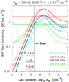Fig. 6

Non-LTE excitation models of SH⁺. The horizontal lines mark the observed line intensities in the Orion Bar. Dotted curves are for a standard model (F = D = 0). Continuous curves are for a model that includes chemical destruction by H atoms and e⁻ (model F, D). Dashed lines are for a model in which destruction rates are multiplied by ten (model F, D × 10). The verticalblack line marks the best model.

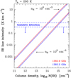Fig. 7

Non-LTE excitation models of SH emission lines targeted with SOFIA/GREAT. Horizontal dashed lines refer to observational limits, assuming extended emission (lower intensities) and for a 10″ width emission filament at the PDR surface (higher intensities).

4.2 SH excitation and column density

SH is a ²Π open-shell radical with fine-structure, Λ-doubling, and hyperfine splittings (e.g., Martin-Drumel et al. 2012). However, the frequency separation of the SH ² Π_3∕2 J = 5/2–3/2 hyperfine components is too small to be spectrally resolved in observations of the Orion Bar (see Fig. 4).The available rate coefficients for inelastic collisions of SH with helium atoms do not resolve the hyperfine splittings. Hence, we first determined line frequencies, level degeneracies, and Einstein coefficients of an SH molecule without hyperfine structure. To do this, we took the complete set of hyperfine levels tabulated in CDMS. Lacking specific inelastic collision rate coefficients, we scaled the available SH– He rates of Kłos et al. (2009) by the square root of the reduced mass ratios and estimated the SH– H and SH– H₂ collisional rates.

The scaled rate coefficients are about an order of magnitude smaller than those of SH⁺. However, the chemical destruction rate of SH at the PDR edge (reactions with H, photodissociation, and photoionization, see Sect. 6.1) is also slower (we take the rates of SH–H reactive collisions from Zanchet et al. 2019). We determine D ≃ 3 × 10⁻⁶ s⁻¹ for n_H = 10⁶ cm⁻³, T_k = 200 K, and A_V ≃ 0.7 mag. Models in Fig. 7 include these chemical rates for T_form = T_k (a lower limit to the unknown formation temperature). Formation pumping enhances the intensity of the ² Π_3∕2 J = 5/2–3/2 ground-state lines by a few percent only.

To estimate the SH column density in the Orion Bar we compare with the upper limit intensities of the SH lines targeted by SOFIA. If SH and SH⁺ arise from roughly the same gas at similar physical conditions (n_H ≃ 10⁶ cm⁻³ and T_k ≃ 200 K) the best model column density is for N(SH) ≤ (0.6–1.6) × 10¹⁴ cm⁻². If densities were lower, around n_H ≃ 10⁵ cm⁻³, the upper limit N(SH) column densities will be a factor ten higher.

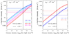Fig. 8

Non-LTE excitation models for o-H₂S and p-H₂S. Thin horizontal lines show the observed intensities assuming either extended emission (lower limit) or emission that fills the 15″ beam at168.7 GHz. The vertical line marks the best model, resulting in an OTP ratio of 2.9 ± 0.3.

4.3 H₂S excitation and column density

H₂ S has a X² A ground electronic state and two nuclear spin symmetries that we treat separately, o-H₂S and p-H₂S. Previous studies of the H₂S line excitation have used collisional rates coefficients scaled from those of the H₂ O – H₂ system. Dagdigian (2020) recently carried out specific calculations of the cross sections of o-H₂S and p-H₂S inelastic collisions with o–H₂ and p-H₂ at different temperatures. The behavior of the new and the scaled rates is different and it depends on the H₂ OTP ratio (e.g., on gas temperature) because the collisional cross sections are different for o-H₂–H₂S and p-H₂–H₂S systems. At the warm temperatures of the PDR, collisions with o-H₂ dominate, resulting in rate coefficients for the ~168 GHz o-H₂S line that are a factor up to ~2.5 smaller than those scaled from H₂ O–H₂.

H₂S is not a reactive molecule. At the edge of the PDR its destruction is driven by photodissociation. We determine that the radiative and collisional pumping rates are typically a factor of ~100 higher than D ≈ 2 × 10⁻⁶ s⁻¹ (for n_H = 10⁶ cm⁻³, T_k = 200 K, G₀ ≃10⁴, and A_V ≃ 0.7 mag). Figure 8 shows non-LTE o-H₂S and p-H₂S excitation and radiative transfer models. As H₂S may have its abundance peak deeper inside the PDR and display more extended emission than SH⁺ (e.g., Sternberg & Dalgarno 1995), we show results for T_k = 200 and 100 K. When comparing with the observed line intensities, we considered either emission that fills all beams, or a correction that assumes that the H₂S emission only fills the15″ beam of the IRAM 30 m telescope at 168 GHz. The vertical dotted lines in Fig. 8 show the best model, N(H₂S) = N(o-H₂S)+N(p-H₂S) = 2.5 × 10¹⁴ cm⁻², with an OTP ratio of 2.9 ± 0.3, thus consistent with the high-temperature statistical ratio of 3/1 (see discussion at the end of Sect. 6.4). Models with lower densities, n_H ≃ 10⁵ cm⁻³, show worse agreement, and would translate into even higher N(H₂S) of ≳ 10¹⁵ cm⁻². In either case, these calculations imply large columns of warm H₂ S toward the PDR. They result in a limit to the SH to H₂S column density ratio of ≤0.2–0.6. This upper limit is already lower than the N(SH)/N(H₂S) = 1.1–3.0 ratios observed in diffuse clouds (Neufeld et al. 2015). This difference suggests an enhanced H₂ S formation mechanism in FUV-illuminated dense gas.

5 New results on sulfur-hydride reactions

In this section we summarize the ab initio quantum calculations we carried out to determine the vibrationally-state-dependent rates of gas-phase reactions of H₂ (v > 0) with several S-bearing species. We recall that all hydrogen abstraction reactions, $S^{+} \to_{(1)}^{+ H_{2}} {SH}^{+} \to_{(2)}^{+ H_{2}} H_{2} S^{+} \to_{(3)}^{+ H_{2}} H_{3} S^{+}, S \to_{(4)}^{+ H_{2}} SH, 0.1 c m$ $\textrm{S}^+ \xrightarrow[(1)]{{{+{\textrm{H}_2}}}} \textrm{SH}^+ \xrightarrow[(2)]{{+{\textrm{H}_2}}} {\textrm{H}_2S^+} \xrightarrow[(3)]{{+{\textrm{H}_2}}} {\textrm{H}_3\textrm{S}^+,}\hspace{1cm}\textrm{S} \xrightarrow[(4)]{{{+{\textrm{H}_2}}}} \textrm{SH,}\vspace{0.1cm}$ are very endoergic for H₂ (v = 0), with endothermicities in Kelvin units that are significantly higher than T_k even in PDRs. This is markedly different to O⁺ chemistry, for which all hydrogen abstraction reactions leading to H₃ O⁺ are exothermic and fast (Gerin et al. 2010; Neufeld et al. 2010; Hollenbach et al. 2012).

The endothermicity of reactions involving H_n S⁺ ions decreases as the number of hydrogen atoms increases. The potential energy surfaces (PES) of these reactions possess shallow wells at the entrance and products channels (shown in Fig. 9). In addition, these PESs show saddle points between the energy walls of reactants and products whose heights increase with the number of H atoms. For reaction (2), the saddle point has an energy of 0.6 eV (≃7000 K) and is slightly below the energy of the products. However, for reaction (3), the saddle point is above the energy of the products and is a reaction barrier. These saddle points act as a bottleneck in the gas-phase hydrogenation of S⁺.

If one considers the state dependent reactivity of vibrationally excited H₂, the formation of SH⁺ through reaction (1) becomes exoergic⁶ when v ≥ 2 (Zanchet et al. 2019). The detection of bright H₂S emission in the Orion Bar (Figs. 1 and 4) might suggest that subsequent hydrogen abstraction reactions with H₂ (v ≥ 2) proceed as well. Motivated by these findings, and before carrying out any PDR model, we studied reaction (2) and the reverse process in detail. This required to build a full dimensional quantum PES of the H₃ S⁺ (X¹A₁) system (see Appendix A).

In addition, we studied reaction (4) (and its reverse) through quantum calculations. Details of these ab initio calculations and of the resulting reactive cross sections are given in Appendix B. Table 1 summarizes the updated reaction rate coefficients that we will include later in our PDR models.

The H₂ S⁺ formation rate through reaction (2) with H₂ (v = 0) is very slow. For H₂ (v = 1), the rate constant increases at ≈500 K, corresponding to the opening of the H₂ S⁺ + H threshold. For H₂ (v = 2) and H₂ (v = 3), the reactionrate is much faster, close to the Langevin limit (see Appendix A.2). However, our estimated vibrational-state specific rates for SH formation through reaction (4) (S + H₂) are considerably smaller than for reactions (1) and (2), and show an energy barrier even for H₂ (v = 2) and H₂ (v = 3). We anticipate that this reaction is not a relevant formation route for SH.

In FUV-illuminated environments, collisions with H atoms are very important because they compete with electron recombinations in destroying molecular ions, and also they contribute to their excitation. An important result of our calculations is that the destruction rate of H₂ S⁺ (SH⁺) in reactions with H atoms are a factor of ≥3.5 (≥1.7) faster (at T_k ≤ 200 K) than those previously used in astrochemical models (Millar et al. 1986). Conversely, we find that destruction of SH in reactions with H atoms (Appendix B) is slower than previously assumed.

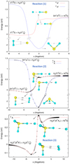Fig. 9

Minimum energy paths for reactions (1), (2), and (3). Points correspond to RCCSD(T)-F12a calculations and lines to fits (Appendix A). The reaction coordinate, s, is defined independently for each path. The geometries of each species at s = 0 are different.

Table 1

Relevant rate coefficients from a fit of the Arrhenius-like form k (T) = 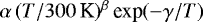$α {(T / 300 K)}^{β} exp (- γ / T)$ $\alpha\,(T/300\,\textrm{K})^{\beta} \,\textrm{exp}(-\gamma/T)$ to the calculated reaction rates.

6 PDR models of S-bearing hydrides

We now investigate the chemistry of S-bearing hydrides and the effect of the new reaction rates in PDR models adapted to the Orion Bar conditions. In this analysis we used version 1.5.4. of the Meudon PDR code (Le Petit et al. 2006; Bron et al. 2014). Following our previous studies, we model the Orion Bar as a stationary PDR at constant thermal-pressure (i.e., with density and temperature gradients). When compared to time-dependent hydrodynamic PDR models (e.g., Hosokawa & Inutsuka 2006; Bron et al. 2018; Kirsanova & Wiebe 2019), stationary isobaric models seem a good description of the most exposed and compressed gas layers of the PDR, from A_V ≈ 0.5 to ≈ 5 mag (Goicoechea et al. 2016; Joblin et al. 2018).

In our models, the FUV radiation field incident at the PDR edge is G₀ = 2 × 10⁴ (e.g., Marconi et al. 1998). We adopted an extinction to color-index ratio, R_V = A_V/E_B−V, of 5.5 (Joblin et al. 2018), consistent with the flatter extinction curve observed in Orion (Lee 1968; Cardelli et al. 1989). This choice implies slightly more penetration of FUV radiation into the cloud (e.g., Goicoechea & Le Bourlot 2007). The main input parameters and elemental abundances of these PDR models are summarized in Table 2. Figure 10 shows the resulting H₂, H, and electron density profiles, as well as the T_k and T_d gradients.

Our chemical network is that of the Meudon code updated with the new reaction rates listed in Table 1. This network includes updated photoreaction rates from Heays et al. (2017). To increase the accuracy of our abundance predictions, we included the explicit integration of wavelength-dependent SH, SH⁺, and H₂ S photodissociation cross sections (σ_diss), as well as SH and H₂S photoionization cross sections (σ_ion). These cross sections are shown in Fig. C.1. The integration is performed over the specific FUV radiation field at each position of the PDR. In particular, we took σ_ion(SH) from Hrodmarsson et al. (2019) and σ_diss(H₂S) from Zhou et al. (2020), both determined in laboratory experiments. Figure 11 summarizes the relevant chemical network that leads to the formation of S-bearing hydrides and that we discuss in the following sections.

Table 2

Main parameters used in the PDR models of the Orion Bar.

6.1 Pure gas-phase PDR model results

Figure 12 shows results of the “new gas-phase” model using the reaction rates in Table 1. The continuous curves display the predicted fractional abundance profiles as a function of cloud depth in magnitudes of visual extinction (A_V). The dashed curves are for a model that uses the standard thermal rates previously adopted in the literature (see, e.g., Neufeld et al. 2015). As noted by Zanchet et al. (2013a, 2019), the inclusion of H₂ (v ≥ 2) state-dependent quantum rates for reaction (1) enhances the formation of SH⁺ in a narrow layer at the edge of the PDR (A_V ≃ 0 to 2 mag). This agrees with the morphology of the SH⁺ emission revealed by ALMA images (Fig. 3). For H₂ (v = 2), the reaction rate enhancement with respect to the thermal rate Δk = k₂(T)∕k₀(T) (see discussion by Agúndez et al. 2010) is about 4 × 10⁸ at T_k = 500 K (Millar et al. 1986). Indeed, when the fractional abundance of H₂ (v = 2) with respect to H₂ (v = 0), defined as f₂ = n (H₂ v = 2)/n (H₂ v = 0), exceeds a few times 10⁻⁹, meaning Δk ⋅f₂ > 1, reaction (1) with H₂ (v ≥ 2) dominates SH⁺ formation. This reaction enhancement takes place only at the edge of the PDR, where FUV-pumped H₂ (v ≥ 2) molecules are abundant enough (gray dashed curves in Fig. 12) and drive the formation of SH⁺. The resulting SH⁺ column density increases by an order of magnitude compared to models that use the thermal rate.

In this isobaric model, the SH⁺ abundance peak occurs at A_V ≃ 0.7 mag, where the gas density has increased from n_H ≃ 6 × 10⁴ cm⁻³ at the PDR edge (the IF) to ~5 × 10⁵ cm⁻³ (at the DF). At this point, SH⁺ destruction is dominated by recombination with electrons and by reactive collisions with H atoms. This implies D(SH⁺) [s⁻¹ ] ~n_e k_e ≃ n_H k_H ≫n(H₂ v ≥ 2) k₂, as we assumed in the single-slab SH⁺ excitation models (Sect. 4.1). Therefore, only a small fraction of SH⁺ molecules further react with H₂ (v ≥ 2) to form H₂ S⁺. The resulting low H₂ S⁺ abundances limit the formation of abundant SH from dissociative recombinations of H₂ S⁺ (recall that we estimated that reaction S + H₂ (v ≥2) → SH + H is very slow). The SH abundance peak is shifted deeper inside the cloud, at about A_V ≃ 1.8 mag, where SH forms by dissociative recombination of H₂ S⁺ and it is destroyed by FUV photons and reactions with H atoms. In these gas-phase models the H₂ S abundance peaks even deeper inside the PDR, at A_V ≃ 5 mag, where it forms by recombinations of H₂ S⁺ and H₃ S⁺ with electrons as well as by charge exchange S + H₂S⁺. However, the new rate of reaction H₂ S⁺ + H is higher than assumed in the past, so the new models predict lower H₂ S⁺ abundances at intermediate PDR depths (thus, less H₃ S⁺ and H₂S; see Fig. 12).

The SH column density predicted by the new gas-phase model is below the upper limit determined from SOFIA. However, the predicted H₂ S column density is much lower than the value we derive from observations (Table 3) and the predicted H₂ S line intensities are too faint (see Sect. 6.4).

Because the cross sections of the different H₂S photodissociation channels have different wavelength dependences (Zhou et al. 2020), the H₂ S and SH abundances between A_V ≈ 2 and 6 mag are sensitive to the specific shape of the FUV radiation field (determined by line blanketing, dust absorption, and grain scattering; e.g., Goicoechea & Le Bourlot 2007). Still, we checked that using steeper extinction curves does not increase H₂ S column density any closer to the observed levels. This disagreement between the observationally inferred N(H₂S) column density and the predictions of gas-phase PDR models is even worse⁷ if one considers the uncertain rates of radiative association reactions S⁺ + H₂ → H₂S⁺ + hν and SH⁺ + H₂ → H₃S⁺ + hν included in the new gas-phase model. For the latter reaction, the main problem is that the electronic states of the reactants do not correlate with the ¹ A₁ ground electronic state of the activated complex H₃ S⁺ ^* (denoted by *). Instead, H₃ S⁺ ^* forms in an excited triplet state (³A). Herbst et al. (1989) proposed that a spin-flip followed by a radiative association can occur in interstellar conditions and form H₃ S⁺ ^* (X¹A₁) (Millar & Herbst 1990). In Appendix A.3, we give arguments against this mechanism. For similar reasons, Prasad & Huntress (1982) avoided to include the S⁺ + H₂ radiative association in their models. Removing these reactions in pure gas-phase models drastically decreases the H₂ S⁺ and H₃ S⁺ abundances, and thus those of SH and H₂S (by a factor of ~100 in these models). The alternative H₂ S⁺ formation route through reaction SH⁺ + H₂(v = 2) is only efficient at the PDR surface (A_V < 1 mag). This is due to the large H₂ (v = 2) fractional abundances, f₂ > 10⁻⁶ at T_k > 500 K, required to enhance the H₂ S⁺ production. Therefore, and contrary to S⁺ destruction, reaction of SH⁺ with H₂ is not the dominant destruction pathway for SH⁺. Only deeper inside the PDR, reactions of S with H $_{3}^{+}$ $_3^+$ produce small abundances of SH⁺ and H₂ S⁺, but the hydrogenation of H_n S⁺ ions is not efficient and limits the gas-phase production H₂ S.

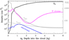Fig. 10

Structure of an isobaric PDR representing the most FUV-irradiated gas layers of the Orion Bar (see Table 2 for the adopted parameters). This plot shows the H₂, H, and electron density profiles (left axis scale), and the gas and dust temperatures (right axis scale).

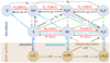Fig. 11

Main gas and grain reactions leading to the formation of sulfur hydrides. Red arrows represent endoergic reactions (endothermicity given in units of K). Dashed arrows are uncertain radiative associations (see Appendix A.3), γ stands for a FUV photon, and “s-” for solid.

Table 3

Column density predictions from different PDR models (up to A_V = 10 mag) and estimated values from observations (single-slab approach).

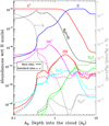Fig. 12

Pure gas-phase PDR models of the Orion Bar. Continuous curves show fractional abundances as a function of cloud depth, in logarithm scale to better display the irradiated edge of the PDR, using the new reaction rates listed in Table 1. The gray dotted curve shows f₂, the fraction of H₂ that is in vibrationally excited levels v ≥ 2 (right axis scale). Dashed curves are for a model using standard reaction rates.

6.2 Grain surface formation of solid H₂S

Similarly to the formation of water ice (s-H₂O) on grains (e.g., Hollenbach et al. 2009, 2012), the formation of H₂ S may be dominated by grain surface reactions followed by desorption back to the gas (e.g., Charnley 1997). Indeed, water vapor is relatively abundant in the Bar (N(H₂O) ≈ 10¹⁵ cm⁻²; Choi et al. 2014; Putaud et al. 2019) and large-scale maps show that the H₂ O abundance peaks close to cloud surfaces (Melnick et al. 2020).

To investigate the s-H₂S formation on grains, we updated the chemical model by allowing S atoms to deplete onto grains as the gas temperature drops inside the molecular cloud (for the basic grain chemistry formalism, see, Hollenbach et al. 2009). The timescale of this process (τ_{gr, S}) goes as $x {(S)}^{- 1}$ $x(\textrm{S})^{-1}$ $n_{H}^{- 1} T_{k}^{- 1 / 2}$ $n_{\textrm{H}}^{-1}\,T_{\textrm{k}}^{-1/2}$ , where x(S) is the abundance of neutral sulfur atoms with respect to H nuclei. In a PDR, the abundance of H atoms is typically higher than that of S atoms⁸ and H atoms stick on grains more frequently than S atoms unless x(H) <x(S)⋅0.18. An adsorbed H atom (s-H) is weakly bound, mobile, and can diffuse throughout the grain surface until it finds an adsorbed S atom (s-S). If the timescale for a grain to be hit by a H atom (τ_{gr, H}) is shorter that the timescale for a s-S atom to photodesorb (τ_{photdes, S}) or sublimate(τ_{subl, S}) then reaction of s-H with s-S will proceed and form a s-SH radical roughly upon “collision” and without energy barriers (e.g., Tielens & Hagen 1982; Tielens 2010). Likewise, if τ_{gr, H} <τ_{photdes, SH} and τ_{gr, H} <τ_{subl, SH}, a newly adsorbed s-H atom can diffuse, find a grain site with an s-SH radical and react without barriers to form s-H₂S. In these surface processes, a significant amount of S is ultimately transferred to s-H₂S (e.g., Vidal et al. 2017), which can subsequently desorb: thermally, by FUV photons, or by cosmic rays. In addition, laboratory experiments show that the excess energy of certain exothermic surface reactions can promote the direct desorption of the product (Minissale et al. 2016). In particular, reaction s-H + s-SH directly desorbs H₂ S with a maximum efficiency of ~60% (as observed in experiments, Oba et al. 2018). Due to the high flux of FUV photons in PDRs, chemical desorption may not always compete with photodesorption. However, it can be a dominant process inside molecular clouds (Garrod et al. 2007; Esplugues et al. 2016; Vidal et al. 2017; Navarro-Almaida et al. 2020).

The photodesorption timescale of an ice mantle is proportional to Y ⁻¹ $G_{0}^{- 1}$ $G_0^{-1}$ exp (+bA_V), where Y is the photodesorption yield (the number of desorbed atoms or molecules per incident photon) and b is a dust-related FUV field absorption factor. The timescale for mantle sublimation (thermal desorption) goes as $ν_{ice}^{- 1}$ $\nu_{\textrm{ice}}^{-1}$ exp (+E_b / k T_d), where ν_ice is the characteristic vibrational frequency of the solid lattice, T_d is the dust grain temperature, and E_b∕k is the adsorption binding energy of the species (in K). Binding energies play a crucial role in model predictions because they determine the freezing temperatures and sublimation timescales. Table 4 lists the E_b ∕k and Y values considered here.

Representative timescales of the basic grain processes described above are summarized in the upper panel of Fig. 13. In this plot, T_d is a characteristic dust temperature inside the PDR, T_d = (3 × 10⁴ + 2 × 10³ $G_{0}^{1.2}$ $G_{0}^{1.2}$ )^0.2, taken from Hollenbach et al. (2009). In the upper panel, the continuous black curve is the timescale for a grain to be hit by an H atom (τ_{gr, H}). The dashed magenta curves show the timescale for thermal desorption of an s-S atom (τ_{subl, S}) (left curve for E_b ∕k (S) = 1100 K and right curve for E_b∕k (S) = 2600 K), and the same for an s-O atom (blue curve). The gray dotted curve is the timescale for s-S atom photodesorption (τ_{photodes, S}) at A_V = 5 mag. At G₀ strengths where the continuous line is below the dashed and dotted lines, an adsorbed s-S atom remains on the grain surface sufficiently long to react with a diffusing s-H atom, form s-SH, and ultimately s-H₂S.

Figure 13 shows that, if one takes E_b ∕k (S) = 1100 K (the most common value in the literature; Hasegawa & Herbst 1993), the formation of s-H₂S is possible inside clouds illuminated by modest FUV fields, when grains are sufficiently cold (T_d < 22 K). However, recent calculations of s-S atoms adsorbed on water ice surfaces suggest higher binding energies (~ 2600 K; Wakelam et al. 2017). This would imply that S atoms freeze at higher T_d (≲ 50 K) and that s-H₂S mantles form in more strongly illuminated PDRs (the observed T_d at the edge of the Bar is ≃50 K and decreases to ≃35 K behind the PDR; see, Arab et al. 2012).

The freeze-out depth for sulfur in a PDR, the A_V at which most sulfur is incorporated as S-bearing solids (s-H₂S in our simple model) can be estimated by equating τ_{gr, S} and $τ_{photdes, H_{2} S}$ $\tau_{\textrm{photdes,\,H}_2\textrm{S}}$ . This implicitly assumes the H₂S chemical desorption does not dominate in FUV-irradiated regions, which is in line with the particularly large FUV absorption cross section of s-H₂S measured in laboratory experiments (Cruz-Diaz et al. 2014). With these assumptions, the lower panel of Fig. 13 shows the predicted s-H₂S and s-H₂O freeze-out depths. Owing to the lower abundance and higher atomic mass of sulfur atoms (i.e., grains are hit slower by S atoms than by O atoms), the H₂ S freeze-out depth appears slightly deeper than that of water ice. For the FUV-illumination conditions in the Bar, the freeze-out depth of sulfur is expected at A_V ≳ 6 mag. This implies that photodesorption of s-H₂S can produce enhanced abundances of gaseous H₂S at A_V < 6 mag.

FUV-irradiation and thermal desorption of H₂S ice mantles have been studied in the laboratory (e.g., Cruz-Diaz et al. 2014; Jiménez-Escobar & Muñoz Caro 2011). These experiments show that pure s-H₂S ices thermally desorb around 82 K, and at higher temperatures for H₂ S–H₂O ice mixtures. These experiments determine a photodesorption yield of $Y_{H_{2} S}$ $Y_{\textrm{H}_2\textrm{S}}$ ~ 1.2 × 10⁻³ molecules per FUV photon (see also Fuente et al. 2017). Regarding surface grain chemistry, experiments show that reaction s-H + s-SH → s-H₂S is exothermic (Oba et al. 2018), whereas reaction s-H + s-H₂S, although it has an activation energy barrier of ~1500 K, it may directly desorb gaseous SH. Finally, reaction s-SH + s-SH → s-H₂S₂ may trigger the formation of doubly sulfuretted species, but it requires mobile s-SH radicals (e.g., Jiménez-Escobar & Muñoz Caro 2011; Fuente et al. 2017). Here we will only consider surface reactions with mobile s-H.

Table 4

Adopted binding energies and photodesorption yields.

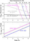Fig. 13

Representative timescales relevant to the formation of s-H₂S and s-H₂O as well as their freeze-out depths. Upper panel: the continuous black curve is the timescale for a grain to be hit by an H atom. Once in the grain surface, the H atom diffuses and can react with an adsorbed S atom to form s-SH. The dashed magenta curves show the timescale for thermal desorption of an s-S atom (E_b ∕k (S) = 1100 K left curve, and 2600 K right curve) and of an s-O atom (blue curve; E_b∕k (O) = 1800 K). The gray dotted curve is the photodesorption timescale of s-S. At G₀ values where the continuous line is below the dashed and dotted lines, s-O and s-S atoms remain on grain surfaces sufficiently long to combine with an adsorbed H atom and form s-OH and s-SH (and then s-H₂ O and s-H₂S). These timescales are for n_H = 10⁵ cm⁻³ and n(H) = 100 cm⁻³. Bottom panel: freeze-out depth at which most O and S are incorporated as s-H₂ O and s-H₂S (assuming no chemical desorption and T_k = T_d).

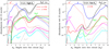Fig. 14

Gas-grain PDR models leading to the formation of s-H₂S (shown as black curves). Continuous colored curves show gas-phase fractional abundances as a function of depth into the cloud. ϵ refers to the efficiency of the chemical desorption reaction s-H + s-H₂S → SH + H₂ (see text). Left panel: gas-grain high E_b model (high adsorption binding energies for S and SH, see Table 4). Right panel: low E_b model.

6.3 Gas-grain PDR model results

Here we show PDR model results in which we add a simple network of gas-grain reactions for a small number of S-bearing (S, SH, and H₂ S) and O-bearing (O, OH, H₂O, O₂, and CO) species. These species can adsorb on grains as temperatures drop, photodesorb by FUV photons (stellar and secondary), desorb by direct impact of cosmic-rays, or sublimate at a given PDR depth (depending on T_d and on their E_b). Grain size distributions (n_gr ∝a^−3.5, where a is the grain radius) and gas-grain reactions are treated within the Meudon code formalism (see, Le Petit et al. 2006; Goicoechea & Le Bourlot 2007; Le Bourlot et al. 2012; Bron et al. 2014). As grain surface chemistry reactions we include s-H + s-X → s-XH and s-H + s-XH → s-H₂X, where s-X refers to s-S and s-O. In addition, we add the direct chemical desorption reaction s-H + s-SH → H₂S with an efficiency of 50% per reactive event, and also tested different efficiencies (ϵ) for the chemical desorption process s-H + s-H₂S → SH + H₂.

In our models we compute the relevant gas-grain timescales and atomic abundances at every depth A_V of the PDR. If the timescale for a grain to be struck by an H atom (τ_{gr, H}) is shorter than the timescales to sublimate or to photodesorb an s-X atom or a s-XH molecule; and if H atoms stick on grains more frequently than X atoms, we simply assume these surface reactions proceed instantaneously. At large A_V, larger than the freeze-out depth, this grain chemistry builds abundant s-H₂O and s-H₂S ice mantles.

Figure 14 shows results of two types of gas-grain models. The only difference between them is the adopted adsorption binding energies for s-S and s-SH. Left panel is for a “high E_b ” model and right panel is for a “low E_b” model (see Table 4). We note that these models do not include the gas-phase radiative association reactions S⁺ + H₂ → H₂S⁺ + hν and SH⁺ + H₂ → H₃S⁺ + hν; although their effect is smaller than in pure gas-phase models.

The chemistry of the most exposed PDR surface layers (A_V ≲ 2 mag) is the same to that of the gas-phase models discussed in Sect. 6.1. Photodesorption keeps dust grains free of ice mantles, and fast gas-phase ion-neutral reactions, photoreactions, and reactions with FUV-pumped H₂ drive the chemistry. The resulting SH⁺ abundance profile is nearly identical and there is no need to invoke depletion of elemental sulfur from the gas-phase to explain the observed SH⁺ emission (see Fig. 15). Beyond these first PDR irradiated layers, the chemistry does change because the formation of s-H₂S on grains and subsequent desorption alters the chemistry of the other S-bearing hydrides.

In model high E_b, S atoms start to freeze out closer to the PDR edge (T_d < 50 K). Because of the increasing densities and decreasing temperatures, the s-H₂S abundance with respect to H nuclei reaches ~10⁻⁶ at A_V ≃ 4 mag. In model low E_b, this level of s-H₂S abundance is only reachedbeyond an A_V of 7 mag. At lower A_V, the formation of s-H₂S on bare grains and subsequent photodesorption produces more H₂ S than pure-gas phase models independently of whether H₂S chemical desorption is included or not. In these intermediate PDR layers, at A_V ≃ 2–7 mag for the strong irradiation conditions in the Bar, the flux of FUV photons drives much of the chemistry, desorbing grain mantles, preventing complete freeze out, and dissociating the gas-phase products.

There are two H₂S abundance peaks at A_V ≃ 4 and 7 mag. The H₂S abundance in these “photodesorption peaks” depends on the amount of s-H₂S mantles formed on grains and on the balance between s-H₂S photodesorption and H₂S photodissociation (which now becomes the major source of SH). The enhanced H₂ S abundance modifies the chemistry of H₂ S⁺ and H₃ S⁺ as well: H₂S photoionization (with a threshold at ~10.4 eV) becomes the dominant source of H₂ S⁺ at A_V ≃ 4 mag because the H₂ (v ≥2) abundance is too low to make reaction (2) competitive. Besides, reactions of H₂ S with abundant molecular ions such as HCO⁺, H $_{3}^{+}$ $_{3}^{+}$ , and H₃ O⁺ dominate the H₃ S⁺ production.

Our gas-grain models predict that other S-bearing molecules, such as SO₂ and SO, can be the major sulfur reservoirs at these intermediate PDR depths. However, their abundances strongly depend on those of O₂ and OH through reactions S + O₂ → SO + O and SO + OH → SO₂ + H (see e.g., Sternberg & Dalgarno 1995; Fuente et al. 2016, 2019). These reactions link the chemistry of S- and O-bearing neutral molecules (Prasad & Huntress 1982) and are an important sink of S atoms at A_V ≳ 5 mag. However, while large column densities of OH have been detected in the Orion Bar (≳ 10¹⁵ cm⁻²; Goicoechea et al. 2011), O₂ remains undetected despite deep searches (Melnick et al. 2012). Furthermore, the inferred upper limit N(O₂) columns arebelow the expectations of PDR models (Hollenbach et al. 2009). This discrepancy likely implies that these gas-grain models miss details of the grain surface chemistry leading to O₂ (for other environments and modeling approaches see, e.g., Ioppolo et al. 2008; Taquet et al. 2016). Here we will not discuss SO₂, SO, or O₂ further.

At large cloud depths, A_V ≳ 8 mag, the FUV flux is largely attenuated, temperatures drop, the chemistry becomes slower, and other chemical processes dominate. The H₂ S abundance is controlled by the chemical desorption reaction s-H + s-SH → H₂S. This process keeps a floor of detectable H₂S abundances (>10⁻⁹) in regions shielded from stellar FUV radiation. In addition, and although not energetically favorable, the chemical desorption s-H + s-H₂S → SH + H₂ enhances the SH production at large A_V (the enhancement depends on the desorption efficiency ϵ), which in turn boosts the abundances of other S-bearing species, including that of neutral S atoms.

The H₂S abundances predicted bythe high E_b model reproduce the H₂S line intensities observed in the Bar (Sect. 6.4). In this model s-H₂S becomes the main sulfur reservoir. However, we stress that here we do not consider the formation of more complex S-bearing ices such as s-OCS, s-H₂S₂, s-S_n, s-SO₂ or s-HSO (Jiménez-Escobar & Muñoz Caro 2011; Vidal et al. 2017; Laas & Caselli 2019). Together with our steady-state solution of the chemistry, this implies that our predictions are not precise deep inside the PDR. However, we recall that our observations refer to the edge of the Bar, so it is not plausible that the model conditions at A_V ≳ 8 mag represent the line of sight we observe.

Model low E_b produces less H₂S in the PDR layers below A_V ≲ 8 mag because S atoms do not freeze until the dust temperature drops deep inside the PDR. Even beyond these layers, thermal desorption of s-S maintains higher abundances of S atoms at large depths. Indeed, model low E_b predicts that the major sulfur reservoir deep inside the cloud are gas-phase S atoms. This agrees with recent chemical models of cold dark clouds (Vidal et al. 2017; Navarro-Almaida et al. 2020).

6.4 Line intensity comparison and H₂S ortho-to-para ratio

We now specifically compare the SH⁺, SH, and H₂S line intensities implied by the different PDR models with the intensities observed toward the DF position of the Bar. We used the output of the PDR models – T_k, T_d, n(H₂), n(H), n_e, n(SH⁺), n(SH), and n(H₂S) profiles fromA_V = 0 to 10 mag – as input for a multi-slab Monte Carlo model of their line excitation, including formation pumping (formalism presented in Sect. 4) and radiative transfer. As the Orion Bar is not a perfectly edge-on, this comparison requires a knowledge of the tilt angle (α) with respect to a pure edge-on PDR. Different studies suggest α of ≈5° (e.g., Jansen et al. 1995; Melnick et al. 2012; Andree-Labsch et al. 2017). This inclination implies an increase in line-of-sight column density, compared to a face-on PDR, by a geometrical factor (sin α)⁻¹. It also means that optically thin lines are limb-brightened.

The left panel of Fig. 15 shows SH⁺ line intensity predictions for isobaric PDR models of different P_th values (leading to different T_k and n_H profiles). Since the bulk of the SH⁺ emission arises from the PDR edge (A_V ≃ 0 to 2 mag) all models (gas-phase or gas-grain) give similar results. The best fit is for P_th ≃ (1–2) × 10⁸ cm⁻³ K and α ≃ 5°. These high pressures, at least close to the DF, agree with those inferred from ALMA images of HCO⁺ (J = 4–3) emission (Goicoechea et al. 2016), Herschel observations of high-J CO lines (Joblinet al. 2018), and IRAM 30 m detections of carbon recombination lines (Cuadrado et al. 2019).

Right panel of Fig. 15 shows SH and H₂ S line emission predictions for the high E_b gas-grain model (magenta squares), low E_b gas-grain model (gray triangles), and a pure gas-phase model (cyan circles). For each model, the upper limit intensities refer to radiative transfer calculations with an inclination angle α = 5°. The lower intensity limits refer to a face-on PDR. Gas-phase models largely underestimate the observed H₂ S intensities. Model low E_b produces higher H₂S columns and brighter H₂S lines, but still below the observed levels (by up to a factor of ten). Model high E_b provides a good agreement with observations; the two possible inclinations bracket the observed intensities, and it should be considered as the reference model of the Bar. It is also consistent with the observational SH upper limits.

Our observations and models provide a (line-of-sight) N(o-H₂S)/N(p-H₂S) OTP ratio of 2.9 ± 0.3, consistent with the (gas-phase) high-temperature statistical equilibrium value. However, the cold “nuclear-spin-temperatures” (T_spin ≪T_k; see definition in Eq. (D.1)) implied by the low water vapor OTP ratios observed in some sources (< 2.5) have been associated with the temperature of the ice mantles where H₂ O molecules might have formed (i.e., T_spin ≃ T_d; Mumma et al. 1987; Lis et al. 2013). In the case of H₂S, our derived OTP ratio toward the DF position implies any T_spin above 30 ±10 K (see Fig. D.1). Hence, this temperature might be also compatible with s-H₂S formation⁹ in warm grains if T_spin ≃ T_d upon formation is preserved in the gas-phase after photodesorption (e.g., Guzmán et al. 2013). Interestingly, the H₂ O OTP ratio derived from observations of the Orion Bar is 2.8 ± 0.1 (Putaud et al. 2019) and implies T_spin(H₂O) = 35 ± 2 K. This value is compatible with T_spin(H₂S) and might reflect the similar T_d of the PDR layers where most s-H₂O and s-H₂S form and photodesorb. Nevertheless, laboratory experiments have challenged this T_spin ≃T_d association, at least for s-H₂O: cold water ice surfaces, at 10 K, photodesorb H₂O molecules with an OTP ratio of ~3 (Hama et al. 2016). Follow up observations of p-H₂S lines across the Bar will allow us to study possible variations of the OTP ratio as G₀ diminishes and grains get colder.

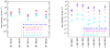Fig. 15

Line intensity predictions for different isobaric PDR models. Calculations were carried out in a multi-slab Monte Carlo code (Sect. 4) that uses the output of the PDR model. Blue stars show the line intensities observed toward the Bar (corrected by beam dilution). Left panel: SH⁺ emission models for PDRs of different P_th values and α = 5°. Right panel: SH and H₂S (adopting anOTP ratio of 3) emission from: high E_b (magenta squares), low E_b (gray triangles), and gas-phase (cyan circles) PDR models, all with P_th / k = 2 × 10⁸ K cm⁻³. Upper limit intensity predictions are for a PDR with an inclination angle of α = 5° with respectto a edge-on geometry. Lower limit intensities refer to a face-on PDR model.

6.5 Generalization to different G₀ and n_H conditions

In this section we generalize our results to a broader range of gas densities and FUV illumination conditions (i.e., to clouds with different G₀ / n_H ratios). We run several PDR models using the high E_b gas-grain chemistry. The main difference compared to the Orion Bar models is that here we model constant density clouds with standard interstellar grain properties (R_V = 3.1). Figure 16 (left panel) shows models of clouds with constant n_H = 10⁴ cm⁻³ and varying FUV radiation fields, while Fig. 16 (right panel) show models of constant FUV illumination (G₀ = 100) and varying gas densities¹⁰. The main result of this study is the similar gas-phase H₂S column density (a few 10¹⁴ cm⁻² up to A_V = 10) and H₂ S abundance peak (a few 10⁻⁸ close to the FUV-irradiated cloud edge) predicted by these models nearly irrespective of G₀ and n_H. A similar conclusion was reached previously for water vapor in FUV-illuminated clouds (Hollenbach et al. 2009, 2012). Increasing G₀ shifts the position of the H₂ S abundance peak to larger A_V until the rate of S atoms sticking on grains balances the H₂S photodissociation rate (the dominant H₂S destruction mechanism except in shielded gas; see also Fig. 13). Since s-H₂S photodesorption and H₂S photodissociation rates depend on G₀, the peak H₂S abundance in the PDR is roughly the same independently of G₀. On the other hand, the formation rate of s-H₂S mantles depends on the product n(S) n_gr ∝ $n_{H}^{2}$ $n_{\textrm{H}}^{2}$ , whereas the H₂S photodesorption rate depends on n_gr ∝n_H. Hence, the H₂S abundance peak moves toward the cloud surface for denser PDRs (like the Orion Bar). The exact abundance value depends on the adopted grain-size distribution and on the H₂S photodesorption yield (which is well constrained by experiments; see, Cruz-Diaz et al. 2014; Fuente et al. 2017).

The roleof chemical desorption increases and can dominate beyond the photodesorption peak as the flux of stellar FUV photons is attenuated. Here we do not carry out an exhaustive study of this mechanism, which is hard to model in full detail because its efficiency decreases considerably with the properties of grain surfaces (bare vs. icy; see e.g., Minissale & Dulieu 2014). In our models, and depending on ζ_CR, photodesorption by secondary FUV photons can also be important in cloud interiors. These processes limit the conversion of most of the sulfur reservoir into S-bearing ices and increase the abundance of other gas-phase species deep inside clouds, notably S atoms and H₂ S molecules.

The H₂S abundance in shielded gas depends on the destruction rate by gas-phase reactions different than photodissociation, in particular H₂ S reactions with H $_{3}^{+}$ $_{3}^+$ . The H $_{3}^{+}$ $_{3}^+$ abundance increases with ζ_CR and decreases with the electron density. Figure 16 (right) shows models of constant G₀ and constant ζ_CR in which the H₂S abundance at large depths increases with decreasing density (more penetration of FUV photons, more ionization, more electrons, less H $_{3}^{+}$ $_{3}^+$ ). The lowest gas density model, n_H = 10³ cm⁻³, shows the highest H₂S abundance at large A_V. Because S freeze-out is less efficient at low densities, the low-density model shows higher gas-phase S abundances at large depths, making atomic S a dominant gas-phase sulfur reservoir. Unfortunately, direct observation of atomic S in cold gas is complicated, which makes it difficult to benchmark this prediction.

In warm PDRs, in addition to S radio recombination lines (e.g., Smirnov et al. 1995), the ³ P fine-structure lines of atomic sulfur, the [S I] 25, 56 μm lines, can be interesting diagnostics of gas physical conditions and of [S/H] abundances. Unfortunately, the low sensitivity of previous infrared telescopes was not sufficient to detect the [S I] 25 μm line (ΔE₁₂ = 570 K) in the Orion Bar (Rosenthal et al. 2000); although it is detected in protostellar outflows (e.g., Neufeld et al. 2009; Goicoechea et al. 2012). Moreover, the ³ P₂-¹D₂ forbidden line of atomic sulfur at 1.082 μm can be an interesting tracer of the ionization and dissociation fronts in PDRs. Some of these lines will be accesible to high-angular-resolution and high sensitivity observations with JWST.

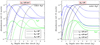Fig. 16

Constant density gas-grain PDR models using the high E_b chemical network and undepleted sulfur elemental abundances. Left panel: effects of changing the FUV radiation field. Right panel:effects of varying the gas density.

6.6 The origin of H₂S emission in other environments

Irrespective of n_H and G₀, grain surface formation of s-H₂S and photodesorption back to the gas-phase lead to H₂ S column densities of a few 10¹⁴ cm⁻² in PDRs. This is in agrement with the observed column in the Bar (G₀ ≈ 10⁴) as well as at the mildly illuminated rims of TMC-1 and Barnard 1b clouds (G₀ ≈ 10; Navarro-Almaida et al. 2020). The inferred H₂ S abundance in the interior of these dark clouds (A_V > 10 mag) drops to a few 10⁻⁹, but the species clearly does not disappear from the gas (N(H₂S) of a few 10¹³ cm⁻²; Navarro-Almaida et al. 2020). Interestingly, neither in the Bar the H₂S line emission at ~168 GHz decreases much behind the PDR (Fig. 1) even if the flux of FUV photons is largely attenuated compared to the irradiated PDR edge.

Despite oxygen is ~25 times more abundant than sulfur, the H₂O to H₂S column density ratio in the Orion Bar PDR is only about ~5. This similarity must also reflect the higher abundances of CO compared to CS. Furthermore, the H₂ S column density in cold cores is strikingly similar to that of water vapor (Caselli et al. 2010, 2012). This coincidence points to a more efficient desorption mechanism of s-H₂S compared tos-H₂O in gas shielded from stellar FUV photons. Navarro-Almaida et al. (2020) argues that chemical desorption is able to reproduce the observed H₂S abundance floor if the efficiency of this process diminishes as ice grain mantles get thicker inside cold dense cores.

Turning back to warmer star-forming environments, our predicted H₂ S abundance in FUV-illuminated gas is comparable to that observed toward many hot cores (~10⁻⁹–10⁻⁸; van der Tak et al. 2003; Herpin et al. 2009). In these massive protostellar environments, thermal desorption of icy mantles, suddenly heated to T_d ≳ 100 K by the luminosity of the embedded massive protostar, drives the H₂ S production. Early in their evolution, young hot cores (≲10⁴ yr) can show even higher abundances of recently desorbed H₂ S (before further chemical processing takes place in the gas-phase; e.g., Charnley 1997; Hatchell et al. 1998; Jiménez-Serra et al. 2012; Esplugues et al. 2014). Indeed, Crockett et al. (2014) reports a gas-phase H₂ S abundance of several 10⁻⁶ toward the hot core in Orion KL. This high value likely reflects the minimum s-H₂S abundance locked as s-H₂S mantles just before thermal desorption. In addition, the H₂S abundance in the Orion Bar is only slightly lower than that inferred in protostellar outflows (several 10⁻⁸). In these regions, fast shocks erode and sputter the grain mantles, releasing a large fraction of their molecular content and activating a high-temperature gas-phase chemistry that quickly reprocesses the gas (e.g., Holdship et al. 2019). All in all, it seems reasonable to conclude that everywhere s-H₂S grain mantles form, or already formed in a previous evolutionary stage, emission lines from gas-phase H₂ S will be detectable.

In terms of its detectability with single-dish telescopes, H₂ S rotational lines are bright in hot cores (T_{peak, 168 GHz} ≃ 30 K in Orion KL but ≃ 1–3 K toward most hot cores; Tercero et al. 2010; van der Tak et al. 2003; Herpin et al. 2009), in strongly irradiated PDRs (≃6 K, this work), and in lower-illumination PDRs such as the Horsehead (≃1 K; Rivière-Marichalar et al. 2019). The H₂S emission is fainter toward cold dark clouds (≃ 0.2 K in TMC-1; Navarro-Almaida et al. 2020) and protostellar outflows (≃ 0.6 K in L1157; Holdship et al. 2019). These line intensity differences are mostly produced by different gas physical conditions and not by enormous changes of the H₂S abundance.

Finally, H₂S is also detected outside the Milky Way (firstly by Heikkilä et al. 1999). Lacking enough spatial-resolution it is more difficult to determine the origin of the extragalactic H₂S emission. The derived abundances in starburst galaxies such as NGC 253 (~10⁻⁹; Martín et al. 2006)might be interpreted as arising from a collection of spatially unresolved hot cores (Martín et al. 2011). However, hot cores have low filling factors at star-forming cloud scales. Our study suggests that much of this emission can arise from (the most common) extended molecular gas illuminated by stellar FUV radiation (e.g., Goicoechea et al. 2019).

7 Summary and conclusions

We carried out a self-consistent observational and modeling study of the chemistry of S-bearing hydrides in FUV-illuminated gas. We obtained the following results:

ALMAimages of the Orion Bar show that SH⁺ is confined to narrow gas layers of the PDR edge, close to the H₂ dissociation front. Pointed observations carried out with the IRAM 30 m telescope show bright H $_{2}^{32}$ $_{2}^{32}$ S, H $_{2}^{34}$ $_{2}^{34}$ S, H $_{2}^{33}$ $_{2}^{33}$ S emission toward the PDR (but no H₃ S⁺, a key gas precursor of H₂S) as well as behind the Bar, where the flux of FUV photons is largely attenuated. SOFIA observations provide tight limits to the SH emission.
The SH⁺ line emission arises from a high-pressure gas component, P_th ≃ (1–2) × 10⁸ cm⁻³ K, where SH⁺ ions are destroyed by reactive collisions with H atoms and electrons (as most H_n S⁺ ions do). We derive N(SH⁺) ≃ 10¹³ cm⁻² and an abundance peak of several ~10⁻⁹. H₂ S shows larger column densities toward the PDR, N(H₂S) = N(o-H₂S) + N(p-H₂S) ≃ 2.5 × 10¹⁴ cm⁻². Our tentative detection of SH translates into an upper limit column density ratio N(SH)/N(H₂S) of < 0.2–0.6, already lower than the ratio of 1.1–3.0 observed in low-density diffuse molecular clouds (Neufeld et al. 2015). This implies an enhanced H₂ S production mechanism in FUV-illuminated dense gas.
All gas-phase reactions X + H₂ (v = 0) → XH + H (with X = S⁺, S, SH⁺, or H₂ S⁺) are highly endoergic. While reaction of FUV-pumped H₂ (v ≥ 2) molecules with S⁺ ions becomes exoergic and explains the observed levels of SH⁺, further reactions of H₂ (v ≥ 2) with SH⁺ or with neutral S atoms, both reactions studied here through ab initio quantum calculations, do not form enough H₂ S⁺ or H₃ S⁺ to ultimately produce abundant H₂S. In particular, pure gas-phase models underestimate the H₂S column density observed in the Orion Bar by more than two orders of magnitude. This implies that these models miss the main H₂ S formation route. The disagreement is even worse as we favor, after considering the potential energy surfaces of the H₂ S^+* and H₃ S^+* complexes, that the radiative associations S⁺ + H₂ → H₂S⁺ + hν and SH⁺ + H₂ → H₃S⁺ + hν may actually not occur or possess slower rates than considered in the literature.
To overcome these bottlenecks, we built PDR models that include a simple network of gas-grain and grain surface reactions. The higher binding energies of S and SH suggested by recent studies imply that bare grains start to grow s-H₂S mantles notfar from the illuminated edges of molecular clouds. Indeed, the observed N(H₂S) in the Orion Bar can only be explained by the freeze-out of S atoms, grain surface formation of s-H₂S mantles, and subsequent photodesorption back to the gas phase. The inferred H₂ S OTP ratio of 2.9 ± 0.3 (equivalent to T_spin ≥ 30 K) is compatible with the high-temperature statistical ratio as well as with warm grain surface formation if T_spin ≃T_d and if T_spin is preserved inthe gas-phase after desorption.
Comparing observations with chemical and excitation models, we conclude that the SH⁺-emitting layers at the edge of the Orion Bar (A_V < 2 mag) are charaterized by no or very little depletion of sulfur from the gas-phase. At intermediate PDR depths (A_V < 8 mag) the observedH₂S column densities do not require depletion of elemental (cosmic) sulfur abundances either.
We conclude that everywhere s-H₂S grain mantles form (or formed) gas-phase H₂S will be present in detectable amounts. Independently of n_H and G₀, FUV-illuminated clouds produce roughly the same H₂S column density (a few 10¹⁴ cm⁻²) and H₂S peak abundances (a few 10⁻⁸). This agrees with the H₂S column densities derived in the Orion Bar and at the edges of mildly illuminated clouds. Deep inside molecular clouds (A_V > 8 mag), H₂ S still forms by direct chemical desorption and photodesorption by secondary FUV photons. These processes alter the abundances of other S-bearing species and makes difficult to predict the dominant sulfur reservoir in cloud interiors.

In this study we focused on S-bearing hydrides. Still, many subtle details remain to be fully understood: radiative associations, electron recombinations, and formation of multiply sulfuretted molecules. For example, the low-temperature (T_k < 1000 K) rates of the radiative and dielectronic recombination of S⁺ used in PDR models may still be not accurate enough (Badnell 1991). In addition, the main ice-mantle sulfur reservoirs are not fully constrained observationally. Thus, some of the narrative may be subject to speculation. Similarly, reactions of S⁺ with abundant organic molecules desorbed from grains (such as s-H₂CO, not considered in our study) may contribute to enhance the H₂ S⁺ abundance through gas-phase reactions (e.g., S⁺ +H₂CO → H₂S⁺+CO; Prasad & Huntress 1982). Future observations of the abundance and freeze out depths of the key ice carriers with JWST will clearly help in these fronts.

Acknowledgements

We warmly thank Prof. György Lendvay for interesting discussions and for sharing the codes related to their S(³ P) + H₂ ( $^{1} Σ_{g}^{+}$ $^1\Sigma_g^+$ ,v) PES. We thank Paul Dagdigian, François Lique, and Alexandre Faure for sharing their H₂ S–H₂, SH⁺–H, and SH⁺–e⁻ inelastic collisional rate coefficients and for interesting discussions in Grenoble and Salamanca. We thank Helgi Hrodmarsson for sending his experimental SH photoionization cross section in tabulated format. We finally thank our referee, John H. Black, for encouraging and insightful suggestions. This paper makes use of the ALMA data ADS/JAO.ALMA#2012.1.00352.S. ALMA is a partnership of ESO (representing its member states), NSF (USA), and NINS (Japan), together with NRC (Canada), and NSC and ASIAA (Taiwan), in cooperation with the Republic of Chile. The Joint ALMA Observatory is operated by ESO, AUI/NRAO, and NAOJ. It also includes IRAM 30 m telescope observations. IRAM is supported by INSU/CNRS (France), MPG (Germany), and IGN (Spain). We thank the staff at the IRAM 30 m telescope and the work of the USRA and NASA staff of the Armstrong Flight Research Center in Palmdale and of the Ames Research Center in Mountain View (California), and the Deutsches SOFIA Institut. Wethank the Spanish MICIU for funding support under grants AYA2016-75066-C2-2-P, AYA2017-85111-P, FIS2017-83473-C2 PID2019-106110GB-I00, and PID2019-106235GB-I00 and the French-Spanish collaborative project PICS (PIC2017FR). We finally acknowledge computing time at Finisterrae (CESGA) under RES grant ACCT-2019-3-0004.

Appendix A H₂S⁺ formation and destruction

In this appendix we give details about how we calculated the H₂ vibrational-state-dependent rates of reaction (2) and of the reverse reaction, the destruction of H₂ S⁺ (²A′) by reactive collisons with H (²S) atoms (summarized in Fig. A.1).

We first built a full dimensional potential energy surface (PES) of the triplet H₃ S⁺ (³A) system by fitting more than 150 000 ab initio points, including the long range interactions in the reactants and products channels. The main topological features of the PES are summarized in the minimum energy path between reactants and products (see middle panel of Fig. 9). These ab initio points were calculated with an explicitly correlated restricted coupled cluster including a single, double, and (perturbatively) triple excitations (RCCSD(T)-F12a) method (Knizia et al. 2009). The analytical fit has a overall rms error of ≃ 0.01 eV (Fig. A.2). Appendix A.1 provides more details.

Reaction (2) is endothermic by 0.672 eV, and the PES of the triplet state shows two shallow wells in the H₂ + SH⁺ entrance channel (named ³W_1a and ³ W_1b, with a depth of ≃0.118 eV) and another one near the H + H₂ S⁺ products (named ³W₂, with a depth of 0.08 eV). Between the reactants and products wells there is a saddle point, with an energy of 0.601 eV. This saddle point, slightly below the products, has a geometry similar to ³ W₂ in which the H–H distance is strongly elongated compared to that of H₂. These features are also present in the maximum multiplicity PES of reactions H₂ + S $^{+} (^{4} S)$ $^+(^4S)$ and H₂ + H₂ S⁺(²A) (see Fig. 9). We determine the state-dependent rates of reaction (2) and of the reverse reaction using a quasi-classical trajectory (QCT) method on our ground triplet PES. We provide more details on how the reactive cross sections for fixed collision energies were calculated in Appendix A.2.

The formation rate of H₂ S⁺ from H₂ (v = 0) is very slow. For H₂ (v = 1), the rate constant significantly increases at ≈500 K, corresponding with the opening of the H₂ S⁺ + H threshold. At this point, it is important to consider the zero-point energy (ZPE) of the products (see next section for details). For H₂ (v = 2) and H₂ (v = 3), reaction rates are faster, close to the Langevin limit. Finally, the H₂ S⁺ destruction rate constant is very similar to that of its formation from H₂ (v = 2). In Appendix A.3 we provide more information about the destruction of H_n S⁺ ions through radiative association and spin flip mechanisms.

A.1 Ab initio calculations and PES

Dagdigian (2019b) presented a PES for the SH⁺-H₂ system that includes 4-dimensions and is based on RCCSD(T)-F12a ab initio calculations. This PES was used to study SH⁺–H₂ inelastic collisions using a rigid rotor approach in which the two diatomic molecules are kept fixed at their equilibrium distances. However, in order to study the reactivity of the collision, the two diatomic distances have to be included to account for the breaking and formation of new bonds.

Reaction (2) corresponds to a triplet state H₃S⁺ (³A). The H₂S⁺ (²A′) + H (²S) products can form a triplet and a singlet state. The triplet state can lead to the destruction of H₂S⁺ through reaction with H atoms. The singlet state, however, produces very excited states of the reactants. Thus, it only leads to inelastic collisions but not not to the destruction of H₂S $^{+} (^{2} A^{'})$ $^+(^2A')$ . In consequence, here we only consider the ground triplet electronic state of the system. In addition, the H $_{3}^{+}$ $_3^+$ + S (³P) channel is about 2.4 eV above the H₂ + SH⁺ asymptote, and will not be included in the present study.

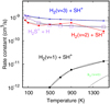Fig. A.1

Calculated rate constants as a function of temperature (for translation and rotation) for SH⁺ (v = 0, j = 0) + H₂ (v = 1, 2, 3, j = 0) and H₂S⁺ (v = 0, j = 0) + H reactions (lavender) using ZPE corrected QCT method. Dotted curves are fits of the form k(T) = α (T/300)^β exp(−γ∕T). Rate coefficients are listed in Table 1.

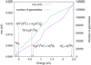Fig. A.2

Rms error as a function of total energy, showing the number of ab initio points used to evaluate the error in the PES calculation. Arrows indicate selected critical points in the PES and provide an estimate of the error in each region. TS means transition state.

In order to study the regions where several electronic states intersect, we performed a explicitly correlated internally contracted multireference configuration interaction (ic-MRCI-F12) calculation (Shiozaki & Werner 2013; Werner & Knowles 1988a,b) including the Davidson correction (icMRCI-F12+Q; Davidson 1975). The ic-MRCI-F12 calculations were carried out using state-averaged complete active space self-consistent field (SA-CASSCF) orbitals with all the CAS configurations as the reference configuration state functions. We used a triple zeta correlation consistent basis set for explicitly correlated wave functions (cc-pVTZ-F12; Peterson et al. 2008). In order to avoid orbital flipping between core and valence orbitals. SA-CASSCF calculations with three lowest triplet states were carried out including the core and valence orbitals as active space (18 electrons in 11 orbitals). For the ic-MRCI-F12 calculation, the core orbitals was kept doubly occupied, resulting in about 2.5 × 10⁶ (9 × 10⁷) contracted (uncontracted) configurations. All ab initio calculations were performed with MOLPRO (Werner et al. 2012).

Our ic-MRCI-F12 calculations show that the crossings with electronic excited states are 2 eV above the energy of the reactants. The energy interval below 2 eV is enough to study reaction (2). In these low-energy regions, RCCSD(T)-F12a calculations were also performed. They are in good agreement with the ic-MRCI-F12 results and the t₁ diagnostic is always below 0.03. This allows us to conclude that for energies below 2 eV, the RCCSD(T)-F12a method performs well, presents a simple convergence, and being size consistent, is well adapted to the present case. This method is the same one employed in the inelastic collision calculations by Dagdigian (2019b).

We performed extensive RCCSD(T)-F12a calculations in all accessible regions to properly describe the six-dimensional phase space. 150 000 ab initio points were fitted to a multidimensional analytic function, that generates the six-dimensional PES represented as $H = H^{diab} + H^{MB}$ $\begin{eqnarray*}H\,{=}\, H^{\textrm{diab}} + H^{\textrm{MB}} \end{eqnarray*}$ (A.1)

(Aguado et al. 2010; Sanz-Sanz et al. 2013; Zanchet et al. 2018; Roncero et al. 2018), where H^diab is an electronic diabatic matrix in which each diagonal matrix element describes a rearrangement channel – six in this case, three equivalent for SH⁺ + H₂ channels, and three equivalent for H₂ S⁺ + H fragments (we omitted the H $_{3}^{+}$ $_3^+$ + S channel) – as an extension of the reactive force field approach (Farah et al. 2012). In each diagonal term, the molecular fragments (SH⁺, H₂ and H₂ S⁺) are described by 2 or 3 body fits (Aguado & Paniagua 1992), and the interaction among them is described by a sum of atom-atom terms plus the long range interaction. The non diagonal terms of H^diab are described aspreviously (Zanchet et al. 2018; Roncero et al. 2018) and the parameters are fitted to approximately describe the saddle points along the minimum energy path in the right geometry.

In the reactants channel, the leading long range interaction $S H^{+} (X^{3} Σ^{-}) + H_{2} (X^{1} Σ_{g}^{+})$ ${SH}^+(X^3\Sigma^-) + {H}_2(X^1\Sigma_g^+)$ corresponds to charge-quadrupole and charge-induced dipole interactions (Buckinghan 1967): $\begin{array}{l} V_{c h a r g e} (r_{HH}, R) = Θ_{2} (r_{HH}) P_{2} (\cos θ_{2}) R^{- 3} \\ - [\frac{1}{2} α_{0} (r_{HH}) + \frac{1}{3} (α_{∥} (r_{HH}) - α_{⊥} (r_{HH})) P_{2} (\cos θ_{2})] R^{- 4} \end{array}$ $\begin{eqnarray*} && \hspace*{-6pt} V_{{charge}}(\mathbf{r}_{\textrm{HH}},\mathbf{R})\,{=}\,\Theta_2 (r_{\textrm{HH}}) P_2(\cos \theta_2) R^{-3} \nonumber\\ &&\hspace*{-6pt} \quad - \left[ \frac12 \alpha_0(r_{\textrm{HH}}) + \frac{1}{3} \left(\alpha_{\parallel}(r_{\textrm{HH}})-\alpha_{\perp}(r_{\textrm{HH}}) \right)P_2(\cos \theta_2) \right] R^{-4} \end{eqnarray*}$ (A.2)

and the dipole-quadrupole interactions (Buckinghan 1967): $\begin{array}{l} V_{d i p o l e} (r_{SH}, r_{HH}, R) = 3 μ_{1} (r_{SH}) Θ_{2} (r_{HH}) \\ \times [\cos θ_{1} P_{2} (\cos θ_{2}) + \sin θ_{1} \sin θ_{2} \cos θ_{2} \cos ϕ] R^{- 4}, \end{array}$ $\begin{eqnarray*} && \hspace*{-6pt}V_{{dipole}}(\mathbf{r}_{\textrm{SH}}, \mathbf{r}_{\textrm{HH}},\mathbf{R})\,{=}\,3 \mu_1 (r_{\textrm{SH}}) \Theta_2 (r_{\textrm{HH}}) \nonumber\\ && \hspace*{-6pt} \quad {\times}\, \left[ \cos \theta_1 P_2(\cos \theta_2) + \sin \theta_1 \sin \theta_2 \cos \theta_2 \cos \phi \right] R^{-4}, \end{eqnarray*}$ (A.3)

where Θ₂(r_HH) is the cuadrupole moment of $H_{2} (X^{1} Σ_{g}^{+})$ ${H}_2(X^1\Sigma_{\textrm{g}}^+)$ , α₀ (r_HH), α_∥ (r_HH), and α_⊥ (r_HH) are the average, parallel, and perpendicular polarizabilities of $H_{2} (X^{1} Σ_{g}^{+})$ ${H}_2(X^1\Sigma_{\textrm{g}}^+)$ , respectively,and μ₁(r_SH) is the dipole moment of SH⁺(X³Σ⁻). P₂ (cosθ) represents the Legendre polynomial of degree 2. The dependence of the molecular properties of H₂ with the interatomic distance r_HH is obtained from Velilla et al. (2008). The dipole moment of SH⁺ depends on the origin of coordinates. Since SH⁺(X³Σ⁻) dissociates in $S^{+} (^{4} S) + H (^{2} S)$ ${S}^+(^4S) + {H}(^2S)$ , we select the origin of coordinates in the S atom, so that the dipole moment tends to zero when R goes to infinity.

Table A.1

RCCSD(T)-F12a and fit stationary points on the PES.

Table A.2

E_v of reactants and products, and adiabatic switching energies for the QCT initial conditions.

In the products channel, the long range interaction $H_{2} S^{+} (X^{2} A^{″}) + H (^{2} S)$ ${H}_2{S}^+\,(X^2 A'')\,+\,{H}\,(^2S)$ corresponds to the isotropic charge-induced dipole and charge-induced quadrupole dispersion terms $V_{d i s p} (R) = - \frac{9}{4} R^{- 4} - \frac{15}{4} R^{- 6} .$ $\begin{equation*} V_{{disp}}(R)\,{=}\,-\frac{9}{4} R^{-4} -\frac{15}{4} R^{-6}. \end{equation*}$

These long range terms diverge at R = 0. To avoid this behavior, we replace R by $R$ ${\cal R}$ : $R = R + R_{0} e^{- (R - R_{e})} with R_{0} = 10 bohr .$ $\begin{equation*} {\cal R}\,{=}\,R + R_0 e^{-(R-R_e)} \quad\quad{\textrm{with}}\quad\quad R_0\,{=}\, 10\, \textrm{bohr.} \end{equation*}$

In Eq. (A.1), H^MB is the many-body term, which is described by permutationaly invariant polynomials following the method of Aguado an collaborators (Aguado & Paniagua 1992; Tablero et al. 2001; Aguado et al. 2001). This many-body term improves the accuracy of the PES, especially in the region of the reaction barriers (as shown in Fig. 9). Features of the stationary points are listed in Table A.1.

A.2 Determination of reactive collision rates

We studied the reaction dynamics using a quasi-classical trajectory (QCT) method with the code miQCT (Zanchet et al. 2018; Roncero et al. 2018). In this method, the initial vibrational energy of the reactants is included using the adiabatic switching method (AS) (Grozdanov & Solov’ev 1982; Johnson 1987; Qu & Bowman 2016; Nagy & Lendvay 2017). Energies arelisted in Table A.2. The initial distance between the center-of-mass of the reactants (H₂ + SH⁺ or H₂ S⁺ + H) is set to 85 bohr, and the initial impact parameter is set randomly within a disk, the radius of which is set according to a capture model (Levine & Bernstein 1987) using the corresponding long-range interaction. The orientation among the two reactants is set randomly.

A first exploration of the reaction dynamics is done at fixed collision energy, for H₂ (v = 0, 1, 2, 3) + SH⁺ (v = 0) and H + H₂ S⁺(v = 0), and the reactive cross section is calculated as in Karplus et al. (1965) $σ_{v j} (E) = π b_{max}^{2} P_{r} (E) with P_{r} (E) = \frac{N_{r}}{N_{tot}},$ $\begin{eqnarray*}\sigma_{vj}(E)\,{=}\, \pi b_{\textrm{max}}^2 P_{\textrm{r}}(E) \quad {\textrm{with }}\quad P_{\textrm{r}}(E)\,{=}\, {N_{\textrm{r}}\over N_{\textrm{tot}}}, \end{eqnarray*}$ (A.4)

where N_t is the maximum number of trajectories with initial impact parameter lower than b_max, the maximum impact parameter for which the reaction takes place, and N_r is the number of trajectories leading to products. Figure A.2 shows results for N_t > 20 000 and all energies and initial reactant and vibrational states.

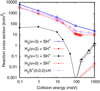Fig. A.3

Reaction cross section (in bohr²) as a function of collision energy (in meV) for the SH⁺ (v = 0, j = 0) + H₂ (v = 1, 2, 3, j = 0) and H₂S⁺ (v = 0, j = 0) + H collisions. Filled symbols are obtained counting all trajectories leading to products, while open symbols correspond to the ZPE corrected ones.

For the SH⁺ (v = 0, j = 0) + H₂ (v, j = 0) reaction there is a strong dependence on the initial vibrational state. For H₂ (v = 0), there is nearly no reactive event, and only at 1 eV there are some reactive trajectories. For H₂ (v = 2 and 3), however, the reaction shows a relatively large cross section, that decreases with increasing collision energy, as expected for exoergic reactions. Energies below 10–100 meV are dominated by long range interactions, leading to an increase in the maximum impact parameter, b_max, consistent with the variation of the cross section.

Reaction SH⁺ (v = 0, j = 0) + H₂ (v = 1, j = 0) shows an unexpected behavior that deserves some discussion. At energies below 40 meV, the cross section is large and decreases with increasing energy. In the 40–200 meV that is consistent with the endothermicity of the reaction.

In order to analyze the reaction mechanism for H₂ (v = 1) below 40 meV, we carried out an extensive analysis of the trajectories. A typical one is presented in Fig. A.4 for 10 meV. The H₂ and SH⁺ reactants are attracted to each other by long range interactions, until they get trapped in the ³ W₁ wells, as it is shown by the evolution of R, the distancebetween center-of-mass of the two molecules. The trapping lasts for 8 ps, thus allowing several collisions between H₂ and SH⁺ and permitting the energy transfer between them. The H₂ molecule ultimately breaks, and leaves SH⁺ with less vibrational energy. This can be inferred from the decrease in the amplitudes of the SH⁺ distance. The energy of the H₂ S⁺ product is below the ZPE (see Table A.2). This is a clear indication of ZPE leakage in the QCT method, due to the energy transfer promoted by the long-lived collision complex.

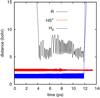Fig. A.4

H–H, SH⁺ and R distances(in bohr) versus time (in ps), for a typical reactive trajectory for the SH⁺ (v = 0, j = 0) + H₂ (v = 1, j = 0) collision at 10 meV.

Several methods exist that correct the ZPE leakage. One is the Gaussian binning (Bonnet & Rayez 1997, 2004; Bañares et al. 2003, 2004). Here we have applied a simplification of this method, which assigns a weight (w) for each trajectory as 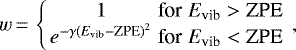$w = {\begin{matrix} 1 & for & E_{vib} > ZPE \\ e^{- γ {(E_{vib} - ZPE)}^{2}} & for & E_{vib} < ZPE \end{matrix},$ $\begin{eqnarray*} w\,{=}\,\left\lbrace \begin{array}{ccc} 1 &\textrm{for} & E_{\textrm{vib}} > \textrm{ZPE}\\ e^{-\gamma (E_{\textrm{vib}}-\textrm{ZPE})^2} & \textrm{for} & E_{\textrm{vib}} < \textrm{ZPE} \end{array} \right. , \end{eqnarray*}$ (A.5)

where E_vib is the vibrational energy of reactants (adding those of H₂ and SH⁺) or H₂ S⁺ products at the end of each trajectory. These new weights are used to calculate N_r and N_tot in Eq. (tabfloatlinking A.4). ZPE-corrected results are shown in Fig. A.3 with open symbols. This plot shows that all values are nearly the same as those calculated simply by counting trajectories as an integer (as done in the normal binning method; see filled symbols in Fig. A.3). The only exception is the case of SH⁺ + H₂ (v = 1) below 400 meV, which becomes zero when considering the ZPE of fragments at the end of the trajectories.

The reaction thermal rate in specific initial vibrational state of reactants are calculated running a minimum of 10⁵ trajectories per temperature, with fixed vibrational states of reactants, assuming a Boltzmann distribution over translational and rotational degrees of freedom, and following the ZPE-corrected method as: 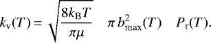$k_{v} (T) = \sqrt{\frac{8 k_{B} T}{π μ}} π b_{max}^{2} (T) P_{r} (T) .$ $\begin{eqnarray*}k_{\textrm{v}}(T)\,{=}\, \sqrt{{8 k_{\textrm{B}} T\over \pi\mu}}\quad \pi \, b^2_{\textrm{max}}(T)\quad P_{\textrm{r}}(T). \end{eqnarray*}$ (A.6)

The results of these calculations are shown in Fig. A.1. A.3:

A.3 On the radiative associations of H_n S⁺

Herbst et al. (1989) and Millar & Herbst (1990) proposed that the radiative association H_nS⁺ + H₂ → H_n+1S⁺ + hν is viable process at low gas temperatures. Although this chemical route is widely used in astrochemical models, here we question the viability of this process. The lower multiplicity (L) PESs of H₂ S⁺ (²A″) and H₃ S⁺ (¹A) are L = 1/2 and 0 respectively. These are shown in Fig. 9, together with the minimum multiplicity electronic state of H₄ S⁺ (bottom panel). This state does not have a deep well or any higher multiplicity state that could connect to higher states of reactants and products.

For of H₃ S⁺ formation through radiative association, this process assumes that a H₃ S $^{+} (^{3} A)$ $^+(^3A)$ ^* complex forms in a triplet state, the high spin state H considered here. According to our calculations, such a complex is formed after low-energy H₂ (v = 0, 1) + SH⁺ reactions (below 40 meV). The complex is formed in the ³W₁ well, corresponding to geometries very far from those of the low spin well, the ¹ W well. Therefore, a radiative spin flip and decay through phosphorescence is not possible. Herbst et al. (1989) proposed a second step, in which the spin flips from the triplet to the singlet state, followed by a radiative association, finally leading to the H₃ S $^{+} (^{1} A)$ $^+(^1A)$ product.

The origin of the spin flip must be the spin-orbit couplings, very relevant for S-bearing species, that favor the spin transition when singlet and triplet states are close in energy. Using the PESs calculated here, the lowest crossing region is at ≃ 0.25 eV, very close to that of H₂ (v = 0). At low temperatures, the H₃ S $^{+} (^{3} A)$ $^+(^3A)$ ^* complex formed by H₂ (v = 0) + SH⁺ reactions might allow a transition between the two electronic states with different spin. However, the spin flip probability is proportional to the square of the overlap $| 〈 H_{3} S^{+} {(^{3} A)}^{*} | H_{3} S^{+} {(^{1} A)}^{*} 〉 |^{2}$ $\vert\langle {\textrm{H}_3\textrm{S}^+}\,(^3A)^* \,\vert \,{\textrm{H}_3\textrm{S}^+}\,(^1A)^*\rangle \vert^2$ . This probability is very small because the two wells, ³W₁ and ¹W₁, correspond to very different geometries. In consequence, we conclude that this radiative association mechanism must be negligible, especially at the high gas temperatures of PDR edges where the H₃ S⁺(³A)^* complex is not formed.

As an alternative, a spin flip in a direct collision (not forming a H₃ S $^{+} {(^{3} A)}^{*}$ $^+(^3A)^*$ complex) may be more efficient and should be further investigated. Indeed, experimental measurements of the S $^{+} (^{4} S)$ $^+(^4S)$ + H₂ (v = 0) cross section show a maximum at about 1 eV of collisional energy attributed to spin-orbit transitions leading to spin flip (Stowe et al. 1990).

Appendix B Reaction S (³P) + H₂ (v) ⇄ SH + H

This reaction involves open shell reactants, S (³P), and products, SH (²Π). Neglecting spin flipping, there are three states that correlate to S(³ P), two of them connect to the SH (²Π). These two electronic states are of ³A′ and ³A″ symmetry, and have been studied in detail by Maiti et al. (2004). Here we use the adiabatic PES calculated by Maiti et al. (2004). Reaction S + H₂ → SH + H is endothermic by ≃1.02 eV (without zero-point energy corrections), very similar to the endothermicity of reaction S⁺ + H₂ → SH⁺ + H (Zanchet et al. 2013a, 2019). The main difference is the presence of a barrier, of ≃78 meV (≃905 K) with respect to the SH + H asymptote.

We performed quantum wave packet calculations for the reactions S + H₂ (v = 2, 3, j = 0) and SH (v = 0, j = 0) + H. We used MADWAVE3 (Gómez-Carrasco & Roncero 2006; Zanchet et al. 2009) to calculate the reaction probabilities for the initial vibrational state of the diatomic reactant (in the ground state rotational state, j = 0). We employed the usual partial wave expansion to calculate the reaction cross section. We calculated only few total angular momenta of the triatomic system, J = 0, 10 and 20. The other J needed in the partial wave expansion were obtained using the J-shifting-interpolation method (see Zanchet et al. 2013a). The initial-state-specific rate constants are obtained by numerical integration of the cross section using a Boltzmann distribution (Zanchet et al. 2013a). The resulting reaction rate constants are shown in Figs. B.1 and B.2. The numerical values of the rate constants are fitted to the usual analytical Arrhenius-like expresion (shown as dotted curves). We note that the shoulder in the rate constants of reaction SH (v = 0) + H requires two functions in the temperature range of 200–800 K. Rate coefficients are tabulated in Table 1.

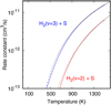Fig. B.1

Calculated rate constants as a function of temperature for reaction S(³ P) + H₂(v) → SH + H. Dotted curves are fits of the form k(T) = α (T/300)^β exp(−γ∕T). Rate coefficients are listed in Table 1.

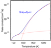Fig. B.2

Calculated rate constants as a function of temperature for reaction SH (v = 0) + H → S + H₂. The best fitto the calculated rate requires two Arrhenius-like expressions (one for low temperatures and one for high temperatures). Rate coefficients of these fits are listed in Table 1.

Appendix C SH and H₂S photoionization and photodissociation cross sections

Figure C.1 shows the experimental SH and H₂ S photoionization and photodissociation cross sections (cm⁻²) used in our PDR models. We integrate these cross sections over the specific FUV radiation field at each A_V depth of the PDR to obtain the specific photoionization and photodissociation rates (s⁻¹).

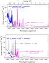Fig. C.1

Photoionization and photodissociation cross sections. Top panel: σ_ion(SH) (blue curve from laboratory experiments by Hrodmarsson et al. 2019). The pink curve is σ_diss (SH) (Heays et al. 2017, and references therein). Bottom panel: σ_ion(H₂S) (blue curve) and σ_diss(H₂S) (gray and pink curves; from Zhou et al. 2020).

Appendix D H₂S ortho-to-para ratio and T_spin

The OTP ratio is sometimes related to a nuclear-spin-temperature (T_spin, e.g., Mumma et al. 1987)defined, for H₂O or H₂S, as: 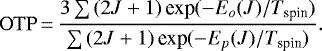$OTP = \frac{3 \sum (2 J + 1) exp (- E_{o} (J) / T_{spin})}{\sum (2 J + 1) exp (- E_{p} (J) / T_{spin})} .$ $\begin{equation*}{{\rm{OTP}}\,{=}\,\frac{3\sum{(2J+1)\,\textrm{{exp}}(-E_o(J)/T_{\textrm{spin}})}}{\sum{(2J+1)\,\textrm{{exp}}(-E_p(J)/T_{\textrm{spin}})}}}. \end{equation*}$ (D.1)

Here, E_o(J) and E_p (J) are the energies (in Kelvin) of o-H₂S and p-H₂S rotational levels (with the two ground rotational states separated by ΔE = 19.8 K). Figure D.1shows the OTP ratio of the two H₂S nuclear spin isomers as a function of T_spin. The OTP ratio we infer toward the DF position of the Bar, 2.9 ± 0.3, is consistent with the statistical ratio of 3/1, and implies T_spin ≥ 30 ± 10 K.

Fig. D.1

OTP ratio of H₂S as a function of spin temperature (Eq. (D.1)).

Appendix E Line parameters of IRAM 30 m, ALMA, and SOFIA observations

Table E.1

Parameters of H₂S and H $_{2}^{34}$ $_{2}^{34}$ S lines detected with the IRAM 30 m telescope toward three positions of the Orion Bar.

Table E.2

Parameters of SH⁺ targeted with ALMA toward the DF position.

Table E.3

Parameters of SH lines (neglecting HFS) targeted with SOFIA toward the DF position.

References

Aguado, A., & Paniagua, M. 1992, J. Chem. Phys., 96, 1265 [NASA ADS] [CrossRef] [Google Scholar]
Aguado, A., Tablero, C., & Paniagua, M. 2001, Comput. Phys. Comm., 134, 97 [NASA ADS] [CrossRef] [Google Scholar]
Aguado, A., Barragan, P., Prosmiti, R., et al. 2010, J. Chem. Phys., 133, 024306 [NASA ADS] [CrossRef] [Google Scholar]
Agúndez, M., & Wakelam, V. 2013, Chemical Reviews, 113, 8710 [Google Scholar]
Agúndez, M., Goicoechea, J. R., Cernicharo, J., Faure, A., & Roueff, E. 2010, ApJ, 713, 662 [NASA ADS] [CrossRef] [Google Scholar]
Allers, K. N., Jaffe, D. T., Lacy, J. H., Draine, B. T., & Richter, M. J. 2005, ApJ, 630, 368 [NASA ADS] [CrossRef] [Google Scholar]
Anders, E., & Grevesse, N. 1989, Geochim. Cosmochim. Acta, 53, 197 [Google Scholar]
Andree-Labsch, S., Ossenkopf-Okada, V., & Röllig, M. 2017, A&A, 598, A2 [NASA ADS] [CrossRef] [EDP Sciences] [Google Scholar]
Anicich, V. G. 2003, An Index Of The Literature For Bimolecular Gas Phase Cation-Molecule Reaction Kinetics (California: JPL Publication), 1 [Google Scholar]
Arab, H., Abergel, A., Habart, E., et al. 2012, A&A, 541, A19 [NASA ADS] [CrossRef] [EDP Sciences] [Google Scholar]
Asplund, M., Grevesse, N., Sauval, A. J., & Scott, P. 2009, ARA&A, 47, 481 [NASA ADS] [CrossRef] [Google Scholar]
Azzam, A. A. A., Yurchenko, S. N., Tennyson, J., Martin-Drumel, M.-A., & Pirali, O. 2013, J. Quant. Spectr. Rad. Transf., 130, 341 [NASA ADS] [CrossRef] [Google Scholar]
Badnell, N. R. 1991, ApJ, 379, 356 [NASA ADS] [CrossRef] [Google Scholar]
Bally, J. 2008, Overview of the Orion Complex, ed. B. Reipurth (USA: Nasa), 459 [Google Scholar]
Bañares, L., Aoiz, F. J., Honvault, P., Bussery-Honvault, B., & Launay, J.-M. 2003, J. Chem. Phys., 118, 565 [Google Scholar]
Bañares, L., Aoiz, F. J., Honvault, P., & Launay, J.-M. 2004, J. Phys. Chem., 108, 1616 [Google Scholar]
Black, J. H. 1998, Faraday Discuss., 109, 257 [NASA ADS] [CrossRef] [Google Scholar]
Bonnet, L., & Rayez, J.-C. 1997, Chem. Phys. Lett., 277, 183 [NASA ADS] [CrossRef] [Google Scholar]
Bonnet, L., & Rayez, J.-C. 2004, Chem. Phys. Lett., 397, 106 [NASA ADS] [CrossRef] [Google Scholar]
Brittain, A., Coolbroth, K., & Boogert, A. 2020, AAS Meeting Abstracts, 236, 247.08 [NASA ADS] [Google Scholar]
Bron, E., Le Bourlot, J., & Le Petit, F. 2014, A&A, 569, A100 [NASA ADS] [CrossRef] [EDP Sciences] [Google Scholar]
Bron, E., Agúndez, M., Goicoechea, J. R., & Cernicharo, J. 2018, ArXiv eprints [arXiv:1801.01547] [Google Scholar]
Buckinghan, A. D. 1967, Adv. Chem. Phys., 12, 107 [CrossRef] [Google Scholar]
Burton, M. G., Hollenbach, D. J., & Tielens, A. G. G. M. 1990, ApJ, 365, 620 [NASA ADS] [CrossRef] [Google Scholar]
Calmonte, U., Altwegg, K., Balsiger, H., et al. 2016, MNRAS, 462, S253 [CrossRef] [Google Scholar]
Cardelli, J. A., Clayton, G. C., & Mathis, J. S. 1989, ApJ, 345, 245 [NASA ADS] [CrossRef] [Google Scholar]
Caselli, P., Keto, E., Pagani, L., et al. 2010, A&A, 521, L29 [NASA ADS] [CrossRef] [EDP Sciences] [Google Scholar]
Caselli, P., Keto, E., Bergin, E. A., et al. 2012, ApJ, 759, L37 [Google Scholar]
Charnley, S. B. 1997, ApJ, 481, 396 [NASA ADS] [CrossRef] [Google Scholar]
Choi, Y., van der Tak, F. F. S., Bergin, E. A., & Plume, R. 2014, A&A, 572, L10 [Google Scholar]
Collings, M. P., Anderson, M. A., Chen, R., et al. 2004, MNRAS, 354, 1133 [NASA ADS] [CrossRef] [Google Scholar]
Crockett, N. R., Bergin, E. A., Neill, J. L., et al. 2014, ApJ, 781, 114 [NASA ADS] [CrossRef] [Google Scholar]
Cruz-Diaz, G. A., Muñoz Caro, G. M., Chen, Y. J., & Yih, T. S. 2014, A&A, 562, A119 [NASA ADS] [CrossRef] [EDP Sciences] [Google Scholar]
Cuadrado, S., Goicoechea, J. R., Pilleri, P., et al. 2015, A&A, 575, A82 [NASA ADS] [CrossRef] [EDP Sciences] [Google Scholar]
Cuadrado, S., Goicoechea, J. R., Roncero, O., et al. 2016, A&A, 596, L1 [NASA ADS] [CrossRef] [EDP Sciences] [Google Scholar]
Cuadrado, S., Goicoechea, J. R., Cernicharo, J., et al. 2017, A&A, 603, A124 [NASA ADS] [CrossRef] [EDP Sciences] [Google Scholar]
Cuadrado, S., Salas, P., Goicoechea, J. R., et al. 2019, A&A, 625, L3 [CrossRef] [EDP Sciences] [Google Scholar]
Dagdigian, P. J. 2019a, MNRAS, 487, 3427 [CrossRef] [Google Scholar]
Dagdigian, P. J. 2019b, J. Chem. Phys., 150, 084308 [CrossRef] [Google Scholar]
Dagdigian, P. J. 2020, MNRAS, 494, 5239 [NASA ADS] [CrossRef] [Google Scholar]
Dartois, E. 2005, Space Sci. Rev., 119, 293 [NASA ADS] [CrossRef] [Google Scholar]
Davidson, E. R. 1975, J. Comp. Phys., 17, 87 [NASA ADS] [CrossRef] [MathSciNet] [Google Scholar]
de Graauw, T., Helmich, F. P., Phillips, T. G., et al. 2010, A&A, 518, L6 [NASA ADS] [CrossRef] [EDP Sciences] [Google Scholar]
Desrousseaux, B., Lique, F., Goicoechea, J. R., Quintas-Sánchez, E., & Dawes, R. 2021, A&A, 645, A8 [NASA ADS] [CrossRef] [EDP Sciences] [Google Scholar]
Endres, C. P., Schlemmer, S., Schilke, P., Stutzki, J., & Müller, H. S. P. 2016, J. Mol. Spectr., 327, 95 [NASA ADS] [CrossRef] [Google Scholar]
Esplugues, G. B., Viti, S., Goicoechea, J. R., & Cernicharo, J. 2014, A&A, 567, A95 [NASA ADS] [CrossRef] [EDP Sciences] [Google Scholar]
Esplugues, G. B., Cazaux, S., Meijerink, R., Spaans, M., & Caselli, P. 2016, A&A, 591, A52 [NASA ADS] [CrossRef] [EDP Sciences] [Google Scholar]
Farah, K., Muller-Plathe, F., & Bohm, M. C. 2012, Chem. Phys. Chem., 13, 1127 [Google Scholar]
Faure, A., Halvick, P., Stoecklin, T., et al. 2017, MNRAS, 469, 612 [NASA ADS] [CrossRef] [Google Scholar]
Freeman, A., & Williams, D. A. 1982, Ap&SS, 83, 417 [CrossRef] [Google Scholar]
Fuente, A., Rodrıguez-Franco, A., Garcıa-Burillo, S., Martın-Pintado, J., & Black, J. H. 2003, A&A, 406, 899 [NASA ADS] [CrossRef] [EDP Sciences] [Google Scholar]
Fuente, A., Cernicharo, J., Roueff, E., et al. 2016, A&A, 593, A94 [NASA ADS] [CrossRef] [EDP Sciences] [Google Scholar]
Fuente, A., Goicoechea, J. R., Pety, J., et al. 2017, ApJ, 851, L49 [NASA ADS] [CrossRef] [Google Scholar]
Fuente, A., Navarro, D. G., Caselli, P., et al. 2019, A&A, 624, A105 [NASA ADS] [CrossRef] [EDP Sciences] [Google Scholar]
Garrod, R. T., Wakelam, V., & Herbst, E. 2007, A&A, 467, 1103 [NASA ADS] [CrossRef] [EDP Sciences] [Google Scholar]
Genzel, R., & Stutzki, J. 1989, ARA&A, 27, 41 [NASA ADS] [CrossRef] [Google Scholar]
Gerin, M., de Luca, M., Black, J., et al. 2010, A&A, 518, L110 [NASA ADS] [CrossRef] [EDP Sciences] [Google Scholar]
Gerin, M., Neufeld, D. A., & Goicoechea, J. R. 2016, ARA&A, 54, 181 [NASA ADS] [CrossRef] [Google Scholar]
Gibb, E. L., Whittet, D. C. B., Boogert, A. C. A., & Tielens, A. G. G. M. 2004, ApJS, 151, 35 [NASA ADS] [CrossRef] [PubMed] [Google Scholar]
Godard, B., & Cernicharo, J. 2013, A&A, 550, A8 [NASA ADS] [CrossRef] [EDP Sciences] [Google Scholar]
Godard, B., Falgarone, E., Gerin, M., et al. 2012, A&A, 540, A87 [NASA ADS] [CrossRef] [EDP Sciences] [Google Scholar]
Godard, B., Falgarone, E., & Pineau des Forêts, G. 2014, A&A, 570, A27 [NASA ADS] [CrossRef] [EDP Sciences] [Google Scholar]
Goicoechea, J. R., & Le Bourlot, J. 2007, A&A, 467, 1 [NASA ADS] [CrossRef] [EDP Sciences] [Google Scholar]
Goicoechea, J. R., Pety, J., Gerin, M., et al. 2006, A&A, 456, 565 [NASA ADS] [CrossRef] [EDP Sciences] [Google Scholar]
Goicoechea, J. R., Pety, J., Gerin, M., Hily-Blant, P., & Le Bourlot, J. 2009, A&A, 498, 771 [NASA ADS] [CrossRef] [EDP Sciences] [Google Scholar]
Goicoechea, J. R., Joblin, C., Contursi, A., et al. 2011, A&A, 530, L16 [NASA ADS] [CrossRef] [EDP Sciences] [Google Scholar]
Goicoechea, J. R., Cernicharo, J., Karska, A., et al. 2012, A&A, 548, A77 [NASA ADS] [CrossRef] [EDP Sciences] [Google Scholar]
Goicoechea, J. R., Pety, J., Cuadrado, S., et al. 2016, Nature, 537, 207 [NASA ADS] [CrossRef] [Google Scholar]
Goicoechea, J. R., Cuadrado, S., Pety, J., et al. 2017, A&A, 601, L9 [NASA ADS] [CrossRef] [EDP Sciences] [Google Scholar]
Goicoechea, J. R., Santa-Maria, M. G., Bron, E., et al. 2019, A&A, 622, A91 [NASA ADS] [CrossRef] [EDP Sciences] [Google Scholar]
Goicoechea, J. R., Pabst, C. H. M., Kabanovic, S., et al. 2020, A&A, 639, A1 [CrossRef] [EDP Sciences] [Google Scholar]
Gómez-Carrasco, S., & Roncero, O. 2006, J. Chem. Phys., 125, 054102 [NASA ADS] [CrossRef] [PubMed] [Google Scholar]
Graedel, T. E., Langer, W. D., & Frerking, M. A. 1982, ApJS, 48, 321 [NASA ADS] [CrossRef] [Google Scholar]
Grozdanov, T. P., & Solov’ev, E. A. 1982, J. Phys. B, 15, 1195 [CrossRef] [Google Scholar]
Guzmán, V. V., Goicoechea, J. R., Pety, J., et al. 2013, A&A, 560, A73 [NASA ADS] [CrossRef] [EDP Sciences] [Google Scholar]
Habart, E., Dartois, E., Abergel, A., et al. 2010, A&A, 518, L116 [NASA ADS] [CrossRef] [EDP Sciences] [Google Scholar]
Habing, H. J. 1968, Bull. Astron. Inst. Netherlands, 19, 421 [Google Scholar]
Hama, T., Kouchi, A., & Watanabe, N. 2016, Science, 351, 65 [NASA ADS] [CrossRef] [Google Scholar]
Hamilton, J. R., Faure, A., & Tennyson, J. 2018, MNRAS, 476, 2931 [NASA ADS] [CrossRef] [Google Scholar]
Hasegawa, T. I., & Herbst, E. 1993, MNRAS, 261, 83 [NASA ADS] [CrossRef] [Google Scholar]
Hatchell, J., Thompson, M. A., Millar, T. J., & MacDonald, G. H. 1998, A&A, 338, 713 [Google Scholar]
He, J., Shi, J., Hopkins, T., Vidali, G., & Kaufman, M. J. 2015, ApJ, 801, 120 [NASA ADS] [CrossRef] [Google Scholar]
Heays, A. N., Bosman, A. D., & van Dishoeck, E. F. 2017, A&A, 602, A105 [NASA ADS] [CrossRef] [EDP Sciences] [Google Scholar]
Heikkilä, A., Johansson, L. E. B., & Olofsson, H. 1999, A&A, 344, 817 [NASA ADS] [Google Scholar]
Herbst, E., DeFrees, D. J., & Koch, W. 1989, MNRAS, 237, 1057 [NASA ADS] [CrossRef] [Google Scholar]
Herpin, F., Marseille, M., Wakelam, V., Bontemps, S., & Lis, D. C. 2009, A&A, 504, 853 [NASA ADS] [CrossRef] [EDP Sciences] [Google Scholar]
Heyminck, S., Graf, U. U., Güsten, R., et al. 2012, A&A, 542, L1 [NASA ADS] [CrossRef] [EDP Sciences] [Google Scholar]
Hogerheijde, M. R., Jansen, D. J., & van Dishoeck, E. F. 1995, A&A, 294, 792 [NASA ADS] [Google Scholar]
Holdship, J., Jimenez-Serra, I., Viti, S., et al. 2019, ApJ, 878, 64 [NASA ADS] [CrossRef] [Google Scholar]
Hollenbach, D. J., & Tielens, A. G. G. M. 1997, ARA&A, 35, 179 [NASA ADS] [CrossRef] [Google Scholar]
Hollenbach, D., Kaufman, M. J., Bergin, E. A., & Melnick, G. J. 2009, ApJ, 690, 1497 [CrossRef] [Google Scholar]
Hollenbach, D., Kaufman, M. J., Neufeld, D., Wolfire, M., & Goicoechea, J. R. 2012, ApJ, 754, 105 [NASA ADS] [CrossRef] [Google Scholar]
Hosokawa, T., & Inutsuka, S.-i. 2006, ApJ, 646, 240 [NASA ADS] [CrossRef] [Google Scholar]
Howk, J. C., Sembach, K. R., & Savage, B. D. 2006, ApJ, 637, 333 [NASA ADS] [CrossRef] [Google Scholar]
Hrodmarsson, H. R., Garcia, G. A., Nahon, L., Loison, J.-C., & Gans, B. 2019, Physi. Chem. Chem. Phys., 21, 25907 [NASA ADS] [CrossRef] [Google Scholar]
Indriolo, N., Neufeld, D. A., Gerin, M., et al. 2015, ApJ, 800, 40 [NASA ADS] [CrossRef] [Google Scholar]
Ioppolo, S., Cuppen, H. M., Romanzin, C., van Dishoeck, E. F., & Linnartz, H. 2008, ApJ, 686, 1474 [NASA ADS] [CrossRef] [Google Scholar]
Jansen, D. J., Spaans, M., Hogerheijde, M. R., & van Dishoeck, E. F. 1995, A&A, 303, 541 [NASA ADS] [Google Scholar]
Jiménez-Escobar, A., & Muñoz Caro, G. M. 2011, A&A, 536, A91 [NASA ADS] [CrossRef] [EDP Sciences] [Google Scholar]
Jiménez-Serra, I., Zhang, Q., Viti, S., Martín-Pintado, J., & de Wit, W. J. 2012, ApJ, 753, 34 [NASA ADS] [CrossRef] [Google Scholar]
Joblin, C., Bron, E., Pinto, C., et al. 2018, A&A, 615, A129 [NASA ADS] [CrossRef] [EDP Sciences] [Google Scholar]
Johnson, B. R. 1987, J. Chem. Phys., 86, 1445 [NASA ADS] [CrossRef] [Google Scholar]
Kaplan, K. F., Dinerstein, H. L., Oh, H., et al. 2017, ApJ, 838, 152 [NASA ADS] [CrossRef] [Google Scholar]
Karplus, M., Porter, R. N., & Sharma, R. D. 1965, J. Chem. Phys., 43, 3259 [NASA ADS] [CrossRef] [Google Scholar]
Kirsanova, M. S., & Wiebe, D. S. 2019, MNRAS, 486, 2525 [CrossRef] [Google Scholar]
Klisch, E., Klaus, T., Belov, S. P., et al. 1996, ApJ, 473, 1118 [NASA ADS] [CrossRef] [Google Scholar]
Kłos, J., Lique, F., & Alexander, M. H. 2009, Chem. Phys. Lett., 476, 135 [NASA ADS] [CrossRef] [Google Scholar]
Knizia, G., Adler, T. B., & Werner, H. J. 2009, J. Chem. Phys., 130, 054104 [NASA ADS] [CrossRef] [Google Scholar]
Laas, J. C., & Caselli, P. 2019, A&A, 624, A108 [CrossRef] [EDP Sciences] [Google Scholar]
Le Bourlot, J., Le Petit, F., Pinto, C., Roueff, E., & Roy, F. 2012, A&A, 541, A76 [NASA ADS] [CrossRef] [EDP Sciences] [Google Scholar]
Lee, T. A. 1968, ApJ, 152, 913 [NASA ADS] [CrossRef] [Google Scholar]
Le Petit, F., Nehmé, C., Le Bourlot, J., & Roueff, E. 2006, ApJS, 164, 506 [NASA ADS] [CrossRef] [EDP Sciences] [Google Scholar]
Leurini, S., Rolffs, R., Thorwirth, S., et al. 2006, A&A, 454, L47 [NASA ADS] [CrossRef] [EDP Sciences] [Google Scholar]
Levine, R. D., & Bernstein, R. B. 1987, Mol Reaction Dynamics and Chemical Reactivity (Oxford: Oxford University Press) [Google Scholar]
Lique, F., Zanchet, A., Bulut, N., Goicoechea, J. R., & Roncero, O. 2020, A&A, 638, A72 [NASA ADS] [CrossRef] [EDP Sciences] [Google Scholar]
Lis, D. C., Bergin, E. A., Schilke, P., & van Dishoeck, E. F. 2013, J. Phys. Chem. A, 117, 9661 [CrossRef] [Google Scholar]
Lucas, R., & Liszt, H. S. 2002, A&A, 384, 1054 [NASA ADS] [CrossRef] [EDP Sciences] [Google Scholar]
Maiti, B., Schatz, G. C., & Lendvay, G. 2004, J. Phys. Chem. A, 108, 8772 [NASA ADS] [CrossRef] [Google Scholar]
Marconi, A., Testi, L., Natta, A., & Walmsley, C. M. 1998, A&A, 330, 696 [NASA ADS] [Google Scholar]
Martín, S., Mauersberger, R., Martín-Pintado, J., Henkel, C., & García-Burillo, S. 2006, ApJS, 164, 450 [NASA ADS] [CrossRef] [Google Scholar]
Martín, S., Krips, M., Martín-Pintado, J., et al. 2011, A&A, 527, A36 [NASA ADS] [CrossRef] [EDP Sciences] [Google Scholar]
Martin-Drumel, M. A., Eliet, S., Pirali, O., et al. 2012, Chem. Phys. Lett., 550, 8 [CrossRef] [Google Scholar]
Melnick, G. J., Tolls, V., Goldsmith, P. F., et al. 2012, ApJ, 752, 26 [NASA ADS] [CrossRef] [Google Scholar]
Melnick, G. J., Tolls, V., Snell, R. L., et al. 2020, ApJ, 892, 22 [CrossRef] [Google Scholar]
Menten, K. M., Wyrowski, F., Belloche, A., et al. 2011, A&A, 525, A77 [NASA ADS] [CrossRef] [EDP Sciences] [Google Scholar]
Millar, T. J., & Herbst, E. 1990, A&A, 231, 466 [NASA ADS] [Google Scholar]
Millar, T. J., Adams, N. G., Smith, D., Lindinger, W., & Villinger, H. 1986, MNRAS, 221, 673 [NASA ADS] [CrossRef] [Google Scholar]
Minissale, M., & Dulieu, F. 2014, J. Chem. Phys., 141, 014304 [NASA ADS] [CrossRef] [Google Scholar]
Minissale, M., Dulieu, F., Cazaux, S., & Hocuk, S. 2016, A&A, 585, A24 [NASA ADS] [CrossRef] [EDP Sciences] [Google Scholar]
Mumma, M. J., Weaver, H. A., & Larson, H. P. 1987, A&A, 187, 419 [NASA ADS] [Google Scholar]
Nagy, T., & Lendvay, G. 2017, J. Phys. Chem. Lett., 8, 4621 [CrossRef] [Google Scholar]
Nagy, Z., Van der Tak, F. F. S., Ossenkopf, V., et al. 2013, A&A, 550, A96 [NASA ADS] [CrossRef] [EDP Sciences] [Google Scholar]
Nagy, Z., Choi, Y., Ossenkopf-Okada, V., et al. 2017, A&A, 599, A22 [NASA ADS] [CrossRef] [EDP Sciences] [Google Scholar]
Navarro-Almaida, D., Le Gal, R., Fuente, A., et al. 2020, A&A, 637, A39 [CrossRef] [EDP Sciences] [Google Scholar]
Neufeld, D. A., Nisini, B., Giannini, T., et al. 2009, ApJ, 706, 170 [NASA ADS] [CrossRef] [Google Scholar]
Neufeld, D. A., Goicoechea, J. R., Sonnentrucker, P., et al. 2010, A&A, 521, L10 [NASA ADS] [CrossRef] [EDP Sciences] [Google Scholar]
Neufeld, D. A., Falgarone, E., Gerin, M., et al. 2012, A&A, 542, L6 [NASA ADS] [CrossRef] [EDP Sciences] [Google Scholar]
Neufeld, D. A., Godard, B., Gerin, M., et al. 2015, A&A, 577, A49 [NASA ADS] [CrossRef] [EDP Sciences] [Google Scholar]
Oba, Y., Tomaru, T., Lamberts, T., Kouchi, A., & Watanabe, N. 2018, Nat. Astron., 2, 228 [NASA ADS] [CrossRef] [Google Scholar]
O’Dell, C. R. 2001, ARA&A, 39, 99 [NASA ADS] [CrossRef] [Google Scholar]
Pabst, C., Higgins, R., Goicoechea, J. R., et al. 2019, Nature, 565, 618 [NASA ADS] [CrossRef] [Google Scholar]
Pabst, C. H. M., Goicoechea, J. R., Teyssier, D., et al. 2020, A&A, 639, A2 [CrossRef] [EDP Sciences] [Google Scholar]
Palumbo, M. E., Geballe, T. R., & Tielens, A. G. G. M. 1997, ApJ, 479, 839 [NASA ADS] [CrossRef] [Google Scholar]
Pankonin, V., & Walmsley, C. M. 1978, A&A, 64, 333 [NASA ADS] [Google Scholar]
Parikka, A., Habart, E., Bernard-Salas, J., et al. 2017, A&A, 599, A20 [NASA ADS] [CrossRef] [EDP Sciences] [Google Scholar]
Pellegrini, E. W., Baldwin, J. A., Ferland, G. J., Shaw, G., & Heathcote, S. 2009, ApJ, 693, 285 [NASA ADS] [CrossRef] [Google Scholar]
Peterson, K. A., Adler, T. B., & Werner, H. J. 2008, J. Chem. Phys., 128, 084102 [NASA ADS] [CrossRef] [Google Scholar]
Pineau des Forets, G., Flower, D. R., Hartquist, T. W., & Dalgarno, A. 1986, MNRAS, 220, 801 [NASA ADS] [CrossRef] [Google Scholar]
Prasad, S. S., & Huntress, W. T., J. 1980, ApJS, 43, 1 [NASA ADS] [CrossRef] [Google Scholar]
Prasad, S. S., & Huntress, W. T., J. 1982, ApJ, 260, 590 [NASA ADS] [CrossRef] [Google Scholar]
Putaud, T., Michaut, X., Le Petit, F., Roueff, E., & Lis, D. C. 2019, A&A, 632, A8 [NASA ADS] [CrossRef] [EDP Sciences] [Google Scholar]
Qu, C., & Bowman, J. M. 2016, J. Phys. Chem. A, 120, 4988 [CrossRef] [Google Scholar]
Rivière-Marichalar, P., Fuente, A., Goicoechea, J. R., et al. 2019, A&A, 628, A16 [NASA ADS] [CrossRef] [EDP Sciences] [Google Scholar]
Roelfsema, P. R., Helmich, F. P., Teyssier, D., et al. 2012, A&A, 537, A17 [NASA ADS] [CrossRef] [EDP Sciences] [Google Scholar]
Roncero, O., Zanchet, A., & Aguado, A. 2018, Phys. Chem. Chem. Phys., 20, 25951 [NASA ADS] [CrossRef] [Google Scholar]
Rosenthal, D., Bertoldi, F., & Drapatz, S. 2000, A&A, 356, 705 [NASA ADS] [Google Scholar]
Sandford, S. A., & Allamandola, L. J. 1988, Icarus, 76, 201 [NASA ADS] [CrossRef] [Google Scholar]
Sanz-Sanz, C., Roncero, O., Paniagua, M., & Aguado, A. 2013, J. Chem. Phys., 139, 184302 [NASA ADS] [CrossRef] [Google Scholar]
Shiozaki, T., & Werner, H.-J. 2013, Mol. Phys., 111, 607 [NASA ADS] [CrossRef] [Google Scholar]
Smirnov, G. T., Sorochenko, R. L., & Walmsley, C. M. 1995, A&A, 300, 923 [NASA ADS] [Google Scholar]
Smith, R. G. 1991, MNRAS, 249, 172 [NASA ADS] [CrossRef] [Google Scholar]
Sofia, U. J., Lauroesch, J. T., Meyer, D. M., & Cartledge, S. I. B. 2004, ApJ, 605, 272 [NASA ADS] [CrossRef] [Google Scholar]
Stecher, T. P., & Williams, D. A. 1972, ApJ, 177, L141 [NASA ADS] [CrossRef] [Google Scholar]
Sternberg, A., & Dalgarno, A. 1995, ApJS, 99, 565 [NASA ADS] [CrossRef] [Google Scholar]
Stoerzer, H., Stutzki, J., & Sternberg, A. 1995, A&A, 296, L9 [NASA ADS] [Google Scholar]
Stowe, G. F., Schultz, R. H., Wright, C. A., & Armentrout, P. B. 1990, Int. J. Mass Spectr. Ion Proc., 100, 377 [Google Scholar]
Tablero, C., Aguado, A., & Paniagua, M. 2001, Comput. Phys. Comm., 140, 412 [NASA ADS] [CrossRef] [Google Scholar]
Taquet, V., Furuya, K., Walsh, C., & van Dishoeck, E. F. 2016, MNRAS, 462, S99 [Google Scholar]
Tercero, B., Cernicharo, J., Pardo, J. R., & Goicoechea, J. R. 2010, A&A, 517, A96 [NASA ADS] [CrossRef] [EDP Sciences] [Google Scholar]
Tieftrunk, A., Pineau des Forets, G., Schilke, P., & Walmsley, C. M. 1994, A&A, 289, 579 [Google Scholar]
Tielens, A. G. G. M. 2010, The Physics and Chemistry of the Interstellar Medium (Cambridge: Cambridge University Press) [Google Scholar]
Tielens, A. G. G. M., & Hagen, W. 1982, A&A, 114, 245 [Google Scholar]
Tielens, A. G. G. M., & Hollenbach, D. 1985, ApJ, 291, 722 [Google Scholar]
Tielens, A. G. G. M., Meixner, M. M., van der Werf, P. P., et al. 1993, Science, 262, 86 [NASA ADS] [CrossRef] [PubMed] [Google Scholar]
Turner, B. E. 1996, ApJ, 468, 694 [NASA ADS] [CrossRef] [Google Scholar]
van der Tak, F. F. S., Boonman, A. M. S., Braakman, R., & van Dishoeck, E. F. 2003, A&A, 412, 133 [NASA ADS] [CrossRef] [EDP Sciences] [Google Scholar]
van der Tak, F. F. S., Black, J. H., Schöier, F. L., Jansen, D. J., & van Dishoeck, E. F. 2007, A&A, 468, 627 [NASA ADS] [CrossRef] [EDP Sciences] [Google Scholar]
van der Tak, F. F. S., Nagy, Z., Ossenkopf, V., et al. 2013, A&A, 560, A95 [NASA ADS] [CrossRef] [EDP Sciences] [Google Scholar]
van der Werf, P. P., Stutzki, J., Sternberg, A., & Krabbe, A. 1996, A&A, 313, 633 [NASA ADS] [Google Scholar]
van der Werf, P. P., Goss, W. M., & O’Dell, C. R. 2013, ApJ, 762, 101 [NASA ADS] [CrossRef] [Google Scholar]
van der Wiel, M. H. D., van der Tak, F. F. S., Ossenkopf, V., et al. 2009, A&A, 498, 161 [NASA ADS] [CrossRef] [EDP Sciences] [Google Scholar]
van Dishoeck, E. F. 2004, ARA&A, 42, 119 [NASA ADS] [CrossRef] [Google Scholar]
Velilla, L., Lepetit, B., Aguado, A., Beswick, J., & Paniagua, M. 2008, J. Chem. Phys., 129, 084307 [CrossRef] [PubMed] [Google Scholar]
Vidal, T. H. G., Loison, J.-C., Jaziri, A. Y., et al. 2017, MNRAS, 469, 435 [Google Scholar]
Wakelam, V., Loison, J. C., Mereau, R., & Ruaud, M. 2017, Mol. Astrophys., 6, 22 [NASA ADS] [CrossRef] [EDP Sciences] [Google Scholar]
Walmsley, C. M., Natta, A., Oliva, E., & Testi, L. 2000, A&A, 364, 301 [NASA ADS] [Google Scholar]
Werner, H. J., & Knowles, P. J. 1988a, J. Chem. Phys., 89, 5803 [NASA ADS] [CrossRef] [Google Scholar]
Werner, H. J., & Knowles, P. J. 1988b, Chem. Phys. Lett., 145, 514 [NASA ADS] [CrossRef] [Google Scholar]
Werner, H.-J., Knowles, P. J., Knizia, G., Manby, F. R., & Schütz, M. 2012, WIREs Comput. Mol. Sci., 2, 242 [CrossRef] [Google Scholar]
Wyrowski, F., Schilke, P., Hofner, P., & Walmsley, C. M. 1997, ApJ, 487, L171 [NASA ADS] [CrossRef] [Google Scholar]
Yamamura, I., Kawaguchi, K., & Ridgway, S. T. 2000, ApJ, 528, L33 [NASA ADS] [CrossRef] [Google Scholar]
Young, E. T., Becklin, E. E., Marcum, P. M., et al. 2012, ApJ, 749, L17 [NASA ADS] [CrossRef] [Google Scholar]
Zanchet, A., Roncero, O., González-Lezana, T., et al. 2009, J. Phys. Chem. A, 113, 14488 [CrossRef] [PubMed] [Google Scholar]
Zanchet, A., Agúndez, M., Herrero, V. J., Aguado, A., & Roncero, O. 2013a, AJ, 146, 125 [NASA ADS] [CrossRef] [Google Scholar]
Zanchet, A., Godard, B., Bulut, N., et al. 2013b, ApJ, 766, 80 [NASA ADS] [CrossRef] [Google Scholar]
Zanchet, A., del Mazo, P., Aguado, A., et al. 2018, PCCP, 20, 5415 [NASA ADS] [CrossRef] [Google Scholar]
Zanchet, A., Lique, F., Roncero, O., Goicoechea, J. R., & Bulut, N. 2019, A&A, 626, A103 [NASA ADS] [CrossRef] [EDP Sciences] [Google Scholar]
Zhou, J., Zhao, Y., Hansen, C. S., et al. 2020, Nat. Commun., 11, 1547 [NASA ADS] [CrossRef] [Google Scholar]

¹

SH was first reported by IR spectroscopy toward the cirumstellar envelope around the evolved star R Andromedae (Yamamura et al. 2000).

²

Sulfur has four stable isotopes, in decreasing order of abundance: ³²S (I_N = 0), ³⁴S (I_N = 0), ³³S (I_N = 3/2), and ³⁶S (I_N = 0), where I_N is the nuclear spin. The most abundant isotope is here simply referred to as S.

³

Readers interested only in the chemistry of these species and in depth-dependent PDR models could directly jump to Sect. 6.

⁴

We use the following inelastic collision rate coefficients γ_ij: • SH⁺– e⁻, including hyperfine splittings (Hamilton et al. 2018). • SH⁺– o-H₂ and p-H₂, including hyperfine splittings (Dagdigian 2019a). • SH⁺– H, including hyperfine splittings (Lique et al. 2020). • o-H₂S and p-H₂S with o-H₂ and p-H₂ (Dagdigian 2020). • SH– He, including fine-structure splittings (Kłos et al. 2009).

⁵

CH⁺ is more reactive than SH⁺ because CH⁺ does react with H₂ (v = 0) exothermically producing CH $_{2}^{+}$ $_{2}^{+}$ at k = 1.2 × 10⁻⁹ cm³ s⁻¹ (Anicich 2003) and also because reaction of CH⁺ with H is faster, k = 7.5 × 10⁻¹⁰ cm³ s⁻¹.

⁶

If one considers H₂ rovibrational levels, reaction (1) becomes exoergic for v = 0, J ≥ 11 and for v = 1, J ≥ 7 (Zanchet et al. 2019).

⁷

Older gas-phase PDR models previously predicted low H₂ S column densities (Jansen et al. 1995; Sternberg & Dalgarno 1995).

⁸

We only consider the depletion of neutral S atoms. S⁺ ions are expected to be more abundant than S atoms at the edge of the Orion Bar (A_V ≲ 2 mag) where T_k and T_d are too high, and the FUV radiation field too strong, to allow the formation of abundant grain mantles.

⁹

Crockett et al. (2014) inferred N(o-H₂S)/N(p-H₂S) = 2.5 ± 0.8 in the hot core of Orion KL using LTE rotational digrams. However, they favored an OTP ratio of 1.7 ± 0.8 based on the column density ratio of selected pairs of rotational levels with similar energies. This latter OTP ratio implies T_spin(H₂S) ≃ 12 K (Fig. D.1), perhaps related to much colder dust grains than in PDRs or to colder gas conditions just before the hot core phase; so that reactive collisions did not have time to establish the statistical equilibrium value. The observed OTP ratios of H₂ CO, H₂ CS, and H₂ CCO in the Bar are also ~3 (Cuadrado et al. 2017).

¹⁰

In these models we consider undepleted [S/H] abundances and only the chemical desorption s-H + s-SH → H₂S (with a 50% efficiency).

All Tables

Table 1

Relevant rate coefficients from a fit of the Arrhenius-like form k (T) = $α {(T / 300 K)}^{β} exp (- γ / T)$ $\alpha\,(T/300\,\textrm{K})^{\beta} \,\textrm{exp}(-\gamma/T)$ to the calculated reaction rates.

In the text

Table 2

Main parameters used in the PDR models of the Orion Bar.

In the text

Table 3

Column density predictions from different PDR models (up to A_V = 10 mag) and estimated values from observations (single-slab approach).

In the text

Table 4

Adopted binding energies and photodesorption yields.

In the text

Table A.1

RCCSD(T)-F12a and fit stationary points on the PES.

In the text

Table A.2

E_v of reactants and products, and adiabatic switching energies for the QCT initial conditions.

In the text

Table E.1

Parameters of H₂S and H $_{2}^{34}$ $_{2}^{34}$ S lines detected with the IRAM 30 m telescope toward three positions of the Orion Bar.

In the text

Table E.2

Parameters of SH⁺ targeted with ALMA toward the DF position.

In the text

Table E.3

Parameters of SH lines (neglecting HFS) targeted with SOFIA toward the DF position.

In the text

All Figures

Fig. 1

Overview of the Orion Bar. The (0″, 0″) position corresponds to α₂₀₀₀ = 05^h 35^m 20.1^s ; δ₂₀₀₀ = -05°25′07.0″. Left panel: integrated line intensity maps in the ¹³CO J = 3–2 (color scale) and SO 8₉–7₈ emission (gray contours; from 6 to 23.5 K km s⁻¹ in steps of 2.5 K km s⁻¹) obtained with the IRAM 30 m telescope at 8″ resolution. The white dotted contours delineate the position of the H₂ dissociation front as traced by the infrared H₂ v = 1–0 S(1) line (from 1.5 to 4.0 × 10⁻⁴ erg s⁻¹ cm⁻² sr⁻¹ in steps of 0.5 × 10⁻⁴ erg s⁻¹ cm⁻² sr⁻¹; from Walmsley et al. 2000). The black-dashed rectangle shows the smaller FoV imaged with ALMA (Fig. 3). The DF position has been observed with SOFIA, IRAM 30 m, and Herschel. Cyan circles represent the ~15″ beam at 168 GHz. Right panel: H₂S lines lines detected toward three positions of the Orion Bar.

In the text

	Fig. 2 Detection of H₂ ³³ S (at ~168.3 GHz) toward the DF position of the Orion Bar. Red lines indicate hyperfine components. Blue lines show interloping lines from ¹³CCH. The length of each line is proportional to the transition line strength (taken from the Cologne Database for Molecular Spectroscopy, CDMS; Endres et al. 2016).
In the text

Fig. 3

ALMA 1″-resolution images zooming into the edge of the Orion Bar in ¹²CO 3–2 (left panel, Goicoechea et al. 2016) and SH⁺ 1₀ –0₁ F = 1/2–3/2 line (middle panel, integrated line intensity). The right panel shows the H₂ v = 1–0 S(1) line (Walmsley et al. 2000). We rotated these images (all showing the same FoV) with respect to Fig. 1 to bring the FUV illuminating direction in the horizontal direction (from the right). The circle shows the DF position targeted with SOFIA in SH (20″ beam) and with the IRAM 30 m telescope in H₂S and H₃S⁺.

In the text

	Fig. 4 Search for the SH ² Π_3∕2 J = 5/2–3/2 doublet (at ~1383 GHz) toward the DF position with SOFIA/GREAT. Vertical magenta lines indicate the position of hyperfine splittings taken from CDMS.
In the text

	Fig. 5 Search for H₃S⁺ toward the Orion Bar with the IRAM 30 m telescope. The blue curve shows the expected position of the line.
In the text

Fig. 6

Non-LTE excitation models of SH⁺. The horizontal lines mark the observed line intensities in the Orion Bar. Dotted curves are for a standard model (F = D = 0). Continuous curves are for a model that includes chemical destruction by H atoms and e⁻ (model F, D). Dashed lines are for a model in which destruction rates are multiplied by ten (model F, D × 10). The verticalblack line marks the best model.

In the text

	Fig. 7 Non-LTE excitation models of SH emission lines targeted with SOFIA/GREAT. Horizontal dashed lines refer to observational limits, assuming extended emission (lower intensities) and for a 10″ width emission filament at the PDR surface (higher intensities).
In the text

	Fig. 8 Non-LTE excitation models for o-H₂S and p-H₂S. Thin horizontal lines show the observed intensities assuming either extended emission (lower limit) or emission that fills the 15″ beam at168.7 GHz. The vertical line marks the best model, resulting in an OTP ratio of 2.9 ± 0.3.
In the text

	Fig. 9 Minimum energy paths for reactions (1), (2), and (3). Points correspond to RCCSD(T)-F12a calculations and lines to fits (Appendix A). The reaction coordinate, s, is defined independently for each path. The geometries of each species at s = 0 are different.
In the text

	Fig. 10 Structure of an isobaric PDR representing the most FUV-irradiated gas layers of the Orion Bar (see Table 2 for the adopted parameters). This plot shows the H₂, H, and electron density profiles (left axis scale), and the gas and dust temperatures (right axis scale).
In the text

	Fig. 11 Main gas and grain reactions leading to the formation of sulfur hydrides. Red arrows represent endoergic reactions (endothermicity given in units of K). Dashed arrows are uncertain radiative associations (see Appendix A.3), γ stands for a FUV photon, and “s-” for solid.
In the text

Fig. 12

Pure gas-phase PDR models of the Orion Bar. Continuous curves show fractional abundances as a function of cloud depth, in logarithm scale to better display the irradiated edge of the PDR, using the new reaction rates listed in Table 1. The gray dotted curve shows f₂, the fraction of H₂ that is in vibrationally excited levels v ≥ 2 (right axis scale). Dashed curves are for a model using standard reaction rates.

In the text

Fig. 13

Representative timescales relevant to the formation of s-H₂S and s-H₂O as well as their freeze-out depths. Upper panel: the continuous black curve is the timescale for a grain to be hit by an H atom. Once in the grain surface, the H atom diffuses and can react with an adsorbed S atom to form s-SH. The dashed magenta curves show the timescale for thermal desorption of an s-S atom (E_b ∕k (S) = 1100 K left curve, and 2600 K right curve) and of an s-O atom (blue curve; E_b∕k (O) = 1800 K). The gray dotted curve is the photodesorption timescale of s-S. At G₀ values where the continuous line is below the dashed and dotted lines, s-O and s-S atoms remain on grain surfaces sufficiently long to combine with an adsorbed H atom and form s-OH and s-SH (and then s-H₂ O and s-H₂S). These timescales are for n_H = 10⁵ cm⁻³ and n(H) = 100 cm⁻³. Bottom panel: freeze-out depth at which most O and S are incorporated as s-H₂ O and s-H₂S (assuming no chemical desorption and T_k = T_d).

In the text

Fig. 14

Gas-grain PDR models leading to the formation of s-H₂S (shown as black curves). Continuous colored curves show gas-phase fractional abundances as a function of depth into the cloud. ϵ refers to the efficiency of the chemical desorption reaction s-H + s-H₂S → SH + H₂ (see text). Left panel: gas-grain high E_b model (high adsorption binding energies for S and SH, see Table 4). Right panel: low E_b model.

In the text

Fig. 15

Line intensity predictions for different isobaric PDR models. Calculations were carried out in a multi-slab Monte Carlo code (Sect. 4) that uses the output of the PDR model. Blue stars show the line intensities observed toward the Bar (corrected by beam dilution). Left panel: SH⁺ emission models for PDRs of different P_th values and α = 5°. Right panel: SH and H₂S (adopting anOTP ratio of 3) emission from: high E_b (magenta squares), low E_b (gray triangles), and gas-phase (cyan circles) PDR models, all with P_th / k = 2 × 10⁸ K cm⁻³. Upper limit intensity predictions are for a PDR with an inclination angle of α = 5° with respectto a edge-on geometry. Lower limit intensities refer to a face-on PDR model.

In the text

	Fig. 16 Constant density gas-grain PDR models using the high E_b chemical network and undepleted sulfur elemental abundances. Left panel: effects of changing the FUV radiation field. Right panel:effects of varying the gas density.
In the text

	Fig. A.1 Calculated rate constants as a function of temperature (for translation and rotation) for SH⁺ (v = 0, j = 0) + H₂ (v = 1, 2, 3, j = 0) and H₂S⁺ (v = 0, j = 0) + H reactions (lavender) using ZPE corrected QCT method. Dotted curves are fits of the form k(T) = α (T/300)^β exp(−γ∕T). Rate coefficients are listed in Table 1.
In the text

	Fig. A.2 Rms error as a function of total energy, showing the number of ab initio points used to evaluate the error in the PES calculation. Arrows indicate selected critical points in the PES and provide an estimate of the error in each region. TS means transition state.
In the text

	Fig. A.3 Reaction cross section (in bohr²) as a function of collision energy (in meV) for the SH⁺ (v = 0, j = 0) + H₂ (v = 1, 2, 3, j = 0) and H₂S⁺ (v = 0, j = 0) + H collisions. Filled symbols are obtained counting all trajectories leading to products, while open symbols correspond to the ZPE corrected ones.
In the text

	Fig. A.4 H–H, SH⁺ and R distances(in bohr) versus time (in ps), for a typical reactive trajectory for the SH⁺ (v = 0, j = 0) + H₂ (v = 1, j = 0) collision at 10 meV.
In the text

	Fig. B.1 Calculated rate constants as a function of temperature for reaction S(³ P) + H₂(v) → SH + H. Dotted curves are fits of the form k(T) = α (T/300)^β exp(−γ∕T). Rate coefficients are listed in Table 1.
In the text

	Fig. B.2 Calculated rate constants as a function of temperature for reaction SH (v = 0) + H → S + H₂. The best fitto the calculated rate requires two Arrhenius-like expressions (one for low temperatures and one for high temperatures). Rate coefficients of these fits are listed in Table 1.
In the text

	Fig. C.1 Photoionization and photodissociation cross sections. Top panel: σ_ion(SH) (blue curve from laboratory experiments by Hrodmarsson et al. 2019). The pink curve is σ_diss (SH) (Heays et al. 2017, and references therein). Bottom panel: σ_ion(H₂S) (blue curve) and σ_diss(H₂S) (gray and pink curves; from Zhou et al. 2020).
In the text

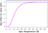	Fig. D.1 OTP ratio of H₂S as a function of spin temperature (Eq. (D.1)).
In the text

Current usage metrics show cumulative count of Article Views (full-text article views including HTML views, PDF and ePub downloads, according to the available data) and Abstracts Views on Vision4Press platform.

Data correspond to usage on the plateform after 2015. The current usage metrics is available 48-96 hours after online publication and is updated daily on week days.

Initial download of the metrics may take a while.

[1] Aguado, A., & Paniagua, M. 1992, J. Chem. Phys., 96, 1265 [NASA ADS] [CrossRef] [Google Scholar]

[2] Aguado, A., Tablero, C., & Paniagua, M. 2001, Comput. Phys. Comm., 134, 97 [NASA ADS] [CrossRef] [Google Scholar]

[3] Aguado, A., Barragan, P., Prosmiti, R., et al. 2010, J. Chem. Phys., 133, 024306 [NASA ADS] [CrossRef] [Google Scholar]

[4] Agúndez, M., & Wakelam, V. 2013, Chemical Reviews, 113, 8710 [Google Scholar]

[5] Agúndez, M., Goicoechea, J. R., Cernicharo, J., Faure, A., & Roueff, E. 2010, ApJ, 713, 662 [NASA ADS] [CrossRef] [Google Scholar]

[6] Allers, K. N., Jaffe, D. T., Lacy, J. H., Draine, B. T., & Richter, M. J. 2005, ApJ, 630, 368 [NASA ADS] [CrossRef] [Google Scholar]

[7] Anders, E., & Grevesse, N. 1989, Geochim. Cosmochim. Acta, 53, 197 [Google Scholar]

[8] Andree-Labsch, S., Ossenkopf-Okada, V., & Röllig, M. 2017, A&A, 598, A2 [NASA ADS] [CrossRef] [EDP Sciences] [Google Scholar]

[9] Anicich, V. G. 2003, An Index Of The Literature For Bimolecular Gas Phase Cation-Molecule Reaction Kinetics (California: JPL Publication), 1 [Google Scholar]

[10] Arab, H., Abergel, A., Habart, E., et al. 2012, A&A, 541, A19 [NASA ADS] [CrossRef] [EDP Sciences] [Google Scholar]

[11] Asplund, M., Grevesse, N., Sauval, A. J., & Scott, P. 2009, ARA&A, 47, 481 [NASA ADS] [CrossRef] [Google Scholar]

[12] Azzam, A. A. A., Yurchenko, S. N., Tennyson, J., Martin-Drumel, M.-A., & Pirali, O. 2013, J. Quant. Spectr. Rad. Transf., 130, 341 [NASA ADS] [CrossRef] [Google Scholar]

[13] Badnell, N. R. 1991, ApJ, 379, 356 [NASA ADS] [CrossRef] [Google Scholar]

[14] Bally, J. 2008, Overview of the Orion Complex, ed. B. Reipurth (USA: Nasa), 459 [Google Scholar]

[15] Bañares, L., Aoiz, F. J., Honvault, P., Bussery-Honvault, B., & Launay, J.-M. 2003, J. Chem. Phys., 118, 565 [Google Scholar]

[16] Bañares, L., Aoiz, F. J., Honvault, P., & Launay, J.-M. 2004, J. Phys. Chem., 108, 1616 [Google Scholar]

[17] Black, J. H. 1998, Faraday Discuss., 109, 257 [NASA ADS] [CrossRef] [Google Scholar]

[18] Bonnet, L., & Rayez, J.-C. 1997, Chem. Phys. Lett., 277, 183 [NASA ADS] [CrossRef] [Google Scholar]

[19] Bonnet, L., & Rayez, J.-C. 2004, Chem. Phys. Lett., 397, 106 [NASA ADS] [CrossRef] [Google Scholar]

[20] Brittain, A., Coolbroth, K., & Boogert, A. 2020, AAS Meeting Abstracts, 236, 247.08 [NASA ADS] [Google Scholar]

[21] Bron, E., Le Bourlot, J., & Le Petit, F. 2014, A&A, 569, A100 [NASA ADS] [CrossRef] [EDP Sciences] [Google Scholar]

[22] Bron, E., Agúndez, M., Goicoechea, J. R., & Cernicharo, J. 2018, ArXiv eprints [arXiv:1801.01547] [Google Scholar]

[23] Buckinghan, A. D. 1967, Adv. Chem. Phys., 12, 107 [CrossRef] [Google Scholar]

[24] Burton, M. G., Hollenbach, D. J., & Tielens, A. G. G. M. 1990, ApJ, 365, 620 [NASA ADS] [CrossRef] [Google Scholar]

[25] Calmonte, U., Altwegg, K., Balsiger, H., et al. 2016, MNRAS, 462, S253 [CrossRef] [Google Scholar]

[26] Cardelli, J. A., Clayton, G. C., & Mathis, J. S. 1989, ApJ, 345, 245 [NASA ADS] [CrossRef] [Google Scholar]

[27] Caselli, P., Keto, E., Pagani, L., et al. 2010, A&A, 521, L29 [NASA ADS] [CrossRef] [EDP Sciences] [Google Scholar]

[28] Caselli, P., Keto, E., Bergin, E. A., et al. 2012, ApJ, 759, L37 [Google Scholar]

[29] Charnley, S. B. 1997, ApJ, 481, 396 [NASA ADS] [CrossRef] [Google Scholar]

[30] Choi, Y., van der Tak, F. F. S., Bergin, E. A., & Plume, R. 2014, A&A, 572, L10 [Google Scholar]

[31] Collings, M. P., Anderson, M. A., Chen, R., et al. 2004, MNRAS, 354, 1133 [NASA ADS] [CrossRef] [Google Scholar]

[32] Crockett, N. R., Bergin, E. A., Neill, J. L., et al. 2014, ApJ, 781, 114 [NASA ADS] [CrossRef] [Google Scholar]

[33] Cruz-Diaz, G. A., Muñoz Caro, G. M., Chen, Y. J., & Yih, T. S. 2014, A&A, 562, A119 [NASA ADS] [CrossRef] [EDP Sciences] [Google Scholar]

[34] Cuadrado, S., Goicoechea, J. R., Pilleri, P., et al. 2015, A&A, 575, A82 [NASA ADS] [CrossRef] [EDP Sciences] [Google Scholar]

[35] Cuadrado, S., Goicoechea, J. R., Roncero, O., et al. 2016, A&A, 596, L1 [NASA ADS] [CrossRef] [EDP Sciences] [Google Scholar]

[36] Cuadrado, S., Goicoechea, J. R., Cernicharo, J., et al. 2017, A&A, 603, A124 [NASA ADS] [CrossRef] [EDP Sciences] [Google Scholar]

[37] Cuadrado, S., Salas, P., Goicoechea, J. R., et al. 2019, A&A, 625, L3 [CrossRef] [EDP Sciences] [Google Scholar]

[38] Dagdigian, P. J. 2019a, MNRAS, 487, 3427 [CrossRef] [Google Scholar]

[39] Dagdigian, P. J. 2019b, J. Chem. Phys., 150, 084308 [CrossRef] [Google Scholar]

[40] Dagdigian, P. J. 2020, MNRAS, 494, 5239 [NASA ADS] [CrossRef] [Google Scholar]

[41] Dartois, E. 2005, Space Sci. Rev., 119, 293 [NASA ADS] [CrossRef] [Google Scholar]

[42] Davidson, E. R. 1975, J. Comp. Phys., 17, 87 [NASA ADS] [CrossRef] [MathSciNet] [Google Scholar]

[43] de Graauw, T., Helmich, F. P., Phillips, T. G., et al. 2010, A&A, 518, L6 [NASA ADS] [CrossRef] [EDP Sciences] [Google Scholar]

[44] Desrousseaux, B., Lique, F., Goicoechea, J. R., Quintas-Sánchez, E., & Dawes, R. 2021, A&A, 645, A8 [NASA ADS] [CrossRef] [EDP Sciences] [Google Scholar]

[45] Endres, C. P., Schlemmer, S., Schilke, P., Stutzki, J., & Müller, H. S. P. 2016, J. Mol. Spectr., 327, 95 [NASA ADS] [CrossRef] [Google Scholar]

[46] Esplugues, G. B., Viti, S., Goicoechea, J. R., & Cernicharo, J. 2014, A&A, 567, A95 [NASA ADS] [CrossRef] [EDP Sciences] [Google Scholar]

[47] Esplugues, G. B., Cazaux, S., Meijerink, R., Spaans, M., & Caselli, P. 2016, A&A, 591, A52 [NASA ADS] [CrossRef] [EDP Sciences] [Google Scholar]

[48] Farah, K., Muller-Plathe, F., & Bohm, M. C. 2012, Chem. Phys. Chem., 13, 1127 [Google Scholar]

[49] Faure, A., Halvick, P., Stoecklin, T., et al. 2017, MNRAS, 469, 612 [NASA ADS] [CrossRef] [Google Scholar]

[50] Freeman, A., & Williams, D. A. 1982, Ap&SS, 83, 417 [CrossRef] [Google Scholar]

[51] Fuente, A., Rodrıguez-Franco, A., Garcıa-Burillo, S., Martın-Pintado, J., & Black, J. H. 2003, A&A, 406, 899 [NASA ADS] [CrossRef] [EDP Sciences] [Google Scholar]

[52] Fuente, A., Cernicharo, J., Roueff, E., et al. 2016, A&A, 593, A94 [NASA ADS] [CrossRef] [EDP Sciences] [Google Scholar]

[53] Fuente, A., Goicoechea, J. R., Pety, J., et al. 2017, ApJ, 851, L49 [NASA ADS] [CrossRef] [Google Scholar]

[54] Fuente, A., Navarro, D. G., Caselli, P., et al. 2019, A&A, 624, A105 [NASA ADS] [CrossRef] [EDP Sciences] [Google Scholar]

[55] Garrod, R. T., Wakelam, V., & Herbst, E. 2007, A&A, 467, 1103 [NASA ADS] [CrossRef] [EDP Sciences] [Google Scholar]

[56] Genzel, R., & Stutzki, J. 1989, ARA&A, 27, 41 [NASA ADS] [CrossRef] [Google Scholar]

[57] Gerin, M., de Luca, M., Black, J., et al. 2010, A&A, 518, L110 [NASA ADS] [CrossRef] [EDP Sciences] [Google Scholar]

[58] Gerin, M., Neufeld, D. A., & Goicoechea, J. R. 2016, ARA&A, 54, 181 [NASA ADS] [CrossRef] [Google Scholar]

[59] Gibb, E. L., Whittet, D. C. B., Boogert, A. C. A., & Tielens, A. G. G. M. 2004, ApJS, 151, 35 [NASA ADS] [CrossRef] [PubMed] [Google Scholar]

[60] Godard, B., & Cernicharo, J. 2013, A&A, 550, A8 [NASA ADS] [CrossRef] [EDP Sciences] [Google Scholar]

[61] Godard, B., Falgarone, E., Gerin, M., et al. 2012, A&A, 540, A87 [NASA ADS] [CrossRef] [EDP Sciences] [Google Scholar]

[62] Godard, B., Falgarone, E., & Pineau des Forêts, G. 2014, A&A, 570, A27 [NASA ADS] [CrossRef] [EDP Sciences] [Google Scholar]

[63] Goicoechea, J. R., & Le Bourlot, J. 2007, A&A, 467, 1 [NASA ADS] [CrossRef] [EDP Sciences] [Google Scholar]

[64] Goicoechea, J. R., Pety, J., Gerin, M., et al. 2006, A&A, 456, 565 [NASA ADS] [CrossRef] [EDP Sciences] [Google Scholar]

[65] Goicoechea, J. R., Pety, J., Gerin, M., Hily-Blant, P., & Le Bourlot, J. 2009, A&A, 498, 771 [NASA ADS] [CrossRef] [EDP Sciences] [Google Scholar]

[66] Goicoechea, J. R., Joblin, C., Contursi, A., et al. 2011, A&A, 530, L16 [NASA ADS] [CrossRef] [EDP Sciences] [Google Scholar]

[67] Goicoechea, J. R., Cernicharo, J., Karska, A., et al. 2012, A&A, 548, A77 [NASA ADS] [CrossRef] [EDP Sciences] [Google Scholar]

[68] Goicoechea, J. R., Pety, J., Cuadrado, S., et al. 2016, Nature, 537, 207 [NASA ADS] [CrossRef] [Google Scholar]

[69] Goicoechea, J. R., Cuadrado, S., Pety, J., et al. 2017, A&A, 601, L9 [NASA ADS] [CrossRef] [EDP Sciences] [Google Scholar]

[70] Goicoechea, J. R., Santa-Maria, M. G., Bron, E., et al. 2019, A&A, 622, A91 [NASA ADS] [CrossRef] [EDP Sciences] [Google Scholar]

[71] Goicoechea, J. R., Pabst, C. H. M., Kabanovic, S., et al. 2020, A&A, 639, A1 [CrossRef] [EDP Sciences] [Google Scholar]

[72] Gómez-Carrasco, S., & Roncero, O. 2006, J. Chem. Phys., 125, 054102 [NASA ADS] [CrossRef] [PubMed] [Google Scholar]

[73] Graedel, T. E., Langer, W. D., & Frerking, M. A. 1982, ApJS, 48, 321 [NASA ADS] [CrossRef] [Google Scholar]

[74] Grozdanov, T. P., & Solov’ev, E. A. 1982, J. Phys. B, 15, 1195 [CrossRef] [Google Scholar]

[75] Guzmán, V. V., Goicoechea, J. R., Pety, J., et al. 2013, A&A, 560, A73 [NASA ADS] [CrossRef] [EDP Sciences] [Google Scholar]

[76] Habart, E., Dartois, E., Abergel, A., et al. 2010, A&A, 518, L116 [NASA ADS] [CrossRef] [EDP Sciences] [Google Scholar]

[77] Habing, H. J. 1968, Bull. Astron. Inst. Netherlands, 19, 421 [Google Scholar]

[78] Hama, T., Kouchi, A., & Watanabe, N. 2016, Science, 351, 65 [NASA ADS] [CrossRef] [Google Scholar]

[79] Hamilton, J. R., Faure, A., & Tennyson, J. 2018, MNRAS, 476, 2931 [NASA ADS] [CrossRef] [Google Scholar]

[80] Hasegawa, T. I., & Herbst, E. 1993, MNRAS, 261, 83 [NASA ADS] [CrossRef] [Google Scholar]

[81] Hatchell, J., Thompson, M. A., Millar, T. J., & MacDonald, G. H. 1998, A&A, 338, 713 [Google Scholar]

[82] He, J., Shi, J., Hopkins, T., Vidali, G., & Kaufman, M. J. 2015, ApJ, 801, 120 [NASA ADS] [CrossRef] [Google Scholar]

[83] Heays, A. N., Bosman, A. D., & van Dishoeck, E. F. 2017, A&A, 602, A105 [NASA ADS] [CrossRef] [EDP Sciences] [Google Scholar]

[84] Heikkilä, A., Johansson, L. E. B., & Olofsson, H. 1999, A&A, 344, 817 [NASA ADS] [Google Scholar]

[85] Herbst, E., DeFrees, D. J., & Koch, W. 1989, MNRAS, 237, 1057 [NASA ADS] [CrossRef] [Google Scholar]

[86] Herpin, F., Marseille, M., Wakelam, V., Bontemps, S., & Lis, D. C. 2009, A&A, 504, 853 [NASA ADS] [CrossRef] [EDP Sciences] [Google Scholar]

[87] Heyminck, S., Graf, U. U., Güsten, R., et al. 2012, A&A, 542, L1 [NASA ADS] [CrossRef] [EDP Sciences] [Google Scholar]

[88] Hogerheijde, M. R., Jansen, D. J., & van Dishoeck, E. F. 1995, A&A, 294, 792 [NASA ADS] [Google Scholar]

[89] Holdship, J., Jimenez-Serra, I., Viti, S., et al. 2019, ApJ, 878, 64 [NASA ADS] [CrossRef] [Google Scholar]

[90] Hollenbach, D. J., & Tielens, A. G. G. M. 1997, ARA&A, 35, 179 [NASA ADS] [CrossRef] [Google Scholar]

[91] Hollenbach, D., Kaufman, M. J., Bergin, E. A., & Melnick, G. J. 2009, ApJ, 690, 1497 [CrossRef] [Google Scholar]

[92] Hollenbach, D., Kaufman, M. J., Neufeld, D., Wolfire, M., & Goicoechea, J. R. 2012, ApJ, 754, 105 [NASA ADS] [CrossRef] [Google Scholar]

[93] Hosokawa, T., & Inutsuka, S.-i. 2006, ApJ, 646, 240 [NASA ADS] [CrossRef] [Google Scholar]

[94] Howk, J. C., Sembach, K. R., & Savage, B. D. 2006, ApJ, 637, 333 [NASA ADS] [CrossRef] [Google Scholar]

[95] Hrodmarsson, H. R., Garcia, G. A., Nahon, L., Loison, J.-C., & Gans, B. 2019, Physi. Chem. Chem. Phys., 21, 25907 [NASA ADS] [CrossRef] [Google Scholar]

[96] Indriolo, N., Neufeld, D. A., Gerin, M., et al. 2015, ApJ, 800, 40 [NASA ADS] [CrossRef] [Google Scholar]

[97] Ioppolo, S., Cuppen, H. M., Romanzin, C., van Dishoeck, E. F., & Linnartz, H. 2008, ApJ, 686, 1474 [NASA ADS] [CrossRef] [Google Scholar]

[98] Jansen, D. J., Spaans, M., Hogerheijde, M. R., & van Dishoeck, E. F. 1995, A&A, 303, 541 [NASA ADS] [Google Scholar]

[99] Jiménez-Escobar, A., & Muñoz Caro, G. M. 2011, A&A, 536, A91 [NASA ADS] [CrossRef] [EDP Sciences] [Google Scholar]

[100] Jiménez-Serra, I., Zhang, Q., Viti, S., Martín-Pintado, J., & de Wit, W. J. 2012, ApJ, 753, 34 [NASA ADS] [CrossRef] [Google Scholar]

[101] Joblin, C., Bron, E., Pinto, C., et al. 2018, A&A, 615, A129 [NASA ADS] [CrossRef] [EDP Sciences] [Google Scholar]

[102] Johnson, B. R. 1987, J. Chem. Phys., 86, 1445 [NASA ADS] [CrossRef] [Google Scholar]

[103] Kaplan, K. F., Dinerstein, H. L., Oh, H., et al. 2017, ApJ, 838, 152 [NASA ADS] [CrossRef] [Google Scholar]

[104] Karplus, M., Porter, R. N., & Sharma, R. D. 1965, J. Chem. Phys., 43, 3259 [NASA ADS] [CrossRef] [Google Scholar]

[105] Kirsanova, M. S., & Wiebe, D. S. 2019, MNRAS, 486, 2525 [CrossRef] [Google Scholar]

[106] Klisch, E., Klaus, T., Belov, S. P., et al. 1996, ApJ, 473, 1118 [NASA ADS] [CrossRef] [Google Scholar]

[107] Kłos, J., Lique, F., & Alexander, M. H. 2009, Chem. Phys. Lett., 476, 135 [NASA ADS] [CrossRef] [Google Scholar]

[108] Knizia, G., Adler, T. B., & Werner, H. J. 2009, J. Chem. Phys., 130, 054104 [NASA ADS] [CrossRef] [Google Scholar]

[109] Laas, J. C., & Caselli, P. 2019, A&A, 624, A108 [CrossRef] [EDP Sciences] [Google Scholar]

[110] Le Bourlot, J., Le Petit, F., Pinto, C., Roueff, E., & Roy, F. 2012, A&A, 541, A76 [NASA ADS] [CrossRef] [EDP Sciences] [Google Scholar]

[111] Lee, T. A. 1968, ApJ, 152, 913 [NASA ADS] [CrossRef] [Google Scholar]

[112] Le Petit, F., Nehmé, C., Le Bourlot, J., & Roueff, E. 2006, ApJS, 164, 506 [NASA ADS] [CrossRef] [EDP Sciences] [Google Scholar]

[113] Leurini, S., Rolffs, R., Thorwirth, S., et al. 2006, A&A, 454, L47 [NASA ADS] [CrossRef] [EDP Sciences] [Google Scholar]

[114] Levine, R. D., & Bernstein, R. B. 1987, Mol Reaction Dynamics and Chemical Reactivity (Oxford: Oxford University Press) [Google Scholar]

[115] Lique, F., Zanchet, A., Bulut, N., Goicoechea, J. R., & Roncero, O. 2020, A&A, 638, A72 [NASA ADS] [CrossRef] [EDP Sciences] [Google Scholar]

[116] Lis, D. C., Bergin, E. A., Schilke, P., & van Dishoeck, E. F. 2013, J. Phys. Chem. A, 117, 9661 [CrossRef] [Google Scholar]

[117] Lucas, R., & Liszt, H. S. 2002, A&A, 384, 1054 [NASA ADS] [CrossRef] [EDP Sciences] [Google Scholar]

[118] Maiti, B., Schatz, G. C., & Lendvay, G. 2004, J. Phys. Chem. A, 108, 8772 [NASA ADS] [CrossRef] [Google Scholar]

[119] Marconi, A., Testi, L., Natta, A., & Walmsley, C. M. 1998, A&A, 330, 696 [NASA ADS] [Google Scholar]

[120] Martín, S., Mauersberger, R., Martín-Pintado, J., Henkel, C., & García-Burillo, S. 2006, ApJS, 164, 450 [NASA ADS] [CrossRef] [Google Scholar]

[121] Martín, S., Krips, M., Martín-Pintado, J., et al. 2011, A&A, 527, A36 [NASA ADS] [CrossRef] [EDP Sciences] [Google Scholar]

[122] Martin-Drumel, M. A., Eliet, S., Pirali, O., et al. 2012, Chem. Phys. Lett., 550, 8 [CrossRef] [Google Scholar]

[123] Melnick, G. J., Tolls, V., Goldsmith, P. F., et al. 2012, ApJ, 752, 26 [NASA ADS] [CrossRef] [Google Scholar]

[124] Melnick, G. J., Tolls, V., Snell, R. L., et al. 2020, ApJ, 892, 22 [CrossRef] [Google Scholar]

[125] Menten, K. M., Wyrowski, F., Belloche, A., et al. 2011, A&A, 525, A77 [NASA ADS] [CrossRef] [EDP Sciences] [Google Scholar]

[126] Millar, T. J., & Herbst, E. 1990, A&A, 231, 466 [NASA ADS] [Google Scholar]

[127] Millar, T. J., Adams, N. G., Smith, D., Lindinger, W., & Villinger, H. 1986, MNRAS, 221, 673 [NASA ADS] [CrossRef] [Google Scholar]

[128] Minissale, M., & Dulieu, F. 2014, J. Chem. Phys., 141, 014304 [NASA ADS] [CrossRef] [Google Scholar]

[129] Minissale, M., Dulieu, F., Cazaux, S., & Hocuk, S. 2016, A&A, 585, A24 [NASA ADS] [CrossRef] [EDP Sciences] [Google Scholar]

[130] Mumma, M. J., Weaver, H. A., & Larson, H. P. 1987, A&A, 187, 419 [NASA ADS] [Google Scholar]

[131] Nagy, T., & Lendvay, G. 2017, J. Phys. Chem. Lett., 8, 4621 [CrossRef] [Google Scholar]

[132] Nagy, Z., Van der Tak, F. F. S., Ossenkopf, V., et al. 2013, A&A, 550, A96 [NASA ADS] [CrossRef] [EDP Sciences] [Google Scholar]

[133] Nagy, Z., Choi, Y., Ossenkopf-Okada, V., et al. 2017, A&A, 599, A22 [NASA ADS] [CrossRef] [EDP Sciences] [Google Scholar]

[134] Navarro-Almaida, D., Le Gal, R., Fuente, A., et al. 2020, A&A, 637, A39 [CrossRef] [EDP Sciences] [Google Scholar]

[135] Neufeld, D. A., Nisini, B., Giannini, T., et al. 2009, ApJ, 706, 170 [NASA ADS] [CrossRef] [Google Scholar]

[136] Neufeld, D. A., Goicoechea, J. R., Sonnentrucker, P., et al. 2010, A&A, 521, L10 [NASA ADS] [CrossRef] [EDP Sciences] [Google Scholar]

[137] Neufeld, D. A., Falgarone, E., Gerin, M., et al. 2012, A&A, 542, L6 [NASA ADS] [CrossRef] [EDP Sciences] [Google Scholar]

[138] Neufeld, D. A., Godard, B., Gerin, M., et al. 2015, A&A, 577, A49 [NASA ADS] [CrossRef] [EDP Sciences] [Google Scholar]

[139] Oba, Y., Tomaru, T., Lamberts, T., Kouchi, A., & Watanabe, N. 2018, Nat. Astron., 2, 228 [NASA ADS] [CrossRef] [Google Scholar]

[140] O’Dell, C. R. 2001, ARA&A, 39, 99 [NASA ADS] [CrossRef] [Google Scholar]

[141] Pabst, C., Higgins, R., Goicoechea, J. R., et al. 2019, Nature, 565, 618 [NASA ADS] [CrossRef] [Google Scholar]

[142] Pabst, C. H. M., Goicoechea, J. R., Teyssier, D., et al. 2020, A&A, 639, A2 [CrossRef] [EDP Sciences] [Google Scholar]

[143] Palumbo, M. E., Geballe, T. R., & Tielens, A. G. G. M. 1997, ApJ, 479, 839 [NASA ADS] [CrossRef] [Google Scholar]

[144] Pankonin, V., & Walmsley, C. M. 1978, A&A, 64, 333 [NASA ADS] [Google Scholar]

[145] Parikka, A., Habart, E., Bernard-Salas, J., et al. 2017, A&A, 599, A20 [NASA ADS] [CrossRef] [EDP Sciences] [Google Scholar]

[146] Pellegrini, E. W., Baldwin, J. A., Ferland, G. J., Shaw, G., & Heathcote, S. 2009, ApJ, 693, 285 [NASA ADS] [CrossRef] [Google Scholar]

[147] Peterson, K. A., Adler, T. B., & Werner, H. J. 2008, J. Chem. Phys., 128, 084102 [NASA ADS] [CrossRef] [Google Scholar]

[148] Pineau des Forets, G., Flower, D. R., Hartquist, T. W., & Dalgarno, A. 1986, MNRAS, 220, 801 [NASA ADS] [CrossRef] [Google Scholar]

[149] Prasad, S. S., & Huntress, W. T., J. 1980, ApJS, 43, 1 [NASA ADS] [CrossRef] [Google Scholar]

[150] Prasad, S. S., & Huntress, W. T., J. 1982, ApJ, 260, 590 [NASA ADS] [CrossRef] [Google Scholar]

[151] Putaud, T., Michaut, X., Le Petit, F., Roueff, E., & Lis, D. C. 2019, A&A, 632, A8 [NASA ADS] [CrossRef] [EDP Sciences] [Google Scholar]

[152] Qu, C., & Bowman, J. M. 2016, J. Phys. Chem. A, 120, 4988 [CrossRef] [Google Scholar]

[153] Rivière-Marichalar, P., Fuente, A., Goicoechea, J. R., et al. 2019, A&A, 628, A16 [NASA ADS] [CrossRef] [EDP Sciences] [Google Scholar]

[154] Roelfsema, P. R., Helmich, F. P., Teyssier, D., et al. 2012, A&A, 537, A17 [NASA ADS] [CrossRef] [EDP Sciences] [Google Scholar]

[155] Roncero, O., Zanchet, A., & Aguado, A. 2018, Phys. Chem. Chem. Phys., 20, 25951 [NASA ADS] [CrossRef] [Google Scholar]

[156] Rosenthal, D., Bertoldi, F., & Drapatz, S. 2000, A&A, 356, 705 [NASA ADS] [Google Scholar]

[157] Sandford, S. A., & Allamandola, L. J. 1988, Icarus, 76, 201 [NASA ADS] [CrossRef] [Google Scholar]

[158] Sanz-Sanz, C., Roncero, O., Paniagua, M., & Aguado, A. 2013, J. Chem. Phys., 139, 184302 [NASA ADS] [CrossRef] [Google Scholar]

[159] Shiozaki, T., & Werner, H.-J. 2013, Mol. Phys., 111, 607 [NASA ADS] [CrossRef] [Google Scholar]

[160] Smirnov, G. T., Sorochenko, R. L., & Walmsley, C. M. 1995, A&A, 300, 923 [NASA ADS] [Google Scholar]

[161] Smith, R. G. 1991, MNRAS, 249, 172 [NASA ADS] [CrossRef] [Google Scholar]

[162] Sofia, U. J., Lauroesch, J. T., Meyer, D. M., & Cartledge, S. I. B. 2004, ApJ, 605, 272 [NASA ADS] [CrossRef] [Google Scholar]

[163] Stecher, T. P., & Williams, D. A. 1972, ApJ, 177, L141 [NASA ADS] [CrossRef] [Google Scholar]

[164] Sternberg, A., & Dalgarno, A. 1995, ApJS, 99, 565 [NASA ADS] [CrossRef] [Google Scholar]

[165] Stoerzer, H., Stutzki, J., & Sternberg, A. 1995, A&A, 296, L9 [NASA ADS] [Google Scholar]

[166] Stowe, G. F., Schultz, R. H., Wright, C. A., & Armentrout, P. B. 1990, Int. J. Mass Spectr. Ion Proc., 100, 377 [Google Scholar]

[167] Tablero, C., Aguado, A., & Paniagua, M. 2001, Comput. Phys. Comm., 140, 412 [NASA ADS] [CrossRef] [Google Scholar]

[168] Taquet, V., Furuya, K., Walsh, C., & van Dishoeck, E. F. 2016, MNRAS, 462, S99 [Google Scholar]

[169] Tercero, B., Cernicharo, J., Pardo, J. R., & Goicoechea, J. R. 2010, A&A, 517, A96 [NASA ADS] [CrossRef] [EDP Sciences] [Google Scholar]

[170] Tieftrunk, A., Pineau des Forets, G., Schilke, P., & Walmsley, C. M. 1994, A&A, 289, 579 [Google Scholar]

[171] Tielens, A. G. G. M. 2010, The Physics and Chemistry of the Interstellar Medium (Cambridge: Cambridge University Press) [Google Scholar]

[172] Tielens, A. G. G. M., & Hagen, W. 1982, A&A, 114, 245 [Google Scholar]

[173] Tielens, A. G. G. M., & Hollenbach, D. 1985, ApJ, 291, 722 [Google Scholar]

[174] Tielens, A. G. G. M., Meixner, M. M., van der Werf, P. P., et al. 1993, Science, 262, 86 [NASA ADS] [CrossRef] [PubMed] [Google Scholar]

[175] Turner, B. E. 1996, ApJ, 468, 694 [NASA ADS] [CrossRef] [Google Scholar]

[176] van der Tak, F. F. S., Boonman, A. M. S., Braakman, R., & van Dishoeck, E. F. 2003, A&A, 412, 133 [NASA ADS] [CrossRef] [EDP Sciences] [Google Scholar]

[177] van der Tak, F. F. S., Black, J. H., Schöier, F. L., Jansen, D. J., & van Dishoeck, E. F. 2007, A&A, 468, 627 [NASA ADS] [CrossRef] [EDP Sciences] [Google Scholar]

[178] van der Tak, F. F. S., Nagy, Z., Ossenkopf, V., et al. 2013, A&A, 560, A95 [NASA ADS] [CrossRef] [EDP Sciences] [Google Scholar]

[179] van der Werf, P. P., Stutzki, J., Sternberg, A., & Krabbe, A. 1996, A&A, 313, 633 [NASA ADS] [Google Scholar]

[180] van der Werf, P. P., Goss, W. M., & O’Dell, C. R. 2013, ApJ, 762, 101 [NASA ADS] [CrossRef] [Google Scholar]

[181] van der Wiel, M. H. D., van der Tak, F. F. S., Ossenkopf, V., et al. 2009, A&A, 498, 161 [NASA ADS] [CrossRef] [EDP Sciences] [Google Scholar]

[182] van Dishoeck, E. F. 2004, ARA&A, 42, 119 [NASA ADS] [CrossRef] [Google Scholar]

[183] Velilla, L., Lepetit, B., Aguado, A., Beswick, J., & Paniagua, M. 2008, J. Chem. Phys., 129, 084307 [CrossRef] [PubMed] [Google Scholar]

[184] Vidal, T. H. G., Loison, J.-C., Jaziri, A. Y., et al. 2017, MNRAS, 469, 435 [Google Scholar]

[185] Wakelam, V., Loison, J. C., Mereau, R., & Ruaud, M. 2017, Mol. Astrophys., 6, 22 [NASA ADS] [CrossRef] [EDP Sciences] [Google Scholar]

[186] Walmsley, C. M., Natta, A., Oliva, E., & Testi, L. 2000, A&A, 364, 301 [NASA ADS] [Google Scholar]

[187] Werner, H. J., & Knowles, P. J. 1988a, J. Chem. Phys., 89, 5803 [NASA ADS] [CrossRef] [Google Scholar]

[188] Werner, H. J., & Knowles, P. J. 1988b, Chem. Phys. Lett., 145, 514 [NASA ADS] [CrossRef] [Google Scholar]

[189] Werner, H.-J., Knowles, P. J., Knizia, G., Manby, F. R., & Schütz, M. 2012, WIREs Comput. Mol. Sci., 2, 242 [CrossRef] [Google Scholar]

[190] Wyrowski, F., Schilke, P., Hofner, P., & Walmsley, C. M. 1997, ApJ, 487, L171 [NASA ADS] [CrossRef] [Google Scholar]

[191] Yamamura, I., Kawaguchi, K., & Ridgway, S. T. 2000, ApJ, 528, L33 [NASA ADS] [CrossRef] [Google Scholar]

[192] Young, E. T., Becklin, E. E., Marcum, P. M., et al. 2012, ApJ, 749, L17 [NASA ADS] [CrossRef] [Google Scholar]

[193] Zanchet, A., Roncero, O., González-Lezana, T., et al. 2009, J. Phys. Chem. A, 113, 14488 [CrossRef] [PubMed] [Google Scholar]

[194] Zanchet, A., Agúndez, M., Herrero, V. J., Aguado, A., & Roncero, O. 2013a, AJ, 146, 125 [NASA ADS] [CrossRef] [Google Scholar]