| Issue |
A&A
Volume 647, March 2021
|
|
|---|---|---|
| Article Number | A175 | |
| Number of page(s) | 19 | |
| Section | Planets and planetary systems | |
| DOI | https://doi.org/10.1051/0004-6361/202039706 | |
| Published online | 29 March 2021 | |
How planets grow by pebble accretion
III. Emergence of an interior composition gradient★
1
Department of Astronomy, Tsinghua University,
Beijing
100084,
PR China
e-mail: This email address is being protected from spambots. You need JavaScript enabled to view it.
2
Department of Natural Sciences, The Open University of Israel,
Ra’anana
43537,
Israel
3
Astrophysics Research Center of the Open University (ARCO), The Open University of Israel,
Ra’anana
43537,
Israel
4
Institute of Astronomy, University of Cambridge,
Madingley Road,
Cambridge
CB3 0HA,
USA
Received:
18
October
2020
Accepted:
3
February
2021
Abstract
During their formation, planets form large, hot atmospheres due to the ongoing accretion of solids. It has been customary to assume that all solids end up at the center, constituting a “core” of refractory materials, whereas the envelope remains metal-free. However, recent work, as well as observations by the Juno mission, indicate that the distinction may not be so clear cut. Indeed, small silicate, pebble-sized particles will sublimate in the atmosphere when they hit the sublimation temperature (T ~ 2000 K). In this paper we extend previous analytical work to compute the properties of planets within such a pebble accretion scenario. We conduct 1D numerical calculations of the atmosphere of an accreting planet, solving the stellar structure equations, augmented by a nonideal equation of state that describes a hydrogen and helium-silicate vapor mixture. Calculations terminate at the point where the total mass in metal is equal to that of the H+He gas, which we numerically confirm as the onset of runaway gas accretion. When pebbles sublimate before reaching the core, insufficient (accretion) energy is available to mix dense, vapor-rich lower layers with the higher layers of lower metallicity. A gradual structure in which Z decreases with radius is therefore a natural outcome of planet formation by pebble accretion. We highlight, furthermore, that (small) pebbles can act as the dominant source of opacity, preventing rapid cooling and presenting a channel for (mini-)Neptunes to survive in gas-rich disks. Nevertheless, once pebble accretion subsides, the atmosphere rapidly clears followed by runaway gas accretion. We consider atmospheric recycling to be the most probable mechanism to have stalled the growth of the envelopes of these planets.
Key words: planets and satellites: formation / planets and satellites: composition / planets and satellites: physical evolution / planet-disk interactions / methods: numerical
Movie associated to Fig. 5 is available at https://www.aanda.org
© ESO 2021
1 Introduction
The core accretion paradigm considers planet formation to be a two-staged process: first a “solid" core forms by accreting refractory material, and subsequently, when the core has become sufficiently massive, metal-poor gas pours in to form the envelope of a (giant) planet (Pollack et al. 1996; Hubickyj et al. 2005; Mordasini et al. 2012). However, the assumption of a sharp division between metal-rich assembly for the core and metal-poor assembly for the gaseous envelope is problematic, as these two components form together. A planet first begins to bind a small proto-atmosphere when the planet’s Bondi radius exceeds the core radius, corresponding to a mass of ~ 0.1 M⊕ which is dependent on disk location. The atmosphere grows into a larger envelope as the planet gains mass. In the classical scenario, the composition of this envelope is presumed to remain the same as that of the nebular gas. This assumption is now increasingly being questioned, as the accreting solids may end up enriching the atmosphere (to some extent) before they reach the core. Stevenson (1982) already highlighted the importance of atmosphere enrichment. By increasing the molecular weight, the scale height of the atmosphere is decreased, allowing the envelope to contract and to become more massive. More recently, Hori & Ikoma (2011) and Venturini et al. (2015, 2016) argued that envelope enrichment by H2O would greatly reduce the critical core mass, that is, the mass where gas accretion accelerates.
As the amount of envelope enrichment is crucial to the thermodynamical evolution of the planet, the question arises as to the fate of the solids as they traverse through the envelope toward the core. In the classical model, any impactors that enter the envelope are assumed to remain intact until they reach the core, where they add their mass and liberate their gravitational energy. This requires that impactors be strong enough to overcome disruption due to the dynamical pressure they experience in their descent through the envelope and large enough to avoid thermal ablation. In practice, this requires impactors to be rigid (rubble piles will disrupt) and to exceed ~10 km, with this size threshold increasing with planet mass (Podolak et al. 1988; Mordasini et al. 2015; Pinhas et al. 2016; Brouwers et al. 2018; Valletta & Helled 2019; Brouwers & Ormel 2020). The assumption that solids reach the core therefore becomes especially questionable when they are small.
In the last decade, pebble accretion has emerged as a new contender to make large cores (Ormel & Klahr 2010; Lambrechts & Johansen 2012; Bitsch et al. 2015; Johansen & Lambrechts 2017). Pebbles, by virtue of their small size, settle gently towards the core. Therefore, it can be assumed that they are in thermal equilibrium with the gas; that is, their sublimation is regulated by the saturation vapor pressure of the material. They will evaporate entirely when the ambient temperature exceeds the condensation temperature, which is around ~300 K for H2 O or ~2000 K for silicates.
In Brouwers et al. (2018, henceforth Paper I) we numerically calculated the point where silicate impactors fully evaporate in the atmosphere and where direct core growth terminates. Importantly, we relaxed the assumption that enrichment is uniform in the envelope. Instead, the saturation vapor pressure limits the atmosphere intake of pollutants, which renders the enrichment strongly inhomogeneous. The outer layers are barely affected and remain dominated by H+He (hydrogen and helium), whereas the hot regions close to the core first become dominant in vapor. Of course, the nature of the enrichment depends on the materials from which the accreted solids are composed (rock vs. volatile). In this work, we focus on silicate-rich impactors. With increasing mass, the envelope becomes hotter and is capable of absorbing an increasing amount of vapor, until solids no longer reach the core, marking the end of the direct growth phase (Phase I).
With an analytical model, Brouwers & Ormel (2020, henceforth Paper II) described the subsequent evolution of such vapor-rich planets. In Phase II, growth is dominated by the envelope, which vaporizes and absorbs all incoming solid material. At the same time, H+He nebular gas is accreted and Paper II provides an expression for the critical metal mass, which is the mass where the total amount of metal (core+vapor) is equal to the mass in H+He. However, in the case of (sub)Neptunes and lower mass planets, the envelopenever reaches this point. Accretion of pebbles may shut off at some point, in which case the envelope evolves through Kelvin-Helmholtz contraction (Phase III). Finally, after the planet has emerged from the natal disk and has cooled for ~1 Gyr (Phase IV), conditions may again become suitable for supersaturation and a renewed phase of core growth.
While the (semi-)analytical modelling provides a useful roadmap, models necessarily include assumptions to make them mathematically tractable. Specifically, we employed the ideal equation of state and (for Paper II) made the assumption that all vapor is confined in an inner homogeneous layer, which is convective. The caveat to the first assumption is that the rather compressible ideal gas results in very high vapor densities, while the assumption of a convective interior implies the presence of energy to mix the vapor with the H+He gas. Numerical calculations are necessary to re-examine the conclusions reached in our previous works.
To this end, we employ a nonideal, tabulated equation of state (EoS) for the H+He (Saumon et al. 1995), and for the SiO2 vapor (Faik et al. 2018). We calculate the EoS of the three-component mixture self-consistently at each location in time following Vazan et al. (2013). Our numerical model switches to a wet adiabat in regions where the vapor is saturated. In particular, we relax the assumption that the interior is entirely convective or conductive. Instead, we condition convective transport and mixing with the appearance of positive luminosity, because mixing stratified SiO2 vapor consumes energy.
We then apply this model to understand the origin of close-in super-Earth and mini-Neptune planets, which our galaxy harbors in great numbers (Fressin et al. 2013; Petigura et al. 2013; Zhu et al. 2018), from a pebble accretion perspective. From arguments based on evaporation, the consensus is that these planets were born early, in the gas-rich phase, made out of terrestrial materials with a thick H+He atmosphere (Wu & Lithwick 2013; Lopez & Fortney 2014; Fulton et al. 2017; Owen & Wu 2017). This could simply reflect a compact and dense progenitor disk (Chiang & Laughlin 2013), or indicate large-scale transport of either the planets themselves or of the planet building blocks (Hansen 2009). The case for pebble accretion is attractive, as the pebble flux can be maintained over a long time (Lambrechts et al. 2014, 2019) and, unlike with planet migration, a rocky composition can be expected as the H2 O vapor will sublimate off pebbles when they cross the disk ice line. Furthermore, pebbles may contribute to the atmospheric opacity, which determines the thermal evolution of the planet (Ikoma et al. 2000; Hori & Ikoma 2010; Piso & Youdin 2014). We explore the possibility that pebbles regulate the envelope growth in this way.
A second application concerns the distribution of the vapor within the envelope. Recently, new insights have emerged from Jupiter’s gravitational moments measurement by the Juno mission. These infer that, instead of the classical pure-refractory core, the core is extended or “dilute” (Wahl et al. 2017; Debras & Chabrier 2019). The influence of the initial metallicity profile of the interiors of (giant) planets on its long-term evolution has now been well studied (Vazan et al. 2016, 2018; Lozovsky et al. 2017; Müller et al. 2020). Our previous works highlighted the potential for producing such dilute (vapor-rich) regions from formation. It is therefore time to outline what is predicted by the different planet-formation models for the internal structure of various types of planets, giants as well as (mini-)Neptunes (cf. Bodenheimer et al. 2018; Valletta & Helled 2020; Venturini & Helled 2020).
The plan of the paper is as follows. In Sect. 2 we outline the model. Our model solves the stellar structure equations using a boundary element solver. In Sect. 3 we present our results for about one hundred simulations where we vary a great number of parameters. We present profiles of temperature, density, and metallicity, and compare some of our results to the analytical predictions outlined in Paper II. In Sect. 4 we discuss the potential for pebble accretion to explain the formation of (mini-)Neptune planets and dilute cores. We list our conclusions in Sect. 5.
2 Model
Our model calculates the evolution of the core and envelope of an embedded, pebble-accreting planet. It includes elements from approaches applicable to planetesimal accretion (Stevenson 1982; Pollack et al. 1996; Rafikov 2006; Mordasini et al. 2012), as well as elements from studies that consider pure Kelvin-Helmholtz contraction (Ikoma et al. 2000; Piso & Youdin 2014; Coleman et al. 2017; Guilera et al. 2020). The envelope is assumed to be in hydrostatic equilibrium on dynamical timescales and in pressure equilibrium with the surrounding disk gas. This validates a quasi-steady approach. At each time, or snapshot, a steady solution to the stellar structure equations is found.
A key element of our approach is that we relax the standard assumption that accreting solids end up in the core. In Paper I we calculated the fraction of the incoming solids that end up in the envelope as silicate vapor, a number that steadily increases with time until all the accreted pebble flux is absorbed by the atmosphere. Here, we extend these calculations to the undersaturated state, which requires a model for the treatment of the silicate vapor.
2.1 Solidand vapor treatment
We consider a growing protoplanet embedded in a disk, accreting pebbles at a rate Ṁpeb. These pebbles partially or entirely vaporize in the envelope of the planet. Formally, the evolution of the vapor distribution is described by a (time-dependent) transport equation, accounting for mixing, deposition (through ablation), and rainout (e.g., Ormel & Min 2019). However, transport is usually ignored and the enrichment is taken to be uniform for simplicity. Nevertheless, in reality we can expect a stratified picture, reflecting the different condensation temperatures of volatile and refractory species (Iaroslavitz & Podolak 2007; Lozovsky et al. 2017). In the present work, we account for the inhomogeneous nature of enrichment, but consider a single refractory species (SiO2) for simplicity. We denote the density of the vaporized SiO2 as ρZ and that of the noncondensible H+He gas as ρxy. The metallicity of the gas is then Z = ρZ∕ρ = ρZ∕(ρZ + ρxy).
In Paper I, we covered the early phases of sublimation, where the vapor follows the saturation pressure, which is a strong function of temperature. Consequently, the vapor density profile is inhomogeneous. In the analytical model of Paper II weadded an inner layer below the saturated (cooler) region, where the temperature is hot enough for the vapor to be below saturation. In this layer (region 2a in Fig. 1), the vapor resides at uniform concentration, as it was assumed that the layer is convective. With time, the vapor concentration in this region Zcnv decreases with the accretion of nebular gas. However, the assumption that silicate vapor and nebular gas mix requires energy, which we found was not always available. This implies that the composition remains stratified to a certain degree. In order to incorporate the limitations of compositional mixing, we add a third region (2b) where the compositionis inhomogeneous in space but constant in time; the given mass shell is said to be “compositionally frozen” in time. The structure of the envelope is sketched in Fig. 1. In summary, the regions are:
- 1.
an outermost saturated region, where the composition follows the equilibrium metallicity
 (1)
(1) - 2a.
a well-mixed convective region of uniform composition with Z uniform and decreasing with time, Z = Zcnv(t),
- 2b.
a stratified, frozen region where the composition spatially varies, but where Z of a particular mass shell does not change with time, Z = Z(m).
Our model design regarding composition can be regarded as an improvement over a pure global treatment, where Z would be constant throughout the envelope. In our model, the composition is, respectively, quantified by the value of Z at previous times (region 2b), the constant Zcnv (region 2a), and Zsat, which is a function of temperature. The compositional gradient attains its steepest values in region 1, near the interface with region 2. Region 1 is by definition saturated. In saturated regions, the Ledoux (1947) convection criterion is not applicable, as the composition and temperature are no longer independent (e.g., Chambers 2017); the instability criterion is that of moist convection (Tremblin et al. 2019), which we include as a modified Schwarzschield criterion Sect. 2.4.3. Therefore, the model design choices avoid the explicit use of the Ledoux criterion.
The boundaries between these regions evolve with time and are set by the following conditions: Zcnv = Zsat for the boundary between regions 1 and 2a; and L > 0 globally for the boundary between regions 2a and 2b. (We note again that these regime boundaries only appear in Phase II, see below.) With time, both boundaries shift outward. The global condition for the luminosity requires an iterative approach – we increase riso until L becomes globally positive. Below, we review how these regions develop chronologically and how this is implemented in our code.
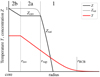 |
Fig. 1 Adopted model for the metallicity Z = ρZ∕ρ of the envelope. In region 1, the envelope is always saturated and the metallicity Z follows the saturation curve Zsat (gray), which is set by the saturation vapor pressure. Initially, when the entire envelope is saturated, only this region is present. Upon reaching Phase II a new region (2) develops that is undersaturated (Z < Zsat). In region 2a, convection ensures that the metallicity Zcnv is uniform. Region 2b represents a zone where convection does not operate due to lack of energy sources. Here, Z is constant in time for the same mass shell. With increasing accretion of H+He gas, Zcnv decreases and the region boundaries shift outwards. |
2.1.1 Phase I: direct core growth
In Phase I, only region 1 exists. During this time the planet’s envelope is sufficiently small and cold for refractories to survive thermal ablation and to make it to the core. However, the envelope absorbs as much vapor as it can – i.e., region 1 is saturated – and the amount of ablation increases with depth in the atmosphere, as the saturation vapor pressure is a strong function of temperature. This pressure can also be cast in terms of an equilibrium density  where vZ is the thermal velocity of SiO2. Hence, we assume in region 1 that ρZ = ρsat and define Zsat accordingly.
Initially, the amount of vapor absorbed by the envelope is small because T is low; most of the pebbles end up in the core. When the temperature approaches ~2000 K, sublimation becomes more significant and pebbles by virtue of their small size may evaporate entirely. Still, the fraction of vapor that the envelope can absorb is always limited to ρsat. In Paper I the impact trajectory of the pebbles and the vapor ablation rate were calculated explicitly. When it was found that ρz > ρsat, the excess vaporwas assumed to rain out to the core. In the present work we omit an impact model and simplify matters by assuming that solids always settle slowly enough for the atmosphere to become saturated at any point. This assumption is natural to pebbles. The duration of Phase I lasts until the point where the envelope has become hot enough to be subcritical (ρsat (T) > ρz); all silicate material dissolves and core growth terminates.
2.1.2 Phase II: envelope growth
The subsequent Phase II describes the phase where pebbles completely evaporate in the envelope. Core growth terminates and the envelope becomes undersaturated, meaning that Z < Zsat in the hotter regions (2a and 2b), while in the cooler outer region 1 Z = Zsat is maintained. The metallicity of the convective zone Zcnv, the solution for which is unknown (see Sect. 2.5), decreases with time. In Phase II this new parameter is substituted for the now known (fixed) core mass.
Phase II is also characterized by the development of the compositionally frozen region 2b. The boundary between regions 2a and 2b, r = riso, is another (unknown) parameter to the model. The condition we adopt is to demand that L ≥ 0 everywhere. If this is not satisfied, we let riso expand until L becomes positive. In general, the region within riso releases energy due to PdV compression, while mixing that takes place in region 2a consumes energy. The requirement that L > 0 for mixing (or rather that ∇rad ≫ 1 wherever L is positive in region 2a) may be replaced by a more stringent criterion amounting to L > Lmin. But this would simply amount to shifting the 2a–2b boundary.
Our choice for this rigid distinction between regions 2a and 2b warrants explanation. The more desired choice is for a local approach, for example, to freeze the composition wherever the luminosity becomes too small for convective transport. However, there are reasons, mainly computational in nature, that force us to choose differently. First, the local approach may result in many mutually isolated convective zones, each with different Zcnv. More problematic is that the numerical solver we have adopted simply cannot handle steep variations (let alone discontinuities) in the temperature gradient ∇, which arise when the luminosity becomes negative – the adiabatic index drops from a value consistent with convective transport (when L > 0), ∇ ≈0.2–0.5 to ≪ − 1 when L < 0. Thus, even though L may change gradually, ∇ will not. We therefore make the approximation that the structure is layered, characterized by one single “frozen” region. In reality, we find that within this region, the luminosity is generally positive, because the PdV -liberated heat from compression tends to outpace the increase in the internal energy. Still, this luminosity is insufficient to fully mix regions 2a and 2b. Presumably, in reality multiple small convective layers develop, each with a different composition(Rosenblum et al. 2011), but our numerical tool is not suited to implement such a multi-layer model effort.
The extent of the compositionally frozen zone is such that it (collectively) generates positive luminosity needed to mix the material above. For simplicity, the zone is modeled as isothermal. Keeping an adiabatic profile (apart from being inconsistent with the frozen assumption) requires large amounts of energy to support the high central temperatures. A negative ∇ for the frozen zone, on the other hand, implies that there is a net energy transport into the core. While this may partially develop because our core is of lower temperature, the ability of the core to transport energy in the direction of gravity (i.e., no convective transport) is questionable. Taking the region as a whole, the isothermal assumption can be justified as there are no obvious sources of energy (pebbles being deposited above this layer). Our situation therefore resembles the case in stellar evolution, where an isothermal stellar core develops after hydrogen burning moves away from the star’s core due to it being exhausted of hydrogen (Kippenhahn & Weigert 1990). Clearly, the assumption of ∇ = 0 across the entire regionis crude and a local treatment would be preferable. But in an averaged sense, it captures the general trend that a lack of energy sources causes ∇ to decrease.
2.1.3 Phase III: embedded cooling
In Phase III, pebble accretion terminates and gives way to pure Kelvin-Helmholtz contraction of the envelope. This phase is not associated with the introduction of a new region. We include Phase 3 simply by tapering off the pebble accretion rate:
![Mathematical equation: \begin{equation*} \dot{M}_{\mathrm{peb}} = \dot{M}_{\mathrm{peb,0}} \exp \left[ -A \left(\frac{t}{t_{\sigma}}\right)^n \right] ,\end{equation*}](/articles/aa/full_html/2021/03/aa39706-20/aa39706-20-eq3.png) (2)
(2)
where tσ = MZ,final∕Ṁpeb,0 is the timescale over which the pebble accretion rate subsides, MZ,final the final metal mass of the planet,  a constant to make ∫ Ṁpeb,0dt = MZ,final, and Γ(x) the Gamma function.
In most of our runs, we take an infinite and constant supply of pebbles MZ,final = tσ = ∞ for simplicity, but in runs where we do explore Phase III we choose MZ,final = 4, 6, and 8 M⊕ as representative for a mini-Neptune. We further choose n = 4 (A = 0.675) such that after t = tσ accretion of pebbles very rapidly subsides to zero.
2.1.4 Phase IV: isolated cooling
We define Phase IV as the phase where the protoplanetary disk dissipates, the outer layers of the atmosphere may evaporate, and where progressive cooling may cause the vapor to rain out. This phase is not considered in the present work, but is crucial to assess the viability of core-powered mass loss (Owen & Wu 2016; Gupta & Schlichting 2019; Paper II). As it covers the ~1 Gyr evolution, italso connects directly to the observed properties of exoplanets.
2.2 Envelope structure equations
We obtain the temperature (T) and pressure (P) profiles of the envelope by solving the stellar structure equations:
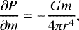 (3a)
(3a)
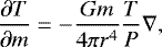 (3b)
(3b)
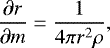 (3c)
(3c)
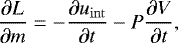 (3d)
(3d)
where ∇ = min(∇rad, ∇ad) (Schwarzschield criterion) with ∇rad the radiative gradient,
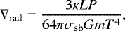 (4)
(4)
κ is the opacity, L the luminosity, σsb the Stefan-Boltzmann’s constant, and ∇ad the (wet) adiabatic gradient; see Sect. 2.4.3. Following Paper I, we use a simple power-law fit for the opacity, which we adopt from Lee & Chiang (2015):
 (5a)
(5a)
which is valid for our calculations at 0.2 au, and
 (5b)
(5b)
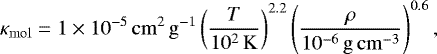
which is valid for 1 and 5 au. Expressions are fits to tables by Ferguson et al. (2005) and Freedman et al. (2014) and are evaluated at solar metallicity (Z = 0.02). Sublimation will raise Z but at this point envelopes have already become convective. As found by previous works, grains are not expected to survive for a long time in envelopes (Movshovitz et al. 2010; Mordasini 2014; Ormel 2014). Instead, we account for an opacity from pebbles:
 (6)
(6)
where Qeff is the efficiency coefficient (which evaluates to 2), speb the radius of thepebbles, and vsed is the sedimentation velocity. By assuming that gas drag and gravity balance, the sedimentation velocity of the pebble is vsed= Gmtstop∕r2. In Eq. (6) the first term is the opacity per unit mass dust, the second term the dust-to-gas ratio, and the stopping time tstop reads
![Mathematical equation: \begin{equation*} t_{\mathrm{stop}} = \frac{\rho_{\bullet} s_{\mathrm{peb}}}{v_{\mathrm{th}}\rho} \times \max \left[ 1, \frac{4s_{\mathrm{peb}}}{9l_{\mathrm{mfp}}} \right],\end{equation*}](/articles/aa/full_html/2021/03/aa39706-20/aa39706-20-eq13.png) (7)
(7)
where we account for the Epstein and Stokes drag law. We note that in Eq. (6) it is assumed that pebbles do not coagulate.
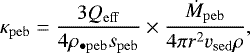
In addition to these equations, we integrate the metallicity Z in order to obtain the total amount of solids in the envelope:
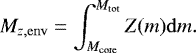 (8)
(8)
The total metal contents of the planets then changes as function of time
 (9)
(9)
which provides another boundary constraint.
In the above expressions, the gas density ρ, the internal energy uint, and the adiabatic index are obtained from an EoS (Sect. 2.4).
Model constants and boundary conditions.
2.3 Luminosity and core treatment
We considerthe energy conservation equation (Eq. (3d)) in integral form:
 (10)
(10)
where Ls are surface contributions (Piso & Youdin 2014). In preceding works (Mordasini et al. 2012; Piso & Youdin 2014; Venturini et al. 2016), energy conservation was applied at a specific radius (e.g., the radiative-convective boundary) and the corresponding L was assumed to be constant within this radius. In contrast, in the present work, Eq. (10) is used to find the luminosity at every mass shell, that is, L(m) becomes a local quantity. The energy E is then the total energy within shell m:
 (11)
(11)
where Φ(m) is the potential energy at mass level m, U(m) is the total internal energy interior to m, and Ecore is the energy of the core. The internal energy includes the latent heat of vaporization. The potential energy of the core is taken to be equal to that of a uniform sphere ( ), while its thermal energy (Ucore) follows from integration over the temperature structure within the core; that is,
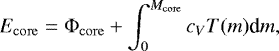 (12)
(12)
where the heat capacity is taken to be cV = 107 erg K-1 g-1 (Guillot et al. 1995; D’Angelo & Podolak 2015). It is assumed that no thermal transport takes place within the core. Hence, T(m) in Eq. (12) corresponds to the temperature at the bottom of the envelope at the time when pebbles became incorporated into the core. Indeed, pebbles, unlike planetesimals, adjust to the ambient temperature (Paper I). The core is for simplicity treated as thermally isolated, that is, further thermal evolution of the envelope will not affect it and vice versa. We also do not use an EoS for the core: it is instead characterized by a fixed density (Table 1).
2.4 Equation of state
We assume that hydrogen and helium are present at a mass ratio of X∕Y = 0.7∕0.3 = 2.33. In this work, we consider both the ideal EoS and a tabulated, nonideal EoS.
2.4.1 Ideal EoS
In the ideal EoS, the mean molecular weight μ of the gas mixture is
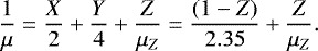 (13)
(13)
For SiO2, μZ = 60. Dissociation and ionization of SiO2 would reduce μ, but only in regions where Z ≈ 1.
Likewise, the heat capacity ratio of the gas is obtained by the weighted ratio of the individual heat capacities of hydrogen (H2), helium, and Z. We consider three translational degrees and two rotational degrees of freedom for the linear molecules H2 and SiO2. Because SiO2 becomes abundant at high temperatures, we also include its vibrational degrees (four). The total degrees of freedom for hydrogen, helium, and SiO2 are 5, 3, and 9, respectively. The weighted heat capacity is then
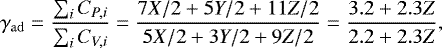 (14)
(14)
from which ∇ad = (γad − 1)∕γad follows.
The density and internal energy are:
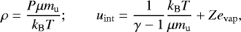 (15)
(15)
where evap is the latent heat of evaporation, which is the energy required to transform the solid pebbles to the gas phase. Hence, our γad ranges from 1.45 in the (outer) H- and He-dominated regions to γad = 1.22 in regions where metals dominate.
This ideal EoS is analytical and simplistic. Nonideal effects, such as ionization and dissociation, can in principle be included for hydrogen and helium (Ikoma et al. 2000; Lee et al. 2014), while still keeping an analytical approach. We refrain from considering these refinements in order to connect to our previous works of Papers I and II and to keep a clear separation from the nonideal, tabulated EoS.
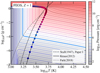 |
Fig. 2 Frankfurt equation of state. Shown are pressure contours as a function of density and temperature for a fully SiO2 composition (Z = 1). Regions where the iso-pressure contour are vertical represent phase transitions. The LV-curve by Stull (1947) (used in Paper I) is given by the dashed curve, while the colored dots indicate the experimentally inferred curve by Kraus et al. (2012); the color indicates the pressure. The fit to the Kraus et al. (2012) data (solid black curve) is used in this work as the LV-curve. |
2.4.2 Nonideal EoS
We follow the method outlined in Vazan et al. (2013) to obtain the EoS of a mixture of hydrogen, helium, and SiO2. For the H+He mixture, the SCVH EoS (Saumon et al. 1995)1 is used at a fixed helium-to-hydrogen mass ratio of Y∕X = 0.3∕0.7. For SiO2 we use the publicly available Frankfurt equation of state (FEOS; Faik et al. 2018), which uses a quotidian model (More et al. 1988) with a soft-sphere correction (Young & Corey 1995) to better represent the behavior near the critical point. We note that the SCVH EoS includes H-dissociation and ionization, whereas the SiO2 EoS only includes ionization. More generally, chemistry or interactions among materials in the mixture is not accounted for. The mixing with H+He follows the additive volume law (Vazan et al. 2013). The EoS provides us with pressure and internal energy as a function of density, temperature, and metallicity Z.
Results of the FEOS nonideal EoS (Z = 1) are shown in Fig. 2, where pressure contours are plotted as functions of temperature and density. Vertical lines indicate a phase transition between liquid and vapor: a small change in pressure is sufficient to change the density dramatically. However, beyond the critical temperature (Tc = 5100 K), a phase transition no longer takes place; the fluid becomes supercritical. Beyond the critical point, at higher densities, the spacing between the iso-pressure curves decreases considerably: a supercritical fluid is hard to compress. This behavior is markedly different from the ideal case, that is, P∕Pideal ≫ 1.
In Fig. 2, the liquid-vapor curve (LV-curve) consistent with FEOS (dotted line) differs from the expression corresponding to Stull (1947, dashed curve), which we used in Paper I. In addition, we overplot shock-and-release experimental data for the LV-curve (Kraus et al. 2012, symbols). These data can be seen to match the FEOS well (i.e., the color of the dot, indicating the pressure from the experiments, matches the color of the iso-contour from the quotidian EoS) for the lower branch (at densities below the critical point). As the parameter space traversed by the upper branch is unimportant to this work, we only fit the lower branch of the Kraus et al. (2012) LV-curve
![Mathematical equation: \begin{equation*} \rho_{\mathrm{sat,Kraus}} = \exp\left[ a -\frac{b}{T} +\left(\frac{T}{T_{\textrm{c}}} \right)^c \right],\end{equation*}](/articles/aa/full_html/2021/03/aa39706-20/aa39706-20-eq23.png) (16)
(16)
(cgs units) where a = 9.0945, b = 5.630 × 10⁴ K, c = 13.26, and Tc = 5130 K (sold curve).We fit the saturation vapor pressure with a similar expression. We consider the Kraus LV-curve – parameterized by Eq. (16) – to be the most realistic. The Stull curve is also used, in order to facilitate comparison to Paper I2. Material in excess of the LV-curve is added to the core, the density of which is assumed to be fixed.
In Fig. 3 we also present the adiabatic gradient ∇ad and internal energy uint normalized to kBT∕mu for a vapor-only Z = 1 fluid. In thisway we contrast the thermodynamical properties of the nonideal vapor with the ideal vapor gas, for which these values are about 0.18 (∇ad) and 0.075 (uint; not accounting for the energy of vaporization). As can be seen from Fig. 3 the adiabatic gradient is generally higher than ideal along the LV-curve and in the top part of this panel (these are the regions sampled by the simulations). The higher adiabatic gradient (lower compressibility) at higher pressures reflects the fact that the molecular size becomes significant and that inter-molecular interactions become important. Higher temperatures imply more vibrational modes, and hence ∇ad tends to decrease in this direction. At low densities, ionization increases the internal energies of the gas.
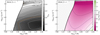 |
Fig. 3 Frankfurt equation of state: adiabatic gradient and internal energy. For clarity, only data exterior to the Kraus LV-curve are shown. The orange curve in (a) denotes the value of ∇ad in the ideal limit. For the internal energy, all values lie above the ideal limit of uint = 0.075kBT∕mu. |
2.4.3 Wet adiabat treatment
In the regions where the atmosphere becomes saturated, the density and pressure follows the LV-curve. This “wet” adiabatic gradient is therefore
 (17)
(17)
where the saturation vapor pressure Psat is fit by the same expression as Eq. (16) with a = 32.599, b = 5.701 × 10⁴, and c = 3.395. Between 3000 and 5000 K, 0.05 < ∇wet < 0.07, which are much lower than ∇ad in the ideal EoS (0.18) and the nonideal EoS. The lower adiabatic gradient arises because energy goes into sublimating the condensates at the expense of the internal energy of the vapor.
In general, the value of ∇ad will lie between the adiabatic index of a nonsaturated mixture provided by the EoS, and ∇wet. To our knowledge, analytical expressions for such a mixed ∇ad are only available in the limit where the noncondensible gas is ideal (Kasting 1988; Chambers 2017). We therefore adopt a simple weighting:
 (18)
(18)
where the weighting factor is given by w = (Pz∕Psat) × (Pz∕P). The form of Eq. (18) and the choice of w loosely follow Kasting (1988) and Chambers (2017)3. Only when the vapor is both saturated (region 1: Pz = Psat) and actually dominates the mixture (Pz = P) does the adiabatic gradient follow the wet adiabat. Conversely, when the vapor is saturated but is insignificant in terms of mass (at low temperature in region 1, Pz ≪ P) or when the vapor is no longer saturated (high temperatures of region 2, Psat ≫ Pz) we get the standard results from the mixed EoS of two gases. We find that the reduction of ∇ad in Phase I is important as it ameliorates the positive feedback effect that drives the cusps of high temperature, density, andmetallicity (Paper I and below). The wet adiabat treatment is applied in both the ideal and nonideal simulations.
2.5 Boundary equations and solution technique
We choose time t as the evolutionary parameter and increment t in such a way as to keep the relative increase in total mass limited to a few percent. The total mass Mtot is therefore an unknown parameter. The grid parameter is the internal mass m, which ranges from the core mass Mcore at the bottom of the envelope to Mtot at the outer boundary.
In total, the system consist of five differential equations, for pressure, temperature, radius, vapor mass, and energy as a function of mass m. In addition, we have the unknown parameters M and Mcore (Phase I) or Mtot and Zcnv (Phase II). In order to solve the system boundary conditions (or relations among them) must therefore be specified.
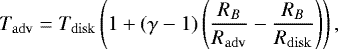
This is shown schematically in Fig. 4. At the inner boundary of the envelope, we take r = R(Mcore), where we assume that the core density is fixed at ρcore. Furthermore, E = Ecore, and mZ = Mcore are known. At the outer boundary we assume pressure and thermal equilibrium with the background disk, characterized by pressure Pdisk and temperatureT = Tdisk. The classical choice is to place the interface of disk and envelope at the minimum of the Bondi radius and the Hill radius:
 (19)
(19)
where RBondi = GMp∕γkBT and  . This closes the system of equations.
However, hydrodynamical studies indicate that the atmosphere may not be bound within the Bondi (or Hill) radius (Ormel et al. 2015; Fung et al. 2015). Instead, they hint at a complex flow pattern, where especially the outer atmosphere is continuously replenished with disk material, rendering cooling inefficient. The degree of this atmosphere–disk recycling is, unfortunately, somewhat complex, depending greatly on the ability of the gas to cool (Cimerman et al. 2017; Kurokawa & Tanigawa 2018), but the overall trend is that the outer regions are rapidly replenished, while the (very) inner regions are more prone to be bound. To encapsulate this effect in 1D evolutionary calculations, we may simply (and crudely) shift the outer radius inwards (Ali-Dib et al. 2020). Beyond this radius, Radv, the gas may be modeled as adiabatic if cooling is insignificant on an advective crossing timescale: entropy is advected (and conserved). Assuming an ideal EoS for the gas, the conditions at Radv are therefore:
 (20)
(20)
and 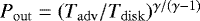 (Ali-Dib et al. 2020). In this work, for simplicity we fix Radv = 0.5Rdisk in some simulations to explore how entropy advection affects the results.
The differential equations are solved with SciPy’s integrate.solve_bvp module. The solution technique is described in previous works (Ascher et al. 1994; Kierzenka & Shampine 2001; Shampine et al. 2006). Based on an initial (or intermediate) guess for the structure, solve_bvp will calculate the residual of the numerical derivative (from the guess structure) and that of the ODE expressions of Eq. (3) for all grid points and on the boundary. solve_bvp will then adjust the solution until the residuals have become small enough. In our code, the solution structure to previous time is also available, which is needed to calculate the luminosity (see Eq. (10)). For example,
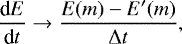 (21)
(21)
where primes denote the previous time. The energy at the previous time t′ but the present mass grid m, E′ (m), is obtained by interpolation. We note the implicit formulation; the luminosity L depends on the new structure.
At t = 0, the simulations are initialized with a core mass that is small enough to render the envelope close to isothermal, with which the analytic (isothermal) guess solution will be close to the (known) analytical solution for constant T. The precise initial value is inconsequential for further evolution. At all other times, we start from the previous solution structure or we predict the solution structure at time t by extrapolating the previous results.
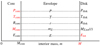 |
Fig. 4 Schematic of the numerical problem. The (independent) grid parameter m ranges from the core mass Mcore to the (unknown) total mass M. The five structure equations for P, T, r, Mz, and E are solved byimposing ten boundary conditions. The radii Rcore and Rout follow from Mcore and M, respectively, and MZ,tot is incremented according to the time-step Δt, ΔMZ,tot = ṀpebΔt. The total energy E is needed to provide the luminosity L at any point (Eq. (10)). In Phase II, Mcore becomes a known parameter, while the metallicity threshold parameter Zmax is added as an unknown. |
3 Results
We consider three disk locations, 0.2, 1, and 5 au, and four different pebble accretion rates, 10−4, 10−5, 10−6, and 10−7 M⊕ yr−1. The pebble radius, which in our model setup only affects the opacity, is varied between “None” (no additional opacity from grains) and 100 μm. Other parameters are listed in Table 1. For simplicity, it is assumed that pebbles consist of silicates. At 5 au, where the ambient disk temperature is only 150 K, it is natural to expect that pebbles also contain H2 O ice, which would ablate from the pebbles at much lower temperatures than SiO2. Therefore, our results for 5 au primarily serve to illuminate trends upon varying the physical conditions, rather than being an attempt to accurately model a particular planet (e.g., Jupiter).
Simulations are run until the crossover mass is reached. Table A.1 presents the properties of the planet and atmosphere at this point for all model runs, and lists the core mass, vapor mass of the envelope Menv,Z, the H+He mass in the envelope Mxy, the time after which crossover is reached tcross, the corresponding timescale for gas accretion (txy = Mxy∕Ṁxy, and the extent of the region where metals constitute more than 5% by mass r0.05. We also provide the average metallicity Zdc within this region (including the core), which may be considered a measure for the diluteness of the heavy metals in the central regions (dilute core). Hence, for a sharp transition between a Z = 1 core and a metal-poor envelope Zdc = 1. But in cases where vapor mixes with H+He gas, Zdc decreases, that is, within the limit that the central region is of homogeneous composition of Z* > 0.05, Zdc = Z*.
3.1 Baseline model
In Fig. 5 the density and temperature profiles of the standard model (conditions applicable to 0.2 au, real EoS with the Kraus et al. 2012 LV-curve, ṀPeb = 10−6 M⊕ yr−1, no opacity from pebbles) are provided in an evolutionary sequence. Snapshots are shown every million years and at the end when the critical metal mass is reached. Initially (t ≲ 1 Myr) the vast majority of the accreted pebbles settle to the core without significant loss to thermal ablation, which is the classical situation. The envelope can be divided into a convective interior region and a radiatively supported outer region, characterized by constant T. Nonetheless,because of the increasing temperatures near the base of the envelope, an increasingly large fraction of their mass will be lost to the envelope by ablation. This is already clear after 1 Myr (Fig. 5a) from the very steep increase in the vapor density, which follows the saturation density (Phase I).
As the saturation density is an exponential function of temperature, the regions close to the core–envelope boundary (CEB) become dominated by vapor. Because of the much higher molecular weight of the SiO2 vapor, both density and temperature shoot up, as we explained in Paper I. Still, as of 2 Myr (Fig. 5b) pebbles are only partially ablated, because the envelope’s ability to absorb is limited. However, this absorption increases with time, and a point will be reached where the pebbles sublimate completely. This marks the end of Phase I (“direct coregrowth”). Compared to Paper I we note that the transition core mass we obtain here is higher by about a factor of two, primarily because the wet adiabatic gradient we employ in this work renders this region less hot.
In Phase II, the inner envelope is characterized by two new regions: the isothermal, compositionally “frozen” zone (2b) and a convective region (2a) of constant metallicity Zcnv = ρZ∕ρ. The frozen zone emerges because there is not enough energy present to effectively mix this region. Pebbles, no longer reaching the core, deposit their energy in higher layers. Because of the rising temperatures, the interface between regions 1 and 2a moves out (in mass space), causing the metallicity of region 2a to drop as region 1 has the lower Z even though it is saturated. For region 2, most of its energy arises from the compression of the envelope. Nevertheless, it is insufficient to mix the entire region 2 to uniform Z; only the upper layers (region 2a) do. The boundary between regions 2a and 2b is indicated by the thin vertical solid line in Fig. 5. With time, this line moves outward: the frozen region (2b) becomes larger. At the same time, as more metal-free nebular gas enters the atmosphere, the metalliticy of the well-mixed region (2a) drops. The composition at a certain mass shell in region 2b is set at the time when this mass shell is transferred from 2a to 2b (crossed riso), and is frozen thereafter. As a result, a compositional gradient develops in the frozen region (2b).
As all accreted solids are turned into vapor, the total amount of vapor in the envelope steadily increases. By 5 Myr (Fig. 5e), it has exceeded the core mass. Initially (Figs. 5c,d), the envelope is vapor-dominated (MZ,env ≫ Mxy). Nevertheless, accretion of H+He gas slowly catches up with the (constant) accretion rate of pebbles. After 5 Myr (Fig. 5e), H+He gas is accreted at a higher rate than pebbles, and after 5.6 Myr (Fig. 5f) the H+He fraction has exceeded the combined mass of the core and the high-Z vapor, which is our definition of crossover. We verified that by crossover the planet accretes H+He gas on a timescale (txy = 1.9 Myr) shorter than its evolutionary time (tcross = 5.6 Myr). The planet will therefore turn into a hot-Jupiter provided the disk is able to keep supplying gas. Conversely, when the disk disperses before tcross, hot-Jupiter collapse is avoided and the planet ends up as a (mini-)Neptune planet.
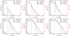 |
Fig. 5 Evolution of envelope profiles of temperature (red), total density (solid black), and vapor density (dashed solid) for the standard model (0.2 au, Ṁpeb = 10−6 M⊕ yr, FEOS with Kraus LV-curve, molecular opacities). The CEB is indicated by the vertical solid line, while the vertical dotted linesdenote the boundaries between the frozen zone (region 2b), the well-mixed region 2a, and the saturated region 1. These boundaries expand with time, creating a gradient in the composition. The radiative–convective boundary is indicated by the gray dot. The rate of gas accretion accelerates toward the end, as the crossover mass is reached. The temporal evolution is available as an online movie. |
3.2 Ideal versus real EoS
As many studies – including ours in Papers I and II – are based on an ideal EoS (e.g., Lee et al. 2014; Gupta & Schlichting 2019), we feel the need to compare our results obtained with the real EoS to the results based on the ideal EoS (Sect. 2.4.1). In Fig. 6, we contrast the time-evolution of several key quantities between thenonideal EoS runs, and in Fig. 7 we contrast the density and temperature profiles at two points in their evolution: (i) when pebbles fully evaporate (transition Phase I and II); and (ii) at the crossover mass.
In Phase I, the ideal and nonideal runs evolve similarly, because nonideal effects are unimportant for low-density atmospheres. When a vapor-dominated inner region appears, the temperature and especially the density tend to rise steeply. However, the cusps that we see in this work are less pronounced than we saw before in Papers I and II. The reason is that the adiabatic gradient transitions to that of a wet adiabat, which drives ∇ad in both the ideal and real EoS to the same value. As can be seen from Fig. 7, the profiles at the point of transition between Phase I and II are quite similar.
After reaching Phase II, there is no longer an energy source from accretion at the CEB, which mitigates the temperatureincrease or even decreases it (for the real EoS; Fig. 5). In the ideal case, the density nearthe CEB continues to increase because the ideal vapor is still characterized by the same low γad, i.e., a highly compressible vapor. Densities then start to exceed the density of the core, which is unphysical. At the point of crossover, the ideal run achieves densities of ρ = 15.5 g cm−3 at the base of the envelope, whereas this is ρ = 2.2 g cm−3 for the nonideal EoS which is still less dense than the core. In contrast, in the nonideal runs the vapor becomes supercritical and much harder to compress (see Fig. 2). Because the vapor in the ideal runs is confined to a shell immediately next to the CEB,the intake of H+He-rich material is stronger in the ideal case with respect to the nonideal EoS run and the crossover mass is somewhat smaller.
Barring the difference in the density and temperature profiles, which differ greatly in the central regions, there are no major qualitative differences between the outcome of the ideal and nonideal runs when one considers the integrated quantities at crossover (i.e., tcross, Mcore, Mcross; see Table A.1). Rather than the EoS, uncertainties pertaining to the LV-curve, (multi-species) chemistry, and dissociation (neglected here) will have far greater effects. Therefore, simulations based on the ideal EoS provide acceptable, first-order results. Still, the distribution of (vapor) density and temperature is of importance when one considers the long-term evolution of the interior structure and the potential for mixing.
Figure 7 also illustrates the effects of our implementation regarding the avoidance of negative luminosity. The vertical line indicates the dividing line between the isothermal region (2b) where the composition is frozen and the region (2a) where convection operates to mix the vapor and H+He gas to uniform Z. This distinction is reflected in the luminosity profiles. In the frozen region, PdV compression liberates energy and the luminosity increases. Conversely, in region 2a, mixing consumes energy and L decreases. The luminosity therefore peaks locally (by construction) at the interface of regions 2a and 2b.
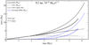 |
Fig. 6 Comparison of time-evolution between the real EoS (solid lines) and ideal EoS (dashed) standard model run (0.2 au, Ṁpeb = 10−6 M⊕ yr−1, no opacity from pebbles). The masses (total, core, metal, and H+He) are plotted on the y-axis as function of time. The points where the core mass is fixed (evolution to Phase II) are indicated by the open gray circle, while the points of crossover are indicated by the blue circles. |
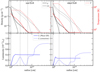 |
Fig. 7 Profiles of density, temperature, and luminosity for the simulation with the real EoS (left panels) and the ideal EoS (right panels). Parameters as in Fig. 6. Profiles are plotted just after Phase II is reached (bright curves) and after crossover (dim curves). For the state at crossover, the vertical dotted line indicates the dividing line between the isothermal region 2b, the mixed region 2a, and the saturated region 1. |
3.3 Comparison to analytical predictions
In Paper II we derived analytical formulae for conditions at crossover based on a simple three-layer model of the atmosphere. Specifically, for the crossover mass, we derived:
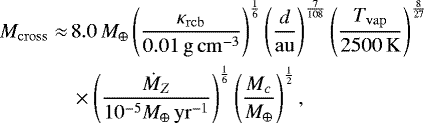 (22)
(22)
(Eq. (30) of Brouwers & Ormel 2020, the crossover mass is twice the critical metal mass) where Tvap, a parameterin the three-layer model, identifies the outer boundary of the vapor-dominated zone and κrcb is the opacity at the radiative-convective boundary.
We test Eq. (22) in Fig. 8a, where we obtain κrcb directly from our simulations (so this value is different per run) while the evaporation temperature is fixed at its fiducial value of 2500 K. The analytical prediction follows the numerical results quite well, especially given the assumptions that our analytical model contains (e.g., a fixed adiabatic index). Nevertheless, the deviation between the numerical and analytical results is not significant. Even though the nonideal runs result in higher core masses, the Mcore–Mcross relation is not affected by the choice of the EoS. This is because the relation reflects a more basic principle: core and atmosphere mass are coupled by the thermal state of the envelope. For example, a hotter envelope results in more evaporation and a smaller core mass, which give rise to a smaller crossover mass. We attribute the lower predicted crossover mass of the 0.2 au runs to the breakdown of the isothermal assumption on which Eq. (22) relies in the outer radiative region. This implies that the atmosphere mass (for a given core mass) is lower, hence the higher crossover mass.
Compared to our previous works (Papers I and II), core masses are higher because of the inclusion of a wet adiabat, as discussed above. A second reason for the higher core masses is that we are now using the Kraus et al. (2012) LV-curve, which lies below the Stull (1947) curve that we used before (see Fig. 2); for a given temperature vapor will become saturated at a lower density for the Kraus LV-curve. As a result, the value of the core mass after Phase I is typically around 1.5–2 M⊕. In Fig. 8b it can also be seen that the core masses obtained from the real EoS simulations (filled symbols) are slightly higher than those obtained from the ideal EoS simulations. The reason for this effect is that the high-density, high-temperature cusps that develop towards the end of Phase I are still somewhat more pronounced in the ideal simulations, especially in terms of density (Fig. 7) because the non-ideal vapor is less compressible4; although the effect is suppressed by the wet adiabat. The dependence of the core mass on the pebble accretion rate is ambiguous: at 5 au there is a positive trend, while at 0.2 au the trend is negative. Competing effects are at play that make this trend rather shallow. A higher Ṁpeb tends to saturate the envelope, prolonging Phase I, but it also raises the temperature, allowing more vapor to be absorbed.
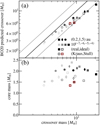 |
Fig. 8 (a) Analytically predicted (Paper II) vs. numerically-obtained crossover mass for simulations at different distances (symbols), pebble accretion rates (symbol color), and EoS (filling). The thick diagonal line indicates a perfect match (predicted=numerical) while the thin lines indicated a 50% offset. (b) Corresponding core masses. Square symbols with a brown edge color employ the Stull (1947) LV-curve. |
3.4 Benchmark test
To put these results in context, we compared our results to the classical assumption where pebbles are immune to sublimation and end up in the core. Figure 9 shows this comparison for models run at 0.2 au and for ṀZ = 10−5 M⊕ yr−1. As there is no vapor in the envelope in the classical model, the line “core” and “core+vapor” overlap. In the classical run, the core mass eventually exceeds 10 M⊕, whereas in the case with pebble sublimation it reaches just over 2 M⊕. Despite the relatively small core, the run allowing for pebble sublimation takes in a higher fraction of nebular gas, as illustrated by the slope of the blue lines (which gives Ṁxy). The reason is that (part of) the vapor mixes with the nebular gas (in region 2a) to lift the molecular weight of these parts of the envelope, reducing the local pressure scale height. To satisfy pressure balance, more nebular gas is accreted.
Figure 10 presents a more complete study, and illustrates how the results are affected by entropy advection. In this scatter plot, we show the crossover mass of 27 runs as a function of distance and pebble accretion rate (x-axis). In the case without sublimation (circles) there is by definition no Phase II and there is also no isothermal layer; the continuous accretion of pebbles onto the cores will render the luminosity positive everywhere. However, in terms of the critical metal mass, the outcome is similar to our standard runs, especially in the outer disk and for low accretion rate. This is unsurprising, because the combination of low opacities and low Ṁpeb render the envelope so cold that pebbles hardly sublimate (see the last two lines of Table A.1 and note the low MZ,env). On the other hand, in the inner disk runs, where pebbles vaporize, the vapor and associated higher molecular weight of the atmosphere accelerates the intake of H+He gas, because the mixing results in a more compressed envelope (Paper II).
At 5 au, we can compare our results to those of Hori & Ikoma (2010), who consider almost exactly the same parameters in their study. The critical core masses that they obtain are approximately, 2, 3, and 5 M⊕, respectively,for the three accretion rates. These numbers are slightly higher than ours, but not significantly so. The critical core mass in their study may be slightly higher than half the crossover mass, as it is set by the failure of hydrostatic balance. More generally, these results are relatively sensitive to the opacity model, for which we have used simple power laws5.
In the runs with entropy advection (triangles), the atmosphere is 50% smaller in radius (see Sect. 2.5). The layer between Radv and Rdisk is assumed to have the same entropy as the disk (the layer is not included in the envelope mass) and therefore the density at Radv will be lower and the temperature higher. Consequently, the atmospheres tend to have less H+He for a given metal mass, resulting in a higher crossover mass. Another feature is that gas accretion rates at crossover are not very high, txy ~ tcross, especially for the inner regions. This suggests that these atmospheres have not yet entered runaway gas accretion. Otherwise, for all other runs, the critical metal mass always signifies the onset of runaway gas accretion.
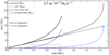 |
Fig. 9 Temporal evolution of two runs with our (standard) choice of evaporation (solid) and for the classical choice where solids end up in the core (dashed). Other parameter are the same (e.g., ṀZ = 10−5 M⊕ yr−1). Due to the absorption of vapor by the envelope and the concomitant reduction of the local pressure scaleheight, the intake of nebular gas (Mxy) speeds up in the run where pebbles sublimate. |
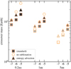 |
Fig. 10 Comparison of our standard model setup (squares) with other model designs: sublimation-free runs (all solids reach the core; circles) and runs with entropy advection (triangles) as a function of distance and pebble accretion rate (x-axis). The symbol filling indicates the level of pollution of the atmospheres at the point of crossover (white: no vapor; black: 50% vapor). The symbol border color indicates how quickly nebular gas is being accreted (black: txy ∕tcross ≥ 1; copper: txy∕tcross = 0). See Table A.1 for the precise values. |
3.5 Opacity of pebbles
Until now we have assumed a grain-free atmosphere. This assumption is based on the belief that any grains that would co-accrete with the gas would readily coagulate and be removed by settling (Mordasini 2014; Ormel 2014). In addition, one can argue that many of the “original” grains have been converted into pebbles, planetesimals, or planets, rendering the abundance (much) lower than the ISM value (~ 10−2) and also highly uncertain. Conversely, pebbles are accreted at a rate Ṁpeb, an input parameter that can be straightforwardly converted into an opacity by Eq. (6) once we specify a pebble size. This value is then added to the molecular opacity.
Figure 11 presents the crossover mass as a function of pebble size (symbol), distance (x-axis), and accretion rate (x-axis). Large pebbles, simulations conducted in the inner disk regions, and simulations at low Ṁpeb do not significantly deviate from the grain-free result (squares; grain-free meaning no opacity from solids). In the inner regions, the molecular opacity is much higher and the pebbles contributes little. Conversely, in the outer disk a smaller pebble size and a higher pebble accretion rate enhance the pebble opacity, rendering atmospheres hotter and less dense. When pebbles dominate the opacity, we find that the crossover mass becomes much higher. For example, at 5 au for Ṁpeb = 10−6 M⊕ yr−1, the crossover mass jumps from ≈3M⊕ (grain free/1cm size pebbles) to ≈ 7 M⊕ (1 mm pebbles) to 22 M⊕ (100 μm pebbles). A similar effect is seen for the accretion rate: at 5 au for 1 mm pebbles, the crossover mass scales as 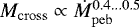 . Furthermore, when pebbles dominate the opacity, the crossover mass tends to become independent of distance. The key reason is that κpeb is independent of gas density: r2vsed = GMtstop (force balance) and r2vsedρgasspeb is therefore approximately constant in the Epstein limit (see Eq. (6)).
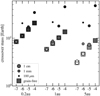 |
Fig. 11 Dependence of crossover mass on pebble size. A different pebble size changes the opacity. “Grain-free” indicates that pebbles do not contribute to the opacity. The symbol filling indicates the level of enrichment of the atmosphere at crossover (white: no vapor; black: 50% vapor). |
3.6 Phase III
In all preceding simulations, we assumed a continuous and constant flux of pebbles up to the crossover mass. In reality, it is conceivable that the pebble flux will stall, for example when the disk has run out of pebble-building material, an exterior giant planet forms and stops the pebble flux interior to it, or when the planet itself has has reached either the pebble isolation mass (Ataiee et al. 2018; Bitsch et al. 2018) or the flow isolation mass (Rosenthal & Murray-Clay 2020; Kuwahara & Kurokawa 2020, for small pebbles). In these cases, the evolution is set by the self-contraction of the envelope (Phase III). We therefore run a suite of simulations where we set the final solid mass MZ,final at 4, 6, and 8 M⊕, respectively,as described in Sect. 2.1.3.
Figure 12 shows the total planet mass (metals and gas) as a function of time for these runs, including the standard run with unlimited pebble supply (Mz,final = ∞; left-most branches). The (initial) pebble accretion rate is Ṁpeb = 10−5 M⊕ yr−1. Two runs are shown, one assuming grain-free envelopes (applicable for large pebbles; green) and another with additional opacity from speb = 1 mm pebbles (blue).
As discussed in the previous sections, runs with an additional opacity contribution from pebbles reach higher crossover masses. However, when the pebble accretion shuts off after M ≈ MZ,final (dashed horizontal lines; the total planet mass is dominated by metals at this point), the envelopes will nonetheless become grain-free, greatly reducing the opacity, especially in the outer disk. Consequently, these envelopes start to cool more rapidly. Accretion of metals (black) gives way to accretion of H+He gas (color). The reason is simply that the Kelvin-Helmholtz timescale is short for grain-free atmospheres. Only when pebble accretion is halted at MZ,final = 4M⊕ at 0.2 au do we observe a transition to a slower evolutionary growth. The reason is that tKH is a strong function of both opacity and planet mass (Hori & Ikoma 2010; Lee et al. 2014).
While our numerical results for Phase II broadly agree with the analytical predictions of Paper II, this no longer applies to Phase III. In Paper II we assumed that the composition of the vapor-dominated part of the envelope stayed homogeneous. Therefore, we argued that with addition of H+He gas and subsequent reduction in the molecular weight, the gas provided more hydrostatic support. Consequently, our prediction was that gas accretion would slow. However, in reality there is not enough energy to fully mix the vapor-rich regions with the incoming H+He gas: a caveat that we already addressed in Paper II.
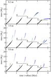 |
Fig. 12 Simulations where the total mass of accreted pebbles is limited to (from left to right): MZ,final = ∞ (unlimited; left), 8, 6, and, 4 M⊕ (right). Plotted is the total planet mass against time. Simulations terminate at crossover. Blue curves correspond to runs with additional opacity from mm-sized pebbles (the pebble opacity vanishes along with pebble influx). Green curves correspond to runs with only molecular opacities. The color indicates the nature of the accretion material, ranging from dominated by pebbles (black) to being dominated by nebular gas (blue or green). |
3.7 The interior metal distribution
During Phase II the inner atmosphere is highly polluted, characterized by a high, super-solar metallicity. The extent of this region becomes more apparent when we plot profiles as a function of mass instead of radius. In Fig. 13 the metallicity and temperature profiles are plotted for several runs conducted at 0.2 au at three points during their evolution where the total mass reaches 5, 10, and 20 M⊕. In these figures, the classical core, identified by Z = 1, starts at m = 0 while the remainder of the mass is dominated by the isothermal region 2b and the iso-metal region 2a, before a sharp drop-off in the metallicity in region 1. The temperature profile of the “classical” core (where Z = 1, indicated in light red) reflects the values at the base of the envelope when the material became incorporated in Phase I. Because heat is not being transported or generated in the core in our model, this temperature profile does not affect the surrounding envelope.
In Fig. 13, the extent and value of the average metallicity over the regions where Z > 0.05 – which is our definition of a dilute core – is indicated by the horizontal dashed line. It is clear that with this definition the entire region 2 has become an extension of the core. We can expect that hotter envelopes are less dense, more polluted, and have therefore higher Zdc values. In Fig. 13 we observe this trend at fixed total mass. For example, in the middle column panels (M = 5 M⊕) higher ṀP and κ leads to higher temperatures and higher Zdc. Naturally, the dilute core metallicity Zdc decreases with time as the convective region (2a) progresses outward and its metallicity decreases, reaching ≈0.5 at crossover for the Ṁpeb = 10−5 M⊕ yr−1 runs. At crossover, Zdc = 0.5 is the lowest value that can be attained, because it implies that the dilute core encompasses the entire envelope. In Table A.1, we list the value of Zdc for all runs. As can be seen from Table A.1, runs where significant vapor layers have built up reach Zdc ≈ 0.5 at crossover, indicating that pebble accretion naturally produces a dilute core with an approximately 1:1 ratio between heavy metals and H+He gas.
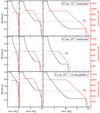 |
Fig. 13 Metallicity and temperature profiles for several runs at 0.2 au: with an accretion rate of Ṁpeb = 10−5 M⊕ yr−1 (top); a lower accretion rate of Ṁpeb = 10−6 M⊕ yr−1 (center); and a pebble opacity corresponding to mm-sized pebbles (bottom). Profiles are shown when M = 5, 10, and 20 M⊕ are reached (unless crossover is reached sooner). The value of the diluted core Zdc – defined as the average over the region where Z > 0.05 – is also indicated. The temperature in the classical core region, which is not modeled, indicates the temperature at the CEB when the material was incorporated. |
4 Discussion
4.1 The dilute core
Recent analyses of Jupiter’s gravitational moments as measured by the Juno spacecraft indicate that Jupiter’s central region is best characterized by a modest metallicity, which gradually transitions into the H+He-dominated envelope – the dilute core – rather than a sharp interface between a fully metal core and a near metal-free envelope (Wahl et al. 2017; Debras & Chabrier 2019). Sublimationof solids during assembly naturally reproduces this trend and the region where the heavy metal fraction exceeds 5% is substantial. Still, this fraction may not reach the levels as inferred from Juno, which seem to indicate a dilute core metallicity as low as Zdc ≈ 0.3 (Wahl et al. 2017; Liu et al. 2019). Liu et al. (2019) explain Jupiter’s dilute core by means of an (head-on) impact of Jupiter’s core with an embryo. Pebble accretion may offer an alternative or additional explanation. In this work, simulations end at crossover; we have not accounted for the effects of additional planetesimal accretion (Venturini & Helled 2020) or for the runaway gas accretion and circumplanetary disk accretion phases, which may contribute to further solid accretion (Szulágyi et al. 2018; Cilibrasi et al. 2018; Shibata & Ikoma 2019; Shibaike et al. 2019; Podolak et al. 2020), and have not modeled the interior profiles for billions of years. Redistribution of vapor by mixing, for example due to a Ledoux-unstable configuration or miscibility of the core in metallic hydrogen (Wilson & Militzer 2012; Soubiran et al. 2017), or settling, will affect Zdc and the gravitational moments (Müller et al. 2020).
In addition, planets that have not reached crossover – (mini-)Neptunes – will also be characterized by extended vapor regions after their formation. Although we did not consider ices, a gradual composition can also explain the measured properties of the ice-giants of the Solar System (Marley et al. 1995; Podolak et al. 2000; Helled et al. 2011; Vazan & Helled 2020). At any rate, our works provide the (realistic) profiles that emerge from the planet formation process by pebble accretion until crossover (Fig. 13); interior structure calculations can use these in their post-formation calculations to assess the long-term stability and evolution.
4.2 Preservation of (sub)-Neptune planets
One of the motivations for this study is to explain the presence of H+He-rich, but heavy-metal-dominant close-in planets – sub-Neptunes – from a pebble accretion perspective. Because of the inferred H+He envelopes, it is natural to assume that these planets were formed within the gaseous disk. The challenge, then, is to understand why these planets stopped at sub-Neptune sizes and did not become hot-Jupiters. Delaying contraction by accretion of remnant planetesimals, as recently proposed for Jupiter (Alibert et al. 2018; Guilera et al. 2020), is not applicable at ~0.1 au as these bodies are accreted on very short timescales. Another line of thinking is that these planets simply ran out of gas to accrete, because they formed late (e.g., Lee & Chiang 2016; Ogihara et al. 2020), the gas disks dispersed by photoevaporation, or because of inefficient accretion due to gap opening (Tanigawa & Ikoma 2007; Ginzburg & Chiang 2019; Venturini et al. 2020).
Most of the proposed solutions assume that atmospheres are dusty, which naturally prolongs the Kelvin-Helmholtz contraction. Here, we have adopted the opposite limit of entirely grain-free atmospheres. Our Phase III simulations and previous analytical work then indicate that the critical metal mass is reached already at ≈5 M⊕ (at 0.2 au) and much less further out.
Pebbles affect gas accretion in two ways. On the one hand, they accelerate gas accretion through accumulation of a vapor-rich atmosphere, which brings down the crossover mass by a couple of Earth masses. Similar to the findings by Valletta & Helled (2020) for H2 O polluters, intake of nebular gas becomes significant before the pebble isolation mass is reached. Conversely, by virtue of their small size, pebbles naturally provide an opacity, which reduces the intake of nebular gas. However, this pebble opacity is most relevant for the outer disk, as there the molecular opacity is low. When pebbles are small, <1 mm, their contribution to κ significantly raises the crossover mass (see Fig. 11). At ~0.2 au, the opacity from pebbles could in principle delay gas accretion, but the window is rather narrow. The pebbles must be small, stay small (avoid coagulation) and the supply of pebbles must be uninterrupted. Otherwise, as we have seen in Fig. 12, atmospheres will quickly contract. Because at ~0.1 au disk flows are strong both in terms of density and velocity, entropy advection or entire disk–atmosphere recycling appear to us the most natural mechanism through which mini-Neptunes can retain their atmospheres (Ormel et al. 2015; Fung et al. 2015; Cimerman et al. 2017; Lambrechts & Lega 2017; Kurokawa & Tanigawa 2018; Béthune & Rafikov 2019; Moldenhauer et al. 2021).
4.3 Importance of dust collision model
Assigning a pebble opacity in the form of Eq. (6) is attractive because it can be directly linked to the pebble accretion rate and eliminates the need for an otherwise uncertain grain reduction factor. However, Eq. (6) is only applicable when it is assumed that pebbles preserve their sizes. A motivation for this simple choice is that bouncing, among silicates, seems to be primarily a size-dependent phenomenon, as deduced from laboratory experiments among silicate particles (Weidling et al. 2009; Güttler et al. 2010; Zsom et al. 2010). Nevertheless, as the opacity is perhaps the single-most important factor in determining the evolutionary outcome, it is warranted to pursue a more sophisticated collisional process. Fragmentation and erosive collisions, either in the nebula (Chen et al. 2020) or in the envelope (Ali-Dib & Thompson 2020; Johansen & Nordlund 2020), may contribute to (dominating) dust opacity, but this trend will be strongly mediated by coagulation and sedimentation (Dullemond & Dominik 2005; Mordasini 2014; Ormel 2014). In an accompanying work we provide a more general opacity model by accounting for a fine-grain dust component, dust-pebble sweep-up, and coagulation (Brouwers et al. 2020).
4.4 Comparison to related works
We briefly compare our work with that of Bodenheimer et al. (2018), who also accounted for the absorption of metal vapor in the envelope and of planetesimal accretion. A side-by-side comparison cannot be made because Bodenheimer et al. (2018) optimized their model towards understanding the properties of Kepler-36 c (at present), while we conduct a controlled parameter exploration to arrive at more general trends and conclusions.
Still, Bodenheimer et al. (2018) also end up with a core mass of between 1 and 2 M⊕, consistent with our results. However, in their case, the subsequent buildup of a vapor layer (which we refer to as Phase II) is seen to suppress accretion of nebular gas, whereas in our model it is accelerated (see Fig. 9). We attribute this difference to the fact that, in the work of Bodenheimer et al. (2018), the vapor-rich layer is shielded from the remainder of the envelope. In their setup, planetesimals release their vapor in this layer (ablation being negligible). Therefore, the high-Z vapor layer essentially acts as a low-density extension of the core, with the “inflated” core suppressing intake of nebular gas. In contrast, in our work the vapor is deposited much higher in the envelope and naturally mixes with the rest of the envelope (in region 2a) as long as the overall luminosity stays positive. The higher molecular weight compresses these layers (the pressure gradient decreases), accelerating the intake of nebular gas as was shown by Hori & Ikoma (2011) and Venturini et al. (2016) in case of H2 O. But whereas these works assume a globally constant enrichment throughout the envelope, deposition of silicate vapor in our case occurs much deeper in the envelope (see Fig. 1).
4.5 Model caveats and improvements
One of the key features of our evolution model is the onset of an inner compositionally frozen layer, which we model as isothermal. The motivation for this layer is physical; it stems from the fact that an insufficient amount of energy is available to lift the metal-rich lower layer with the metal-poor regions above. However, our choice to model this layer as isothermal is partly driven by the limitations of our numerical method. To proceed towards a more realistic treatment, a local model for energy transport (luminosity) as well as material transport (composition) is necessary. One approach for this is to opt for a pure local treatment for material and heat transport based on the Ledoux convection criterion and mixing length theory. However, the Ledoux criterion only sets a lower bound for heat transport; when it indicates stability, which the Schwarzschield criterion does not, the region is dynamically stable but vibrationally unstable. Formally, a double-diffusion convection (DDC) model should be invoked (Mirouh et al. 2012; Leconte & Chabrier 2012; Wood et al. 2013). Including DDC in the models requires knowledge of thermodynamical properties, which are poorly known (Prandtl number, diffusivity ratio, number of layers) for forming planets, which may affect the resulting interior structure.
In addition, interaction between core and inner envelope must be considered. In our model we have followed the classical choice that core and envelope are decoupled both thermally and materially. However, at these high densities and temperatures conduction may become relevant (Umemoto et al. 2006; Stamenković et al. 2011) and hydrogen from the envelope can be sequestered in the core (Kite et al. 2019).
Another major limitation is the choice of a single species: SiO2. Even though a realistic EoS was employed, it lacked dissociation (Melosh 2007). Inclusion of other volatile and metal species and their chemistry is necessary. In the outer disk, pebbles are expected to contain significant fractions of H2 O ice, which will sublimate at much lower temperatures than SiO2. While the current consensus is of a 50-50 refractory-to-volatile split for pebbles beyond the iceline (Lodders 2003; Morbidelli et al. 2015), the precise composition of the material that first accreted onto, for example, Jupiter is unknown. In addition, the rock-to-ice fraction may well vary among disks (Bitsch & Battistini 2020). Finally, when Jupiter formed near the iceline and ice sublimated readily in the outermost layer of the envelope, the H2 O vapor may have simply been advected back through the recycling mechanism (Ormel et al. 2015; Fung et al. 2015). Our assumption of a H2 O vapor-free model for the 5 au runs, while far from ideal, is not without merit.
Conversely, more refractory rock species such as MgO sublimate at higher temperatures (Haynes 2014). Conceivably, this may result in an onion-like structure where volatiles readily sublimate and reach Phase II (sub-saturation), whereas the metal species are still accreting onto the core. Within the framework of the model, it is straightforward to add additional species by following additional saturation vapor curves and using the ideal EoS. However, nonideal effects, as well as chemical interactions between the different Z species, are expected to affect the calculation and therefore require a proper description. These effects are only beginning to be treated by modelers (e.g., Hori & Ikoma 2011; Haldemann et al. 2020) and we hope to address these topics in future work.
5 Conclusions
We have extended our results of Paper I, employing a real EoS and an updated LV-curve. The results for the first phase of direct core growth are similar, although our new calculations produce larger cores. The numerical calculations now proceed to the next phase, where the accreting pebbles fully evaporate until the point where the crossover mass is reached.
Our main findings are the following:
- 1.
The critical metal mass, that is, the mass where the total mass in metals (core and envelope vapor) is equal to that of the H+He gas, heralds the onset of runaway gas accretion. We also numerically verfied other findings based on (semi-)analytical arguments and on the ideal EoS. The Mcore–Mcrossover relation closely follows the expression derived in Paper II.
- 2.
The typical core mass that we find is around 1.5–2 M⊕. This is slightly higher than that found in Papers I and II and is primarily a consequence of the wet-adiabatic gradient we employed as well as a different LV-curve.
- 3.
Temperature and metallicity profiles differ significantly between the ideal and nonideal EoS runs. As the long-term, post-formation interior evolution of planets is sensitive to these profiles, planet formation scenarios (e.g., by pebble accretion) can be linked to the present state.
- 4.
The complete vaporization of pebbles naturally enriches the atmosphere in heavy elements. Based on elementary energy considerations, the dense, heavy metal layer may only partially mix with the H+He gas. Consequentially, a compositional gradient naturally forms. Typically, the dilute core metallicity approaches Zdc ≈ 0.5 upon reaching crossover.
- 5.
In the outer disk regions, where the molecular opacity is low, small pebbles dominate the opacity. When, in addition, the pebble accretion rate is high, atmospheres become very polluted. The crossover mass becomes large and its value becomes independent of distance.
- 6.
When planets stop accreting pebbles (Phase III), accretion of nebular gas quickly takes over as the atmospheres loose their opacity. We therefore consider entropy advection or full-scale atmosphere recycling a more viable mechanism to prevent sub-Neptunes from reaching runaway gas accretion.
Movie
Movie 1 associated with Fig. 5 Access Supplementary Material
Acknowledgements
We thank the referee for a helpful report. We emphatically thank all participating members of the International Space Science Institute (ISSI) team “Ice giants: formation, evolution and link to exoplanets” for fruitful discussions. This work has benefited from the matplotlib (Hunter 2007), numpy (Harris et al. 2020), and scipy (Virtanen et al. 2020) open source software packages.
Appendix A Additional table
Conditions at crossover when the total mass is twice the mass in H+He gas in the envelope Mxy and also (by definition) twice the combined mass in heavy metals in the core Mcore and envelope MZ,env.
References
- Ali-Dib, M., & Thompson, C. 2020, ApJ, 900, 96 [NASA ADS] [CrossRef] [Google Scholar]
- Ali-Dib, M., Cumming, A., & Lin, D. N. C. 2020, MNRAS, 494, 2440 [Google Scholar]
- Alibert, Y., Venturini, J., Helled, R., et al. 2018, Nat. Astron., 2, 873 [NASA ADS] [CrossRef] [Google Scholar]
- Ascher, U. M., Mattheij, R. M. M., & Russell, R. D. 1994, Numerical Solution of Boundary Value Problems for Ordinary Differential Equations (New Jersey: Prentice Hall), 13 [Google Scholar]
- Ataiee, S., Baruteau, C., Alibert, Y., & Benz, W. 2018, A&A, 615, A110 [NASA ADS] [CrossRef] [EDP Sciences] [Google Scholar]
- Bell, K. R., & Lin, D. N. C. 1994, ApJ, 427, 987 [NASA ADS] [CrossRef] [Google Scholar]
- Béthune, W., & Rafikov, R. R. 2019, MNRAS, 488, 2365 [Google Scholar]
- Bitsch, B., & Battistini, C. 2020, A&A, 633, A10 [CrossRef] [EDP Sciences] [Google Scholar]
- Bitsch, B., Lambrechts, M., & Johansen, A. 2015, A&A, 582, A112 [NASA ADS] [CrossRef] [EDP Sciences] [Google Scholar]
- Bitsch, B., Lambrechts, M., & Johansen, A. 2018, A&A, 609, C2 [CrossRef] [EDP Sciences] [Google Scholar]
- Bodenheimer, P., Stevenson, D. J., Lissauer, J. J., & D’Angelo, G. 2018, ApJ, 868, 138 [NASA ADS] [CrossRef] [Google Scholar]
- Brouwers, M. G., & Ormel, C. W. 2020, A&A, 634, A15 [Google Scholar]
- Brouwers, M. G., Vazan, A., & Ormel, C. W. 2018, A&A, 611, A65 [NASA ADS] [CrossRef] [EDP Sciences] [Google Scholar]
- Brouwers, M. G., Ormel, C. W., Bonsor, A., & Vazan, A. 2020, A&A submitted [Google Scholar]
- Chabrier, G., Mazevet, S., & Soubiran, F. 2019, ApJ, 872, 51 [NASA ADS] [CrossRef] [Google Scholar]
- Chambers, J. 2017, ApJ, 849, 30 [NASA ADS] [CrossRef] [Google Scholar]
- Chen, Y.-X., Li, Y.-P., Li, H., & Lin, D. N. C. 2020, ApJ, 896, 135 [CrossRef] [Google Scholar]
- Chiang, E., & Laughlin, G. 2013, MNRAS, 431, 3444 [Google Scholar]
- Cilibrasi, M., Szulágyi, J., Mayer, L., et al. 2018, MNRAS, 480, 4355 [NASA ADS] [Google Scholar]
- Cimerman, N. P., Kuiper, R., & Ormel, C. W. 2017, MNRAS, 471, 4662 [Google Scholar]
- Coleman, G. A. L., Papaloizou, J. C. B., & Nelson, R. P. 2017, MNRAS, 470, 3206 [NASA ADS] [CrossRef] [Google Scholar]
- D’Angelo, G., & Podolak, M. 2015, ApJ, 806, 203 [NASA ADS] [CrossRef] [Google Scholar]
- Debras, F., & Chabrier, G. 2019, ApJ, 872, 100 [NASA ADS] [CrossRef] [Google Scholar]
- Dullemond, C. P., & Dominik, C. 2005, A&A, 434, 971 [NASA ADS] [CrossRef] [EDP Sciences] [Google Scholar]
- Faik, S., Tauschwitz, A., & Iosilevskiy, I. 2018, Comput. Phys. Commun., 227, 117 [NASA ADS] [CrossRef] [Google Scholar]
- Ferguson, J. W., Alexander, D. R., Allard, F., et al. 2005, ApJ, 623, 585 [Google Scholar]
- Freedman, R. S., Lustig-Yaeger, J., Fortney, J. J., et al. 2014, ApJS, 214, 25 [NASA ADS] [CrossRef] [Google Scholar]
- Fressin, F., Torres, G., Charbonneau, D., et al. 2013, ApJ, 766, 81 [NASA ADS] [CrossRef] [Google Scholar]
- Fulton, B. J., Petigura, E. A., Howard, A. W., et al. 2017, AJ, 154, 109 [Google Scholar]
- Fung, J., Artymowicz, P., & Wu, Y. 2015, ApJ, 811, 101 [Google Scholar]
- Ginzburg, S., & Chiang, E. 2019, MNRAS, 487, 681 [Google Scholar]
- Guilera, O. M., Sándor, Z., Ronco, M. P., Venturini, J., & Miller Bertolami, M. M. 2020, A&A, 642, A140 [CrossRef] [EDP Sciences] [Google Scholar]
- Guillot, T., Chabrier, G., Gautier, D., & Morel, P. 1995, ApJ, 450, 463 [NASA ADS] [CrossRef] [Google Scholar]
- Gupta, A., & Schlichting, H. E. 2019, MNRAS, 487, 24 [Google Scholar]
- Güttler, C., Blum, J., Zsom, A., Ormel, C. W., & Dullemond, C. P. 2010, A&A, 513, A56 [NASA ADS] [CrossRef] [EDP Sciences] [Google Scholar]
- Haldemann, J., Alibert, Y., Mordasini, C., & Benz, W. 2020, A&A, 643, A105 [NASA ADS] [CrossRef] [EDP Sciences] [Google Scholar]
- Hansen, B. M. S. 2009, ApJ, 703, 1131 [NASA ADS] [CrossRef] [Google Scholar]
- Harris, C. R., Millman, K. J., van der Walt, S. J., et al. 2020, Nature, 585, 357 [CrossRef] [PubMed] [Google Scholar]
- Haynes, W. M. 2014, CRC Handbook of Chemistry and Physics (Boca Raton: CRC Press) [Google Scholar]
- Helled, R., Anderson, J. D., Podolak, M., & Schubert, G. 2011, ApJ, 726, 15 [Google Scholar]
- Hori, Y., & Ikoma, M. 2010, ApJ, 714, 1343 [NASA ADS] [CrossRef] [Google Scholar]
- Hori, Y., & Ikoma, M. 2011, MNRAS, 416, 1419 [NASA ADS] [CrossRef] [Google Scholar]
- Hubickyj, O., Bodenheimer, P., & Lissauer, J. J. 2005, Icarus, 179, 415 [NASA ADS] [CrossRef] [Google Scholar]
- Hunter, J. D. 2007, Comput. Sci. Eng., 9, 90 [NASA ADS] [CrossRef] [Google Scholar]
- Iaroslavitz, E.,& Podolak, M. 2007, Icarus, 187, 600 [NASA ADS] [CrossRef] [Google Scholar]
- Ikoma, M., Nakazawa, K., & Emori, H. 2000, ApJ, 537, 1013 [NASA ADS] [CrossRef] [Google Scholar]
- Johansen, A., & Lambrechts, M. 2017, Ann. Rev. Earth Planet. Sci., 45, 359 [NASA ADS] [CrossRef] [Google Scholar]
- Johansen, A., & Nordlund, Å. 2020, ApJ, 903, 102 [NASA ADS] [CrossRef] [Google Scholar]
- Kasting, J. F. 1988, Icarus, 74, 472 [NASA ADS] [CrossRef] [PubMed] [Google Scholar]
- Kierzenka, J., & Shampine, L. F. 2001, ACM Trans. Math. Softw., 27, 299 [CrossRef] [Google Scholar]
- Kippenhahn, R., & Weigert, A. 1990, Stellar Structure and Evolution (Heidelberg: Springer) [Google Scholar]
- Kite, E. S., Fegley, B., Jr., Schaefer, L., & Ford, E. B. 2019, ApJ, 887, L33 [Google Scholar]
- Kraus, R. G., Stewart, S. T., Swift, D. C., et al. 2012, J. Geophys. Res. Planets, 117, E09009 [NASA ADS] [CrossRef] [Google Scholar]
- Kurokawa, H., & Tanigawa, T. 2018, MNRAS, 479, 635 [Google Scholar]
- Kuwahara, A., & Kurokawa, H. 2020, A&A, 633, A81 [NASA ADS] [CrossRef] [EDP Sciences] [Google Scholar]
- Lambrechts, M., & Johansen, A. 2012, A&A, 544, A32 [CrossRef] [EDP Sciences] [Google Scholar]
- Lambrechts, M., & Lega, E. 2017, A&A, 606, A146 [NASA ADS] [CrossRef] [EDP Sciences] [Google Scholar]
- Lambrechts, M., Johansen, A., & Morbidelli, A. 2014, A&A, 572, A35 [NASA ADS] [CrossRef] [EDP Sciences] [Google Scholar]
- Lambrechts, M., Morbidelli, A., Jacobson, S. A., et al. 2019, A&A, 627, A83 [NASA ADS] [CrossRef] [EDP Sciences] [Google Scholar]
- Leconte, J., & Chabrier, G. 2012, A&A, 540, A20 [NASA ADS] [CrossRef] [EDP Sciences] [Google Scholar]
- Ledoux, P. 1947, ApJ, 105, 305 [NASA ADS] [CrossRef] [Google Scholar]
- Lee, E. J., & Chiang, E. 2015, ApJ, 811, 41 [Google Scholar]
- Lee, E. J., & Chiang, E. 2016, ApJ, 817, 90 [Google Scholar]
- Lee, E. J., Chiang, E., & Ormel, C. W. 2014, ApJ, 797, 95 [Google Scholar]
- Liu, S.-F., Hori, Y., Müller, S., et al. 2019, Nature, 572, 355 [CrossRef] [Google Scholar]
- Lodders, K. 2003, ApJ, 591, 1220 [Google Scholar]
- Lopez, E. D., & Fortney, J. J. 2014, ApJ, 792, 1 [NASA ADS] [CrossRef] [Google Scholar]
- Lozovsky, M., Helled, R., Rosenberg, E. D., & Bodenheimer, P. 2017, ApJ, 836, 227 [NASA ADS] [CrossRef] [Google Scholar]
- Marley, M. S., Gómez, P., & Podolak, M. 1995, J. Geophys. Res., 100, 23349 [NASA ADS] [CrossRef] [Google Scholar]
- Melosh, H. J. 2007, Meteorit. Planet. Sci., 42, 2079 [NASA ADS] [CrossRef] [Google Scholar]
- Mirouh, G. M., Garaud, P., Stellmach, S., Traxler, A. L., & Wood, T. S. 2012, ApJ, 750, 61 [NASA ADS] [CrossRef] [Google Scholar]
- Moldenhauer, T. W., Kuiper, R., Kley, W., & Ormel, C. W. 2021, A&A, 646, L11 [NASA ADS] [CrossRef] [EDP Sciences] [Google Scholar]
- Morbidelli, A., Lambrechts, M., Jacobson, S., & Bitsch, B. 2015, Icarus, 258, 418 [NASA ADS] [CrossRef] [Google Scholar]
- Mordasini, C. 2014, A&A, 572, A118 [NASA ADS] [CrossRef] [EDP Sciences] [Google Scholar]
- Mordasini, C., Alibert, Y., Klahr, H., & Henning, T. 2012, A&A, 547, A111 [NASA ADS] [CrossRef] [EDP Sciences] [Google Scholar]
- Mordasini, C., Mollière, P., Dittkrist, K.-M., Jin, S., & Alibert, Y. 2015, Int. J. Astrobiol., 14, 201 [CrossRef] [Google Scholar]
- More, R. M., Warren, K. H., Young, D. A., & Zimmerman, G. B. 1988, Phys. Fluids, 31, 3059 [NASA ADS] [CrossRef] [Google Scholar]
- Movshovitz, N., Bodenheimer, P., Podolak, M., & Lissauer, J. J. 2010, Icarus, 209, 616 [Google Scholar]
- Müller, S., Helled, R., & Cumming, A. 2020, A&A, 638, A121 [CrossRef] [EDP Sciences] [Google Scholar]
- Ogihara, M., Kunitomo, M., & Hori, Y. 2020, ApJ, 899, 91 [NASA ADS] [CrossRef] [Google Scholar]
- Ormel, C. W. 2014, ApJ, 789, L18 [Google Scholar]
- Ormel, C. W., & Klahr, H. H. 2010, A&A, 520, A43 [NASA ADS] [CrossRef] [EDP Sciences] [Google Scholar]
- Ormel, C. W., & Min, M. 2019, A&A, 622, A121 [NASA ADS] [CrossRef] [EDP Sciences] [Google Scholar]
- Ormel, C. W., Shi, J.-M., & Kuiper, R. 2015, MNRAS, 447, 3512 [Google Scholar]
- Owen, J. E., & Wu, Y. 2016, ApJ, 817, 107 [NASA ADS] [CrossRef] [Google Scholar]
- Owen, J. E., & Wu, Y. 2017, ApJ, 847, 29 [Google Scholar]
- Petigura, E. A., Marcy, G. W., & Howard, A. W. 2013, ApJ, 770, 69 [NASA ADS] [CrossRef] [Google Scholar]
- Pinhas, A., Madhusudhan, N., & Clarke, C. 2016, MNRAS, 463, 4516 [NASA ADS] [CrossRef] [Google Scholar]
- Piso, A.-M. A., & Youdin, A. N. 2014, ApJ, 786, 21 [NASA ADS] [CrossRef] [Google Scholar]
- Podolak, M., Pollack, J. B., & Reynolds, R. T. 1988, Icarus, 73, 163 [NASA ADS] [CrossRef] [Google Scholar]
- Podolak, M., Podolak, J. I., & Marley, M. S. 2000, Planet. Space Sci., 48, 143 [NASA ADS] [CrossRef] [Google Scholar]
- Podolak, M., Haghighipour, N., Bodenheimer, P., Helled, R., & Podolak, E. 2020, ApJ, 899, 45 [NASA ADS] [CrossRef] [Google Scholar]
- Pollack, J. B., Hubickyj, O., Bodenheimer, P., et al. 1996, Icarus, 124, 62 [NASA ADS] [CrossRef] [Google Scholar]
- Rafikov, R. R. 2006, ApJ, 648, 666 [Google Scholar]
- Rosenblum, E., Garaud, P., Traxler, A., & Stellmach, S. 2011, ApJ, 731, 66 [NASA ADS] [CrossRef] [Google Scholar]
- Rosenthal, M. M., & Murray-Clay, R. A. 2020, ApJ, 898, 108 [NASA ADS] [CrossRef] [Google Scholar]
- Saumon, D., Chabrier, G., & van Horn, H. M. 1995, ApJS, 99, 713 [Google Scholar]
- Shampine, L. F., Muir, P. H., & Xu, H. 2006, J. Numer. Anal. Ind. Appl. Math, 1, 201 [Google Scholar]
- Shibaike, Y., Ormel, C. W., Ida, S., Okuzumi, S., & Sasaki, T. 2019, ApJ, 885, 79 [NASA ADS] [CrossRef] [Google Scholar]
- Shibata, S., & Ikoma, M. 2019, MNRAS, 487, 4510 [NASA ADS] [CrossRef] [Google Scholar]
- Soubiran, F., Militzer, B., Driver, K. P., & Zhang, S. 2017, Phys. Plasmas, 24, 041401 [NASA ADS] [CrossRef] [Google Scholar]
- Stamenković, V., Breuer, D., & Spohn, T. 2011, Icarus, 216, 572 [NASA ADS] [CrossRef] [Google Scholar]
- Stevenson, D. J. 1982, Planet. Space Sci., 30, 755 [NASA ADS] [CrossRef] [Google Scholar]
- Stull, D. R., 1947, Ind. Eng. Chem., 39, 540 [CrossRef] [Google Scholar]
- Szulágyi, J., Cilibrasi, M., & Mayer, L. 2018, ApJ, 868, L13 [NASA ADS] [CrossRef] [Google Scholar]
- Tanigawa, T., & Ikoma, M. 2007, ApJ, 667, 557 [NASA ADS] [CrossRef] [Google Scholar]
- Tremblin, P., Padioleau, T., Phillips, M. W., et al. 2019, ApJ, 876, 144 [Google Scholar]
- Umemoto, K., Wentzcovitch, R. M., & Allen, P. B. 2006, Science, 311, 983 [NASA ADS] [CrossRef] [Google Scholar]
- Valletta, C., & Helled, R. 2019, ApJ, 871, 127 [NASA ADS] [CrossRef] [Google Scholar]
- Valletta, C., & Helled, R. 2020, ApJ, 900, 133 [NASA ADS] [CrossRef] [Google Scholar]
- Vazan, A., & Helled, R. 2020, A&A, 633, A50 [CrossRef] [EDP Sciences] [Google Scholar]
- Vazan, A., Kovetz, A., Podolak, M., & Helled, R. 2013, MNRAS, 434, 3283 [Google Scholar]
- Vazan, A., Helled, R., Podolak, M., & Kovetz, A. 2016, ApJ, 829, 118 [Google Scholar]
- Vazan, A., Ormel, C. W., & Dominik, C. 2018, A&A, 610, L1 [NASA ADS] [CrossRef] [EDP Sciences] [Google Scholar]
- Venturini, J., & Helled, R. 2020, A&A, 634, A31 [NASA ADS] [CrossRef] [EDP Sciences] [Google Scholar]
- Venturini, J., Alibert, Y., Benz, W., & Ikoma, M. 2015, A&A, 576, A114 [NASA ADS] [CrossRef] [EDP Sciences] [Google Scholar]
- Venturini, J., Alibert, Y., & Benz, W. 2016, A&A, 596, A90 [NASA ADS] [CrossRef] [EDP Sciences] [Google Scholar]
- Venturini, J., Guilera, O. M., Ronco, M. P., & Mordasini, C. 2020, A&A, 644, A174 [Google Scholar]
- Virtanen, P., Gommers, R., Oliphant, T. E., et al. 2020, Nat. Methods, 17, 261 [Google Scholar]
- Wahl, S. M., Hubbard, W. B., Militzer, B., et al. 2017, Geophys. Res. Lett., 44, 4649 [NASA ADS] [CrossRef] [Google Scholar]
- Weidling, R., Güttler, C., Blum, J., & Brauer, F. 2009, ApJ, 696, 2036 [NASA ADS] [CrossRef] [Google Scholar]
- Wilson, H. F.,& Militzer, B. 2012, Phys. Rev. Lett., 108, 111101 [NASA ADS] [CrossRef] [PubMed] [Google Scholar]
- Wood, T. S., Garaud, P., & Stellmach, S. 2013, ApJ, 768, 157 [NASA ADS] [CrossRef] [Google Scholar]
- Wu, Y., & Lithwick, Y. 2013, ApJ, 772, 74 [Google Scholar]
- Young, D. A.,& Corey, E. M. 1995, J. Appl. Phys., 78, 3748 [NASA ADS] [CrossRef] [Google Scholar]
- Zhu, W., Petrovich, C., Wu, Y., Dong, S., & Xie, J. 2018, ApJ, 860, 101 [Google Scholar]
- Zsom, A., Ormel, C. W., Güttler, C., Blum, J., & Dullemond, C. P. 2010, A&A, 513, A57 [NASA ADS] [CrossRef] [EDP Sciences] [Google Scholar]
Recently, the SCVH EoS was updated (Chabrier et al. 2019), but the differences between the SCvH and the new EoS are minor in the parameter space of interests for this work.
For low temperatures, both the Stull and Kraus LV-curves lie to the right of the FEOS curve. With these choices we also avoid the “problematic” region around log10T = 3.1 at low density, which is a numerical artefact that resulted from matching the EoS to the ideal gas law.
We note that their formula only applies to saturated regions (our region 1), where Pz = Psat and w = Pz∕P. We have added the factor Pz∕Psat to our weighting function to render it general and continuous. Therefore, as the vapor pressure steeply rises with temperature, the unsaturated region 2 will have w = 0 and follow the dry ∇ad.
When we remove the wet adiabatic from the numerical model, the discrepancy between the ideal and nonideal runs is magnified: the nonideal EoS runs still result in ≈1.5–2 M⊕ cores, but the core mass in the ideal runs reduces to ≈1 M⊕. The difference can be entirely attributed to the compressible nature of the ideal gas, exacerbating the cusps of high temperature and density.
Another choice is to use the Bell & Lin (1994) opacity fit, as we did in Papers I and II. However, this results in even smaller values compared to Hori & Ikoma (2010).
All Tables
Conditions at crossover when the total mass is twice the mass in H+He gas in the envelope Mxy and also (by definition) twice the combined mass in heavy metals in the core Mcore and envelope MZ,env.
All Figures
|
Fig. 1 Adopted model for the metallicity Z = ρZ∕ρ of the envelope. In region 1, the envelope is always saturated and the metallicity Z follows the saturation curve Zsat (gray), which is set by the saturation vapor pressure. Initially, when the entire envelope is saturated, only this region is present. Upon reaching Phase II a new region (2) develops that is undersaturated (Z < Zsat). In region 2a, convection ensures that the metallicity Zcnv is uniform. Region 2b represents a zone where convection does not operate due to lack of energy sources. Here, Z is constant in time for the same mass shell. With increasing accretion of H+He gas, Zcnv decreases and the region boundaries shift outwards. |
| In the text | |
|
Fig. 2 Frankfurt equation of state. Shown are pressure contours as a function of density and temperature for a fully SiO2 composition (Z = 1). Regions where the iso-pressure contour are vertical represent phase transitions. The LV-curve by Stull (1947) (used in Paper I) is given by the dashed curve, while the colored dots indicate the experimentally inferred curve by Kraus et al. (2012); the color indicates the pressure. The fit to the Kraus et al. (2012) data (solid black curve) is used in this work as the LV-curve. |
| In the text | |
|
Fig. 3 Frankfurt equation of state: adiabatic gradient and internal energy. For clarity, only data exterior to the Kraus LV-curve are shown. The orange curve in (a) denotes the value of ∇ad in the ideal limit. For the internal energy, all values lie above the ideal limit of uint = 0.075kBT∕mu. |
| In the text | |
|
Fig. 4 Schematic of the numerical problem. The (independent) grid parameter m ranges from the core mass Mcore to the (unknown) total mass M. The five structure equations for P, T, r, Mz, and E are solved byimposing ten boundary conditions. The radii Rcore and Rout follow from Mcore and M, respectively, and MZ,tot is incremented according to the time-step Δt, ΔMZ,tot = ṀpebΔt. The total energy E is needed to provide the luminosity L at any point (Eq. (10)). In Phase II, Mcore becomes a known parameter, while the metallicity threshold parameter Zmax is added as an unknown. |
| In the text | |
|
Fig. 5 Evolution of envelope profiles of temperature (red), total density (solid black), and vapor density (dashed solid) for the standard model (0.2 au, Ṁpeb = 10−6 M⊕ yr, FEOS with Kraus LV-curve, molecular opacities). The CEB is indicated by the vertical solid line, while the vertical dotted linesdenote the boundaries between the frozen zone (region 2b), the well-mixed region 2a, and the saturated region 1. These boundaries expand with time, creating a gradient in the composition. The radiative–convective boundary is indicated by the gray dot. The rate of gas accretion accelerates toward the end, as the crossover mass is reached. The temporal evolution is available as an online movie. |
| In the text | |
|
Fig. 6 Comparison of time-evolution between the real EoS (solid lines) and ideal EoS (dashed) standard model run (0.2 au, Ṁpeb = 10−6 M⊕ yr−1, no opacity from pebbles). The masses (total, core, metal, and H+He) are plotted on the y-axis as function of time. The points where the core mass is fixed (evolution to Phase II) are indicated by the open gray circle, while the points of crossover are indicated by the blue circles. |
| In the text | |
|
Fig. 7 Profiles of density, temperature, and luminosity for the simulation with the real EoS (left panels) and the ideal EoS (right panels). Parameters as in Fig. 6. Profiles are plotted just after Phase II is reached (bright curves) and after crossover (dim curves). For the state at crossover, the vertical dotted line indicates the dividing line between the isothermal region 2b, the mixed region 2a, and the saturated region 1. |
| In the text | |
|
Fig. 8 (a) Analytically predicted (Paper II) vs. numerically-obtained crossover mass for simulations at different distances (symbols), pebble accretion rates (symbol color), and EoS (filling). The thick diagonal line indicates a perfect match (predicted=numerical) while the thin lines indicated a 50% offset. (b) Corresponding core masses. Square symbols with a brown edge color employ the Stull (1947) LV-curve. |
| In the text | |
|
Fig. 9 Temporal evolution of two runs with our (standard) choice of evaporation (solid) and for the classical choice where solids end up in the core (dashed). Other parameter are the same (e.g., ṀZ = 10−5 M⊕ yr−1). Due to the absorption of vapor by the envelope and the concomitant reduction of the local pressure scaleheight, the intake of nebular gas (Mxy) speeds up in the run where pebbles sublimate. |
| In the text | |
|
Fig. 10 Comparison of our standard model setup (squares) with other model designs: sublimation-free runs (all solids reach the core; circles) and runs with entropy advection (triangles) as a function of distance and pebble accretion rate (x-axis). The symbol filling indicates the level of pollution of the atmospheres at the point of crossover (white: no vapor; black: 50% vapor). The symbol border color indicates how quickly nebular gas is being accreted (black: txy ∕tcross ≥ 1; copper: txy∕tcross = 0). See Table A.1 for the precise values. |
| In the text | |
|
Fig. 11 Dependence of crossover mass on pebble size. A different pebble size changes the opacity. “Grain-free” indicates that pebbles do not contribute to the opacity. The symbol filling indicates the level of enrichment of the atmosphere at crossover (white: no vapor; black: 50% vapor). |
| In the text | |
|
Fig. 12 Simulations where the total mass of accreted pebbles is limited to (from left to right): MZ,final = ∞ (unlimited; left), 8, 6, and, 4 M⊕ (right). Plotted is the total planet mass against time. Simulations terminate at crossover. Blue curves correspond to runs with additional opacity from mm-sized pebbles (the pebble opacity vanishes along with pebble influx). Green curves correspond to runs with only molecular opacities. The color indicates the nature of the accretion material, ranging from dominated by pebbles (black) to being dominated by nebular gas (blue or green). |
| In the text | |
|
Fig. 13 Metallicity and temperature profiles for several runs at 0.2 au: with an accretion rate of Ṁpeb = 10−5 M⊕ yr−1 (top); a lower accretion rate of Ṁpeb = 10−6 M⊕ yr−1 (center); and a pebble opacity corresponding to mm-sized pebbles (bottom). Profiles are shown when M = 5, 10, and 20 M⊕ are reached (unless crossover is reached sooner). The value of the diluted core Zdc – defined as the average over the region where Z > 0.05 – is also indicated. The temperature in the classical core region, which is not modeled, indicates the temperature at the CEB when the material was incorporated. |
| In the text | |
Current usage metrics show cumulative count of Article Views (full-text article views including HTML views, PDF and ePub downloads, according to the available data) and Abstracts Views on Vision4Press platform.
Data correspond to usage on the plateform after 2015. The current usage metrics is available 48-96 hours after online publication and is updated daily on week days.
Initial download of the metrics may take a while.