| Issue |
A&A
Volume 647, March 2021
|
|
|---|---|---|
| Article Number | A157 | |
| Number of page(s) | 23 | |
| Section | Stellar structure and evolution | |
| DOI | https://doi.org/10.1051/0004-6361/202039357 | |
| Published online | 26 March 2021 | |
SPECIES
II. Stellar parameters of the EXPRESS giant star sample⋆
1
School of Physics and Astronomy, Queen Mary University London, 327 Mile End Road, London E1 4NS, UK
e-mail: This email address is being protected from spambots. You need JavaScript enabled to view it.
2
European Southern Observatory, Alonso de Córdova 3107, Vitacura, Casilla, 19001 Santiago, Chile
3
Instituto de Astronomía, Universidad Católica del Norte, Angamos 0610, 1270709 Antofagasta, Chile
4
Departamento de Astronomía, Universidad de Chile, Camino El Observatorio 1515, Las Condes, Santiago, Chile
Received:
7
September
2020
Accepted:
4
January
2021
Abstract
Context. As part of the search for planets around evolved stars, we can understand planet populations around significantly higher-mass stars than the Sun on the main sequence. This population is difficult to study any other way, such as using radial-velocities to measure planet masses and orbital mechanics, since the stars are too hot and rotate too fast to present the quantity of narrow stellar spectral lines that is necessary for measuring velocities at the level of a few m s−1.
Aims. Our goal is to estimate stellar parameters for all of the giant stars from the EXPRESS project, which aims to detect planets orbiting evolved stars, and study their occurrence rate as a function of stellar mass.
Methods. We analysed the high-resolution echelle spectra of these stars and computed their atmospheric parameters by measuring the equivalent widths for a set of iron lines, using an updated method implemented during this work. Physical parameters, such as mass and radius, were computed by interpolating through a grid of stellar evolutionary models, following a procedure that carefully takes into account the post-main sequence evolutionary phases. The atmospheric parameters, as well as the photometric and parallax data, are used as constraints during the interpolation process. The probabilities of the star being in the red giant branch (RGB) or the horizontal branch (HB) are estimated from the derived distributions.
Results. We obtained atmospheric and physical stellar parameters for the whole EXPRESS sample, which comprises a total of 166 evolved stars. We find that 101 of them are most likely first ascending the RGB phase, while 65 of them have already reached the HB phase. The mean derived mass is 1.41 ± 0.46 M⊙ and 1.87 ± 0.53 M⊙ for RGB and HB stars, respectively. To validate our method, we compared our derived physical parameters with data from interferometry and asteroseismology studies. In particular, when comparing to stellar radii derived from interferometric angular diameters, we find: ΔRinter = −0.11 R⊙, which corresponds to a 1.7% difference. Similarly, when comparing with asteroseismology, we obtain the following results: Δ log g = 0.07 cgs (2.4%), ΔR = −0.12 R⊙ (1.5%), ΔM = 0.08 M⊙ (6.2%), and Δage = −0.55 Gyr (11.9%). Additionally, we compared our derived atmospheric parameters with previous spectroscopic studies. We find the following results: ΔTeff = 22 K (0.5%), Δ log g = −0.03 (1.0%) and Δ[Fe/H] = −0.04 dex (2%). We also find a mean systematic difference in the mass with respect to those presented in the EXPRESS original catalogue of ΔM = −0.28 ± 0.27 M⊙, corresponding to a systematic mean difference of 16%. For the rest of the atmospheric and physical parameters we find a good agreement between the original catalogue and the results presented here. Finally, we find excellent agreement between the spectroscopic and trigonometric log g values, showing the internal consistency and robustness of our method.
Conclusions. We show that our method, which includes a re-selection of iron lines and changes in the interpolation of evolutionary models, as well as Gaia parallaxes and newer extinction maps, can greatly improve the estimates of stellar parameters for giant stars compared to those presented in our previous work. This method also results in smaller mass estimates, an issue that has been described in results for giant stars from spectroscopy studies in the literature. The results provided here will improve the physical parameter estimates of planetary companions found orbiting these stars and give us insights into their formation and the effect of stellar evolution on their survival.
Key words: techniques: spectroscopic / stars: fundamental parameters / stars: horizontal-branch
Parameter tables are only available at the CDS via anonymous ftp to cdsarc.u-strasbg.fr (130.79.128.5) or via http://cdsarc.u-strasbg.fr/viz-bin/cat/J/A+A/647/A157
© ESO 2021
1. Introduction
Over the past 25 years, more than 42001 planets orbiting stars outside of our Solar System have been found, which has led to shifts in our views regarding planet formation and evolution. Thanks to numerous efforts to characterise the stars where these systems were found (and where no planet has been discovered yet), some correlations have come to light. One of them is the so-called planet-metallicity relation, in which there appears to be a positive correlation between giant planet fraction and stellar metallicity (e.g., Fischer & Valenti 2005; Jenkins et al. 2017) and which points to the core accretion model for planet formation as the most probable responsible mechanism (e.g., Ida & Lin 2004). The planet-metallicity relation has been well established for main-sequence stars with stellar masses M < 1.5 M⊙, but it is still uncertain for more massive stars, with mixed results coming from different studies (Jones et al. 2016; Reffert et al. 2015; Mortier et al. 2013; Maldonado et al. 2013; Ghezzi et al. 2010; Hekker & Meléndez 2007; Pasquini et al. 2007). One reason for this is that intermediate-mass stars (M > 1.5 M⊙), due to their high temperatures as part of the main sequence (Teff ≳ 6000 K, mainly A-F spectral type) and their high rotational velocities (∼140 km s−1 for a M ∼ 1.5 M⊙ star; Royer et al. 2007), have fewer and broader absorption lines than cooler objects, making them unfavourable candidates for radial velocity (RV) surveys since the measurement of radial velocities is more challenging (Galland et al. 2005; Lagrange et al. 2009; Borgniet et al. 2019). One way to access intermediate-mass stars for planet detection is to study them as they evolve off the main sequence. As a star evolves off the main sequence, its temperature decreases (as shown by a larger number of absorption lines in its spectra), as well as its rotational velocity (Schrijver & Pols 1993), resulting in narrower line profiles. These two effects translate into more precise RV measurements, allowing m s−1 RV precision to be achieved. As a result, over the last 20 years, multiple RV surveys have focused on evolved stars (Frink et al. 2001; Setiawan et al. 2003; Sato et al. 2005; Hatzes et al. 2005; Niedzielski et al. 2007; Johnson et al. 2007; Jones et al. 2011; Wittenmyer et al. 2011).
The precise determination of the stellar parameters have direct repercussions for planetary studies and, therefore, large programmes that generally set out to calculate the stellar parameters early in the programme (e.g., Santos et al. 2003; Valenti & Fischer 2005; Jenkins et al. 2008). The physical characteristics (mass and radius) of a planet depend on the characteristics of the host star, and uncertainties in these values can be translated into uncertainties in planetary density and composition. The physical parameters for a main sequence star (like its mass) can be estimated from their position in the HR diagram (or colour-magnitude diagram), as evolutionary tracks for different masses are well separated from each other (for a given metallicity). That is not the case for evolved stars. Evolutionary tracks after the main sequence are degenerate in these diagrams, which means that stars with different masses and evolutionary states occupy very similar positions, making the solutions completely different depending on the chosen evolutionary state. This can be illustrated in Fig. 3, where it can be seen that the red giant branch (RGB) for a 2 M⊙ star lies very close to the horizontal branch (HB, sometimes also referred to as the red clump) of a 1 M⊙ star. For a given position in the HR diagram, the RGB solution will be more massive than the HB one. This can lead, for example, to the overestimation of the mass of a star’s sample if the stars have been incorrectly assigned to the RGB (Takeda & Tajitsu 2015; Stock et al. 2018). If we correctly determine the star’s evolutionary state, we can then estimate its position in the main sequence and then reconstruct the changes it went through up to the current state (Villaver et al. 2014).
The EXoPlanets aRound Evolved StarS (EXPRESS, Jones et al. 2011, hereafter J11) programme studies a sample of 166 evolved stars in the southern hemisphere, searching for planetary companions using the radial velocity method. The programme has already detected 19 planetary companions orbiting 17 giants stars (Jones et al. 2013, 2014, 2015a,b, 2016, 2017, 2021). Some targets in the sample also have companions detected by using combined datasets and also by other groups targeting common targets (Fischer et al. 2009; Johnson et al. 2011; Sato et al. 2012; Trifonov et al. 2014; Wittenmyer et al. 2016a,b, 2017). The aim of EXPRESS is to establish the rate of close-in planets (P ≤ 150 days) around RGB and HB stars. There is observational evidence of a lack of close-in planets around evolved stars (Johnson et al. 2007; Sato et al. 2005; Döllinger et al. 2009; Jones et al. 2014, 2021). Different possible scenarios have been proposed to explain this: tidal interaction between the star and planet after the star leaves the main-sequence, resulting in planetary engulfment (Villaver & Livio 2009; Kunitomo et al. 2011; Villaver et al. 2014), an inherently low gas-giant formation efficiency at short orbital separations around intermediate-mass stars (Currie 2009), and rapid disk dissipation that prevents gas giants from migrating to close-in orbits (Ribas et al. 2015).
There has been ongoing debate over whether the mass of ‘massive’ evolved planetary-host stars has been overestimated in the literature and whether these stars are, in fact, the evolved counterparts of F-G stars, as opposed to massive A-stars (Lloyd 2011, 2013; Schlaufman & Winn 2013). In such a scenario, planet engulfment would likely result in a lack of close-in planets orbiting evolved stars, as we know of many close-in planets orbiting Sun-like stars on the main sequence (Schlaufman & Winn 2013). This mass overestimation has also been found in studies of other datasets. For example, Stock et al. (2018) recomputed the masses of the targets from the Lick Planet Search (Frink et al. 2001) and compared them to those presented in Reffert et al. (2015). They found a ΔM⋆ distribution with a mean value of −0.12 M⊙ and standard deviation of 0.47 M⊙. The debate regarding the true mass distribution of giant stars in planet search surveys has continued (Johnson et al. 2013; Sousa et al. 2015; Ghezzi et al. 2018) and highlights the importance of comparing the mass estimates with results from other mass determination methods, for example, asteroseismology (Serenelli et al. 2020).
In this paper we discuss an extension of the SPECIES code (Soto & Jenkins 2018, hereafter SJ18), which was first applied to main sequence stars and is now directed towards the giant phase. We present an update on the stellar parameters and evolutionary status for the EXPRESS sample with regard to what was presented in J11. We also compare our results with asteroseismic and interferometric studies and find that they agree within the uncertainties. The paper is organised as follows: in Sect. 2, we present the EXPRESS stars sample. In Sect. 3, we describe the method used for the stellar parameters computation. In Sect. 4, we present and discuss our results and how they compare to other works in the literature. Finally, in Sect. 5 we present our conclusions and summary.
2. Sample
The EXPRESS programme sample consists of 1662 evolved stars, observable from the southern hemisphere (δ ≤ +20 deg). The stars were selected according to the following selection criteria: 0.8 ≤ B − V ≤ 1.2, −4.0 ≤ MV ≤ 0.5, and V ≤ 8.0. These criteria allowed us to include relatively bright first-ascending RGB stars, as well as clump giants, with intrinsic RV noise below ∼20 m s−1 (Sato et al. 2005; Hekker et al. 2006). In addition, we imposed a photometric variability ≤0.02 mag and parallax precision better than ∼14%, from the HIPPARCOS catalogue (Perryman et al. 1997). Finally, we excluded stars with known (sub)stellar companions from the sample.
As part of the EXPRESS project, we have collected multi-epoch high-resolution spectroscopic data for all 166 stars, using the Fiber-fed Extended Range Optical Spectrograph (FEROS; Kaufer et al. 1999), mounted on the MPG/ESO 2.2 m telescope at La Silla Observatory, the decommissioned Fiber Echelle spectrograph (FECH) mounted on the 1.5 m telescope at CTIO, and CHIRON (Tokovinin et al. 2013), which replaced FECH at the 1.5 m telescope. Additional spectroscopic data were obtained using the FIber Dual Echelle Optical Spectrograph (FIDEOS; Vanzi et al. 2018) at the 1 m UCN telescope at La Silla to characterise binary companions (Bluhm et al. 2016) and we also retrieved HARPS archival data available for some of our targets. The spectral resolution of all the instruments is listed in Table 1.
Spectral resolution R = λ/Δλ for the spectrographs used in this work.
The reduction of the FEROS and FIDEOS data was performed using the CERES pipeline (Brahm et al. 2017). Similarly, the CHIRON data were reduced with the Yale pipeline (Tokovinin et al. 2013). In the case of HARPS, we used the ESO data reduction system. The signal-to-noise (S/N) distribution of our spectra is shown in Fig. 1, with a median of 69 and standard deviation of 36.
 |
Fig. 1. S/N distribution of our spectra for the EXPRESS sample. |
3. Method
The data we used for the computation of the stellar parameters consist of the FEROS, CHIRON, and HARPS spectra. In the case of FEROS data, we stacked together all the individual spectra to create a high S/N template, which is also used to compute the RVs (see Jones et al. 2017), while for CHIRON and HARPS data, we simply used a high S/N observation. The spectra were analysed using SPECIES (SJ18), which relies on the equivalent width (EW) measurement of iron lines to estimate the atmospheric parameters (Teff, log g, [Fe/H], and ξt, the microturbulence velocity). SPECIES uses MOOG3 (Sneden 1973), along with the equivalent widths and ATLAS9 model atmospheres (Castelli & Kurucz 2004), to solve the radiative transfer equation in local thermodynamical equilibrium (LTE) conditions. What follows is an iterative process in which the atmospheric parameters are modified until: (1) there is no correlation between the individual Fe I line abundances with the excitation potential and the reduced equivalent width (EW/λ); (2) the average abundance of Fe I and Fe II are the same; and (3) the obtained abundance of Fe I is the same as the one used to generate the model atmosphere of that iteration (Gray 2005).
The EWs were measured within SPECIES by fitting Gaussian-shaped profiles to the absorption lines using the EWComputation module. The method is described in Appendix A. One of the challenges of studying giant stars, such as the ones in this work, is line blending, which affects the line fitting and, therefore, the EW estimation. The EWComputation module has three mechanisms that help with this problem. The first one is the line detection stage, which can identify possible lines 0.1 Å from our target line, ensuring that the possible blend is fitted separately. The second one is the tight constraints imposed on the centre of the Gaussian fit. Undetected blends will produce a shift in the centre of the fitted line, therefore the module rejects fits that are > 0.075 Å away from the target line. The final one is the constraints put into the uncertainties of the line parameters. During the testing phase of the module, we saw that in many cases, the uncertainties for the line parameters eAi, eμi, and eσi would increase for blended lines, compared to unblended lines, therefore, we imposed the condition that all three uncertainties would have to be < 0.12 dex. In Fig. 2, we show two cases of blended lines detected with the EWComputation module in the spectra of the giant star HIP9313, taken with CHIRON. The linelist used is described in J11 and SJ18, with some modifications. We discarded the lines for which the EWs had large uncertainties (σEW/EW ≥ 0.5) for most of the stars. We were finally left with 95 Fe I and 7 Fe II lines, listed in Table B.1. Finally, for each individual spectrum, we only used lines with 10 ≤ EW ≤ 150 mÅ, to avoid very shallow lines that could be mistaken for noise in the continuum and strong lines that no longer follow a Gaussian profile. The net affect of this selection is that we are biasing against lines formed very deep, or very high in the stellar photosphere. As a final check of the validity of our EW measurement method for giant stars, we compared our results for Arcturus with those from Ramírez & Allende Prieto (2011), using their line list and the Arcturus spectrum from Hinkle & Wallace (2005). We find that our results are in agreement with those from Ramírez & Allende Prieto (2011), with a median difference of 1 mÅ and a standard deviation of 3 mÅ.
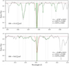 |
Fig. 2. Fit performed using the EWComputation module to the blended lines Fe I 6297.80 Å and Fe II 6516.08 Å, from the giant star HIP9313 taken with CHIRON. The right-most text contains the values of A, μ, and σ, the amplitude, mean, and standard deviation, respectively, of the best Gaussian fit, along with their corresponding uncertainties eA, eμ, and eσ. The grey lines are the absorption lines detected in the spectral range, and the green line the global fit to the data. The red region corresponds to the fit of the line, l, with its uncertainty, derived using the Gaussian parameters plus their uncertainties. The green block represents the equivalent width, quoted in the left-most text. The full procedure is explained in Appendix A. |
The uncertainty in the atmospheric parameters derived by SPECIES is estimated from the uncertainty in the correlation between the iron abundance and the excitation potential (for the temperature) and between the abundance and the reduced EW (for the microturbulent velocity); for the metallicity, it is the spread of abundances from the Fe I lines, and for the surface gravity, it is derived from the spread of the Fe I and Fe II lines (details can be found in SJ18).
The ATLAS9 model atmospheres assumes plane-parallel layers, as opposed to other models that assume a spherical geometry, such as the MARCS models (Gustafsson et al. 2008). In order to check that our selection of models does not affect the computation of parameters, we recomputed them using the MARCS models. We find that the differences between the atmospheric parameters are within their respective uncertainties and, therefore, the assumption of a plane-parallel atmosphere does not have a significant effect on the EXPRESS sample of stars.
3.1. Initial parameters
Before beginning the process of estimating the atmospheric parameters, we gathered photometric and astrometric information for each target. Parallax and proper motion were obtained from Gaia DR2 (Gaia Collaboration 2018) or the HIPPARCOS mission (van Leeuwen 2007), 2MASS JHK magnitudes from Cutri et al. (2003), Tycho-2 (BV)t magnitudes from Høg et al. (2000), Strömgren b − y, m1, and c1 from Hauck & Mermilliod (1998) or Holmberg et al. (2009), and Johnson BV(RI)c magnitudes from Koen et al. (2010), Casagrande et al. (2006), Beers et al. (2007), or Ducati (2002). We also corrected the magnitudes for dust extinction using the maps provided in Bovy et al. (2016), via the mwdust4 python package. In the case of the GaiaG magnitude, which is not included within the bandpasses of mwdust, we used AG = 2.35 E(B − V), from Bovy et al. (2014, 2016). We preferred to compute our own extinction rather than using the AG values provided in Gaia DR2 because we find that these are overestimated for the stars in our sample (average value of ∼0.2, when available), which are all nearby stars (average parallax ∼11 mas), away from the galactic centre, and are therefore expected to experience low dust extinction in average. Finally, if the parallaxes were obtained from Gaia DR2, we applied the systematic correction from Stassun & Torres (2018)5.
We used the parallax, along with the proper motion, to estimate the evolutionary state of each target following the classification scheme presented in Collier Cameron et al. (2007), which uses the photometric colour, J − H, and the reduced proper motion (RPM), defined as J + 5log(μ), with J as the apparent magnitude in the J-band and μ the proper motion. If the star is classified as a giant, we estimated its temperature following the relations from Alonso et al. (1999). In Sect. 4, we show how efficient that classification scheme was with regard to our sample and how the initial temperatures compare to the final values obtained from SPECIES.
Surface gravity was inferred as the minimum value between 3.5 and Eq. (1) from SJ18. Finally, for all the stars in the giant sample, the metallicity was set to an initial value of zero.
3.2. Physical parameters
The physical parameters, namely mass, radius, age, luminosity, and evolutionary stage, were estimated using the latest version of the isochrones6 package (Morton 2015). This package creates a model of the star based on the atmospheric parameters and estimates its physical parameters by interpolating through a grid of MESA Isochrones and Stellar Tracks (MIST, Dotter 2016) using MultiNest (Feroz et al. 2009; Buchner et al. 2014). The final values for each parameter will be drawn from the obtained distributions. The newest version of this package incorporates the interpolation of the isochrone grids using the equivalent evolutionary points (EEPs), which indicates the evolutionary stage of the star.
As described in Dotter (2016), EEPs are points in stellar evolution that can be identified in different evolutionary tracks and are created to allow for the interpolation between tracks defined for different initial stellar masses. In the case of the MIST models, they are divided into primary EEPs, defined following a physical motivation and secondary EEPs, which provide a uniform spacing between the primary EEPs. The phases that are relevant for this work are:
– Terminal age main sequence (TAMS), defined as the point where the central H mass fraction is 10−2, after which the star begins the burning of H outside the core and enters the RGB phase.
– Tip of the RGB (RGBTip), which is the point at which the stellar luminosity reaches a maximum (or Teff reaches a minimum), but before sustained He burning in the core has started. For low-mass stars (M < 2.00 M⊙, Paxton et al. 2010), this point denotes the beginning of the helium flash, when He burning begins under degenerate conditions in the core.
– Zero age core helium burning (ZACHeB), where sustained core He burning begins, which we refer to here as the HB phase.
– Terminal age core helium burning (TACHeB), when the central He fraction is 10−4, which denotes the end of the core helium burning. Subsequent evolutionary stages include the burning of He outside the core and carbon burning for high-mass stars.
A more detailed description and processes involved in defining the EEPs can be found in Dotter (2016). The use of EEPs in isochrones allows for the correct interpolation in the isochrone grids for the evolved stellar phases7. As Dotter (2016) pointed out, inaccuracy in the interpolation happens because of the wide scale of changes the star goes through after the main sequence, all at very short timescales, compared to the time spent in the main sequence. During the post-main sequence phases, tracks for very similar initial masses will lie very close to each other but, for a certain age, will show stars in completely different evolutionary stages. A simple interpolation scheme that does not take into account the faster evolutionary phase after the MS might not be able to fully reproduce the morphology of the evolution track. This is one of the reasons for the discrepancy between the results presented here and those in J11. The numbers referred as EEPs in the rest of the text correspond to the secondary EEPs.
During the interpolation process, we adopted a prior mass distribution following a Salpeter initial mass function (IMF), with α = 2.35. Similarly, we adopted a prior metallicity distribution, based on the local disk, following Casagrande et al. (2011)8 For the stellar age we adopted a flat prior in logarithmic scale, with bounds given as (105 − 1010.15) yr. Finally, the EEP has an uniform probability distribution, with 353 as the lower bound for giant stars (otherwise 200, to ensure no pre-main sequence stages), and 1710 as the upper bound. The atmospheric parameters derived previously (Teff, log g, and [Fe/H]), along with the photometric magnitudes and parallax (Sect. 3.1), were added to the likelihood function as  , where (xi, σi) correspond to the observed and computed properties and Ii is the model prediction for the i’th parameter (Montet et al. 2015).
One of the outputs from the physical parameter estimation is the EEP distribution for each star. Table 2 shows the correspondence between EEP and evolutionary phase. For the rest of the analysis in the paper, we consider 454 < EEP < 631 to be the RGB phase and 631 ≤ EEP ≤ 707 to be the HB phase. We also infer the probability of a star to be either in the RGB or the HB phase as pstate = ∑EEPstate/∑N, where N is the total EEP distribution size distribution.
Correspondance between equivalent evolutionary points (EEPs) and stellar evolutionary phase.
3.3. Rotational and macroturbulent velocity
We followed the method described in SJ18 to compute the rotational and macroturbulent velocities, which we summarise here. The macroturbulent velocity is computed following Eq. (1) in dos Santos et al. (2016) and for the cases where we obtain a very small or negative value, indicating that the temperature or surface gravity is outside of the range of applicability, we adopt Eq. (2) from Brewer et al. (2016). The rotational velocity was estimated by fitting rotationally broaden synthetic profiles to five different absorption lines. To obtain an estimate of the uncertainty in the rotational velocities, we first vary the normalised flux of each line by an amount, dy, with, dy, being drawn from a normal distribution with zero mean and width given by 1/S/N, with S/N as the signal-to-noise ratio of the spectrum. We then recompute the rotational velocity a total of 1000 iterations, obtaining a distribution of rotational velocities. The uncertainty is then taken as the standard deviation of the distribution. The final rotational velocity will correspond to the average of the velocities obtained for the five lines, with their corresponding errors. More details of the fitting procedure can be found in SJ18.
4. Results
The sample of giant stars from the EXPRESS project was first described and analysed in J11, using a broadly similar procedure to the one presented here for the estimation of atmospheric and physical parameters. Here, we improve on this analysis by using updated versions of the atmospheric models and the MOOG code, unavailable when J11 was published. We also estimate the equivalent widths using the method described in Appendix A, instead of using ARES (Sousa et al. 2007), as was done in J11. Additionally, here we use an updated version of the line list. We removed 68 lines from the original list used in J11, 54 Fe I and 14 Fe II lines, due to the consistently large uncertainties in the measured equivalent widths (σEW/EW > 0.5). The updated line list is given in Table B.1. In addition, here, we used higher quality spectra to measure the EWs, in terms of resolving power and S/N. For ∼30 stars presented in J11, we used FECH low S/N spectra at a resolution lower than FEROS and HARPS. As a consequence, the EWs and thus the derived atmospheric and physical parameters are largely uncertain. As an example, we highlight the case of the planet-host star HIP 105854, for which we used a low quality FECH spectrum for the analysis. In J11 the obtained mass was 2.1 ± 0.1 M⊙, a substantial overestimate of the mass obtained here (0.97 M⊙). This particular case was also noted by Campante et al. (2019), who used asteroseismology to derive a mass of 1.00 ± 0.16 M⊙, if the star is in HB, as obtained here (pHB = 0.88; see Table B.4). Finally, in the case of the physical parameters (such as mass and radius), we use the Gaia DR2 parallaxes, newer extinction maps, and we also employ a different set of evolutionary models for the purposes of this study.
The HR diagram for the EXPRESS stars is shown in Fig. 3. A sample of the catalogue produced by SPECIES, with a subset of columns, is shown in Table B.4. We also include in Table 3 the average values obtained for a set of Sun spectra, taken using a range of methods and instruments. The individual results are listed in Table B.5.
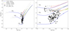 |
Fig. 3. H-R diagram of the giant star sample. The right panel is a close-up of the area where the stars in the sample are located. Open circles represent RGB stars and filled circles are HB stars. The tracks plotted have [Fe/H] = 0.0 and the different colours represent different phases in the stellar evolution. Grey lines represent the stages before the main sequence evolution (up to the TAMS, Table 2), and right after the end of core helium burning (TACHeB). For the meaning of the abbreviations and EEP number, see Table 2. |
Values obtained for the Sun spectra using SPECIES.
4.1. Comparison with the literature
We first analysed the stars from EXPRESS with results from interferometry and asteroseismology, which we used as a benchmark for the results obtained using our techniques. To this comparison, we also added a few other stars whose spectra are available from FEROS and HARPS, but are not necessary evolved stars. The list of stars with the results from SPECIES (for interferometry and asteroseismology) are listed in Table B.2 and the values from the literature are given in Table B.3. We then compared our results with other spectroscopic studies.
4.1.1. Interferometry
Precise stellar angular sizes can be obtained through long baseline interferometry, which can then be combined with parallax data and broadband photometry to estimate the size of a star. We compared a total of 12 targets (5 from the EXPRESS sample and 7 new targets with data from FEROS) with the radius from Gallenne et al. (2018), Tsantaki et al. (2013), and Rains et al. (2020) and the results are shown in Fig. 4 and Table 4. In the case of Tsantaki et al. (2013), the authors did not explicitly list the radius found through interferometry but, rather, showed the limb-darkened angular diameter θLD used, taken from the literature (the corresponding references are found in Tsantaki et al. 2013). We combined θLD with parallax information from either Gaia or HIPPARCOS (whichever was the most precise) to obtain the stellar radius.
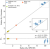 |
Fig. 4. Top panel: comparison between the radius measurement from SPECIES and from works using interferometry for the stars in our test sample. The black dotted line is the 1:1 relation. The inset correspond to a zoom of the squared regions. Bottom panel: difference SPECIES-literature. Uncertainties are computed considering both SPECIES and literature values ( |
Offsets between the radius from SPECIES, and from interferometry studies.
Overall, for the interferometry, we find a difference in the radius between SPECIES and the literature of Δ RINTER = −0.11 ± 0.29 R⊙, which is below the 2% level from the mean radius values. Here, the values are quoted as μ ± σ, the mean and standard deviation of the residual distribution, respectively. The comparison with interferometry is shown in Fig. 4. We find that the differences in radius are within a standard deviation of the individual values (Table 4), where our results are 0.54 R⊙ (∼5%) smaller Gallenne et al. (2018). These substantial differences are not seen when comparing with Tsantaki et al. (2013) and Rains et al. (2020), but those targets correspond to main sequence stars, whereas the targets from Gallenne et al. (2018) are giant stars. The source of our discrepancy with Gallenne et al. (2018) is not yet clear, but could be related to the calibration or limb-darkening model used for the estimation of the angular sizes.
4.1.2. Asteroseismology
The asteroseismology technique consists of looking at stellar oscillation spectra from either spectroscopy or photometry and then measuring two global oscillation quantities: the average frequency separation (Δν), and the frequency corresponding to the maximum oscillation power (νmax). In the case of solar-like oscillations, these values can then be used to estimate the stellar density and surface gravity by using scaling relations (Ulrich 1986; Brown et al. 1991; Kjeldsen & Bedding 1995) and by combining both quantities, it is possible to obtain the stellar mass and radius in a nearly model-independent approach. Another method widely used in the literature to obtain the stellar parameters is by using grid-based modelling techniques, which take as an input the individual frequency determinations or the global asteroseismic parameters, along with the effective temperature and metallicity, as well as other observational constraints. The scaling relations can also be included in the grid-based modelling. Even though this method is not model-independent, it has been found that the results given by the use of different pipelines, each using different stellar evolution models, are all in good agreement (Pinsonneault et al. 2018; Silva Aguirre et al. 2015). When the analysis is made using the grid-modelling approach, it is possible to also determine the stellar age. Age is a difficult parameter to fit for Soderblom (2010), but thus far, asteroseismology has been the most precise method for its estimation, with uncertainties on the order of ∼25% (Silva Aguirre & Serenelli 2016). The other properties derived from asteroseismology (such as mass and radius) have been shown to be accurate to the ∼10% level (Pinsonneault et al. 2018). A more detailed discussion on the subject of asteroseismology and the different pipelines available for the parameter estimation can be found in Chaplin & Miglio (2013), Silva Aguirre et al. (2020), and references therein.
We compared our estimates for the mass, radius, log g, and age for 15 targets (9 from EXPRESS and 6 new targets with data taken with FEROS) with values computed using asteroseismology from Morel et al. (2014), Campante et al. (2019), Jiang et al. (2020), Aguirre et al. (2020), and North et al. (2017). In Morel et al. (2014), the surface gravity is computed from the scaling relation that uses νmax and the stellar effective temperature. The temperature is computed from high-resolution spectroscopy, following the same method as in this work. As the authors do not list the values for Δν and νmax, it was not possible for us to separate the stellar mass and radius from the surface gravity. In Campante et al. (2019), Jiang et al. (2020), Aguirre et al. (2020), and North et al. (2017), the authors used temperature and metallicity values from the literature, which were used, together with the global asteroseismic parameters and astrometry information from Gaia (HIPPARCOS in the case of North et al. 2017), to retrieve the stellar parameters using grid-based modelling techniques. For Aguirre et al. (2020) and North et al. (2017), the log g values used for the comparison were estimated from their mass and radius results.
Figure 5 shows the comparison between SPECIES and the asteroseismic literature, and Table 5 lists the average differences. We find Δ log gASTERO = 0.07 ± 0.10 cgs, ΔRASTERO = −0.12 ± 0.26 R⊙, ΔMASTERO = 0.08 ± 0.12 M⊙, and ΔAgeASTERO = −0.55 ± 2.14 Gyr. These offsets show agreement at the 2.4% level for the surface gravity, 1.5% for the radius, 6.2% for the mass, and 11.9% for the age. The standard deviations are within the 5% level for the surface gravity and the radius, within the 10% for the mass, and just within the 47% level for the age. We also highlight that the average offset with the radius agrees with the one from interferometry. For all the parameters, we are within one standard deviation of the SPECIES-literature residual distributions, which leads us to conclude that our results agree with the asteroseismology ones.
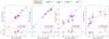 |
Fig. 5. Top panels: comparison between SPECIES and the asteroseismology studies for the stars in our test sample. The black dotted line in each panel is the 1:1 relation. Bottom panels: difference SPECIES-literature, same as in Fig. 4. The quoted text are the mean and standard deviation of the residuals for each quantity, and their percentage from the mean values. Surface gravity values were not given in Aguirre et al. (2020) and North et al. (2017), but were computed from their masses and radius. |
As we mentioned in the introduction, it is especially important to check the mass measurements of giant stars, computed using stellar evolution grids, with the results from other methods. We find that our mass estimates, as a whole, agree with the asteroseismic values within the uncertainties (with the exception of HIP4293, from Aguirre et al. 2020). This result validates the mass estimates with SPECIES, which are shown for the whole EXPRESS sample in the next section.
4.1.3. Spectroscopy
We compared our results for the EXPRESS sample with works in the literature that have adopted spectroscopy to derive the stellar parameters, namely: Jones et al. (2011), Jofré et al. (2015), Luck & Heiter (2007), Alves et al. (2015), Wittenmyer et al. (2016c), and the SWEET-Cat9 catalogue (Santos et al. 2013), which is a compilation of stellar parameters for stars with planets discovered in the literature. In the case of Luck & Heiter (2007), we compared with the parameters derived using spectroscopy and from Alves et al. (2015), we used the results from the Tsantaki et al. (2013) line list, as these have also been adopted by the authors. Figure 6 shows the comparison with our results and the mentioned works for six of the parameters computed by SPECIES.
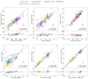 |
Fig. 6. Comparison between SPECIES and the literature for the EXPRESS stars. Bottom panels: difference SPECIES-Literature. The errorbar shows the average uncertainties in the points. The quoted text are the mean and standard deviation of the residuals for each quantity, and their percentage from the mean values. |
Offsets between the results from SPECIES, and from asteroseismic studies.
All these works from the literature use the same method for the derivation of the atmospheric parameters as in this paper and differences arise in the source of the data (different instruments and S/N), the measurement of the equivalent widths, the model atmospheres, and the iron line list used. In the case of the physical parameters, when available, they were estimated using different stellar evolution models. The average differences, with their uncertainties, and dispersion in the residuals (SPECIES – Literature) are listed in Table 6.
Residuals between our results and the literature.
As for the temperature, we find that our results are in general larger than the literature (ΔTeff = 22 ± 68 K), but the difference is within a single standard deviation of the data. In the case of the surface gravity and metallicity, our estimates are smaller than the literature, but both are within 1σ from zero, and represent less than 5% of the average log g and metallicity values for our sample. For the mass, our results are smaller than the literature (ΔM = −0.15 ± 0.31 M⊙), which is mostly driven by the comparison with J11, which we would comment more on the next paragraph. The difference of −0.25 M⊙ with respect to SWEET-Cat is driven mostly by four stars, two of which have large uncertainties (σ ≥ 0.45 M⊙), and if we remove those two objects the difference is reduced to −0.11 M⊙. Finally, for both the radius and luminosity we find that our results agree with the literature values at the 2% level.
As we mentioned earlier in this paper, there has been some debate in the literature as to whether the masses of giant stars are overestimated when using stellar evolution codes, partly due to the challenge that is posed by the process of interpolating through the post-main sequence tracks. This can be seen in our comparison with J11. We find an overall mass difference of ΔMJ11 = −0.28 ± 0.27 M⊙, with some targets being over 1 M⊙ smaller than in J11. This mass difference could be linked to an observation we mentioned in the introduction, namely, that stellar evolution tracks are degenerate for giant stars. This means that tracks corresponding to different masses occupy the same region in the HR diagram. Although incorporating precise values for the temperature, surface gravity, and metallicity to the interpolation helps to achieve a more accurate mass determination (Sousa et al. 2015), this might not be enough. As we mentioned in Sect. 3.2, the sampling of the evolution tracks in terms of the evolutionary state (the EEP in our case) helps in dealing with some of the complexity, as it takes into account, for example, how brief the post main sequence evolution is as compared to the total stellar lifetime (Girardi et al. 2013; Dotter 2016).
4.2. Comparison between log g and log gtri
Previous works have shown a systematic difference between the surface gravity derived from the ionization balance of iron lines (spectroscopic log g) and from the interpolation in a grid of evolutionary models, usually called a trigonometric log g (e.g., Gratton et al. 1996; Sestito et al. 2006; Jones et al. 2011; Jofré et al. 2014; Tsantaki et al. 2019; Slumstrup et al. 2019). Some of the proposed explanations for this disagreement are the line list used to compute the Fe II abundance, or problems with the fitting of the individual absorption lines, such as line blending or an incorrect placement of the continuum (Jones et al. 2011; Tsantaki et al. 2019), among others. Here, we also compared our derived spectroscopic and trigonometric log gs. Figure 7 shows our comparison between these two independent values. As can be seen in the figure, we find a good agreement between them, with an average difference of only 0.001 cgs, well below the individual mean 1-σ uncertainty. We find a few exceptions, for which |log g − log gtri|> 0.22 cgs. This value was derived in SJ18 after studying the difference in both quantities. For those stars, log gtri was adopted and the stellar parameters were recomputed, following SJ18. We found that by imposing log gtri as the final log g value, the rest of the parameters (Teff, [Fe/H] and the other physical parameters) were barely affected, with changes that are within their respective uncertainties.
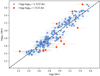 |
Fig. 7. Comparison between log g and log gtri. The black dashed line represents the 1:1 relation. |
4.3. Efficacy of the initial parameters
As noted in Sect. 3.1, we used the scheme from Collier Cameron et al. (2007) to classify the stars processed with SPECIES as dwarf or giant stars. Figure 8 replicates Fig. 8 from Collier Cameron et al. (2007), but using the EXPRESS sample. We find that following this scheme, 93% of stars were correctly classified as giant.
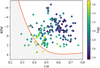 |
Fig. 8. Giant star classification, using the prescription from Collier Cameron et al. (2007), described in Sect. 3.1. The red line is the boundary between the dwarf and giant stars region. Points falling in the grey area are classified as dwarf stars. |
The initial temperature was derived from photometric information for each star, using the relations from Alonso et al. (1999). Even though photometric relations are available for 12 colours within the paper, we only used the ones corresponding to V − K, J − H, and J − K. That is because we had very few stars with precise magnitude measurements in the remaining bands and, therefore, we could not test the reliability of the temperature relations for those colours. As is shown in Alonso et al. (1999), the temperature relations also depend on the stellar metallicity. In the case of the initial parameters, we would have to use a photometric estimate of the metallicity. Most of the relations found in the literature use the Strömgren photometric system, but only a small number of stars in our sample had those magnitudes available. Therefore, we decided to set the initial metallicity to zero for all the stars in the sample.
The individual temperatures using the relations from Alonso et al. (1999), referred to as Teff, colour, for [Fe/H] = 0, compared to the final values from SPECIES, are shown in Fig. 9. We find that in all three cases, it is possible to relate both values through a linear fit of the form:
 (1)
(1)
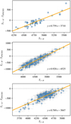 |
Fig. 9. Comparison between temperature computed with the photometric relations from Alonso et al. (1999) and SPECIES. Orange line represents the linear fit to the data, quoted in the text. |
with a and b listed in Table 7. The final temperature from photometry, referred as Teff, photo, is taken as the average weight of the individual colour temperatures, with the weights given by the uncertainty in the temperature estimates, computed from the uncertainties in the magnitude measurements, and the intrinsic uncertainties from the colour temperature relations, given in Alonso et al. (1999). In Fig. 10, we show the histogram of the difference between the values from SPECIES with the final temperature average from photometry. In the case where no correction is applied to the individual colour relations, we find an offset of 358 K with respect to the SPECIES values, whereas if the correction is applied, that offset is reduced to 9 K.
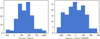 |
Fig. 10. Histogram of the difference between the temperature from SPECIES and from photometry, before (left panel) and after correcting (right panel) via the linear fits. |
Linear fit parameters between the temperature obtained using the colour relations from Alonso et al. (1999) and SPECIES, with Teff, colour − Teff, SPECIES = a Teff, colour + b.
We studied the effect of imposing [Fe/H] = 0 in the computation of Teff, photo by repeating the same analysis as before, but for two cases: setting [Fe/H] equal to the mean value found by SPECIES for the whole sample, −0.03 dex (Table 8), and using the metallicity computed by SPECIES for each individual star. We find that the parameters a and b from Eq. (1) do not change considerably, and that the mean difference between Teff, SPECIES − Teff, photo changes at most by 5 K compared to the values from setting [Fe/H] = 0. We conclude that for the stars in this sample, the assumption of [Fe/H]ini = 0 does not affect the value for Tini from photometry.
Mean and standard deviation for the parameters derived with SPECIES and how they change with the evolutionary stage.
4.4. Correlation between parameters
We studied the degree of correlation between the parameters derived by SPECIES. We estimated the Pearson correlation coefficients, r, between each parameter (Table B.6), and we consider the cases of clear correlation as the ones with |r|> 0.5. Figure 11 shows a selection of these strong correlations. Correlations for all the parameters are shown in Fig. B.1, generated using the corner10 module. After fitting polynomial functions to the data, we derived Eqs. (2)–(8).
 (2)
(2)
 (3)
(3)
 (4)
(4)
 (5)
(5)
 (6)
(6)
 (7)
(7)
 (8)
(8)
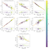 |
Fig. 11. Correlations found between parameters derived in this work. The orange lines are the polynomial fits. Bottom panels are the residuals after subtracting the polynomial fits. The colour scale represents the median EEP for each target. Titles show the scatter in the residuals for the total sample (σT), stars in the RGB (σRGB) and in the HB (σHB). |
where Θ = 5040/Teff.
The relation between the surface gravity and radius is expected by the physical definition of the surface gravity: g = GM/R2, where G is the gravitational constant, which can be rewritten as log g ∼ a(M)−b log R, with a(M) a value that depends on the mass. The mass range covered by the EXPRESS sample is for the most part very narrow (78% of the stars have 0.85 M⊙ ≤ M ≤ 2 M⊙), which allows us to approximate a(M) into a constant.
The relationship between microturbulence and surface gravity had been spotted before (Monaco et al. 2005; Kirby et al. 2009; Jones et al. 2011; Adibekyan et al. 2015; Mucciarelli & Bonifacio 2020) and takes the same shape as it does here (ξt = a + b log g). The coefficients we found (a = 2.95, b = −0.57) agree with those found in Jones et al. (2011).
The age-mass relation is related to the fact that once a star reaches the red giant phase, its age can be determined by the amount of time it spent in the main sequence (Casagrande et al. 2016). The time in the main sequence is directly related to the mass of the star, following tMS ∝ M−2.5. In our case, we find the power-law coefficient to be −3.0.
The luminosity is directly related to radius by its definition:  . As the range of temperatures mapped by the stars of the EXPRESS sample is narrow (σTeff = 128 K), we can set the temperature dependence as a constant, which leads us to Eq. (5).
We derive Eqs. (6) and (7) that relate the macroturbulent velocity, the radius, and the rotational velocity. We see that the macroturbulent velocity saturates out at for the faster rotating stars since the line profile is dominated by rotation in these cases, no matter the stellar spectral type. The macroturbulence is driven by the stellar convective flows and, hence, temperature, whereas the rotation velocity is tied to the evolution and, hence, given the range of temperatures that we are sensitive to, we can expect the rotation velocity to span a much wider range than the macroturbulent velocity.
Finally, Eq. (8) tells us that more massive stars also have larger surface temperatures, although the effect is more clear for core-helium burning stars given that their position in the HB is determined by their mass (with more massive stars to the left of the HB).
From Table B.6, we can also see a large correlation coefficient between the stellar mass and luminosity. Both quantities are plotted in Fig. 12. For stars with M < 2 M⊙, the luminosity during the RGB will depend on the core mass, which explains the large spread seen in the diagram. During the HB, the luminosity of the star will be directly proportional to the helium core mass. After the helium flash, all stars will begin the HB with the same core mass, which explains why all HB stars have an almost constant luminosity, independent of mass. Stars with M > 2 M⊙ do not form a degenerate helium core, instead igniting helium quietly, which explains their different behaviour from lower-mass stars. The strong correlation seen in Table B.6 for mass and luminosity is driven mostly by the population with M > 2 M⊙, but these correspond to only 33 stars; therefore, we can not confidently perform a regression fit.
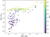 |
Fig. 12. Mass-luminosity diagram for the EXPRESS sample. The colour scale represents the median EEP for each target. |
The rest of the relations with large correlation coefficients (Table B.6) can be inferred from the relations we have already presented (Eqs. (2)–(8)). For example, vmac is correlated with both stellar radius and luminosity, and luminosity and radius are correlated with each other as well; therefore, it is possible to infer the relation between vmac and L⋆ from Eqs. (5) and (6).
4.5. Evolutionary stage
As mentioned in Sect. 3.2, one of the outputs from isochrones is the EEP state for each star. We consider the final EEP value for a certain star to be the median of the EEP distribution and follow the RGB and HB definition from Sect. 3.2. Figure 13 shows the distribution of EEP values for our sample. We find that 61% of stars (101) are in the RGB phase, while the other 39% (65) are in the HB.
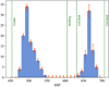 |
Fig. 13. Distribution of the stellar evolutionary stage for the EXPRESS sample. The errorbars in each bin reflect the uncertainty in the EEP values, given by the 16% and 84% percentiles of the EEP distribution for each star. |
Figure 14 shows the distribution of the stellar parameters as a function of evolutionary stage, with mean values separated into total, RGB, and HB distributions, listed in Table 8. We find that there is no difference in the temperature and metallicity distributions between RGB and HB stars. We also find that the EXPRESS sample is slightly metal poor (![Mathematical equation: $ \overline{\mathrm{[Fe/H]}} $](/articles/aa/full_html/2021/03/aa39357-20/aa39357-20-eq13.gif) = −0.03 dex), which is similar to what has been seen in other radial velocity searches around evolved stars (Döllinger et al. 2009; Mortier et al. 2013).
= −0.03 dex), which is similar to what has been seen in other radial velocity searches around evolved stars (Döllinger et al. 2009; Mortier et al. 2013).
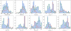 |
Fig. 14. Distribution of some of the parameters derived by SPECIES, separated by their evolutionary stage. The red line corresponds to the HB distribution and the green line to the RGB distribution. The blue histogram represents the total of both distributions. |
When looking at the size distribution, HB stars dominate the distribution for R > 9 R⊙ and, in turn, they have, on average, larger radii than RGB stars. They are also distributed around 8.3 < R/R⊙ < 16.5, whereas, RGB stars can cover a larger range, with 2.4 < R/R⊙ < 15. This radius difference between RGB and HB stars is reflected in the distribution of luminosity, surface gravity, and micro and macroturbulence velocity because of the correlations found in Sect. 4.4. We find that HB stars are more luminous and they have, on average, smaller log g and larger micro and macro turbulent velocity than RGB stars.
Low-mass stars (M < 2 M⊙) are mostly found in the RGB phase (69%), which is explained by the fact that the evolutionary timescale of this phase is longer for these stars than more massive stars and, therefore, is more probable to find them at that stage. The near lack of RGB stars with masses, M > 2 M⊙, is explained by the fact that intermediate mass stars do not go through the helium flash (the ignition of helium burning in the stellar core from degenerate conditions) and, thus, the lifetime of the RGB phase is much shorter than for lower-mass stars (Girardi et al. 2013). HB stars also cover a large range of possible masses (from 0.9 M⊙ to 3.06 M⊙), but RGB stars are mostly clustered around 1.4 M⊙. The dispersion of the residuals from the correlations adjusted in the previous section are large for HB stars in the case of the radius with log g. That could be explained by our approximation of the mass dependency on Eq. (2) to a constant, which is better fitted for RGB stars with a narrow range of masses than for HB stars. Finally, we find that HB stars have, on average, larger rotational velocities than RGB stars.
5. Summary and conclusions
In this work, we present a number of atmospheric and physical parameters of the EXPRESS programme sample, derived using the SPECIES code. We have introduced some improvements to SPECIES, including an updated version of the line list, a new routine to measure EWs of the iron lines, and the addition of the EEP into the interpolation of evolutionary models. Similarly, here we use higher quality stellar spectra, more accurate parallaxes from the Gaia DR2, and newer extinction maps, as compared to the original catalogue. Based on the posterior probabilities, we find that 101 stars are most probably in the RGB and 65 are probably in the HB. The separation of both stages is important not only for breaking the degeneracy in the H-R diagram and the correct estimation of the stellar mass, but also for the study of the effect of stellar evolution in planetary systems.
We compare our results with the relevant asteroseismology studies. Overall, we find an agreement at the 2% level in the stellar radii and at the 6% level in the stellar mass. By comparing our stellar radii with interferometric studies, we also find an agreement better than 2%. These results validate our method and show the robustness of SPECIES for accurately deriving stellar parameters.
Similarly, we compared our temperature, surface gravity, metallicity, mass, radius, and stellar luminosity with estimates from other spectroscopic catalogues. We find a good agreement for all the parameters, with mean differences within 2%. The only exception is the mass, for which we find an overall difference of −0.15 M⊙, corresponding to ∼9% difference. The largest differences are with respect to J11. This could be due to the differences in the line list, the stellar evolution models and interpolation procedure, the quality of the spectra used, or to the complexity of estimating stellar masses for giant stars using stellar evolution tracks, as these are degenerate in the parameter space giant stars occupy.
In addition, we studied the correlations between the parameters and find six relations, most of them driven by physical processes (log g-radius, age-mass, and luminosity-radius) and others already detected in previous works (microturbulence-log g). We also detect relations between the macroturbulence velocity and the radius, and between the macroturbulence and rotational velocity.
Finally we compared our spectroscopic and photometric log gs to investigate for any potential systematic difference, as this has been widely reported in the literature. We find an excellent agreement between these two quantities, with a mean difference of 0.001 cgs. This result further demonstrates the internal consistency and robustness of the method.
In the sample presented in J11 there were two missing stars.
February 2017 version.
Recently, Chan & Bovy (2020) computed an updated zero-point parallax correction, but the value is within the uncertainties of the parallaxes for the stars in this study, therefore we decided to keep the correction from Stassun & Torres (2018) as it would not greatly affect our results.
For a given metallicity value x, the probability density function takes the form P(x) = w0(w1N1(x)+w2N2(x)), where Ni = G(μi, σi) represents a Gaussian distribution with parameters (μi, σi), and the wi terms are normalisation factors.
Also available on its own at https://github.com/msotov/EWComputation
IRAF is distributed by the National Optical Astronomy Observatories, which are operated by the Association of Universities for Research in Astronomy, Inc., under a cooperative agreement with the National Science Foundation.
Acknowledgments
MGS acknowledges support from STFC through the Consolidated Grant ST/M001202/1. JSJ acknowledges support by FONDECYT grant 1201371 and partial support from CONICYT project Basal AFB-170002. This research has made use of the VizieR catalogue access tool, CDS, Strasbourg, France (DOI: https://doi.org/10.26093/cds/vizier). The original description of the VizieR service was published in Ochsenbein et al. (2000).
References
- Adibekyan, V. Z., Benamati, L., Santos, N. C., et al. 2015, MNRAS, 450, 1900 [NASA ADS] [CrossRef] [Google Scholar]
- Aguirre, V. S., Stello, D., Stokholm, A., et al. 2020, ApJ, 889, L34 [CrossRef] [Google Scholar]
- Alonso, A., Arribas, S., & Martínez-Roger, C. 1999, A&AS, 140, 261 [NASA ADS] [CrossRef] [EDP Sciences] [Google Scholar]
- Alves, S., Benamati, L., Santos, N. C., et al. 2015, MNRAS, 448, 2749 [NASA ADS] [CrossRef] [Google Scholar]
- Andreasen, D. T., Sousa, S. G., Tsantaki, M., et al. 2017, A&A, 600, A69 [NASA ADS] [CrossRef] [EDP Sciences] [Google Scholar]
- Aurière, M. 2003, in EAS Pub. Ser., eds. J. Arnaud, & N. Meunier, 9, 105 [CrossRef] [Google Scholar]
- Bedell, M., Bean, J. L., Meléndez, J., et al. 2017, ApJ, 839, 94 [NASA ADS] [CrossRef] [Google Scholar]
- Beers, T. C., Flynn, C., Rossi, S., et al. 2007, ApJS, 168, 128 [NASA ADS] [CrossRef] [Google Scholar]
- Blanco-Cuaresma, S., Soubiran, C., Jofré, P., & Heiter, U. 2014, A&A, 566, A98 [NASA ADS] [CrossRef] [EDP Sciences] [Google Scholar]
- Bluhm, P., Jones, M. I., Vanzi, L., et al. 2016, A&A, 593, A133 [NASA ADS] [CrossRef] [EDP Sciences] [Google Scholar]
- Boggs, P. T., & Rogers, J. E. 1990, Contemp. Math., 112, 183 [CrossRef] [Google Scholar]
- Borgniet, S., Lagrange, A. M., Meunier, N., et al. 2019, A&A, 621, A87 [NASA ADS] [CrossRef] [EDP Sciences] [Google Scholar]
- Bovy, J., Nidever, D. L., Rix, H.-W., et al. 2014, ApJ, 790, 127 [Google Scholar]
- Bovy, J., Rix, H.-W., Green, G. M., Schlafly, E. F., & Finkbeiner, D. P. 2016, ApJ, 818, 130 [NASA ADS] [CrossRef] [Google Scholar]
- Brahm, R., Jordán, A., & Espinoza, N. 2017, PASP, 129, 034002 [NASA ADS] [CrossRef] [Google Scholar]
- Brewer, J. M., Fischer, D. A., Valenti, J. A., & Piskunov, N. 2016, ApJS, 225, 32 [Google Scholar]
- Brown, T. M., Gilliland, R. L., Noyes, R. W., & Ramsey, L. W. 1991, ApJ, 368, 599 [NASA ADS] [CrossRef] [Google Scholar]
- Buchner, J., Georgakakis, A., Nandra, K., et al. 2014, A&A, 564, A125 [NASA ADS] [CrossRef] [EDP Sciences] [Google Scholar]
- Campante, T. L., Corsaro, E., Lund, M. N., et al. 2019, ApJ, 885, 31 [Google Scholar]
- Casagrande, L., Portinari, L., & Flynn, C. 2006, MNRAS, 373, 13 [NASA ADS] [CrossRef] [Google Scholar]
- Casagrande, L., Schönrich, R., Asplund, M., et al. 2011, A&A, 530, A138 [NASA ADS] [CrossRef] [EDP Sciences] [Google Scholar]
- Casagrande, L., Silva Aguirre, V., Schlesinger, K. J., et al. 2016, MNRAS, 455, 987 [NASA ADS] [CrossRef] [Google Scholar]
- Castelli, F., & Kurucz, R. L. 2004, ArXiv e-prints [arXiv:astro-ph/0405087] [Google Scholar]
- Chan, V. C., & Bovy, J. 2020, MNRAS, 493, 4367 [CrossRef] [Google Scholar]
- Chaplin, W. J., & Miglio, A. 2013, ARA&A, 51, 353 [Google Scholar]
- Collier Cameron, A., Wilson, D. M., West, R. G., et al. 2007, MNRAS, 380, 1230 [NASA ADS] [CrossRef] [Google Scholar]
- Currie, T. 2009, ApJ, 694, L171 [NASA ADS] [CrossRef] [Google Scholar]
- Cutri, R. M., Skrutskie, M. F., van Dyk, S., et al. 2003, 2MASS All Sky Catalog of Point Sources, http://irsa.ipac.caltech.edu/applications/Gator/ [Google Scholar]
- Dekker, H., D’Odorico, S., Kaufer, A., Delabre, B., & Kotzlowski, H. 2000, in Society of Photo-Optical Instrumentation Engineers (SPIE) Conference Series, eds. M. Iye, & A. F. Moorwood, Proc. SPIE, 4008, 534 [Google Scholar]
- Döllinger, M. P., Hatzes, A. P., Pasquini, L., Guenther, E. W., & Hartmann, M. 2009, A&A, 505, 1311 [NASA ADS] [CrossRef] [EDP Sciences] [Google Scholar]
- dos Santos, L. A., Meléndez, J., do Nascimento, J. D., et al. 2016, A&A, 592, A156 [NASA ADS] [CrossRef] [EDP Sciences] [Google Scholar]
- Dotter, A. 2016, ApJS, 222, 8 [NASA ADS] [CrossRef] [Google Scholar]
- Ducati, J. R. 2002, VizieR Online Data Catalog: II/237 [Google Scholar]
- Feroz, F., Hobson, M. P., & Bridges, M. 2009, MNRAS, 398, 1601 [NASA ADS] [CrossRef] [Google Scholar]
- Fischer, D. A., & Valenti, J. 2005, ApJ, 622, 1102 [Google Scholar]
- Fischer, D., Driscoll, P., Isaacson, H., et al. 2009, ApJ, 703, 1545 [NASA ADS] [CrossRef] [Google Scholar]
- Frink, S., Quirrenbach, A., Fischer, D., Röser, S., & Schilbach, E. 2001, PASP, 113, 173 [NASA ADS] [CrossRef] [Google Scholar]
- Gaia Collaboration (Brown, A. G. A., et al.) 2018, A&A, 616, A1 [NASA ADS] [CrossRef] [EDP Sciences] [Google Scholar]
- Galland, F., Lagrange, A. M., Udry, S., et al. 2005, A&A, 443, 337 [NASA ADS] [CrossRef] [EDP Sciences] [Google Scholar]
- Gallenne, A., Pietrzyński, G., Graczyk, D., et al. 2018, A&A, 616, A68 [NASA ADS] [CrossRef] [EDP Sciences] [Google Scholar]
- Ghezzi, L., Cunha, K., Schuler, S. C., & Smith, V. V. 2010, ApJ, 725, 721 [NASA ADS] [CrossRef] [Google Scholar]
- Ghezzi, L., Montet, B. T., & Johnson, J. A. 2018, ApJ, 860, 109 [NASA ADS] [CrossRef] [Google Scholar]
- Girardi, L., Marigo, P., Bressan, A., & Rosenfield, P. 2013, ApJ, 777, 142 [NASA ADS] [CrossRef] [Google Scholar]
- Gratton, R. G., Carretta, E., & Castelli, F. 1996, A&A, 314, 191 [NASA ADS] [Google Scholar]
- Gray, D. F. 2005, The Observation and Analysis of Stellar Photospheres (Cambridge: Cambridge University Press) [CrossRef] [Google Scholar]
- Gustafsson, B., Edvardsson, B., Eriksson, K., et al. 2008, A&A, 486, 951 [NASA ADS] [CrossRef] [EDP Sciences] [Google Scholar]
- Hatzes, A. P., Guenther, E. W., Endl, M., et al. 2005, A&A, 437, 743 [NASA ADS] [CrossRef] [EDP Sciences] [Google Scholar]
- Hauck, B., & Mermilliod, M. 1998, A&AS, 129, 431 [NASA ADS] [CrossRef] [EDP Sciences] [Google Scholar]
- Hekker, S., & Meléndez, J. 2007, A&A, 475, 1003 [NASA ADS] [CrossRef] [EDP Sciences] [Google Scholar]
- Hekker, S., Reffert, S., Quirrenbach, A., et al. 2006, A&A, 454, 943 [NASA ADS] [CrossRef] [EDP Sciences] [Google Scholar]
- Hinkle, K., & Wallace, L. 2005, in Cosmic Abundances as Records of Stellar Evolution and Nucleosynthesis, eds. I. Barnes, G. Thomas, & F. N. Bash, ASP Conf. Ser., 336, 321 [Google Scholar]
- Hinkle, K., Wallace, L., Valenti, J., & Harmer, D. 2000, Visible and Near Infrared Atlas of the Arcturus Spectrum 3727–9300 A (San Francisco: ASP) [Google Scholar]
- Høg, E., Fabricius, C., Makarov, V. V., et al. 2000, A&A, 355, L27 [Google Scholar]
- Holmberg, J., Nordström, B., & Andersen, J. 2009, A&A, 501, 941 [NASA ADS] [CrossRef] [EDP Sciences] [Google Scholar]
- Ida, S., & Lin, D. N. C. 2004, ApJ, 604, 388 [NASA ADS] [CrossRef] [PubMed] [Google Scholar]
- Jenkins, J. S., Jones, H. R. A., Pavlenko, Y., et al. 2008, A&A, 485, 571 [NASA ADS] [CrossRef] [EDP Sciences] [Google Scholar]
- Jenkins, J. S., Jones, H. R. A., Tuomi, M., et al. 2017, MNRAS, 466, 443 [NASA ADS] [CrossRef] [Google Scholar]
- Jiang, C., Bedding, T. R., Stassun, K. G., et al. 2020, ApJ, 896, 65 [Google Scholar]
- Jofré, P., Heiter, U., Soubiran, C., et al. 2014, A&A, 564, A133 [NASA ADS] [CrossRef] [EDP Sciences] [Google Scholar]
- Jofré, E., Petrucci, R., Saffe, C., et al. 2015, A&A, 574, A50 [NASA ADS] [CrossRef] [EDP Sciences] [Google Scholar]
- Johnson, J. A., Fischer, D. A., Marcy, G. W., et al. 2007, ApJ, 665, 785 [NASA ADS] [CrossRef] [Google Scholar]
- Johnson, J. A., Clanton, C., Howard, A. W., et al. 2011, ApJS, 197, 26 [NASA ADS] [CrossRef] [Google Scholar]
- Johnson, J. A., Morton, T. D., & Wright, J. T. 2013, ApJ, 763, 53 [NASA ADS] [CrossRef] [Google Scholar]
- Jones, M. I., Jenkins, J. S., Rojo, P., & Melo, C. H. F. 2011, A&A, 536, A71 [NASA ADS] [CrossRef] [EDP Sciences] [Google Scholar]
- Jones, M. I., Jenkins, J. S., Rojo, P., Melo, C. H. F., & Bluhm, P. 2013, A&A, 556, A78 [NASA ADS] [CrossRef] [EDP Sciences] [Google Scholar]
- Jones, M. I., Jenkins, J. S., Bluhm, P., Rojo, P., & Melo, C. H. F. 2014, A&A, 566, A113 [NASA ADS] [CrossRef] [EDP Sciences] [Google Scholar]
- Jones, M. I., Jenkins, J. S., Rojo, P., Melo, C. H. F., & Bluhm, P. 2015a, A&A, 573, A3 [NASA ADS] [CrossRef] [EDP Sciences] [Google Scholar]
- Jones, M. I., Jenkins, J. S., Rojo, P., Olivares, F., & Melo, C. H. F. 2015b, A&A, 580, A14 [NASA ADS] [CrossRef] [EDP Sciences] [Google Scholar]
- Jones, M. I., Jenkins, J. S., Brahm, R., et al. 2016, A&A, 590, A38 [NASA ADS] [CrossRef] [EDP Sciences] [Google Scholar]
- Jones, M. I., Brahm, R., Wittenmyer, R. A., et al. 2017, A&A, 602, A58 [NASA ADS] [CrossRef] [EDP Sciences] [Google Scholar]
- Jones, M. I., Wittenmyer, R., Aguilera-Gómez, C., et al. 2021, A&A, 646, A131 [EDP Sciences] [Google Scholar]
- Kaufer, A., Stahl, O., Tubbesing, S., et al. 1999, The Messenger, 95, 8 [Google Scholar]
- Kirby, E. N., Guhathakurta, P., Bolte, M., Sneden, C., & Geha, M. C. 2009, ApJ, 705, 328 [NASA ADS] [CrossRef] [Google Scholar]
- Kjeldsen, H., & Bedding, T. R. 1995, A&A, 293, 87 [NASA ADS] [Google Scholar]
- Koen, C., Kilkenny, D., van Wyk, F., & Marang, F. 2010, MNRAS, 403, 1949 [Google Scholar]
- Kunitomo, M., Ikoma, M., Sato, B., Katsuta, Y., & Ida, S. 2011, ApJ, 737, 66 [NASA ADS] [CrossRef] [Google Scholar]
- Lagrange, A. M., Desort, M., Galland, F., Udry, S., & Mayor, M. 2009, A&A, 495, 335 [NASA ADS] [CrossRef] [EDP Sciences] [Google Scholar]
- Lloyd, J. P. 2011, ApJ, 739, L49 [NASA ADS] [CrossRef] [Google Scholar]
- Lloyd, J. P. 2013, ApJ, 774, L2 [NASA ADS] [CrossRef] [Google Scholar]
- Luck, R. E., & Heiter, U. 2007, AJ, 133, 2464 [NASA ADS] [CrossRef] [Google Scholar]
- Maldonado, J., Villaver, E., & Eiroa, C. 2013, A&A, 554, A84 [NASA ADS] [CrossRef] [EDP Sciences] [Google Scholar]
- Monaco, L., Bellazzini, M., Bonifacio, P., et al. 2005, A&A, 441, 141 [NASA ADS] [CrossRef] [EDP Sciences] [MathSciNet] [Google Scholar]
- Montet, B. T., Morton, T. D., Foreman-Mackey, D., et al. 2015, ApJ, 809, 25 [NASA ADS] [CrossRef] [Google Scholar]
- Morel, T., Miglio, A., Lagarde, N., et al. 2014, A&A, 564, A119 [NASA ADS] [CrossRef] [EDP Sciences] [Google Scholar]
- Mortier, A., Santos, N. C., Sousa, S. G., et al. 2013, A&A, 557, A70 [NASA ADS] [CrossRef] [EDP Sciences] [Google Scholar]
- Morton, T. D. 2015, Astrophysics Source Code Library [record ascl:1503.010] [Google Scholar]
- Mucciarelli, A., & Bonifacio, P. 2020, A&A, 640, A87 [CrossRef] [EDP Sciences] [Google Scholar]
- Niedzielski, A., Konacki, M., Wolszczan, A., et al. 2007, ApJ, 669, 1354 [NASA ADS] [CrossRef] [Google Scholar]
- North, T. S. H., Campante, T. L., Miglio, A., et al. 2017, MNRAS, 472, 1866 [NASA ADS] [CrossRef] [Google Scholar]
- Ochsenbein, F., Bauer, P., & Marcout, J. 2000, A&AS, 143, 23 [NASA ADS] [CrossRef] [EDP Sciences] [Google Scholar]
- Pasquini, L., Döllinger, M. P., Weiss, A., et al. 2007, A&A, 473, 979 [NASA ADS] [CrossRef] [EDP Sciences] [Google Scholar]
- Paxton, B., Bildsten, L., Dotter, A., et al. 2010, ApJS, 192, 3 [Google Scholar]
- Perryman, M. A. C., Lindegren, L., Kovalevsky, J., et al. 1997, A&A, 500, 501 [NASA ADS] [Google Scholar]
- Pinsonneault, M. H., Elsworth, Y. P., Tayar, J., et al. 2018, ApJS, 239, 32 [Google Scholar]
- Rains, A. D., Ireland, M. J., White, T. R., Casagrande, L., & Karovicova, I. 2020, MNRAS, 493, 2377 [Google Scholar]
- Ramírez, I., & Allende Prieto, C. 2011, ApJ, 743, 135 [NASA ADS] [CrossRef] [Google Scholar]
- Reffert, S., Bergmann, C., Quirrenbach, A., Trifonov, T., & Künstler, A. 2015, A&A, 574, A116 [NASA ADS] [CrossRef] [EDP Sciences] [Google Scholar]
- Ribas, Á., Bouy, H., & Merín, B. 2015, A&A, 576, A52 [NASA ADS] [CrossRef] [EDP Sciences] [Google Scholar]
- Royer, F., Zorec, J., & Gómez, A. E. 2007, A&A, 463, 671 [NASA ADS] [CrossRef] [EDP Sciences] [Google Scholar]
- Santos, N. C., Israelian, G., Mayor, M., Rebolo, R., & Udry, S. 2003, A&A, 398, 363 [NASA ADS] [CrossRef] [EDP Sciences] [Google Scholar]
- Santos, N. C., Sousa, S. G., Mortier, A., et al. 2013, A&A, 556, A150 [NASA ADS] [CrossRef] [EDP Sciences] [Google Scholar]
- Sato, B., Kambe, E., Takeda, Y., et al. 2005, PASJ, 57, 97 [Google Scholar]
- Sato, B., Omiya, M., Harakawa, H., et al. 2012, PASJ, 64, 135 [NASA ADS] [CrossRef] [Google Scholar]
- Schlaufman, K. C., & Winn, J. N. 2013, ApJ, 772, 143 [NASA ADS] [CrossRef] [Google Scholar]
- Schrijver, C. J., & Pols, O. R. 1993, A&A, 278, 51 [Google Scholar]
- Serenelli, A., Weiss, A., Aerts, C., et al. 2020, A&ARv, submitted [arXiv:2006.10868] [Google Scholar]
- Sestito, P., Bragaglia, A., Randich, S., et al. 2006, A&A, 458, 121 [NASA ADS] [CrossRef] [EDP Sciences] [Google Scholar]
- Setiawan, J., Pasquini, L., da Silva, L., von der Lühe, O., & Hatzes, A. 2003, A&A, 397, 1151 [NASA ADS] [CrossRef] [EDP Sciences] [Google Scholar]
- Silva Aguirre, V., & Serenelli, A. M. 2016, Astron. Nachr., 337, 823 [NASA ADS] [CrossRef] [Google Scholar]
- Silva Aguirre, V., Davies, G. R., Basu, S., et al. 2015, MNRAS, 452, 2127 [NASA ADS] [CrossRef] [Google Scholar]
- Silva Aguirre, V., Christensen-Dalsgaard, J., Cassisi, S., et al. 2020, A&A, 635, A164 [NASA ADS] [CrossRef] [EDP Sciences] [Google Scholar]
- Slumstrup, D., Grundahl, F., Silva Aguirre, V., & Brogaard, K. 2019, A&A, 622, A111 [NASA ADS] [CrossRef] [EDP Sciences] [Google Scholar]
- Sneden, C. A. 1973, PhD Thesis, The University of Texas at Austin, USA [Google Scholar]
- Soderblom, D. R. 2010, ARA&A, 48, 581 [NASA ADS] [CrossRef] [Google Scholar]
- Soto, M. G., & Jenkins, J. S. 2018, A&A, 615, A76 [NASA ADS] [CrossRef] [EDP Sciences] [Google Scholar]
- Sousa, S. G., Santos, N. C., Israelian, G., Mayor, M., & Monteiro, M. J. P. F. G. 2007, A&A, 469, 783 [NASA ADS] [CrossRef] [EDP Sciences] [Google Scholar]
- Sousa, S. G., Santos, N. C., Mortier, A., et al. 2015, A&A, 576, A94 [NASA ADS] [CrossRef] [EDP Sciences] [Google Scholar]
- Sousa, S. G., Adibekyan, V., Delgado-Mena, E., et al. 2018, A&A, 620, A58 [NASA ADS] [CrossRef] [EDP Sciences] [Google Scholar]
- Stassun, K. G., & Torres, G. 2018, ApJ, 862, 61 [Google Scholar]
- Stock, S., Reffert, S., & Quirrenbach, A. 2018, A&A, 616, A33 [NASA ADS] [CrossRef] [EDP Sciences] [Google Scholar]
- Takeda, Y., & Tajitsu, A. 2015, MNRAS, 450, 397 [NASA ADS] [CrossRef] [Google Scholar]
- Tokovinin, A., Fischer, D. A., Bonati, M., et al. 2013, PASP, 125, 1336 [NASA ADS] [CrossRef] [Google Scholar]
- Trifonov, T., Reffert, S., Tan, X., Lee, M. H., & Quirrenbach, A. 2014, A&A, 568, A64 [NASA ADS] [CrossRef] [EDP Sciences] [Google Scholar]
- Tsantaki, M., Sousa, S. G., Adibekyan, V. Z., et al. 2013, A&A, 555, A150 [NASA ADS] [CrossRef] [EDP Sciences] [Google Scholar]
- Tsantaki, M., Santos, N. C., Sousa, S. G., et al. 2019, MNRAS, 485, 2772 [NASA ADS] [CrossRef] [Google Scholar]
- Ulrich, R. K. 1986, ApJ, 306, L37 [Google Scholar]
- Valenti, J. A., & Fischer, D. A. 2005, ApJS, 159, 141 [NASA ADS] [CrossRef] [MathSciNet] [Google Scholar]
- van Leeuwen, F. 2007, A&A, 474, 653 [NASA ADS] [CrossRef] [EDP Sciences] [Google Scholar]
- Vanzi, L., Zapata, A., Flores, M., et al. 2018, MNRAS, 477, 5041 [NASA ADS] [CrossRef] [Google Scholar]
- Villaver, E., & Livio, M. 2009, ApJ, 705, L81 [NASA ADS] [CrossRef] [Google Scholar]
- Villaver, E., Livio, M., Mustill, A. J., & Siess, L. 2014, ApJ, 794, 3 [NASA ADS] [CrossRef] [Google Scholar]
- Vogt, S. S., Allen, S. L., Bigelow, B. C., et al. 1994, in Instrumentation in Astronomy VIII, eds. D. L. Crawford, & E. R. Craine, SPIE Conf. Ser., 2198, 362 [NASA ADS] [CrossRef] [Google Scholar]
- Wittenmyer, R. A., Endl, M., Wang, L., et al. 2011, ApJ, 743, 184 [NASA ADS] [CrossRef] [Google Scholar]
- Wittenmyer, R. A., Butler, R. P., Wang, L., et al. 2016a, MNRAS, 455, 1398 [NASA ADS] [CrossRef] [Google Scholar]
- Wittenmyer, R. A., Johnson, J. A., Butler, R. P., et al. 2016b, ApJ, 818, 35 [NASA ADS] [CrossRef] [Google Scholar]
- Wittenmyer, R. A., Liu, F., Wang, L., et al. 2016c, AJ, 152, 19 [NASA ADS] [CrossRef] [Google Scholar]
- Wittenmyer, R. A., Jones, M. I., Zhao, J., et al. 2017, AJ, 153, 51 [NASA ADS] [CrossRef] [Google Scholar]
Appendix A: Equivalent width computation
The equivalent widths (EWs) were computed using the EWComputation module inside SPECIES11. For each line at wavelength l in a given linelist, this module: (1) selects a region within 3 Å from the line and normalises the spectrum; (2) detects the absorption lines within the region; (3) fits a Gaussian-like profile to the line; and (4) computes the equivalent width of the line based on the fit parameters, and its corresponding uncertainty. Steps (1) and (2) were written following the prescription from Sousa et al. (2007).
A.1. Continuum normalization
The continuum normalization is done by fitting second-degree polynomials to the data and rejecting the points that lie further than rejt from the polynomial. The value rejt was first introduced in Sousa et al. (2007) and is defined in SPECIES as rejt = 1−1/S/N, where S/N is the signal-to-noise ratio of the line region. The S/N is typically taken from the headers of the spectra and it can be a global value, representing the whole spectrum, or have different values depending on the wavelength of the data.
A.2. Line detection
The detection of spectral lines is done by identifying the regions in the spectrum where the derivative is zero and where the second-degree derivative is positive, indicating that the point corresponds to a local minimum. Before doing the derivations, the spectrum is smoothed by taking the convolution with a Box Kernel of size 4 and only the points with flux < −0.02 are considered as spectral lines. This is done when dealing with very noisy data, where fluctuations in the continuum can be mistaken as line profiles. This will result in a set of N lines centred at wavelengths μi, where i = 1, …, N. We additionally define the index I which refers to the line closest to the target point, as defined by the criterion μI = MIN{|μi − l|}.
A.3. Line profile fit
Once the N absorption lines are identified, we assume that each line follows a Gaussian-shaped profile, centered at wavelengths μi. The spectrum S at wavelength w can then be written as:
![Mathematical equation: $$ \begin{aligned} S({ w}) = \sum _{i=1}^N\,A_i \exp {\left[-({ w}-\mu _i)^2/2\sigma _i^2\right]}. \end{aligned} $$](/articles/aa/full_html/2021/03/aa39357-20/aa39357-20-eq14.gif) (A.1)
(A.1)
We use the Scipy implementation of the Ortogonal Distance Regression (ODR, Boggs & Rogers 1990) method12 to minimise the above expression and estimate the values Ai, μi, and σi that best represent each line, with its corresponding uncertainties eAi, eμi, and eσi. The fit for the central line I is accepted if wI − l ≤ 0.075 Å, AI ≤ 0 (absorption feature), σI < 0.15 Å, and the uncertainties for all the parameters is less than 0.12 dex. Otherwise, the line is discarded from the computation. These restrictions help us with the detection and fitting of blended lines. The line profiles fitted using our method are shown in Fig. A.1.
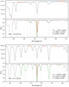 |
Fig. A.1. Fit performed to the Fe I 5044.21 Å and Fe II 5197.58 Å lines from one of the Sun spectra obtained by observing Ceres with HIRES. The top panels in both plots show the continuum fitting procedure, where the red dots are the final points selected for the fitting of the 2nd degree polynomial (blue line). Bottom panels: line fitting procedure. The gray lines are the absorption lines detected in the spectral range, and the green line the global fit to the data. The red region corresponds to the fit of the line l with its uncertainty, derived using the Gaussian parameters plus their uncertainties (quoted in the text). The green block represents the equivalent width. |
A.4. Equivalent width estimation
For each line l, the equivalent width is computed by integrating the line profile with parameters AI, wI, and σI, over the spectral region surrounding the line. The uncertainty in this value is estimated by changing the Gaussian parameters of the fit within 1σ of their uncertainty and then selecting the 16% and 84% percentiles of the distribution.
In order to assess the reliability of our method, we used it to estimate the equivalent width of the Sun, plus another seven stars considered to be solar twins, and compared them to the values obtained by Bedell et al. (2017), where the continuum estimation and line profile fitting were performed for each line by hand using the splot module of IRAF13. The results of out comparison, for the 8 stars, is shown in Fig. A.2, and Table A.1. The spectra were taken with the HIRES spectrograph (Vogt et al. 1994), and we used the same line list as in Bedell et al. (2017).
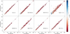 |
Fig. A.2. Comparison between the equivalent widths computed using SPECIES, against the values from Bedell et al. (2017). The number next to the names corresponds to the number of spectra available for each star. The color represents the uncertainty in the EW obtained with our method. |
Mean (μ), error in the mean (σμ), and standard deviation (σ) of the difference between the EWs computed by SPECIES, and from Bedell et al. (2017).
Appendix B: Supplementary figures and tables
 |
Fig. B.1. Correlations between all the parameters computed by SPECIES. Only a few of these are plotted in Fig. 11. This figure was generated using the final parameter values for all the stars in the EXPRESS sample. |
Line list used in the atmospheric parameters derivation.
Parameters derived with SPECIES for the stars included in interferometric and asteroseismology works.
Literature data for stars used in the comparison with interferometry and asteroseismology.
SPECIES results for the EXPRESS star sample.
Results for the Sun spectra.
Pearson correlation coefficient between all the parameters estimated by SPECIES, using the final values computed for the EXPRESS sample.
All Tables
Correspondance between equivalent evolutionary points (EEPs) and stellar evolutionary phase.
Linear fit parameters between the temperature obtained using the colour relations from Alonso et al. (1999) and SPECIES, with Teff, colour − Teff, SPECIES = a Teff, colour + b.
Mean and standard deviation for the parameters derived with SPECIES and how they change with the evolutionary stage.
Mean (μ), error in the mean (σμ), and standard deviation (σ) of the difference between the EWs computed by SPECIES, and from Bedell et al. (2017).
Parameters derived with SPECIES for the stars included in interferometric and asteroseismology works.
Literature data for stars used in the comparison with interferometry and asteroseismology.
Pearson correlation coefficient between all the parameters estimated by SPECIES, using the final values computed for the EXPRESS sample.
All Figures
|
Fig. 1. S/N distribution of our spectra for the EXPRESS sample. |
| In the text | |
|
Fig. 2. Fit performed using the EWComputation module to the blended lines Fe I 6297.80 Å and Fe II 6516.08 Å, from the giant star HIP9313 taken with CHIRON. The right-most text contains the values of A, μ, and σ, the amplitude, mean, and standard deviation, respectively, of the best Gaussian fit, along with their corresponding uncertainties eA, eμ, and eσ. The grey lines are the absorption lines detected in the spectral range, and the green line the global fit to the data. The red region corresponds to the fit of the line, l, with its uncertainty, derived using the Gaussian parameters plus their uncertainties. The green block represents the equivalent width, quoted in the left-most text. The full procedure is explained in Appendix A. |
| In the text | |
|
Fig. 3. H-R diagram of the giant star sample. The right panel is a close-up of the area where the stars in the sample are located. Open circles represent RGB stars and filled circles are HB stars. The tracks plotted have [Fe/H] = 0.0 and the different colours represent different phases in the stellar evolution. Grey lines represent the stages before the main sequence evolution (up to the TAMS, Table 2), and right after the end of core helium burning (TACHeB). For the meaning of the abbreviations and EEP number, see Table 2. |
| In the text | |
|
Fig. 4. Top panel: comparison between the radius measurement from SPECIES and from works using interferometry for the stars in our test sample. The black dotted line is the 1:1 relation. The inset correspond to a zoom of the squared regions. Bottom panel: difference SPECIES-literature. Uncertainties are computed considering both SPECIES and literature values ( |
| In the text | |
|
Fig. 5. Top panels: comparison between SPECIES and the asteroseismology studies for the stars in our test sample. The black dotted line in each panel is the 1:1 relation. Bottom panels: difference SPECIES-literature, same as in Fig. 4. The quoted text are the mean and standard deviation of the residuals for each quantity, and their percentage from the mean values. Surface gravity values were not given in Aguirre et al. (2020) and North et al. (2017), but were computed from their masses and radius. |
| In the text | |
|
Fig. 6. Comparison between SPECIES and the literature for the EXPRESS stars. Bottom panels: difference SPECIES-Literature. The errorbar shows the average uncertainties in the points. The quoted text are the mean and standard deviation of the residuals for each quantity, and their percentage from the mean values. |
| In the text | |
|
Fig. 7. Comparison between log g and log gtri. The black dashed line represents the 1:1 relation. |
| In the text | |
|
Fig. 8. Giant star classification, using the prescription from Collier Cameron et al. (2007), described in Sect. 3.1. The red line is the boundary between the dwarf and giant stars region. Points falling in the grey area are classified as dwarf stars. |
| In the text | |
|
Fig. 9. Comparison between temperature computed with the photometric relations from Alonso et al. (1999) and SPECIES. Orange line represents the linear fit to the data, quoted in the text. |
| In the text | |
|
Fig. 10. Histogram of the difference between the temperature from SPECIES and from photometry, before (left panel) and after correcting (right panel) via the linear fits. |
| In the text | |
|
Fig. 11. Correlations found between parameters derived in this work. The orange lines are the polynomial fits. Bottom panels are the residuals after subtracting the polynomial fits. The colour scale represents the median EEP for each target. Titles show the scatter in the residuals for the total sample (σT), stars in the RGB (σRGB) and in the HB (σHB). |
| In the text | |
|
Fig. 12. Mass-luminosity diagram for the EXPRESS sample. The colour scale represents the median EEP for each target. |
| In the text | |
|
Fig. 13. Distribution of the stellar evolutionary stage for the EXPRESS sample. The errorbars in each bin reflect the uncertainty in the EEP values, given by the 16% and 84% percentiles of the EEP distribution for each star. |
| In the text | |
|
Fig. 14. Distribution of some of the parameters derived by SPECIES, separated by their evolutionary stage. The red line corresponds to the HB distribution and the green line to the RGB distribution. The blue histogram represents the total of both distributions. |
| In the text | |
|
Fig. A.1. Fit performed to the Fe I 5044.21 Å and Fe II 5197.58 Å lines from one of the Sun spectra obtained by observing Ceres with HIRES. The top panels in both plots show the continuum fitting procedure, where the red dots are the final points selected for the fitting of the 2nd degree polynomial (blue line). Bottom panels: line fitting procedure. The gray lines are the absorption lines detected in the spectral range, and the green line the global fit to the data. The red region corresponds to the fit of the line l with its uncertainty, derived using the Gaussian parameters plus their uncertainties (quoted in the text). The green block represents the equivalent width. |
| In the text | |
|
Fig. A.2. Comparison between the equivalent widths computed using SPECIES, against the values from Bedell et al. (2017). The number next to the names corresponds to the number of spectra available for each star. The color represents the uncertainty in the EW obtained with our method. |
| In the text | |
|
Fig. B.1. Correlations between all the parameters computed by SPECIES. Only a few of these are plotted in Fig. 11. This figure was generated using the final parameter values for all the stars in the EXPRESS sample. |
| In the text | |
Current usage metrics show cumulative count of Article Views (full-text article views including HTML views, PDF and ePub downloads, according to the available data) and Abstracts Views on Vision4Press platform.
Data correspond to usage on the plateform after 2015. The current usage metrics is available 48-96 hours after online publication and is updated daily on week days.
Initial download of the metrics may take a while.