| Issue |
A&A
Volume 646, February 2021
|
|
|---|---|---|
| Article Number | A75 | |
| Number of page(s) | 31 | |
| Section | Cosmology (including clusters of galaxies) | |
| DOI | https://doi.org/10.1051/0004-6361/202038845 | |
| Published online | 10 February 2021 | |
Effects of observer peculiar motion on the isotropic background frequency spectrum: From the monopole to higher multipoles
1
INAF, Istituto di Radioastronomia, Via Piero Gobetti 101, 40129 Bologna, Italy
e-mail: This email address is being protected from spambots. You need JavaScript enabled to view it.
2
CNR, Istituto di Scienze Marine, Via Piero Gobetti 101, 40129 Bologna, Italy
3
Dipartimento di Fisica e Scienze della Terra, Università di Ferrara, Via Giuseppe Saragat 1, 44122 Ferrara, Italy
4
INFN, Sezione di Bologna, Via Irnerio 46, 40127 Bologna, Italy
5
INGV, Sezione Roma 2, Via di Vigna Murata 605, 00143 Roma, Italy
Received:
4
July
2020
Accepted:
9
November
2020
Abstract
Context. The observer peculiar motion produces boosting effects in the anisotropy pattern of the considered background with frequency spectral behaviours related to its frequency spectrum.
Aims. We study how the frequency spectrum of the background isotropic monopole emission is modified and transferred to the frequency spectra at higher multipoles, ℓ. We performed the analysis in terms of spherical harmonic expansion up to a certain value of ℓmax, for various models of background radiation, spanning the range between the radio and the far-infrared.
Methods. We derived a system of linear equations to obtain the spherical harmonic coefficients and provide the explicit solutions up to ℓmax = 6. These are written as linear combinations of the signals at N = ℓmax + 1 colatitudes. We take advantage of the symmetry property of the associated Legendre polynomials with respect to π/2, which allows for the separation of the system into two subsystems: (1) for ℓ = 0 and even multipoles and (2) for odd multipoles. This improves the accuracy of the solutions with respect to an arbitrary choice of the adopted colatitudes.
Results. We applied the method to different types of monopole spectra represented in terms of analytical or semi-analytical functions, that is, four types of distortions of the photon distribution function of the cosmic microwave background and four types of extragalactic background signals superimposed onto the cosmic microwave background’s Planckian spectrum, along with several different combinations of these types. We present our results in terms of the spherical harmonic coefficients and of the relationships between the observed and the intrinsic monopole spectra, as well as in terms of the corresponding all-sky maps and angular power spectra. For certain representative cases, we compare the results of the proposed method with those obtained using more computationally demanding numerical integrations or map generation and inversion. The method is generalized to the case of an average map composed by accumulating data taken with sets of different observer velocities, as is necessary when including the effect of the observer motion relative to the Solar System barycentre.
Conclusions. The simplicity and efficiency of the proposed method can significantly alleviate the computational effort required for accurate theoretical predictions and for the analysis of data derived by future projects across a variety of cases of interest. Finally, we discuss the superposition of the cosmic microwave background intrinsic anisotropies and of the effects induced by the observer peculiar motion, exploring the possibility of constraining the intrinsic dipole embedded in the kinematic dipole in the presence of background spectral distortions.
Key words: diffuse radiation / cosmic background radiation / methods: analytical
© ESO 2021
1. Introduction
The peculiar motion of an observer relative to an ideal reference frame at rest with respect to the cosmic background in a given frequency band, produces boosting effects in the anisotropy patterns at low multipoles with frequency spectral behaviours related to the spectrum of the isotropic monopole emission. The largest effect is on the dipole, that is, on the anisotropy at the ℓ = 1 multipole, which is mainly attributed to the solar system barycentre motion. The study of the dipole anisotropy spectrum is an alternative way to the achievement of absolute measurements for extracting information about the background monopole spectrum. This approach was originally proposed by Danese & De Zotti (1981) within the framework of cosmic microwave background (CMB) spectral distortions that possibly occurred in the cosmic plasma at different epochs. This method has been exploited by Balashev et al. (2015) in the context of future CMB anisotropy missions and, in particular, by De Zotti et al. (2016) with the aim of improving the characterization of the cosmic infrared background (CIB) spectrum. Numerical simulations have been performed to assess the impact of instrumental performance, potential residuals from imperfect foreground subtraction, and relative calibration uncertainties in the reconstruction of the types of signals described above (Burigana et al. 2018). This differential approach has been investigated to be applied to the analysis of the redshifted 21 cm line (Slosar 2017) and of its diurnal pattern in drift-scan observations (Deshpande 2018). Recent predictions of the cosmic dipole from four types of imprints that are expected from (or associated with) cosmological reionization – the diffuse free-free (FF) emission, the Comptonization distortion, the redshifted 21 cm line, and the radio extragalactic background, along with combinations of these types – have been presented by Trombetti & Burigana (2019).
In this work, we carry out an analysis of the effect of the observer peculiar motion on the frequency spectra of the monopole and of the anisotropy patterns at higher multipoles for the monopole component of various types of background radiation, ranging from the radio to the far-infrared (far-IR). For a blackbody spectrum, the amplitude of this effect decreases as βℓ at increasing ℓ, where β ≪ 1 is the module of the dimensionless peculiar velocity of the observer, which is defined by the vector β = v/c, c being the speed of light.
In general, the vector β is the sum of an almost constant component, βC, that is due to the motion of the Solar System barycentre with respect to the cosmic background and of a time varying component, βV = βV(t), which is due to the motion of the observer relative to the Solar System barycentre reference frame. For ground-based or sub-orbital experiments, βV is given by the combination of the motions of the Earth around the Solar System barycentre (βES ≃ 10−4) and of the experimental equipment on the Earth’s surface (βEE ≃ 1.7 × 10⁻⁶ for an experiment located at the Earth equator). For past, planned, and proposed CMB space missions, βV is given by the combination of the motion of the Earth or of the second Lagrangian point of the Sun-Earth system (L2) around the Solar System barycentre (βL2 ≃ 1.01 βES) and of the motion of spacecraft around the Earth or around L2, according to the adopted trajectory. For example, the typical spacecraft velocity around L2 is βL ≃ 1.7 × 10⁻⁶ for a Lissajous ‘orbit’ with a ‘radius’ of ≃3 × 10⁵ km described over a timescale of around six months. We note that the Solar System motion around the Galactic centre and the presence of local Universe gravitational fields imply time variations of β, but they can be neglected within the typical duration, τS, of a survey. For example, in the approximation of a uniform circular motion of the Solar System around the Galactic centre, with a rotation period P = 2π/ω ≃ 2.4 × 10⁸ yr and a velocity vSG ≃ 220 km s−1, that is, βSG ≃ 7.3 × 10⁻⁴, the relative variation of the velocity at a timescale of τS ≃ 5 yr is ΔvSG/vSG = ΔβSG/βSG ≃ ω2 ⋅ (vSG/ω) ⋅ τS/vSG = ω τS ≃ 1.3 × 10⁻⁷.
For numerical estimates, we will typically assume that the CMB dipole is due to velocity effects only and we neglect the modulation of β introduced by the contribution of βV. After the correction for the spacecraft motion around the Solar System barycentre, the nominal CMB dipole amplitude according to the Planck 2015 results (Planck Collaboration I 2016; Planck Collaboration V 2016; Planck Collaboration VIII 2016) is Adip = (3.3645 ± 0.002) mK. When using the Low Frequency Instrument alone (Planck Collaboration II 2020), the most recent analysis of the Planck 2018 results gives an almost identical value of Adip as in the 2015 release. On the other hand, when including, again, the High Frequency Instrument, the analysis of the Planck 2018 results gives Adip = (3.36208 ± 0.00099) mK (Planck Collaboration III 2020; Planck Collaboration I 2020), which is a slightly lower value. These results are clearly compatible within the errors. Based on a joint analysis (Fixsen 2009) of the data from the Far Infrared Absolute Spectrophotometer (FIRAS) on board the Cosmic Background Explorer (COBE) and from the Wilkinson Microwave Anisotropy Probe (WMAP), we adopt T0 = (2.72548 ± 0.00057) K for the current CMB effective temperature in the blackbody spectrum approximation, where  gives the current CMB energy density with a = 8πI3k4/(hc)3, I3 = π4/15, k and h the Boltzmann and Planck constants. We use the velocity vC = (369.82 ± 0.11) km s−1 given in Table 3 of Planck Collaboration I (2020), that is, β = βC = vC/c ≃ 1.2336 × 10⁻³ ≃ Adip/T0, to characterise the velocity of the Solar System barycentre with respect to the cosmic background.
The main contribution to the modulation of β coming from βV(t), which produces an effect amounting to ≃8.1% of the global signal, is derived from the component of the observer motion due to the revolution of the Earth or of L2 around the Solar System barycentre (see above estimates).
We study the effect of peculiar motion in terms of spherical harmonic expansion up to a certain value of ℓmax. In this way, we introduce a relative error in the prediction of the effect at a given ℓ that strongly decreases with ℓmax. Neglecting the contributions from higher orders, the dipole anisotropy spectrum was estimated as the difference between the signal measured in the direction of motion and in its perpendicular direction (Danese & De Zotti 1981), namely, in terms of a very simple linear combination of the signals in two specific directions. In this work, we show how this concept can be generalized to derive the frequency behaviour of the anisotropy pattern up to higher multipoles. We provide both a recipe and explicit solutions that can be directly used for accurate and swift theoretical predictions of the individual multipole patterns and of the global pattern, allowing us to bypass the need for more computationally demanding approaches that are based on delicate numerical integrations or on map generation and inversion.
In Sect. 2, we introduce the adopted formalism and the set of equations we aimed to solve. We provide the explicit equations and solutions up to ℓmax = 6 in Sect. 3 and ℓmax = 4 in Sect. 5 in order to point out some general properties of the solutions. In Sects. 4 and 6, we work out these solutions for the particular case of a blackbody spectrum to make clear their simple link with the contributions coming from the various orders of β. In some cases, we show their equivalence with the corresponding explicit exact solution at the order of β corresponding to ℓmax. In Sects. 7 and 8, we discuss the solutions up to low ℓmax, that is, ℓmax = 1 and 2, derived using just two or three colatitudes. Some remarks linking the general properties of the found solutions at various ℓmax with the monopole spectrum integration and differentiation are given in Sect. 9. The main applications and results of the proposed method are presented in Sect. 10 for eight specific types of background: we give concise presentations of the monopole spectrum models adopted in this study, we describe the main features of the found solutions and, for two very different cases, we compare them with the results based on a numerical integration. Some applications to combinations of signals are discussed in Sect. 11. In Sect. 12, we briefly present a set of results related to all-sky maps and angular power spectra, also for the purpose of comparison with previous analyses based on map generation and inversion. In Sect. 13, we discuss how the developed method can be directly generalized from the case of maps obtained with a constant observer velocity to the case of maps derived from the average of data taken with a set of different observer velocities, as, for example, in the case of β modulated by βV(t). In Sect. 14, we focus on the global pattern at microwave frequencies, discussing the superposition of the CMB intrinsic anisotropies and of the effects induced by the observer peculiar motion. The possibility of constraining the intrinsic dipole embedded in the kinematic dipole in the presence of CMB spectral distortions is then discussed in Sect. 15. Finally, in Sect. 16, we draw our main conclusions. Some technical aspects are provided in the three sections of the appendix.
2. Theoretical framework and formalism
The peculiar velocity effect on the frequency spectrum can be evaluated on the whole sky using the complete description of the Compton-Getting effect (Forman 1970). This is based on the Lorentz invariance of the photon distribution function. In this work, we are interested in the effects induced on the monopole (or global) signal that, by definition, is isotropic in an ideal reference frame at rest with respect to the CMB or, more generally, to the cosmic background under consideration. In principle, the CMB and the other cosmic backgrounds provide information on processes that possibly occurred at different epochs or that are differently weighted for a range of redshift shells. Thus, the above ideal reference frame should correctly refer to the corresponding cosmic phase.
At a given ν, the photon distribution function, ηBB/dist, for the considered type of spectrum needs to be computed with the frequency multiplied by the product  . The notation ‘BB/dist’ stands for a blackbody spectrum or for any type of non-blackbody signal (or for combinations of signals). This accounts for all the possible sky directions, which are defined by the unit vector
  , relative to the peculiar velocity of the observer, which is defined by the vector β in the reference frame at rest with respect to the considered cosmic background. This includes all the orders in β and the link with the geometrical properties induced at each multipole. We study the effect in terms of equivalent thermodynamic temperature, Tth(ν), defined as the temperature of the blackbody having the same η(ν) at the frequency ν,
 (1)
(1)
The observed signal map is then given by (Burigana et al. 2018)
 (2)
(2)
where  with
with  , x = hν/(kTr) and Tr = T0(1 + z) are the redshift invariant dimensionless frequency and the redshift-dependent effective temperature of the CMB.
The unit vector  is associated to the polar coordinates θ (colatitude) and ϕ (longitude). The function
  can be expanded in spherical harmonics. We adopt a reference system with the z axis parallel to the observer velocity and we can then simply replace β with β in the above dependencies. Thus,
 (3)
(3)
where Yℓ, m(θ, ϕ) are the spherical harmonics related to the associated Legendre polynomials,  , and the coefficients aℓ, m(ν, β) contain information on the background spectrum and the observer velocity.
In the adopted reference system, the isotropy of the background monopole, or, equivalently, of η, implies that  depends on θ but not on ϕ. Thus, in Eq. (3), we can take only the terms with m = 0 and in this case,
  , where
  are the renormalized associated Legendre polynomials:
 (4)
(4)
In general, for a real function, the coefficients of the spherical harmonics expansion with m > 0 are related to the coefficients with m < 0 by the relation  , where the index denotes the complex conjugation. We note that for this problem and with the adopted reference system with the z axis parallel (or antiparallel) to the observer velocity, we are interested only in the non-vanishing coefficients with m = 0, but, in general, we can also see that the coefficients aℓ, m with m ≠ 0 do not vanish. The publicly available tools allow us to efficiently compute the aℓ, m passing from a reference system to another (see Górski et al. 2005).
Formally, the coefficients aℓ, m(ν, β) can be computed through an inversion of Eq. (3):
![Mathematical equation: $$ \begin{aligned} a_{\ell ,m} (\nu , \beta )&= \int _{\theta =0}^\pi \int _{\phi =0}^{2\pi } T_{\rm th}^\mathrm{BB/dist} (\nu , \theta , \phi , \beta ) \mathrm{e}^{-\mathrm{i}m\phi } {\tilde{P}}_\ell ^m (\mathrm{cos} \, \theta ) \, \mathrm{sin} \, \theta \, \mathrm{d}\theta \, \mathrm{d}\phi \, \nonumber \\&= \int _{\theta =0}^\pi \int _{\phi =0}^{2\pi } \left[{ T_{\rm th}^\mathrm{BB/dist} (\nu , \theta , \phi , \beta ) - T_{\rm th}^\mathrm{BB/dist,rest} (\nu ) }\right]\\&\quad \times \mathrm{e}^{-\mathrm{i}m\phi } {\tilde{P}}_\ell ^m (\mathrm{cos} \, \theta ) \, \mathrm{sin} \, \theta \, \mathrm{d}\theta \, \mathrm{d}\phi + a_{\ell ,m}^\mathrm{rest} (\nu ), \nonumber \end{aligned} $$](/articles/aa/full_html/2021/02/aa38845-20/aa38845-20-eq17.gif) (5)
(5)
where  is evaluated through Eq. (2) and m = 0. In the last part of Eq. (5),
  and
and  are evaluated in the background rest frame, that is, these are the intrinsic spherical harmonics expansion coefficients and the intrinsic (isotropic) background monopole expressed in equivalent thermodynamic temperature. For this problem,
  does not vanish only for ℓ = 0. This form in Eq. (5) is useful in the numerical computation (see also Sect. 10.1) because the integrand function becomes the difference between the equivalent thermodynamic temperatures in the reference frames in motion and at rest with respect to the background. For a general background spectrum, this approach requires a delicate and computationally demanding integration over θ. For a small β, it could be difficult to achieve the extreme precision needed to characterize the fine and small details of spectral features. We can instead consider Eq. (3) with m = 0 for a set of N directions, namely, of colatitudes θi with i = 0, N − 1, to construct a linear system of N equations in the N unknowns aℓ, 0(ν, β), with ℓ = 0, N − 1, that can be solved given the corresponding N values of
  , provided that the determinant of the system coefficient matrix does not vanish. The solutions for the unknowns aℓ, 0(ν, β) can be then written as linear combinations of N signals,
  , that are evaluated for a given background monopole at N colatitudes.
With this simple scheme, we can fully characterize the observed signal map  up to the desired multipole component ℓmax = N − 1. Let us assume, as a rule of thumb, that the amplitude of this effect decreases at increasing multipole as βℓ ⋅ p, with p ≈ 1. The value appropriate to the case of a blackbody spectrum is p = 1, as mentioned in Sect. 1, while, in general, the effective scaling with ℓ is frequency-dependent and related to the monopole spectrum shape, as discussed in next sections. Considering a spherical harmonic expansion up to ℓmax leads to neglect the contributions from ℓ > ℓmax. Thus, given the above scaling, the relative error in the computation of the effect at a given ℓ ≤ ℓmax is, at most, on the order of β(ℓmax − ℓ + j) ⋅ p. For a generic choice of the N colatitudes, we simply have j = 1. Since β is on the order of 10−3, adopting ℓmax = 6, we expect to achieve an extremely high numerical accuracy that is sufficient for any application even in the very distant future; whereas, setting ℓmax = 4 can be adequate for predicting the corresponding multipole patterns as part of the analysis in forthcoming and planned (or proposed) surveys since no relevant error is introduced by neglecting the contributions at higher multipoles. In general, an accuracy up to any desired order can be then achieved with this approach by just computing
  in only a relatively small number of sky directions, N = ℓmax + 1.
We note that  and that for ℓ = 0, and for even ℓ, the associated Legendre polynomials
  are symmetric with respect to θ = π/2, whereas for odd ℓ, they vanish at θ = π/2 and are antisymmetric with respect to θ = π/2. This suggests that the linear system of N equations using θ = π/2 and pairs of colatitudes symmetric with respect to θ = π/2 are expected satisfy the following properties: (i) for θ = π/2, all the coefficients multiplying aℓ, 0 are null for odd ℓ; (ii) for each pair of colatitudes – if ℓ is even, the coefficient multiplying aℓ, 0 is the same, whereas, it is the opposite result for odd ℓ.
As made evident in the next sections, these properties can be used to significantly simplify the explicit solution of the system because they allow us to combine the equations into two separate subsystems: (1) (N − 1)/2 + 1 equations for aℓ, 0, with ℓ = 0 and even ℓ and (2) (N − 1)/2 equations for aℓ, 0 with odd ℓ. For even ℓmax, a choice of odd N = ℓmax + 1 colatitudes θi that satisfies the above symmetry implies j = 2 (instead of 1) for even ℓ in the scaling, β(ℓmax − ℓ + j) ⋅ p, of the relative error of the method (see also the discussion at the end of Appendix A). For odd ℓmax, the system can be built with N = ℓmax + 1 colatitudes θi as above, but avoiding the inclusion of π/2. The system can be split into two separate subsystems of N/2 equations: (1) for ℓ = 0 and even ℓ and (2) for odd ℓ; and in this case, j = 2 for odd ℓ (see also Sect. 7 and the discussion at the end of Sect. 8). This property allows us to achieve a significant improvement in accuracy with respect to a generic choice of the N colatitudes θi.
3. Explicit solutions up to ℓmax= 6
Explicitly expanding  in spherical harmonics up to ℓmax = 6, we get
 (6)
(6)
where we omit, for simplicity, the dependence of  on ν, θ and β and the dependencies of aℓ, 0 on ν and β.
To write the linear system of seven equations, we are able to choose among infinite possibilities, and the explicit form of the system (but not the solution up to the adopted maximum multipole) depends on the specific choice. Among the possible choices satisfying the symmetry properties described above, we selected a set of colatitudes θi such that the values of cos θi are rational numbers or just involve  in order to simplify the algebra: θi = 0, π/4, π/3, π/2, (2/3)π, (3/4)π, and π.
After a series of calculations, we derived the corresponding linear system. We obtain
 (7)
(7)
 (8)
(8)
 (9)
(9)
 (10)
(10)
 (11)
(11)
 (12)
(12)
 (13)
(13)
Equations (7)–(13) constitute the linear system that is to be solved; and the determinant of the coefficients of the system matrix, ≃ − 0.303, does not vanish. We can solve the system using the methods of elimination and substitution.
As anticipated, we can combine the above equations to split the system into two subsystems. By adding the left and right sides of Eqs. (7) and (13), of Eqs. (8) and (12), and of Eqs. (9) and (11), we get three equations which, complemented using Eq. (10), form a linear system involving only the four unknowns aℓ, 0 with ℓ = 0 and even ℓ. We can solve it by substitution. Equation (10) allows us to express  as a combination of
  , a2, 0, a4, 0, and a6, 0 to be put in the other three equations. From the first one, we then express a2, 0 as a combination of
  ,
,  ,
,  , a4, 0, and a6, 0 to be put in the two other remaining equations. We then represent a4, 0 as a combination of
  ,
,  ,
,  ,
,  ,
,  , and a6, 0, which allows us to derive first the solution for a6, 0:
![Mathematical equation: $$ \begin{aligned} a_{6,0} =&\frac{64}{693} \sqrt{\frac{4\pi }{13}} \Bigl [ \left({T_{\rm th}^\mathrm{BB/dist} (\theta =0) + T_{\rm th}^\mathrm{BB/dist} (\theta =\pi ) }\right) \\& - 6\left({T_{\rm th}^\mathrm{BB/dist} (\theta =\pi /4) + T_{\rm th}^\mathrm{BB/dist} (\theta =(3/4)\pi )}\right)\nonumber \\& + 8 \left({T_{\rm th}^\mathrm{BB/dist} (\theta =\pi /3)+T_{\rm th}^\mathrm{BB/dist} (\theta =(2/3)\pi )}\right)\nonumber \\& - 6 T_{\rm th}^\mathrm{BB/dist} (\theta =\pi /2) \Bigr ]. \nonumber \end{aligned} $$](/articles/aa/full_html/2021/02/aa38845-20/aa38845-20-eq49.gif) (14)
(14)
As suggested in the introduction, a6, 0 is written in terms of a linear combination of the set of values of  computed for the seven adopted colatitudes. With substitution, we subsequently derive the solution for a4, 0, a2, 0 and, finally, for a0, 0:
![Mathematical equation: $$ \begin{aligned} a_{4,0}&=\frac{8}{385}\sqrt{\frac{4\pi }{9}}\Bigl [{9\left({T_{\rm th}^\mathrm{BB/dist}(\theta =0)+T_{\rm th}^\mathrm{BB/dist}(\theta =\pi )}\right)}\\&\quad {- 10 \left({T_{\rm th}^\mathrm{BB/dist}(\theta =\pi /4)+T_{\rm th}^\mathrm{BB/dist}(\theta =(3/4)\pi )}\right)}\nonumber \\&\quad {-16\left({T_{\rm th}^\mathrm{BB/dist}(\theta =\pi /3)+T_{\rm th}^\mathrm{BB/dist}(\theta =(2/3)\pi )}\right)} \nonumber \\&\quad {+34T_{\rm th}^\mathrm{BB/dist}(\theta =\pi /2)} \Bigr ], \nonumber \end{aligned} $$](/articles/aa/full_html/2021/02/aa38845-20/aa38845-20-eq51.gif) (15)
(15)
![Mathematical equation: $$ \begin{aligned} a_{2,0}&=\frac{1}{693}\sqrt{\frac{4\pi }{5}}\Bigl [{121\left({T_{\rm th}^\mathrm{BB/dist}(\theta =0)+T_{\rm th}^\mathrm{BB/dist}(\theta =\pi )}\right)}\\&\quad {+396\left({T_{\rm th}^\mathrm{BB/dist}(\theta =\pi /4)+T_{\rm th}^\mathrm{BB/dist}(\theta =(3/4)\pi )}\right)}\nonumber \\&\quad {-352\left({T_{\rm th}^\mathrm{BB/dist}(\theta =\pi /3)+T_{\rm th}^\mathrm{BB/dist}(\theta =(2/3)\pi )}\right)}\nonumber \\&\quad {-330 T_{\rm th}^\mathrm{BB/dist}(\theta =\pi /2)}\Bigr ], \nonumber \end{aligned} $$](/articles/aa/full_html/2021/02/aa38845-20/aa38845-20-eq52.gif) (16)
(16)
![Mathematical equation: $$ \begin{aligned} a_{0,0}&=\frac{\sqrt{4\pi }}{630}\Bigl [{29\left({T_{\rm th}^\mathrm{BB/dist}(\theta =0)+T_{\rm th}^\mathrm{BB/dist}(\theta =\pi )}\right)}\\&\quad {+120\left({T_{\rm th}^\mathrm{BB/dist}(\theta =\pi /4)+T_{\rm th}^\mathrm{BB/dist}(\theta =(3/4)\pi )}\right)}\nonumber \\&\quad {+64\left({T_{\rm th}^\mathrm{BB/dist}(\theta =\pi /3)+T_{\rm th}^\mathrm{BB/dist}(\theta =(2/3)\pi )}\right)}\nonumber \\&\quad {+204T_{\rm th}^\mathrm{BB/dist}(\theta =\pi /2)}\Bigr ].\nonumber \end{aligned} $$](/articles/aa/full_html/2021/02/aa38845-20/aa38845-20-eq53.gif) (17)
(17)
Subtracting left and right sides of Eqs. (7) and (13), of Eqs. (8) and (12), and of Eqs. (9) and (11) we get three equations that form a linear system involving only the three unknowns aℓ, 0 with odd ℓ. From the difference between the first of these equations and the second equation multiplied by  and the difference between the first equation and the third equation multiplied by 2, we can write a system for a3, 0 and a5, 0. We first derive a5, 0
![Mathematical equation: $$ \begin{aligned} a_{5,0}=&\frac{32}{189}\sqrt{\frac{4\pi }{11}}\Bigl [{\left({T_{\rm th}^\mathrm{BB/dist}(\theta =0)-T_{\rm th}^\mathrm{BB/dist}(\theta =\pi )}\right)}\\&{-3\sqrt{2}\left({T_{\rm th}^\mathrm{BB/dist}(\theta =\pi /4)-T_{\rm th}^\mathrm{BB/dist}(\theta =(3/4)\pi )}\right)}\nonumber \\&{+4\left({T_{\rm th}^\mathrm{BB/dist}(\theta =\pi /3)-T_{\rm th}^\mathrm{BB/dist}(\theta =(2/3)\pi )}\right)}\Bigr ]\nonumber \end{aligned} $$](/articles/aa/full_html/2021/02/aa38845-20/aa38845-20-eq55.gif) (18)
(18)
and then, by substitution, a3, 0 and a1, 0
![Mathematical equation: $$ \begin{aligned} a_{3,0}&= \frac{2}{135} \sqrt{\frac{4\pi }{7}} \Bigl [ { 13 \left({T_{\rm th}^\mathrm{BB/dist} (\theta =0) - T_{\rm th}^\mathrm{BB/dist} (\theta =\pi ) }\right) } \\&\quad { + 15\sqrt{2} \left({T_{\rm th}^\mathrm{BB/dist} (\theta =\pi /4) - T_{\rm th}^\mathrm{BB/dist} (\theta =(3/4)\pi ) }\right) }\nonumber \\&\quad {- 56 \left({T_{\rm th}^\mathrm{BB/dist} (\theta =\pi /3) - T_{\rm th}^\mathrm{BB/dist} (\theta =(2/3)\pi ) }\right) } \Bigr ] \, , \nonumber \end{aligned} $$](/articles/aa/full_html/2021/02/aa38845-20/aa38845-20-eq56.gif) (19)
(19)
![Mathematical equation: $$ \begin{aligned} a_{1,0}&= \frac{1}{210} \sqrt{\frac{4\pi }{3}} \Bigl [ { 29 \left({T_{\rm th}^\mathrm{BB/dist} (\theta =0) - T_{\rm th}^\mathrm{BB/dist} (\theta =\pi ) }\right) } \\&\quad { + 60\sqrt{2} \left({T_{\rm th}^\mathrm{BB/dist} (\theta =\pi /4) - T_{\rm th}^\mathrm{BB/dist} (\theta =(3/4)\pi ) }\right) }\nonumber \\&\quad {+ 32 \left({T_{\rm th}^\mathrm{BB/dist} (\theta =\pi /3) - T_{\rm th}^\mathrm{BB/dist} (\theta =(2/3)\pi ) }\right) } \Bigr ] \, . \nonumber \end{aligned} $$](/articles/aa/full_html/2021/02/aa38845-20/aa38845-20-eq57.gif) (20)
(20)
We note that the structure of the solutions for aℓ, 0 for ℓ = 0, and even ℓ, involving the sums of  at pairs of colatitudes symmetric with respect to π/2 and
  at π/2, as well as the structure of the solutions for odd ℓ, involving the differences of
  at pairs of colatitudes symmetric with respect to π/2, reflect the symmetry and antisymmetry properties that are discussed at the end of Sect. 2, together with the corresponding implications for the system solution accuracy.
The solutions expressed in Eqs. (14)–(20) can be compared with each of the Eqs. (7)–(13) for a given colatitude θi: as expected, the sum of products of the various coefficients that multiply aℓ, 0, for ℓ = 0, 6, in the equation for  with the coefficients in Eqs. (14)–(20) that multiply
  gives exactly one. Remarkably, except for θi = π/2, where only ℓ = 0 and the even multipoles contribute to
  , for all the other colatitudes θi the above sum is equally contributed for one half by ℓ = 0 and by the even multipoles and for one half by the odd multipoles. This is another property related to the symmetry with respect to π/2 of the set of colatitudes adopted.
4. Solutions for a blackbody up to ℓmax= 6
Let us consider the specific case of the CMB, assumed to ideally exhibit a blackbody monopole spectrum with an effective temperature, T0, in the CMB rest frame. In this case, the photon distribution function is
 (21)
(21)
Equation (2) then gives the well-known expression
 (22)
(22)
with x′ = hν′/(kTr), highlighting that  does not depend on ϕ nor on ν.
The observed CMB effective temperature averaged over the full sky, T0, obs, is given by
 (23)
(23)
For an observer at rest with respect to the CMB, β = 0 and then the substitution of the integration variable, θ, with a new variable, w = cos θ, obviously gives T0, obs = T0 and implies that in the expansion represented by Eq. (3), as specified by Eq. (6), the only non-vanishing contribution to T0, obs comes from a term associated to the multipole coefficient a0, 0. Since  ,
,  .
.
For an observer in motion with respect to the CMB, β ≠ 0 and T0, obs can be calculated by simply substituting the integration variable, θ, with w = 1 − βcos θ. We get
 (24)
(24)
as already reported in Lucca et al. (2020) (see also Chluba 2011; Dai & Chluba 2014). By replacing ln[(1 + β)/(1 − β)] with its expansion in Taylor’s series up to β7, that is, with 2[β + (1/3)β3 + (1/5)β5 + (1/7)β7], we find:
![Mathematical equation: $$ \begin{aligned} T_{\rm 0,obs} = \frac{1}{2} (1-\beta ^2)^{1/2} T_0 \cdot 2 \cdot [1 + (1/3)\beta ^2 + (1/5)\beta ^4 + (1/7)\beta ^6]. \end{aligned} $$](/articles/aa/full_html/2021/02/aa38845-20/aa38845-20-eq71.gif) (25)
(25)
We now specify the coefficients, aℓ, 0, given by Eqs. (14)–(20) to the blackbody case using Eq. (22) to compute  at the seven considered colatitudes. After solving the algebra, we get
 (26)
(26)
 (27)
(27)
 (28)
(28)
 (29)
(29)
and
 (30)
(30)
 (31)
(31)
 (32)
(32)
In the above expressions, the factor (1 − β2)1/2T0 clearly comes from Eq. (22) while the three factors in the denominator come from the choice of the pairs of colatitudes θ symmetric to π/2, that have been set to 0 and π, π/4 and (3/4)π, π/3, and (2/3)π. We observe also that, because of the adopted ℓmax = 6 and the separation of the system into two subsystems, the solutions for  and
and  (see Eqs. (26) and (30)) do not show at numerator additional terms coming from higher multipoles, while they appear in the solutions for
  for ℓ ≤ 4 (see Eqs. (27)–(29), (31) and (32)).
It is evident that the coefficients,  , do not depend on θ. Thus, the substitution of the integration variable θ with w = cos θ, in the expansion represented by Eq. (3) again gives T0, obs and implies that the only non-vanishing contribution comes from a term associated to the multipole coefficient
  . An expansion in Taylor’s series up to β6, gives 1/(1 − β2) = 1 + β2 + β4 + β6, 1/(2 − β2) = (1 + β2/2 + β4/4 + β6/8)/2, and 1/(4 − β2) = (1 + β2/4 + β4/16 + β6/64)/4. It is then simple to verify that, at the same order in β, Eq. (29) gives exactly the result expressed by Eq. (25), as is required, in principle.
Equation (5) allows us to analytically derive the aℓ, 0(ν, β) for any ℓ for relatively simple dependencies of  , as in the case of the blackbody spectrum, namely, for Eq. (22). The form of the integrand in θ involves only the function sin θ/(1 − βcos θ) multiplied by polynomials in cos θ and when substituting the integration variable θ with w = 1 − βcos θ, the integrand consists only of functions as 1/w and powers of w. We omit the tedious calculation at ℓ ≥ 2. Instead, for ℓ = 1, we get:
![Mathematical equation: $$ \begin{aligned} a_{1,0}^\mathrm{BB}&= 2\pi (1-\beta ^2)^{1/2} T_0 \int _{\theta =0}^\pi \frac{\mathrm{sin} \, \theta }{1-\beta \mathrm{cos} \, \theta } \sqrt{\frac{3}{4\pi }} \mathrm{cos} \, \theta \, \mathrm{d}\theta \\&= 2\pi \sqrt{\frac{3}{4\pi }} (1-\beta ^2)^{1/2} T_0 \frac{1}{\beta ^2} \left[{ \mathrm{ln} \frac{1+\beta }{1-\beta } -2\beta }\right]\nonumber , \end{aligned} $$](/articles/aa/full_html/2021/02/aa38845-20/aa38845-20-eq86.gif) (33)
(33)
where, by replacing ln[(1 + β)/(1 − β)] with its expansion in Taylor’s series up to β7, gives:
![Mathematical equation: $$ \begin{aligned} a_{1,0}^\mathrm{BB} = \sqrt{4\pi } \sqrt{3} (1-\beta ^2)^{1/2} T_0 [\beta /3+\beta ^3/5+\beta ^5/7]. \end{aligned} $$](/articles/aa/full_html/2021/02/aa38845-20/aa38845-20-eq87.gif) (34)
(34)
Performing a Taylor’s series expansion up to β6 for 1/(1 − β2), 1/(2 − β2) and 1/(4 − β2), it is simple to verify that at the same order in β, Eq. (32) for  gives precisely the result expressed by Eq. (34).
Finally, we remember that in Sect. 3 we discussed deriving both a0, 0 and a1, 0 by substitution in the last step of the calculation to solve the corresponding linear subsystem. Thus, the consistencies discussed above for T0, obs and  at the adopted order also represent a further verification of the derived algebraic solutions.
5. Explicit solutions up to ℓmax= 4
For many applications, a computation up to ℓmax = 4 suffice to get the relevant information. We then provide here simpler solutions based on N = 5 equations using the set of colatitudes 0, π/4, π/2, (3/4)π and π. This also allows us to explicitly focus on some of the mentioned properties of the proposed method.
We construct a system formed only by Eqs. (7), (8), (10), (12) and (13) ignoring the terms associated to a5, 0 and a6, 0, and we again solve it with the methods of elimination and substitution in a way similar to that described in Sect. 3. The solutions are
![Mathematical equation: $$ \begin{aligned} a_{4,0}&= \frac{8}{35} \sqrt{\frac{4\pi }{9}} \Bigl [ { \left({T_{\rm th}^\mathrm{BB/dist} (\theta =0) + T_{\rm th}^\mathrm{BB/dist} (\theta =\pi ) }\right) } \\&\quad { - 2 \left({T_{\rm th}^\mathrm{BB/dist} (\theta =\pi /4) + T_{\rm th}^\mathrm{BB/dist} (\theta =(3/4)\pi ) }\right) }\nonumber \\&\quad {+ 2 T_{\rm th}^\mathrm{BB/dist} (\theta =\pi /2) } \Bigr ] \nonumber , \end{aligned} $$](/articles/aa/full_html/2021/02/aa38845-20/aa38845-20-eq90.gif) (35)
(35)
![Mathematical equation: $$ \begin{aligned} a_{2,0}&= \frac{1}{21} \sqrt{\frac{4\pi }{5}} \Bigl [ { 5 \left({T_{\rm th}^\mathrm{BB/dist} (\theta =0) + T_{\rm th}^\mathrm{BB/dist} (\theta =\pi ) }\right) } \\&\quad { + 4 \left({T_{\rm th}^\mathrm{BB/dist} (\theta =\pi /4) + T_{\rm th}^\mathrm{BB/dist} (\theta =(3/4)\pi ) }\right) }\nonumber \\&\quad {- 18 T_{\rm th}^\mathrm{BB/dist} (\theta =\pi /2) } \Bigr ] \nonumber \, , \end{aligned} $$](/articles/aa/full_html/2021/02/aa38845-20/aa38845-20-eq91.gif) (36)
(36)
![Mathematical equation: $$ \begin{aligned} a_{0,0}&= \frac{\sqrt{4\pi }}{30} \Bigl [ { \left({T_{\rm th}^\mathrm{BB/dist} (\theta =0) + T_{\rm th}^\mathrm{BB/dist} (\theta =\pi ) }\right) } \\&\quad { + 8 \left({T_{\rm th}^\mathrm{BB/dist} (\theta =\pi /4) + T_{\rm th}^\mathrm{BB/dist} (\theta =(3/4)\pi ) }\right) }\nonumber \\&\quad {+12 T_{\rm th}^\mathrm{BB/dist} (\theta =\pi /2) } \Bigr ] \, . \nonumber \end{aligned} $$](/articles/aa/full_html/2021/02/aa38845-20/aa38845-20-eq92.gif) (37)
(37)
Next, we have
![Mathematical equation: $$ \begin{aligned} a_{3,0}&= \frac{2}{5} \sqrt{\frac{4\pi }{7}} \Bigl [ { \left({T_{\rm th}^\mathrm{BB/dist} (\theta =0) - T_{\rm th}^\mathrm{BB/dist} (\theta =\pi ) }\right) } \\&\quad { - \sqrt{2} \left({T_{\rm th}^\mathrm{BB/dist} (\theta =\pi /4) - T_{\rm th}^\mathrm{BB/dist} (\theta =(3/4)\pi ) }\right) } \Bigr ] \nonumber \, , \end{aligned} $$](/articles/aa/full_html/2021/02/aa38845-20/aa38845-20-eq93.gif) (38)
(38)
![Mathematical equation: $$ \begin{aligned} a_{1,0}&= \frac{1}{10} \sqrt{\frac{4\pi }{3}} \Bigl [ { \left({T_{\rm th}^\mathrm{BB/dist} (\theta =0) - T_{\rm th}^\mathrm{BB/dist} (\theta =\pi ) }\right) } \\&\quad { + 4 \sqrt{2} \left({T_{\rm th}^\mathrm{BB/dist} (\theta =\pi /4) - T_{\rm th}^\mathrm{BB/dist} (\theta =(3/4)\pi ) }\right) } \Bigr ] \, \nonumber . \end{aligned} $$](/articles/aa/full_html/2021/02/aa38845-20/aa38845-20-eq94.gif) (39)
(39)
While the structure of the solutions expressed by Eqs. (35)–(39) is analogous to the structure of Eqs. (15)–(17), (19) and (20), the different algebraic coefficients reflect the different choice adopted for the set of colatitudes.
6. Solutions for a blackbody up to ℓmax= 4
Specifying the coefficients, aℓ, 0, given by Eqs. (35)–(39) to the blackbody case (see Eq. (22)), we compute  at the five considered colatitudes and we obtain
 (40)
(40)
 (41)
(41)
 (42)
(42)
and
 (43)
(43)
 (44)
(44)
In this case (ℓmax = 4), the solutions for  and
and  do not show, in terms of the numerator, additional higher multipoles terms, as they appear at ℓ ≤ 2. The algebraic coefficients appearing in Eqs. (40)–(44) and in Eqs. (27)–(29), (31) and (32) are different, but these sets of equations give exactly the same solutions when the ratios of their polynomials in β are computed up to the order of β4. Analogously, Eq. (42) gives for T0, obs the same result of Eqs. (25) and (44) is equivalent to Eq. (34) when they are computed up to the same order of power in β.
7. Explicit solutions up to ℓmax= 2 and 1
It is helpful to write the solutions for low values of ℓmax.
From the N = 3 equations at the colatitudes 0, π/2 and π (Eqs. (7), (10), and (13)), ignoring the terms associated to aℓ, 0 for ℓ > 2, we get
![Mathematical equation: $$ \begin{aligned}&a_{2,0} = \frac{1}{3} \sqrt{\frac{4\pi }{5}} \Bigl [ { \left({T_{\rm th}^\mathrm{BB/dist} (\theta =0)+ T_{\rm th}^\mathrm{BB/dist} (\theta =\pi ) }\right) }\\&\qquad \quad {- 2 T_{\rm th}^\mathrm{BB/dist} (\theta =\pi /2) } \Bigr ] \nonumber , \end{aligned} $$](/articles/aa/full_html/2021/02/aa38845-20/aa38845-20-eq103.gif) (45)
(45)
![Mathematical equation: $$ \begin{aligned}&a_{1,0} = \frac{1}{2} \sqrt{\frac{4\pi }{3}} \Bigl [ { \left({T_{\rm th}^\mathrm{BB/dist} (\theta =0) - T_{\rm th}^\mathrm{BB/dist} (\theta =\pi ) }\right) } \Bigr ], \end{aligned} $$](/articles/aa/full_html/2021/02/aa38845-20/aa38845-20-eq104.gif) (46)
(46)
![Mathematical equation: $$ \begin{aligned}&a_{0,0} = \frac{\sqrt{4\pi }}{6} \Bigl [ { \left({T_{\rm th}^\mathrm{BB/dist} (\theta =0) + T_{\rm th}^\mathrm{BB/dist} (\theta =\pi ) }\right) } \\&\qquad \quad {+ 4 T_{\rm th}^\mathrm{BB/dist} (\theta =\pi /2) } \Bigr ].\nonumber \end{aligned} $$](/articles/aa/full_html/2021/02/aa38845-20/aa38845-20-eq105.gif) (47)
(47)
Using only N = 2 equations at the colatitudes 0 and π (Eqs. (7) and (13)), neglecting the terms at ℓ > 1, we have
![Mathematical equation: $$ \begin{aligned}&a_{1,0} = \frac{1}{2} \sqrt{\frac{4\pi }{3}} \Bigl [ { \left({T_{\rm th}^\mathrm{BB/dist} (\theta =0) - T_{\rm th}^\mathrm{BB/dist} (\theta =\pi ) }\right) } \Bigr ], \end{aligned} $$](/articles/aa/full_html/2021/02/aa38845-20/aa38845-20-eq106.gif) (48)
(48)
![Mathematical equation: $$ \begin{aligned}&a_{0,0} = \frac{\sqrt{4\pi }}{2} \Bigl [ { \left({T_{\rm th}^\mathrm{BB/dist} (\theta =0) + T_{\rm th}^\mathrm{BB/dist} (\theta =\pi ) }\right) } \Bigr ]. \end{aligned} $$](/articles/aa/full_html/2021/02/aa38845-20/aa38845-20-eq107.gif) (49)
(49)
With N = 2 equations but at the colatitudes 0 and π/2 (Eqs. (7) and (10)), which is clearly not symmetric with respect to π/2, instead we get:
![Mathematical equation: $$ \begin{aligned}&a_{1,0} = \sqrt{\frac{4\pi }{3}} \Bigl [ { \left({T_{\rm th}^\mathrm{BB/dist} (\theta =0) - T_{\rm th}^\mathrm{BB/dist} (\theta =\pi /2) }\right) } \Bigr ], \end{aligned} $$](/articles/aa/full_html/2021/02/aa38845-20/aa38845-20-eq108.gif) (50)
(50)
![Mathematical equation: $$ \begin{aligned}&a_{0,0} = \sqrt{4\pi } \Bigl [ { \left({T_{\rm th}^\mathrm{BB/dist} (\theta =\pi /2) } \right) } \Bigr ]. \end{aligned} $$](/articles/aa/full_html/2021/02/aa38845-20/aa38845-20-eq109.gif) (51)
(51)
8. On dipole estimations based on two colatitudes
As proposed by Danese & De Zotti (1981), a suitable and observationally intuitive approximation for the dipole spectrum can be expressed in terms of the difference of  in the direction of motion and in its perpendicular direction.
Equations (7) and (10) allow us to express this difference in terms of a combination of the coefficients aℓ, 0(ν, β) up to ℓmax = 6:
 (52)
(52)
Neglecting the contributions from ℓ > 1, Eqs. (50) and (52) are equivalent. We can also express the semi-difference in  measured in the direction of motion and in its opposite direction using Eqs. (7) and (13)
 (53)
(53)
and in leaving out the terms at ℓ > 1, Eq. (53) is equivalent to Eq. (48).
The estimation of a1, 0(ν, β) through the simple difference of  in only two directions can be performed using the two colatitudes θ = 0 and θ = π to automatically suppress the contributions from ℓ = 2 (and from higher even ℓ), as discussed at the end of Sect. 2. The same holds for any other pair of colatitudes symmetric with respect to π/2 (as can be derived, for example, by combining Eqs. (8) and (12) or Eqs. (9) and (11)). The solutions presented in Sect. 3 can instead be used to correct for the contributions from the odd terms at ℓ = 3 and 5 (and from the terms at even ℓ, when using Eq. (52)).
9. Solutions for aℓ, 0 and spectrum integration or differentiation
Equation (5) shows that the solution for a given aℓ, 0 is an integral of  over θ. Since β is very small, when θ spans in the interval [0, π], around π/2, the values of
  in the integrand come from frequency values in a small interval around ν/(1 − β2)1/2 (see Eq. (2) and the relation between ν and ν′), making the integral sensitive to the local variation of
  . Formally, the solutions expressed by Eqs. (14)–(20) and (35)–(39) can be regarded as definitions of sets of weights assigned to a small number of values of function
  in a given set of colatitudes, or corresponding frequencies, to compute the integrals that give the coefficients aℓ, m in Eq. (5).
To a first-order approximation, the dipole spectrum induced by the observer peculiar velocity is directly proportional to the first logarithmic derivative of the photon occupation number, η(ν), with respect to the frequency, ν (Danese & De Zotti 1981). This concept can be generalized to higher multipoles. Let us consider the partial derivative of Eq. (5) with respect to the frequency, ν. According to Leibniz’s rule, when performing the differentiation under the integral sign, a further multiplicative factor involving the product, β cos θ, enters in the integral over θ, other than factors depending on the form of η(ν). As is evident from Eq. (6), a further power of cos θ appears passing from ℓ to ℓ + 1 in the associated Legendre polynomials and, consequently, in the integrand function of aℓ, 0 (see Eq. (5)). Thus, the subsequent aℓ, 0(ν) at increasing ℓ is tightly related to the subsequent derivatives of η(ν) with respect to ν, or in other words, their frequency behaviours are particular sensitive to the local (in frequency space) monopole spectrum variation up to increasing derivative order.
It is interesting to note certain properties of the coefficients (or weights) in Eqs. (14)–(20), (35)–(39), (45)–(47), (48) and (49) that are related to the separation of odd and even multipoles in the system solution. As already discussed, this separation appears when we adopt sets of colatitudes θ symmetrically located around π/2. The central weight, applied to θ = π/2, is zero for odd ℓ but not for even ℓ. For angles θ symmetric with respect to π/2, the weights are opposite for odd ℓ and equal for even ℓ. The sum of the weights vanishes, except for ℓ = 0: in this case, the sum is exactly unit, when divided by the ‘normalization’ factor,  (see also Eq. (6)). These properties are identical to those satisfied by the weights for the centred approximations at a grid point for the generation of finite difference formulas on arbitrarily spaced grids for any order of derivative (Fornberg 1988, 1998). Furthermore, we note that the relative weights in Eqs. (45), (46), and (48) are equivalent to the relative weights for the centred approximations at a grid point for the second and first order of derivative, the relative weights in Eq. (49) are equivalent to the relative weights for the centred approximations at the halfway point for the zero order of derivative, while the relative weights in Eqs. (50) and (51) are equivalent to the relative weights for the one-sided approximations at a grid point for the first and zero order of derivative. The different level of approximation in the estimate of a1, 0 via Eqs. (52) and (53), neglecting terms at ℓ > 1, is clearly related to the different accuracies of the one-sided and centred scheme for numerical differentiation. Finally, the relative weights for a0, 0 in Eq. (47) are not equivalent to relative weights for the zero order of derivative of the schemes mentioned above. This is of increasing evidence in the weights of the solutions at ℓmax > 2. Remarkably, they do not satisfy the sign alternation appearing in the weights of the centred approximations at a grid point of finite difference formulas moving from the central node to the more external nodes. Indeed, they store the relations between the aℓ, 0 at different ℓ and the temperatures at the adopted set of colatitudes that originates from the system solution at the corresponding ℓmax (this is analogous to the ‘mixing’ of derivatives discussed above).
10. Monopole spectrum models and single signal results
The method described can be applied to any type of signal and to combinations of signals, provided that they are summed in terms of additive quantities, such as the photon distribution function, η, or the antenna temperature,
 (54)
(54)
In this work, we consider eight different types of monopole spectrum that can be represented in terms of analytical or semi-analytical functions.
We first focus on four types of signals characterized by a CMB-distorted photon distribution function, ηdist(ν) that is different from the blackbody, ηBB(ν), at the present temperature T0. We then consider four types of extragalactic background superimposed onto the CMB blackbody spectrum. We give only a concise description of the various models, referring to the literature for further information. On the other hand, we report the equations relevant for a clear connection with Sect. 14.
We first consider the signals that are more relevant (or essentially relevant) at low frequencies (radio domain) and then those that are relevant over a very wide frequency range (up to the far-IR) or more important at increasing frequency. We compare the results based on the proposed method (the solutions in Sect. 3) with the computation based on direct numerical integration (see Eq. (5) and the discussion in Sect. 10.1). For simplicity, we perform the comparison (see also Appendix A) only for two representative cases, which were chosen because they are very different with regard to the spectrum features.
The results are presented in terms of the following quantities:
– The difference, ΔTth, between the equivalent thermodynamic temperature of the intrinsic monopole spectrum for the adopted model and the CMB present temperature T0.
– The ratio,  , between the equivalent thermodynamic temperature of observed (see Eq. (6)) and intrinsic monopole, expressed in terms of the difference ΔR = R − RBB, where RBB ≃ (1−2.5362 × 10⁻⁷) is the same ratio but for the case of the blackbody, ηBB(ν), at the present temperature T0 (see Eqs. (23)–(25) and the discussion in Sect. 4).
– The coefficients aℓ, 0(ν, β) from ℓ = 1 to ℓmax = 6 (see Eqs. (14)–(16) and (18)–(20)) expressed in terms of their difference with the blackbody case (see Eqs. (26)–(28) and (30)–(32)).
10.1. Possible non-equilibrium imprint at low frequencies
An important extragalactic background signal that is much larger than the CMB background predicted for a blackbody spectrum at an equilibrium temperature in agreement with FIRAS results is observed at radio frequencies, in particular, below a few GHz (see e.g., Dowell & Taylor 2018). A signal excess could be also present at ≃3.3 GHz, as claimed by Singal et al. (2011) on the basis of the second generation of the Absolute Radiometer for Cosmology, Astrophysics, and Diffuse Emission (ARCADE 2) data. Models based on contributions by faint astrophysical sources, on interactions between dark matter (DM) and baryons, or on their combinations have been invoked to explain this background, possibly together with the pronounced absorption profile of the 21 cm redshifted line signal (see also Sect. 10.4), which has also been claimed by Bowman et al. (2018); see, for example, Seiffert et al. (2011), Barkana (2018), Muñoz & Loeb (2018), Ewall-Wice et al. (2018) and Mirabel (2019) (see also Subrahmanyan & Cowsik 2013; Hills et al. 2018; Sharma 2018).
Baiesi et al. (2020) proposed an alternative explanation of the signal excess in the low frequency background, involving a mechanism of stochastic frequency diffusion in the perspective of non-equilibrium statistical mechanics. The model implies a modification of the standard Kompaneets equation (Kompaneets 1957), explicitly considered by the authors in the limit that includes only the scattering, and a relaxation of the Einstein detailed balance relation. The resulting abundance of low frequency photons can be described by a stationary solution of the photon distribution function in the form:
![Mathematical equation: $$ \begin{aligned} \eta (\nu ) = \frac{1}{\mathrm{exp} \left[{\int ^\nu \mathrm{d}\nu^\prime \gamma (\nu^\prime )/D(\nu^\prime )}\right] - 1} = \frac{1}{e^{\psi (\nu )} - 1}, \end{aligned} $$](/articles/aa/full_html/2021/02/aa38845-20/aa38845-20-eq122.gif) (55)
(55)
where γ and D are frequency dependent friction and diffusion terms and the function ψ(ν) can be approximated by
 (56)
(56)
Subtracting from the global extragalactic background signal the contribution by extragalactic radio sources, for instance assuming the model by Gervasi et al. (2008a) with an amplification factor of ≃1.3 in the resulting background (see also Sect. 10.5), and comparing the residual background with their almost complete collection of cosmic background absolute temperature data, they found: ν0 ≃ 0.4 GHz for α = 3 (and T⋆ = T0 to fit high frequency data), ν0 ≃ 0.35 GHz, and α ≃ 3.36 using both ν0 and α as fit variables.
In Fig. 1, we show ΔTth, ΔR and the coefficients aℓ, 0(ν, β) for ℓ = 1, 6, expressed in terms of Δaℓ, 0, derived for the two sets of best-fit parameters according to the solutions in Sect. 3 and in one case, also on the basis of Eq. (5). The computations were performed in quadruple precision. We first carried out some tests with a simple Gaussian quadrature scheme (Press 1992), using various accuracy parameter values and point numbers (e.g., with the accuracy parameter (EPS) set to 10−9 and 2048 points), and compare the result with the explicit analytical solution for a blackbody: we find unreliable results above ℓ = 3 (or above ℓ = 4 provided that Eq. (5) is written as in the last equality). We then performed the numerical integration using the very accurate and efficient routine D01AJF of the Numerical Algorithms Group (NAG) Numerical Library, available only in double precision, setting integration accuracy parameters to the smallest values and increasing the number of sub-intervals used by the routine and the related workspace allocation. However, we verified that splitting the integral in terms of sums of integrals over subsets of the integration intervals does not improve the accuracy at all.
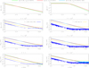 |
Fig. 1. ΔTth, ΔR and Δaℓ, 0 from ℓ = 1 to ℓmax = 6 for the considered non-equilibrium models. Solid lines (or dots) correspond to positive (or negative) values. Green and light blue lines are essentially superimposed up to ℓ = 4, where only one of the two lines can be appreciated. Their difference multiplied by a factor F to have values compatible with the adopted range is displayed by the blue lines. Yellow lines refer to the nominal integration error quoted by the routine D01AJF, again multiplied by the factor F. See also the legend and the text. |
There is very good agreement between the results found with the routine D01AJF and the solutions in Sect. 3 with ℓmax = 6 (particularly at lower multipoles, where the lines are superimposed and indistinguishable). Their differences are compatible with a combination of higher order terms, that is, beyond ℓ = 6, and integration errors, that are missing in the solutions in Sect. 3 and present in the numerical results, respectively. The two types of differences clearly appear, respectively, at lower frequencies, where the signal is higher and the relative integration error is lower, and at higher frequencies, where the signal is lower and the relative integration error is higher. We report also the nominal integration error quoted by the routine D01AJF: the comparison with the above differences suggests that this error is likely very conservative. In Appendix A, we provide some results derived adopting a much larger value of β that implies much larger signals, relatively higher contributions from higher multipoles, as well as relatively lower numerical integration errors: the analysis clearly supports the above interpretation.
Figure 1 shows that the typical power law shape of the intrinsic monopole spectrum, subsequent to the subtraction of the blackbody at the present temperature T0, is displayed also at higher multipoles, as already discussed in Trombetti & Burigana (2019) for the dipole. Remarkably, we find that the ratio, R, between observed and intrinsic monopole, ΔR in Fig. 1, is not frequency independent, as in the case of a blackbody, but exhibits a frequency dependence related to the assumed intrinsic monopole spectrum. At low frequencies, below ∼1 GHz, the values of ΔR are positive and with amplitudes comparable to |RBB − 1| or even larger.
10.2. Comptonization distortion and free-free diffuse emission
Many types of sources of photon and energy injections in cosmic plasma generates Comptonization distortions (Zel’dovich et al. 1972) via electron heating, and in ionizing the matter, they also produce FF distortions. Although these signatures can be generated both before (see e.g., Chluba & Sunyaev 2012) and after the cosmological recombination epoch (see e.g., Stebbins & Silk 1986; Danese & Burigana 1994), the cosmological reionization associated with the early formation phases of bound structures is the most remarkable source of these distortions. Two key parameters quantify the amplitudes of these imprints that for a given model, are tightly coupled. They are the Comptonization parameter, u, proportional to the global fractional energy exchange between matter and radiation in the cosmic plasma (for small distortions u ≃ (1/4)Δε/εi), and the FF distortion parameter, yB(x), defined by integrals over the relevant redshift interval. On the other hand, even in the context of the reionization process, a variety of astrophysical mechanisms can contribute to determine the final distortion levels (see e.g., De Zotti et al. 2016; Burigana et al. 2018, and references therein). The resulting distorted photon distribution function is well approximated by
![Mathematical equation: $$ \begin{aligned} \eta ^\mathrm{FF+C} \simeq \eta _{\rm i} + u {x / \phi _{\rm i} \,e^{x/\phi _{\rm i}} \over (e^{x/\phi _{\rm i}} - 1)^{2}} \left( {x/\phi _{\rm i} \over {\mathrm{tanh}[x/(2\phi _{\rm i})] }} - 4 \right) + \frac{{ y}_{B}(x)}{x^{3}}, \end{aligned} $$](/articles/aa/full_html/2021/02/aa38845-20/aa38845-20-eq124.gif) (57)
(57)
where ηi is the photon occupation number at the dissipation process initial time denoted with the subscript i. Neglecting other processes, ηi can be assumed to have a Planckian distribution at the initial temperature defined by ϕi = ϕ(zi) = (1 + Δε/εi)−1/4 ≃ 1 − u, that is, ηi = 1/(ex/ϕi − 1).
The global Comptonization distortion depends linearly on matter density, thus, assuming a uniform medium is not critical for computing u. Conversely, bremsstrahlung depends quadratically on matter density and, in the presence of a substantial intergalactic medium (IGM) matter density contrast, the FF distortion is amplified with respect to the case of a homogeneous medium (Cooray & Furlanetto 2004; Ponente et al. 2011; Trombetti & Burigana 2014) by a factor of ≃1 + σ2(z), that is,  , with σ2(z) as the baryonic matter variance related to the thermal properties of the DM particles.
Following Trombetti & Burigana (2019), we consider two pairs of different FF and Componization distortion models to identify a plausible range of possible distortions. We first consider the ionization history of Gnedin (2000), resulting in a Thomson optical depth τ that is fully consistent with recent Planck results, along with a fixed cut-off value kmax = 100. We coupled it with two different levels of Comptonization distortion, characterized by u = 10−7, which is very close to that derived in Burigana et al. (2008) for the Gnedin (2000) model and corresponds to an almost minimal energy injection consistent with the current constraints on τ, and by u = 2 × 10⁻⁶, a value that accounts for possible additional energy injections by a broad set of astrophysical phenomena.
At long wavelengths, λ = c/ν ≳ λ0 = 1.5 cm, yB is well-described by a linear dependence on log λ,  , while at λ = c/ν ≲ λ0 a quadratic dependence,
  , works better. The coefficients alin and blin are given in Appendix C of Trombetti & Burigana (2014): for the adopted model alin ≃ 3.292 × 10⁻⁹, blin ≃ 2.070 × 10⁻⁹. To allow for continuous derivatives of yB also at frequencies around the transition between the two regimes, thus avoiding to introduce spurious oscillations in the resulting aℓ, 0, we need to properly join the two representations. Combining them with exponential weights,
 (58)
(58)
with d = 3/2, is suitable to this purpose. A best-fit (see Table C.1 of Trombetti & Burigana 2014) gives aquad ≃ −4.657 × 10⁻¹⁰, bquad ≃ 1.210 × 10⁻⁹, cquad ≃ 2.841 × 10⁻⁹.
Larger FF distortions are expected from the integrated contribution of an ensemble of ionized halos at substantial redshifts, as in the model by Oh (1999) that predicts a value of yB ∼ 1.5 × 10⁻⁶ at ν ∼ 2 GHz. We then consider a second pair of models rescaling the above FF representation to yB(2 GHz) = 1.5 × 10⁻⁶, coupled with Comptonization distortions with u = 10−7 or 2 × 10⁻⁶.
In general, the frequency behaviour of yB is significantly less model dependent than its overall amplitude. A power law representation of yB with a single amplitude parameter is adopted, for simplicity, in Sect. 14. In this approximation
 (59)
(59)
where, assuming ζ ≃ 0.15, suitable values of AFF at low frequencies (several MHz ≲ ν ≲ some GHz) are respectively AFF ≃ 7.012 × 10⁻⁹ and 1.664 × 10⁻⁶ (Trombetti & Burigana 2019). Assuming the same slope but values of AFF multiplied by a proper factor, f, offers a reasonable approximation also at 30 GHz ≲ ν ≲ 100 GHz (on average we find f ∼ 0.578, while it ranges between ≃0.550 and ≃0.596). Of course, a better power law fit can be found jointly varying AFF and ζ according to the considered frequency range. As examples, for the first model at 10 MHz ≲ ν ≲ 1 GHz (or at 30 GHz ≲ ν ≲ 100 GHz) we find AFF ≃ 7.225 × 10⁻⁹ and ζ ≃ 0.143 (or AFF ≃ 5.236 × 10⁻⁹ and ζ ≃ 0.214). The adopted intrinsic monopole models are shown in Fig. 2 (top-left panel) in terms of ΔTth.
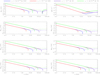 |
Fig. 2. ΔTth, ΔR and Δaℓ, 0 from ℓ = 1 to ℓmax = 6 for the considered combined Comptonization and diffuse FF distortion models. Solid lines (or dots) correspond to positive (or negative) values. See also the legend and the text. |
The results in Fig. 2 are derived multiplying yB in Eq. (58) by a damping function, exp(−(λ/λ1)d)exp(−(λ/λ2)d), which is relevant at very short wavelengths (λ1 = 0.09 cm and λ2 = 0.05 cm, corresponding to ≃333 GHz and 600 GHz) to make the results at ν ≳ 400 GHz dependent essentially only on the Comptonization term. This does not appreciably affect the results shown in the various panels of Fig. 2 at ν ≲ 400 GHz. On the other hand, while a better theoretical characterization of the FF emission at very high frequencies is required for a proper estimate in this context, we note that at ν ≳ 400 GHz the signal associated to the CIB, discussed in Sect. 10.7, dominates over the other terms at any multipole.
The differences, Δaℓ, 0, derived for these models are positive at low frequencies, where the FF term dominates, and negative at high frequencies, where the Comptonization prevails. The transition from the FF to the Comptonization regime, which ranges from about 3 GHz to about 300 GHz, depends on the relative amplitude of the two parameters yB and u. This generalizes the result already found by Trombetti & Burigana (2019) for the dipole: in particular, the transition frequency between the two regimes clearly increases with ℓ, increasing from a maximum value of ∼100 GHz for ℓ = 1 to a maximum value around ∼350 GHz for the highest values of ℓ. Again, the approximate power law shape of the intrinsic monopole spectrum at low frequencies is maintained at higher multipoles.
The ratio between observed and intrinsic monopole is frequency-dependent (see top-right panel of Fig. 2) and at low frequencies, that is, below ≈0.1 GHz, ΔR can be comparable in amplitude to |RBB − 1| or even larger, mainly depending on the level of the FF diffuse emission.
10.3. Bose-Einstein-like distortion
Bose-Einstein-like distortions can be produced by a variety of early processes, including unconventional heating sources, which could occur before the end of the phase of kinetic equilibrium between radiation and matter. Under near-equilibrium conditions, the stationary solution of the standard Kompaneets equation including only Compton scattering is a Bose-Einstein (BE) photon distribution function (Sunyaev & Zel’dovich 1970):
 (60)
(60)
with a frequency independent chemical potential, μ; here xe = x/ϕ(z), ϕ(z) = Te(z)/Tr = ϕBE(μ), with Te(z) the electron temperature. For mechanisms intrinsically involving a negligible photon number density production or absorption, μ is related to the fractional energy exchanged in the plasma during the interaction, Δε/εi, where the subscript i denotes the process initial time. For small distortions, ϕBE ≃ (1−1.11 μ)−1/4 and, for an almost instantaneous process, μ ≃ 1.4Δε/εi at the end of the dissipation phase. Photon production processes, such as bremsstrahlung and double (or radiative) Compton emission, are particularly efficient at low frequencies, making the chemical potential dependent on the frequency, μ = μ(x) (Sunyaev & Zel’dovich 1970; Illarionov & Sunyaev 1974; Danese & De Zotti 1980). In combination with photon diffusion by Compton scattering, they tend to decrease the value of μ.
At high frequencies, xe ≳ 1, the relaxation to a BE stationary solution can be achieved for processes that have occurred at redshifts of z ≳ zp, corresponding to a time Comptonization parameter of ye ≳ yp ≃ 1/4 (Danese & De Zotti 1980; Burigana et al. 1991a), where ![Mathematical equation: $ {\it y}_{\rm e} = \int_1^{1+z}[t_{\rm exp}/t_{\rm C}][d(1+z^\prime) / (1+z^\prime)] $](/articles/aa/full_html/2021/02/aa38845-20/aa38845-20-eq131.gif) and where texp is the cosmic expansion time and tC = [1/(neσTc)][mec2/(kTe)] is the timescale for the achievement of the kinetic equilibrium, with ne as the density of free electrons, me the electron mass, and σT the Thomson cross-section. At z ≲ zp, if the dissipation mechanism is concluded, the evolution of the photon distribution function is mainly due to photon production processes that significantly affect the low-frequency spectral region up to the recombination epoch. Aside from this effect, a longer time is needed for the photon distribution function relaxation towards the final spectrum at low frequencies, xe ≲ 1; it can be achieved for processes occurred at redshifts z ≳ z1 corresponding to ye ≳ y1, with y1 ≃ 5 for small distortions (Burigana et al. 1991a). Here, we define, using μ0, the high frequency asymptotic value of μ at z1, which substantially identifies the end of the kinetic equilibrium phase. For the above reasons, the observational constraints on the chemical potential are typically referred to μ0, the constraints on μ = μ(z) at higher redshifts being derived theoretically through (semi-)analytical formulas or numerical methods (see e.g., Burigana et al. 1991b), according to the considered problem. The limits on μ(z) can be significantly relaxed at increasing redshifts, and the constraints on Δε/εi before the thermalization redshift (when even large distortions can be erased) are then set by cosmological nucleosynthesis. The current upper limit on μ0 is mainly derived from FIRAS data at λ ≲ 1 cm, |μ0|< 9 × 10⁻⁵ at the 95% confidence level (Fixsen et al. 1996), although jointly recovering early and late spectral distortion parameters and including measurements at longer wavelengths can marginally change this constraint (see e.g., Nordberg & Smoot 1998; Salvaterra & Burigana 2002; Gervasi et al. 2008b; Seiffert et al. 2011).
and where texp is the cosmic expansion time and tC = [1/(neσTc)][mec2/(kTe)] is the timescale for the achievement of the kinetic equilibrium, with ne as the density of free electrons, me the electron mass, and σT the Thomson cross-section. At z ≲ zp, if the dissipation mechanism is concluded, the evolution of the photon distribution function is mainly due to photon production processes that significantly affect the low-frequency spectral region up to the recombination epoch. Aside from this effect, a longer time is needed for the photon distribution function relaxation towards the final spectrum at low frequencies, xe ≲ 1; it can be achieved for processes occurred at redshifts z ≳ z1 corresponding to ye ≳ y1, with y1 ≃ 5 for small distortions (Burigana et al. 1991a). Here, we define, using μ0, the high frequency asymptotic value of μ at z1, which substantially identifies the end of the kinetic equilibrium phase. For the above reasons, the observational constraints on the chemical potential are typically referred to μ0, the constraints on μ = μ(z) at higher redshifts being derived theoretically through (semi-)analytical formulas or numerical methods (see e.g., Burigana et al. 1991b), according to the considered problem. The limits on μ(z) can be significantly relaxed at increasing redshifts, and the constraints on Δε/εi before the thermalization redshift (when even large distortions can be erased) are then set by cosmological nucleosynthesis. The current upper limit on μ0 is mainly derived from FIRAS data at λ ≲ 1 cm, |μ0|< 9 × 10⁻⁵ at the 95% confidence level (Fixsen et al. 1996), although jointly recovering early and late spectral distortion parameters and including measurements at longer wavelengths can marginally change this constraint (see e.g., Nordberg & Smoot 1998; Salvaterra & Burigana 2002; Gervasi et al. 2008b; Seiffert et al. 2011).
While a value of μ0 ≃ few × 10−5 cannot be excluded by current data, the existence of much smaller BE-like distortions is predicted as a consequence of two unavoidable processes. The dissipation of primordial perturbations at small scales (Hu et al. 1994; Chluba et al. 2012a), generates a positive chemical potential with values of μ0 between ∼10−9 and 10−7, mainly depending on the shape of spectrum of the primordial scalar perturbation, a wider range being achieved in some inflation models varying the amplitude of primordial perturbations at very small scales (Chluba et al. 2012b) that are not constrained by current CMB anisotropy data. The faster decrease of the matter temperature relative to the radiation temperature in an expanding Universe generates, instead, a negative chemical potential, because of the interaction of CMB photons with colder electrons, with an absolute value ≃3 × 10⁻⁹ (Chluba & Sunyaev 2012; Sunyaev & Khatri 2013).
According to the above discussion, we consider just three values of μ0: 1.4 × 10⁻⁹, 1.4 × 10⁻⁵, and −2.8 × 10⁻⁹. We adopt here an updated implementation of the semi-analytical representation of BE-like distortions, suitable also at low frequencies, as proposed by Danese & De Zotti (1980) and described in detail in Burigana et al. (1995). We assume a cold DM plus cosmological constant (ΛCDM) model with the set of parameters based on the last Planck data release and derived in Planck Collaboration VI (2020) including CMB power spectra in combination with CMB lensing reconstruction (see their Table 2, column labelled ‘TT, TE, EE+lowE+lensing’). We adopt a universe with a Hubble constant, H0 = 67.36 km s−1 Mpc−1, cosmological constant (or dark energy) and non-relativistic matter density parameters ΩΛ = 0.6847, Ωm = 0.3153, Ωb [H0/(100 km s−1 Mpc−1)]2 = 0.02237 (implying a baryon density Ωb = 0.0493017), and, according to the standard model, an effective number of relativistic neutrinos Neff = 3.046. In principle, the fine accounting of the relativistic neutrinos contribution to the expansion rate in the presence of an energy injection should also require the specification of the heating redshift, zh, particularly for zh ≫ z1 when μ could be significantly larger than μ0 (Burigana et al. 1991a): for simplicity, we treat this aspect in numerical estimates as in the case equivalent to zh ≃ z1. We also assume ϕ(zh) ≃ ϕ(z1) = ϕBE(μ0). The cosmic expansion time, texp, and the relevant rates depend on these parameters, that play the major role in determining the spectrum shape. We compute the bremsstrahlung term according to Karzas & Latter (1961), Rybicki & Lightman (2008) and Burigana et al. (1991a) but using, in its range of validity, the polynomial fitting formula for the non-relativistic exact Gaunt factor derived by Itoh et al. (2000) (see also Chluba et al. 2020a for recent improvements). We separately compute the contributions from ionized hydrogen (H+) and helium (He++ and He+), counting accordingly the overall fraction of free electrons, given the helium mass fraction (fHe = 0.2454). We calculate the double Compton rate in the elastic limit according to Lightman (1981) and Thorne (1981), and using the cross-section by Gould (1984).
Considering the relevance of double Compton at high redshifts, we also include the correction factor, Cmr, for mildly relativistic thermal plasma in the soft photon limit, Cmr ≃ 1/[1 + 14.6kTr/(mec2)], introduced by Chluba et al. (2007). In Appendix B, we provide a fitting formula that, in the limit of very small distortions, can be used to compute the double Compton Gaunt factor at a precision level better than ≃0.1−0.2% also at x ≳ 1. Finally, replacing the simple approximation of full ionization up to the hydrogen recombination with the introduction of the redshifts (∼6 × 10³ and ∼2 × 10³) at which He++ and He+ disappear, resulting into a ∼two-steps helium recombination, introduces only a small correction (≲0.2%) in the final spectrum computation. The above details enter in the computation of the key redshifts z1 and zp (respectively, ≃5.38 × 10⁵ and ≃1.21 × 10⁵ with the adopted parameters), in the frequency-dependent optical depth of the universe for absorption, ![Mathematical equation: $ {\it y}_{\rm abs} = \int_1^{1+z} [t_{\rm exp}/t_{\rm abs}] [{\rm d}(1+z^\prime) / (1+z^\prime)] $](/articles/aa/full_html/2021/02/aa38845-20/aa38845-20-eq132.gif) (see Burigana et al. 1995), and in the characteristic dimensionless frequency, xc, which quantifies the low-frequency damping of the chemical potential, μ(x) = μ0 exp (−xc/xe), xc being defined by tabs(z1) = tC(z1), where tabs is the absorption timescale for photon production processes. For our purposes, a simple Gaussian quadrature scheme is accurate and efficient enough for computing the relevant integrals over z (we find advantageous to work with a logarithmic integration variable), while the NAG routine D01AJF can provide a better performance. The Brent’s method (Press 1992) is suitable to solve the equation for xc (found to be ≃4.86 × 10⁻³ with the adopted parameters), given bracketing guesses based on the simple low frequency limit approximation.
(see Burigana et al. 1995), and in the characteristic dimensionless frequency, xc, which quantifies the low-frequency damping of the chemical potential, μ(x) = μ0 exp (−xc/xe), xc being defined by tabs(z1) = tC(z1), where tabs is the absorption timescale for photon production processes. For our purposes, a simple Gaussian quadrature scheme is accurate and efficient enough for computing the relevant integrals over z (we find advantageous to work with a logarithmic integration variable), while the NAG routine D01AJF can provide a better performance. The Brent’s method (Press 1992) is suitable to solve the equation for xc (found to be ≃4.86 × 10⁻³ with the adopted parameters), given bracketing guesses based on the simple low frequency limit approximation.
The intrinsic monopole spectra so obtained for the three adopted values of μ0 are shown in Fig. 3 (top-left panel) in terms of ΔTth. As expected, the amplitude of |ΔTth| is proportional to |μ0| and, for μ0 < 0, we find a spectrum shape, ΔTth, opposite in sign with respect to the case μ0 > 0. It is interesting to note the plateau at extremely low frequencies and the presence of two characteristic changes of sign in ΔTth, corresponding to the well-known excess (or decrement) of signal of the BE-like spectrum with respect to the blackbody at temperature T0 at low and high frequencies and the remarkable decrement (or excess) at intermediate frequencies for positive (or negative) values of μ0. These sign changes also appear in the differences Δaℓ, 0 (see Fig. 3), but at two characteristic frequencies significantly increasing at increasing ℓ. We note that the sign change at the higher of the two characteristic frequencies occurs at ν > 1 THz for ℓ ≥ 4 and just for this reason it disappears in the corresponding plots. In addition, two further sign changes appear at each increase of an even multipole. They are located at frequencies between the smaller of the two above characteristic frequencies and the plateau at extremely low frequencies. Again, this pattern of sign changes is symmetric with respect to the sign of μ0. These are remarkable features of the BE-like spectrum: they are almost independent of the value of μ0, while their behaviour at low frequencies depend on the underlying cosmological parameters.
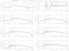 |
Fig. 3. ΔTth, ΔR, and Δaℓ, 0 from ℓ = 1 to ℓmax = 6 for the considered BE-like distortion models. The inset in the top-right panel shows separately the case with the highest value of μ0, which cannot be appreciated in the main panel as it is targeted to much lower values of μ0, in order to appreciate the extremely similar spectral shape of the red and green lines. Except in the top-right panel where ΔR is shown in linear scale, solid lines (or dots) correspond to positive (or negative) values. See also the legend and the text. |
In Fig. 3, ΔR is displayed in the top-right panel. Over the whole frequency range, it is characterised by a module proportional to |μ0| and much smaller than |RBB − 1| even for values of |μ0| not far from FIRAS limits. Again, ΔR depends on frequency. For BE-like distortions, the shape of ΔR is again symmetric with respect to the sign of μ0, with a well-defined maximum (or minimum) located between two minima (or two maxima), clearly defined at lower frequencies and less pronounced at higher frequencies, for μ0 > 0 (or μ0 < 0).
10.4. 21 cm redshifted line
The 21 cm line corresponds to the spin-flip transition in the ground state of neutral hydrogen. This signal is described as the offset of the 21 cm brightness (i.e. antenna) temperature from the background temperature, Tback, along the observed line of sight at a frequency ν that, because of cosmic expansion, is related to the rest frame frequency, ν21 cm = c/(21 cm), by ν = ν21 cm/(1 + z). Tback is usually assumed equal to Tr but, in general, it could include potential distortions and other radiation backgrounds. It depends on the evolution of the gas spin temperature, TS, which represents the excitation temperature of the 21 cm transition, of the fraction of neutral hydrogen, on the Hubble function, H(z), on Ωm, on the matter density contrast, and on the comoving gradient of the line-of-sight component of the comoving velocity (Furlanetto et al. 2006). If TS < Tback (or TS > Tback), the gas is seen in absorption (or in emission). Since the signal detected at a given frequency corresponds to a specific redshift, the 21 cm line provides a tomographic view of the cosmic evolution. A rich set of 21 cm redshifted line models has been studied in Cohen et al. (2017), resulting in an wide envelope of predictions for  .
.
In this work, we consider only the pronounced absorption profile, with an almost symmetric U-shape centred at (78 ± 1) MHz, which was recently found by Bowman et al. (2018) based on an analysis of the data from the Experiment to Detect the Global EoR Signature (EDGES). The absorption feature was found to have an amplitude of  K and a spread of the profile with a full width at half-maximum of
  MHz. These data support the presence of an ionizing background by 180 million years after the Big Bang and a phase of gas heating above the radiation temperature less than 100 million years later (Bowman et al. 2018). The explanation of the 21 cm redshifted line signal found by EDGES might require a substantial cooling of the IGM gas or an additional high-redshift extragalactic radio background, or a combination of them (see e.g., the references at the beginning of Sect. 10.1). The authors provide a suitable analytical representation of the EDGES absorption profile in terms of a flattened Gaussian characterized by a set of best-fit parameters, and we adopt here their expression of
  .
.
The signals considered in Sects. 10.1–10.3, referring to intrinsic CMB spectral distortions, already include the contribution of the unperturbed CMB spectrum. In this section (as well as in Sects. 10.5–10.7), we are considering signals that are superimposed onto the CMB, assumed without spectral distortions, and we then add (in terms of η) the CMB blackbody at the current temperature T0 to  to construct the global signal to be studied as in previous sections.
We compute the coefficients aℓ, 0(ν, β) with the method described in Sect. 3 and, for comparison, also on the basis of Eq. (5), as in Sect. 10.1. The results are shown in Fig. 4.
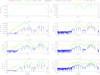 |
Fig. 4. ΔTth, ΔR and Δaℓ, 0 from ℓ = 1 to ℓmax = 6 for the EDGES profile of redshifted 21 cm line (summed in intensity with the CMB blackbody). Solid lines (or dots) correspond to positive (or negative) values. Red and green lines are essentially superimposed at any ℓ. Their difference, multiplied by a factor F to have values compatible with the adopted range, is displayed by the blue lines. Yellow lines refer to the nominal integration error quoted by the routine D01AJF, again multiplied by the factor F. See also the legend and the text. |
We note the consistency between the results based on the integral given by Eq. (5) and our approach: the agreement is excellent up to ℓmax = 6 (the green and red the lines are indistinguishable). Again, their differences are compatible with a combination of higher order terms, that is, beyond ℓ = 6, and integration errors, that are only present in the numerical results. The two types of differences clearly appear, respectively, where the signal is higher and the relative integration error is lower, and where the signal is lower and the relative integration error is higher. The latter point is also evident from the comparison with the nominal integration error quoted by the routine D01AJF. Remarkably, except for the numerical integration uncertainty, the spectral shape of the differences is very similar for all the odd, as well as the even multipoles because they mainly come from the contribution from ℓ = 7 and from ℓ = 8, respectively. In Appendix A, we repeat this analysis adopting a much larger value of β, that implies much larger signals, relatively higher contributions from higher multipoles and relatively lower numerical integration errors: the result clearly supports the above interpretation.
It is interesting to note the complexity, increasing with ℓ, of the features displayed in Fig. 4: they include the alternation of increasing and decreasing behaviours, the number of relative minima and maxima, and the changes of the sign of Δaℓ, 0.
Here, the result for Δa1, 0 corrects the dipole spectrum published in Trombetti & Burigana (2019), expressed there in terms of  (see Eq. (52)), where, for EDGES, the profile
  was accounted in equivalent thermodynamic (not in antenna) temperature. This mere oversight significantly affected only the very small values of
  , making the wings a bit steeper they are.
We note that the frequency, right above 70 MHz, corresponding to the change of sign of Δa1, 0 is shifted at slightly larger values in the case of Δa3, 0 and Δa5, 0, while for the even multipoles it corresponds to a well-defined minimum that falls in the middle of a positive interval of the Δaℓ, 0 profile. The size of this frequency interval decreases as ℓ increases; the same holds, in the case of odd multipoles, for the interval identified by the two signs changes around the above minimum. Also, the increasing with ℓ of the number of sign changes in Δaℓ, 0 implies that, at frequencies outside the above interval, the size of each frequency range with unchanged sign of Δaℓ, 0 decreases with ℓ. These are remarkable features of the considered model.
Remarkably, ΔR (see top-right panel of Fig. 4), again exhibits a frequency dependence related to the assumed intrinsic monopole spectrum: it is positive in the inner frequency range, almost corresponding to the plateau of the absorption feature, and negative in the profile wings. In particular, |ΔR| is comparable to or, typically, greater than |RBB − 1|, across most of the relevant frequency range.
10.5. Extragalactic radio background
An important radio background is produced by extragalactic sources. Differently from most of the signals discussed in previous sections, which are of intrinsically diffuse origin, this background, as well as those discussed in Sects. 10.6 and 10.7, results from the integrated contribution of discrete sources. With galactic surveys able to reach increasingly deeper flux density levels, it is possible to resolve a large fraction of this background. In spite of this, an observationally diffuse residual background comes from faint sources below the survey detection limits. Other than intrinsically interesting, this extragalactic background needs to be accurately known in order to understand the reionization imprints correctly. Remarkably, these classes of signals may also be tightly related. A notable extragalactic radio background is evident in, for example, the radio data by Dowell & Taylor (2018) and it was proposed by Seiffert et al. (2011) to explain the signal excess claimed by ARCADE 2.
We exploit several simple analytical representations of the extragalactic radio background. According to Trombetti & Burigana (2019), we assume the best-fit power-law model,
 (61)
(61)
A careful analysis and prediction of the extragalactic source radio background between 0.151 and 8.44 GHz, also including different source detection thresholds, was carried out by Gervasi et al. (2008a). We consider their best-fit single power-law model for the extragalactic source background signal, multiplied by a factor of 1.3 in order to approximately account for a larger contribution that is, ultimately, likely ascribed to the emerging of star-forming galaxies and radio-quiet active galactic nuclei at fainter flux densities. Indeed, the Lockman Hole Project and deep Low Frequency Array (LOFAR) imaging of the Boötes field support a certain flattening of differential number counts, N′(ν), at 1.4 GHz below ≈100 μJy (Prandoni et al. 2018) and at 0.15 GHz below ≈1 mJy (Retana-Montenegro et al. 2018). This may suggest an increase in N′(ν) of a factor of ∼2 with respect to the estimate of Gervasi et al. (2008a) at the faint flux densities and a ∼30% increase in the extragalactic radio background, which is proportional to  . We then adopt
 (62)
(62)
Gervasi et al. (2008a) provided also an empirical analytical fit function of N′(ν) that can be used to estimate the remaining residual extragalactic radio background when a certain source detection threshold, Smax, is assumed. According to Trombetti & Burigana (2019), we exploit their differential number counts assuming Smax = 50 nJy, which almost corresponds to typical detection limits of the ultra deep reference continuum surveys planned for the Square Kilometre Array (SKA; Prandoni & Seymour 2015). We consider the above factor of ∼2 to be applied to N′(ν) by Gervasi et al. (2008a) at faint flux densities (we then label this case as a ‘High-radio background residual’) and fit the results found in the frequency range considered by the authors to find the corresponding estimate of the remaining residual extragalactic radio background,
 (63)
(63)
with A ≃ 4.7 mK. Different choices of Smax mainly reflects into the value of A.
As in previous section, we add (in terms of η) the CMB blackbody at the current temperature T0 to these radio background models to construct the global signal. The intrinsic monopole spectra are shown in Fig. 5 in terms of ΔTth (top-left panel) with the derived coefficients aℓ, 0(ν, β).
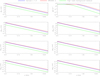 |
Fig. 5. ΔTth, ΔR, and Δaℓ, 0 from ℓ = 1 to ℓmax = 6 for the two considered extragalactic radio background models and an estimate of extragalactic radio source background signal for an assumption of source contribution subtraction (summed in intensity with the CMB blackbody). Solid lines (or dots) correspond to positive (or negative) values. See also the legend and the text. |
The typical power law shapes of the considered intrinsic monopole spectra, after the subtraction of the blackbody at the present temperature T0, are also maintained at higher multipoles and the same holds for their relative amplitudes, as already noted in Trombetti & Burigana (2019) for the dipole.
Again, ΔR exhibits a frequency dependence that is related to the assumed intrinsic monopole spectrum. At low frequencies, below ∼1 GHz, ΔR can have an amplitude comparable to |RBB − 1| or even larger.
10.6. Extragalactic millimetre background
The extragalactic radio source populations that mainly contribute to the radio and to the millimetre background are very different. Whereas steep-spectrum radio sources, particularly at high flux densities, are most important at radio frequencies, extragalactic compact sources with an almost flat, or possibly inverted, spectrum (primarily blazars, flat spectrum radio quasars, and BL Lacertae sources, where are not fully considered in Sect. 10.5) become increasingly relevant at wavelengths shorter than a few centimetres. They can be directly extracted by analyzing CMB maps. The products (Planck Collaboration VII 2013; Planck Collaboration XXVI 2016; Planck Collaboration XLV 2016; Planck Collaboration LIV 2018) from the Planck mission, complemented by the available ground-based data (see e.g., Mocanu et al. 2013) and, in the far-IR, via Herschel (see e.g., López-Caniego et al. 2013) observations, provide crucial information for the characterization of their number counts (De Zotti et al. 2015) (see also De Zotti et al. 2005; Tucci et al. 2011), while a substantial progress at fainter flux densities is expected from the next-generation space missions and deeper multi-frequency ground-based surveys (see e.g., De Zotti et al. 2018, and references therein).
We exploit their differential number counts, N′(ν), including both steep and flat spectrum sources, to estimate the corresponding millimetre background,  , for which we find a power-law approximation, as in Sect. 10.5. We simply extrapolate the power law behaviours of the differential number counts at the lowest available flux density ranges to fainter flux densities. The (currently uncertain) characterization of N′(ν) at much fainter flux densities is relatively less relevant for the estimate of the global background than for the estimate of the residual millimetre background derived given a certain source detection threshold Smax. We consider two assumptions of Smax, namely: (1) 10 mJy (labeled as ‘Intermediate millimetre background residual’), a value that is similar to those typically considered for next-generation space missions; and (2) 100 μJy (labelled as ‘Low millimetre background residual’), representing an estimate of the potential improvement achievable with SKA while considering frequency extrapolation uncertainties from deep radio surveys to millimetre bands.
As expected due to the spectral shapes of the sources that are more relevant at millimetre wavelengths, we find a background spectrum slightly flatter in the millimetre than in the radio, with slopes (of the spectrum expressed in antenna temperature) between ≃ − 2.10 and −2.62, depending on the specific number counts model (with steeper spectra found for the number counts by Tucci et al. 2011) and also on the adopted source detection threshold.
For current numerical estimates we consider, for simplicity, a single slope based on number counts consistent with Planck results from 30 GHz to 857 GHz. We adopt:
 (64)
(64)
with A ≃ 32.4 mK for the millimetre background spectrum and ≃17.3 mK or ≃8.93 mK for residual millimetre background derived for Smax = 10 mJy or Smax = 100 nJy, respectively. We construct the global signal by adding (in terms of η) the CMB blackbody at the current temperature T0.
Our results are shown in Fig. 6. The flattening of ΔTth at ν ∼ 200 GHz and its increasing at higher frequencies are due to the representation in terms of equivalent thermodynamic temperature. We note the different behaviours of Δaℓ, 0 at odd and even multipoles, and the (minimal) increase with ℓ of the frequency where for odd ℓ, the change of sign of Δaℓ, 0 occurs, or for even ℓ, the minimum of Δaℓ, 0 is located.
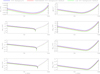 |
Fig. 6. ΔTth, ΔR, and Δaℓ, 0 from ℓ = 1 to ℓmax = 6 for the considered millimetre background model from extragalactic radio sources and estimates of extragalactic source millimetre background signal for two assumptions of source contribution subtraction (summed in intensity with the CMB blackbody). Solid lines (or dots) correspond to positive (or negative) values. See also the legend and the text. |
Figure 6 reports the coefficients aℓ, 0(ν, β) for ℓ = 1, 6, expressed in terms of Δaℓ, 0, derived using the solutions given in Sect. 3. The typical power law shapes of the considered intrinsic monopole spectra, after the subtraction of the blackbody at the present temperature, T0, that are evident in the figure at low frequencies, are kept also at higher multipoles and the same holds for their relative amplitudes, as already noted in Trombetti & Burigana (2019) for the dipole.
ΔR exhibits a dependence on the frequency as well as on the assumed intrinsic monopole spectrum: it is positive and its frequency shape and minimum location are in line with the behaviours of Δaℓ, 0 at even multipoles. On the other hand, the values of |ΔR| are less than |RBB − 1| even at the highest frequencies.
Finally, we note that, despite the fact that the estimate of the extragalactic radio source background in the radio and at millimetre wavelengths, approximated respectively by Eqs. (62) and (64), are based on different models, the results found at ∼20 GHz, a frequency in the middle between the maximum and the minimum frequency of the approximations elaborated in the previous section and in this one, agree within a factor of two or better, as shown by the comparison between Figs. 5 and 6.
10.7. Cosmic infrared background
A precise analysis of CIB spectrum, which is still not well known, can provide a better understanding of the dust-obscured star-formation phase of galaxy evolution.
In spite of its absolute calibration precision of 0.57 mK, the FIRAS characterization of CIB amplitude and shape still presents a substantial uncertainty. According to Fixsen et al. (1998), a suitable analytic representation in terms of photon distribution function of the CIB spectrum at the present time, can be expressed by
 (65)
(65)
where ν0 = c/(100 μm) ≃ 3 THz and xCIB = hν/(kTCIB). The best-fit to FIRAS data gives kF = 0.64 ± 0.12, TCIB = (18.5 ± 1.2) K and I0 = (1.3 ± 0.4) × 10−5 (Fixsen et al. 1998), I0 setting the CIB spectrum amplitude. In the last equality of Eq. (65), x0, CIB = hν0/(kTCIB) ≃ 7.78 (implying xCIB ≃ 7.78 × ν/ν0). The current uncertainty on CIB spectrum amplitude is quite high, with 1σ accuracy of about 30%. Indeed, the direct determination of the CIB spectrum is hard to obtain as it requires absolute intensity measurements and is limited by foreground signals.
We construct the global signal by adding ηCIB with the photon distribution function of the CMB blackbody at the current temperature T0 and consider three simple cases corresponding to the above best-fit and 1σ limits of I0. The results are shown in Fig. 7 in terms of ΔTth, ΔR, and Δaℓ, 0. As shown by the comparison of Fig. 7 with Figs. 1–6 and anticipated in Sect. 10.2, the signal associated to the CIB, strongly increasing with frequency, at ν ≳ 400 GHz dominates over the other extragalactic contributions at any multipole.
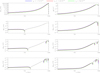 |
Fig. 7. ΔTth, ΔR, and Δaℓ, 0 from ℓ = 1 to ℓmax = 6 for the considered CIB models (summed in intensity with the CMB blackbody). Solid lines (or dots) correspond to positive (or negative) values. See also the legend and the text. |
As has already been found for extragalactic millimetre background, we note the different behaviours of Δaℓ, 0 at odd and even multipoles and, in the frequency range between ≃100 GHz and ≃200 GHz, the increase with ℓ of the frequency where, for odd ℓ, the change of sign of Δaℓ, 0 occurs or, for even ℓ, the shape of Δaℓ, 0 shows a clear steepening. At the highest frequencies, where the power law approximation of the intrinsic monopole spectrum breaks down and the spectrum changes its behaviour approaching its maximum, the shapes of Δaℓ, 0 show remarkable features. They are located at frequencies that decrease as ℓ increases: for example, for ℓ = 2 or 6 they occur at frequencies larger than ∼800 GHz or than ∼500 GHz.
Here, ΔR (top-right panel of Fig. 7) assumes positive values that are much smaller than |RBB − 1| at ν ≲ 400 GHz, but significantly increase with ν at ν ≳ 400 GHz and become comparable to or larger than |RBB − 1| at ν ≳ 700 GHz, achieving a maximum at a frequency ≃800−850 GHz that slightly increases as I0 decreases.
11. Signal combination results
As already states previously in this paper, the method described in Sects. 2–9 and applied in Sect. 10 to specific emissions can be also used to predict the signatures expected from the desired combinations of signals, provided that they are summed in terms of additive quantities. A discussion of the imprints on the dipole spectrum left by combinations of backgrounds associated to cosmological reionization and relevant in the radio can be found in Trombetti & Burigana (2019). Of course, the number of the possible combinations of the models discussed in Sect. 10 is high. Here, we consider a couple of cases that are relevant at millimetre and sub-millimetre wavelengths.
We combine the model of Comptonization plus diffuse FF distortion with the highest values of u and yB with an astrophysical background, namely, the adopted millimetre background model from extragalactic radio sources, an estimate of its residual signal given an assumption of source detection threshold (the ‘Low millimetre background residual’), and the best-fit CIB spectrum. The global signal is constructed by adding the photon distribution functions associated to the considered astrophysical background (Eqs. (64) or (65)) and to the Comptonization plus diffuse FF distortion (Eq. (57)), that already contains the initial unperturbed CMB spectrum, ηi. The results based on the solutions given in Sect. 3 are shown in Figs. 8 and 9 in terms of ΔTth, ΔR, and Δaℓ, 0.
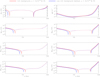 |
Fig. 8. ΔTth, ΔR, and Δaℓ, 0 from ℓ = 1 to ℓmax = 6 for the sum of the considered millimetre background model from extragalactic radio sources or an estimate of its residual signal for an assumption of source detection threshold plus a combined Comptonization and diffuse FF distortion model. Solid lines (or dots) correspond to positive (or negative) values. See also the legend and the text. |
From these figures (see also Figs. 2, 6, and 7), it is possible to appreciate that at the frequencies where a certain component is much stronger than the other, that component also dominates in the combined signal, but this simplification does not hold where the components have comparable amplitudes.
The comparison of Fig. 8 with Figs. 2 and 6 shows that the millimetre background, as well as its residual for the assumed source detection threshold, dominates above a frequency of ∼500 GHz, with only a very little dependence on ℓ. Below a frequency ranging from few tens of GHz to ∼100 GHz the millimetre background and the considered model of Comptonization plus diffuse FF distortion give comparable effects: in particular, the millimetre background and the diffuse FF distortion have also similar power law behaviours (see Eqs. (59) and (64)). As a result, the difference of considering the millimetre background or its residual is more evident in the spectral shapes of their combinations, affecting, respectively, less or more the frequency where the spectra exhibit their sign change, that occurs at frequencies slightly higher than in the case of pure Comptonization plus diffuse FF distortion. The Comptonization distortion is, instead, clearly appreciable at intermediate frequencies, its characteristic plateau appearing in all the Δaℓ, 0.
The comparison of Fig. 9 with Figs. 2 and 7 shows analogous results. The CIB dominates over the Comptonization distortion above a frequency that ranges from ∼100 GHz to ∼200 GHz, slightly increasing with ℓ. Below that frequency, the Comptonization distortion emerges and the combined spectral shapes become flatter. They show also a remarkable change of sign at even ℓ from Figs. 2–6, where Δaℓ, 0 is positive for the CIB and negative for the Comptonization distortion. This does not occur for ΔTth where the contributions from CIB is slightly larger than that from Comptonization, and for ΔR, that is positive in both the cases. At further decreasing frequencies, the FF diffuse emission emerges, and, consequently, the Δaℓ, 0 exhibit, at even and odd ℓ, the typical shapes already found in that case at the lowest frequencies as well as the typical change of sign corresponding to the transition from the range dominated by the FF term to that dominated by the Componization term. The frequency of this transition is only slightly larger than that found in the case of pure Comptonization plus diffuse FF distortion. This frequency shift is significantly smaller than that found above, which combines the Comptonization plus diffuse FF distortion with the millimetre background, because of the smaller additional contribution from the CIB at low frequencies.
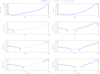 |
Fig. 9. ΔTth, ΔR, and Δaℓ, 0 from ℓ = 1 to ℓmax = 6 for the sum of considered best-fit CIB model plus a combined Comptonization and diffuse FF distortion model. Solid lines (or dots) correspond to positive (or negative) values. See also the legend and the text. |
Of course, the details in the above considerations depend also on the assumed model parameters. We discuss above some cases where the combined contribution from different signals may give not trivial effects. In general, refinements in modelling specific signals and combinations or couplings of them can be included in our method to improve the quality of the results.
12. Maps and angular power spectra
Having evaluated the coefficients aℓ, 0, it suffices then to compute the corresponding maps and angular power spectra. Here, we report just a few examples, also for comparison with the results presented in Burigana et al. (2018), which are based on map generation and inversion performed with the great set of publicly available tools implemented in the Hierarchical Equal Area and isoLatitude Pixelization of the sphere (HEALPix; Górski et al. 2005). Here, we adopt the same pixelization scheme to generate the maps using the aℓ, 0 coefficients: working in real space, based on Eq. (6), we immediately get the map for each multipole component in the reference system with the z axis parallel to the observer velocity. They can be also simply computed in any other reference system (e.g., in Galactic coordinates) given the angle of a pixel direction with respect to the observer velocity direction. Here, we generate the maps with nside = 1024, corresponding to a pixel linear size of ≃3.44 arcmin.
We show the maps for ℓ = 3 and 6 in the case of a BE-like distortion with the maximum value of μ0 (see Sect. 10.3), of a pure Comptonization distortion with the maximum value of u (see Sect. 10.2) and of the best-fit CIB spectrum (see Sect. 10.7). The three adopted frequencies, different for each type of signal, are selected to allow us to make an almost direct comparison with the maps displayed in Burigana et al. (2018) and to appreciate how the method presented here is suitable for a fast map computation, very precise up to the desired order, even where the relevant signal is weak and, in principle, more sensitive to numerical uncertainty. The maps (see Fig. 10) are indeed very clean and without numerical artifacts up to the highest ℓ thanks to the adopted analytical approach; each multipole pattern obviously reflects the corresponding scaling, see Eq. (6), and, in particular, for odd multipoles the maximum and minimum values of each map are equal in module.
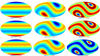 |
Fig. 10. Examples of maps at two specific multipoles in the reference system with the z axis parallel to the observer velocity (left column) and in Galactic coordinates (central and right columns). According to Planck Collaboration I (2020), we adopt l = 264.021° and b = 48.253° for the dipole direction in Galactic coordinates. We display the temperature pattern for a BE-like distortion with μ0 = 1.4 × 10⁻⁵ (top row), a Comptonization distortion with u = 2 × 10⁻⁶ (central row) and the CIB distribution function with best-fit amplitude value I0 = 1.3 × 10⁻⁵ added to the blackbody one (bottom row), minus the temperature pattern coming from the blackbody. The considered frequency and multipole is given above each map. Maps are in equivalent thermodynamic (or CMB) temperature. |
Given the map, we can use publicly available tools, such as the anafast facility of HEALPix, to compute the corresponding angular power spectrum and the aℓ, m coefficients in any reference system (see Goldstein 1984, and also Appendix C, for explicit formulas to transform the aℓ, m under rotation). Indeed, for the considered problem, the aℓ, m with m ≠ 0 do not vanish in reference systems with the z axis not parallel to the observer velocity direction. On the other hand, since the angular power spectrum, Cℓ, is an invariant under rotation of the reference system, we can compute it simply working in the reference system with the z axis parallel to the observer velocity direction, where the aℓ, m with m ≠ 0 vanish, and the coefficients aℓ, 0 are evaluated as in the previous sections
 (66)
(66)
In Fig. 11, we only report the result derived for some of the considered models for ℓ from 1 to 4. We plot the quantity:
![Mathematical equation: $$ \begin{aligned} \frac{\Delta a_{\ell ,0}^2 (\nu ,\beta )}{2\ell +1} = \frac{[a_{\ell ,0}^\mathrm{dist}(\nu ,\beta ) - a_{\ell ,0}^\mathrm{BB}(\beta )]^2}{2\ell +1}\cdot \end{aligned} $$](/articles/aa/full_html/2021/02/aa38845-20/aa38845-20-eq149.gif) (67)
(67)
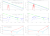 |
Fig. 11. Angular power spectrum of the maps obtained from the difference between the maps produced in the various models and the map obtained for spectrum corresponding to the blackbody at the current temperature T0. See also the legend and the text. |
Equation (67) gives the angular power spectrum of the map obtained from the difference between the map produced in a given model (i.e. for a CMB distorted spectrum or for an astrophysical background spectrum summed with the blackbody spectrum at the current temperature T0) and the map obtained for the blackbody spectrum at the current temperature T0.
There is a good agreement with the results reported by Burigana et al. (2018) – but in the frequency range between 60 and 600 GHz considered for the Cosmic Origins Explorer (COrE) in Fig. 14 (for the CIB) and in Fig. 12 (for BE and Comptonization distortions). As expected, the central panels of Fig. 11, that span from the radio to the sub-millimetre, show that the replacement of the pure BE spectrum with a BE-like spectrum and the inclusion of FF diffuse emission, which is not included in Burigana et al. (2018), is remarkable at lower frequencies (given the high FF model considered here, a little effect is already appreciable at the lowest frequencies of the COrE range, see also Fig. 2).
The signals more relevant at low and high frequencies are displayed in terms of  in the top and bottom panels of Fig. 11, respectively. All the well-defined minima of the various lines displayed in Fig. 11 correspond to the changes of sign of Δaℓ, 0 (see Figs. 2–4 and 6–7), but not in the case of the minimum at ≃80 MHz with respect to the EDGES profile at ℓ = 2 and 4 (appearing in the top panels of Fig. 11, which correspond to the positive minima at the same ℓ’s in Fig. 4).
Finally, we remark that the values of  at the minima corresponding to the sign changes of Δaℓ, 0 (as well as the values of Δaℓ, 0) should, in principle, go to zero at the corresponding frequencies; typically, this does not appear in the plots merely because of their frequency discretization.
13. Varying observer velocity
As discussed in Sect. 1, the observer velocity β = βC + βV(t) is modulated by the time dependent component βV that, in real measurements, mainly comes from the revolution of the Earth or of L2 around the Solar System barycentre (βV ≃ βES ≃ βL2 ≃ 10−4 ≃ 0.081 β). The formalism and the general properties of the solutions presented in previous sections hold for any choice of β. Thus, we can consider a relatively small time interval, Δti, around a certain instant ti, in which the time variation of βV can be neglected and β can be considered as a constant. For example, in a time interval Δti ≃ 1 h, the relative change of β, which is given by Δβ/β ≃ (ΔβV/βV)(βV/β) ≃ ω Δti (βV/β) ≃ 0.0058%, is about one order of magnitude smaller than the current relative uncertainty on βC, given the period of the main modulation P = 2π/ω = 1 yr.
In a time interval, Δti, only a certain fraction of the sky can be observed. The detailed pattern of the sequence of the observed sky positions is defined by the so-called scanning strategy, or observational strategy, which is specific of each considered experiment. Let us define, using  , the all-sky map given by Eq. (6), where β is replaced by βi = β(ti) = βC + βV(ti) and the colatitude θ is replaced by the angle
 ![Mathematical equation: $ \theta^\prime_{\mathrm{i}} = \theta^\prime_{\mathrm{i}}(\boldsymbol{\beta}_{\mathrm{i}},\theta,\phi) = \mathrm{arccos}[({\hat{n}} \cdot \boldsymbol{\beta}_{\mathrm{i}})/\beta_{\mathrm{i}}] $](/articles/aa/full_html/2021/02/aa38845-20/aa38845-20-eq153.gif) between βi and a sky direction corresponding to the unit vector
between βi and a sky direction corresponding to the unit vector  defined by the colatitude θ and the longitude ϕ in any adopted reference system, S. The spherical harmonic coefficients to be used in Eq. (6) are given in Sect. 3 for ℓmax = 6 (or, alternatively, in Sect. 5 for ℓmax = 4 or in Sect. 7 for ℓmax = 2 or 1).
The experiment scanning strategy defines the sequence of pointing maps, Pi(ti, θ, ϕ), on a pixelized sky at the times ti, with i = 1, n and n = τS/Δti where τS is the survey duration: if the direction defined by θ and ϕ is observed in the interval Δti then Pi = 1, otherwise Pi = 0. The averaged map corresponding to a survey based on a set of observer velocities βi is then given by:
 (68)
(68)
where N(θ, ϕ) is the global number of observer velocities βi for which the direction defined by θ and ϕ is observed.
As discussed in Sect. 2, we need to compute the signal in only ℓmax + 1 directions to predict the map up to ℓmax, and the number of signal evaluations required by Eq. (68) is then Nev, ℓmax = (ℓmax + 1) n = (ℓmax + 1) τS/Δti. Of course, the map M(ν, θ, ϕ) can be directly computed through Eqs. (1) and (2) using β = βC + βV(t) at each time, without applying the discretization associated to the choice of the time interval Δti. In this case, since the receiver sampling time, τsamp, is typically much smaller than Δti, the required number of signal evaluations, Nev, d = τS/τsamp, is much larger than Nev, ℓmax. The ratio, rev = Nev, ℓmax/Nev, d, between the required number of signal evaluations in the two cases is rev = τsamp(ℓmax + 1)/Δti ≪ 1. In order to properly compare the computing times in the two approaches, we evaluate this ratio discretizing β = βC + βV(t) according to the choice of Δti also in the direct scheme based on Eqs. (1) and (2). Thus, Nev, d reduces to Nev, d = Ni, pixτS/Δti, where Ni, pix is the number of sky pixels observed in the time interval Δti, and we obtain rev = (ℓmax + 1)/Ni, pix (again, rev ≪ 1).
The method based on Eq. (68) is particularly advantageous when applied to scanning strategies designed for future CMB missions that foresee the use of a huge number of receivers at the focal surface of a wide field of view telescope. The scanning strategies typically foreseen for these missions involve fast spacecraft spin axis precessions, in order to achieve in a short time a large sky coverage and to observe sky pixels with many orientations during the survey to improve the quality of map making results and of polarization analyses (see e.g., Delabrouille et al. 2018; Natoli et al. 2018).
Since  depends on βi, θ and ϕ, Eq. (68) implies that the time varying component βV(t) will introduce in the map M(ν, θ, ϕ) a further modulation along θ and ϕ, which is superimposed onto the main pattern, even if we choose a reference frame S with the z axis parallel to the constant component βC. Although the details of this modulation depend on the experiment scanning strategy, its amplitude amounts to ∼βV/β ∼ 8.1% of the main signal due to the constant velocity component.
For a given model, fixing the other parameters and neglecting the terms in β(ℓ+2) and beyond, the differences of the spherical harmonic coefficients Δaℓ, 0 scale proportionally to βℓ, that is, Δaℓ, 0(β) ≃ Δaℓ, 0(βC) (β/βC)ℓ at the leading order. This property comes from the separation of the system into even and odd multipoles (see Sects. 2–7) and is explicit in the formulas found for the blackbody spectrum (see Sects. 4 and 6). The comparison of the results displayed in Figs. 1 and 4 with those reported in Figs. A.1 and A.2 where the velocity is multiplied by a factor 100 and 10, respectively, also suggests this scaling, providing that the signal is sufficiently smooth in frequency and except for smearing effects where the signal rapidly changes. We verified this property in our numerical results varying β within a ±10% because of the contribution of βV, namely, for realistic deviations of β from βC. This feature can further speed up the computation of  because it allows a fast estimation of the contribution of the time varying component of the velocity over two consecutive multipole patterns, for example, in the case of the dipole and quadrupole, as useful in many applications.
14. Global pattern
In general, the global sky pattern is a combination of intrinsic anisotropies and of the anisotropies induced by the peculiar observer motion. We focus here on the diffuse cosmic signals more relevant in the microwaves, where the intrinsic (mainly of primordial nature) anisotropies are better studied and the background frequency spectrum can be modelled in terms of small deviations from a blackbody.
Working within a reference frame at rest with respect to the background, in a given sky direction identified by θ and ϕ the frequency dependent equivalent thermodynamic temperature can be seen as a function of an effective temperature and of a set of P distortion parameters pj with j = 0, P − 1
 (69)
(69)
Since both fluctuations and distortions are small, TBB(θ, ϕ) ∼ T0 and pj(θ, ϕ) ∼ 0 and we can expand Tth in Taylor’s series around these values. At linear order
 (70)
(70)
where ()0 denotes that the quantities are evaluated at TBB(θ, ϕ) = T0 and pj(θ, ϕ) = 0, that is, for a blackbody with effective temperature T0. Expanding the temperature fluctuation (TBB(θ, ϕ) − T0) and the distortion parameters pj(θ, ϕ) in spherical harmonics with coefficients aBB, ℓ, m and aj, ℓ, m, we have
 (71)
(71)
where aBB, 0, 0Y0, 0 = T0 and  are the average of TBB(θ, ϕ) and pj(θ, ϕ) over the full sky. Although not necessary, we adopt here for simplicity a reference system with the z axis parallel to the observer velocity in order to avoid rotations in the following considerations (see Eq. (84)). In the right-hand side of Eq. (71), the first line represents the (possibly distorted) monopole spectrum, the second line the intrinsic temperature fluctuations, the third line the intrinsic fluctuations of the distortion parameters and (see Eq. (1))
 (72)
(72)
implying that (see Eq. (21)):
 (73)
(73)
and the functions (∂η/∂pj)0 (j = 0, P − 1) depend on the type of distortion. Equation (71) shows that the spectral shape of each distortion term in the monopole spectrum (added to T0) and of the fluctuations of the corresponding distortion parameter is the same, but they are weighted differently depending on the coefficients aj, ℓ, m.
Next, we consider, in the case of distorted spectra, the derivatives ∂η/∂pj and ∂η/∂TBB. In the case of a BE distortion (see Eq. (60)) with a frequency independent chemical potential μ0 (i.e. neglecting for simplicity the spectrum modifications introduced by considering a BE-like distortion that are relevant at lower frequencies), and for small values of μ0, with the approximation ϕBE ≃ (1−1.11μ0)−1/4 we have
 (74)
(74)
 (75)
(75)
implying
![Mathematical equation: $$ \begin{aligned}&\left({ \frac{\partial {\eta }}{\partial {\mu _0}}}\right)_0 \simeq \frac{e^{x} [(1.11/4)x-1]}{(e^{x} -1)^2}, \end{aligned} $$](/articles/aa/full_html/2021/02/aa38845-20/aa38845-20-eq166.gif) (76)
(76)
 (77)
(77)
We derive now ∂η/∂pj and ∂η/∂TBB in the case of a Comptonization distortion with a small Comptonization parameter u and an initial Planckian spectrum, ηi with ϕi ≃ 1 − u (see Eq. (57)), combined with a FF distortion with yB approximated by  with
with ![Mathematical equation: $ {\tilde A}_{\mathrm{FF}} = A_{\mathrm{FF}} [(h/k)\,(\mathrm{GHz}/T_{\mathrm{BB}})]^\zeta \simeq 0.5456 \, A_{\mathrm{FF}} $](/articles/aa/full_html/2021/02/aa38845-20/aa38845-20-eq169.gif) (see Eq. (59)). In principle, also the slope parameter ζ or, for the more general description in Eq. (58), an alternative set of five parameters could be included in the set of distortion parameters pj. For simplicity, we include in the pj only the most relevant emission amplitude parameter in the power law approximation. In the derivatives below, we report only the terms that will not vanish when specified at pj = 0. The terms that are not multiplied by u in ∂η/∂u give
(see Eq. (59)). In principle, also the slope parameter ζ or, for the more general description in Eq. (58), an alternative set of five parameters could be included in the set of distortion parameters pj. For simplicity, we include in the pj only the most relevant emission amplitude parameter in the power law approximation. In the derivatives below, we report only the terms that will not vanish when specified at pj = 0. The terms that are not multiplied by u in ∂η/∂u give
![Mathematical equation: $$ \begin{aligned} \frac{\partial {\eta }}{\partial {u}} =&- \frac{[h\nu /(kT_{\rm BB})]\,e^{h\nu /(kT_{\rm BB})/\phi _{\rm i}}/\phi _{\rm i}^2}{(e^{h\nu /(kT_{\rm BB})/\phi _{\rm i}} - 1)^{2}} \nonumber \\& + {h\nu /(kT_{\rm BB}) / \phi _{\rm i} \, e^{h\nu /(kT_{\rm BB})/\phi _{\rm i}} \over (e^{h\nu /(kT_{\rm BB})/\phi _{\rm i}} - 1)^{2}} \left( {h\nu /(kT_{\rm BB})/\phi _{\rm i} \over { \mathrm{tanh}[h\nu /(kT_{\rm BB})/(2\phi _{\rm i})] }} - 4 \right), \end{aligned} $$](/articles/aa/full_html/2021/02/aa38845-20/aa38845-20-eq170.gif) (78)
(78)
and we get
 (79)
(79)
while
 (80)
(80)
implying
 (81)
(81)
The terms that are not multiplied by u nor by  in ∂η/∂TBB give
 (82)
(82)
implying, again,
 (83)
(83)
Formally, in Eqs. (74), (75), (78), (80), and (82), TBB, μ0, ϕBE(μ0) and ϕi(u) refer to a given sky direction identified by θ and ϕ. However, their relations with θ and ϕ vanish when they are specified for TBB = T0 and pj = 0 as in Eqs. (76), (77), (79), (81), and (83), where indeed x = hν/(kT0).
In general, we have ((∂Tth/∂η)(∂η/∂TBB))0 = 1, as evident also from Eqs. (72), (77), and (83); the coefficients aBB, ℓ, m are then the usual spherical harmonic expansion coefficients defining the CMB temperature anisotropies. Considering both the effects induced by the observer peculiar motion on the monopole and the intrinsic anisotropies, working in the observer reference system with the z axis parallel to the observer velocity, we can combine Eqs. (3) and (71) to derive a global anisotropy pattern
 (84)
(84)
where the coefficients aℓ, m(ν, β) are given in Sect. 3 (or in Sect. 5); we omitted here the first line of the right-hand side of Eq. (71) to obviously avoid a double counting of the monopole that is already included in the term with ℓ = 0 of the last line, where the effect of the observer motion with respect to a frame at rest with the CMB is also taken into account. The focus in this work on the analysis at low multipoles of the effects caused by the observer motion on the isotropic monopole component, neglects the Doppler and aberration effects on the anisotropies, that is, on the first and second lines of the right-hand side of Eq. (84). These effects couple multipoles ℓ to ℓ ± n, particularly in the correlation between ℓ and ℓ ± 1 (Challinor & van Leeuwen 2002; Burles & Rappaport 2006; Kosowsky & Kahniashvili 2011; Amendola et al. 2011; Chluba 2011; Dai & Chluba 2014), a property that has been used to independently constrain β. The effects are indeed more important at high multipoles: their main information comes from ℓ ≳ 100, where many modes can be exploited (Burigana et al. 2018) (see Planck Collaboration LVI 2020 for a recent application to Planck data based on the modulation of the thermal Sunyaev-Zel’dovich effect (Chluba et al. 2005; Notari & Quartin 2016)).
We can rewrite the coefficients aℓ, m(ν, β) as
 (85)
(85)
where  refer to the case of a blackbody spectrum and
  depend on the type of considered distortion.
15. Intrinsic dipole versus kinematic dipole
We focus here on the dipole anisotropy. Including both the effect induced by the observer peculiar motion on the monopole and the intrinsic anisotropies, and using a reference system with the z axis parallel to the observer velocity, the global dipole pattern is characterized by the coefficients:
 (86)
(86)
where
 (87)
(87)
and Δa1, m(ν, β) = 0,  for m ≠ 0. In these equations, the superscript ‘BB’ refers to observer peculiar motion effects while the subscript ‘BB’ refers to intrinsic anisotropies. The coefficients Δa1, 0(ν, β) and
  (through ((∂Tth/∂η)(∂η/∂pj))0), that are related to the type of distortion, do not vanish only in the presence of deviations from a Planckian spectrum.
The typical amplitude of the coefficients Δa1, 0(ν, β) is of the order of  , that is, of ≈βT0, multiplied by the amplitude of the monopole spectral distortion, ΔTth (see the first two left panels from the top in Figs. 2 and 3). The coefficients aj, 1, m characterize the fluctuations of the different types of distortion at ℓ = 1 and then depend significantly on the specific mechanism and not only on the corresponding average distortion parameter and spectral shape. Global spectral distortions are still unobserved, as well their fluctuations (obviously except for the Sunyaev-Zel’dovich effect on galaxy clusters), and it is then reasonable to assume
  .
.
Assuming Gaussian random temperature fluctuations, the coefficients aBB, 1, m are expected to have zero mean and variance given by the angular power spectrum Cℓ at ℓ = 1. Currently, C1 is unknown, but it is typically predicted to be of the order of the temperature anisotropy intrinsic quadrupole C2. Constraining the intrinsic anisotropy power at ℓ = 1 is difficult, but very interesting in the context of future CMB surveys (see Yasini & Pierpaoli 2017 for a method based on the exploitation the leakage of the intrinsic dipole into the CMB monopole and quadrupole and Meerburg et al. 2017 for an analysis based on the observation of the small scale temperature fluctuations that result from gravitational lensing). This topic is related to the power at low multipoles, and in particular, to the low power of the quadrupole discovered by the COBE Differential Microwave Radiometer (DMR; Wright et al. 1996; Hinshaw et al. 1996) and then confirmed by WMAP (Bennett et al. 2013; Hinshaw et al. 2013) and Planck (Planck Collaboration V 2020). Reconstructing the intrinsic anisotropy power at very low multipoles is very important for inflationary models (see Planck Collaboration X 2020 for recent constraints) predicting power suppression at large scales (see e.g., Vilenkin & Ford 1982; Starobinskij 1992; Bridle et al. 2003; Contaldi et al. 2003; Efstathiou 2003; Sinha & Souradeep 2006) and for their connection with universe geometry and topology (see e.g., Linde 1995, 2003; Gratton et al. 2002; Ellis et al. 2002; Lasenby & Doran 2004; Levin 2002).
In general, the amplitudes of the coefficients aBB, 1, m are significantly smaller than the amplitude of the coefficient  , the observed dipole being dominated by the Doppler effect associated to our peculiar motion with respect to the CMB. In the absence of deviations from a Planckian spectrum,
  and Δa1, 0(ν, β) = 0, and any (relatively minor) frequency independent contribution from aBB, 1, 0 is degenerate with
  . The same holds for aBB, 1, m with m ≠ 0 because the sum of dipole terms is still a dipole and, for a Planckian spectrum, it is possible to find a rotation of the reference system that jointly drops the terms with m ≠ 0 at all frequencies (see Appendix C). Thus, the peculiar motion Doppler effect alone does not allow to distinguish the intrinsic dipole from the kinematic dipole, at least in the absence of a very accurate measure of β provided by other methods.
Now, we consider the presence of deviations from a Planckian spectrum. The only frequency dependent terms in Eq. (87) are Δa1, 0(ν, β) and  .
.
Let us assume, as a first simple case (A), that the very large angular scale fluctuations of the spectral distortion parameters are very small in amplitude, namely  . Thus, in the adopted reference system, the only relevant frequency dependence in the dipole pattern is for m = 0 and comes from Δa1, 0(ν, β), while any different choice of the z axis, that is, not parallel (or not antiparallel) to the observer velocity, would imply that the same frequency dependence is polluted in the dipole at m ≠ 0.
In a more general case (B), when we relax the above assumption, that is, for a non-negligible frequency dependent contribution from  , the situation is a bit more complex, but conceptually not so different (in particular for given prescriptions of the coefficients
  ). In the adopted reference system, a frequency dependence related only to the fluctuations of the spectral distortions would appear at m ≠ 0, and the combination of the different frequency dependencies related to the peculiar motion effect and to the fluctuations of the spectral distortions, properly weighted, would appear at m = 0. For a reference system with the z axis not parallel (or not antiparallel) to the observer velocity these frequency dependencies are polluted in the dipole at any m, in a way related to the underlined frequency spectra.
Let us assume that the intrinsic dipole and the kinematic dipole are not aligned (the opposite is possible by chance, but it is very unlikely).
In case (A), one can search for a reference system that drops (or, more realistically, minimize in a statistical sense) the frequency dependence of the coefficients,  for m ≠ 0, implying that its z axis is parallel to β. The components,
  , with m ≠ 0 are then to be ascribed only to the intrinsic temperature fluctuation terms, aBB, 1, m, and although the contribution from aBB, 1, 0 remains hidden in the larger term,
  , the squares of the components,
  , with m ≠ 0, allow us to provide an estimate of the intrinsic dipole angular power spectrum, C1, although with a slightly larger cosmic variance because this estimate is based on only two, instead than three, coefficients. We note that (see Eq. (84)) similar considerations apply in the limit of that approximation, also for ℓ > 1, allowing us to exploit a larger number of modes m. On the other hand, because Δaℓ, m(ν, β) (see Eq. (85)) decreases as βℓ, the information from ℓ > 1 does not add relevant constraints in this scheme.
In case (B), relaxing the assumption  , it is possible to search for a reference system that drops, or minimize, the difference of the frequency dependence of the coefficients,
  , with m ≠ 0, with the behaviour expected from the terms,
  , related to the fluctuations of the distortion parameters (see Eqs. (86) and (87)), added with the intrinsic temperature fluctuation terms, aBB, 1, m. We also note that the frequency dependencies of
  and Δa1, 0(ν, β), although different, are physically connected, being related to the types of involved distortions, and this property can be exploited in the joint analysis of the modes with m = 0 and m ≠ 0, helping, at m ≠ 0, the discrimination between
  and aBB, 1, m.
Therefore, in the presence of spectral distortions, a very careful multifrequency analysis of the dipole pattern, namely, of the frequency behaviour of its spherical harmonic expansion coefficients, can be used, at least in principle, to set constraints on the intrinsic dipole embedded in the kinematic dipole.
We note that the inclusion of the time variation of β (see Sect. 13), although requiring specific implementations, does not conceptually modify the above considerations since it is possible to split the sky area observed in a survey into a proper set of sky areas, each one observed in a shorter time interval and, hence, with a negligible variation of β, without reducing the global statistical information contained in the survey.
16. Discussion and conclusion
The peculiar motion of an observer with respect to the cosmic background in a certain frequency band produces boosting effects in the background anisotropy pattern. In this work, we studied how the frequency spectrum of the background isotropic monopole emission is modified and transferred to the frequency spectra of the patterns at higher multipoles. We performed the analysis in terms of spherical harmonic expansion for various models of background radiation, ranging from the radio to the far-infrared.
Adopting a reference frame with the z axis parallel to the observer motion direction allows us to simplify the problem since it is thanks to this choice that only the spherical harmonic coefficients aℓ, m with m = 0 do not vanish. We derive the system of linear equations to obtain the aℓ, m up to a desired value of ℓmax. For each observational frequency, the aℓ, m are written as linear combinations of the signals at the set of frequencies corresponding to the chosen N = ℓmax + 1 colatitudes θi (Sect. 2). We explicitly write the system and provide the solutions up to ℓmax = 6, as well as for other smaller values of ℓmax. The symmetry property of the associated Legendre polynomials with respect to θ = π/2 is used to separate the system into two subsystems, one for ℓ = 0 and even multipoles and the other for odd multipoles, improving the solutions accuracy with respect to an arbitrary colatitudes choice (Sects. 3–8). We apply these solutions to the case of a blackbody and verify their agreement with the exact analytical solutions for ℓ = 0 and ℓ = 1 at the order in β related to ℓmax (Sects. 4 and 6).
The structure of the solutions is discussed and compared with respect to the general properties of monopole spectrum integration and differentiation (Sect. 9). The coefficients of the solutions can be regarded as sets of weights assigned to a small number of function evaluations, according to adopted order of accuracy, to compute the integrals that define the aℓ, m coefficients. The coefficients of these solutions exhibit remarkable symmetry properties. Some of these properties are the same of the ones shown by the weights used in finite difference formulas to compute numerical derivatives. The implicit mixing of the spectrum derivatives in the solutions is reflected by the absence of that sign alternation property of the weights which appears in finite difference formulas. Indeed, the frequency behaviours of the aℓ, m coefficients are particular sensitive to the local monopole spectrum variation in a way characterized by derivative orders increasing with ℓ.
We applied the method to some models for different types of monopole spectra that can be represented in terms of analytical or semi-analytical functions (Sects. 10 and 11), namely: four types of CMB distorted photon distribution functions, that is, a non-equilibrium imprint at low frequencies, Comptonization, FF, and BE-like distortions; four types of extragalactic background signals, that is, 21 cm redshifted line, radio, and millimetre backgrounds from extragalactic sources, CIB, superimposed onto the CMB Planckian spectrum; some combinations of signal relevant at millimetre and sub-millimetre wavelengths, that is, Comptonization and FF distortions combined with millimetre background from extragalactic sources or with CIB.
For each model, we show the intrinsic monopole spectrum in terms of the difference, ΔTth(ν), between the equivalent thermodynamic temperature for the model and the present CMB temperature T0. Our results are presented in terms of: (i) the difference ΔR(ν, β) = R(ν, β) − RBB(β), where  and RBB(β) are the ratios between the equivalent thermodynamic temperature of observed and intrinsic monopole for the model and for the blackbody at the present temperature T0; (ii) the differences Δaℓ, 0(ν, β) between the spherical harmonic coefficients computed for the model, aℓ, 0(ν, β), and for the blackbody, aℓ, 0(β); we also present (iii) all-sky maps and (iv) angular power spectra (Sect. 12) directly derived from the spherical harmonic coefficients, for some representative cases.
The results are in excellent agreement with those based on more computationally demanding numerical integrations or map generation and inversion (Sects. 10 and 12; see also Appendix A), and even more accurate. The method could be obviously implemented for any ℓmax, however, since β is of the order of 10−3 and the coefficients aℓ, 0(ν, β) scale approximately as βℓ, the solutions presented for ℓmax = 6 allows us to achieve an extremely high accuracy that is sufficient for any application even in the very distant future. We provide also explicit solutions for ℓmax = 4 that are fully adequate for the analysis of forthcoming and proposed surveys. The only accuracy limitation of the proposed scheme derives from neglecting the contributions from higher multipoles, the largest relative errors appearing at ℓmax from ℓmax + 2 and at ℓmax − 1 from ℓmax + 1: the relative errors are very small even at ℓ ≲ ℓmax, while, remarkably, they are fully negligible at the lowest multipoles.
The high number of possible model combinations may result in a variety of signatures in the global signal expected by cosmological plus astrophysical backgrounds. The simplicity and computational efficiency of the proposed method can significantly alleviate the computational effort needed for theoretical predictions and for the comparison with data from future projects for a plethora of cases of interest. These include, for example, signal combinations or possible differences between vectors β that could refer to specific backgrounds or that appear when the observer velocity variation is taken into account (Sect. 13).
We discuss the main features found for the considered background models at the various multipoles in wide frequency ranges. All the patterns at different multipoles are related to the observer peculiar motion, although with a signal amplitude that decreases with ℓ. Thus, they exhibit, both in the whole sky and in different sky regions, spatial correlations at different angular length scales and well-defined geometrical properties, that are related each other, and this would improve their joint analysis that can be optimized considering the observational method and specifications of a given project. As discussed in Trombetti & Burigana (2019) for the dipole in the radio domain, the analysis does not necessarily require the mapping of the entire sky or of a very large fraction of it. Future radio surveys, and in particular the excellent resolution and sensitivity offered by the SKA (Dewdney et al. 2016) for a variety of scientific themes (see e.g., Weltman et al. 2020) can be used to investigate the spectra of the multipoles patterns at low frequencies. In general, the ultra-precise comprehension and subtraction of the Galactic foreground emission is likely to act as the most difficult problem in cosmological analyses at large angular scales.
Finally, we move on to a discussion of the superposition of the CMB intrinsic anisotropies and of the effects induced by the observer peculiar motion focussing on their different frequency behaviours in the presence of CMB spectral distortions (Sect. 14). We find that they can be used, at least in principle, to set constraints on the intrinsic dipole embedded in the kinematic dipole, through a very careful multifrequency analysis of the corresponding spherical harmonic expansion coefficients (Sect. 15; see also Appendix C). Detailed studies, object of future works, can clarify the feasibility of this approach and, possibly, the required specifications.
In general, the above considerations do not strictly rely on the direct absolute determination of the monopole spectrum. Thus, although they come with challenges, these studies can, in principle, be pursued with an anisotropy project, such as the Lite (Light) satellite for the studies of B-mode polarization and Inflation from cosmic background Radiation Detection (LiteBIRD; Matsumura et al. 2014) or a mission like COrE (Delabrouille et al. 2018; de Bernardis et al. 2018) or the Probe of Inflation and Cosmic Origins (PICO; Hanany et al. 2019), provided that an extremely accurate relative and inter-frequency calibration and suppression of systematic effects are achieved (Natoli et al. 2018).
Clearly, the most advantageous observational chance is offered by the next generation of CMB space missions designed to perform ultra-accurate temperature measurements of the whole sky with a highly precise absolute calibration and a relatively high resolution mapping over a wide set of frequencies, as for example, in the Primordial Inflation Explorer (PIXIE; Kogut et al. 2011, 2016), in the Polarized Radiation Imaging and Spectroscopy Mission (PRISM; André et al. 2014), and, as in more recent proposals, to the National Aeronautics and Space Administration (NASA; Chluba et al. 2019a), to the Indian Space Research Organisation (ISRO; CMB Bharat1), and to the European Space Agency (ESA; Delabrouille et al. 2019; Chluba et al. 2019b). These projects have the advantage of measuring the frequency spectrum of the relevant multipole patterns – starting from the monopole.
Acknowledgments
We gratefully acknowledge financial support from the research program RITMARE SP3 WP3 AZ3 U02 and the research contract SMO at CNR/ISMAR, from the INAF PRIN SKA/CTA project FORmation and Evolution of Cosmic STructures (FORECaST) with Future Radio Surveys and from the ASI/Physics Department of the University of Roma–Tor Vergata agreement n. 2016-24-H.0 for study activities of the Italian cosmology community. We gratefully acknowledge the use of the NAG Numerical Library. Some of the results in this paper have been derived using the HEALPix (Górski et al. 2005) package. We also thank the anonymous referee for comments that helped improve the paper.
References
- Amendola, L., Catena, R., Masina, I., et al. 2011, JCAP, 7, 027 [Google Scholar]
- André, P., Baccigalupi, C., Banday, A., et al. 2014, JCAP, 2, 006 [Google Scholar]
- Baiesi, M., Burigana, C., Conti, L., et al. 2020, Phys. Rev. Res., 2, 013210 [Google Scholar]
- Balashev, S. A., Kholupenko, E. E., Chluba, J., Ivanchik, A. V., & Varshalovich, D. A. 2015, ApJ, 810, 131 [NASA ADS] [CrossRef] [Google Scholar]
- Barkana, R. 2018, Nature, 555, 71 [NASA ADS] [CrossRef] [Google Scholar]
- Bennett, C. L., Larson, D., Weiland, J. L., et al. 2013, ApJS, 208, 20 [Google Scholar]
- Bowman, J. D., Rogers, A. E. E., Monsalve, R. A., Mozdzen, T. J., & Mahesh, N. 2018, Nature, 555, 67 [NASA ADS] [CrossRef] [Google Scholar]
- Bridle, S. L., Lewis, A. M., Weller, J., & Efstathiou, G. 2003, MNRAS, 342, L72 [NASA ADS] [CrossRef] [Google Scholar]
- Burigana, C., Danese, L., & De Zotti, G. 1991a, A&A, 246, 49 [Google Scholar]
- Burigana, C., Danese, L., & De Zotti, G. 1991b, ApJ, 379, 1 [NASA ADS] [CrossRef] [Google Scholar]
- Burigana, C., De Zotti, G., & Danese, L. 1995, A&A, 303, 323 [Google Scholar]
- Burigana, C., Popa, L. A., Salvaterra, R., et al. 2008, MNRAS, 385, 404 [NASA ADS] [CrossRef] [Google Scholar]
- Burigana, C., Carvalho, C. S., Trombetti, T., et al. 2018, JCAP, 4, 021 [Google Scholar]
- Burles, S., & Rappaport, S. 2006, ApJ, 641, L1 [NASA ADS] [CrossRef] [Google Scholar]
- Challinor, A., & van Leeuwen, F. 2002, Phys. Rev. D, 65, 103001 [NASA ADS] [CrossRef] [Google Scholar]
- Chluba, J. 2011, MNRAS, 415, 3227 [NASA ADS] [CrossRef] [Google Scholar]
- Chluba, J., & Sunyaev, R. A. 2012, MNRAS, 419, 1294 [NASA ADS] [CrossRef] [Google Scholar]
- Chluba, J., Hütsi, G., & Sunyaev, R. A. 2005, A&A, 434, 811 [NASA ADS] [CrossRef] [EDP Sciences] [Google Scholar]
- Chluba, J., Sazonov, S. Y., & Sunyaev, R. A. 2007, A&A, 468, 785 [NASA ADS] [CrossRef] [EDP Sciences] [Google Scholar]
- Chluba, J., Khatri, R., & Sunyaev, R. A. 2012a, MNRAS, 425, 1129 [Google Scholar]
- Chluba, J., Erickcek, A. L., & Ben-Dayan, I. 2012b, ApJ, 758, 76 [Google Scholar]
- Chluba, J., Kogut, A., Patil, S. P., et al. 2019a, BAAS, 51, 184 [Google Scholar]
- Chluba, J., Abitbol, M. H., Aghanim, N., et al. 2019b, ArXiv e-prints [arXiv:1909.01593] [Google Scholar]
- Chluba, J., Ravenni, A., & Bolliet, B. 2020a, MNRAS, 492, 177 [Google Scholar]
- Chluba, J., Ravenni, A., & Acharya, S. K. 2020b, MNRAS, 498, 959 [Google Scholar]
- Cohen, A., Fialkov, A., Barkana, R., & Lotem, M. 2017, MNRAS, 472, 1915 [NASA ADS] [CrossRef] [Google Scholar]
- Contaldi, C. R., Peloso, M., Kofman, L., & Linde, A. 2003, JCAP, 2003, 002 [Google Scholar]
- Cooray, A., & Furlanetto, S. R. 2004, ApJ, 606, L5 [Google Scholar]
- Dai, L., & Chluba, J. 2014, Phys. Rev. D, 89, 123504 [Google Scholar]
- Danese, L., & Burigana, C. 1994, Lect. Notes Phys., 429, 28 [Google Scholar]
- Danese, L., & De Zotti, G. 1980, A&A, 84, 364 [Google Scholar]
- Danese, L., & De Zotti, G. 1981, A&A, 94, L33 [Google Scholar]
- de Bernardis, P., Ade, P. A. R., Baselmans, J. J. A., et al. 2018, JCAP, 4, 015 [Google Scholar]
- De Zotti, G., Ricci, R., Mesa, D., et al. 2005, A&A, 431, 893 [NASA ADS] [CrossRef] [EDP Sciences] [Google Scholar]
- De Zotti, G., Castex, G., González-Nuevo, J., et al. 2015, JCAP, 2015, 018 [NASA ADS] [CrossRef] [Google Scholar]
- De Zotti, G., Negrello, M., Castex, G., Lapi, A., & Bonato, M. 2016, JCAP, 3, 047 [Google Scholar]
- De Zotti, G., González-Nuevo, J., Lopez-Caniego, M., et al. 2018, JCAP, 4, 020 [Google Scholar]
- Delabrouille, J., de Bernardis, P., Bouchet, F. R., et al. 2018, JCAP, 4, 014 [Google Scholar]
- Delabrouille, J., Abitbol, M. H., Aghanim, N., et al. 2019, ArXiv e-prints [arXiv:1909.01591] [Google Scholar]
- Deshpande, A. A. 2018, ApJ, 866, L7 [NASA ADS] [CrossRef] [Google Scholar]
- Dewdney, P., Turner, W., Braun, R., et al. 2016, SKA1 System Baseline Design, Square Kilometre Array Organisation (UK: Jodrell Bank) [Google Scholar]
- Dowell, J., & Taylor, G. B. 2018, ApJ, 858, L9 [NASA ADS] [CrossRef] [Google Scholar]
- Efstathiou, G. 2003, MNRAS, 343, L95 [Google Scholar]
- Ellis, G. F. R., McEwan, P., Stoeger, W., & Dunsby, P. 2002, Gen. Rel. Grav., 34, 1461 [Google Scholar]
- Ewall-Wice, A., Chang, T.-C., Lazio, J., et al. 2018, ApJ, 868, 63 [NASA ADS] [CrossRef] [Google Scholar]
- Fixsen, D. J. 2009, ApJ, 707, 916 [Google Scholar]
- Fixsen, D. J., Cheng, E. S., Gales, J. M., et al. 1996, ApJ, 473, 576 [NASA ADS] [CrossRef] [Google Scholar]
- Fixsen, D. J., Dwek, E., Mather, J. C., Bennett, C. L., & Shafer, R. A. 1998, ApJ, 508, 123 [NASA ADS] [CrossRef] [Google Scholar]
- Forman, M. A. 1970, Planet. Space Sci., 18, 25 [NASA ADS] [CrossRef] [Google Scholar]
- Fornberg, B. 1988, Math. Comput., 51, 699 [Google Scholar]
- Fornberg, B. 1998, SIAM Rev., 40, 685 [Google Scholar]
- Furlanetto, S. R., Oh, S. P., & Briggs, F. H. 2006, Phys. Rep., 433, 181 [NASA ADS] [CrossRef] [Google Scholar]
- Gervasi, M., Tartari, A., Zannoni, M., Boella, G., & Sironi, G. 2008a, ApJ, 682, 223 [NASA ADS] [CrossRef] [Google Scholar]
- Gervasi, M., Zannoni, M., Tartari, A., Boella, G., & Sironi, G. 2008b, ApJ, 688, 24 [NASA ADS] [CrossRef] [Google Scholar]
- Gnedin, N. Y. 2000, ApJ, 542, 535 [NASA ADS] [CrossRef] [Google Scholar]
- Goldstein, J. D. 1984, J. Geophys. Res., 89, 4413 [Google Scholar]
- Górski, K. M., Hivon, E., Banday, A. J., et al. 2005, ApJ, 622, 759 [NASA ADS] [CrossRef] [Google Scholar]
- Gould, R. J. 1984, ApJ, 285, 275 [NASA ADS] [CrossRef] [Google Scholar]
- Gratton, S., Lewis, A., & Turok, N. 2002, Phys. Rev. D, 65, 043513 [NASA ADS] [CrossRef] [Google Scholar]
- Hanany, S., Alvarez, M., Artis, E., et al. 2019, BAAS, 51, 194 [Google Scholar]
- Hills, R., Kulkarni, G., Meerburg, P. D., & Puchwein, E. 2018, Nature, 564, E32 [CrossRef] [Google Scholar]
- Hinshaw, G., Branday, A. J., Bennett, C. L., et al. 1996, ApJ, 464, L25 [NASA ADS] [CrossRef] [Google Scholar]
- Hinshaw, G., Larson, D., Komatsu, E., et al. 2013, ApJS, 208, 19 [Google Scholar]
- Hu, W., Scott, D., & Silk, J. 1994, ApJ, 430, L5 [NASA ADS] [CrossRef] [Google Scholar]
- Illarionov, A. F., & Sunyaev, R. A. 1974, AZh, 51, 1162 [Google Scholar]
- Itoh, N., Sakamoto, T., Kusano, S., Nozawa, S., & Kohyama, Y. 2000, ApJS, 128, 125 [NASA ADS] [CrossRef] [Google Scholar]
- Karzas, W. J., & Latter, R. 1961, ApJS, 6, 167 [NASA ADS] [CrossRef] [Google Scholar]
- Kogut, A., Fixsen, D. J., Chuss, D. T., et al. 2011, JCAP, 7, 025 [Google Scholar]
- Kogut, A., Chluba, J., Fixsen, D. J., Meyer, S., & Spergel, D. 2016, Proc. SPIE, 9904, 99040W [Google Scholar]
- Kompaneets, A. S. 1957, Sov. J. Exp. Theor. Phys., 4, 730 [Google Scholar]
- Kosowsky, A., & Kahniashvili, T. 2011, Phys. Rev. Lett., 106, 191301 [Google Scholar]
- Lasenby, A., & Doran, C. 2004, AIP Conf. Ser., 736, 53 [Google Scholar]
- Levin, J. 2002, Phys. Rep., 365, 251 [NASA ADS] [CrossRef] [Google Scholar]
- Lightman, A. P. 1981, ApJ, 244, 392 [NASA ADS] [CrossRef] [Google Scholar]
- Linde, A. 1995, Phys. Lett. B, 351, 99 [NASA ADS] [CrossRef] [Google Scholar]
- Linde, A. 2003, JCAP, 2003, 002 [Google Scholar]
- López-Caniego, M., González-Nuevo, J., Massardi, M., et al. 2013, MNRAS, 430, 1566 [NASA ADS] [CrossRef] [Google Scholar]
- Lucca, M., Schöneberg, N., Hooper, D. C., Lesgourgues, J., & Chluba, J. 2020, JCAP, 2020, 026 [Google Scholar]
- Matsumura, T., Akiba, Y., Borrill, J., et al. 2014, J. Low Temp. Phys., 176, 733 [NASA ADS] [CrossRef] [Google Scholar]
- Meerburg, P. D., Meyers, J., & van Engelen, A. 2017, Phys. Rev. D, 96, 083519 [Google Scholar]
- Mirabel, I. F. 2019, IAU Symp., 346, 365 [Google Scholar]
- Mocanu, L. M., Crawford, T. M., Vieira, J. D., et al. 2013, ApJ, 779, 61 [NASA ADS] [CrossRef] [Google Scholar]
- Muñoz, J. B., & Loeb, A. 2018, Nature, 557, 684 [NASA ADS] [CrossRef] [Google Scholar]
- Natoli, P., Ashdown, M., Banerji, R., et al. 2018, JCAP, 4, 022 [Google Scholar]
- Nordberg, H. P., & Smoot, G. F. 1998, ArXiv e-prints [arXiv:astro-ph/9805123] [Google Scholar]
- Notari, A., & Quartin, M. 2016, Phys. Rev. D, 94, 043006 [Google Scholar]
- Oh, S. P. 1999, ApJ, 527, 16 [NASA ADS] [CrossRef] [Google Scholar]
- Peyraud, J. 1968, J. Phys. France, 29, 306 [EDP Sciences] [Google Scholar]
- Planck Collaboration VII. 2013, A&A, 550, A133 [NASA ADS] [CrossRef] [EDP Sciences] [Google Scholar]
- Planck Collaboration I. 2016, A&A, 594, A1 [NASA ADS] [CrossRef] [EDP Sciences] [Google Scholar]
- Planck Collaboration V. 2016, A&A, 594, A5 [NASA ADS] [CrossRef] [EDP Sciences] [Google Scholar]
- Planck Collaboration VIII. 2016, A&A, 594, A8 [NASA ADS] [CrossRef] [EDP Sciences] [Google Scholar]
- Planck Collaboration XXVI. 2016, A&A, 594, A26 [NASA ADS] [CrossRef] [EDP Sciences] [Google Scholar]
- Planck Collaboration XLV. 2016, A&A, 596, A106 [NASA ADS] [CrossRef] [EDP Sciences] [Google Scholar]
- Planck Collaboration LIV. 2018, A&A, 619, A94 [NASA ADS] [CrossRef] [EDP Sciences] [Google Scholar]
- Planck Collaboration I. 2020, A&A, 641, A1 [CrossRef] [EDP Sciences] [Google Scholar]
- Planck Collaboration II. 2020, A&A, 641, A2 [CrossRef] [EDP Sciences] [Google Scholar]
- Planck Collaboration III. 2020, A&A, 641, A3 [NASA ADS] [CrossRef] [EDP Sciences] [Google Scholar]
- Planck Collaboration V. 2020, A&A, 641, A5 [CrossRef] [EDP Sciences] [Google Scholar]
- Planck Collaboration VI. 2020, A&A, 641, A6 [NASA ADS] [CrossRef] [EDP Sciences] [Google Scholar]
- Planck Collaboration X. 2020, A&A, 641, A10 [CrossRef] [EDP Sciences] [Google Scholar]
- Planck Collaboration LVI. 2020, A&A, 644, A100 [EDP Sciences] [Google Scholar]
- Ponente, P. P., Diego, J. M., Sheth, R. K., et al. 2011, MNRAS, 410, 2353 [NASA ADS] [CrossRef] [Google Scholar]
- Prandoni, I., & Seymour, N. 2015, Advancing Astrophysics with the Square Kilometre Array (AASKA14), 67 [CrossRef] [Google Scholar]
- Prandoni, I., Guglielmino, G., Morganti, R., et al. 2018, MNRAS, 481, 4548 [NASA ADS] [CrossRef] [Google Scholar]
- Press, W. 1992, Numerical Recipes in FORTRAN: The Art of Scientific Computing (Cambridge: Cambridge University Press) [Google Scholar]
- Ravenni, A., & Chluba, J. 2020, JCAP, 10, 025 [Google Scholar]
- Retana-Montenegro, E., Röttgering, H. J. A., Shimwell, T. W., et al. 2018, A&A, 620, A74 [NASA ADS] [CrossRef] [EDP Sciences] [Google Scholar]
- Rybicki, G., & Lightman, A. 2008, Radiative Processes in Astrophysics, Physics Textbook (New York: Wiley) [Google Scholar]
- Salvaterra, R., & Burigana, C. 2002, MNRAS, 336, 592 [NASA ADS] [CrossRef] [Google Scholar]
- Seiffert, M., Fixsen, D. J., Kogut, A., et al. 2011, ApJ, 734, 6 [NASA ADS] [CrossRef] [Google Scholar]
- Sharma, P. 2018, MNRAS, 481, L6 [NASA ADS] [CrossRef] [Google Scholar]
- Singal, J., Fixsen, D. J., Kogut, A., et al. 2011, ApJ, 730, 138 [NASA ADS] [CrossRef] [Google Scholar]
- Sinha, R., & Souradeep, T. 2006, Phys. Rev. D, 74, 043518 [NASA ADS] [CrossRef] [Google Scholar]
- Slosar, A. 2017, Phys. Rev. Lett., 118, 151301 [NASA ADS] [CrossRef] [Google Scholar]
- Starobinskij, A. A. 1992, Sov. J. Exp. Theor. Phys. Lett., 55, 489 [Google Scholar]
- Stebbins, A., & Silk, J. 1986, ApJ, 300, 1 [Google Scholar]
- Subrahmanyan, R., & Cowsik, R. 2013, ApJ, 776, 42 [NASA ADS] [CrossRef] [Google Scholar]
- Sunyaev, R. A., & Khatri, R. 2013, Int. J. Mod. Phys. D, 22, 1330014 [Google Scholar]
- Sunyaev, R. A., & Zel’dovich, Y. B. 1970, Ap&SS, 7, 20 [Google Scholar]
- Thorne, K. S. 1981, MNRAS, 194, 439 [NASA ADS] [Google Scholar]
- Trombetti, T., & Burigana, C. 2014, MNRAS, 437, 2507 [NASA ADS] [CrossRef] [Google Scholar]
- Trombetti, T., & Burigana, C. 2019, A&A, 631, A61 [EDP Sciences] [Google Scholar]
- Tucci, M., Toffolatti, L., De Zotti, G., & Martínez-González, E. 2011, A&A, 533, A57 [NASA ADS] [CrossRef] [EDP Sciences] [Google Scholar]
- Vilenkin, A., & Ford, L. H. 1982, Phys. Rev. D, 26, 1231 [CrossRef] [MathSciNet] [Google Scholar]
- Weltman, A., Bull, P., Camera, S., et al. 2020, PASA, 37, e002 [CrossRef] [Google Scholar]
- Wright, E. L., Bennett, C. L., Gorski, K., Hinshaw, G., & Smoot, G. F. 1996, ApJ, 464, L21 [NASA ADS] [CrossRef] [Google Scholar]
- Yasini, S., & Pierpaoli, E. 2017, Phys. Rev. Lett., 119, 221102 [Google Scholar]
- Zel’dovich, Y. B., & Levich, E. V. 1969, Sov. J. Exp. Theor. Phys., 28, 1287 [Google Scholar]
- Zel’dovich, Y. B., Illarionov, A. F., & Sunyaev, R. A. 1972, Sov. J. Exp. Theor. Phys., 35, 643 [NASA ADS] [Google Scholar]
Appendix A: Numerical tests with amplified observer velocity
In Sects. 10.1 and 10.4, we compare, for two very different cases, the results based on the solutions described in Sect. 3 and on a direct numerical integration (see Eq. (5)) to find differences that are compatible with a combination of higher order terms, that is, beyond ℓ = 6, and integration errors, the latter becoming more relevant at increasing ℓ and decreasing signals, in connection with the low value of the observer velocity, β.
To better clarify this aspect, we perform the same type of comparison, but adopting a much larger value of β, in order to exploit much larger signals and relatively higher contributions from higher multipoles and to deal with relatively lower numerical integration errors. Here, we reconsider the cases of the non-equilibrium model and of the EDGES profile of redshifted 21 cm line, but assuming a value of β arbitrarily amplified respectively by a factor 100 and 10, this choice being motivated by their different signal amplitudes in their relevant frequency ranges.
We report the results for Δaℓ, 0 found using the equations in Sect. 3 and the Eq. (5) for ℓ = 1, 6, as well as the results based on Eq. (5) for ℓ = 7 and 8. They are shown in Figs. A.1 and A.2. As expected, and as evident from the figures, such higher values of β imply a strong reduction of the relative numerical integration error, making feasible an accurate computation of Δaℓ, 0 at larger ℓ. Thus, the differences at ℓ = 1, 6 between the results found with the two methods come essentially only from higher order terms, neglected in the equations of Sect. 3, that are obviously dominated by the contributions from ℓ = 7 at odd multipoles and from ℓ = 8 at even multipoles.
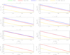 |
Fig. A.1. Δaℓ, 0 for the considered non-equilibrium model (ν0 ≃ 0.35 GHz and α ≃ 3.36), assuming a value of β multiplied by a factor 100; ℓ ranges from 1 to ℓmax = 6 in the case of the solutions described in Sect. 3 and up to 8 in the case of numerical integration (with the routine D01AJF) based on Eq. (5). Solid lines (or dots) correspond to positive (or negative) values. Green and red lines are essentially superimposed up to ℓ = 6. Their difference, multiplied by a factor F to have values compatible with the adopted range, is displayed by the blue lines. Yellow lines refer to the nominal integration error quoted by the routine D01AJF, again multiplied by the factor F. See also the legend and the text. |
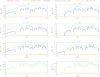 |
Fig. A.2. Same as in Fig. A.1, but for the EDGES profile of redshifted 21 cm line (summed in intensity with the CMB blackbody) and assuming a value of β multiplied by a factor 10. See also the legend and the text. |
We note that the order of magnitude of Δa7, 0 (or of Δa8, 0) is equal to the order of magnitude of the differences between the results found with the two methods at odd (or even) multipoles. The spectral shapes of Δaℓ, 0 in the case of the non-equilibrium model are featureless, reflecting the original power law shape of the monopole spectrum when expressed in terms of ΔTth. Conversely, the spectral shapes of Δaℓ, 0 in the case of the EDGES profile are rich in features, increasing in number at increasing ℓ. Remarkably, the spectral shape of the differences between the results found with the two methods reflects the spectral shape of Δa7, 0 (or of Δa8, 0) at odd (or even) multipole.
As discussed in Sect. 2, the above properties derive from the separation of the system in two subsystems, one at odd ℓ the other at even ℓ, associated to the adoption of a set of colatitudes symmetric with respect to π/2 (plus π/2). This suppresses in each aℓ, 0 at odd (or even) ℓ the contribution of the multipole immediately larger than maximum odd (or even) multipole considered in the system solution (see also, for comparison, the discussion in Sect. 7). This is particularly important in practice for the ‘robustness’ of the accuracy of the solutions presented in this work, suitable for the real (low) value of β, and especially in the case of spectra rich in features for which changes of sign of Δaℓ, 0 and extremely low values of Δaℓ, 0 may occur at different frequencies for different ℓ, possibly enhancing the relative contribution of the missing higher order terms.
Appendix B: Double Compton Gaunt factor
As anticipated in Sect. 10.3, here we provide an improved approximation for the double Compton Gaunt factor (see also Ravenni & Chluba 2020; Chluba et al. 2020b for recent studies) in the elastic limit, suitable for small BE-like distortions. Writing the double Compton term according to Burigana et al. (1995), and accounting separately in the rate for the correction factor, Cmr, for mildly relativistic thermal plasma in the soft photon limit (Chluba et al. 2007), the double Compton Gaunt factor can be written as (Burigana et al. 1991a)
![Mathematical equation: $$ \begin{aligned} g_{\rm DC} (x_{\rm e}) = \frac{ \int _{2x_{\rm e}}^\infty x^{\prime 4}_{\rm e} \, [1+\eta (x^{\prime }_{\rm e} - x_{\rm e})] \, \eta (x^{\prime }_{\rm e}) \, \left[{ { w} { F({ w}) \over 2 } }\right] \, \mathrm{d}x^{\prime }_{\rm e} }{ \int _0^\infty [1+\eta (x^{\prime }_{\rm e})] \, \eta (x^{\prime }_{\rm e}) \, x^{\prime 4}_{\rm e} \mathrm{d}x^{\prime }_{\rm e} }, \end{aligned} $$](/articles/aa/full_html/2021/02/aa38845-20/aa38845-20-eq204.gif) (B.1)
(B.1)
where
![Mathematical equation: $$ \begin{aligned} { w} { F({ w}) \over 2 } =&\frac{1}{2} (1-{ w})\\& \times \left[ { 1 + (1-{ w})^2 + \frac{{ w}^2(1+{ w}^2)}{(1-{ w})^2} + { w}^4 +{ w}^2(1-{ w})^2 } \right], \nonumber \end{aligned} $$](/articles/aa/full_html/2021/02/aa38845-20/aa38845-20-eq205.gif) (B.2)
(B.2)
with w the ratio between the frequencies of the created and incident photons, 0 ≤ w ≤ 1/2 and wF(w)/2 → 1 as w → 1 (Gould 1984). For a (pure) BE spectrum with a frequency independent chemical potential μ and equilibrium temperature ![Mathematical equation: $ T_{\rm BE} = T_{\rm eq} = [h/(4k)] \int_0^\infty (1+\eta) \eta \nu^4 {\rm d}\nu/\int_0^\infty \eta \nu^3 {\rm d}\nu $](/articles/aa/full_html/2021/02/aa38845-20/aa38845-20-eq206.gif) (Peyraud 1968; Zel’dovich & Levich 1969), the integral at denominator in Eq. (B.1) is simply 4I3f(μ), with
(Peyraud 1968; Zel’dovich & Levich 1969), the integral at denominator in Eq. (B.1) is simply 4I3f(μ), with  , I3 = π4/15 and f(μ)→1 in the Planckian limit μ → 0. Thus, for a pure BE spectrum only the integral at numerator of Eq. (B.1) needs a numerical computation. We have performed this calculation using both a Gaussian quadrature scheme (Press 1992) and the NAG routine D01AJF, adopting a very large upper integration limit (set to 500, to have a good estimation also at very high frequencies) and working with a dimensionless frequency in logarithmic space as integration variable. We first consider the case of a blackbody spectrum and compare the results of two methods (see Fig. B.1): clearly, they are in excellent agreement. We then consider the case of a (pure) BE spectrum with μ0 = 1.4 × 10⁻⁵, the largest value considered in this work. The relative differences between gDC computed for this case and in the case of a blackbody spectrum are less than few ×10−2% in the whole frequency range, and obviously it decreases for decreasing values of μ0. Although the very low frequencies give only a little relative contribution to the integral, a similar comparison for a BE-like spectrum is in principle a bit more difficult, because the spectrum at low frequencies depends also on gDC. On the other hand, the above difference represents a good upper limit estimation also when applied to a BE-like spectrum with the same high frequency asymptotic value of μ0, because a BE-like spectrum differs from the blackbody less than a pure BE spectrum.
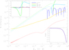 |
Fig. B.1. Comparison between the results of various approximations and accurate numerical integrations of Eq. (B.1). The bottom-right inset gives the numerical result derived with the NAG routine D01AJF with a relative accuracy of 10−12 in the case of the blackbody spectrum. The main plot reports the per cent difference of various estimations of Eq. (B.1) with respect to the NAG D01AJF result for the blackbody spectrum: the approximation presented here (Current, see Eq. (B.5)); the NAG D01AJF result but for a pure BE spectrum with μ0 = 1.4 × 10⁻⁵ (BE); the approximations reported in Burigana et al. (1991a) (BB-BDD, see Eq. (B.3)) and in Chluba & Sunyaev (2012) (BB-CS, see Eq. (B.4)); the numerical result derived with a Gaussian quadrature scheme (Press 1992) with the accuracy parameter (EPS) set to 10−9 and 2048 points in the case of the blackbody spectrum. Solid lines (or dots) correspond to positive (or negative) values. The top-left inset displays the same results of the main plot, but in a restricted frequency range and with a linear scale on the y-axis. See also the legend and the text. |
An approximation for gDC(xe) which, as explicitly stated by the authors, works well only at low frequencies, where the rate is higher, was found by Burigana et al. (1991a)
 (B.3)
(B.3)
Of course, for very small distortions xe ≃ x. In the limit μ ≪ 1, Chluba & Sunyaev (2012) found the approximation
![Mathematical equation: $$ \begin{aligned} {\hat{g}}_{\rm DC} (x) \simeq &e^{ -2x}\\&\times [1+ (3/2) x + (29/24) x^2 + (11/16) x^3 + (5/12) x^4].\nonumber \end{aligned} $$](/articles/aa/full_html/2021/02/aa38845-20/aa38845-20-eq209.gif) (B.4)
(B.4)
Figure B.1 shows the relative accuracies of these two formulas. The latter works significantly better than the former at x ≳ 0.3, providing a little improvement at smaller frequencies (the two approximations clearly agree to first order in Taylor’s series for small x). On the other hand, an error at some % level still remains when using Eq. (B.4) at x > 1.
We then search for a better description of the numerical result. Considering the very good accuracy of Eq. (B.4) at low frequencies, we consider the following expression:
![Mathematical equation: $$ \begin{aligned} g_{\rm DC} (x) \simeq \,\, {\hat{g}}_{\rm DC} (x) \, 10^{P(X)} \, e^{-({\hat{x}}/x)^m} + {\hat{g}}_{\rm DC} (x) [1 - e^{-({\hat{x}}/x)^m}], \end{aligned} $$](/articles/aa/full_html/2021/02/aa38845-20/aa38845-20-eq210.gif) (B.5)
(B.5)
where X = log10x, P(X) is a polynomial of a certain degree d,  and m are a dimensionless frequency and an exponent. P(X) modifies the approximation represented by
  to better describe the numerical results at high frequencies, while
  and m define the exponential weights to assure a smooth transition from low to high frequencies, around
  . We fit our numerical results (for instance, the ones derived with the D01AJF routine) for gDC(x) in the Planckian limit to find the values of
  , m, d, varying them on a simple three dimensional grid, and of the best-fit polynomial coefficients. We find m = 1.6,
  , d = 17 and the following polynomial coefficients, from the power of order 0 to the power of order d:
The accuracy of this approximation is also displayed in Fig. B.1: it is always better than ≃1% and better than ≃0.1−0.2% in the whole relevant frequency range.
Appendix C: Reference system rotation and dipole terms with m≠ 0
Let us consider a real field, T(θ, ϕ), defined by the spherical harmonics coefficients Aℓ, m in a given reference system, S, with polar coordinates θ and ϕ, that is:
 (C.1)
(C.1)
and another reference system S′, with coordinates θ′ and ϕ′, that is defined, with respect to S, by the Euler angles αE, βE, γE. The range of αE and γE is defined modulo 2π radians: we adopt the range [0, 2π] (but another widely adopted choice is, for example, [ − π, π]). The range of βE covers π radians: we adopt the range [0, π] (but it could be, for example, [ − π/2, π/2]). In the reference system S′
 (C.2)
(C.2)
where Dℓ, j are the corresponding (rotated) spherical harmonics coefficients. According to Goldstein (1984)
 (C.3)
(C.3)
where
 (C.4)
(C.4)
here i2 = −1 and  are the Jacobi polynomials
 (C.5)
(C.5)
expressed in explicit polynomial form. For r = 0, we simply have  .
.
Defining A1, 0 = a1, 0, A1, 1 = b1, 1 + i c1, 1 (and, for symmetry, A1, −1 = −b1, 1 + i c1, 1), after some algebra one gets
![Mathematical equation: $$ \begin{aligned}&\mathrm{Re} (D_{1,1}) = \frac{\sqrt{2}}{2} \, a_{1,0} \, \mathrm{sin} \, \beta _{\rm E} \, \mathrm{sin} \, \gamma _{\rm E} \\&\qquad \qquad \quad + \frac{1+\mathrm{cos} \, \beta _{\rm E}}{2} \, [ b_{1,1} \, \mathrm{cos} \, (\alpha _{\rm E} + \gamma _{\rm E}) - c_{1,1} \, \mathrm{sin} \, (\alpha _{\rm E} + \gamma _{\rm E}) ] \nonumber \\&\qquad \qquad \quad + \frac{1-\mathrm{cos} \, \beta _{\rm E}}{2} \, [ b_{1,1} \, \mathrm{cos} \, (\alpha _{\rm E} - \gamma _{\rm E}) - c_{1,1} \mathrm{sin} \, (\alpha _{\rm E} - \gamma _{\rm E}) ] \nonumber , \end{aligned} $$](/articles/aa/full_html/2021/02/aa38845-20/aa38845-20-eq225.gif) (C.6)
(C.6)
![Mathematical equation: $$ \begin{aligned}&\mathrm{Im} (D_{1,1}) = - \frac{\sqrt{2}}{2} \, a_{1,0} \, \mathrm{sin} \, \beta _{\rm E} \, \mathrm{cos} \, \gamma _{\rm E} \\&\qquad \qquad \quad + \frac{1+\mathrm{cos} \, \beta _{\rm E}}{2} \, [ b_{1,1} \, \mathrm{sin} \, (\alpha _{\rm E} + \gamma _{\rm E}) + c_{1,1} \, \mathrm{cos} \, (\alpha _{\rm E} + \gamma _{\rm E}) ] \nonumber \\&\qquad \qquad \quad - \frac{1-\mathrm{cos} \, \beta _{\rm E}}{2} \, [ b_{1,1} \, \mathrm{sin} \, (\alpha _{\rm E} - \gamma _{\rm E}) + c_{1,1} \, \mathrm{cos} \, (\alpha _{\rm E} - \gamma _{\rm E}) ]. \nonumber \end{aligned} $$](/articles/aa/full_html/2021/02/aa38845-20/aa38845-20-eq226.gif) (C.7)
(C.7)
A rotation of the reference system S → S′, that is, a set of Euler angles αE, βE, γE, that makes D1, 1 = 0 = D1, −1 or, equivalently, for which the whole dipole signal is along the z′ axis of the S′ reference system, does not depend on the choice of the angle γE that specifies the (last) rotation around the z′ axis. Thus, setting for simplicity γE = 0, the condition D1, 1 = 0 is satisfied for
 (C.8)
(C.8)
and
![Mathematical equation: $$ \begin{aligned} - \frac{\sqrt{2}}{2} \, a_{1,0} \, \mathrm{sin} \, \beta _{\rm E} \, + \mathrm{cos} \, \beta _{\rm E} [ c_{1,1} \, \mathrm{cos} \, \alpha _{\rm E} \, + \, b_{1,1}\, \mathrm{sin} \, \alpha _{\rm E} ] = 0 . \end{aligned} $$](/articles/aa/full_html/2021/02/aa38845-20/aa38845-20-eq228.gif) (C.9)
(C.9)
Equations (C.8) and (C.9) imply
 (C.10)
 (C.11)
where the last equalities of Eqs. (C.10) and (C.11) come from the obvious condition sin2 αE + cos2 αE = 1 that gives
 (C.12)
the sign is related to the orientation of the (starting) reference system, S, with respect to the dipole pattern.
Finally, simply considering that the angular power spectrum, Cℓ, is invariant under rotation, for ℓ = 1, we have
 (C.13)
Let us consider now, see Eq. (86),  , as in the case of frequency independent
  coefficients evaluated for a Planckian spectrum, but in a reference system S with the z axis only roughly aligned with the observer peculiar velocity β, that is easily identified from the sky area where the observed (large scale pattern) temperature is not far from its maximum (this implies A1, 0 = a1, 0 > 0 and, with the adopted ranges for the Euler angles, this also defines a unique, positive choice of the sign in Eq. (C.12) as well as in Eqs. (C.10) and (C.11), since βE should be relatively small). Thus, the above expressions allow to simply find a reference system S′ where D1, 1 = 0 = D1, −1 or, equivalently, the global dipole signal is along the z′ axis for all the frequencies (and, in Eq. (C.13), the positive sign of D1, 0 means that the z′ axis points towards the direction of the maximum of the dipole pattern signal).
Considering, instead,  with
with  given by Eq. (86) but in the presence of deviations from a Planckian spectrum. The coefficients a1, 0, b1, 1 and c1, 1 in the above expressions are then frequency dependent, it is no longer possible to find a reference system S′ satisfying D1, 1 = 0 = D1, −1 for all the frequencies, and, in principle, this property can be used to constrain the intrinsic dipole, as discussed in Sect. 15.
All Figures
|
Fig. 1. ΔTth, ΔR and Δaℓ, 0 from ℓ = 1 to ℓmax = 6 for the considered non-equilibrium models. Solid lines (or dots) correspond to positive (or negative) values. Green and light blue lines are essentially superimposed up to ℓ = 4, where only one of the two lines can be appreciated. Their difference multiplied by a factor F to have values compatible with the adopted range is displayed by the blue lines. Yellow lines refer to the nominal integration error quoted by the routine D01AJF, again multiplied by the factor F. See also the legend and the text. |
| In the text | |
|
Fig. 2. ΔTth, ΔR and Δaℓ, 0 from ℓ = 1 to ℓmax = 6 for the considered combined Comptonization and diffuse FF distortion models. Solid lines (or dots) correspond to positive (or negative) values. See also the legend and the text. |
| In the text | |
|
Fig. 3. ΔTth, ΔR, and Δaℓ, 0 from ℓ = 1 to ℓmax = 6 for the considered BE-like distortion models. The inset in the top-right panel shows separately the case with the highest value of μ0, which cannot be appreciated in the main panel as it is targeted to much lower values of μ0, in order to appreciate the extremely similar spectral shape of the red and green lines. Except in the top-right panel where ΔR is shown in linear scale, solid lines (or dots) correspond to positive (or negative) values. See also the legend and the text. |
| In the text | |
|
Fig. 4. ΔTth, ΔR and Δaℓ, 0 from ℓ = 1 to ℓmax = 6 for the EDGES profile of redshifted 21 cm line (summed in intensity with the CMB blackbody). Solid lines (or dots) correspond to positive (or negative) values. Red and green lines are essentially superimposed at any ℓ. Their difference, multiplied by a factor F to have values compatible with the adopted range, is displayed by the blue lines. Yellow lines refer to the nominal integration error quoted by the routine D01AJF, again multiplied by the factor F. See also the legend and the text. |
| In the text | |
|
Fig. 5. ΔTth, ΔR, and Δaℓ, 0 from ℓ = 1 to ℓmax = 6 for the two considered extragalactic radio background models and an estimate of extragalactic radio source background signal for an assumption of source contribution subtraction (summed in intensity with the CMB blackbody). Solid lines (or dots) correspond to positive (or negative) values. See also the legend and the text. |
| In the text | |
|
Fig. 6. ΔTth, ΔR, and Δaℓ, 0 from ℓ = 1 to ℓmax = 6 for the considered millimetre background model from extragalactic radio sources and estimates of extragalactic source millimetre background signal for two assumptions of source contribution subtraction (summed in intensity with the CMB blackbody). Solid lines (or dots) correspond to positive (or negative) values. See also the legend and the text. |
| In the text | |
|
Fig. 7. ΔTth, ΔR, and Δaℓ, 0 from ℓ = 1 to ℓmax = 6 for the considered CIB models (summed in intensity with the CMB blackbody). Solid lines (or dots) correspond to positive (or negative) values. See also the legend and the text. |
| In the text | |
|
Fig. 8. ΔTth, ΔR, and Δaℓ, 0 from ℓ = 1 to ℓmax = 6 for the sum of the considered millimetre background model from extragalactic radio sources or an estimate of its residual signal for an assumption of source detection threshold plus a combined Comptonization and diffuse FF distortion model. Solid lines (or dots) correspond to positive (or negative) values. See also the legend and the text. |
| In the text | |
|
Fig. 9. ΔTth, ΔR, and Δaℓ, 0 from ℓ = 1 to ℓmax = 6 for the sum of considered best-fit CIB model plus a combined Comptonization and diffuse FF distortion model. Solid lines (or dots) correspond to positive (or negative) values. See also the legend and the text. |
| In the text | |
|
Fig. 10. Examples of maps at two specific multipoles in the reference system with the z axis parallel to the observer velocity (left column) and in Galactic coordinates (central and right columns). According to Planck Collaboration I (2020), we adopt l = 264.021° and b = 48.253° for the dipole direction in Galactic coordinates. We display the temperature pattern for a BE-like distortion with μ0 = 1.4 × 10⁻⁵ (top row), a Comptonization distortion with u = 2 × 10⁻⁶ (central row) and the CIB distribution function with best-fit amplitude value I0 = 1.3 × 10⁻⁵ added to the blackbody one (bottom row), minus the temperature pattern coming from the blackbody. The considered frequency and multipole is given above each map. Maps are in equivalent thermodynamic (or CMB) temperature. |
| In the text | |
|
Fig. 11. Angular power spectrum of the maps obtained from the difference between the maps produced in the various models and the map obtained for spectrum corresponding to the blackbody at the current temperature T0. See also the legend and the text. |
| In the text | |
|
Fig. A.1. Δaℓ, 0 for the considered non-equilibrium model (ν0 ≃ 0.35 GHz and α ≃ 3.36), assuming a value of β multiplied by a factor 100; ℓ ranges from 1 to ℓmax = 6 in the case of the solutions described in Sect. 3 and up to 8 in the case of numerical integration (with the routine D01AJF) based on Eq. (5). Solid lines (or dots) correspond to positive (or negative) values. Green and red lines are essentially superimposed up to ℓ = 6. Their difference, multiplied by a factor F to have values compatible with the adopted range, is displayed by the blue lines. Yellow lines refer to the nominal integration error quoted by the routine D01AJF, again multiplied by the factor F. See also the legend and the text. |
| In the text | |
|
Fig. A.2. Same as in Fig. A.1, but for the EDGES profile of redshifted 21 cm line (summed in intensity with the CMB blackbody) and assuming a value of β multiplied by a factor 10. See also the legend and the text. |
| In the text | |
|
Fig. B.1. Comparison between the results of various approximations and accurate numerical integrations of Eq. (B.1). The bottom-right inset gives the numerical result derived with the NAG routine D01AJF with a relative accuracy of 10−12 in the case of the blackbody spectrum. The main plot reports the per cent difference of various estimations of Eq. (B.1) with respect to the NAG D01AJF result for the blackbody spectrum: the approximation presented here (Current, see Eq. (B.5)); the NAG D01AJF result but for a pure BE spectrum with μ0 = 1.4 × 10⁻⁵ (BE); the approximations reported in Burigana et al. (1991a) (BB-BDD, see Eq. (B.3)) and in Chluba & Sunyaev (2012) (BB-CS, see Eq. (B.4)); the numerical result derived with a Gaussian quadrature scheme (Press 1992) with the accuracy parameter (EPS) set to 10−9 and 2048 points in the case of the blackbody spectrum. Solid lines (or dots) correspond to positive (or negative) values. The top-left inset displays the same results of the main plot, but in a restricted frequency range and with a linear scale on the y-axis. See also the legend and the text. |
| In the text | |
Current usage metrics show cumulative count of Article Views (full-text article views including HTML views, PDF and ePub downloads, according to the available data) and Abstracts Views on Vision4Press platform.
Data correspond to usage on the plateform after 2015. The current usage metrics is available 48-96 hours after online publication and is updated daily on week days.
Initial download of the metrics may take a while.