| Issue |
A&A
Volume 646, February 2021
|
|
|---|---|---|
| Article Number | A106 | |
| Number of page(s) | 26 | |
| Section | Stellar structure and evolution | |
| DOI | https://doi.org/10.1051/0004-6361/202038789 | |
| Published online | 17 February 2021 | |
A dearth of young and bright massive stars in the Small Magellanic Cloud
1
Argelander-Institut für Astronomie, Universität Bonn, Auf dem Hügel 71, 53121 Bonn, Germany
e-mail: This email address is being protected from spambots. You need JavaScript enabled to view it.
2
Max-Planck-Institut für Radioastronomie, Auf dem Hügel 69, 53121 Bonn, Germany
3
Instituto de Astrofísica de Canarias, 38200 La Laguna, Tenerife, Spain
4
Departamento de Astrofísica, Universidad de La Laguna, 38205 La Laguna, Tenerife, Spain
5
UK Astronomy Technology Centre, Royal Observatory, Blackford Hill, Edinburgh EH9 3HJ, UK
6
Department of Physics and Astronomy, University of Sheffield, Sheffield S3 7RH, UK
7
Anton Pannekoek Institute for Astronomy, University of Amsterdam, Science Park 904, 1098 XH Amsterdam, The Netherlands
8
University College London, Gower Street, London WC1E 6BT, UK
9
Armagh Observatory, College Hill, Armagh BT61 9DG, UK
Received:
29
June
2020
Accepted:
1
December
2020
Abstract
Context. Massive star evolution at low metallicity is closely connected to many fields in high-redshift astrophysics, but is poorly understood so far. Because of its metallicity of ∼0.2 Z⊙, its proximity, and because it is currently forming stars, the Small Magellanic Cloud (SMC) is a unique laboratory in which to study metal-poor massive stars.
Aims. We seek to improve the understanding of this topic using available SMC data and a comparison to stellar evolution predictions.
Methods. We used a recent catalog of spectral types in combination with Gaia magnitudes to calculate temperatures and luminosities of bright SMC stars. By comparing these with literature studies, we tested the validity of our method, and using Gaia data, we estimated the completeness of stars in the catalog as a function of luminosity. This allowed us to obtain a nearly complete view of the most luminous stars in the SMC. We also calculated the extinction distribution, the ionizing photon production rate, and the star formation rate.
Results. Our results imply that the SMS hosts only ∼30 very luminous main-sequence stars (M ≥ 40 M⊙; L ≳ 3 ⋅ 105 L⊙), which are far fewer than expected from the number of stars in the luminosity range 3 ⋅ 104 < L/L⊙ < 3 ⋅ 105 and from the typically quoted star formation rate in the SMC. Even more striking, we find that for masses above M ≳ 20 M⊙, stars in the first half of their hydrogen-burning phase are almost absent. This mirrors a qualitatively similar peculiarity that is known for the Milky Way and Large Magellanic Cloud. This amounts to a lack of hydrogen-burning counterparts of helium-burning stars, which is more pronounced for higher luminosities. We derived the H I ionizing photon production rate of the current massive star population. It agrees with the H α luminosity of the SMC.
Conclusions. We argue that a declining star formation rate or a steep initial mass function are unlikely to be the sole explanations for the dearth of young bright stars. Instead, many of these stars might be embedded in their birth clouds, although observational evidence for this is weak. We discuss implications for the role that massive stars played in cosmic reionization, and for the top end of the initial mass function.
Key words: stars: massive / stars: early-type / stars: evolution / Galaxy: stellar content / galaxies: star formation
© ESO 2021
1. Introduction
Massive stars in low-metallicity environments are linked to spectacular astrophysical phenomena, such as mergers of two black holes (Abbott et al. 2016), long-duration gamma-ray bursts (Graham & Fruchter 2017), and superluminous supernovae (Chen et al. 2017). Moreover, massive stars are thought to have played a crucial role in providing ionizing radiation and mechanical feedback in galaxies in the early universe (Hopkins et al. 2014).
Massive star evolution at low metallicity therefore is of great importance, but it is also poorly understood. For example, some theoretical predictions suggest that very massive stars are more more likely to form in low-metallicity environments (e.g., Larson & Starrfield 1971; Abel et al. 2002, although the arguments for this are debated (Keto & Wood 2006; Krumholz et al. 2009; Bate 2009; Kuiper & Hosokawa 2018). This in turn would have important consequences for the extent to which these astrophysical phenomena take place. While studies of individual stars in the early universe are currently not feasible, a recent analysis of the starburst region 30 Doradus in the nearby Large Magellanic Cloud (half the solar metallicity) did indeed find an overabundance of very massive stars (Schneider et al. 2018a). This overabundance would be in line with the predictions mentioned above, but it is currently unknown if metallicity effects and/or environmental effects cause this excess of massive stars. Neither do we know whether this trend continues toward lower metallicity. Because it has only about one-fifth of the solar metallicity (Hill et al. 1995; Korn et al. 2000; Davies et al. 2015), a better understanding of the Small Magellanic Cloud (SMC) is a crucial stepping stone. Earlier studies have been unable to find indications of an overabundance of massive stars in the SMC, however (Blaha & Humphreys 1989; Massey et al. 1995). For field stars in the SMC, Lamb et al. (2013) derived an exponent of Γ = −2.3 for the initial mass function (IMF), which is much steeper than the canonical Salpeter exponent of Γ = −1.35 (with dN ∝ MΓd log M, where N is the number of stars that are born, and M is the stellar mass).
In addition to the IMF, there is much to gain from a more complete picture of the massive star content of the SMC. A prevalence of blue supergiants can constrain internal mixing (Schootemeijer et al. 2019; Higgins & Vink 2020) and binary interaction (Justham et al. 2014). Moreover, models of gravitational wave progenitors (e.g., de Mink & Mandel 2016; Marchant et al. 2016; Belczynski et al. 2016; Kruckow et al. 2018), of which the physical assumptions are extrapolated toward low metallicity, can be put to the test. Furthermore, we can investigate the amount of ionizing radiation that is emitted by massive stars at low metallicity.
A main tool that is used to test stellar evolution predictions is the Hertzsprung-Russell diagram (HRD). This has been applied for the SMC massive star population in dedicated studies published about two to three decades ago. They used two different approaches: photometry, and spectroscopy. Massey (2002) and Zaritsky et al. (2002) took the first approach and mapped UBV magnitudes of SMC sources, which are indications for the location of these sources in the HRD. While these studies can be expected to be highly complete, they lack accuracy in predicting the effective temperatures and luminosities of hot stars (e.g., Massey 2003). Effective temperatures can be predicted more accurately from spectral types, which then also reduces the uncertainty in luminosity. Blaha & Humphreys (1989) and Massey et al. (1995) have used this method to compile HRDs of bright SMC stars. Inevitably, the completeness of their input catalogs is lower than for the photometry catalogs. The main focus of these studies was the IMF, which they found to be consistent with the IMF in the Milky Way (see the discussion above).
Since then, various developments in the field of observational astronomy have taken place that allow a major leap forward. First, spectral types of many more SMC stars have become available, which have been compiled in the catalog of Bonanos et al. (2010, hereafter B10). Second, the second data release (DR2) of the all-sky Gaia survey (Gaia Collaboration 2018) provides a spatially complete catalog of SMC sources with information on their magnitudes and motions, thereby yielding information about which sources are in the foreground. Third, detailed atmosphere analyses on subsets of massive SMC stars (Trundle et al. 2004; Trundle & Lennon 2005; Mokiem et al. 2006; Hunter et al. 2008a; Bouret et al. 2013; Dufton et al. 2019; Ramachandran et al. 2019) can improve our understanding of how effective temperature correlates with spectral type. They also enable a systematic verification of the reliability of the HRD positions based on spectral types. In summary, new observations allow a large improvement in terms of sample size, accuracy, completeness assessment, and identification of foreground sources.
Our goal is to fully exploit these new observations. We use them to provide an extinction distribution, ionizing photon emission rates, and the relations of spectral type and temperature for massive SMC stars, and most importantly, also the improved HRD. This paper is organized in the following way. In Sect. 2 we describe our methods and the catalogs we used. Then, in Sect. 3, we present the general properties of the stars in our sample. In Sect. 4 we perform an in-depth analysis of features of the massive star population in the SMC. We find that it contains only a few bright stars and young stars. This is the main result of this paper. We further discuss our main result in Sect. 5, where we compare numbers. In Sect. 6 we consider possible explanations for our main result: a steeper IMF, model uncertainties, star formation history, observational biases, unresolved binaries, and embedding in birth clouds. Finally, we present our conclusions in Sect. 7.
2. Methods
To achieve our goal of providing a more complete picture of luminous SMC stars, we employ three data sets in this study. We describe them in detail in Appendix A. The first and most essential data set is retrieved from the B10 spectral type catalog (their Table 1). We then cross-correlate it with the Gaia DR2 catalog. Out of the 5324 B10 sources, we find a match in 5304 cases. All of these have listed G magnitudes in Gaia DR2. We note that only ∼3000 sources have a V magnitude listed in the B10 catalog. As a result, the use of G magnitudes improves the number of sources for which we can calculate a luminosity. Out of the 5304 matched sources, 5269 pass our foreground test (Appendix A). We discuss potential biases in the B10 catalog in Sect. 6.1.4.
The second data set is retrieved from Gaia DR2 alone (again, see Appendix A for details). The completeness of Gaia DR2 (see Gaia Collaboration 2018; Arenou et al. 2018) is essentially 100% in the magnitude range of our sources of interest, which extends to G ≈ 16. Therefore we can use this data set to estimate the completeness of the B10 catalog.
The third data set is a compilation of literature data in which atmosphere analyses have been performed on a sample of bright SMC stars. This data set is referred to as the various spectroscopic studies (VSS) sample, and is extracted from the studies of Trundle et al. (2004), Trundle & Lennon (2005), Mokiem et al. (2006), Hunter et al. (2008a), Bouret et al. (2013), Dufton et al. (2019), and Ramachandran et al. (2019). The VSS data set contains temperatures and luminosities, while the other two do not. It consists of 545 sources. Of these, 160 fall in the luminosity range of our main HRD (log(L/L⊙) > 4.5; Fig. 5).
Our aim is to also calculate temperatures and luminosities for stars in the B10 data set, which contains many more stars than the VSS sample. We use relations of spectral type and temperature to calculate effective temperatures of the stars in the B10 data set. For OB-type stars, we derive our own relations based on data from the VSS sample. For A-types and later, we use existing relations. Then, we use their Gaia G magnitudes to obtain a luminosity and place the B10 sources in an HRD. We describe these procedures in more detail in Sect. 2.1, and we explain our estimation of the B10 completeness with the Gaia data set in Sect. 2.2.
2.1. Deriving effective temperature and luminosity
We used the existing studies from the VSS sample of SMC stars (last paragraph of Appendix A), which provide spectral types as well as temperatures, to derive empirical relations of spectral types and effective temperatures (Teff). For each spectral type, we took the average derived temperature. We did this separately for stars with luminosity class (LC) V+IV, LC III+II, and LC I. When only one star of a certain spectral type was available, the temperature that we adopted was the average of its derived temperature and the temperatures we found for the two neighboring types. As an example: for spectral type B0, a neighboring type is O9.7, and a neighbor of a neighbor would be O9.5. Next, for all spectral types that have neighbors and neighbors-of-neighbors at either side, we smoothed the relations of spectral type and temperature. Illustrated for type B0, the applied formula is as follows: Teff, B0, smooth = (0.25Teff, O9.5 + 0.5Teff, O9.7 + Teff, B0 + 0.5Teff, B0.2 + 0.25Teff, B0.5)/2.5.
The resulting spectral type – Teff relations are shown in Fig. 1 and Table A.1. For stars of A-type and later, we used the SMC spectral type – temperature relations of Evans & Howarth (2003) and Tabernero et al. (2018). We compared our results with relations for Galactic dwarf (LC V) stars (from Pecaut & Mamajek 2013, their extended Table 5)1. The evolved LC I stars are cooler than dwarf stars that have the same spectral type. Moreover, early-type dwarfs at low metallicity are hotter than their Galactic counterparts with the same spectral type. These two trends are in line with the trends shown in Trundle et al. (2007). The trend for types earlier than O7 is not in line with these trends; the line for LC III and II stars lies above the values for LC V and IV stars. However, the LC III and II line there has only one data point as a consequence of how rare such stars are, so that some scatter can be expected. The typical differences between the Pecaut & Mamajek (2013) spectral type – Teff relations and ours do not exceed 1 − 2 kK.
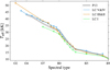 |
Fig. 1. Derived relations of spectral types and effective temperatures (crosses) for different luminosity classes (LCs). The solid gray line shows the relation for Galactic dwarf stars (P13; Pecaut & Mamajek 2013). |
We were unable to convert the spectral type of 114 sources in the B10 data set into a temperature (e.g., ‘Be? + XRB’). We applied the spectral type – Teff relations to infer effective temperatures for the remaining 5155 sources. When the temperature was known, the bolometric correction (BC) in the G band was taken from the MIST (Dotter 2016; Choi et al. 2016) website2. Because the surface gravity of most of the sources in the B10 data set is unknown, we used the BCs for log g = 3. At higher and lower log g, these BCs match temperature values that are typically well within 1 kK. In the B10 data set, 116 sources have the label ‘binary’. We used the spectral type that is mentioned first for them and further treated them as single stars. We highlight them in Fig. B.10.
For stars in the VSS sample, we compared the Gaia colors that are predicted for their effective temperatures to their observed Gaia colors. The predicted colors are calculated as BC(GBP)−BC(GRP) as given by MIST. We find that the predicted and observed colors match best for a reddening of E(GBP − GRP) = 0.14. This value corresponds to an extinction of AG = 0.28 in the G band and AV = 0.35 in the V band (Table 3 from Wang & Chen 2019, see also Gordon et al. 2003). We use these extinction values throughout the paper.
Furthermore, we adopted a distance modulus (DM) of the SMC of 18.91 (Hilditch et al. 2005). Then we calculated the absolute bolometric magnitude of a source using
 (1)
(1)
which is translated into luminosity using log(L/L⊙) = − 0.4(Mbol − Mbol, ⊙). Here, we adopt a solar value of Mbol, ⊙ = 4.74.
To test this method, we show the luminosities of the sources brighter than log(L/L⊙) = 4.5 in Fig. 2 for the sources that are included in the VSS sample and in the B10 data set. On the y-axis we show the difference between the luminosity reported in the VSS sample and the luminosity we obtained with our method based on the B10 data set. The black line, showing a linear fit, indicates that there is no systematic offset between the luminosities derived by our B10 method and the VSS literature values. The values of log(LVSS/L⊙)−log(LB10/L⊙) have a standard deviation of σ = 0.13 dex.
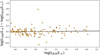 |
Fig. 2. Difference between the logarithm of the luminosities reported in the various spectroscopic studies (VSS) sample and those derived by our method using spectral types of B10 as a function of log(LB10/L⊙). Each dot represents an individual source. The dotted line shows where LB10 = LVSS; the solid line is a linear fit to the scatter points. |
2.2. Investigating the completeness with Gaia photometry
Although the B10 catalog contains more stars than the VSS sample, it still does not contain all of the brightest stars in the SMC. We can expect the Gaia data to be much more complete. This is supported by the fact that we found a Gaia counterpart for 99.6% of the B10 sources; see also a discussion of this in Appendix B.1. Unfortunately, however, Gaia colors are less accurate in determining effective temperatures (and therefore luminosities) than spectral types, and the results strongly depend on extinction. This is especially true for the hotter stars.
Using Gaia colors and magnitudes, we therefore cannot individually derive reliable luminosities for our sources. However, the colors and magnitudes can be used to estimate the completeness of an ensemble of stars, in this case, the B10 catalog. With ‘completeness’ we mean the completeness fraction of hot, bright stars that can be identified as such by the relevant observational approaches, that is, spectroscopy, and/or photometry in the optical.
We used Gaia photometry, and again MIST BCs, to calculate the photometric temperature and luminosity of the B10 and Gaia sources3: Teff, phot and Lphot. We then plotted them in an HRD that we refer to as the ‘photometric HRD’ (Fig. 3). Next, we used this HRD to estimate the completeness of the B10 catalog as a function of luminosity. For this estimate we also used an HRD for which we used B10 spectral types instead of Gaia colors (Fig. 5), as we explain below. We only considered temperatures above Teff = 103.8 K because for cooler temperatures we rely on the results of Davies et al. (2018) on cool, bright SMC stars. The way we operate is described below.
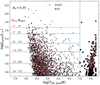 |
Fig. 3. Hertzsprung-Russell diagram of bright SMC sources constructed with Gaia photometry. Black markers indicate sources from the Gaia sample. The smaller red markers are sources in the B10 sample. Therefore, red points with black edges (all but one of the red points, see Appendix A) are sources that are listed in both samples. We count the number of sources that are hotter than 103.8 K for both samples in different luminosity intervals. The numbers are displayed on the left side of the plot. The luminosity intervals are indicated by dashed blue lines. For completeness, we also show the cool sources with crosses. |
1. We counted the number of sources in Fig. 5 in different luminosity intervals. The numbers are listed under NB10 in Table 1. For example, in Fig. 5 we count 15 stars above log(LB10/L⊙) = 5.75.
Number of stars with Teff ≳ 103.8 K counted in different luminosity intervals.
2. Then we examined the photometric HRD (Fig. 3), from high to low luminosity. In this example we considered the 15 brightest stars in B10, which represent the log(LB10/L⊙) > 5.75 bin.
3. We counted the number of Gaia sources until we found 15 sources that were also in the B10 catalog. We took this approach to have the same number of B10 sources in each luminosity bin. This counting in Fig. 3 took place in the intervals that are separated by dashed blue lines. They do not by definition coincide exactly with the luminosity intervals listed in the left column of Table 1. In this example at the bright end, we count NGaia, phot = 19. For the log(LB10/L⊙) > 5.75 bin, we thus estimate that it has a completeness fraction of 15/19 = 0.79.
4. We repeated this for each luminosity interval (i.e., also for 5.50 < log(LB10/L⊙) < 5.75 with the 16th to 42nd brightest star from the B10 catalog method, etc.) listed in Table 1 to calculate the completeness fraction of the B10 catalog: NB10/NGaia, phot.
Figure 3 and Table 1 show that the completeness level of the B10 catalog is 70%–80% for the brightest sources. The completeness drops below 40% around log(L/L⊙) = 4.5.
For this estimate to be reliable, the values of LB10 and Lphot need to be similar for most of the stars. We note that if Lphot had no predictive power, we would expect to measure the same completeness in all luminosity bins. We investigate this further in Fig. 4, where we compare Lphot of the sources to their VSS luminosity and the luminosity calculated using their B10 spectral type. This figure shows that while the scatter is large, the luminosities obtained with Gaia photometry on average give a good indication in which luminosity segment most sources belong.
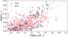 |
Fig. 4. Correlation between the luminosity of sources as calculated using their Gaia color and magnitude (Lphot) and the luminosity of the same source derived in various spectroscopic studies (VSS) or its luminosity based on the temperature derived from the spectral type listed in B10. |
In Appendix B.1 we provide another (simpler) test in which we count blue sources in the B10 and Gaia DR2 catalogs. The trends in this second test are very similar to those described in this section.
Both of our completeness tests imply a higher completeness than the completeness quoted for O stars in B10 itself (∼4%). However, their number is based on an estimate of 2800 O stars of M > 20 M⊙ from the conference proceedings of Massey (2010). This number is in turn based on UBV photometry from Massey (2002). In their Table 8b, all 70 blue stars that are known to have O types have a photometry-derived temperature in the O-star regime. Because of the uncertainties in determining the temperatures of hot stars with photometry (e.g., Massey 2003), this means that flagging many B-type stars as O-type stars seems unavoidable with this method. This has also been argued by Smith (2019), and we refer to Appendix B.1 for a quantitative discussion that supports this view. It therefore seems likely that the O-star completeness fraction quoted in B10 is severely underestimated.
In the Simbad catalog4, we inspected the four most luminous sources in Fig. 3 that are not in the B10 catalog. From high to low luminosity in Fig. 3, these are (i) Sk 177 (Sanduleak 1969) with the unusable spectral type information of ‘OB’; (ii) the O5.5 V star of log(L/L⊙) ≈ 5.3 in Lamb et al. (2013); (iii) Sk 183, which is an O3 V star with log(L/L⊙) = 5.66 (Evans et al. 2012); and (iv) a source without information on spectral type.
We return to the luminosity-dependent completeness fraction presented in Table 1 in Sect. 4.4. There we discuss the luminosity distribution of stars in the B10 sample and compare it with theoretical predictions.
3. General population properties
Figure 5 shows the distribution of the B10 sources in the HRD. It contains 780 stars with Teff > 103.8 K that are more luminous than 104.5 L⊙. Below Teff = 103.8 K, we rely on the red supergiant (RSG) sample of Davies et al. (2018), which we overplot on the HRD. To avoid duplicates, the B10 sources in this low-temperature regime are not considered in the rest of the paper. In Sect. 4 we discuss the main features of the stellar population shown in Fig. 5. We first describe a number of checks that we performed.
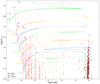 |
Fig. 5. Hertzsprung-Russell diagram of luminous stars in the SMC. Red dots represent sources from the B10 data set. Open dark red squares are red supergiants from Davies et al. (2018), where the Teff is obtained using relations from Tabernero et al. (2018). We show the Wolf-Rayet stars (Hainich et al. 2015; Shenar et al. 2016, 2017) labeled with a ‘W’ and their identifying number. Whe they have an O-star companion that is brighter in the V-band, we show this instead (indicated by ‘(O)’). We also show evolutionary tracks of Schootemeijer et al. (2019) with a semiconvection parameter of αsc = 10, and an overshooting parameter of αov = 0.33. Solid lines indicate hydrogen- and helium-core burning phases; dashed lines indicate the in between phase. The dash-dotted gray line shows the location of these models halfway through their main-sequence (MS) lifetime, tMS. |
In Fig. B.5 we compare the HRD positions of stars in Fig. 5 to their HRD positions according to the VSS sample (if they are in the VSS sample). We note that they match reasonably well, as is the case for the derived luminosities (Fig. 2).
When we calculate the extinction for each star individually (Fig. B.6, and see Sect. 3.1) instead of assuming a constant AV = 0.35, the shape of the population does not significantly change compared to the population shown in Fig. 5. A difference is that with individually calculated extinction, we find more stars above the 40 M⊙ track. However, compared to the VSS sample, the luminosities of the brightest stars are then systematically overestimated (Fig. B.4). On the other hand, a constant AV = 0.35 does not result in a systematic offset for the brightest stars (Fig. 2). Moreover, with variable extinction, the standard deviation in log(LVSS/L⊙)−log(LB10/L⊙) is the same (0.13 dex) as with the constant AV = 0.35. For these reasons, we use AV = 0.35 in our main HRD (Fig. 5).
The shape of the population also remains almost intact when different spectral type – temperature relations are used, as we show in Fig. B.7. The same is true when we take a different input catalog (Fig. B.8, where we use Simbad instead of B10). This demonstrates that the results we present later on are robust against the choice of assumptions described in Sect. 2. For the sources shown in Fig. 5, we also calculated the distribution of the visual extinction AV (Sect. 3.1), the ionizing photon production rate (Sect. 3.2), and estimate the implied star formation rate (SFR; Sect. 3.3).
3.1. Extinction
We calculated the extinction sources in the B10 data set with a luminosity of log(L/L⊙) > 4.5. In order to do so, we employed the effective temperature and resulting expected intrinsic color (GBP − GRP)int, which we obtained as described in Sect. 2.1. We then obtained the reddening as E(GBP − GRP) = (GBP − GRP)obs − (GBP − GRP)int, where (GBP − GRP)obs is the observed Gaia color. Then we calculated the extinction in the V band as AV = 2.42 ⋅ A(GBP − GRP). This relation is obtained from values in Table 3 of Wang & Chen (2019). More details are given in Appendix B.2.
Figure 6 displays the resulting AV distribution. It shows that most stars have an extinction of AV = 0.3–0.5. The distribution has a second peak slightly above AV = 1 that is mainly caused by Be stars; these tend to be redder than what would be expected for their spectral type. This results in a higher inferred value for AV. The brightest stars also tend to have a slightly higher extinction, although only modestly so. For AV/E(B − V) = 2.74 in the SMC (Gordon et al. 2003), the peak in the AV distribution that we find agrees reasonably well with the canonical SMC reddening value of E(B − V) ≈ 0.1 (e.g., Massey et al. 1995; Górski et al. 2020).
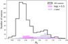 |
Fig. 6. Distribution of the visual extinction AV in the B10 sample when measured for each source individually. We also show the AV distribution of the subset for which we derive a luminosity higher than log(L/L⊙) = 5.5, and the subset of stars with an ‘e’ label in the B10 data set. |
3.2. Ionizing radiation and its escape fraction
Potsdam Wolf-Rayet (POWR) stellar atmosphere models (Hamann et al. 2006; Todt et al. 2015; Hainich et al. 2019) provide predictions for the ionizing photon production rate (Q) of bright SMC stars. We used them to calculate the H I, He I, and He II ionizing photon production rate of the 780 stars shown in our HRD (for details, see Appendix C). Figure 7 shows the resulting cumulative distributions. For comparison, we also calculated the ionizing photon production rate of a synthetic population of 780 stars from the single-star models of Schootemeijer et al. (2019), adopting random ages, which is displayed in Fig. 10 (for details, see Sect. 4.3). The synthetic population of bright SMC stars emits more ionizing radiation than the observed population in Fig. 5, while both contain the same number of stars. The difference is largest for He II ionizing radiation, which depends on the presence of a few hot stars. The reason for this large difference is that we find few young stars in the observed population. We discuss this dearth of young stars in Sect. 4.3.
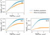 |
Fig. 7. Diagram of the cumulative distribution of the ionizing photon production rate Q. The stars in this cumulative distribution are sorted from a high to low Q. |
We find that the observed population shown in Fig. 7 emits about log Q = 2 ⋅ 1051 photons per second that are energetic enough for H I ionization. In addition to this, the Wolf-Rayet (WR) stars contribute half as many, 1051 H I ionizing photons per second, which means a total of 3 ⋅ 1051 H I ionizing photons per second. For He I ionizing photons, on the other hand, WR stars emit about a factor four more than the observed population of Fig. 7. He II ionizing radiation is dominated by WR stars by two to three orders of magnitude.
For H I ionizing photons, we can compare the numbers discussed above with observations. The SMC has an integrated Hα luminosity of 4.8 ⋅ 1039 erg s−1, which, assuming Q(H α) = 7.1 ⋅ 1011LH α ⋅ erg−1, translates into a production rate of 3.5 ⋅ 1051 H I ionizing photons per second in the SMC (Kennicutt et al. 1995). This is under the rough assumption that all the H I ionizing photons are absorbed by neutral hydrogen. Given the uncertainties, this number agrees well with the number of 3 ⋅ 1051 that we inferred for the observed massive star population, as discussed above.
We also estimated an upper limit to the escape fraction of H I ionizing radiation, fesc. We defined fesc as the fraction of photons that reaches our galaxy unhindered after being emitted by a star in the SMC. H I ionizing photons can be absorbed by dust or neutral hydrogen. We emphasize that for this upper-limit estimation of fesc, we only took the dust component into account. Gordon et al. (2003) provided extinction ratios toward λ = 91 nm (i.e., H I ionization threshold). The lowest wavelength they included is 116 nm, where A116 nm/AV = 7.0. In the following estimate, we adopt this extinction value also for λ < 116 nm. Alternatively, we could extrapolate the Gordon et al. (2003) extinction law to 91 nm to obtain A91 nm/AV = 9.7. When we subtract a Milky Way foreground extinction of AV = 0.18 (Yanchulova Merica-Jones et al. 2017) from the values discussed in Sect. 3.1, the typical V-band extinction of stars in the SMC itself is AV ≈ 0.2. In the H I ionizing photon regime, the expected extinction would therefore be A91 nm = 7.0 ⋅ 0.2 ≈ 1.4. This translates into fesc = 10−1.4/2.5 = 0.28. This number would decrease when the extinction continued to decrease with λ below 116 nm. For the extrapolated Aλ ≲ 91 nm = 9.7 ⋅ 0.2 = 1.94, fesc would be 0.16. If a significant fraction of stars is deeply embedded (Sect. 6.2), this number would also decrease. Moreover, the H I absorption term would still need to be added. Earlier in this section, we showed that the H α flux of the SMC matches the H I ionizing photon production rate well. This implies that most of the H I ionizing photons are already absorbed by neutral hydrogen. Combining the above, it seems most probable that fesc in the SMC is far lower than our upper limit of 0.28.
3.3. Star formation rate
Using a Kroupa (2001) IMF to extrapolate toward lower mass stars, we calculated the SFR of the SMC. To do this, we counted the number of stars above the 18 M⊙ track (Appendix C), assuming constant star formation (CSF). We find a current SFR of ∼0.018 M⊙ yr−1. This is below the typical literature value of ∼0.05 M⊙ yr−1 (Kennicutt et al. 1995; Harris & Zaritsky 2004; Wilke et al. 2004; Bolatto et al. 2011; Hagen et al. 2017; Rubele et al. 2015, 2018). We note that previous studies (except Kennicutt et al.), which used deep photometry, were not tailored to resolve the SFR on timescales as small as the last 10 Myr.
In Sect. 4.3 we consider scenarios in which the SFR is not constant. In the best-fitting scenario (where the present-day SFR is relatively low), the SFR 7 − 10 Myr ago was about three times higher than for the CSF scenario. This would result in an SFR of ∼0.05 M⊙ yr−1 in this period, which matches the literature values mentioned above. However, then the present-day SFR would be even farther below the literature value.
Alternatively, we could assume that the IMF in the SMC is steeper. Because our method is based on counting massive stars, a steeper IMF would result in a higher inferred SFR. Then, for CSF, to obtain an SFR of 0.05 M⊙ yr−1 instead of 0.018 M⊙ yr−1, an IMF exponent of Γ = −1.6 is needed (Appendix C).
4. Features in the Hertzsprung-Russell diagram
4.1. Blue supergiants
Interestingly, about 200 stars in Fig. 5 reside in the region between the main sequence (MS) and the RSG branch. The exact number of stars in this region depends on the location of the terminal-age main sequence (TAMS). Theoretically, this is affected by the choice for the overshooting parameter (Maeder 1976; Vink et al. 2010), and by rotation (von Zeipel 1924).
A significant fraction of the stars roughly 0.05 − 0.1 dex (2 − 5 kK for Teff, TAMS = 25 kK) to the right of the TAMS shown in Fig. 5 are Be stars (as is also the case in Fig. 13 of Ramachandran et al. 2019). We highlight stars with emission features (indicated by their B10 spectral type and/or infrared excess) in Fig. B.10. Emission features make it likely that these are late-MS stars that evolved toward critical velocity in isolation (Ekström et al. 2008; Hastings et al. 2020) or were aided by a binary companion (e.g., Gies et al. 1998; Schootemeijer et al. 2018; Wang et al. 2020) rather than He-burning blue supergiants. The offset of 0.05 − 0.1 dex is in line with a shift in Teff of 0.05 dex at critical rotation (Paxton et al. 2019), uncertainties in overshooting (see Schootemeijer et al. 2019), and modest errors. For stars in Fig. 5 at Teff ≲ 104.3 K (∼20 kK) below log(L/L⊙) ≈ 5.5, it appears more likely that they are helium burning because the emission features almost completely disappear (Fig. B.10) and this temperature range can be covered by post-MS tracks (Schootemeijer et al. 2019) as well as by the post-binary-interaction models of Justham et al. (2014). We argue that it is unlikely that many H-burning stars can be found in Fig. 5 below 20 kK and log(L/L⊙) < 5.5. The reason is that very high overshooting values of αov = 0.55 are necessary for the TAMS to extend that far (Schootemeijer et al. 2019). Even then, we do not expect many MS stars at 20 kK because these models spend 95% of their MS lifetime at Teff < 25 kK.
Single-star evolution models of massive stars without efficient semiconvective mixing (e.g., Brott et al. 2011) cross the inter-MS-RSG region rapidly and spend only about 0.1% of their lifetime there. This means that if the SMC population exclusively consisted of single stars without efficient semiconvection, only about one star would reside between the MS and the RSG branch. In contrast, our HRD shows that there are least a hundred, even when the TAMS lasts 0.1 dex longer than the TAMS of the models shown in our HRD. It therefore appears to be unavoidable to invoke either internal mixing (Langer 1991; Stothers & Chin 1992; Schootemeijer et al. 2019) or binary interaction (Braun & Langer 1995; Justham et al. 2014) to explain their presence.
To obtain further clues, we suggest to investigate the binary properties of the blue stars in Fig. 5 with Teff ≲ 20 kK and log(L/L⊙)≳5. The detection of a close MS companion would be a strong indication that such a star is following a single-star track that moves to the RSG branch on a nuclear timescale, rather than being on a blue loop or being a merger product. There is evidence, however, that the binary fraction of massive stars decreases toward later spectral types (Dunstall et al. 2015; McEvoy et al. 2015, Simón-Díaz et al., in prep.). This would therefore provide a crucial test for existing evolutionary models of low-metallicity massive stars (e.g., Brott et al. 2011; Georgy et al. 2013; Limongi & Chieffi 2018; Schootemeijer et al. 2019).
4.2. Numbers of helium-burning stars and their progenitors
We counted the helium-burning stars and compared the corresponding expected number of hydrogen-burning stars (based on stellar models) with the observed number of hydrogen-burning stars. The lowest initial mass that we considered is 18 M⊙. This is the minimum mass where the zero-age main-sequence (ZAMS) models are bright enough to be in the luminosity range of our HRD. This is shown in Fig. 8, where we illustrate the method used in this exercise. The 18 M⊙ evolutionary track has a time-averaged luminosity of log(L/L⊙) = 5.1 during helium burning. The most luminous RSG in the sample of Davies et al. (2018) has log(L/L⊙) = 5.55, which corresponds to the time-averaged helium-burning luminosity of a evolutionary 29 M⊙ track. The red box in Fig. 8 (with 5.1 < log(L/L⊙) < 5.55) represents the temperature and luminosity range of 18 to 29 M⊙ RSGs, and contains observed 24 RSGs. In Sect. 4.1 we argued that stars in our HRD below 104.3 K ≈ 20 kK are most likely helium burning. In the luminosity range described above, we count 25 blue stars below 20 kK. This makes a total of 24 + 25 = 49 helium-burning stars with initial masses between 18 and 29 M⊙ (and a ratio of blue to red supergiants of about one). These models have a fractional helium-burning lifetime of about 7% (e.g., Schootemeijer et al. 2019). We therefore expect ∼650 progenitor stars. A total of 229 MS stars shown in Fig. 5 lie between the 18 and 29 M⊙ evolutionary tracks at Teff > 20 kK. Corrected for a completeness of about half (Table 1), this adds up to ∼450 progenitor stars. This poses a modest discrepancy with the expected 650. If all stars in this mass range down to 16 kK were MS stars, then only ∼500 progenitor stars would be required. However, we do not expect this to be the case (Sect. 4.1). On the contrary, with the already conservative value of 20 kK, we most likely exclude some number of helium-burning stars. In this case, more helium-burning star progenitors are required, which increases the discrepancy. The presence of about two out of three (450 out of 650) helium-burning star progenitors in the 18 − 29 M⊙ initial mass range should therefore be considered an upper limit.
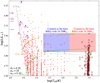 |
Fig. 8. Hertzsprung-Russell diagram showing the same SMC objects as Fig. 5, indicating which stars are considered as He-burning stars with initial masses between 18 and 29 M⊙. The tracks are from the extended grid of Schootemeijer et al. (2019). |
We performed a similar exercise for WR stars. These stars are thought to be complete in the SMC (Neugent et al. 2018). In the 12 WR star systems, 7 are apparently single (Hainich et al. 2015) and 5 are binary systems (Shenar et al. 2016). Nine of the 12 WR stars are so hot that only core helium-burning models can explain them (Schootemeijer & Langer 2018). They have inferred initial masses in excess of ∼40 M⊙ (Hainich et al. 2015; Shenar et al. 2016; Schootemeijer & Langer 2018). The fractional core helium-burning lifetime of such stars is about 7% (Schootemeijer et al. 2019). This suggests the presence of at least 100 hydrogen-burning progenitors with masses in excess of ∼40 M⊙. We count 22 red circles above the 40 M⊙ track in Fig. 5. For an 80% completeness (Table 1), this results in an estimated ∼27 progenitors, only a quarter of the expected number. Even given some uncertainties in the minimum initial mass of SMC WR stars, this discrepancy is stronger than for the blue supergiants (BSGs) and RSGs discussed above.
4.3. Age and relative age distribution
The gray dot-dashed line in Fig. 5 denotes the location of stars that are halfway through their MS lifetime. Only a few stars lie to the left of this line. In a scenario in which star formation is constant, we would expect roughly half of the observed sources to reside to the left of this line. To further investigate this, we obtained the age and fractional lifetime of the stars in our sample. We did this by comparing them with evolutionary models of Schootemeijer et al. (2019) shown in Fig. 5, but using a denser grid with a spacing of 0.02 dex in mass. The inferred age and fractional age (i.e., age divided by stellar lifetime) are those of the nearest stellar model.
In Fig. 9 the distributions of these inferred ages (bottom right) and fractional ages (bottom left) are shown with a gray line. In this plot, we only show sources with Teff > 103.8 K and evolutionary masses above 18 M⊙. The distribution is therefore not affected by a luminosity cutoff. Instead of ∼50% of the stars being in the first half of their MS lifetime, this number is only 7% for the B10 sample. For the stars in the VSS sample, this fraction is about 20%, which is less extreme, but still much lower than expected. One explanation for this slight difference between the B10 and VSS samples is that our method could underestimate Teff, which would increase the inferred age. However, no such systematic trend is visible in Fig. B.5. Another possible explanation is that there could be a stronger observational bias against hot stars (compared to cool stars) in the B10 catalog, but as we discuss in Sect. 6.1, we do not expect this effect to be strong. More likely, the explanation for the relatively larger fraction of young stars in the VSS sample could be that this sample is biased towards hot stars simply because of a greater interest in them, and young massive stars tend to be hot. This is supported by Fig. 3, which shows that the B10 catalog is rather complete for hot and bright stars.
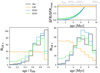 |
Fig. 9. Fractional age (bottom left) and absolute age (bottom right) distribution of the number of stars that are above the 18 M⊙ track (referred to as N18+) in Fig. 5. The colored distributions are theoretical predictions for CSF, and two other star formation histories (SFH2 and SFH3) where young stars have a lower probability (top right panel). The gray line indicates the distribution that we derived using observations. |
We investigate in Fig. 9 whether a decreasing SFR can explain this heavily lopsided distribution of relative ages. From the model population, we drew 106 stars with random ages between 0 and 10 Myr, and random masses between 18 and 100 M⊙. Then, we weighted these model stars by the Salpeter initial mass function (IMF; Salpeter 1955) and normalized their number to the number of observed stars. Stellar models with Teff < 103.8 K and models that live shorter than the drawn age were discarded. The bottom left panel of Fig. 9 shows that for CSF, the synthetic relative age distribution is flat, as is expected, but at odds with observations. In the last bin, the number drops because RSG models are not included.
Next, we considered a star-formation history (SFH) scenario, SFH2, that mimics the observed age distribution. There, the SFR is set to zero at an age of 0 Myr and then increases with age to the third power up to 7 Myr; then it stays constant (i.e., we reduce the probability to draw younger stars; Fig. 9, top panel). The resulting synthetic relative age distribution with SFH2 also fits the observed distribution well, at least up to age/tlife = 0.9. Finally, we considered SFH3, which is the same as SHF2 except that the SFR starts at 10% of the final SFR. We display SFH3 to illustrate how dramatic the drop in SFR needs to be to match the observations. Even this rapid 90% drop in SFR still strongly overpredicts the number of relatively young stars, especially at age/tlife < 0.3 and ages below ∼3 Myr. We conclude that the observed relative age distribution can be reconciled only if the SFR has dropped to essentially zero in the last few million years. The implication of this would be that the SMC contains about 20 stars over 18 M⊙ in the first half of their lifetime, and more than 300 in the second half of their lifetime. In other words, assuming CSF, about 300 stars above 18 M⊙ in the first half of their lifetime are missing.
In the bottom right panel of Fig. 9 we show the corresponding absolute age distributions. Models that are initially more massive than ∼25 M⊙ live shorter than 10 Myr. As a result, in the CSF scenario the shape of the age distribution is shifted toward younger ages, in stark contrast to the distribution that is observed. Again, the observed distribution matches well for SFH2, while in the SFH3 scenario the number of young stars is higher than what is inferred from observations.
Most of the time, massive stars become cooler as they evolve. Therefore our inferred lack of young stars goes hand in hand with a lack of stars with very early spectral types. This is quantified in Table 2. The numbers that we derive are based on the amount of time spent by our evolutionary models in the different temperature ranges, weighted by the Salpeter IMF. We show a synthetic population in Fig. 10. There we have drawn 780 stellar models with a probability that is based on how long-lived they are and on the IMF. The upper mass limit of the models is 100 M⊙. The discrepancy is quite extreme: for example, we expect 110 stars of type O5 or earlier, but only 14 are in our sample.
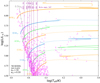 |
Fig. 10. Same as Fig. 5, except that it contains randomly drawn synthetic stars (purple crosses) and that the x-axis range does not extend to the temperature regime of red stars. The dashed lines separate the temperature ranges covered by different spectral types of luminosity class V, according to our spectral type-temperature relation (Sect. 2.1). |
4.4. Luminosity distribution
The left panel in Fig. 11 shows the luminosity distribution of the stars shown in our HRD (referred to as ‘observational’; Fig. 5). We consider the 780 sources from the B10 data set with Teff < 103.8 K and log(L/L⊙) > 4.5. To show that the WR sources affect the luminosity distribution to a limited extent, we also show it including the visually brightest components of the WR systems. To obtain the error bars, we randomly scattered the luminosities of all individual sources by a value drawn from a Gaussian distribution with σ = 0.13 dex (i.e., the error on the luminosity that we derived in Sect. 2.1). We did this 250 times. The shown error bars represent the standard deviation of the number of stars in each bin after scattering.
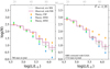 |
Fig. 11. Diagrams showing the high end of the distribution of luminosities that we derived for sources in the Bonanos et al. (2010) data set. Left is the uncorrected distribution. Right is the distribution corrected for the completeness of the B10 data set using Gaia data. For comparison, we show the theoretical values (diamonds) for different star formation history scenarios. We also show the number distributions when the brightest source in the WR star system is taken out. |
We compared this with theoretical luminosity distributions (models of Schootemeijer et al. 2019, as in Sect. 4.3) for the same total number of stars as quoted above (780). When we computed this distribution, we assumed a Salpeter IMF while also taking the model lifetimes (where Teff > 103.8 K) into account. To cover the log(L/L⊙) = 6–6.25 bin with ZAMS models as well, we extended the initial mass range to 126 M⊙. The observed population has fewer sources at the luminous end than the theoretical CSF populations with and without WR systems. At log(L/L⊙) > 5.5, the difference is about 0.3 dex, which is a factor two. When we consider different SFHs, SFH2 (for which the SFR is essentially zero in the last few million years) on the other hand predicts fewer sources with log(L/L⊙) > 5.5 than are observed. SFR3 provides the best fit to the distribution that is not corrected for completeness, with only a slightly smaller difference to the observed distribution than for the CSF scenario.
We show the observed luminosity distributions corrected for completeness in the right panel of Fig. 11. We deem these to be the most realistic. To obtain the values, the number of sources in the luminosity bins in the left panel was divided by their completeness fraction listed the right column of Table 1. The corrected distribution is steeper because the completeness correction is larger at lower luminosities. The theoretical distributions in this panel are again scaled to the total number of observed stars, which is 1714 after completeness correction. Then, the theoretical SFH3 distribution matches the observed distribution best. The theoretical CSF distribution contains many more bright stars than the observed distributions. When observed WR stars are included, the difference is ∼0.6 dex, or a factor four.
This means that not only young stars (Sect. 4.3), but also bright stars appear to be rarer than expected in the SMC if its star formation were constant. We discuss possible reasons for this in Sect. 6.1.
We also varied the IMF to see where we achieve the best fit of the theoretical luminosity distribution (assuming CSF). The uncorrected luminosity distribution is fit best for Γ ≈ −1.9. For the luminosity distribution that is corrected for completeness, Γ ≈ −2.3 fits best. When we calculate the extinction individually per star (as we do in the HRD shown in Fig. B.6), these numbers become ∼−1.7 and 2.1, respectively). This means that in principle, we can resolve the lack of bright stars by assuming a steeper IMF. However, this does not resolve the problem with the dearth of young stars.
5. Number comparisons
In this section we discuss the number of massive SMC stars obtained by previous studies. We note that we count only one star in a binary (or higher order multiple) because of the lack of completeness of the information on binarity, and the biases therein. We compare the derived numbers with our results, which we also summarize here.
We first discuss the studies of the SMC massive star population that have been performed before (Humphreys & McElroy 1984; Blaha & Humphreys 1989; Massey et al. 1995). We note that these studies lacked stars above V = 15, which is the ZAMS magnitude of a 40 M⊙ star in the SMC. Above the 40 M⊙ track, to the right of the ZAMS, we find similar numbers of stars as these studies. When stars in WR systems are excluded and completeness is not corrected for, Fig. 5 contains 22 of such massive stars (Sect. 4.2). The number of SMC stars above 40 M⊙ is 21 according to Blaha & Humphreys (1989) and 32 according to Massey et al. (1995).
Based on the Salpeter IMF, model lifetimes, random ages, and an upper mass limit of 100 M⊙, we expect 75.6 model stars out of the 780 shown in Fig. 10 to lie above the 40 M⊙ track. We randomly drew 72. Compared to the 22 stars in the B10 data set above the 40 M⊙ track, this amounts to a difference of a factor 75.6/22 = 3.4. This is in line with the 0.5 dex difference between the uncorrected theoretical CSF luminosity distribution and the observed distribution without WR stars above log(L/L⊙) = 5.5 in the left panel of Fig. 11. The difference in the 5.5 < log(L/L⊙) < 5.75 bin is smaller, but we note that many of the stars in this bin are located below the 40 M⊙ track. This discrepancy can be expected to be slightly larger after correcting for completeness, even after adding the WR stars (cf. the left and right panels in Fig. 11).
We can also estimate how many of these very massive stars with M > 40 M⊙ (N40+) are expected when a constant (typical) SFR of ∼0.05 M⊙ yr−1 is assumed. Repeating the exercise described in Appendix C for M > 40 M⊙ yields a fraction of f40+ = 0.075 of the stellar mass budget that is tied in stars with M > 40 M⊙. Moreover, the IMF dictates that the average mass of stars of higher mass than 40 M⊙ has a value of  M⊙ (again assuming an upper mass limit of 150 M⊙). Such massive models have an average lifetime of
  Myr (e.g., Schootemeijer et al. 2019). We have approximate values for the rate at which gas is converted into M > 40 M⊙ stars, and for their typical mass and lifetime. We combined these for our estimate and filled in the values:
  . This number is about a factor 6 − 7 higher than the total number of ∼40 stars with initial masses above 40 M⊙ that we find in the SMC.
In Sect. 3.2 we estimated that the H I ionizing photon production rate of the observed massive star population is about 3 ⋅ 1051 photons per second. This agrees well with the rate of 3.5 ⋅ 1051 photons per second that is inferred from the H α luminosity of the SMC. In Sect. 3.3 we found that the literature SFR value for the SMC (∼0.05 M⊙ yr−1) does not match the value we derived assuming CSF (∼0.018 M⊙ yr−1). However, the value did match for 7 − 10 Myr ago if young stars are apparently rare.
In Sect. 4.2 we showed that WR star progenitors are underabundant, even after correcting for completeness. We estimated that only 27 out of ∼100 of these objects are detectable in the SMC. At lower luminosity, we found the same discrepancy, although the difference was smaller. For helium-burning BSGs and RSGs with 5.1 < log(L/L⊙) < 5.55, we inferred that at most two out of three progenitors are present.
In conclusion, the numbers that we find appear to agree with literature studies on the massive star population in the SMC. However, the number of observed of stars with M > 40 M⊙ is much lower than what would naively be estimated from both the SFR of the SMC (by a factor 6 − 7) and the total number of stars with log(L/L⊙) > 4.5 (by a factor 3 − 4). The number of helium-burning star progenitors is also significantly lower than we would expect a priori. These underabundances are in line with a bias against young stars, or with them being absent due to a plummeting SFR (Sect. 4.3).
6. Discussion
6.1. Possible explanations for a dearth of young and bright stars
Above, we have identified two types of stars that are more rare than would naively be expected: those that are in the first half of their MS lifetime (Sect. 4.3), and those that are brighter than log(L/L⊙) = 5.5 (M ≳ 40 M⊙; Sect. 4.4). Below, we discuss the likelihood of several potential explanations.
6.1.1. Steeper initial mass function
In principle, a steeper IMF could help to explain the lack of bright stars. An exponent of Γ = −2.3 would be required to explain the completeness-corrected luminosity distribution that we show in the right panel of Fig. 11, under the assumption of CSF. This is much steeper than the Salpeter exponent of Γ = −1.35. A steeper universal IMF would have dramatic implications for the early universe because it is commonly thought that toward lower metallicity, massive stars become more common (Larson & Starrfield 1971; Schneider et al. 2018a). However, this is currently an unsatisfying explanation because it cannot resolve the apparent lack of young stars. An explanation that would have to be ruled out is a bias against young stars (Sect. 6.1.6): because very massive stars (which live only for a short time) tend to be young, such a bias would make the IMF appear steeper than it really is. Moreover, the SFR in the SMC could be low enough for stochasticity to play a role (see da Silva et al. 2012).
6.1.2. Model uncertainties
In principle, the stellar models of Schootemeijer et al. (2019) that we used could overpredict stellar temperatures and therefore the inferred stellar ages. First, an aspect that we did not consider when we derived the age distribution is rotation. Rotation can reduce the effective temperatures of stars. We performed a small experiment where we shifted the gray line in shown in Fig. 5 (where stars are halfway through their MS lifetime). Our finding is that in order to have half of the sources that are shown in Fig. 9 (i.e., those above the 18 M⊙ track) on the hot side of this line, the line needs to be shifted to lower temperatures by 0.09 dex. This is significantly larger than the shift of 0.05 dex for stars at critical rotation (Paxton et al. 2019). Furthermore, most stars in the SMC are not close to critical rotation, but typically at most at half critical (e.g., Mokiem et al. 2006; Ramachandran et al. 2019). In this case, the shift in effective temperatures would be about ∼0.01–0.02 dex or less (see Sect. 4.1), which is far below the required 0.09 dex. In the most extreme cases, rapid rotation could induce mixing strong enough for chemically homogeneous evolution to take place (e.g., Maeder 1987; Langer 1992; Brott et al. 2011; Aguilera-Dena et al. 2018). Then, stars maintain high effective temperatures and stay close to the ZAMS during hydrogen burning. This means that chemically homogeneous evolution would not help either to solve the problem of too many stars being observed with relatively low temperatures.
As a second possibility, envelope inflation could reduce stellar effective temperatures when stars approach the Eddington limit (Sanyal et al. 2015). However, this is expected to occur only at luminosities of roughly log(L/L⊙)≳5.75. Moreover, envelope inflation is less likely to occur in metal-deficient environments such as the SMC (Sanyal et al. 2017). Combined, this means that at least the vast majority of the stars in our analysis should be unaffected by envelope inflation. We conclude that rotation and envelope inflation are unlikely to affect our conclusions about the dearth of young stars. Moreover, these effects would not help to resolve the issue of missing bright stars.
Alternatively, Ramachandran et al. (2019) have suggested a transition at 32 M⊙ in the SMC, with stars below this initial mass experiencing ‘normal’ evolution, and heavier stars evolving chemically homogeneously. This is meant to explain why the distribution of their sample stars in the HRD avoids cool temperatures above the 32 M⊙ track (cf. their Fig. A.1) because homogeneously evolving stars have ZAMS temperatures or hotter and manifest themselves as WR stars. We note that in our Fig. B.5 the stars from Mokiem et al. (2006) with an ‘AzV’ label (that reside in the high-luminosity region between ZAMS and TAMS) are included, which is not the case in their figure. Moreover, the HRDs of Blaha & Humphreys (1989) and Massey et al. (1995) contain several tens of stars to the right of the ZAMS that are above a 32 M⊙ SMC track. The B10 sources that we analyzed also populate this region in the HRD (Fig. 5).
In addition to this, it has been shown that the eight out of nine WR stars that reside to the left of the ZAMS cannot be chemically homogeneous. The reason is that they show a significant amount of hydrogen at their surfaces, which means that if they were chemically homogeneous, they would burn hydrogen in their cores. However, they are far hotter than core hydrogen-burning models of Brott et al. (2011), for example. Schootemeijer & Langer (2018) have shown in a model-independent way that even hydrogen-poor chemically homogeneous SMC models in the WR star luminosity range burn hydrogen at Teff ≈ 50 − 60 kK (their Fig. 2), whereas these eight WR stars have an average effective temperature of 93 kK (Hainich et al. 2015; Shenar et al. 2016, 2018). Together with the absence of a void above the 32 M⊙ track in our (and others’) HRD, this appears to rule out the scenario with homogeneous evolution for all stars above 32 M⊙ at SMC metallicity.
6.1.3. Star formation history
At first sight, an SFH with a close-to-zero SFR in the last few million years is a tempting explanation. We have shown that it can explain both the lack of young and the lack of bright stars. However, it cannot do this simultaneously. SFH2 fits the age distribution and SFH3 fits the luminosity distribution, but neither fits both (Sect. 4).
We further discuss the decreasing SFR scenario in light of the SMC, LMC, and Milky Way environments. From an analysis of the positions and proper motions of the bright sources (Appendix D) in the SMC, we conclude that they cannot be traced back to one or a few production sites on the timescale of a few million years. If the SFH is the explanation for the inferred lack of young stars, the SFR accordingly needs to have been quenched throughout the entire SMC at the same time. It might be questionable whether this scenario is realistic. On the other hand, there is some evidence that the SFR in the SMC has changed on timescales of some tens of million years. From the high number of high-mass X-ray binaries in the SMC (about 150 – Haberl & Sturm 2016), it has been inferred that the SFR in the SMC peaked ∼40 Myr ago (Antoniou et al. 2010, 2019). Rubele et al. (2015) also inferred a recent peak in SFR, ∼20 Myr ago. However, no such peaks are present in their more recent work (Rubele et al. 2018, cf. their Fig. 11). Moreover, Harris & Zaritsky (2004) did not show such distinct peaks. However, in none of SFHs that are presented in these studies, the SFR drops by over 90% in just a few million years, as would be required for the SFH scenario to explain the dearth of young and bright stars.
A dearth of young massive stars has been seen in different environments. In the Milky Way, stars with evolutionary masses above ∼25 M⊙ close to the MS are nearly nonexistent in various samples (e.g., Castro et al. 2014; Holgado et al. 2018). Recently, it has been shown that this feature persists in a large and unbiased sample of 285 O-type stars (Holgado et al. 2020). As we discuss in Appendix B (see Fig B.9), the HRDs shown in these studies contain a void that spans nearly the entire temperature range of M ≳ 25 M⊙ stars in the first half of their MS lifetime. In the 30 Doradus starburst region in the LMC, the reported number density of massive stars that have just been born is three times lower than at ages of 2 − 4 Myr (Schneider et al. 2018b, their Fig. 3). In SMC-SGS1, a supergiant shell subregion in the wing of the SMC (see, e.g., Fulmer et al. 2020), it is inferred that recently born massive stars are about five times more rare than those with an age of ∼8 Myr (Ramachandran et al. 2019, their Fig. 17).
To summarize: it seems questionable that recently, star formation has essentially stopped on the timescale of a few million years throughout the entire SMC. It is even more unlikely that something similar happened in the two other local, but separated, star-forming environments: the LMC and the Milky Way. In addition, none of the considered star formation scenarios can explain the luminosity and age distributions simultaneously. The fact that at least several hundred massive young stellar objects (YSOs) as well as (ultra-)compact H II regions (see Sect. 6.1.6) are present in the SMC might further challenge this decreasing SFR scenario as the explanation for a dearth of young and bright stars.
6.1.4. Observational biases
Related to the ‘embedding’ scenario described below in Sect. 6.1.6, observational biases might be at play. Young massive H-burning stars are hot. As a result, they are relatively dim in the optical. This could cause a bias in the observed sample. However, the bulk of the considered sources comes from observational studies where a magnitude cut of about 17 was used. The 2dF survey (which comprises the vast majority of B10 sources) uses B ≲ 17.5 (Evans et al. 2004). Ramachandran et al. (2019), who adopted V < 17, showed that at the ZAMS their cut excludes M < 10 M⊙ stars (their Fig. 13). This shows that such magnitude cuts are not expected to exclude any stars that would be shown in Fig. 5. Still, a potential issue is that a mixture of selection effects influenced the final 2dF sample (e.g., crowding, color cut, possible saturation of the very brightest stars, and the spatial extent of both the input astrometry and spectroscopic observations). We note that sources precluded by the 2dF survey could still be in the B10 catalog. Furthermore, we show in Sect. 2.2 and Appendix. B.1 that the B10 sample is complete enough for biases not to affect our conclusions about the dearth of young and bright stars.
Another potential observational bias is crowding in dense clusters. At the distance of the Magellanic Clouds, crowding can hinder an accurate analysis of the residing stars (Evans et al. 2011). This could cause a dearth of bright young stars because they may prefer to live in unresolved clusters. If that is the case, these unresolved clusters should be detected as bright blue sources. The most luminous sources in the SMC according to Gaia photometry are shown in the top panel of Fig. 3. The ten brightest of these have well-determined spectral types (Sect. 2.2, last paragraph). There is no indication that they are unresolved bright clusters. Moreover, these sources are not bright enough to contain a large number of bright stars. From this, we conclude that the unresolved clusters required to explain the dearth of young stars are not in the Gaia catalog.
Next, we visually inspected UV images from Cornett et al. (1997), taken with the Ultraviolet Imaging Telescope (their Fig. 1), and Hagen et al. (2017), taken with the Swift telescope (their Figs. 2 and 3). The dominant UV sources in these papers are the clusters NGC 330 and NGC 346. They have recently been resolved and do not contain many, if any, early-O stars (O5 and earlier); see Bodensteiner et al. (2020) for NGC 330 and Dufton et al. (2019) for NGC 346. More specifically, the core of NGC 330 contains only two O-type stars, both of type O9e. NGC 346, which should be almost fully resolved according to Dufton et al. (2019), contains four sources of subtype O5 and earlier. All of these are in the B10 catalog. The lack of UV-bright sources other than NGC 330 and NGC 346 does not seem to leave room for unresolved clusters with a significant number of O2–O5 stars (Table 2 shows that naively, 110 of these stars are expected for CSF, but only 14 are known). To summarize: the Gaia catalog and UV images of the SMC show no indication of unresolved clusters hiding early-type O stars, and the few stars of type O5 and earlier that are in NGC 330 and NGC 346 are in the B10 catalog. Therefore we deem the unresolved cluster explanation to be highly unlikely, as long as the bright young stars are not embedded (Sects. 6.1.6 and 6.2).
Alternatively, the real temperatures of our sample stars could be higher than those that we derived based on the B10 spectral types. This would move them to higher luminosities as well. However, given that the temperatures and luminosities that we present agree reasonably well with the temperatures derived with atmospheric analyses (Fig. B.5), this would indicate a more severe problem than incorrect relations of spectral type and temperature.
6.1.5. Binary companions
About of half the sources in our HRD are expected to be binary systems (Sana et al. 2013) or even higher order multiples (e.g., SMC WR systems AB5 and AB6: Shenar et al. 2016, 2017). However, we treated all B10 sources as single stars (Sect. 2.1). The presence of unresolved binary companions could affect our analysis in two ways.
The first possible effect on our analysis caused by the presence of unresolved binary companions could be errors in the temperature and luminosity that we derive. We discuss this below. For a coeval equal-mass binary, we will derive a luminosity that is 0.3 dex higher than that of its individual components. Because luminosity scales strongly with mass, the error will be significantly smaller for unequal-mass binaries. A binary companion could also affect the spectral features of a source. To what extent this can change the apparent spectral types is not easy to gauge from first principles. We consider two extreme cases in a coeval binary. First, the equal-mass binaries are not affected because both components would have the same spectral type. Second, for systems where the spectral types of the components differ by more than a few subtypes, the effect should typically be minor because the spectrum is dominated by the massive component. In between these extremes, the single-star approximation could lead to modest errors in the derived temperature. In these cases, multi-epoch spectroscopy would be highly valuable to obtain more accurate measurements. To account for the dearth of young stars, we found that a systematic shift of 0.09 dex in temperature is required (Sect. 6.1.2). To illustrate: 0.09 dex corresponds to the temperature difference between an O7 V and a B0 V star. It is unlikely that unresolved binary companions could systematically shift the apparent spectral types of the population by that much.
The second possible effect of the presence of other stars within the sources that we analyzed is that it would add stars to the population that are now unaccounted for. This could affect the SFR and the number distributions that we derived. For the extreme case that all sources are equal-mass binaries, a naive guess is that we underpredict the SFR by a factor two. In reality, the impact of equal-mass companions would be smaller: the flux per star would be lower, such that in practice lower luminosities (and therefore masses) would be derived for the individual components. This effect of binarity could bring the SFR of 0.018 M⊙ yr−1 (assuming CSF; Sect. 3.3) closer to the literature value of 0.05 M⊙ yr−1.
For a scenario in which the binary fraction and mass ratio distribution do not depend on primary mass, we see no compelling reason for the shape of the age and luminosity distributions to change significantly. This would mainly affect the absolute numbers. A dependence of binary properties on primary mass may still exist, however (Moe & Di Stefano 2017). An explanation of the factor-of-a-few underabundance of WR star progenitors (Sect. 4.2) and of stars with log(L/L⊙) > 5.5 in the luminosity distribution (Sect. 4.4) would still require an extreme increase in multiplicity of stars towards the high-mass end. And again, if the most luminous stars are higher order multiples, the luminosity of the individual components would decrease, which works against this explanation. We conclude that the effects of binarity likely lead to typically modest individual errors, but that binarity alone cannot be expected to change the main conclusions of the paper on the dearth of young and bright stars.
6.1.6. Embedding in birth clouds
Another possible explanation for the lack of young and bright stars could be that young stars are still embedded in the clouds from which they are born. With increasing mass, the embedded phase is expected to last for an increasingly long fraction of the total lifetime (e.g., Fig. 1 of Yorke 1986). If this causes these objects to be hidden from our view, both young stars and bright stars would become more rare. We note that this would artificially steepen the IMF because brighter stars would then have a greater likelihood to be outside the sample.
For O-type stars in the Milky Way, it has been estimated that 10 − 20% of their MS lifetime is spent inside a molecular cloud (Wood & Churchwell 1989). Plausibly, metallicity can affect this number. Naively, we might expect young stars in low-metallicity environments to be less obscured because there is less dust. However, the situation might be more complex than that. For example, it might be speculated that at low metallicity, the relatively low amount of dust makes it more difficult for bright hot stars to push away the gas around them. The weaker stellar winds at low metallicity might also help to retain circumstellar material for a longer time. If these effects are significant enough, they could instead cause young stars at low metallicity to be embedded for a longer time.
Embedded young massive stars can manifest themselves as YSOs or (ultra-)compact H II regions (see, e.g., Heydari-Malayeri et al. 2002; Testor et al. 2014, for examples of the latter). Both are known to be quite numerous in the SMC. A few hundred intermediate- to high-mass YSOs have been reported (Bolatto et al. 2007; Oliveira et al. 2013; Sewiło et al. 2013; Ward et al. 2017). At least several dozen (ultra-)compact H II regions are known to exist (Indebetouw et al. 2004; Wong et al. 2012; Lopez et al. 2014). In Sect. 6.2 below, we discuss how likely it is that they account for the dearth of young and bright stars.
Holgado et al. (2020) have proposed an extended period of accretion as the reason for the lack of young massive stars in the Milky Way. For accretion timescales comparable to the MS lifetime of massive stars, Holgado et al. (2020) show that the maximum effective temperatures in corresponding evolutionary tracks remain well below those of the classical ZAMS. The problem with this ansatz may be, however, that we should observe roughly half of all massive stars to currently undergo accretion, which does not seem to be the case. The only reason why we could miss these objects would be that they are still embedded in their birth cloud. In this case, the duration of the embedding may be more relevant than the duration of the accretion phase to explain the lack of young massive stars.
6.2. Implications of the embedding scenario
A decrease in SFR and a prolonged embedding phase appear to be the most likely to simultaneously explain the dearth of young and bright stars. In Sect. 6.1.3 we pointed out a number of shortcomings of the SFR scenario. We discuss the plausibility and implications of the embedding scenario below.
If massive stars are embedded in their birth cloud for a relatively long part of their life, there must be a large number of such objects in the SMC. As discussed above, these could manifest themselves as compact H II regions or massive YSOs. Several dozen to several hundreds of both massive YSOs and compact H II regions are indeed observed. Assuming CSF, we found in Sect. 4.3 that about 300 young massive stars in the first half of their MS lifetime above the 18 M⊙ track are missing. We tested this prediction by examining observational studies in different wavelength regimes.
6.2.1. Infrared observations
The catalog of Sewiło et al. (2013) is based on photometic observations in the infrared of the Spitzer Space Telescope. It contains 984 ’intermediate- to high-mass’ YSO candidates. The authors present physical parameters of 452 of these, which they can fit well to YSO models. Of these, 216 are massive stars with M ≥ 8 M⊙. However, for only 12 of their YSOs do they derive masses above 18 M⊙. For 3 of these, their temperatures above 32 kK fall in the O-star range (Table A.1) while also luminosities above log(L/L⊙) = 4.5 are derived. It is inferred that these 3 objects are embedded in circumstellar envelopes of 230, 740, and 3400 M⊙. The 2 for which we find a Gaia match within 1″ have magnitudes of G ≈ 19. The presence of this group of objects proves that deeply embedded optically faint hot stars do in fact exist. However, their number is of the order of a few instead of a few hundred. From the analysis of the Sewiło et al. (2013) catalog, we conclude that the current observations fail to agree directly with the embedding scenario. This scenario would only be plausible if many other embedded hot massive stars were not in this catalog.
6.2.2. Radio observations of (ultra-)compact H II regions
With 48 sources, the catalog of Wong et al. (2012) contains the largest number of (ultra-)compact H II regions in the SMC to our knowledge. However, it is not known how complete this catalog is, therefore the true number could be higher. Moreover, (ultra-)compact H II regions could theoretically harbor more than one young bright star. Conversely, it is not evident that every (ultra-)compact H II region in the Wong et al. (2012) catalog contains a star that matches the criteria of our missing hot and bright stars. We conclude that observations of (ultra-)compact H II regions neither rule out nor confirm the presence of several hundred deeply embedded young and bright stars.
6.2.3. Submillimeter observations
Star-forming regions harboring proto- and young stellar objects can also be identified by their submillimeter (submm) dust emission. For example, the APEX Telescope Large Area Survey of the Galaxy (ATLASGAL) has provided a map of 870 μm emission in the Galactic disk using the Atacama Pathfinder 12 m submm telescope (APEX, Schuller et al. 2009). It has identified compact submm sources that contain deeply embedded objects in a range of evolutionary phases, from the earliest pre-protostellar stage to ultra-compact H II regions. This claim is supported by the fact that in the Milky way, deeply embedded O-type stars have been confirmed (e.g., Messineo et al. 2018).
We briefly discuss the observability of embedded stars at submm wavelengths. Schuller et al. (2009) reported that ATLASGAL would detect clumps more massive than ∼100 M⊙ at 8 kpc, the distance to the Galactic center. At the distance of the SMC, this minimum mass would be ∼5600 M⊙, assuming the Galactic gas-to-dust ratio and dust temperature. A survey of 1100 μm dust emission in the SMC with the ASTE 10-meter telescope was sensitive to condensations with molecular gas masses in excess of 104 M⊙ (Takekoshi et al. 2017), which is on the same order as the mass limit estimated from ATLASGAL. Regardless of the exact assumptions, APEX or any other single-dish submm telescope could detect only rather large star-forming associations in the SMC. No conclusions can therefore currently be drawn from submm observations. The Atacama Large Millimeter/submillimeter Array (ALMA) can provide much better sensitivity and angular resolution than the APEX single-dish telescope. A study of 30 Doradus in the LMC (Indebetouw et al. 2013) has resolved CO line and dust continuum emission regions with sub-parsec resolution. It reports that the emission arises from a sample of clumps with masses between tens and a few times 103 M⊙. Similar studies of the entire SMC could use the maps obtained by Takekoshi et al. (2017) as guide for ALMA observations.
6.2.4. Theoretical expectations
We also briefly considered the embedding scenario from the theoretical side. For this, we inspected the simulations of Geen et al. (2018), who modeled star formation in a 10 000 M⊙ gas cloud with Milky Way composition. We briefly elaborate in Appendix B.2. In this case, in the first few million years after stars start to form, at least 80% of the massive stars are found to have an extinction toward their line of sight of AV > 5 (Fig. B.3). With such high extinction, they would most likely not pass the selection criteria for studies at optical wavelengths aimed at massive stars on the MS; if they would, our method would underestimate their luminosity by at least two orders of magnitude, so that they would not show up in our Fig. 5. Clearly, this needs to be explored in further detail. This means that while direct observational evidence is still lacking, the theoretical studies of Yorke (1986) and Geen et al. (2018) agree with a prolonged embedding in birth clouds.
For massive MS stars in the SMC, the embedding scenario would have implications for their ability to ionize their surroundings. We estimated the effect this would have. We adopted the approximation that the stars in the first half of their MS lifetime are deeply embedded in their birth cloud (cf. Fig. 9). Then, there are two effects at play for the ionizing radiation: i) half of the stars is obscured, and ii) the ionizing photon production rate per unobscured star is lower because unobscured stars would tend to be older and thus cooler.
The result would be that H I ionizing photons are emitted by MS stars at a rate that is four times lower than if embedding does not play a role (half of the stars are obscured, the average unobscured star has half the H I ionizing photon emission rate; see Fig. 7). For He I this number is roughly 8 times lower, and for He II it is about 20 times lower (but note that He ionizing radiation is dominated by WR stars in the SMC; see Sect. 3.2). If the embedding scenario were true, then synthetic populations of massive MS stars that are typically used to calculate the number of ionizing photons per second (i.e., by integrating over stellar evolution tracks, see, e.g., Leitherer 2008) would strongly overpredict these rates. This in turn would cause the SFR inferred from H α emission to be underestimated.
7. Conclusions
We have used literature data to obtain a nearly complete overview of the brightest stars in the SMC. We used our results to calculate the extinction distribution, the ionizing photon production rate, and the SFR of the massive star population in the SMC. In general, our results appear to agree with earlier studies. The stellar population in our HRD also appears to be similar to those in Blaha & Humphreys (1989) and Massey et al. (1995). However, we identify a dearth of progenitors of helium-burning stars, especially at high luminosity.
In the HRD, at log(L/L⊙) > 4.5, we identify two strong features that would not be expected a priori. First, when we compared our data to evolutionary models, we inferred that the distributions of both the absolute age and the age as a fraction of lifetime show a lack of young stars. This confirms a feature that has been observed before for massive stars in the LMC and the Milky Way, and extends it to the SMC environment. Second, we found that the number of very massive stars with log(L/L⊙) > 5.5 in the SMC is significantly lower than expected under the assumption of a Salpeter IMF and constant star formation.
We discussed the possible cause of these two features. Star formation having practically come to a standstill in the last few million years might explain both features in principle. However, it seems unlikely that not only the entire SMC but also the LMC and the Milky Way (where the same feature is observed) have reduced their SFR dramatically at the same time in just a few million years. Alternatively, young and bright stars could exist in the SMC, but are either missed or not recognized as such. We discussed a scenario in which massive stars, especially the bright ones, are embedded in their birth cloud for a significant fraction of their MS lifetime. There might be support for this scenario from theoretical arguments. Observationally, a few deeply embedded, optically faint, hot, luminous stars have been reported in the SMC (as is also the case in the Milky Way). However, a few hundred should be present to explain the missing stars. This means that the embedding scenario is challenged as well unless more of such objects are found. Prolonged embedding would have several astrophysical implications: for example, the obscuring of hot young stars would significantly reduce feedback in the form of ionizing photons. Moreover, in this scenario, the IMF would appear steeper than it really is.
We suggest to further investigate the currently unsolved issue of the dearth of young and bright stars. More detailed analyses of bright stars in the SMC and information about their binarity would be highly valuable. Comprehending the dearth of young and bright stars in the SMC is crucial because the SMC is at this point our main stepping stone toward a better understanding of massive star evolution in the early universe.
http://waps.cfa.harvard.edu/MIST/model_grids.html, where we take those with the label ‘DR2Rev’.
The observed Gaia color is used to infer a temperature. Apart from this, the procedure is the same as described in Sect. 2.1.
Available at http://gea.esac.esa.int/archive/
Acknowledgments
We thank the referee Tomer Shenar for a very constructive referee report, which was highly valuable for improving the discussions in the paper. A. S. would like to thank Ashley Barnes for enlightening discussions. The authors thank Nathan Grin for compiling the list of Simbad sources associated with the SMC.
References
- Aadland, E., Massey, P., Neugent, K. F., & Drout, M. R. 2018, AJ, 156, 294 [Google Scholar]
- Abbott, B. P., Abbott, R., Abbott, T. D., et al. 2016, Phys. Rev. Lett., 116, 061102 [Google Scholar]
- Abel, T., Bryan, G. L., & Norman, M. L. 2002, Science, 295, 93 [Google Scholar]
- Aguilera-Dena, D. R., Langer, N., Moriya, T. J., & Schootemeijer, A. 2018, ApJ, 858, 115 [Google Scholar]
- Antoniou, V., Zezas, A., Hatzidimitriou, D., & Kalogera, V. 2010, ApJ, 716, L140 [Google Scholar]
- Antoniou, V., Zezas, A., Drake, J. J., et al. 2019, ApJ, 887, 20 [Google Scholar]
- Arenou, F., Luri, X., Babusiaux, C., et al. 2018, A&A, 616, A17 [NASA ADS] [CrossRef] [EDP Sciences] [Google Scholar]
- Bate, M. R. 2009, MNRAS, 392, 1363 [Google Scholar]
- Belczynski, K., Holz, D. E., Bulik, T., & O’Shaughnessy, R. 2016, Nature, 534, 512 [Google Scholar]
- Blaha, C., & Humphreys, R. M. 1989, AJ, 98, 1598 [Google Scholar]
- Bodensteiner, J., Sana, H., Mahy, L., et al. 2020, A&A, 634, A51 [NASA ADS] [CrossRef] [EDP Sciences] [Google Scholar]
- Bolatto, A. D., Simon, J. D., Stanimirović, S., et al. 2007, ApJ, 655, 212 [Google Scholar]
- Bolatto, A. D., Leroy, A. K., Jameson, K., et al. 2011, ApJ, 741, 12 [Google Scholar]
- Bonanos, A. Z., Lennon, D. J., Köhlinger, F., et al. 2010, AJ, 140, 416 [Google Scholar]
- Bouret, J.-C., Lanz, T., Martins, F., et al. 2013, A&A, 555, A1 [NASA ADS] [CrossRef] [EDP Sciences] [Google Scholar]
- Braun, H., & Langer, N. 1995, A&A, 297, 483 [NASA ADS] [Google Scholar]
- Brott, I., de Mink, S. E., Cantiello, M., et al. 2011, A&A, 530, A115 [NASA ADS] [CrossRef] [EDP Sciences] [Google Scholar]
- Castro, N., Fossati, L., Langer, N., et al. 2014, A&A, 570, L13 [NASA ADS] [CrossRef] [EDP Sciences] [Google Scholar]
- Castro, N., Oey, M. S., Fossati, L., & Langer, N. 2018, ApJ, 868, 57 [Google Scholar]
- Chen, T.-W., Smartt, S. J., Yates, R. M., et al. 2017, MNRAS, 470, 3566 [Google Scholar]
- Choi, J., Dotter, A., Conroy, C., et al. 2016, ApJ, 823, 102 [Google Scholar]
- Cornett, R. H., Greason, M. R., Hill, J. K., et al. 1997, AJ, 113, 1011 [Google Scholar]
- da Silva, R. L., Fumagalli, M., & Krumholz, M. 2012, ApJ, 745, 145 [Google Scholar]
- Davies, B., Kudritzki, R.-P., Gazak, Z., et al. 2015, ApJ, 806, 21 [Google Scholar]
- Davies, B., Crowther, P. A., & Beasor, E. R. 2018, MNRAS, 478, 3138 [Google Scholar]
- de Mink, S. E., & Mandel, I. 2016, MNRAS, 460, 3545 [Google Scholar]
- Dotter, A. 2016, ApJS, 222, 8 [NASA ADS] [CrossRef] [Google Scholar]
- Dufton, P. L., Evans, C. J., Hunter, I., Lennon, D. J., & Schneider, F. R. N. 2019, A&A, 626, A50 [CrossRef] [EDP Sciences] [Google Scholar]
- Dunstall, P. R., Dufton, P. L., Sana, H., et al. 2015, A&A, 580, A93 [NASA ADS] [CrossRef] [EDP Sciences] [Google Scholar]
- Ekström, S., Meynet, G., Maeder, A., & Barblan, F. 2008, A&A, 478, 467 [NASA ADS] [CrossRef] [EDP Sciences] [Google Scholar]
- Evans, C. J., & Howarth, I. D. 2003, MNRAS, 345, 1223 [Google Scholar]
- Evans, C. J., & Howarth, I. D. 2008, MNRAS, 386, 826 [Google Scholar]
- Evans, C. J., Howarth, I. D., Irwin, M. J., Burnley, A. W., & Harries, T. J. 2004, MNRAS, 353, 601 [Google Scholar]
- Evans, C. J., Lennon, D. J., Smartt, S. J., & Trundle, C. 2006, A&A, 456, 623 [NASA ADS] [CrossRef] [EDP Sciences] [Google Scholar]
- Evans, C. J., Taylor, W. D., Hénault-Brunet, V., et al. 2011, A&A, 530, A108 [NASA ADS] [CrossRef] [EDP Sciences] [Google Scholar]
- Evans, C. J., Hainich, R., Oskinova, L. M., et al. 2012, ApJ, 753, 173 [Google Scholar]
- Fulmer, L. M., Gallagher, J. S., Hamann, W.-R., Oskinova, L. M., & Ramachandran, V. 2020, A&A, 633, A164 [Google Scholar]
- Gaia Collaboration (Brown, A. G. A., et al.) 2018, A&A, 616, A1 [NASA ADS] [CrossRef] [EDP Sciences] [Google Scholar]
- Geen, S., Watson, S. K., Rosdahl, J., et al. 2018, MNRAS, 481, 2548 [Google Scholar]
- Georgy, C., Ekström, S., Eggenberger, P., et al. 2013, A&A, 558, A103 [NASA ADS] [CrossRef] [EDP Sciences] [Google Scholar]
- Gies, D. R., Bagnuolo, W. G., Ferrara, E. C., et al. 1998, ApJ, 493, 440 [Google Scholar]
- Gordon, K. D., Clayton, G. C., Misselt, K. A., Landolt, A. U., & Wolff, M. J. 2003, ApJ, 594, 279 [Google Scholar]
- Górski, M., Zgirski, B., Pietrzyński, G., et al. 2020, ApJ, 889, 179 [CrossRef] [Google Scholar]
- Graham, J. F., & Fruchter, A. S. 2017, ApJ, 834, 170 [Google Scholar]
- Haberl, F., & Sturm, R. 2016, A&A, 586, A81 [NASA ADS] [CrossRef] [EDP Sciences] [Google Scholar]
- Hagen, L. M. Z., Siegel, M. H., Hoversten, E. A., et al. 2017, MNRAS, 466, 4540 [Google Scholar]
- Hainich, R., Pasemann, D., Todt, H., et al. 2015, A&A, 581, A21 [Google Scholar]
- Hainich, R., Ramachandran, V., Shenar, T., et al. 2019, A&A, 621, A85 [NASA ADS] [CrossRef] [EDP Sciences] [Google Scholar]
- Hamann, W.-R., Gräfener, G., & Liermann, A. 2006, A&A, 457, 1015 [NASA ADS] [CrossRef] [EDP Sciences] [Google Scholar]
- Harris, J., & Zaritsky, D. 2004, AJ, 127, 1531 [Google Scholar]
- Hastings, B., Wang, C., & Langer, N. 2020, A&A, 633, A165 [CrossRef] [EDP Sciences] [Google Scholar]
- Heydari-Malayeri, M., Rosa, M. R., Schaerer, D., Martins, F., & Charmandaris, V. 2002, A&A, 381, 951 [NASA ADS] [CrossRef] [EDP Sciences] [Google Scholar]
- Higgins, E. R., & Vink, J. S. 2020, A&A, 635, A175 [NASA ADS] [CrossRef] [EDP Sciences] [Google Scholar]
- Hilditch, R. W., Howarth, I. D., & Harries, T. J. 2005, MNRAS, 357, 304 [Google Scholar]
- Hill, V., Andrievsky, S., & Spite, M. 1995, A&A, 293, 347 [NASA ADS] [Google Scholar]
- Holgado, G., Simón-Díaz, S., Barbá, R. H., et al. 2018, A&A, 613, A65 [NASA ADS] [CrossRef] [EDP Sciences] [Google Scholar]
- Holgado, G., Simón-Díaz, S., Haemmerlé, L., et al. 2020, A&A, 638, A157 [CrossRef] [EDP Sciences] [Google Scholar]
- Hopkins, P. F., Kereš, D., Oñorbe, J., et al. 2014, MNRAS, 445, 581 [Google Scholar]
- Humphreys, R. M., & McElroy, D. B. 1984, ApJ, 284, 565 [Google Scholar]
- Hunter, I., Brott, I., Lennon, D. J., et al. 2008a, ApJ, 676, L29 [Google Scholar]
- Hunter, I., Lennon, D. J., Dufton, P. L., et al. 2008b, A&A, 479, 541 [NASA ADS] [CrossRef] [EDP Sciences] [Google Scholar]
- Indebetouw, R., Johnson, K. E., & Conti, P. 2004, AJ, 128, 2206 [Google Scholar]
- Indebetouw, R., Brogan, C., Chen, C. H. R., et al. 2013, ApJ, 774, 73 [Google Scholar]
- Justham, S., Podsiadlowski, P., & Vink, J. S. 2014, ApJ, 796, 121 [Google Scholar]
- Kennicutt, R. C., Bresolin, F., Bomans, D. J., Bothun, G. D., & Thompson, I. B. 1995, AJ, 109, 594 [Google Scholar]
- Keto, E., & Wood, K. 2006, ApJ, 637, 850 [Google Scholar]
- Korn, A. J., Becker, S. R., Gummersbach, C. A., & Wolf, B. 2000, A&A, 353, 655 [NASA ADS] [Google Scholar]
- Kroupa, P. 2001, MNRAS, 322, 231 [NASA ADS] [CrossRef] [Google Scholar]
- Kruckow, M. U., Tauris, T. M., Langer, N., Kramer, M., & Izzard, R. G. 2018, MNRAS, 481, 1908 [Google Scholar]
- Krumholz, M. R., Klein, R. I., McKee, C. F., Offner, S. S. R., & Cunningham, A. J. 2009, Science, 323, 754 [NASA ADS] [CrossRef] [PubMed] [Google Scholar]
- Kuiper, R., & Hosokawa, T. 2018, A&A, 616, A101 [NASA ADS] [CrossRef] [EDP Sciences] [Google Scholar]
- Lamb, J. B., Oey, M. S., Graus, A. S., Adams, F. C., & Segura-Cox, D. M. 2013, ApJ, 763, 101 [Google Scholar]
- Lamb, J. B., Oey, M. S., Segura-Cox, D. M., et al. 2016, ApJ, 817, 113 [Google Scholar]
- Langer, N. 1991, A&A, 252, 669 [NASA ADS] [Google Scholar]
- Langer, N. 1992, A&A, 265, L17 [NASA ADS] [Google Scholar]
- Larson, R. B., & Starrfield, S. 1971, A&A, 13, 190 [NASA ADS] [Google Scholar]
- Leitherer, C. 2008, in Low-Metallicity Star Formation: From the First Stars to Dwarf Galaxies, eds. L. K. Hunt, S. C. Madden, & R. Schneider, IAU Symp., 255, 305 [Google Scholar]
- Limongi, M., & Chieffi, A. 2018, ApJS, 237, 13 [NASA ADS] [CrossRef] [Google Scholar]
- Lombardi, M., Bouy, H., Alves, J., & Lada, C. J. 2014, A&A, 566, A45 [NASA ADS] [CrossRef] [EDP Sciences] [Google Scholar]
- Lopez, L. A., Krumholz, M. R., Bolatto, A. D., et al. 2014, ApJ, 795, 121 [Google Scholar]
- Maeder, A. 1976, A&A, 47, 389 [NASA ADS] [Google Scholar]
- Maeder, A. 1987, A&A, 178, 159 [NASA ADS] [Google Scholar]
- Marchant, P., Langer, N., Podsiadlowski, P., Tauris, T. M., & Moriya, T. J. 2016, A&A, 588, A50 [NASA ADS] [CrossRef] [EDP Sciences] [Google Scholar]
- Massey, P. 2002, ApJS, 141, 81 [Google Scholar]
- Massey, P. 2003, ARA&A, 41, 15 [Google Scholar]
- Massey, P. 2010, in Hot and Cool: Bridging Gaps in Massive Star Evolution, eds. C. Leitherer, P. D. Bennett, P. W. Morris, & J. T. Van Loon, ASP Conf. Ser., 425, 3 [Google Scholar]
- Massey, P., Lang, C. C., Degioia-Eastwood, K., & Garmany, C. D. 1995, ApJ, 438, 188 [Google Scholar]
- McEvoy, C. M., Dufton, P. L., Evans, C. J., et al. 2015, A&A, 575, A70 [NASA ADS] [CrossRef] [EDP Sciences] [Google Scholar]
- Messineo, M., Menten, K. M., Figer, D. F., Chen, C. H. R., & Rich, R. M. 2018, ApJ, 862, 10 [Google Scholar]
- Moe, M., & Di Stefano, R. 2017, ApJS, 230, 15 [Google Scholar]
- Mokiem, M. R., de Koter, A., Evans, C. J., et al. 2006, A&A, 456, 1131 [NASA ADS] [CrossRef] [EDP Sciences] [Google Scholar]
- Neugent, K. F., Massey, P., Skiff, B., et al. 2010, ApJ, 719, 1784 [Google Scholar]
- Neugent, K. F., Massey, P., & Morrell, N. 2018, ApJ, 863, 181 [Google Scholar]
- Oliveira, J. M., van Loon, J. T., Sloan, G. C., et al. 2013, MNRAS, 428, 3001 [Google Scholar]
- Paxton, B., Smolec, R., Schwab, J., et al. 2019, ApJS, 243, 10 [Google Scholar]
- Pecaut, M. J., & Mamajek, E. E. 2013, ApJS, 208, 9 [Google Scholar]
- Ramachandran, V., Hamann, W. R., Oskinova, L. M., et al. 2019, A&A, 625, A104 [NASA ADS] [CrossRef] [EDP Sciences] [Google Scholar]
- Rubele, S., Girardi, L., Kerber, L., et al. 2015, MNRAS, 449, 639 [Google Scholar]
- Rubele, S., Pastorelli, G., Girardi, L., et al. 2018, MNRAS, 478, 5017 [Google Scholar]
- Salpeter, E. E. 1955, ApJ, 121, 161 [Google Scholar]
- Sana, H., de Koter, A., de Mink, S. E., et al. 2013, A&A, 550, A107 [NASA ADS] [CrossRef] [EDP Sciences] [Google Scholar]
- Sanduleak, N. 1969, AJ, 74, 877 [Google Scholar]
- Sanyal, D., Grassitelli, L., Langer, N., & Bestenlehner, J. M. 2015, A&A, 580, A20 [NASA ADS] [CrossRef] [EDP Sciences] [Google Scholar]
- Sanyal, D., Langer, N., Szécsi, D., C Yoon, S., & Grassitelli, L. 2017, A&A, 597, A71 [NASA ADS] [CrossRef] [EDP Sciences] [Google Scholar]
- Schneider, F. R. N., Ramírez-Agudelo, O. H., Tramper, F., et al. 2018a, A&A, 618, A73 [NASA ADS] [CrossRef] [EDP Sciences] [Google Scholar]
- Schneider, F. R. N., Sana, H., Evans, C. J., et al. 2018b, Science, 359, 69 [Google Scholar]
- Schootemeijer, A., & Langer, N. 2018, A&A, 611, A75 [NASA ADS] [CrossRef] [EDP Sciences] [Google Scholar]
- Schootemeijer, A., Götberg, Y., Mink, S. E., Gies, D., & Zapartas, E. 2018, A&A, 615, A30 [Google Scholar]
- Schootemeijer, A., Langer, N., Grin, N. J., & Wang, C. 2019, A&A, 625, A132 [NASA ADS] [CrossRef] [EDP Sciences] [Google Scholar]
- Schuller, F., Menten, K. M., Contreras, Y., et al. 2009, A&A, 504, 415 [NASA ADS] [CrossRef] [EDP Sciences] [Google Scholar]
- Sewiło, M., Carlson, L. R., Seale, J. P., et al. 2013, ApJ, 778, 15 [NASA ADS] [CrossRef] [Google Scholar]
- Shenar, T., Hainich, R., Todt, H., et al. 2016, A&A, 591, A22 [NASA ADS] [CrossRef] [EDP Sciences] [Google Scholar]
- Shenar, T., Richardson, N. D., Sablowski, D. P., et al. 2017, A&A, 598, A85 [NASA ADS] [CrossRef] [EDP Sciences] [Google Scholar]
- Shenar, T., Hainich, R., Todt, H., et al. 2018, A&A, 616, A103 [NASA ADS] [CrossRef] [EDP Sciences] [Google Scholar]
- Smith, N. 2019, MNRAS, 489, 4378 [Google Scholar]
- Stothers, R. B., & Chin, C.-W. 1992, ApJ, 390, 136 [Google Scholar]
- Tabernero, H. M., Dorda, R., Negueruela, I., & González-Fernández, C. 2018, MNRAS, 476, 3106 [Google Scholar]
- Takekoshi, T., Minamidani, T., Komugi, S., et al. 2017, ApJ, 835, 55 [Google Scholar]
- Testor, G., Heydari-Malayeri, M., Chen, C. H. R., et al. 2014, A&A, 564, A31 [Google Scholar]
- Todt, H., Sander, A., Hainich, R., et al. 2015, A&A, 579, A75 [NASA ADS] [CrossRef] [EDP Sciences] [Google Scholar]
- Trundle, C., & Lennon, D. J. 2005, A&A, 434, 677 [Google Scholar]
- Trundle, C., Lennon, D. J., Puls, J., & Dufton, P. L. 2004, A&A, 417, 217 [NASA ADS] [CrossRef] [EDP Sciences] [Google Scholar]
- Trundle, C., Dufton, P. L., Hunter, I., et al. 2007, A&A, 471, 625 [NASA ADS] [CrossRef] [EDP Sciences] [Google Scholar]
- Vink, J. S., Brott, I., Gräfener, G., et al. 2010, A&A, 512, L7 [NASA ADS] [CrossRef] [EDP Sciences] [Google Scholar]
- von Zeipel, H. 1924, MNRAS, 84, 665 [Google Scholar]
- Wang, S., & Chen, X. 2019, ApJ, 877, 116 [NASA ADS] [CrossRef] [Google Scholar]
- Wang, C., Langer, N., Schootemeijer, A., et al. 2020, ApJ, 888, L12 [Google Scholar]
- Ward, J. L., Oliveira, J. M., van Loon, J. T., & Sewiło, M. 2017, MNRAS, 464, 1512 [Google Scholar]
- Wilke, K., Klaas, U., Lemke, D., et al. 2004, A&A, 414, 69 [NASA ADS] [CrossRef] [EDP Sciences] [Google Scholar]
- Wong, G. F., Filipovic, M. D., Crawford, E. J., et al. 2012, Serb. Astron. J., 185, 53 [Google Scholar]
- Wood, D. O. S., & Churchwell, E. 1989, ApJ, 340, 265 [Google Scholar]
- Yanchulova Merica-Jones, P., Sandstrom, K. M., Johnson, L. C., et al. 2017, ApJ, 847, 102 [Google Scholar]
- Yang, M., Bonanos, A. Z., Jiang, B.-W., et al. 2019, A&A, 629, A91 [CrossRef] [EDP Sciences] [Google Scholar]
- Yorke, H. W. 1986, Ann. Rev. Astron. Astrophys., 24, 49 [Google Scholar]
- Zaritsky, D., Harris, J., Thompson, I. B., Grebel, E. K., & Massey, P. 2002, AJ, 123, 855 [Google Scholar]
Appendix A: Data sets
In this work we have employed different literature data sets. We describe these in this appendix.
Bonanos et al. (2010). We used a spectral type catalog of the SMC (Bonanos et al. 2010, their Table 1) that contains 5325 sources. Most of the sources in this catalog are also part of the 2dF survey (Evans et al. 2004). To obtain information about G-band magnitudes, parallaxes, and proper motions, we cross-correlated this catalog with the Gaia (Gaia Collaboration 2018) data5. The maximum difference in position that we allowed was 3 arcseconds. We were able to find a matching source in the Gaia data in 5304 of 5324 cases.
Next, we checked whether these sources were SMC members. For this, we used two criteria. First, we removed stars from the catalog that did not match the proper motion criteria of Yang et al. (2019). These authors found that the SMC proper motion distributions fit Gaussians with μra = 0.695 ± 0.240 in the right ascension direction and μdec = −1.206 ± 0.140 in the declination direction well. Everything farther off than 5σ was marked as foreground stars by them. The difference is that we excluded stars 15σ away from the SMC bulk proper motion instead of 5σ. With 5σ we would exclude a number of apparently fast-moving O stars that we deem unlikely to be foreground stars. Second, we removed sources whose parallaxes confidently identified them as foreground sources: those that have π/σπ > 5 (Aadland et al. 2018). After this, 5269 sources remained in our sample. The 5155 sources for which we are able to convert the spectral type into an effective temperature constitute the final B10 data set as used in this work.
When multiple sources were within the 3″ separation (which was the case for about half the B10 sources), we took the closest source. The first exception is that when the closest source was dimmer than G = 18, we took the brightest source within 3″ instead. The reason is that such dim sources are rare in the B10 catalog, where in the combined spectral type - photometry table (their Table 3) only 16 have V > 18, making it most likely that their positions matched by chance. The second exception is that when a V magnitude was listed in the B10 catalog, we took the source with the G magnitude that was closest to the V magnitudes from the B10 catalog.
The B10 catalog contains 12 WR sources. In the SMC, no more WR sources than that are thought to exist (Neugent et al. 2018). For the WR sources we therefore simply adopted the most recently published observational parameters (Hainich et al. 2015; Shenar et al. 2016) instead of working with their spectral types. Because we did not use their spectral types, the WR stars are not included in the final B10 data set.
Gaia. The part of the Gaia data (Gaia Collaboration 2018)6 that we downloaded is the following. We selected sources brighter than magnitude G = 17. The positional restrictions were 3° < r < 25° and −75.5° < δ < −70°, again following Yang et al. (2019). We repeated the procedure described above for the B10 catalog to remove foreground stars. This patch on the sky encompasses all but four of the sources in Table 1 of B10; the source represented by the red dot without a black edge in Fig. 3 around log(Teff/K) = 3.85 and log(L/L⊙) = 4.95, and three sources that are too dim to be shown in Fig. 3.
Various spectroscopic studies (VSS). In these studies, hereafter referred to as the VSS sample, the effective temperatures and luminosities of hot bright stars in the SMC were spectroscopically derived by comparison with model atmospheres. We included Trundle et al. (2004), Trundle & Lennon (2005), Hunter et al. (2008a), Bouret et al. (2013), Dufton et al. (2019), Ramachandran et al. (2019), and Mokiem et al. (2006). The last study includes eight very bright stars that are not in the Hunter et al. compilation of the VLT-FLAMES survey of massive stars (Evans et al. 2006). We also applied the foreground cleaning procedure to this sample. The sources in this sample were subjected to the most detailed analysis; therefore we deem these temperatures and luminosities to be the most trustw orthy.
Appendix B: Tests. Completeness, extinction, and Hertzsprung-Russell diagrams
B.1. Completeness
As a check, we also performed a more simple completeness test than the test described in Sect. 2.2. We plot the Gaia G magnitude distributions of stars in the Gaia, B10, and Simbad catalogs in Fig. B.1. We excluded sources that did not fulfill our SMC-membership criteria (Appendix A). The shown sources are those that have GBP − GRP < −0.3, which for an extinction of AV = 0.35 corresponds to a temperature cut of ∼25 kK according to MIST bolometric corrections. This roughly corresponds to the TAMS temperature of the evolutionary tracks shown in Fig. 5, except for the most massive stars. We note that the B10 and Simbad completeness fractions do not significantly change when a color cut of GBP − GRP < −0.4 (then corresponding to Teff ≳ 35 kK) or even GBP − GRP < 0.1 (Teff ≳ 10 kK) is adopted instead. At the top of Fig. B.1 we indicate for a few magnitude values to what ZAMS star mass models of Schootemeijer et al. (2019) they correspond (at the distance of 60.6 kpc and extinction of AV = 0.35). For example, the models indicate that a 50 M⊙ SMC star at the ZAMS has G ≈ 14. The shown masses should be approached with care: when the TAMS is considered instead of the ZAMS, G = 14, for example, is the magnitude of corresponding to a 19 M⊙ SMC star. For comparison, we also display these corresponding TAMS masses at the top of the plot in magenta. The resulting G-magnitude distributions shown in Fig. B.1 indicate that the B10 catalog is nearly complete for the brightest hot stars. The completeness drops to about 35%–40% for dimmer sources that would still be shown in Fig. 5, which is comparable to the numbers we obtained in Table 1. This confirms our earlier conclusion that the B10 catalog is close to being complete for the brightest stars above log(L/L⊙) = 5.5, also for the young and hot ones. We conclude that this second completeness test strengthens our findings in Sect. 2.2.
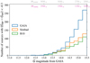 |
Fig. B.1. Number distributions of the G magnitudes of sources in the Gaia, Simbad, and B10 (Bonanos et al. 2010) catalogs that have a Gaia color of GBP − GRP < −0.3. Indicated at the top axis are the apparent G magnitudes from Gaia that stars of a certain mass have at the ZAMS and TAMS at the distance of the SMC, and an extinction of AV = 0.35. |
The discussion in the paragraph above assumes that the Gaia catalog is complete for stars that would be shown in our HRDs. To test the completeness of the Gaia catalog, we compared it with the UBVI catalog of Zaritsky et al. (2002). For different magnitude bins, we show the ratio of the number of stars in the Gaia catalog to the number of stars in the Zaritsky et al. (2002) catalog (Fig B.2). For the Gaia sources included in this figure, we made a color cut of GBP − GRP < 0.55 to exclude red sources. Empirically, we find that sources with Gaia color GBP − GRP < 0.55 have a color B − V < 0.35 in the Zaritsky et al. (2002) catalog. For the Zaritsky et al. (2002) sources we therefore applied a color cut of B − V < 0.35 instead of 0.55. In Fig. B.2 we compare G to V magnitudes, but we find that they do not differ by more than ∼0.03 for the vast majority of the sources that we consider. The error bars are derived from the number of sources in a bin (N):  . Figure B.2 shows that the ratio of sources in both catalogs is very close to one. For the brightest sources, there is some scatter, which is explained by the low number of sources in each bin. This result implies that Gaia is highly complete. The same has been implied by the fact the we find a Gaia counterpart for nearly all the B10 sources (Sect. 2). This good performance reflects the fact that as discussed by Arenou et al. (2018), Gaia is essentially complete except in regions of very high stellar density, such as exist near the centers of globular clusters, or for close visual binaries.
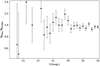 |
Fig. B.2. Ratio of sources in the Gaia and Zaritsky et al. (2002) catalogs in different magnitude bins. |
Finally, we quantitatively investigated the apparent discrepancy in the number of O stars in the SMC predicted by Massey (2010) and by our method based on the B10 catalog. The B10 catalog contains 259 O stars. For a typical completeness of 40% (Fig. B.1), we would expect about 600 O stars in total. In their Table 1, Massey (2010) list a much larger number of 2800 O stars above 20 M⊙ alone. To look for clues, we cross-correlated Table 8b from Massey (2002) with the B10 catalog. We again used cds-xmatch and cross-correlated within 3″. This Table 8b from Massey (2002) contains 2671 blue stars (of which 1901 rather than 2800 have a listed Teff > 30 kK, required to be considered O stars). For the 2671 blue stars from Massey (2002) (with median V = 14.84), we find 841 matches. This is slightly worse than but comparable to the ∼40% completeness we have around that G magnitude in Fig. B.1. Of the stars with a listed Teff > 30 kK that are also in B10, 191 of 513 (37%) have the expected O type in B10. The rest have a later type, predominantly B. A simple estimate then gives a number of 0.37 ⋅ 1901 = 703 of the Massey O stars to be O stars in reality. This number agrees well with our expected number of about 600. We note that this comparison likely suffers from biases that could go in both directions (e.g., O stars possibly being more likely to end up in the B10 catalog than later-type stars, or the adopted cut at Mbol = −7 for the sources included in Massey 2002’s Table 8b).
B.2. Extinction
We start this section by providing a few in-depth remarks on how we calculate the extinction. We did find unphysical negative extinction values, but only for less than 1% of the sources, with AV = −0.13 in the worst case. We consider this result to be comforting. Conversely, we also find very high extinction values of 1.95 ≤ AV ≤ 5.5 for 22 cases. Inspection shows that 14 of these make up the entire upper end of the 14 highest G magnitudes (i.e., they are not bright). By far the most of these (apparently) very high extinction sources have uncertain spectral types, for example, B1-5 III. The earliest spectral type is O9. Therefore they appear to be unable to make up part of the missing early O stars discussed in Sect. 4.3. We deem it most likely that these sources are chance alignments of cool (i.e., relatively red) dim sources. Our motivation for this is as follows. About half of the sources from the Gaia – B10 cross-match have more that one match, that is, a chance alignment, with a typically cool, dim source. Also, we find no Gaia match for 20 B10 sources. Because the probabilities to have or lack a chance alignment are about equal, we would also expect 20 B10 sources without their true match but only chance alignments. The number of 22 likely chance alignments fits this expected number of 20 surprisingly well. In Figs. 6 and B.6, if we encountered a value of AV > 1.95, we therefore assume our standard value of AV = 0.35 instead.
We also briefly considered extinction toward our sources from a theoretical side. As discussed in Sect. 6.2, we took a closer look at the simulations of Geen et al. (2018). In this work, a 10 000 M⊙ gas cloud was simulated, including the formation of stars and their feedback. In Fig. B.3 we show the fraction of gas that has been converted into stars. We compared the whole ensemble of stars to the subset of stars that would most likely be visible. The latter was defined as those with an extinction of AV ≤ 5 toward their line of sight. The extinction was obtained from the hydrogen column density in the simulation using the relation AV = NH/(1.8 ⋅ 1021cm−2) mag (Lombardi et al. 2014). It shows that immediately after formation, most of the model stars have an extinction of AV > 5, most likely preventing them from being included in observational studies in the optical.
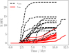 |
Fig. B.3. Star formation efficiency, defined as SFE = Mstars/(Mstars + Mgas), as a function of time in a simulation of Geen et al. (2018). Dashed lines indicate the total fraction of mass that is converted into stars, red is the same fraction, but with the requirement that the star has an extinction lower than AV = 5. The different dashed and red lines represent simulations with different initial conditions. |
B.3. Hertzsprung-Russell diagrams
The first test HRD that we provide (as discussed in Sect. 3) is Fig. B.5. It compares our result to the results of studies in the VSS sample. Wenn a source within 1″ is in the VSS sample, we point an arrow to its literature values. We note that the outlier around log(LVSS/L⊙)−log(LB10/L⊙) = 0.8 with log(LB10/L⊙) ≈ 5.05 is classified as a B3 star in the B10 catalog, but as an O9 star in Mokiem et al. (2006). If the latter type is assumed, the luminosity difference is only 0.1 dex. In general, we find that temperatures and luminosities we derived for the B10 sources agree reasonably well with the HRD positions predicted by the studies in the VSS sample. In this HRD, we do not include the yellow supergiants from Neugent et al. (2010) because those temperatures are based on photometry and not atmosphere analysis. The stars from Castro et al. (2018) are also omitted because of the low quality of their input data (this is the RIOTS4 survey of Lamb et al. 2016, aimed at SMC field stars). It did not allow the analysis of metal lines. Therefore they had to resort to the ionization balance of hydrogen and helium, which could not reliably constrain Teff in all corners of the HRD. Moreover, they stated that the surface gravities of the brightest stars are unreliable, causing stars in the spectroscopic HRD to artificially move up in luminosity. We note that these authors reported that there were only few massive stars close to the ZAMS in this sample from the RIOTS4 survey, as they also noted in their earlier study in the Milky Way (Castro et al. 2014).
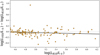 |
Fig. B.4. Same as Fig. 2, but here the B10 luminisoties are calculated differently. Instead of assuming a constant visual extinction of AV = 0.35, AV is calculated for each star individually. |
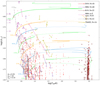 |
Fig. B.5. Same as Fig. 5, but the arrows point at temperatures and luminosities of objects in various spectroscopic studies. D19 stands for Dufton et al. (2019), H08 for Hunter et al. (2008b), R19 for Ramachandran et al. (2019), M06 for Mokiem et al. (2006), B13 for Bouret et al. (2013), and T04/05 for Trundle et al. (2004) and Trundle et al. (2004). |
Throughout the paper, we assume a constant extinction value of AV = 0.35. As a test, we also calculated the extinction for each source individually (as explained in Sect. 3.1 ; see also the AV distribution in Fig. 6). This results in slightly more luminous sources in the HRD (Fig. B.6), but the difference is not large enough to affect our conclusions.
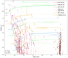 |
Fig. B.6. Same as Fig. B.5, but here the extinction is calculated per star, rather than assuming a constant value of AV = 0.35. |
We provide two more HRDs to test the robustness of our results (discussed in Sect. 3). In one (Fig. B.7), we have determined the temperatures and luminosities using the spectral type – temperature relations of Pecaut & Mamajek (2013) instead of those presented in Table A.1. This results in slightly different individual values, but a population that again has almost the same shape as the one shown in Fig. 5. In the other test, Fig. B.8, the source catalog of the spectral types is Simbad instead of B10. The main motivation for making this Simbad HRD is
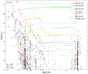 |
Fig. B.7. Same as Fig. B.5, but with spectral type – Teff relations of Pecaut & Mamajek (2013) instead of those from Table A.1. |
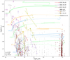 |
Fig. B.8. Same as Fig. B.5, but with with spectral types taken fron Simbad instead of Bonanos et al. (2010). It contains 1095 sources instead of the 780 that are in our B10 sample HRD. |
Adopted spectral type-temperature relation for SMC stars with different spectral types and luminosity classes.
to test whether the apparent lack of young and bright massive stars might result from a biased input catalog. The resulting HRD (Fig. B.8) contains more sources (1023 instead of 780), but it has the same features as the HRD shown in Fig. 5. This suggests that our results are robust from drawing on a (slightly) different compendium of observational types.
The next HRD in this appendix is Fig. B.9, which highlights the regions that were found to be completely devoid of stars in other studies. This is discussed in Sect. 6.1.3. These studies are Castro et al. (2014) and Holgado et al. (2020), in which luminous Milky Way stars were spectroscopically analyzed. We have drawn the lines in our figure such that the distance in log(Teff/K) from the ZAMS to the edge of the void is the same as in these studies. The sample of Holgado et al. (2020) contains 285 stars (O-types only) with evolutionary masses in excess of 25 M⊙. The exact number is not clear for the HRD of Castro et al. (2014), where shading indicates the number density of stars, but it can be expected to be ∼100. Figure B.9 shows that these voids extend to temperatures comparable to the half-MS temperature. Inspection of the Brott et al. (2011) models shows that this holds for Milky Way metallicity. This shows that in these subsamples with about (a few) 100 stars, fewer than a handful of stars are in the first half of their MS lifetime according to the tracks. In the evolutionary mass interval of 32 − 50 M⊙, this number reaches zero. Finally, we show Fig. B.10, which highlights observed stars with emission features (discussed in Sect. 4.1) and (X-ray) binaries (discussed in Sect. 2.1).
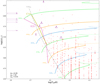 |
Fig. B.9. Same as Fig. 5, but here we indicate the regions that were found to be devoid of stars in earlier studies. To be more precise, there are no stars at the hot side of these lines in those studies. C14 means Castro et al. (2014), and H20 means Holgado et al. (2020). We note that we only show the hot stars in this diagram. |
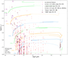 |
Fig. B.10. Hertzsprung-Russell diagram where we highlight sources with the label “binary” or “XRB” (X-ray binary) in Bonanos et al. (2010) (B10), and sources that show emission features. Emission features can be indicated by spectral type information in the B10 catalog, or by an infrared color larger than J − [3.6] = 0.5 mag in B10. This figure contains slightly fewer sources than for example Fig. 5 because it only shows those that have both a known J and [3.6] magnitude. |
Appendix C: Calculation of star formation rate and ionizing radiation emission
C.1. Star formation rate
Here we describe how we have estimated the SFR discussed in Sect. 3.1. For this we used the IMF of Kroupa (2001). There, the exponent Γ of the IMF, ξ(log M) = dN/d log M ∝ MΓ, with M in solar units, has the following values in different mass intervals:
-
Γ = +0.7, for 0.01 ≤ M < 0.08
-
Γ = −0.3, for 0.08 ≤ M < 0.50
-
Γ = −1.3, for 0.50 ≤ M.
However, we are not interested in the number of stars, but in the yearly amount of mass that is converted into stars. Therefore the distribution has to be multiplied by a factor M because more massive stars contain more mass. We consider ξmass in stars(log M) = dN/d log M ∝ Ma. Thus,
-
a = +1.7, for 0.01 ≤ M < 0.08
-
a = +0.7, for 0.08 ≤ M < 0.50
-
a = −0.3, for 0.50 ≤ M.
Figure C.1 shows the resulting stellar mass distribution as a function of birth mass. Assuming an upper mass limit (this limit is more important now because the most massive stars contribute more in mass than in numbers) of 150 M⊙, 13.7% of the mass converted into stars ends up in stars born with 18 M⊙ or more. Therefore fM > 18 M⊙ = 0.137. This corresponds to the area of the hatched region divided by the total area below the curve in Fig. C.1. This number changes slightly if, for example, 100 M⊙ (11.9%) or 250 M⊙ (15.5%) is chosen as upper mass limit.
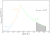 |
Fig. C.1. Distribution of stellar mass as a function of birth mass, upon star formation. Above the curve, we show the numbers that indicate the slope of the mass distribution. The hatched region is the region where stars have a mass between 18 M⊙ and the assumed upper mass limit of 150 M⊙. |
Then, we proceed to estimate the SFR for CSF in the following steps. Clearly, the CSF scenario does not match the
inferred age distribution, but we use it as a starting point in this estimation.
-
We consider the orange line in the bottom right panel of Fig. 9. It shows that to derive the amount of stars with M > 18 M⊙ that is in the HRD with the B10 sources (Fig. 5), they need to be produced at a rate of about 50 Myr−1 (after some million years, the curve drops because stars start to die).
-
We find that these stars have an average mass of ∼25 M⊙. This results in approximately 1250 M⊙ Myr−1 or 0.00125 M⊙ yr−1.
-
The completeness of the stars above the 18 M⊙ track should be about 40 − 50% (Sect. 2.2). This doubles the inferred SFR to ∼0.0025 M⊙ yr−1 in the considered mass range.
-
Above, we found that fM > 18 M⊙ = 0.137. Integrated over the entire mass spectrum, the SFR therefore equals 0.0025 M⊙ yr−1/0.137 = 0.018 M⊙ yr−1.
A typical literature value for the SFR in the SMC at recent times is ∼0.05 M⊙ yr−1 (Sect. 3.1). This value is significantly higher than the value we just derived for a CSF scenario. If the SFR is not constant, as is the case for SFH2 and SFH3, it is necessary (to explain the observed number of M > 18 M⊙ stars) that 7 − 10 Myr ago, the SFR was about a factor three higher than the SFR in the CSF scenario (bottom right panel in Fig. 9). At that point in time, we therefore estimate that the SFR was about 0.045 M⊙ yr−1. We note that this argument works the same way if, instead of a drop in the SFR, young stars are not observed due to biases.
We also investigated how much steeper the IMF should be to derive the typical literature value of ∼0.05 M⊙ yr−1 For this, we changed the exponent a in the highest mass interval (green line in Fig. C.1). For a = −0.6 (i.e., a slightly steeper IMF of Γ − 1.6) we find fM > 18M⊙ = 0.049, which then results in the literature SFR of 0.05 M⊙ yr−1. While tuning the IMF can fix the lack of bright stars, however, it does not fix the lack of young stars.
C.2. Ionizing radiation
We considered POWR models7[SMC grid OB I of][see also Todt et al. 2015]Hainich19 and fit their log Q, which is the ionizing photon production rate. We did this for H I, He I, and He II using the following fit formula:
 (C.1)
(C.1)
Here, log Teff m4 is defined as log(Teff/K)−4, which allowed a better fit than log(Teff/K). The fitting constants that we find for H I, He I, and He II are tabulated in Table C.1. The POWR grid extends to 50 kK. Because we are hesitant to extrapolate outside this range, we treated hotter stars as if their Teff were 50 kK. The observed population has only one star above Teff = 50 kK, at 51.7 kK. However, the synthetic population shown in Fig. 10 contains more stars above Teff = 50 kK, and even hotter stars. It is therefore possible that we underestimate QHe II in the synthetic population. This would strengthen our conclusions that QHe II is much lower in the observed population than in the synthetic population. This limit of 50 kK is expected to play less of a role for the total of QH I and QHe I, because these are not dominated by the ∼10 hottest stars.
Values used for the log Q fit.
In Table C.1 we show the ionizing photon production rate of the 780 stars in the observed population (Fig. 5) and the synthetic population (Fig. 10). Because the brightest, hottest stars are expected to be fairly complete (about 80%), we do not expect the real values to be much higher in practice.
POWR models of WR stars (all have log(L/L⊙) = 5.3) hotter than 50 kK emit log QH I = 1049.15. Above this temperature value, this number changes only by about 0.02 dex for different temperatures, transformed radii, and hydrogen surface abundances. We can accordingly assume for the SMC WR stars analyzed by Hainich et al. (2015) and Shenar et al. (2016) that they emit QH I = 1049.15 − 5.3 = 1043.85 photons per second per unit of solar luminosity. Summing the luminosities of all these SMC WR stars yields a total luminosity of log(L/L⊙) = 7.17. Their total rate of HI ionizing photon production is then QH I = 1043.85 + 7.17 = 1051.02. For He I we adopt QH I = 1048.95 − 5.3 = 1043.85 photons per second per unit of solar luminosity as a representative value after looking up POWR models. This leads to QHe I = 1050.82. Similarly, for He II, we obtain QHe II = 1046.55 − 5.3 = 1041.25 photons per second per unit of solar luminosity, making a total of QHe II = 1048.42.
We summed the H I ionizing emission of WR and non-WR stars. This results in QH I = 3 ⋅ 1051. QHe I, tot is dominated by WR stars, although in the synthetic population the contribution of MS stars is comparable. On the other hand, QHe I is completely dominated by the WR stars in any case by some orders of magnitude.
Appendix D: Positions and motions of sources
Below, we briefly investigate whether the inferred drop of the SFR (Sect. 4.3) would have needed to take place over the entire SMC, or if the stars younger than 10 Myr can come from only a few birth places. For this, we considered the Gaia proper motions of the sources in the B10 data set that are shown in Fig. 9, that is, those with evolutionary masses in excess of 18 M⊙ and ages younger than 10 Myr. For each of these sources, we calculated their proper motion relative to the SMC by subtracting an SMC bulk motion of μra = 0.695 mas yr−1 and μra = −1.206 mas yr−1 (Yang et al. 2019) from their Gaia proper motions. Then, we used their inferred age (Sect. 4.3) to estimate how far they have traveled during their lifetime so far, in terms of both right ascension and declination. The bottom left panel of Fig. D.1 shows the distribution of the absolute values of how far the sources traveled in both directions. In right ascension, the median is 0.82 degrees. In declination, the median is 0.13 degrees. The main reason for this difference is that the SMC, with its declination of about −72.5 degrees, is close to the south pole.
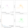 |
Fig. D.1. Diagrams showing positions and motions of sources in the Small Magellanic Cloud. The top left panel shows the positions of the sources that are in the VSS. The bottom left panel shows the distribution of the integrated motion relative to the SMC of B10 sources (that are above the 18 M⊙ track in Fig. 5) since their birth (see text). The top and bottom right panel show the positions of these B10 sources now and integrated to their their moment of birth in the SMC, respectively. |
We can compare this with motions in the line-of-sight direction. Evans & Howarth (2008) provided radial velocities of 2045 2dF sources (about half of the sample). The value that they find for the radial velocity dispersion is ∼30 km s−1. For source with this velocity and a typical age of 7 Myr (Fig. 9), this indicates a typical lifetime travel distance of about 200 pc. This distance would correspond to a projected angular distance of 0.17 degrees in the declination direction. This shows that we obtain similar results from the proper motions and the radial velocity dispersion. For both methods, the lifetime travel distances are likely amplified by the errors (observational errors, and for the radial velocities, reflex motion due to binary companions). The real travel distances within the SMC would therefore most likely be smaller than the values mentioned above.
The top right panel of Fig. D.1 shows the current position of the sources that are displayed in Fig. 9. The SMC has an angular size on the order of a few (in declination) by ten (in right ascension) degrees. This is more than a factor ten larger than the typical angular distance that these sources have traveled with respect to the SMC during their lifetime. During their lifetimes, these sources therefore cannot have traveled through a significant part of the SMC. Combining this with the fact that the B10 sources above 18 M⊙ are currently spread out all over the SMC (top right panel in Fig. D.1), it is implied that the hypothetical halt in star formation would have had to take place over the entire SMC at roughly the same time.
In the bottom right panel of Fig. D.1, we give an impression of the birth locations within the SMC of the sources that are displayed in Fig. 9. Similar to what is described above, we used relative proper motions and inferred ages of these sources to trace back where they resided in the SMC when they were born. This figure implies that at the moment of birth, these sources were also spread out over the SMC. The angular scale of the plot is the same as in the top right panel of the figure. This strengthens our original assumption that the stars above 18 M⊙ originate from a multitude of birth places in the SMC, rather than being born in only a few sites. For reference, we also show the positions of the sources in the VSS sample in the top left panel of Fig. D.1.
All Tables
Adopted spectral type-temperature relation for SMC stars with different spectral types and luminosity classes.
All Figures
|
Fig. 1. Derived relations of spectral types and effective temperatures (crosses) for different luminosity classes (LCs). The solid gray line shows the relation for Galactic dwarf stars (P13; Pecaut & Mamajek 2013). |
| In the text | |
|
Fig. 2. Difference between the logarithm of the luminosities reported in the various spectroscopic studies (VSS) sample and those derived by our method using spectral types of B10 as a function of log(LB10/L⊙). Each dot represents an individual source. The dotted line shows where LB10 = LVSS; the solid line is a linear fit to the scatter points. |
| In the text | |
|
Fig. 3. Hertzsprung-Russell diagram of bright SMC sources constructed with Gaia photometry. Black markers indicate sources from the Gaia sample. The smaller red markers are sources in the B10 sample. Therefore, red points with black edges (all but one of the red points, see Appendix A) are sources that are listed in both samples. We count the number of sources that are hotter than 103.8 K for both samples in different luminosity intervals. The numbers are displayed on the left side of the plot. The luminosity intervals are indicated by dashed blue lines. For completeness, we also show the cool sources with crosses. |
| In the text | |
|
Fig. 4. Correlation between the luminosity of sources as calculated using their Gaia color and magnitude (Lphot) and the luminosity of the same source derived in various spectroscopic studies (VSS) or its luminosity based on the temperature derived from the spectral type listed in B10. |
| In the text | |
|
Fig. 5. Hertzsprung-Russell diagram of luminous stars in the SMC. Red dots represent sources from the B10 data set. Open dark red squares are red supergiants from Davies et al. (2018), where the Teff is obtained using relations from Tabernero et al. (2018). We show the Wolf-Rayet stars (Hainich et al. 2015; Shenar et al. 2016, 2017) labeled with a ‘W’ and their identifying number. Whe they have an O-star companion that is brighter in the V-band, we show this instead (indicated by ‘(O)’). We also show evolutionary tracks of Schootemeijer et al. (2019) with a semiconvection parameter of αsc = 10, and an overshooting parameter of αov = 0.33. Solid lines indicate hydrogen- and helium-core burning phases; dashed lines indicate the in between phase. The dash-dotted gray line shows the location of these models halfway through their main-sequence (MS) lifetime, tMS. |
| In the text | |
|
Fig. 6. Distribution of the visual extinction AV in the B10 sample when measured for each source individually. We also show the AV distribution of the subset for which we derive a luminosity higher than log(L/L⊙) = 5.5, and the subset of stars with an ‘e’ label in the B10 data set. |
| In the text | |
|
Fig. 7. Diagram of the cumulative distribution of the ionizing photon production rate Q. The stars in this cumulative distribution are sorted from a high to low Q. |
| In the text | |
|
Fig. 8. Hertzsprung-Russell diagram showing the same SMC objects as Fig. 5, indicating which stars are considered as He-burning stars with initial masses between 18 and 29 M⊙. The tracks are from the extended grid of Schootemeijer et al. (2019). |
| In the text | |
|
Fig. 9. Fractional age (bottom left) and absolute age (bottom right) distribution of the number of stars that are above the 18 M⊙ track (referred to as N18+) in Fig. 5. The colored distributions are theoretical predictions for CSF, and two other star formation histories (SFH2 and SFH3) where young stars have a lower probability (top right panel). The gray line indicates the distribution that we derived using observations. |
| In the text | |
|
Fig. 10. Same as Fig. 5, except that it contains randomly drawn synthetic stars (purple crosses) and that the x-axis range does not extend to the temperature regime of red stars. The dashed lines separate the temperature ranges covered by different spectral types of luminosity class V, according to our spectral type-temperature relation (Sect. 2.1). |
| In the text | |
|
Fig. 11. Diagrams showing the high end of the distribution of luminosities that we derived for sources in the Bonanos et al. (2010) data set. Left is the uncorrected distribution. Right is the distribution corrected for the completeness of the B10 data set using Gaia data. For comparison, we show the theoretical values (diamonds) for different star formation history scenarios. We also show the number distributions when the brightest source in the WR star system is taken out. |
| In the text | |
|
Fig. B.1. Number distributions of the G magnitudes of sources in the Gaia, Simbad, and B10 (Bonanos et al. 2010) catalogs that have a Gaia color of GBP − GRP < −0.3. Indicated at the top axis are the apparent G magnitudes from Gaia that stars of a certain mass have at the ZAMS and TAMS at the distance of the SMC, and an extinction of AV = 0.35. |
| In the text | |
|
Fig. B.2. Ratio of sources in the Gaia and Zaritsky et al. (2002) catalogs in different magnitude bins. |
| In the text | |
|
Fig. B.3. Star formation efficiency, defined as SFE = Mstars/(Mstars + Mgas), as a function of time in a simulation of Geen et al. (2018). Dashed lines indicate the total fraction of mass that is converted into stars, red is the same fraction, but with the requirement that the star has an extinction lower than AV = 5. The different dashed and red lines represent simulations with different initial conditions. |
| In the text | |
|
Fig. B.4. Same as Fig. 2, but here the B10 luminisoties are calculated differently. Instead of assuming a constant visual extinction of AV = 0.35, AV is calculated for each star individually. |
| In the text | |
|
Fig. B.5. Same as Fig. 5, but the arrows point at temperatures and luminosities of objects in various spectroscopic studies. D19 stands for Dufton et al. (2019), H08 for Hunter et al. (2008b), R19 for Ramachandran et al. (2019), M06 for Mokiem et al. (2006), B13 for Bouret et al. (2013), and T04/05 for Trundle et al. (2004) and Trundle et al. (2004). |
| In the text | |
|
Fig. B.6. Same as Fig. B.5, but here the extinction is calculated per star, rather than assuming a constant value of AV = 0.35. |
| In the text | |
|
Fig. B.7. Same as Fig. B.5, but with spectral type – Teff relations of Pecaut & Mamajek (2013) instead of those from Table A.1. |
| In the text | |
|
Fig. B.8. Same as Fig. B.5, but with with spectral types taken fron Simbad instead of Bonanos et al. (2010). It contains 1095 sources instead of the 780 that are in our B10 sample HRD. |
| In the text | |
|
Fig. B.9. Same as Fig. 5, but here we indicate the regions that were found to be devoid of stars in earlier studies. To be more precise, there are no stars at the hot side of these lines in those studies. C14 means Castro et al. (2014), and H20 means Holgado et al. (2020). We note that we only show the hot stars in this diagram. |
| In the text | |
|
Fig. B.10. Hertzsprung-Russell diagram where we highlight sources with the label “binary” or “XRB” (X-ray binary) in Bonanos et al. (2010) (B10), and sources that show emission features. Emission features can be indicated by spectral type information in the B10 catalog, or by an infrared color larger than J − [3.6] = 0.5 mag in B10. This figure contains slightly fewer sources than for example Fig. 5 because it only shows those that have both a known J and [3.6] magnitude. |
| In the text | |
|
Fig. C.1. Distribution of stellar mass as a function of birth mass, upon star formation. Above the curve, we show the numbers that indicate the slope of the mass distribution. The hatched region is the region where stars have a mass between 18 M⊙ and the assumed upper mass limit of 150 M⊙. |
| In the text | |
|
Fig. D.1. Diagrams showing positions and motions of sources in the Small Magellanic Cloud. The top left panel shows the positions of the sources that are in the VSS. The bottom left panel shows the distribution of the integrated motion relative to the SMC of B10 sources (that are above the 18 M⊙ track in Fig. 5) since their birth (see text). The top and bottom right panel show the positions of these B10 sources now and integrated to their their moment of birth in the SMC, respectively. |
| In the text | |
Current usage metrics show cumulative count of Article Views (full-text article views including HTML views, PDF and ePub downloads, according to the available data) and Abstracts Views on Vision4Press platform.
Data correspond to usage on the plateform after 2015. The current usage metrics is available 48-96 hours after online publication and is updated daily on week days.
Initial download of the metrics may take a while.