It has to be cool: Supergiant progenitors of binary black hole mergers from common-envelope evolution

Jakub Klencki; Gijs Nelemans; Alina G. Istrate; Martyna Chruslinska

doi:10.1051/0004-6361/202038707

Home

All issues

Volume 645 (January 2021)

A&A, 645 (2021) A54

Full HTML

Free Access

Issue		A&A Volume 645, January 2021


Article Number		A54
Number of page(s)		27
Section		Stellar structure and evolution
DOI		https://doi.org/10.1051/0004-6361/202038707
Published online		08 January 2021

A&A 645, A54 (2021)

It has to be cool: Supergiant progenitors of binary black hole mergers from common-envelope evolution

Jakub Klencki¹, Gijs Nelemans¹^,2^,3, Alina G. Istrate¹ and Martyna Chruslinska¹

¹ Department of Astrophysics/IMAPP, Radboud University, PO Box 9010, 6500 GL Nijmegen, The Netherlands
e-mail: j.klencki@astro.ru.nl
² Institute of Astronomy, KU Leuven, Celestijnenlaan 200D, 3001 Leuven, Belgium
³ SRON, Netherlands Institute for Space Research, Sorbonnelaan 2, 3584 CA Utrecht, The Netherlands

Received: 19 June 2020
Accepted: 27 September 2020

Abstract

Common-envelope (CE) evolution in massive binary systems is thought to be one of the most promising channels for the formation of compact binary mergers. In the case of merging binary black holes (BBHs), the essential CE phase takes place at a stage when the first BH is already formed and the companion star expands as a supergiant. We aim to decipher the kinds of BH binaries with supergiant companions that could potentially evolve through and survive a CE phase. To this end, we compute envelope binding energies from detailed massive stellar models at different evolutionary stages and metallicities. We make multiple physically extreme choices of assumptions that favor easier CE ejection as well as account for recent advancements in mass-transfer stability criteria. We find that even with the most optimistic assumptions, a successful CE ejection in BH binaries is only possible if the donor is a massive convective-envelope giant, namely a red supergiant (RSG). The same is true for neutron-star binaries with massive companions. In other words, pre-CE progenitors of BBH mergers are BH binaries with RSG companions. We find that because of its influence on the radial expansion of massive giants, metallicity has an indirect but a very strong effect on the chemical profile, density structure, and the binding energies of RSG envelopes. Our results suggest that merger rates from population-synthesis models could be severely overestimated, especially at low metallicity. Additionally, the lack of observed RSGs with luminosities above log(L/L_⊙) ≈ 5.6 − 5.8, corresponding to stars with M ≳ 40 M_⊙, puts into question the viability of the CE channel for the formation of the most massive BBH mergers. Either such RSGs elude detection due to very short lifetimes, or they do not exist and the CE channel can only produce BBH systems with total mass ≲50 M_⊙. Finally, we discuss an alternative CE scenario in which a partial envelope ejection is followed by a phase of possibly long and stable mass transfer.

Key words: stars: evolution / binaries: close / stars: black holes / gravitational waves / supergiants

© ESO 2021

1. Introduction

Since the discovery of the first gravitational wave (GW) signal from a binary black hole (BBH) coalescence by the Advanced LIGO Interferometer in September 2015 (GW150914, Abbott et al. 2016), the LIGO/Virgo Collaboration has reported the detection of nine further BBH mergers by the end of its second observing run O2 (Abbott et al. 2019). The third observing run O3 has been concluded and a large number of publicly issued alerts is an indication that a few tens of additional detections of BBH mergers will soon be announced, including the recently published discoveries of GW190412 (The LIGO Scientific Collaboration & the Virgo Collaboration 2020a), GW190814 (being either a BBH or a BH-neutron star(NS) merger; Abbott et al. 2020), and GW190521 (The LIGO Scientific Collaboration & the Virgo Collaboration 2020b). With the growing population of BBHs, the discussion of possible formation scenarios of compact binary mergers is as lively as ever. A large number of channels have been put forward, especially in the case of BBHs. These include but are not limited to the formation from isolated binaries through common-envelope (CE) evolution (Dominik et al. 2012; Mennekens & Vanbeveren 2014; Belczynski et al. 2016; Eldridge & Stanway 2016; Klencki et al. 2018; Mapelli & Giacobbo 2018; Kruckow et al. 2018; Breivik et al. 2020) or in a chemically homogeneous evolution regime (Mandel & de Mink 2016; de Mink & Mandel 2016; Marchant et al. 2016), dynamical formation in globular clusters (Rodriguez et al. 2016; Askar et al. 2017; Samsing 2018), in nuclear clusters (Arca-Sedda & Gualandris 2018; Fragione & Kocsis 2019), or in disks of active galactic nuclei (AGNs; Antonini & Rasio 2016; Stone et al. 2017; McKernan et al. 2018), as well as formation channels involving triple (Antonini et al. 2017) or quadruple stellar systems (Fragione et al. 2019). So far, it has not been possible to distinguish between various channels based on the gravitational wave information alone. In particular, the promising method of distinguishing between dynamical and isolated binary formation based on the BBH spin-orbit misalignment distribution (Farr et al. 2017, 2018) is hindered by our lack of knowledge of the natal black hole (BH) spins and, to a lesser extend, the possibility of BH natal kicks changing the spin orientation (O’Shaughnessy et al. 2017; Gerosa et al. 2018; Belczynski et al. 2020; Bavera et al. 2020). As a result, the contribution of various channels to the entire population of BBH mergers is usually estimated on theoretical grounds (Abadie et al. 2010; Barack et al. 2019). The CE evolution channel is sometimes considered to be especially promising thanks to its potential to produce a relatively high merger rate of BBHs compared to other channels, although any rate prediction from theoretical population models are highly uncertain.

The essential stage in the CE evolution channel is a dynamically unstable phase of mass transfer that leads to rapid spiraling in of the companion object inside the shared envelope originating from the giant donor star (Paczynski 1976; Webbink 1984; Iben & Livio 1993; Podsiadlowski 2001; Ivanova et al. 2013a). The drag force is thought to cause a dramatic shrinkage of the binary separation, and the dissipated orbital energy to lead to an ejection of the CE (under the right circumstances) or a merger otherwise. The huge range in both timescales and length scales involved in this complex process makes hydrodynamic simulations challenging (e.g., Ricker & Taam 2012; Passy et al. 2012; Nandez & Ivanova 2016; MacLeod et al. 2017; Fragos et al. 2019). As a result, the exact outcome of the CE phase is difficult to predict. However, there is a substantial amount of evidence for significant orbital shrinkage in progenitors of various short-period systems such as cataclysmic variables (e.g., Paczynski 1976; Meyer & Meyer-Hofmeister 1979), binary white dwarfs (e.g. Han 1998; Nelemans et al. 2000, 2001), or binary neutron stars (BNSs; e.g., van den Heuvel 1994; Tauris & van den Heuvel 2006; Chruslinska et al. 2018; Vigna-Gómez et al. 2020), which cannot be explained without invoking a mechanism such as the CE phase.

In the case of more massive stars, which are the progenitors of stellar BHs (≳20 M_⊙), such observational support is more difficult to find and comes mainly from the population of short-period (< 1 day) X-ray binaries with stellar BH accretors and low-mass (≲1 M_⊙) donors (BH-LMXBs; Casares & Jonker 2014), which are believed to have formed through CE evolution (Portegies Zwart et al. 1997; Kalogera 1999). High-mass X-ray binaries hosting stellar BHs and Wolf-Rayet (WR) companions in short-period orbits of a few hours up to two days, such as Cygnus X-3, IC10 X-1, and NGC300X-1, may also be products of the CE evolution (Lommen et al. 2005; Carpano et al. 2007), although whether or not they could originate from stable mass transfer evolution instead is debated (van den Heuvel et al. 2017). Notably, such systems could be the immediate progenitors of merging BBH or BH–NS systems (Bulik et al. 2011; Belczynski et al. 2013). On top of that, hydrodynamic simulations of the CE phase are particularly challenging in the case of massive stars (see Ricker et al. 2019, for details) and most of the hitherto results have been limited to low-mass giants, which are WD progenitors.

Motivated by the LIGO discoveries of the BBH mergers GW150914 and GW151226, Kruckow et al. (2016) analyzed the prospect of successful CE evolution in binaries of stellar BHs and massive companions (i.e., potential BBH progenitors) by considering the energy balance between the envelope binding energy and the available energy sources (van den Heuvel 1976; Webbink 1984; Ivanova et al. 2013a). They concluded that for the right binary parameters, the CE evolution channel may indeed operate for massive stars in a similar way to low- and intermediate-mass donors, and that it may produce BBH systems with individual BH masses all the way up to the lower edge of the pair-instability supernova (PISN) BH mass gap (at ∼45 − 55 M_⊙, e.g., Heger et al. 2003; Woosley 2017; Leung et al. 2019; Renzo et al. 2020, although the limit could perhaps be moved to higher masses within the uncertainty of the ¹²C(α, γ)¹⁶O reaction rate, Farmer et al. 2019).

Here, we extend the analysis of Kruckow et al. (2016) by additionally accounting for conditions necessary for the mass transfer to become dynamically unstable (i.e., for the occurrence of CE evolution). Such conditions can usually be formulated in the form of a threshold mass ratio, such that for mass ratios q = M_donor/M_accretor above a critical value q_crit the mass transfer becomes unstable, whereas for q < q_crit the CE evolution is avoided. Importantly, the mass ratio q plays a significant role in considerations of the CE energy budget: the lower the q (i.e., a more equal-mass system) the larger the energy input from orbital shrinkage, which makes it more likely to unbind the envelope and survive the CE phase (e.g., Fig. 6 of Kruckow et al. 2016). Recent studies of mass transfer stability from massive giants reveal that the mass transfer remains stable for a larger parameter space than previously thought, thus avoiding a CE evolution in the majority of cases (Woods & Ivanova 2011; Pavlovskii et al. 2017). It is therefore essential to consider realistic q_crit values when addressing the question of CE ejectability in BBH progenitors.

In Sect. 2 we describe the ingredients of our model: (a) detailed stellar models of massive giants for six metallicities between Z = 0.017 = Z_⊙ and Z = 0.00017 = 0.01 Z_⊙, (b) conditions for mass-transfer instability and the occurrence of CE evolution, and (c) the assumed contribution of various energy sources and sinks to the overall energy budget of the CE evolution. In Sect. 3 we present our calculated envelope binding energies, highlighting the substantial impact of outer convective envelopes. Furthermore, we compute the parameter space for successful CE ejections and explore the impact of various assumptions. Finally, we explore the predicted population of CE survivors in the Hertzprung-Russell (HR) diagram. We discuss various aspects of our findings in Sect. 4 and conclude in Sect. 5.

2. The model

2.1. Stellar models of massive giants

We use rotating single stellar models from Klencki et al. (2020) computed with the MESA stellar evolution code (Paxton et al. 2011, 2013, 2015, 2018, 2019). The use of single models unperturbed by previous binary interactions is a simplification because in most realistic scenarios the stellar companion in a BH binary is a mass gainer from a mass transfer phase that was initiated by the BH progenitor (also in the case of BBH merger progenitors, e.g., Belczynski et al. 2016). While this has become common practice, there is an important caveat to mention. We discuss this topic further in connection to those results that are likely the most sensitive to the assumption of single stellar models (see Sects. 3.4 and 4.1).

The tracks from Klencki et al. (2020) cover a range of masses from 10 to 80 M_⊙ and six metallicity values, Z = 0.017, 0.0068, 0.0034, 0.0017, 0.00068, and 0.00017 (or in fractions of the solar metallicity: 1.0, 0.4, 0.2, 0.1, 0.04, and 0.01 Z_⊙, where we assume Z_⊙ = 0.017 after Grevesse et al. 1996), with the initial rotation rate set to 40% of the critical value (Ω/Ω_crit = 0.4). We note that for higher initial rotation rates, massive stars of M ≳ 50 M_⊙ at very low metallicities were shown to evolve in a chemically homogeneous way (e.g., Marchant et al. 2017). Convection was modeled using the mixing-length theory (Böhm-Vitense 1958) with a mixing length of α_ML = 1.5 and following the Ledoux criteria for convection with a high efficiency of semiconvective mixing α_SC = 100. The models assume step overshooting above the hydrogen and helium burning cores with an overshooting length of 0.345 pressure scale heights (Brott et al. 2011). The wind mass-loss was modeled, following (Brott et al. 2011), as a combination of mass-loss recipes from Nieuwenhuijzen & de Jager (1990), Hamann et al. (1995), and Vink et al. (2001). Notably, the models from Klencki et al. (2020) were computed under a set of assumptions that maximizes the potential of massive stars to reach the sizes of red-supergiants and to develop deep outer convective envelopes: with no luminous blue variable (LBV) mass-loss above the Humphreys-Davidson limit and without preventing the formation of density inversions by the use of MLT++ in MESA (see Appendix A in Klencki et al. 2020). Such an approach allows us to explore the maximum potential parameter space for binary interactions in wide binaries and consequently the maximum parameter space for CE evolution. In the case of convective-envelope stars with initial masses ≳40 M_⊙ the true parameter space might be significantly smaller, as discussed in Sect. 4.2. We refer to Klencki et al. (2020) for a description of other physical ingredients of the models and zenodo¹ for the MESA input files. In Appendix B we demonstrate the models are numerically robust for the purposes of this work.

2.2. Conditions for mass-transfer instability

Mass transfer in a binary can become dynamically unstable when either the donor or the accretor (or both) expands too much in size with respect to its Roche-lobe. It was shown that if the timescale of mass transfer is short compared to the thermal timescale of the mass gainer then the accreting star could be driven out of thermal equilibrium and expand significantly (e.g., Benson 1970; Neo et al. 1977), filling its Roche-lobe and leading to the formation of a contact binary (Pols 1994; Wellstein et al. 2001) and potentially a CE evolution (de Mink et al. 2007; Marchant et al. 2016). Details of this process remain largely uncertain, partly because of the complicated gas dynamics in semi-detached binaries (Lubow & Shu 1975), poorly constrained specific entropy of the accreted material (Shu & Lubow 1981), and unknown efficiency of accretion by stars rotating near their breakup limit (Popham & Narayan 1991, see also discussion by de Mink et al. 2013).

However, the focus of this study is mass transfer in the case of compact-object accretors: stellar BHs or NSs². Based on X-ray binaries such as Cyg X-2 (King & Ritter 1999) and SS433 (Fabrika 2004), it is believed that unlike a stellar accretor, a BH or a NS can deal with very high mass transfer rates via jets and disk outflows which prevent the nonaccreted matter from piling up and eventually overflowing their Roche-lobes. For that reason, for the remainder of this section we discuss mass transfer instability due to an increasing Roche-lobe overflow by the donor star. As explained above, in the case of stellar accretors the mass transfer could be unstable in many more cases.

Donor stars with outer radiative envelopes (the case that dominates the parameter space) respond to mass loss by contraction on the adiabatic timescale (Hjellming & Webbink 1987; Soberman et al. 1997). In other words, they are characterized by a positive value of ζ_ad = (∂ log R/∂ log M)_ad. In such a case, the mass transfer can become unstable on the adiabatic timescale only when the size of the Roche-lobe is shrinking more quickly than the size of the radiative donor, which is possible if the mass ratio q = M_donor/M_accretor is higher than some critical value q_crit; rad. Traditionally, radiative-envelope post-main sequence(MS) giants were assumed to be described by ζ_ad ≈ 6.5, which corresponds to q_crit ≈ 3.5 − 4 (Tout et al. 1997; Hurley et al. 2002): a value that is often assumed (e.g., Schneider et al. 2015; van den Heuvel et al. 2017; Vigna-Gómez et al. 2018). Detailed models of mass transfer from intermediate-mass radiative-envelope donors (∼1–6 M_⊙) also found stability for mass ratios of up to about four (e.g., Tauris et al. 2000; Chen & Han 2002; Ivanova & Taam 2004). Observationally, the well-studied SS433 system, which consists of a Roche-lobe-filling A-type supergiant (∼12.3 M_⊙) and a stellar BH (∼4.3 M_⊙) in a 13.1 day period orbit (Hillwig & Gies 2008), is a likely case of stable mass transfer evolution that has already been ongoing for ∼10⁵ yr (with the likely initial value of q ≈ 3 − 4; King et al. 2000; Begelman et al. 2006; van den Heuvel et al. 2017). Notably, mass transfer from MS donors was found to be less stable with typical q_crit; MS ≈ 1.5 (de Mink et al. 2007).

A single value of ζ_ad across the entire mass and radius spectrum of post-MS stars is a serious simplification. Ge et al. (2015) computed adiabatic responses for a large grid of models (donor masses between 0.1 and 100 M_⊙), also taking into account the possibility of a delayed dynamical instability (Ge et al. 2010). The authors found that the value of ζ_ad = 6.5 and the critical mass ratio q_crit; rad between 3 and 5 could be a good approximation in the case of stars below 10 M_⊙. However, for more massive post-MS stars these latter authors find a higher q_crit; rad of at least 5, and even q_crit; rad > 10 for R > 300 R_⊙ (going up to extreme q_crit; rad > 20 for R > 1000 R_⊙).

Donor stars with outer convective envelopes on the other hand are expected to respond to mass loss by expanding on the adiabatic timescale. This makes the mass transfer from convective donors much more prone to dynamical instability than from radiative donors. Many authors have relied on condensed polytrope models of Hjellming & Webbink (1987) to obtain the value of ζ_ad for convective-envelope donors, which typically leads to critical mass ratios q_crit; conv of about 0.8.

It is important to take into account the caveats associated to the numbers cited above. The value of ζ_ad derived in the adiabatic approximation (e.g., Hjellming & Webbink 1987; Tout et al. 1997; Ge et al. 2015) is only valid for predicting the donor behavior if the outer envelope thermal timescale is much longer than the adiabatic timescale (i.e., the entropy profile can be considered constant). This is not necessarily the case for outer envelopes of massive stars with large radii. Woods & Ivanova (2011) showed that in the case of convective donors the thermal timescale in the outermost superadiabatic layer of the envelope (which forms on top of the convective zone) can become even smaller than the dynamical timescale. These latter authors found that thermal relaxation of such outer layers can effectively increase the stability of mass transfer (by up to a factor of ∼1.7 in q_crit; conv in the limited number of cases investigated by the authors)³. In the case of massive radiative donors, a qualitatively opposite effect of decreased stability is expected (see Sect. 4.1 of Ge et al. 2015), which is why the values of q_crit; rad > 10 are most likely overestimated.

The fact that thermal relaxations needs to be taken into account means that mass transfer stability from massive giants cannot be reliably predicted without detailed evolutionary calculations. Some such results are already available. Using 1D stellar codes with hydrodynamic terms to probe the rapid donor response, both Passy et al. (2012) and Pavlovskii & Ivanova (2015) found that the initial reaction of convective-envelope stars to mass loss is a slight contraction, contrary to what the adiabatic models predict. This increases the stability, in line with the conclusions of Woods & Ivanova (2011). Taking overflow through the outer Langrangian point as instability criteria, Pavlovskii & Ivanova (2015) obtained revised critical mass ratios for convective donors q_crit; conv = 1.5 − 2.2, computed for models of up to 50 M_⊙ in which the outer convective envelope is well developed (M_conv ≳ 0.3M_donor). For donors with less developed convective envelopes Pavlovskii & Ivanova (2015) obtain stability up to the highest mass ratio in their grid, q = 3.5, though they do not specify the exact M_conv value. In a recent work focused on intermediate-mass donors (M_donor between 1 and 8 M_⊙) Misra et al. (2020) found stable mass transfer evolution from convective-envelope donors for mass ratios up to q ∼ 2.

In the case of massive radiative-envelope donors with M_donor between 20 and 80 M_⊙ (or donors with shallow outer convective envelopes), Pavlovskii et al. (2017) found that the previously accepted stability criteria should also be revised. By computing detailed models of mass transfer in binary systems with BH accretors, they consistently obtained stable mass transfer for mass ratios as high as 6 − 8 from M_donor ≥ 40 M_⊙ donors⁴. This further supports the trend that q_crit; rad is typically larger for more massive stars (M > 10 M_⊙) than the 3.5 − 4 critical mass ratios for intermediate mass giants. In an upcoming paper (Klencki et al., in prep.) with detailed binary models, we obtain stable mass transfer from massive radiative donors for mass ratios up to q ≈ 5.

It is clear that the problem of mass transfer stability from massive giants is far from being fully understood. In particular, detailed 1D mass transfer simulations have to rely on approximate methods for computing the mass transfer rate through the L₁ nozzle (e.g., Kolb & Ritter 1990). One obstacle going forward is that long-term 3D mass-transfer simulations (i.e., not just the initial donor response) are unlikely to be possible in the near future. However, at the same time there is a growing number of results indicating that mass transfer from massive radiative-envelope donors might be stable for mass ratios at least as high as approximately five.

2.3. Energy budget criterion for a successful CE ejection

We estimate the fate of the CE phase based on the energy formalism (van den Heuvel 1976; Tutukov & Yungelson 1979; Iben & Tutukov 1984; Webbink 1984; Livio & Soker 1988, see also De Marco et al. 2011; Ivanova et al. 2013a for more recent reviews of this formalism), in which the difference in orbital energies between the initial and the final state, ΔE_orb, multiplied by an efficiency parameter α_CE is equated to the energy needed to unbind the envelope E_bind: E_bind ≈ α_CEΔE_orb. We extend this energy budget by including an additional term of energy feedback from accretion of matter by the spiraling-in BH: ΔE_acc. The full equation takes the following form.

$\begin{matrix} E_{bind} = Δ E_{acc} + α_{CE} Δ E_{orb} \\ = Δ E_{acc} + α_{CE} (- \frac{G M_{donor} M_{BH}}{2 a_{i}} + \frac{G M_{core} M_{BH}}{2 a_{f}}) . 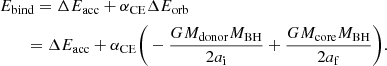\end{matrix}$ $\begin{aligned}&E_{\rm bind} = \Delta E_{\rm acc} + \alpha _{\rm CE} \Delta E_{\rm orb}\nonumber \\&\qquad = \Delta E_{\rm acc} + \alpha _{\rm CE} \Bigg ( -\frac{G M_{\rm donor} M_{\rm BH}}{2 a_{\rm i}} + \frac{G M_{\rm core} M_{\rm BH}}{2 a_{\rm f}} \Bigg ) .\end{aligned}$ (1)

Here, M_donor is the mass of the giant donor that initiates the CE phase, M_core is the mass of its core that becomes the remnant after a successful envelope ejection, M_BH is the mass of the BH accretor, and a_i and a_f is the separation at the onset and at the end of the CE phase, respectively. The α_CE parameter accounts for the fact that not all the orbital energy can be deposited into the envelope without any losses and as such takes a value of between 0 and 1. Notably, α_CE = 1.0 is quite extreme as it assumes no energy loss in any form from the system. For comparison, in their 3D hydrodynamic simulations of the dynamical phase of CE evolution from low-mass giants (typically spanning several years), Nandez et al. (2015), Nandez & Ivanova (2016) found that usually about 30%−40% of the orbital energy leaves the system as residual (mainly kinetic) energy of the unbound ejecta. In 1D synthetic models of the potentially longer lasting (10−1000 years) self-regulated phase, during which most of the input heat is radiated away, Clayton et al. (2017) found α_CE values in the range 0.046−0.25. At the same time, α_CE ≈ 2 was inferred from 1D simulations by Fragos et al. (2019) in the case of NS accretors and α_CE as large as 5 (or even larger) is often used in population synthesis, especially that of compact binary mergers (e.g., Mapelli & Giacobbo 2018). In Sect. 4.1 we further discuss the uncertainties on the value of α_CE together with possibilites of α_CE > 1 considered in the literature.

Following Voss & Tauris (2003) and Kruckow et al. (2016), we estimate the energy feedback from accretion as the Eddington luminosity of the BH (L_Edd) multiplied by the CE duration τ_CE:

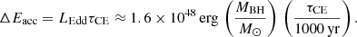$\begin{matrix} Δ E_{acc} = L_{Edd} τ_{CE} \approx 1.6 \times 10^{48} erg (\frac{M_{BH}}{M_{⊙}}) (\frac{τ_{CE}}{1000 yr}) . \end{matrix}$ $\begin{aligned} \Delta E_{\rm acc} = {L}_{\rm Edd} \tau _{\rm CE} \approx 1.6 \times 10^{48}\, \mathrm{erg} \, \left(\frac{M_{\rm BH}}{M_{\odot }}\right) \, \left(\frac{\tau _{\rm CE}}{1000 \,\mathrm{yr}}\right) .\end{aligned}$ (2)

We discuss this approach in view of hydrodynamic models of accretion during CE in Sect. 4.1.

To compute the energy needed to unbind the envelope E_bind we take three terms into account: the energy needed to overcome the gravitational potential of the envelope −E_grav, lowered by the thermal energy stored in the envelope U_th (kinetic energy of particles and the energy stored in radiation, Han et al. 1994) as well as the recombination energy E_rec available if all the ions recombine into atoms and atoms associate into molecules (the latter is mostly relevant for H₂, Ivanova et al. 2015). Therefore, E_bind is calculated as:

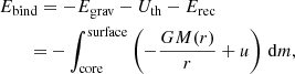$\begin{matrix} E_{bind} = - E_{grav} - U_{th} - E_{rec} \\ = - \int_{core}^{surface} (- \frac{G M (r)}{r} + u) d m, \end{matrix}$ $\begin{aligned}&E_{\rm bind} = -E_{\rm grav} - U_{\rm th} - E_{\rm rec} \nonumber \\&\qquad = - \int _{\rm core}^\mathrm{surface} \left( - \frac{G M(r)}{r} + u \right) \,\mathrm{d}m ,\end{aligned}$ (3)

where u is the internal energy (both thermal and recombination energy) per unit mass. In MESA the value of u in each layer is taken from the tabulated equation of state (Sect. 4.2 of Paxton et al. 2011). We note that it might be more physically accurate to treat the energy from recombination as a separate energy source rather than to include it in the envelope binding energy because this energy is not available immediately, and its release must be triggered at a later stage of the CE phase (Ivanova et al. 2015). It is also not clear how much of this energy can in practice be used to help eject the envelope (Nandez et al. 2015). However, similarly to Wang et al. (2016), we opt to include E_rec in E_bind so that the binding energy computed this way combines all the terms derived from the structure of the giant donor. We note that the contribution of the recombination energy to the total internal energy of massive giant envelopes is relatively small (< 10%, see Kruckow et al. 2016).

An important choice that has to be made when computing E_bind is that of the boundary between the core (which will become the remnant of the giant donor) and the ejected envelope, the so called bifurcation point. Tauris & Dewi (2001) showed that because most of the binding energy is located in deep envelope layers close to the helium core, the exact choice of the bifurcation point can have a substantial impact on the calculated binding energy. A number of criteria for the core-envelope boundary during the CE ejection have been proposed in the literature (see Sect. 4 of Ivanova et al. 2013a). In particular, Ivanova (2011b) suggested that the bifurcation point location can be associated with the point of maximum compression M_cp within the H-burning shell, which is where the value of P/ρ has a local maximum. They argued that for masses M > M_cp the remnant would re-expand on a thermal timescale after the CE ejection or possibly still during the CE phase itself, either causing another phase of mass transfer or prolonging the CE evolution, ultimately leaving behind a remnant with M ≈ M_cp⁵. Kruckow et al. (2016) found that in most giants the location of the maximum-compression point can be approximated by the mass coordinate where X_H = 0.1 and used that as their criterion for the bifurcation point. Here we follow this latter approach; see Sect. 4.6 for further discussion on this topic.

Having computed E_bind from stellar models and assumed the value for α_CE, we can use Eq. (1) to calculate the post-CE separation a_f of a binary with a given BH mass. A successful CE ejection takes place if the remnant core of the giant donor is smaller than its Roche lobe in the post-CE binary. We estimate the size of the remnant R_remnant to be equal to the outer radial coordinate of the core in the pre-CE model of the giant donor multiplied by a factor of two, as guided by Ivanova (2011b), to account for the fact that the compressed core expands in radius during the CE phase itself.

Finally, for practical purposes, the envelope binding energy is often written as (de Kool 1990)

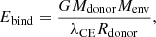$\begin{matrix} E_{bind} = \frac{G M_{donor} M_{env}}{λ_{CE} R_{donor}}, \end{matrix}$ $\begin{aligned} E_{\rm bind} = \frac{G M_{\rm donor} M_{\rm env}}{\lambda _{\rm CE} R_{\rm donor}} ,\end{aligned}$ (4)

where R_donor is the radius of the giant donor, M_env is the mass of its envelope (M_env = M_donor − M_core), and λ_CE is a parameter that depends on the detailed envelope structure. In Appendix A we provide fits to λ_CE values computed in this work, with application to population synthesis.

2.4. Model summary: the “optimistic” choice of assumptions

Our goal is to find the extend to which BH binaries with massive stellar companions can evolve through and survive a CE phase. Therefore, whenever possible, we make choices of assumptions that would facilitate an easier CE ejection. For clarity, these choices are summarized below (see Sects. 2.2 and 2.3 for details). We refer to Sect. 4.1 for a discussion of different assumptions and other caveats of the method.

– For a binary with a giant donor of a given mass and a BH accretor that undergoes a CE evolution, the final separation will be larger (and therefore the CE survival more likely) for larger BH masses, as can be deduced from Eq. (1). Therefore, we assume optimistically low values for the critical (minimum) mass ratios q_crit = M_donor/M_BH that are required for the CE evolution to occur: q_crit; conv = 1.5 for convective-envelope donors and q_crit; rad = 3.5 for post-MS radiative-envelope donors. Additionally, we classify a giant star as already convective when the outermost 10% of the envelope (in mass) is convective (disregarding the sometimes-present insignificantly small surface radiative layers).

– We compute envelope binding energies E_bind under assumptions that all the internal energy as well as the entire energy released during recombination can be used to help unbind the envelope (Eq. (3)).

– We assume that orbital energy from the binary orbit shrinking within the CE can be transferred to the envelope without any losses, that is, α_CE = 1.0 in Eq. (1).

– We assume that the envelope acceleration is perfectly fine-tuned to reach exactly the local escape velocity, that is, there is no term for residual kinetic energy at infinity in Eq. (1).

– We include energy feedback from accretion ΔE_acc = L_Eddτ_CE and assume a relatively long duration of the CE phase, namely τ_CE = 1000 yr (Ivanova et al. 2013a). For instance, for a 1.4 M_⊙ NS this yields ΔE_acc ≈ 2 × 10⁴⁸ erg, whereas for a 20 M_⊙ BH this yields about ΔE_acc ≈ 3 × 10⁴⁹ erg. The relevance of these values compared to the envelope binding energy can be seen in the following section.

3. Results

3.1. The envelope binding energy: impact of the outer convective layer

In Fig. 1 we plot the envelope binding energy E_bind of massive giants (i.e., the post-MS part of the evolution) of several chosen masses at each of the six studied metallicities. Colors in Fig. 1 indicate what fraction f_conv of the envelope mass is in the outer convective zone, that is, f_conv = M_env; conv/M_env, where M_env; conv is the mass of the outer convective zone and M_env is the envelope mass. In particular, f_conv = 0.0 indicates a giant with a radiative outer envelope. The binding energies were computed from stellar models described in Sect. 2.1 under the assumption that all of the thermal energy as well as the recombination energy can be used to help eject the envelope during a CE phase (see Sect. 2.3 for details).

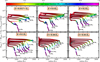Fig. 1.

Envelope binding energies E_bind of massive giants (i.e., the post-MS part of the evolution) as a function of their radius for six different metallicities (selected models from Klencki et al. 2020). See Fig. C.1 for a figure including all the masses in the grid and Fig. C.3 for a figure showing all the corresponding λ_CE values. E_bind combines the gravitational potential energy as well as the internal energy (including the recombination terms); see Eq. (3). Only post-MS evolution is shown. Colors indicate what fraction of the envelope mass is in the outer convective zone (i.e., M_env; conv/M_env). Diamonds (same coloring) and white crosses mark the onset and end of core-helium burning, respectively. Part of the evolution when the radius is increasing beyond the previously largest radius that has been reached, i.e., the part relevant for RLOF and mass transfer, is shaded in black. Development of a deep outer convective envelope layer can lead to a very significant decrease in the binding energy, unless the giant is a HG star (i.e., before the core-helium ignition); see Sect. 3.4 for details.

Diamonds in Fig. 1 mark the onset of core-helium burning (defined as the point when central helium abundance Y_C drops below 0.975), meaning that all of the previous evolution is the Hertzprung-Gap (HG) phase. White crosses correspond to the central helium depletion (Y_C < 10⁻³). At solar metallicity (top-left panel), most of the radial expansion of a giant happens already during the HG phase for all the masses considered here. As the metallicity decreases, more and more massive stars remain relatively compact during their HG evolution and most of the expansion in their case takes place during core-helium burning. Massive models at the lowest metallicity in our grid (Z = 0.01 Z_⊙, the lower right panel) remain compact for even longer and only expand significantly after the central helium depletion. This is a well-known relationship between metallicity and the degree of post-MS expansion of massive giants, details of which are sensitive to a number of poorly constrained ingredients of stellar models such as convective boundary mixing, semiconvection, or rotational mixing (e.g., Georgy et al. 2013; Schootemeijer et al. 2019; Higgins & Vink 2019; Klencki et al. 2020; Kaiser et al. 2020). We note that some of the most massive models in Fig. 1 for metallicities Z ≥ 0.1 Z_⊙ were not evolved all the way until the central helium depletion but only to the point when strong stellar winds started to cause significant shedding of the giant’s envelope, causing it to decrease in radius and begin a blueward evolution in the HR diagram towards the WR stage.

The overall behavior of E_bind as a function of radius in Fig. 1 is similar to what was found in previous studies (Dewi & Tauris 2000; Podsiadlowski et al. 2003; Loveridge et al. 2011; Wang et al. 2016). Notably, some of the models reveal a significant decrease in the envelope binding energy when approaching their largest radii, in some cases by more than an order of magnitude. The sudden drop in E_bind coincides with the point when the outer envelope of the giant becomes convective. This is because the entire outer convective zone of an envelope is located at relatively large radial coordinates and as a result its density is small and is very loosely bound to the star (see Fig. 2 of Podsiadlowski 2001).

However, development of a deep outer convective layer does not always lead to a significant decrease in the binding energy. The most massive giants at metallicities Z = 1.0 Z_⊙, 0.4 Z_⊙, 0.2 Z_⊙, and 0.1 Z_⊙ in Fig. 1 expand enough to become convective (up to f_conv ≈ 0.6), yet their E_bind barely decreases as a result of that. Those are the models in which the outer layers already become convective during the HG phase, that is, before the onset of core-helium burning, as indicated by the diamonds in Fig. 1. As a result, because of its impact on the radial expansion of massive giants, metallicity has an indirect but very strong effect on the binding energy of a convective-envelope giant. The reason why the binding energy does not significantly decrease when the envelope becomes convective in HG giants requires a detailed explanation; see Sect. 3.4.

3.2. Common-envelope ejectability in progenitors of BBH mergers

Here we study the possibility of ejecting envelopes with E_bind computed in the previous section during the CE evolution (i.e., the CE ejectability) in binaries with stellar BH companions, potential progenitors of BBH mergers. Our goal is to find the maximum parameter space in which the CE ejection is feasible according to energy budget considerations introduced in detail in Sect. 2.3. To this end, we make a number of optimistic assumptions summarized in Sect. 2.4, each of them increasing the energy sources relative to energy sinks and thus making a CE ejection more likely.

For each evolutionary track of a massive giant analyzed in this work, we compute what would be the outcome separation of a CE phase initiated by that star at any given point during its post-MS evolution assuming a circular binary in which the companion is a BH with mass M_BH = M_donor/q_crit (we note that M_donor < M_ZAMS due to wind mass loss, where ZAMS stands for zero-age main sequence). Survival of the CE evolution is then determined based on the size of the remnant core of the CE donor R_remnant (estimated as twice the radial coordinate of the outer core boundary in the pre-CE structure of the donor; see Sect. 2.3) compared to the size of its Roche lobe in the post-CE binary R_{RL; post-CE}. Values R_remnant/R_{RL; post-CE} > 1 indicate a merger during the CE phase, whereas R_remnant/R_{RL; post-CE} ≤ 1 indicates a successful CE ejection.

The result is showed in Fig. 2 where, as a function of M_ZAMS and the radius of the giant at the onset of the CE phase, we color-code what would be the resulting ratio R_remnant/R_{RL; post-CE} in a post-CE binary. We note that at solar metallicity (top left panel), stars above 60 M_⊙ do not expand in their post-MS evolution because of strong mass-loss in winds, and this is the reason they do not show in Fig. 2 (this result depends on the assumed mass-loss recipe and could to some extent be affected by the numerical accuracy of MS models with inflated envelopes; see Appendix B). Missing masses (one at Z = 0.04 Z_⊙ and two at Z = 0.01 Z_⊙) are nonconverging MESA models.

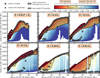Fig. 2.

Common-envelope ejectability in binaries with massive giant donor stars and BH companions. For each evolutionary track of a massive giant with M_ZAMS between 10 and 80 M_⊙, we compute what would be the outcome of a CE phase initiated by that star at any given point during its post-MS evolution in a circular binary with a BH companion with mass M_BH = M_donor/q_crit (see text for detailed assumptions). The resulting ratio of the size of the remnant core of the CE donor R_remnant and the size of its Roche lobe R_{RL; post-CE} is color-coded in the figure as a function of M_ZAMS and the radius of the giant at the onset of the CE phase. Radii above the white diamonds (crosses) indicate giants that are past the onset (end) of core-helium burning in their evolution. The hatched region marks the parameter space where the giant donor has an outer convective envelope with f_conv = M_conv/M_env ≥ 0.1. The dotted region marks the parameter space where the CE ejection is possible (i.e., R_remnant/R_{RL; post-CE} < 1.0).

The most striking finding is that the parameter space for successful CE ejections (marked as the dotted area) is almost exclusively limited to cases in which the CE evolution is initiated by a giant donor with an outer convective envelope (marked by the hatched area). The only exception are some of the radiative-envelope donors with M_ZAMS ≲ 40 M_⊙ at Z = 0.04 Z_⊙ and M_ZAMS ≲ 60 M_⊙ at Z = 0.01 Z_⊙. This is the result of convective-envelope giants having smaller envelope binding energies compared to radiative-envelope stars (see Fig. 1 and the associated text), combined with the fact that q_crit; conv < q_crit; rad, which means that BH accretors can be more massive in CE events initiated by convective-envelope donors.

We can also see in Fig. 2 that among the potential CE survivors, the R_remnant/R_{RL; post-CE} ratio is either only slightly smaller than 1.0 (yellow to orange colors) or significantly smaller than 1.0 (dark red colors). Generally, the first group corresponds to convective giants that are still at the HG phase (below diamonds in Fig. 2) and their E_bind did not decrease as significantly with the increasing convective-envelope mass fraction f_conv (even for f_conv ≳ 0.6), as also seen in Fig. 1. Given a number of optimistic assumptions in our model, it is uncertain whether or not models from the first group, with the relatively high binding energies, can survive the CE phase (see also Fig. 5 below). The second group are cases in which the CE evolution is initiated by a much more evolved star, with a helium-depleted core (above the crosses in Fig. 2) and a deep outer-convective envelope f_conv > 0.5. The envelopes of such giants are very loosely bound (see Sect. 3.1) and not much orbital shrinkage is needed to provide energy for their ejection. As a result, the energy budget method predicts R_remnant/R_{RL; post-CE} ratios that are below 0.1. In reality, it seems unlikely that the remnant of the donor would fill such a small fraction of its Roche lobe in the post-CE system because in that case the companion would never be at the bottom layers of the donor’s envelope, and would therefore be unable to help in their ejection. As such, very small R_remnant/R_{RL; post-CE} ratios in Fig. 2 should rather be interpreted as cases in which the CE ejection can be easily achieved in terms of the energy budget, not as a reliable prediction of the post-CE binary separation.

The above distinction between the two types of convective-envelope donors also shows that the evolutionary stage of the donor can have a significant impact on the outcome of the CE phase. We illustrate the differences between envelope structures of giants that become convective during the rapid HG expansion and those that reach the convective-envelope stage later during their evolution in Sect. 3.4. Notably, whether a star becomes convective during the HG expansion or only later during its evolution is an uncertain outcome of detailed stellar models but its relation to metallicity appears robust (e.g., Schootemeijer et al. 2019; Klencki et al. 2020).

Even though BH binaries are the main focus of this study, we also consider CE ejectability in systems in which the accretor is a NS with M_NS = 2 M_⊙ (with all the other assumptions being the same). The result is plotted in Fig. C.2. Because of the lower accretor mass, the parameter space for CE ejection in NS binaries is smaller than in the case of BH binaries. Interestingly, it is limited to cases in which the donor is already a core-helium depleted star. In such systems there might be no additional case BB mass transfer phase after a successful CE ejection, in contrast to what has been advocated in the classical picture of the double NS binary formation (for a recent review see Tauris et al. 2017). We leave further discussion of this finding to future studies.

In Fig. 3, similar to Fig. 6 of Kruckow et al. (2016), we explore how several variations in the assumptions of the default model would affect the separation of the post-CE binary a_post-CE and the CE ejectability. We examine the case of a giant CE donor with M_ZAMS = 55 M_⊙ at Z = 0.2 Z_⊙ metallicity, showing a_{post − CE} as a function of its radius at the moment of Roche-lobe overflow (RLOF). The default “optimistic” model is plotted in blue as model (a); see Sect. 2.4 for the summary of its assumptions. Cases where a_post-CE is greater than the minimum separation required to avoid a merger (marked as a black dashed line) is the parameter space for CE ejectability. We note that this is limited to convective-envelope donor cases (f_conv > 0.1). Slow changes in the dashed line are related to the evolution of the core radius (contraction) as well as to a transition from the radiative to the convective envelope stage at around R_donor ≈ 1700 R_⊙, at which point the assumed binary mass ratio decreases from q_crit; rad = 3.5 to q_crit; conv = 1.5.

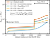Fig. 3.

Exploring CE ejectability for a BH binary with a M = 55 M_⊙ giant donor at Z = 0.2 Z_⊙ metallicity as a function of the giant’s radius at the onset of a CE phase. See text for the explanation of different models (a)–(e). Cases where the post-CE separation a_post-CE is greater than the minimum separation required to avoid a merger (marked as a black dashed line for models (a)–(d) and a dashed purple line for model (e)) survive the CE phase.

Model (b), plotted in green in Fig. 3, is different from the default model in that it does not include the ΔE_acc term in Eq. (1). It corresponds to a situation where the energetic feedback from accretion is significantly smaller than the Eddington luminosity or where the duration of the CE phase is much shorter than the assumed 1000 yr. Excluding E_acc from the energy budget affects the post-CE separation by less than a factor of two for the 55 M_⊙ donor in Fig. 3. The effect is larger for lower mass stars (see for example a 30 M_⊙ donor case in Fig. 4) because of their lower binding energies. We note that ΔE_acc ∝ M_accretor (Eq. (2)), and so for a given mass ratio M_donor/M_accretor = q_crit the energy from accretion scales linearly with the donor mass. We discuss super-Eddington accretion during a CE phase in Sect. 4.1.

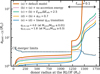Fig. 4.

Same as Fig. 3 but for a 30 M_⊙ model at 0.2 Z_⊙ metallicity. For the donor radii R ≳ 1400 R_⊙ the outer envelope becomes deeply convective during a core-helium burning stage, which causes a significant decrease in the binding energy of the model (Fig. 1) and an increase in the post-CE separation a_post-CE.

Instead of relating the change in orbital energy ΔE_orb to the envelope binding energy E_bind via the α_CE parameter, one can relate ΔE_orb to just the gravitational potential component of the binding energy: ΔE_grav/ΔE_orb = α_grav. In 1D hydrodynamic simulations of an inwardly spiralling CE inside the envelope of a 12 M_⊙ red supergiant, Fragos et al. (2019) find α_grav ≈ 2.7. Three-dimensional models of the CE phase from low-mass giants by Passy et al. (2012) and Ohlmann et al. (2016) find similar values of α_grav ≈ 2.0 and ≈2.5, respectively. Model (c) in Fig. 3 (in red) assumes α_grav = 2.5 and is in fact very similar to the same model but with α_CE = 1.0 (in green). This can be expected based on the typical ratio of thermal internal energy U_th and the gravitational potential energy E_grav in a giant’s envelope; see Sect. 3.2 in Fragos et al. (2019).

Importantly, the assumption of α_CE = 1.0 does not only imply perfect energy transfer (e.g., no radiative losses), but also perfect fine-tuning when the ejected envelope becomes accelerated to gain precisely the local escape velocity. In reality, this is unlikely to be the case. Nandez et al. (2015), Nandez & Ivanova (2016) carried out 3D hydrodynamic simulations of CE events with low-mass giants and found that typically about 30%−40% of the orbital energy leaves the system as residual (mainly kinetic) energy of the unbound ejecta. This corresponds to model (d) in Fig. 3, with α_CE = 0.7. We note that in this model, only half of the convective-envelope donor cases survive the inward spiralling of the CE (the orange line rises above the black dashed threshold in the middle of the f_conv > 0.1 region).

Finally, in model (e) plotted in purple we also apply a smooth transition of the critical mass ratio from q_crit = 4.0 for radiative donors with M_conv/M_star ≤ 0.01 up to q_crit = 1.8 for convective-envelope giants with M_conv/M_star ≥ 0.3 as a linear function of M_conv/M_star. This makes this model consistent with the results of Pavlovskii & Ivanova (2015), who find q_crit; conv between 1.5 and 2.2 for giants with deep convective envelopes of M_conv/M_star ≥ 0.3 and q_crit > 3.5 for less convective giants. Our default classification criteria for convective-envelope donors (f_conv = M_conv/M_env ≥ 0.1) also includes the in-between cases of mostly radiative-envelope donors with relatively shallow convective envelopes, for which the mass transfer is more stable than for giants with deep convective envelopes. The CE ejection in model (e) is only possible in a small number of cases when the 55 M_⊙ giant is close to its maximum size and its outer convective envelope is the most extended.

In Fig. 4 we plot the same model variations as in Fig. 3 but for a lower mass, namely 30 M_⊙, giant (also at Z = 0.2 Z_⊙ metallicity). The main difference is that for donor radii above ∼1450 R_⊙ all explored variations result in a successful CE ejection. This is because at that point the 30 M_⊙ model develops a deeply convective envelope at late stages of core-helium burning, which leads to a significant decrease in its binding energy for R ≳ 1400 R_⊙ (see Fig. 1). In fact, at those stages the envelope is so loosely bound that the accretion term ΔE_acc alone is larger than E_bind. Figure 4 illustrates that in models with loosely bound deep convective envelopes the estimated post-CE separation is often significantly larger than the CE-merger limit. In those cases (appearing in dark red in Fig. 2) the CE ejectability does not significantly depend on the particular choice of assumptions for the energy budget.

Models (b)-(e) in Fig. 3 show that our reference model (a) yields a reasonable but very optimistic result in terms of CE ejectability shown in Fig. 2. For comparison, in Fig. 5 we make less optimistic but probably more realistic assumptions of α_CE = 0.7 and a smooth linear transition of q_crit between radiative and convective envelope donors as in model (e) above. The result is a significantly reduced parameter space for CE survival, mostly limited to the cases of loosely bound convective envelopes in core-helium burning or more evolved giants.

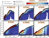Fig. 5.

Same as Fig. 2 but assuming a more realistic energy budget and the mass transfer stability criteria: α_CE = 0.7 instead of α_CE = 1.0 and a smooth transition of q_crit from q_crit = 4.0 for radiative donors with M_conv/M_star ≤ 0.01 up to q_crit = 1.8 for convective-envelope giants with M_conv/M_star ≥ 0.3 as a linear function of M_conv/M_star. We note that f_conv = M_conv/M_env, and f_conv > 0.1 region is hatched in the figure.

3.3. It has to be cool: tight link between the CE donors and red supergiants

In the previous section we show that unstable mass transfer evolution followed by a CE phase and a successful CE ejection in binaries with BH or NS accretors is only energetically feasible (even under optimistic assumptions) if the donor star is a massive supergiant with an outer convective envelope; see Figs. 2 and C.2. Observationally, such stars appear as red supergiants (RGSs) with effective temperatures of about log(T_eff/K) ≲ 3.7 (depending on the exact position of the Hayashi line at a given metallicity).

We illustrate this in an HR diagram for the SMC-like metallicity (Z ≈ 0.2 Z_⊙Venn 1999) in Fig. 6, in which the estimated region of CE ejectability is marked in green (this corresponds to the dotted area in the top-right panel of Fig. 2). The part of that parameter space marked in violet are cases in which the CE ejection is also possible with NS accretors.

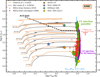Fig. 6.

HR diagram for the SMC-like metallicity (Z ≈ 0.2 Z_⊙Venn 1999) in which the green area marks the position of donor stars at the onset of RLOF for which a CE evolution with a successful CE ejection in BH binaries is possible. A smaller violet area marks the subset of donors for which CE ejection is also possible in the case of NS accretors (M_NS = 2 M_⊙). A definitive association of donors to successful CE evolution events with cool (red) supergiants ( log(T_eff/K) ≲ 3.7) is clear. Two sets of selected stellar tracks are plotted: models from Klencki et al. (2020), which are the main focus of this paper, and models from Georgy et al. (2013) computed with the GENEVA code. Physical parameters of RSGs observed in the SMC are taken from Levesque et al. (2006) and Davies et al. (2018). The black dashed line marks the empirical Humphreys-Davidson (H-D) limit, beyond which almost no stars in the Milky Way or in the LMC are observed (Humphreys & Davidson 1979, 1994; Ulmer & Fitzpatrick 1998). The light-blue line shows the threshold effective temperature below which at least 10% of the mass of models from Klencki et al. (2020) is in the outer-convective envelope. Colored stars mark the inferred physical parameters of three different massive star progenitors of luminous-red novae (LRNe; Smith et al. 2016; Blagorodnova et al. 2017; Mauerhan et al. 2018). The yellow diamond shows the RSG donor in a pulsating ultra-luminous X-ray (ULX) source NGC 300 ULX-1 (Heida et al. 2019a).

For comparison, we mark the positions of known RSGs in the SMC from the samples of Davies et al. (2018, with effective temperatures based on spectral-energy density fits) and Levesque et al. (2006, with effective temperatures from atmospheric model fits).

For reference, the light-blue line around log(T_eff/K) ≈ 3.65 marks the threshold temperature T_eff; th below which at least 10% of the mass of the star is in the outer-convective envelope (from Sect. 3.4 of Klencki et al. 2020). The fact that many of the RSGs in the sample collected by Davies et al. (2018) are hotter than T_eff; th and fall outside of the predicted temperature range of RSGs in the green area in Fig. 6 is a likely indication that the value of the mixing-length parameter α_ML = 1.5 in the models from Klencki et al. (2020) is somewhat too small⁶.

The brightest RSG in the SMC has a luminosity of log(L/L_⊙) = 5.55 ± 0.1 (Davies et al. 2018). A similar empirical upper luminosity limit for RSGs of log(L/L_⊙)_RSG; max ≈ 5.6 − 5.8 has been found also for other local galaxies of different types and compositions: the Milky Way (Z = 0.02, Levesque et al. 2006), M31 (Z = 0.04, Neugent et al. 2020), the Large Magellanic Cloud (Z = 0.007, Davies et al. 2018), and several dwarf irregular galaxies ([Fe/H] between −1.0 and −0.4, Britavskiy et al. 2019). This limit is marked in Fig. 6 at an approximate luminosity log(L/L_⊙)_RSG; max = 5.7, which corresponds to stars with initial masses M_ZAMS ≈ 40 M_⊙. The existence of the empirical upper luminosity limit log(L/L_⊙)_RSG; max could be an indication that more massive stars never expand to reach the RSG stage during their evolution, because of for example extensive mass loss at the uncertain luminous blue variable stage. In view of our findings, this would likely prevent donors with M_ZAMS ≳ 40 M_⊙ from forming BBH mergers in the CE evolution channel.

Lack of RSGs above a certain luminosity limit has been purposefully recovered in various stellar tracks of massive stars. As an example, in Fig. 6 we plot several rotating stellar tracks computed with the GENEVA code for Z = 0.002 (Georgy et al. 2013). For reference, we also show a few corresponding tracks from Klencki et al. (2020) that were used to compute envelope binding energies in this work⁷. The lack of most luminous RSGs in the GENEVA tracks is most likely a result of increasing mass-loss rates in stars with super-Eddington layers (Ekström et al. 2012) as well as of suppressing density inversions in radiation-dominated stars by using a mixing length taken on the density rather than on the pressure scale height (Appendix A of Klencki et al. 2020). We discuss the empirical log(L/L_⊙)_RSG; max limit in the context of CE evolution and the formation of BBH mergers in Sect. 4.2.

It is worth noting that CE evolution in a binary with a BH or a NS accretor is preceded by a phase of essentially stable mass transfer that takes place between the moment of RLOF and the onset of the CE phase (MacLeod et al. 2018a,b; MacLeod & Loeb 2020a). During this stage the mass transfer rate gradually increases at a rate which is primarily dictated by the thermal timescale of the envelope of the donor (also in the case of convective-envelope donors; see Woods & Ivanova 2011; Pavlovskii & Ivanova 2015). In the case of massive donors, this indicates a duration of the order of ∼10⁴ yr, and a loss of even ∼30% mass from the envelope of the donor (MacLeod & Loeb 2020b, also Ivanova, priv. comm.)⁸. Observationally, a system at this stage would likely appear as a bright X-ray binary: a ULX. In the case of potential CE survivors among BH and NS binaries, this corresponds to ULXs with RSG donor stars. Several such systems with donor stars spectroscopically confirmed to be RSGs are known to date (Heida et al. 2015, 2016, 2019b; Lau et al. 2019). In the case of one of the sources, a pulsating ULX dubbed NGC 300 ULX-1, Heida et al. (2019b) were able to model the spectrum of the optical counterpart as a sum of three components: a blue excess (likely due to X-ray irradiation), a red excess (likely due to dust), and a stellar atmosphere model of an RSG with T_eff = 3650 - 3900 K and log(L/L_⊙) = 4.25 ± 0.1 (marked in Fig. 6). López et al. (2020) completed a systematic search for near-infrared candidate counterparts to nearby ULXs and concluded that ULXs with RSG donors constitute about ∼4% of the observed ULX population, which is about four times more than predicted by population-synthesis models (Wiktorowicz et al. 2017). One reason for this discrepancy could be that rapid binary evolution codes assume that the moment of RLOF is also the onset of CE evolution, without modelling the intermediate mass transfer phase.

One observational signature of the CE phase itself are LRNe, red transients characterized by a rapid rise in luminosity followed by a lengthy plateau (Soker & Tylenda 2003; Kulkarni et al. 2007; Tylenda et al. 2011; Ivanova et al. 2013b; Kochanek et al. 2014; Howitt et al. 2020). In several cases, archival multiband observations from before the LRN have revealed the progenitors to be consistent with massive giants: notably a ∼18 M_⊙ progenitor to M101-OT (Blagorodnova et al. 2017) and a ∼60 M_⊙ progenitor to SNHunt 248 (Mauerhan et al. 2018), as well as a putative single-band detection of an LBV-like progenitor to NGC 4490-OT (Smith et al. 2016). In none of these cases was the progenitor consistent with a RSG; see Fig. 6. According to our findings, this might be an indication that these CE events finished in mergers, although our results may not be directly applicable to CE cases with stellar accretors. As a final remark, it was recently shown by Ginat et al. (2020) that inward spiralling of compact accretors during the final stages of CE evolution could produce a GW signature which might be detectable by the next-generation GW detectors such as Laser Interferometer Space Antenna (LISA).

3.4. A detailed look at the structure and the binding energy of convective-envelope giants

In Sect. 3.1 we found that the envelope of a massive giant can become significantly less bound when it transitions from a radiative to a convective state, with E_bind decreasing by an order of magnitude or more. An exception to this rule are giants that become convective already during the HG phase, for which the decrease in the binding energy is much less significant. In this section we explain the origin of this behavior.

In Fig. 7 we illustrate this transition for a model with M_ZAMS = 47.5 M_⊙ and Z = 0.1 Z_⊙, which develops a deep outer convective envelope during late stages of core-helium burning and is an example of a model for which the associated decrease in E_bind is very significant. Panel 7a shows the Kippenhahn diagram of the model (excluding the initial part of the MS when X_H; C > 0.55) with stellar radius plotted in red. In panel 7b, one can see that the binding energy E_bind slowly decreases during the core-helium burning phase and then decreases significantly as the envelope becomes deeply convective (and f_conv increases).

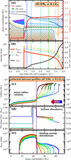Fig. 7.

Detailed look at the evolution of a M_ZAMS = 47.5 M_⊙ model at Z = 0.1 Z_⊙ metallicity. Panel a shows the Kippenhahn diagram with stellar radius over-plotted in red. We note that the purple color shows regions of semiconvective mixing. Panel b shows the time evolution of the binding energy E_bind and its components: E_grav and E_int = U_th + E_rec (see Eq. (3)) together with the convective envelope mass fraction f_conv. Panels c–e show several internal profiles of the model, the position of which are marked in panels a and b with dashed vertical lines in corresponding colors. The outer convective zone is marked in bold in panel c. Solid vertical lines in panels c–e mark the core-envelope boundary for the CE evolution (i.e., the bifurcation point at X_H = 0.1).

The next three panels of Fig. 7 show a more detailed view of the internal structure of the star at several selected moments during its evolution. Panel 7c shows the internal mass-radius profiles, with the outer convective zone being marked in thicker lines. The bifurcation point of each profile, which is the point that divides between the ejected envelope and the remaining remnant of the donor in a CE event, is marked with a solid vertical line located at X_H = 0.1. With time (i.e., profile colors changing from blue to red) the inner part of the star contracts as a result of continuous burning in the core. On the other hand, as the envelope becomes increasingly convective, the outer layers in the star move to larger radial coordinates. The point in between the contracting and the expanding layers of the star, located at the mass coordinate of about ∼23 M_⊙ in panel 7c, is an important divergence point. The helium abundance profiles in panel 7d reveal that the divergence point coincides with a steep composition jump at the boundary between the helium core (where X_He ≈ 1 in the helium shell) and the H-rich envelope. Importantly, it also closely coincides with the assumed location of the bifurcation point, marked with dashed vertical lines. In other words, the part of the giant above the bifurcation point, which would need to be ejected in a successful CE phase, is also the part that expands to larger radii coordinates as the outer envelope becomes increasingly convective. As a result, the entire envelope becomes less gravitationally bound (see panel 7e) and E_bind steeply decreases when f_conv increases.

As pointed out above, giants that expand to develop a deep outer convective envelope already during the HG phase do not see their envelope binding energies decrease in a significant way as a result of that. In Fig. 8 we illustrate an example of such a case, a model with M_ZAMS = 47.5 M_⊙ and Z = 0.4 Z_⊙; in panels (a)-(e) we plot the same quantities as in the corresponding panels in Fig. 7. We note that the two upper panels, 8a and 8b, have a different scaling on the x-axis (linear) than panels 7a and 7b (logarithmic) as they only focus on the part of the evolution during which the radius substantially increases (the part relevant for mass transfer interactions). The decrease in E_bind at around 4.54 Myr in panel 8b is initiated by a contraction of the inner parts of the star after the end of MS and the associated expansion of the outer layers (before the outer envelope becomes convective), as also seen at the very beginning of E_bind evolution in panel 7b for the Z = 0.1 Z_⊙ giant. During the development of an outer convective envelope (f_conv ≈ 0.6) the binding energy decreases by less than a factor of two.

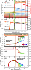Fig. 8.

Similar to Fig. 7 but for a model with M_ZAMS = 47.5 M_⊙ at Z = 0.4 Z_⊙ metallicity. The two upper panels a and b are centered on the evolutionary phase during which the radius substantially increases, which is mainly the phase of rapid HG expansion. The different structural response of the envelope to the outer convective zone in panel c, associated with differences in the abundance profile in panel d, leads to a much smaller impact of the increasing f_conv on the envelope binding energy E_bind (see text for details).

The bottom three panels in Fig. 8 illustrate the essential difference in the structure of a convective HG star compared to a more evolved convective giant from Fig. 7. As the outer convective zone extends deeper and deeper inside the envelope (panel 8c), the outer layers of the star expand to larger radial coordinates, while the inner part of the star slightly contracts. This is a similar behavior to that seen in panel 7c. However, in the case of the HG giant in panel 8c, the divergence point between the contracting and the expanding part of the star is no longer located very close to the helium-core boundary at a mass coordinate ≈23 M_⊙ (where X_He ≈ 1) but appears higher up inside the star at ≈26 M_⊙. We find that such a different location of the divergence point in HG giants is associated with a distinctively different internal abundance profile; see panel 8d. In regards to the composition jump near the helium core where X_He ≈ 1 is smaller than that in panel 7d, the helium abundance only drops down to X_He ≈ 0.75, forms a plateau, and then starts to gradually decrease again at a mass coordinate of about 26 M_⊙. One can see that the divergence point is roughly associated with the secondary drop when X_He decreases below ∼0.75. The consequences of the structural change on the binding energy distribution within the envelope can be seen in panel 8e. The ∼2 − 3 M_⊙ of helium-dominated material (X_He ≈ 0.75) at the bottom of the envelope move slightly inward inside the star and their binding energy increases, which counteracts the decreasing binding energy of the outer convective layers. As a result, the overall binding energy of the envelope remains roughly unaffected.

We find that the example in Fig. 8 is representative for models of giants that reach the convective-envelope stage during HG expansion. The reason for the crucial difference in helium abundance profiles between panels 7d and 8d has to do with the size of an intermediate convective zone (ICZ)⁹ that develops in a star on top of the hydrogen-burning shell right after the end of the MS, that is, during the phase of rapid HG expansion when the star is out of thermal equilibrium (e.g., Langer et al. 1985; Schootemeijer et al. 2019; Kaiser et al. 2020).

In models that by this stage have already expanded all the way to the red-giant branch and developed an outer convective envelope, the ICZ tends to quickly disappear, as in the model in Fig. 8 and as also found by previous authors (e.g., Langer et al. 1985; Schootemeijer et al. 2019; Davies & Dessart 2019; Kaiser et al. 2020). In contrast, in models where the star expands less during the HG stage and stably burns helium as a blue or yellow supergiant, the ICZ does not disappear quite as quickly and becomes more extended (in mass coordinate), as in the model in Fig. 7. A more extended ICZ means that more hydrogen is mixed from the H-rich envelope into the He-rich layers above the helium core, and as a result the composition jump at the core-envelope boundary is larger and the helium abundance at the bottom of the envelope is smaller, as can be seen by comparing Fig. 7d with Fig. 8d. Another difference between the models in Figs. 7 and 8 is that in the 0.1 Z_⊙ case the H-burning shell remains convective throughout the core-helium burning while in the 0.4 Z_⊙ case the ICZ disappears and the H-burning shell becomes radiative. Compared to the role played by the ICZ, which is present in both cases, the nature of the H-burning shell does not appear to be an important factor for the abundance profiles shown in Figs. 7d and 8d; these abundance patters are already determined by the ICZ.

The reasoning presented above explains the relation between the degree of expansion during the HG phase, the size of the ICZ, and the abundance profile of deep envelope layers. However, the precise extent of the ICZ in a given model has to be considered as highly uncertain; it is sensitive to the assumed efficiency of semiconvective mixing (Schootemeijer et al. 2019), convective overshooting (Kaiser et al. 2020), numerical accuracy of stellar models (see Appendix B and Farmer et al. 2016), and treatment of convective boundaries in regions with steep composition changes (see e.g., the convective premixing scheme introduced in MESA, Paxton et al. 2019). However, perhaps most importantly, the extent of the ICZ likely depends on the abundance profile above the H-burning shell left behind by the previous evolution. It is therefore sensitive to rotational mixing (Georgy et al. 2013) and to (semi)convective mixing above the H-burning core already during the MS (Farmer et al. 2016). Additionally, in the case of a past accretor from previous mass transfer phases (which is most definitely relevant for the case of companions in BH binaries studied here), the abundance profile above the H-burning shell can be significantly different compared to an unperturbed single stellar model due to rejuvenation and growth of the H-burning core of the mass gainer (Hellings 1983, 1984; Braun & Langer 1995; Wellstein et al. 2001; Dray & Tout 2007).

It is also worth mentioning that the relation between the degree of HG expansion and the degree of mixing in the ICZ operates both ways: if the mixing is not very efficient, then a certain model may expand to the RSG stage, whereas the same model but with efficient mixing (e.g., by semiconvection or rotationally induced mixing) will in some cases expand much less and burn helium as a blue supergiant (see Appendix B of Klencki et al. 2020). This provides a possibility to calibrate models using the observed ratio of blue to red supergiants. For example, the post-MS expansion of the models used in this study was calibrated to match the ratio observed in the SMC.

In summary, the internal structure and chemical profiles presented here suffer from uncertainties in various internal mixing processes and numerical challenges associated with the ICZ, and are likely affected by a previous accretion phase. Nevertheless, it seems reasonable to expect some systematic differences in the envelope structure (and the binding energy) between stars that become convective during the HG phase and those that only become convective much later during there evolution. The examples shown in Figs. 7 and 8 offer some guidance as to what these differences could look like.

It is interesting to speculate about the consequences of different envelope structures of giants seen in Figs. 7 and 8 for the CE evolution itself, in particular given that the location of the divergence point in the Z = 0.4 Z_⊙ model is substantially different from that of the bifurcation point (under usual assumptions). We discuss this further in Sect. 4.6. The examples given in Figs. 7 and 8 show that the internal envelope structure of a convective-envelope supergiant can depend significantly on the evolutionary stage of the star.

4. Discussion

4.1. How robust is the prediction that CE evolution in BH binaries requires RSG donors?

In Sect. 3.2 we show that the parameter space for CE ejectability in binaries with BH or NS accretors is limited to donors with outer convective envelopes, that is, cool supergiants (RSGs, see Fig. 6). This conclusion was reached by pursuing a very optimistic case of the energy budget of CE evolution (Sect. 2.4). In particular, we assumed that the entire energy input from orbital shrinkage, the internal energy of the envelope, recombination energy, and the energy input from accretion can be transferred into kinetic energy and used to help unbind the envelope. We also assumed no energy loss in any form (i.e., α_CE = 1.0), neglecting energy sinks such as radiation from the surface or excess kinetic energy in outflows. These assumptions are clearly extreme. For instance, in view of hydrodynamic simulations, a more realistic assumption would be α_CE ≲ 0.7 or even α_CE ∼ 0.1 during the possibly reached self-regulated phase of the CE evolution (see Sect. 2.3 for details). These results suggest that the parameter space for a successful CE ejection in Figs. 2 and 6 is most likely an upper limit on the true (realistic) CE ejectability; see for example Fig. 5.

From the observational side, various attempts have been made in the past to constrain the CE ejection efficiency α_CE by linking post-CE systems to their reconstructed pre-CE progenitors (e.g., Nelemans et al. 2000; Zorotovic et al. 2010, 2011; De Marco et al. 2011; Davis et al. 2012; Portegies Zwart 2013). While most of these results suffer from uncertainties in the reconstruction technique of pre-CE parameters and the α_CE values they yield are degenerated with the binding energy parameter λ_CE, for the majority of the post-CE systems the inferred values of α_CE are clearly below 1.0, although in some cases only when the internal envelope energy is included (see e.g., De Marco et al. 2011, for a discussion of the impact of thermal energy on the inferred α_CE values). However, it is worth pointing out that the formation of three double helium white dwarfs analyzed by Nelemans et al. (2000) as well as one of the post-CE systems analyzed by De Marco et al. (2011) seemingly cannot be reconstructed without α_CE > 1. This might be a signal of the limitations of the energy budget formalism, some of which we discuss below. This might also be an indication that CE evolution does not always take place when we expect it to. Another type of system for which values of α_CE > 1.0 were advocated, and perhaps more relevant in the context of massive stars and BBH merger progenitors, are BH low-mass X-ray binaries (BH-LMXBs, e.g., Kalogera 1999; Podsiadlowski et al. 2003). In Sect. 4.5 we analyze their case in more detail and argue that α_CE ≤ 1.0 could potentially be sufficient.

There are two caveats of our method: the possible contribution of other energy sources in CE ejection (unaccounted for in our energy budget) and lower envelope binding energies. Apart from the energy terms considered in this work, other energy sources have been discussed in the literature. One possible addition is the energy from nuclear burning (e.g., Ivanova & Podsiadlowski 2003). However, as pointed out by Ivanova et al. (2013a), when the donor’s envelope is lifted from the core, the nuclear energy input is most likely going to decrease with respect to radiative losses from an expanding emitting area¹⁰.

Another addition to the energy budget that has been proposed is an enthalpy term P/ρ (Ivanova & Chaichenets 2011). While enthalpy is primarily responsible for energy redistribution (rather than being a new energy source Ivanova et al. 2013a), it leads to solutions with quasi-steady outflows from envelopes even before their total energy becomes positive. However, this requires the CE ejection to happen on a long thermal timescale (e.g., after a self-regulated spiral-in phase), at which point radiative losses increase significantly and our assumptions with α_CE = 1.0 are extremely optimistic (e.g., Clayton et al. 2017 find α_CE between 0.046 and 0.25).

Here, we considered energy input from accretion ΔE_acc estimated as Eddington luminosity of the compact accretor multiplied by 1000 yr, similarly to Voss & Tauris (2003) and Kruckow et al. (2016). It should be noted that the accretion rate does not need to be Eddington limited due to neutrino cooling and photon trapping inside the accretion flow inside the CE (e.g., Houck & Chevalier 1991; Edgar 2004; MacLeod & Ramirez-Ruiz 2015a). Furthermore, in rare instances super-Eddington accretion during a CE phase could produce BHs with masses in the PISN mass gap (van Son et al. 2020). While the luminosity that is radiated away and absorbed by the surrounding envelope is still likely of the order of the Eddington luminosity, the total accretion luminosity estimated as η Ṁc² (with η ∼ 0.1) could be in some cases much higher (MacLeod & Ramirez-Ruiz 2015b; MacLeod et al. 2017; De et al. 2020). If the accretion is taking place through an accretion disk then polar outflows or jets could serve as a way of transferring this super-Eddington power to the envelope, thus helping in its ejection (Armitage & Livio 2000; Soker 2015). However, among other uncertainties related to this process, it is unclear whether a persistent accretion disk forms around an embedded compact object. Hydrodynamic simulations by Murguia-Berthier et al. (2017) suggest that accretion through a disk is a rare and transitory phase, which may occur when a BH or a NS passes through zones of partial ionization in the outer envelope layers.

Apart from the uncertainties of the CE energy budget discussed above, there are caveats associated with calculations of envelope binding energies E_bind of massive giant donors. First, the value of E_bind can be very sensitive to the location of the bifurcation point, that is, the lower limit in the integral in Eq. (3). We discuss this further as a partial envelope ejection scenario in Sect. 4.6. Second, we used single stellar models to infer binding energies of stars which have most likely been mass gainers in a mass transfer phase in the past. While this is common practice, the envelope structure of a rejuvenated star could be quite different from that of a single unperturbed star of the same mass (Braun & Langer 1995; Wellstein et al. 2001; Dray & Tout 2007). Third, E_bind values computed from single stellar models represent the binding energy at the point of RLOF rather than at the onset of the CE phase. In reality, before the mass transfer rate increases sufficiently and the system becomes dynamically unstable, a giant donor is likely going to lose a sizable part of its envelope as a result of pre-CE mass transfer (MacLeod & Loeb 2020b). This could mean that E_bind values relevant for the CE evolution are smaller than those calculated in Sect. 3.1. On the other hand, because most of the binding energy is located in deep envelope layers (those close to the helium core), a loss of even 30% of the mass from the outermost layers of a giant star does not necessarily have any significant impact on the total binding energy (Klencki et al., in prep.). Additionally, a pre-CE mass transfer from a donor that is more massive than the accretor is going to shrink the orbital separation even before the onset of the CE phase.

In summary, unless jets play a crucial role in driving CE ejection (e.g., Soker 2015; Shiber et al. 2019), our model for the CE outcome and binary survival is optimistic with respect to more realistic assumptions. As such, the expectation that CE ejection in binaries with BH or NS accretors requires RSG donors currently appears quite robust. A possible alternative scenario of a partial envelope ejection followed by an immediate phase of stable mass transfer is suggested in Sect. 4.6.

4.2. Upper luminosity limit of RSGs: indication of a maximum mass beyond which the CE channel does not operate?

We have shown that according to the current understanding of the CE evolution and based on unperturbed single star models of the donor star, a CE ejection in a BH binary is only possible if the CE phase was initiated by a convective-envelope donor. Observationally, such donors are cool supergiants (RSGs); see Fig. 6. Interestingly, there appears to be an upper RSG luminosity limit of log(L/L_⊙)_RSG; max ≈ 5.8, which corresponds to M_ZAMS ≈ 40 M_⊙, above which no RSGs are observed in the Milky Way or several other local galaxies of different types and compositions (see Sect. 3.3 and references therein). This leads to the question of whether stars with M_ZAMS ≳ 40 M_⊙ ever expand to become RSGs with significant outer convective envelopes, or whether the apparent limit log(L/L_⊙)_RSG; max indicates a maximum donor mass of about ∼40 M_⊙ beyond which the CE channel does not operate. Such a limit would correspond to an upper limit on the secondary BH mass at about ∼20 M_⊙ (mass of the helium core of a 40 M_⊙ giant) as well as imply an upper limit on the primary BH mass at M_BH; max = M_RSG; max/q_crit; conv ≈ 25–30 M_⊙ for M_RSG; max = 40 M_⊙ and q_crit; conv = 1.5. This is in tension with observations as about half of the BBH merger detections reported to date are consistent with total binary masses beyond 50 M_⊙ (Abbott et al. 2019). We note that this concern was first raised by Mennekens & Vanbeveren (2014) who argued that because stars with masses above 40 M_⊙ do not become RSGs, the formation of the most massive BBH mergers from isolated binary evolution is rather unlikely.

On one hand, it is possible that radial expansion of the most massive stars is quenched due to extensive mass loss before they reach the RSG stage (e.g., Vanbeveren 1991; Vanbeveren et al. 1998; Smith 2014). This is in line with the fact that the empirical HD limit in the upper right corner of the HR diagram (Humphreys & Davidson 1979; Ulmer & Fitzpatrick 1998), beyond which almost no stars are observed in the Milky Way or in the LMC, coincides with a significant increase in stellar winds and the occurrence of the luminous blue variable phenomenon (Humphreys & Davidson 1994; Smith et al. 2011; Gräfener et al. 2012; Jiang et al. 2015, 2018). Alternatively, the upper right corner of the HR diagram might be unpopulated because of a currently unknown process that would prevent the formation of extended superadiabatic layers and density inversions in radiation-dominated envelopes of massive giants that evolve close to the Eddington limit; see Appendix A of Klencki et al. (2020). Stellar engineering solutions which effectively mimic such a process in 1D stellar codes (motivated to some extent by numerical difficulties that occur otherwise) produce evolutionary tracks with no RSGs above a certain luminosity limit. In the case of stars that were mass transfer accretors in the past (which is likely the case for stellar companions in BH binaries), they were shown to avoid the RSG stage in the non-rejuvenated cases, which could be relevant for stars that accreted during late MS stages or during their post-MS evolution (e.g., Braun & Langer 1995), similarly to products of case B stellar mergers (Vanbeveren et al. 2013; Justham et al. 2014).

On the other hand, it is also possible that stars with M_ZAMS ≳ 40 M_⊙ do expand to the RSG stage but their RSG lifetime is very short (e.g., several hundred years), which is why they are not observed. This could be due to high mass-loss rates from loosely bound and turbulent convective envelopes of RSGs and a blueward evolution once most of the envelope is lost, as could be obtained in stellar tracks (e.g., Chen et al. 2015). It is also possible, especially at low metallicity (e.g., Klencki et al. 2020), that the RSG stage is reached very late into the evolution of a massive star, once most or all of the helium has been burnt in the core, resulting in a short RSG lifetime (Higgins & Vink 2020).

At present, it remains unclear whether or not stars above M_ZAMS ≈ 40 M_⊙ expand to the RSG stage during their evolution, especially in very low-metallicity environments for which observations are sparse. Therefore, the CE evolution channel could in principle produce BBH mergers with both component masses all the way up to the PISN mass gap. However, the lack of observations of RSGs above a certain luminosity limit is a warning sign which ultimately needs to be addressed in detail. Alternatively, if it is shown beyond doubt that most of the BBH merger population originates from the CE evolution channel, then their rate might be an indication that at least some of the stars more massive than 40 M_⊙ do reach the RSG stage but have so far eluded observation.

4.3. Implications for population synthesis and merger rates of compact binaries

Here we discuss the implications of our findings for the formation rate of compact binary mergers through the CE evolution channel. Given that the parameter space for mass transfer from convective-envelope donors is very small and limited to a narrow range in orbital periods (see Fig. 3 in Klencki et al. 2020), one may wonder whether it is possible for the CE evolution channel alone to explain the BBH merger rate inferred from observations, as reported by many authors in population synthesis calculations. At face value, this is not necessarily a problem because only a small fraction of all massive binaries need to finish their evolution as merging BBH systems in order to explain the local merger rate (roughly 1 every 100 systems, e.g., Chruslinska et al. 2019; Neijssel et al. 2019; Giacobbo & Mapelli 2020). In practice, however compact binary mergers in population-synthesis models originate from a much larger binary parameter space, with many systems evolving through a CE phase initiated by a nonconvective donor (de Mink & Belczynski 2015; Klencki et al. 2018). For instance, in a recent state-of-the-art population-synthesis model by Vigna-Gómez et al. (2020) only ∼20% of CE episodes leading to the formation of a BNS merger were initiated by a cool supergiant with an outer convective envelope (in their dominant channel for the BNS formation).

There are two main reasons why, according to our findings, population-synthesis models tend to overpredict the number of systems that evolve through and survive a CE phase. First, following the BSE code (Hurley et al. 2002), it is customary for its successors to rely on evolutionary type of the donor (as defined in Hurley et al. 2000), rather than the type of its envelope, in order to choose the appropriate critical mass ratio or the value of ζ_ad to determine mass transfer stability. In some cases this has led to erroneously applying stability criteria for convective-envelope donors (i.e., more prone to evolve through a CE phase) to all stars of the core-helium burning CHeB type: notably in the StarTrack population synthesis code (Belczynski et al. 2008, 2016; Dominik et al. 2012) as well as in the COMPAS code (Stevenson et al. 2017; Vigna-Gómez et al. 2018). Donors of the CHeB type are especially common at subsolar metallicity environments, but most of them have outer radiative envelopes and only those that have expanded to the red-giant branch can be treated as convective-envelope donors (see Fig. 3 and Sect. 3.4 of Klencki et al. 2020). This mistake has led to an artificially increased number of CE evolution cases from CHeB donors in population synthesis, especially at low metallicity and in the mass regime of BH progenitors. Besides having an impact on the merger rates, it could be partly responsible for the significant preference for low metallicity in the formation of BBH mergers predicted by Belczynski et al. (2010) as well as more recent population-synthesis models¹¹.

Secondly, the envelope binding energies of massive radiative-envelope giants could be underestimated in some population-synthesis calculations, which tend to assume λ_CE= 0.05 (e.g., Dominik et al. 2012; Belczynski et al. 2016; Stevenson et al. 2017; Neijssel et al. 2019) or 0.1 (Mapelli et al. 2017; Giacobbo et al. 2018), while lower values of the order of ∼0.01 would be more appropriate for stars with M_ZAMS ≳ 30 M_⊙ at the giant stage before an outer convective envelope is formed (see Fig. C.3 as well as Podsiadlowski et al. 2003; Loveridge et al. 2011; Wang et al. 2016; Kruckow et al. 2016)¹². The assumption of λ_CE = 0.05 − 0.1 is usually justified by the fits obtained by Xu & Li (2010). However, these latter authors only computed models with masses up to M_ZAMS = 20 M_⊙. In a later paper from the same group, Wang et al. (2016) extended the fits to higher masses and showed a further decrease in λ_CE down to ∼0.01 for more massive and larger radiative-envelope giants, similar to other studies as well as in line with the results presented here in Sect. 3.1. In the case of convective-envelope giants, that is, also those with M > 20 M_⊙, the binding energies can be much smaller (reaching λ_CE values as large as ∼0.2 − 0.3), although that could strongly depend on the evolutionary stage of the star (see Sect. 3.4).

It should be noted that for the lowest metallicity studied here (Z = 0.01 Z_⊙), we find a significant parameter space for CE ejectability also in the case of nonconvective donors, although only those with masses M_ZAMS < 50 M_⊙ (see Figs. 2 and 5). Whether that could be enough to reproduce the BBH merger rate is debatable. While in the current population-synthesis models the formation of BBH mergers is indeed most efficient at very low metallicity Z ≈ 0.01 Z_⊙ (e.g., Klencki et al. 2018; Neijssel et al. 2019; Graziani et al. 2020), its contribution has to be weighted by the corresponding fraction of the star formation rate (SFR) at Z ≈ 0.01 Z_⊙. Chruslinska & Nelemans (2019) shows that this fraction is negligible in the local Universe and that it is still small within redshifts z < 3 (see their Figs. 8 and C.1). As a result, metallicity of the BBH merger population may actually peak at Z > 0.01 Z_⊙ (Broekgaarden et al., in prep.).

In summary, if our approach accurately predicts the upper limits on CE ejectability in binaries with BH or NS accretors and the CE survival is indeed only possible in the case of convective-envelope donors (see Sect. 4.1 for caveats), then the formation of compact binary mergers could be significantly overestimated in some population-synthesis models (i.e., by a factor of a few or more), especially at low metallicity. Additionally, whether or not massive stars (≳40 M_⊙) ever expand to become RSGs with outer convective envelopes during their evolution remains an open question (Sect. 4.2). If the answer is negative then that would further reduce the BBH merger population that could originate from the CE evolution channel, and indicate an upper limit on the primary BH mass at ∼25–30 M_⊙ and on the total BBH merger mass at about ∼50 M_⊙, in tension with the most massive BBH mergers detected to date (see Sect. 4.2 for details and also Mennekens & Vanbeveren 2014). It is worth noting that in most population-synthesis models stellar tracks for M_ZAMS > 40 M_⊙ do expand to reach the RSG stage, with RSG luminosities above the observational upper limit at log(L/L_⊙)_RSG; max ≈ 5.8.

4.4. Tidal spin-up in close BH-WR binaries

In the previous sections we discussed how the formation of BBH mergers through the CE evolution channel is most likely only possible if the CE phase is initiated by a massive convective-envelope donor, that is, a cool supergiant. Interestingly, low metallicity models of massive stars (Z ≲ 0.2 Z_⊙) often expand to the convective-envelope stage very late in their evolution, during advanced burning stages after core-helium depletion, just several thousand years away from the core-collapse (see Fig. 2 as well as Fig. 3 in Klencki et al. 2020).

The remaining lifetime of the donor star is a strict upper limit on the duration of the subsequent BH–WR stage, which is a stage that likely follows right after the CE is ejected. Close BH–WR binaries are speculated to be the most immediate progenitors of BBH systems that merge within the Hubble time. In fact, several examples of such systems are known and observable as bright X-ray sources (e.g., Carpano et al. 2007; Bulik et al. 2011; Belczynski et al. 2013; Liu et al. 2013). It was proposed that the interplay between tidal interactions (spin-up) and the wind mass-loss (spin-down of the WR star) during the BH-WR stage is crucial for the final WR spin value and that in systems with a sufficiently small separation the WR star should always be critically spinning at core collapse (Kushnir et al. 2016). Several authors predict that if some of the BBH LIGO/Virgo sources were formed by binary evolution then tidal spin-up during the BH-WR stage would have to be responsible for a subpopulation of BBH mergers in which the secondary BH is formed with the maximum spin (a = 1) and the effective spin χ_eff is positive (Hotokezaka & Piran 2017a,b; Zaldarriaga et al. 2018; Piran & Hotokezaka 2018). The recently announced discovery of GW190412 (The LIGO Scientific Collaboration & the Virgo Collaboration 2020a), a BBH merger with χ_eff = 0.17 − 0.59 or χ_eff = 0.64 − 0.99, depending on the choice of the priors (Mandel & Fragos 2020), might be the first representative of this subpopulation.

However, if the duration of the BH-WR stage t_BH-WR at low metallicity is typically very short (several thousand years), as suggested by the considerations above, then the BH-WR binary needs to be extremely compact for any significant spin-up of the WR star. Binary separation at the BH–WR stage can be related to the separation of the descendant BBH system, which in turn is the main factor determining the delay time until the BBH merges due to GW emission. Kushnir et al. (2016) derived an approximate relation between the tidal synchronization timescale of a BH–WR binary and the delay time of a corresponding BBH system t_delay (see their Eq. (14)). In Fig. 9, we plot this relation for several different mass ratios. We also mark two values of t_BH-WR: the approximate CHeB duration of massive stars, which is the maximum lifetime of a WR star, ∼ 3 × 10⁵ yr, as assumed by several authors (e.g.. Kushnir et al. 2016; Hotokezaka & Piran 2017a; Piran & Hotokezaka 2018), and a significantly smaller value t_BH-WR = 3 × 10³ yr which is more realistic in the case of CE evolution at low metallicity. Figure 9 shows that for short BH–WR lifetimes of several thousand years, only BBH mergers with very short delay times (≲ 30 Myr) can have the spin of the secondary BH affected by tidal spin-up. It is currently unknown whether BBH mergers with such short delay times can form in the CE evolution channel. If such systems are nonexistent or very rare then our results indicate that tidal spin-up during the BH-WR stage is unlikely to have any significant effect on the χ_eff distribution of local BBH mergers, especially these formed at low metallicity.

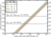Fig. 9.

Relation between the tidal synchronization timescale in a BH-WR binary and the delay time (between the formation and the merger) of the corresponding BBH system plotted for several different mass ratios q = M_WR/M_BH, using Eq. (14) from Kushnir et al. (2016). Tidal interactions can efficiently spin-up the WR star only if the synchronization timescale is shorter than the BH-WR binary lifetime t_BH-WR. The two dashed horizontal lines mark two different values of t_BH-WR: roughly the maximum WR lifetime ∼ 3 × 10⁵ yr, assumed by several authors (e.g., Kushnir et al. 2016; Hotokezaka & Piran 2017a; Piran & Hotokezaka 2018), and a significantly smaller value t_BH-WR = 3 × 10³ yr which is more realistic in the case of the CE channel at low metallicity.

4.5. Common-envelope ejection in BH-LMXB progenitors

Most of the known Galactic BHs reside in BH-LMXBs in which the companion is typically a MS star with M ≲ 1 M_⊙ and the orbital period is very short (usually < 1 day) (Casares & Jonker 2014; Tetarenko et al. 2016). The formation of such systems is a long-standing puzzle. Given the extreme mass ratio and small separation of BH-LMXBs, their progenitors have most likely evolved through a CE phase. However, it was argued by several authors on the basis of energy budget considerations that a secondary of only ≲1.5 M_⊙ would not be able to provide enough energy to unbind the envelope of a massive BH progenitor (Portegies Zwart et al. 1997; Kalogera 1999; Podsiadlowski et al. 2003; Justham et al. 2006; Yungelson & Lasota 2008, although see Yungelson et al. 2006). This led to the suggestion of an extremely high CE efficiency, that is, a possibility of α_CE larger than 1 (even as high as a few tens in the case of BH-LMXBs). This apparent violation of energy conservation could be interpreted as some unknown mechanism that is unaccounted for in the standard energy budget (e.g., Podsiadlowski et al. 2010). The assumption of α_CE larger than 1 has also made its way to population-synthesis models of compact binary mergers (e.g., Giacobbo & Mapelli 2018; Evans et al. 2020).

Interestingly, the binding energies of convective-envelope supergiants at advanced evolutionary stages (Fig. 1) described in detail in Sect. 3.4 are low enough to allow for a CE ejection even in the case of low-mass secondaries, without the need for α_CE > 1. Figure 10, which is similar to Fig. 2, shows CE ejectability in binaries with massive CE donors (M_ZAMS = 10 − 40 M_⊙) in which the companion is a 1.0 M_⊙ star, that is, potential BH-LMXB progenitors (depending on the minimum mass required for the formation of a BH). Post-CE separations a_post-CE, color-coded in the figure, follow from the energy budget described in Sect. 2.3 without the energy term from accretion (due to the stellar nature of the secondary). Separations within a_post-CE ≈ 4 − 10 R_⊙ agree well with the estimated separations of short-period BH-LMXB progenitors at the moment of the BH formation (Kalogera 1999; Repetto & Nelemans 2015). We note that at solar metallicity (the left panel) the decrease in envelope binding energy of convective-envelope giants is quenched for masses M_ZAMS ≳ 20 M_⊙ due to mass loss in our models (see also Podsiadlowski et al. 2003, and Fig. 1). If M_ZAMS ≈ 20 M_⊙ is the minimum mass required for the formation of a BH then none of the survivors in the left panel of Fig. 10 could be progenitors of BH-LMXBs. However, at the lower metallicity of Z = 0.4 Z_⊙ = 0.0068 the range of survivors extends to M_ZAMS = 25 M_⊙ (the right panel). Given that the average metallicity of the Milky Way stars is subsolar (e.g., Z = 0.0088 with the assumptions taken by Brott et al. 2011), Fig. 10 suggests that at least some of the Galactic BH-LMXBs could be formed through CE evolution without α_CE exceeding 1. Moreover, as pointed out by Yungelson et al. (2006), because mass-loss rates from massive stars are uncertain, it is possible that for a different set of mass-loss assumptions the range of CE survivors at the solar metallicity would extend to M_ZAMS > 20 M_⊙ as well (Smith 2014; Renzo et al. 2017). Finally, there might be islands of nonexplodability in the lower ZAMS mass range where some progenitors with M_ZAMS < 20 M_⊙ end their lives in failed explosions and produce BHs as well (O’Connor & Ott 2011; Ugliano et al. 2012; Ertl et al. 2016, 2020; Couch et al. 2020; Patton & Sukhbold 2020).

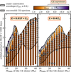Fig. 10.

Common-envelope ejectability in binaries with a massive donor (M_ZAMS = 10 − 40 M_⊙) and a low-mass secondary of 1.0 M_⊙, shown for two metallicites that are the most relevant for the Milky Way. Notation is the same as in Fig. 2, except that the Y-axis shows orbital period instead of the donor radius and the color indicates the post-CE orbital separation a_post-CE estimated from the energy budget (Sect. 2.3) without the accretion term ΔE_acc. Separations a_post-CE ≈ 4 − 10 R_⊙ are in line with the formation of the observed population of short-period BH-LMXBs (Kalogera 1999; Repetto & Nelemans 2015).

A separate question is whether the parameter space for CE ejection in Fig. 10 is large enough to produce the entire Galactic population of BH-LMXBs, something that population-synthesis models have been struggling with (e.g., Wiktorowicz et al. 2014). Notably, other formation channels for BH-LMXBs have also been suggested, for example intermediate-mass X-ray binaries with magnetic donors (Justham et al. 2006), formation in hierarchical triplets (Naoz et al. 2016), or dynamical formation through tidal capture in the field (Michaely & Perets 2016; Klencki et al. 2017).

4.6. Alternative scenario: partial envelope ejection followed by stable mass transfer

It is well known that the binding energy of a giant star is very sensitive to the exact location of the core-envelope boundary for CE ejection, that is, the bifurcation point (Dewi & Tauris 2000; Tauris & Dewi 2001; Ivanova et al. 2011a; De Marco et al. 2011; Kruckow et al. 2016). This is because most of the binding energy is stored is deep envelope layers close to the helium core (see Figs. 7e and 8e as well as Fig. 3 in Kruckow et al. 2016). As a result, moving the bifurcation point upwards by even a few percent of the total mass of a giant may reduce the envelope binding energy by an order of magnitude or even more. Here, following Ivanova et al. (2011a), the bifurcation point is assumed to be the maximum compression point M_cp within the H-burning shell (i.e., a local maximum of P/ρ), which in massive evolved stars corresponds very well to the point of steep composition gradient at the hydrogen abundance X_H ∼ 0.05 − 0.15. This is a standard assumption made across the recent literature (Xu & Li 2010; Loveridge et al. 2011; Wang et al. 2016; Kruckow et al. 2016).

Interestingly, in the envelope structure of a ∼35 M_⊙ convective giant at Z = 0.4 Z_⊙ in Fig. 8 (originally M_ZAMS = 47.5 M_⊙), the layers above the bifurcation point, located at M_cp ≈ 23 M_⊙, are still compressed at very compact radial coordinates R < 5 R_⊙; see Fig. 8c. These layers are helium rich (X_He ≈ 0.75) and extend out to mass coordinate M ≈ 26 M_⊙ at which point a steep density and composition gradient separates them from the loosely bound outer convective zone. As the model evolves from yellow to red profiles in Fig. 8c, when a significant amount of mass (∼10 M_⊙) is being lost in winds and the envelope becomes increasingly convective, the entire inner part of the star out to M ≈ 26 M_⊙ contracts slightly while the layers above are expanding. We find that such an envelope structure is characteristic of massive giants that become convective as a result of a rapid expansion during the HG phase. It is distinctively different from the structure of low-mass red giants or massive giants that develop outer convective zones at a more advanced evolutionary stage (e.g., Fig. 7), in which the convective zone can extend deep down close to the helium core and the maximum compression point is also a clear divergence point between the expanding and contracting parts of the star.

Given the compact size of layers above the helium core in the model from Fig. 8, it is possible to imagine a partial envelope ejection in which only the extended and loosely bound outer part of the envelop is ejected during the CE phase (at mass coordinates > 26 M_⊙). This would imply a bifurcation point located at ∼3 M_⊙ above the standard core-envelope boundary and a much lower envelope binding energy. For such a partial envelope ejection during inward spiralling of a CE to be possible, the helium-rich layers at the bottom of the envelope are likely required to remain compact during mass loss from the outer envelope layers taking place on the short CE timescale. Whether or not this is likely to happen needs to be confirmed with detailed stellar models. The first step has recently been carried out by Fragos et al. (2019), who, in their hydrodynamic 1D model of an inwardly spiralling NS inside the envelope of a 12 M_⊙ giant, found evidence for a CE ejection at a point when some of the envelope layers (∼0.3 − 0.5 M_⊙ with X_He ≈ 0.7 ) still remain on top of the helium core.

A separate but important question is what would happen with the system right after such a CE phase. One possibility is that the partially stripped donor star would re-expand again on the thermal timescale (∼100 − 1000 yr) leading to RLOF and another phase of mass transfer, as also discussed by Kruckow et al. (2016). Such behavior was found by Ivanova et al. (2011a) in models of stripped giants with remaining masses above the maximum compression point. Interestingly, Quast et al. (2019) recently showed that mass transfer from a massive giant that has been stripped down to its deep helium-enriched layers could be stable for significantly unequal mass ratios and proceed on a long nuclear timescale of core-helium burning (∼10⁵ yr) with a super-Eddington mass transfer rate. Taken together, these results support the idea of an alternative scenario to the classical evolution through a CE phase: a scenario in which a partial envelope ejection during the CE phase is followed by a long-lasting phase of stable mass transfer from a helium-enriched star, likely a blue supergiant, during which the system appears as a ULX.

It should be noted that the high mass-transfer stability in models by Quast et al. (2019) was obtained only if the giant was to lose most but not all of its envelope during the CE phase (≳90% in mass), at which point the helium-rich layers close to the helium core would be brought to the surface. At a first glance, this suggests that a certain level of fine-tuning is required. On the other hand, Quast et al. (2019) only explored synthetic models with simple internal abundance profiles. In real supergiants, depending on the size of the ICZ above the H-burning shell during the previous evolution, helium-rich layers (X_He ∼ 0.5 − 0.7) might extend to layers located significantly higher up inside the envelope (e.g., Figs. 7d and 8d). This could also be the case for accretors from a past mass transfer phase, especially if a significant amount of He-rich material was accreted. Such a structure could possibly support stable mass transfer evolution also when a different, smaller part of the H-rich envelope is ejected in the CE phase, especially at lower metallicity where stripped stars are more compact (Götberg et al. 2017, 2018; Klencki & Nelemans 2019; Laplace et al. 2020).

The final separation of a binary system once both a partial envelope ejection and a further mass transfer phase are concluded depends on the mass of the compact accretor, how conservative the second stable mass transfer is, and how much angular momentum is carried away in the nonaccreted matter. For instance, Fragos et al. (2019) estimated that a potential post-CE mass transfer phase would further decrease the separation in their binary of a 1.4 M_⊙ NS and a 3.2 M_⊙ stripped donor by a factor of ∼1.5. This, combined with the orbital shrinkage during the CE phase, can be translated into a single effective α_CE value. In the case of the system computed by Fragos et al. (2019), the authors estimated an effective ratio ΔE_grav/ΔE_orb = α_grav ≈ 5, which roughly translates to α_CE ≈ 2, essentially indicating a more likely CE ejection and binary survival compared to the classical picture of CE evolution in which the entire envelope is ejected immediately¹³. In the case of more massive accretors, such as for example typical stellar BHs, the orbital separation would likely decrease less or even increase as a result of a more equal mass ratio during the stable mass transfer phase, thus producing intermediate- rather than short-period systems. The fact that some of the recently ejected matter from the CE phase would likely still remain in the proximity of the system (e.g., as a circumbinary disk) makes predictions for the evolution of orbital parameters rather uncertain. The alleged noninteracting BH binary system with orbital period of ∼83 days and a companion ∼3 M_⊙ star discovered by Thompson et al. (2019), although see van den Heuvel & Tauris (2020) and Thompson et al. (2020), might be a product of such an evolution if a CE phase was initiated by the BH massive progenitor.

In summary, a different location of the bifurcation point in supergiant donors would result in lower envelope binding energies and could in principle allow for CE ejections even in the case of nonconvective donors. It would also lead to another phase of mass transfer after the end of the CE phase. It seems unlikely that close (merging) BBH systems could be the final product of such an evolution but if they were then the corresponding BBH merger rate could possibly be linked to the number density of observed ULX sources (Inoue et al. 2016; Finke & Razzaque 2017; Klencki & Nelemans 2019; Mondal et al. 2020).

5. Conclusions

We studied envelope binding energies in detailed massive stellar models at different evolutionary stages and metallicities in order to decipher the kinds of binaries with BH or NS accretors and supergiant donors that could realistically be expected to evolve through and survive a CE phase, thus making them potential progenitors of compact binary mergers. In pursuit of the most optimistic case, we assumed an extreme version of the CE energy budget, in which all the energy sources are fully efficient (orbital shrinkage, internal energy, recombination energy, energy from accretion), energy sinks are neglected (e.g., no energy loss in radiation), and the envelope acceleration is perfectly fine-tuned to the local escape velocity. We computed envelope binding energies from detailed stellar models of massive stars (M_ZAMS between 10 and 80 M_⊙) at six different metallicities from Z = 0.017 to 0.00017 and taking X_H = 0.1 criteria for the bifurcation point. We assumed that the CE evolution occurs in binaries with BH or NS accretors with mass ratios q = M_donor/M_accretor larger than q_crit; rad = 3.5 for radiative-envelope donors and q_crit; conv = 1.5 for convective-envelope donors. This choice might be optimistic in view of the recently found increased stability of mass transfer from massive giant donors (Ge et al. 2015; Pavlovskii et al. 2017). Our findings are summarized below.

− Envelope binding energy of a supergiant depends very strongly on not only the envelope type (convective vs. radiative) but also the evolutionary stage, which in turn is related to metallicity. The binding energy can decrease very significantly (by more than an order of magnitude) when the envelope becomes convective during core-helium burning or at a later evolutionary stage. However, a transition from a radiative to a convective state in an envelope of a rapidly expanding HG giant does not affect the binding energy nearly as significantly. As a result, through its impact on the radial expansion of massive giants, metallicity could have an indirect but very strong effect on the binding energies of convective-envelope giants and may be a crucial factor determining the fraction of systems surviving the CE phase. This conclusion depends on the presence of the ICZ during the HG phase. In Appendix A we provide fits to λ_CE values which can be used in population-synthesis calculations.

− Survival of the CE phase in binaries with BH or NS accretors is strongly limited to cases in which the donor star is a convective-envelope red supergiant. This is the case even under several optimistic assumptions working in favor of an easier CE ejection. Ultra-luminous X-ray sources with RSG donors might be the immediate progenitors of such CE events and subsequent compact binary mergers.

– If stars above ∼40 M_⊙ never expand to the RSG stage, as suggested by the empirical upper luminosity limit of RSGs at log(L/L_⊙)_RSG; max ≈ 5.7, then our result indicates an upper limit on the total BBH merger mass at about ∼50 M_⊙ and the primary BH mass at ∼25–30 M_⊙. This would be in tension with the CE channel being the origin of about half of the BBH mergers detected to date.

– Merger rates of compact binaries formed through the CE evolution might be severely overestimated in some of the recent population-synthesis models due to (a) extrapolation of λ_CE values fitted to M_ZAMS ≤ 20 M_⊙ models to obtain binding energies of much more massive stars (with M_ZAMS as high as 100 − 150 M_⊙) and (b) a practice of treating all core-helium burning stars as convective-envelope giants. The latter issue is likely partially responsible for the significantly higher formation rate of BBH mergers at low metallicity in these models.

– Lifetimes of close BH-WR systems (i.e., CE survivors) formed at low metallicity are typically very short (several thousand years), especially at Z ≤ 0.1 Z_⊙. Only those with the smallest orbital separations, producing BBH mergers with short delay times (≲30 Myr), are likely to experience any significant tidal spin-up of the WR star.

– Models at M_ZAMS ≲ 20 − 40 M_⊙ (depending on Z) remain RSGs at advanced evolutionary stages after the end of core-helium burning. Their envelopes can become deeply convective, leading to exceptionally small binding energies (λ_CE ∼ 1.0). For such donors, CE ejections appears energetically possible even for low-mass (1 M_⊙) MS accretors, making them potential progenitors of BH-LMXBs without the need for α_CE > 1.0.

– Envelopes of more massive stars (M_ZAMS ≳ 40 M_⊙), even if they reach the RSG stage, never become fully convective as their M_conv/M_env ratio does not exceed ∼0.7. In some models, layers above the helium core remain very compact (< 5 R_⊙) all the way up to a steep density gradient near the bottom of the convective envelope, which revives the question of the exact location of the core-envelope boundary in CE evolution. Eventual partial envelope ejection during the CE phase would likely lead to another, possibly stable and long-lasting phase of mass transfer.

– Because of its influence on the radial expansion of massive giants, metallicity affects the degree of internal mixing in deep envelope layers of supergiants. As a result, two RSGs similar in terms of mass, radius, and luminosity but of differing metallicity can have very different chemical profiles, density structures, and envelope binding energies. This might need to be taken into account when constructing RSG models for an input to hydrodynamic simulations of the CE phase.

¹

https://zenodo.org/record/3740578#.X1s2cnVfguw

²

We note that double-core CE evolution, when both the donor and the accretor are evolved giants, could also lead to the formation of compact binary mergers, although this channel requires both stars to be of very similar mass (e.g., Bethe & Brown 1998; Dewi et al. 2006).

³

Another issue with applying condensed polytropes to compute ζ_ad of convective donors as in Hjellming & Webbink (1987) is that in massive stars the superadiabatic layer is large enough to have to be taken into account and consequently the n = 3/2 polytrope is no longer a valid approximation of the entropy profile (Woods & Ivanova 2011; Pavlovskii & Ivanova 2015).

⁴

In the case of M_donor < 40 M_⊙, Pavlovskii et al. (2017) only tested mass ratios up to 4.

⁵

It is worth pointing out that Ivanova (2011b) emulated the CE evolution by studying adiabatic mass-loss sequences, thus preventing any thermal relaxation of the donor star. If, however, a CE phase is characterized by the thermal-timescale then the maximum compression point could move during the CE event with respect to its pre-CE location.

⁶

A mixing length of around 2 would probably result in better agreement with the observed RSG samples (Chun et al. 2018).

⁷

The fact that GENEVA models are hotter and more luminous during the MS is most likely a result of a higher efficiency of rotational mixing in GENEVA models compared to models computed by Klencki et al. (2020).

⁸

An exception are systems that become unstable on a shorter timescales due to Darwin instability (Darwin 1879; Eggleton & Kiseleva-Eggleton 2001), which could predominantly occur in cases of extreme mass ratios (q ≳ 10, Rasio 1995).

⁹

We note that the term intermediate convective zone sometimes also refers to a region of semiconvective and convective mixing that can take place above the H-burning core already during the MS; see for instance Farmer et al. (2016). Here, we follow a slightly different nomenclature (e.g., Langer et al. 1985; Kaiser et al. 2020).

¹⁰

An exception could be nondegenerate accretors, e.g., low-mass MS stars (Podsiadlowski et al. 2010).

¹¹

The low metallicity is likely favored regardless because of weaker stellar winds, but possibly to a lesser extent than in most population-synthesis models.

¹²

Whether λ_CE increases again once the outer convective envelope develops may depend on the evolutionary stage (see Sect. 3.4), with convective giants above a certain metallicity-dependent mass possibly maintaining λ_CE ≈ 0.01.

¹³

We note that α_CE from the notation of Fragos et al. (2019) is the same as α_grav in ours.

¹⁴

https://ftp.science.ru.nl/astro/jklencki/

¹⁵

See https://zenodo.org/record/3740578#.X1s21nVfguw for all the input MESA files.

Acknowledgments

We would like to thank the anonymous referee for a very thorough review and multiple useful comments and suggestions that helped to improve this work. The authors acknowledge support from the Netherlands Organisation for Scientific Research (NWO). It is a pleasure to acknowledge valuable discussions and suggestions from Alejandro Vigna-Góomez, Natasha Ivanova, Nadia Blagorodnova, Morgan MacLeod, Onno Pols, Kristhell López, Marianne Heida, Karel Temmink, Glenn-Michael Oomen, Raphael Hirschi, Stephen Justham, Selma de Mink, and Ilya Mandel.

References

Abadie, J., Abbott, B. P., Abbott, R., et al. 2010, Class. Quant. Grav., 27, 173001 [NASA ADS] [CrossRef] [Google Scholar]
Abbott, B. P., Abbott, R., Abbott, T. D., et al. 2016, Phys. Rev. Lett., 116, 061102 [Google Scholar]
Abbott, B. P., Abbott, R., Abbott, T. D., et al. 2019, Phys. Rev. X, 9, 031040 [Google Scholar]
Abbott, R., Abbott, T. D., Abraham, S., et al. 2020, ApJ, 896, L44 [Google Scholar]
Antonini, F., & Rasio, F. A. 2016, ApJ, 831, 187 [NASA ADS] [CrossRef] [Google Scholar]
Antonini, F., Toonen, S., & Hamers, A. S. 2017, ApJ, 841, 77 [NASA ADS] [CrossRef] [Google Scholar]
Arca-Sedda, M., & Gualandris, A. 2018, MNRAS, 477, 4423 [CrossRef] [Google Scholar]
Armitage, P. J., & Livio, M. 2000, ApJ, 532, 540 [CrossRef] [Google Scholar]
Askar, A., Szkudlarek, M., Gondek-Rosińska, D., Giersz, M., & Bulik, T. 2017, MNRAS, 464, L36 [NASA ADS] [CrossRef] [Google Scholar]
Barack, L., Cardoso, V., Nissanke, S., et al. 2019, Class. Quan. Grav., 36, 143001 [NASA ADS] [CrossRef] [Google Scholar]
Bavera, S. S., Fragos, T., Qin, Y., et al. 2020, A&A, 635, A97 [NASA ADS] [CrossRef] [EDP Sciences] [Google Scholar]
Begelman, M. C., King, A. R., & Pringle, J. E. 2006, MNRAS, 370, 399 [NASA ADS] [CrossRef] [Google Scholar]
Belczynski, K., Kalogera, V., Rasio, F. A., et al. 2008, ApJS, 174, 223 [NASA ADS] [CrossRef] [Google Scholar]
Belczynski, K., Dominik, M., Bulik, T., et al. 2010, ApJ, 715, L138 [NASA ADS] [CrossRef] [Google Scholar]
Belczynski, K., Bulik, T., Mandel, I., et al. 2013, ApJ, 764, 96 [NASA ADS] [CrossRef] [Google Scholar]
Belczynski, K., Holz, D. E., Bulik, T., & O’Shaughnessy, R. 2016, Nature, 534, 512 [NASA ADS] [CrossRef] [Google Scholar]
Belczynski, K., Klencki, J., Fields, C. E., et al. 2020, A&A, 636, A104 [CrossRef] [EDP Sciences] [Google Scholar]
Benson, R. S. 1970, PhD Thesis, University of California, Berkeley, USA [Google Scholar]
Bethe, H. A., & Brown, G. E. 1998, ApJ, 506, 780 [NASA ADS] [CrossRef] [Google Scholar]
Blagorodnova, N., Kotak, R., Polshaw, J., et al. 2017, ApJ, 834, 107 [NASA ADS] [CrossRef] [Google Scholar]
Böhm-Vitense, E. 1958, Z. Astrophys., 46, 108 [Google Scholar]
Braun, H., & Langer, N. 1995, A&A, 297, 483 [NASA ADS] [Google Scholar]
Breivik, K., Coughlin, S., Zevin, M., et al. 2020, ApJ, 898, 71 [CrossRef] [Google Scholar]
Britavskiy, N. E., Bonanos, A. Z., Herrero, A., et al. 2019, A&A, 631, A95 [CrossRef] [EDP Sciences] [Google Scholar]
Brott, I., de Mink, S. E., Cantiello, M., et al. 2011, A&A, 530, A115 [NASA ADS] [CrossRef] [EDP Sciences] [Google Scholar]
Bulik, T., Belczynski, K., & Prestwich, A. 2011, ApJ, 730, 140 [NASA ADS] [CrossRef] [Google Scholar]
Carpano, S., Pollock, A. M. T., Prestwich, A., et al. 2007, A&A, 466, L17 [NASA ADS] [CrossRef] [EDP Sciences] [Google Scholar]
Casares, J., & Jonker, P. G. 2014, Space Sci. Rev., 183, 223 [NASA ADS] [CrossRef] [Google Scholar]
Chen, X., & Han, Z. 2002, MNRAS, 335, 948 [NASA ADS] [CrossRef] [Google Scholar]
Chen, Y., Bressan, A., Girardi, L., et al. 2015, MNRAS, 452, 1068 [NASA ADS] [CrossRef] [Google Scholar]
Chruslinska, M., & Nelemans, G. 2019, MNRAS, 488, 5300 [NASA ADS] [Google Scholar]
Chruslinska, M., Belczynski, K., Klencki, J., & Benacquista, M. 2018, MNRAS, 474, 2937 [NASA ADS] [CrossRef] [Google Scholar]
Chruslinska, M., Nelemans, G., & Belczynski, K. 2019, MNRAS, 482, 5012 [Google Scholar]
Chun, S.-H., Yoon, S.-C., Jung, M.-K., Kim, D. U., & Kim, J. 2018, ApJ, 853, 79 [NASA ADS] [CrossRef] [Google Scholar]
Clayton, M., Podsiadlowski, P., Ivanova, N., & Justham, S. 2017, MNRAS, 470, 1788 [NASA ADS] [CrossRef] [Google Scholar]
Couch, S. M., Warren, M. L., & O’Connor, E. P. 2020, ApJ, 890, 127 [NASA ADS] [CrossRef] [Google Scholar]
Darwin, G. H. 1879, Proc. R. Soc. London, Ser. I, 29, 168 [Google Scholar]
Davies, B., & Dessart, L. 2019, MNRAS, 483, 887 [NASA ADS] [CrossRef] [Google Scholar]
Davies, B., Crowther, P. A., & Beasor, E. R. 2018, MNRAS, 478, 3138 [NASA ADS] [CrossRef] [Google Scholar]
Davis, P. J., Kolb, U., & Knigge, C. 2012, MNRAS, 419, 287 [NASA ADS] [CrossRef] [Google Scholar]
De, S., MacLeod, M., Everson, R. W., et al. 2020, ApJ, 897, 130 [CrossRef] [Google Scholar]
de Kool, M. 1990, ApJ, 358, 189 [NASA ADS] [CrossRef] [Google Scholar]
De Marco, O., Passy, J.-C., Moe, M., et al. 2011, MNRAS, 411, 2277 [NASA ADS] [CrossRef] [Google Scholar]
de Mink, S. E., & Belczynski, K. 2015, ApJ, 814, 58 [NASA ADS] [CrossRef] [Google Scholar]
de Mink, S. E., & Mandel, I. 2016, MNRAS, 460, 3545 [NASA ADS] [CrossRef] [Google Scholar]
de Mink, S. E., Pols, O. R., & Hilditch, R. W. 2007, A&A, 467, 1181 [NASA ADS] [CrossRef] [EDP Sciences] [Google Scholar]
de Mink, S. E., Langer, N., Izzard, R. G., Sana, H., & de Koter, A. 2013, ApJ, 764, 166 [NASA ADS] [CrossRef] [Google Scholar]
Dewi, J. D. M., & Tauris, T. M. 2000, A&A, 360, 1043 [NASA ADS] [Google Scholar]
Dewi, J. D. M., Podsiadlowski, P., & Sena, A. 2006, MNRAS, 368, 1742 [NASA ADS] [CrossRef] [Google Scholar]
Dominik, M., Belczynski, K., Fryer, C., et al. 2012, ApJ, 759, 52 [NASA ADS] [CrossRef] [Google Scholar]
Dray, L. M., & Tout, C. A. 2007, MNRAS, 376, 61 [NASA ADS] [CrossRef] [Google Scholar]
Edgar, R. 2004, New A Rev., 48, 843 [CrossRef] [Google Scholar]
Eggleton, P. P., & Kiseleva-Eggleton, L. 2001, ApJ, 562, 1012 [NASA ADS] [CrossRef] [Google Scholar]
Ekström, S., Georgy, C., Eggenberger, P., et al. 2012, A&A, 537, A146 [NASA ADS] [CrossRef] [EDP Sciences] [Google Scholar]
Eldridge, J. J., & Stanway, E. R. 2016, MNRAS, 462, 3302 [NASA ADS] [CrossRef] [Google Scholar]
Ertl, T., Janka, H. T., Woosley, S. E., Sukhbold, T., & Ugliano, M. 2016, ApJ, 818, 124 [NASA ADS] [CrossRef] [Google Scholar]
Ertl, T., Woosley, S. E., Sukhbold, T., & Janka, H. T. 2020, ApJ, 890, 51 [CrossRef] [Google Scholar]
Evans, F. A., Renzo, M., & Rossi, E. M. 2020, MNRAS, 497, 5344 [Google Scholar]
Fabrika, S. 2004, Astrophys. Space Phys. Res., 12, 1 [Google Scholar]
Farmer, R., Fields, C. E., Petermann, I., et al. 2016, ApJS, 227, 22 [NASA ADS] [CrossRef] [Google Scholar]
Farmer, R., Renzo, M., de Mink, S. E., Marchant, P., & Justham, S. 2019, ApJ, 887, 53 [CrossRef] [Google Scholar]
Farr, W. M., Stevenson, S., Miller, M. C., et al. 2017, Nature, 548, 426 [NASA ADS] [CrossRef] [Google Scholar]
Farr, B., Holz, D. E., & Farr, W. M. 2018, ApJ, 854, L9 [NASA ADS] [CrossRef] [Google Scholar]
Finke, J. D., & Razzaque, S. 2017, MNRAS, 472, 3683 [CrossRef] [Google Scholar]
Fragione, G., & Kocsis, B. 2019, MNRAS, 486, 4781 [CrossRef] [Google Scholar]
Fragione, G., Grishin, E., Leigh, N. W. C., Perets, H. B., & Perna, R. 2019, MNRAS, 488, 47 [CrossRef] [Google Scholar]
Fragos, T., Andrews, J. J., Ramirez-Ruiz, E., et al. 2019, ApJ, 883, L45 [NASA ADS] [CrossRef] [Google Scholar]
Ge, H., Hjellming, M. S., Webbink, R. F., Chen, X., & Han, Z. 2010, ApJ, 717, 724 [NASA ADS] [CrossRef] [Google Scholar]
Ge, H., Webbink, R. F., Chen, X., & Han, Z. 2015, ApJ, 812, 40 [NASA ADS] [CrossRef] [Google Scholar]
Georgy, C., Ekström, S., Eggenberger, P., et al. 2013, A&A, 558, A103 [NASA ADS] [CrossRef] [EDP Sciences] [Google Scholar]
Gerosa, D., Berti, E., O’Shaughnessy, R., et al. 2018, Phys. Rev. D, 98, 084036 [NASA ADS] [CrossRef] [Google Scholar]
Giacobbo, N., & Mapelli, M. 2018, MNRAS, 480, 2011 [NASA ADS] [CrossRef] [Google Scholar]
Giacobbo, N., & Mapelli, M. 2020, ApJ, 891, 141 [CrossRef] [Google Scholar]
Giacobbo, N., Mapelli, M., & Spera, M. 2018, MNRAS, 474, 2959 [NASA ADS] [CrossRef] [Google Scholar]
Ginat, Y. B., Glanz, H., Perets, H. B., Grishin, E., & Desjacques, V. 2020, MNRAS, 493, 4861 [CrossRef] [Google Scholar]
Götberg, Y., de Mink, S. E., & Groh, J. H. 2017, A&A, 608, A11 [NASA ADS] [CrossRef] [EDP Sciences] [Google Scholar]
Götberg, Y., de Mink, S. E., Groh, J. H., et al. 2018, A&A, 615, A78 [NASA ADS] [CrossRef] [EDP Sciences] [Google Scholar]
Gräfener, G., Owocki, S. P., & Vink, J. S. 2012, A&A, 538, A40 [NASA ADS] [CrossRef] [EDP Sciences] [Google Scholar]
Graziani, L., Schneider, R., Marassi, S., et al. 2020, MNRAS, 495, L81 [CrossRef] [Google Scholar]
Grevesse, N., Noels, A., & Sauval, A. J. 1996, ASP Conf. Ser., 99, 117 [Google Scholar]
Hamann, W. R., Koesterke, L., & Wessolowski, U. 1995, A&A, 299, 151 [Google Scholar]
Han, Z. 1998, MNRAS, 296, 1019 [NASA ADS] [CrossRef] [Google Scholar]
Han, Z., Podsiadlowski, P., & Eggleton, P. P. 1994, MNRAS, 270, 121 [NASA ADS] [CrossRef] [Google Scholar]
Heger, A., Fryer, C. L., Woosley, S. E., Langer, N., & Hartmann, D. H. 2003, ApJ, 591, 288 [NASA ADS] [CrossRef] [Google Scholar]
Heida, M., Torres, M. A. P., Jonker, P. G., et al. 2015, MNRAS, 453, 3510 [NASA ADS] [CrossRef] [Google Scholar]
Heida, M., Jonker, P. G., Torres, M. A. P., et al. 2016, MNRAS, 459, 771 [NASA ADS] [CrossRef] [Google Scholar]
Heida, M., Lau, R. M., Davies, B., et al. 2019a, ApJ, 883, L34 [CrossRef] [Google Scholar]
Heida, M., Harrison, F. A., Brightman, M., et al. 2019b, ApJ, 871, 231 [CrossRef] [Google Scholar]
Hellings, P. 1983, Ap&SS, 96, 37 [NASA ADS] [CrossRef] [Google Scholar]
Hellings, P. 1984, Ap&SS, 104, 83 [NASA ADS] [CrossRef] [Google Scholar]
Higgins, E. R., & Vink, J. S. 2019, A&A, 622, A50 [NASA ADS] [CrossRef] [EDP Sciences] [Google Scholar]
Higgins, E. R., & Vink, J. S. 2020, A&A, 635, A175 [NASA ADS] [CrossRef] [EDP Sciences] [Google Scholar]
Hillwig, T. C., & Gies, D. R. 2008, ApJ, 676, L37 [NASA ADS] [CrossRef] [Google Scholar]
Hjellming, M. S., & Webbink, R. F. 1987, ApJ, 318, 794 [NASA ADS] [CrossRef] [Google Scholar]
Hotokezaka, K., & Piran, T. 2017a, ApJ, submitted [arXiv:1707.08978] [Google Scholar]
Hotokezaka, K., & Piran, T. 2017b, ApJ, 842, 111 [NASA ADS] [CrossRef] [Google Scholar]
Houck, J. C., & Chevalier, R. A. 1991, ApJ, 376, 234 [CrossRef] [Google Scholar]
Howitt, G., Stevenson, S., Vigna-Gómez, A., et al. 2020, MNRAS, 492, 3229 [CrossRef] [Google Scholar]
Humphreys, R. M., & Davidson, K. 1979, ApJ, 232, 409 [NASA ADS] [CrossRef] [Google Scholar]
Humphreys, R. M., & Davidson, K. 1994, PASP, 106, 1025 [NASA ADS] [CrossRef] [Google Scholar]
Hurley, J. R., Pols, O. R., & Tout, C. A. 2000, MNRAS, 315, 543 [NASA ADS] [CrossRef] [Google Scholar]
Hurley, J. R., Tout, C. A., & Pols, O. R. 2002, MNRAS, 329, 897 [NASA ADS] [CrossRef] [Google Scholar]
Iben, I. J., & Livio, M. 1993, PASP, 105, 1373 [Google Scholar]
Iben, I. J., & Tutukov, A. V. 1984, ApJ, 284, 719 [NASA ADS] [CrossRef] [Google Scholar]
Inoue, Y., Tanaka, Y. T., & Isobe, N. 2016, MNRAS, 461, 4329 [NASA ADS] [CrossRef] [Google Scholar]
Ivanova, N. 2011a, ASP Conf. Ser., 447, 91 [Google Scholar]
Ivanova, N. 2011b, ApJ, 730, 76 [NASA ADS] [CrossRef] [Google Scholar]
Ivanova, N., & Podsiadlowski, P. 2003, in From Twilight to Highlight: The Physics of Supernovae, eds. W. Hillebrandt, & B. Leibundgut, 19 [Google Scholar]
Ivanova, N., & Taam, R. E. 2004, ApJ, 601, 1058 [NASA ADS] [CrossRef] [Google Scholar]
Ivanova, N., & Chaichenets, S. 2011, ApJ, 731, L36 [NASA ADS] [CrossRef] [Google Scholar]
Ivanova, N., Justham, S., Avendano Nandez, J. L., & Lombardi, J. C. 2013a, Science, 339, 433 [NASA ADS] [CrossRef] [Google Scholar]
Ivanova, N., Justham, S., Chen, X., et al. 2013b, A&ARv, 21, 59 [Google Scholar]
Ivanova, N., Justham, S., & Podsiadlowski, P. 2015, MNRAS, 447, 2181 [NASA ADS] [CrossRef] [Google Scholar]
Jiang, Y.-F., Cantiello, M., Bildsten, L., Quataert, E., & Blaes, O. 2015, ApJ, 813, 74 [Google Scholar]
Jiang, Y.-F., Cantiello, M., Bildsten, L., et al. 2018, Nature, 561, 498 [NASA ADS] [CrossRef] [Google Scholar]
Justham, S., Rappaport, S., & Podsiadlowski, P. 2006, MNRAS, 366, 1415 [NASA ADS] [CrossRef] [Google Scholar]
Justham, S., Podsiadlowski, P., & Vink, J. S. 2014, ApJ, 796, 121 [NASA ADS] [CrossRef] [Google Scholar]
Kaiser, E. A., Hirschi, R., Arnett, W. D., et al. 2020, MNRAS, 496, 1967 [CrossRef] [Google Scholar]
Kalogera, V. 1999, ApJ, 521, 723 [NASA ADS] [CrossRef] [Google Scholar]
King, A. R., & Ritter, H. 1999, MNRAS, 309, 253 [NASA ADS] [CrossRef] [Google Scholar]
King, A. R., Taam, R. E., & Begelman, M. C. 2000, ApJ, 530, L25 [NASA ADS] [CrossRef] [Google Scholar]
Klencki, J., & Nelemans, G. 2019, IAU Symp., 346, 417 [Google Scholar]
Klencki, J., Wiktorowicz, G., Gładysz, W., & Belczynski, K. 2017, MNRAS, 469, 3088 [NASA ADS] [CrossRef] [Google Scholar]
Klencki, J., Moe, M., Gladysz, W., et al. 2018, A&A, 619, A77 [NASA ADS] [CrossRef] [EDP Sciences] [Google Scholar]
Klencki, J., Nelemans, G., Istrate, A. G., & Pols, O. 2020, A&A, 638, A55 [NASA ADS] [CrossRef] [EDP Sciences] [Google Scholar]
Kochanek, C. S., Adams, S. M., & Belczynski, K. 2014, MNRAS, 443, 1319 [NASA ADS] [CrossRef] [PubMed] [Google Scholar]
Kolb, U., & Ritter, H. 1990, A&A, 236, 385 [NASA ADS] [Google Scholar]
Kruckow, M. U., Tauris, T. M., Langer, N., et al. 2016, A&A, 596, A58 [NASA ADS] [CrossRef] [EDP Sciences] [Google Scholar]
Kruckow, M. U., Tauris, T. M., Langer, N., Kramer, M., & Izzard, R. G. 2018, MNRAS, 481, 1908 [NASA ADS] [CrossRef] [Google Scholar]
Kulkarni, S. R., Ofek, E. O., Rau, A., et al. 2007, Nature, 447, 458 [Google Scholar]
Kushnir, D., Zaldarriaga, M., Kollmeier, J. A., & Waldman, R. 2016, MNRAS, 462, 844 [NASA ADS] [CrossRef] [Google Scholar]
Langer, N., El Eid, M. F., & Fricke, K. J. 1985, A&A, 145, 179 [NASA ADS] [Google Scholar]
Laplace, E., Götberg, Y., de Mink, S. E., Justham, S., & Farmer, R. 2020, A&A, 637, A6 [CrossRef] [EDP Sciences] [Google Scholar]
Lau, R. M., Heida, M., Walton, D. J., et al. 2019, ApJ, 878, 71 [CrossRef] [Google Scholar]
Leung, S.-C., Nomoto, K., & Blinnikov, S. 2019, ApJ, 887, 72 [NASA ADS] [CrossRef] [Google Scholar]
Levesque, E. M., Massey, P., Olsen, K. A. G., et al. 2006, ApJ, 645, 1102 [NASA ADS] [CrossRef] [Google Scholar]
Liu, J.-F., Bregman, J. N., Bai, Y., Justham, S., & Crowther, P. 2013, Nature, 503, 500 [NASA ADS] [CrossRef] [Google Scholar]
Livio, M., & Soker, N. 1988, ApJ, 329, 764 [NASA ADS] [CrossRef] [Google Scholar]
Lommen, D., Yungelson, L., van den Heuvel, E., Nelemans, G., & Portegies Zwart, S. 2005, A&A, 443, 231 [NASA ADS] [CrossRef] [EDP Sciences] [Google Scholar]
López, K. M., Heida, M., Jonker, P. G., et al. 2020, MNRAS, 497, 917 [CrossRef] [Google Scholar]
Loveridge, A. J., van der Sluys, M. V., & Kalogera, V. 2011, ApJ, 743, 49 [NASA ADS] [CrossRef] [Google Scholar]
Lubow, S. H., & Shu, F. H. 1975, ApJ, 198, 383 [NASA ADS] [CrossRef] [Google Scholar]
MacLeod, M., & Loeb, A. 2020a, ApJ, 895, 29 [CrossRef] [Google Scholar]
MacLeod, M., & Loeb, A. 2020b, ApJ, 893, 106 [CrossRef] [Google Scholar]
MacLeod, M., & Ramirez-Ruiz, E. 2015a, ApJ, 803, 41 [NASA ADS] [CrossRef] [Google Scholar]
MacLeod, M., & Ramirez-Ruiz, E. 2015b, ApJ, 798, L19 [NASA ADS] [CrossRef] [Google Scholar]
MacLeod, M., Antoni, A., Murguia-Berthier, A., Macias, P., & Ramirez-Ruiz, E. 2017, ApJ, 838, 56 [NASA ADS] [CrossRef] [Google Scholar]
MacLeod, M., Ostriker, E. C., & Stone, J. M. 2018a, ApJ, 868, 136 [NASA ADS] [CrossRef] [Google Scholar]
MacLeod, M., Ostriker, E. C., & Stone, J. M. 2018b, ApJ, 863, 5 [NASA ADS] [CrossRef] [Google Scholar]
Mandel, I., & de Mink, S. E. 2016, MNRAS, 458, 2634 [NASA ADS] [CrossRef] [Google Scholar]
Mandel, I., & Fragos, T. 2020, ApJ, 895, L28 [CrossRef] [Google Scholar]
Mapelli, M., & Giacobbo, N. 2018, MNRAS, 479, 4391 [NASA ADS] [CrossRef] [Google Scholar]
Mapelli, M., Giacobbo, N., Ripamonti, E., & Spera, M. 2017, MNRAS, 472, 2422 [NASA ADS] [CrossRef] [Google Scholar]
Marchant, P., Langer, N., Podsiadlowski, P., Tauris, T. M., & Moriya, T. J. 2016, A&A, 588, A50 [NASA ADS] [CrossRef] [EDP Sciences] [Google Scholar]
Marchant, P., Langer, N., Podsiadlowski, P., et al. 2017, A&A, 604, A55 [NASA ADS] [CrossRef] [EDP Sciences] [Google Scholar]
Mauerhan, J. C., Van Dyk, S. D., Johansson, J., et al. 2018, MNRAS, 473, 3765 [NASA ADS] [CrossRef] [Google Scholar]
McKernan, B., Ford, K. E. S., Bellovary, J., et al. 2018, ApJ, 866, 66 [Google Scholar]
Mennekens, N., & Vanbeveren, D. 2014, A&A, 564, A134 [NASA ADS] [CrossRef] [EDP Sciences] [Google Scholar]
Meyer, F., & Meyer-Hofmeister, E. 1979, A&A, 78, 167 [NASA ADS] [Google Scholar]
Michaely, E., & Perets, H. B. 2016, MNRAS, 458, 4188 [NASA ADS] [CrossRef] [Google Scholar]
Misra, D., Fragos, T., Tauris, T., Zapartas, E., & Aguilera-Dena, D. R. 2020, A&A, 642, A174 [CrossRef] [EDP Sciences] [Google Scholar]
Mondal, S., Belczyński, K., Wiktorowicz, G., Lasota, J.-P., & King, A. R. 2020, MNRAS, 491, 2747 [Google Scholar]
Murguia-Berthier, A., MacLeod, M., Ramirez-Ruiz, E., Antoni, A., & Macias, P. 2017, ApJ, 845, 173 [NASA ADS] [CrossRef] [Google Scholar]
Nandez, J. L. A., & Ivanova, N. 2016, MNRAS, 460, 3992 [NASA ADS] [CrossRef] [Google Scholar]
Nandez, J. L. A., Ivanova, N., & Lombardi, J. C. J. 2015, MNRAS, 450, L39 [NASA ADS] [CrossRef] [Google Scholar]
Naoz, S., Fragos, T., Geller, A., Stephan, A. P., & Rasio, F. A. 2016, ApJ, 822, L24 [NASA ADS] [CrossRef] [Google Scholar]
Neijssel, C. J., Vigna-Gómez, A., Stevenson, S., et al. 2019, MNRAS, 490, 3740 [NASA ADS] [CrossRef] [Google Scholar]
Nelemans, G., Verbunt, F., Yungelson, L. R., & Portegies Zwart, S. F. 2000, A&A, 360, 1011 [NASA ADS] [Google Scholar]
Nelemans, G., Yungelson, L. R., Portegies Zwart, S. F., & Verbunt, F. 2001, A&A, 365, 491 [NASA ADS] [CrossRef] [EDP Sciences] [Google Scholar]
Neo, S., Miyaji, S., Nomoto, K., & Sugimoto, D. 1977, PASJ, 29, 249 [NASA ADS] [Google Scholar]
Neugent, K. F., Massey, P., Georgy, C., et al. 2020, ApJ, 889, 44 [CrossRef] [Google Scholar]
Nieuwenhuijzen, H., & de Jager, C. 1990, A&A, 231, 134 [NASA ADS] [Google Scholar]
O’Connor, E., & Ott, C. D. 2011, ApJ, 730, 70 [NASA ADS] [CrossRef] [Google Scholar]
Ohlmann, S. T., Röpke, F. K., Pakmor, R., & Springel, V. 2016, ApJ, 816, L9 [NASA ADS] [CrossRef] [Google Scholar]
O’Shaughnessy, R., Gerosa, D., & Wysocki, D. 2017, Phys. Rev. Lett., 119, 011101 [NASA ADS] [CrossRef] [Google Scholar]
Paczynski, B. 1976, IAU Symp., 73, 75 [NASA ADS] [EDP Sciences] [Google Scholar]
Passy, J.-C., Herwig, F., & Paxton, B. 2012, ApJ, 760, 90 [NASA ADS] [CrossRef] [Google Scholar]
Patton, R. A., & Sukhbold, T. 2020, MNRAS, 499, 2803 [CrossRef] [Google Scholar]
Pavlovskii, K., & Ivanova, N. 2015, MNRAS, 449, 4415 [NASA ADS] [CrossRef] [Google Scholar]
Pavlovskii, K., Ivanova, N., Belczynski, K., & Van, K. X. 2017, MNRAS, 465, 2092 [NASA ADS] [CrossRef] [Google Scholar]
Paxton, B., Bildsten, L., Dotter, A., et al. 2011, ApJS, 192, 3 [Google Scholar]
Paxton, B., Cantiello, M., Arras, P., et al. 2013, ApJS, 208, 4 [NASA ADS] [CrossRef] [Google Scholar]
Paxton, B., Marchant, P., Schwab, J., et al. 2015, ApJS, 220, 15 [Google Scholar]
Paxton, B., Schwab, J., Bauer, E. B., et al. 2018, ApJS, 234, 34 [NASA ADS] [CrossRef] [EDP Sciences] [Google Scholar]
Paxton, B., Smolec, R., Schwab, J., et al. 2019, ApJS, 243, 10 [NASA ADS] [CrossRef] [PubMed] [Google Scholar]
Piran, T., & Hotokezaka, K. 2018, ArXiv e-prints [arXiv:1807.01336] [Google Scholar]
Podsiadlowski, P. 2001, ASP Conf. Ser., 229, 239 [Google Scholar]
Podsiadlowski, P., Rappaport, S., & Han, Z. 2003, MNRAS, 341, 385 [NASA ADS] [CrossRef] [Google Scholar]
Podsiadlowski, P., Ivanova, N., Justham, S., & Rappaport, S. 2010, MNRAS, 406, 840 [NASA ADS] [Google Scholar]
Pols, O. R. 1994, A&A, 290, 119 [Google Scholar]
Popham, R., & Narayan, R. 1991, ApJ, 370, 604 [NASA ADS] [CrossRef] [Google Scholar]
Portegies Zwart, S. 2013, MNRAS, 429, L45 [NASA ADS] [Google Scholar]
Portegies Zwart, S. F., Verbunt, F., & Ergma, E. 1997, A&A, 321, 207 [Google Scholar]
Quast, M., Langer, N., & Tauris, T. M. 2019, A&A, 628, A19 [NASA ADS] [CrossRef] [EDP Sciences] [Google Scholar]
Rasio, F. A. 1995, ApJ, 444, L41 [NASA ADS] [CrossRef] [Google Scholar]
Renzo, M., Ott, C. D., Shore, S. N., & de Mink, S. E. 2017, A&A, 603, A118 [NASA ADS] [CrossRef] [EDP Sciences] [Google Scholar]
Renzo, M., Farmer, R. J., Justham, S., et al. 2020, MNRAS, 493, 4333 [CrossRef] [Google Scholar]
Repetto, S., & Nelemans, G. 2015, MNRAS, 453, 3341 [NASA ADS] [CrossRef] [Google Scholar]
Ricker, P. M., & Taam, R. E. 2012, ApJ, 746, 74 [NASA ADS] [CrossRef] [Google Scholar]
Ricker, P. M., Timmes, F. X., Taam, R. E., & Webbink, R. F. 2019, IAU Symp., 346, 449 [Google Scholar]
Rodriguez, C. L., Haster, C.-J., Chatterjee, S., Kalogera, V., & Rasio, F. A. 2016, ApJ, 824, L8 [NASA ADS] [CrossRef] [Google Scholar]
Samsing, J. 2018, Phys. Rev. D, 97, 103014 [NASA ADS] [CrossRef] [Google Scholar]
Sanyal, D., Grassitelli, L., Langer, N., & Bestenlehner, J. M. 2015, A&A, 580, A20 [NASA ADS] [CrossRef] [EDP Sciences] [Google Scholar]
Sanyal, D., Langer, N., Szécsi, D., Yoon, S., & Grassitelli, L. 2017, A&A, 597, A71 [NASA ADS] [CrossRef] [EDP Sciences] [Google Scholar]
Schneider, F. R. N., Izzard, R. G., Langer, N., & de Mink, S. E. 2015, ApJ, 805, 20 [Google Scholar]
Schootemeijer, A., Langer, N., Grin, N. J., & Wang, C. 2019, A&A, 625, A132 [NASA ADS] [CrossRef] [EDP Sciences] [Google Scholar]
Shiber, S., Iaconi, R., De Marco, O., & Soker, N. 2019, MNRAS, 488, 5615 [CrossRef] [Google Scholar]
Shu, F. H., & Lubow, S. H. 1981, ARA&A, 19, 277 [NASA ADS] [CrossRef] [Google Scholar]
Smith, N. 2014, ARA&A, 52, 487 [NASA ADS] [CrossRef] [MathSciNet] [Google Scholar]
Smith, N., Li, W., Silverman, J. M., Ganeshalingam, M., & Filippenko, A. V. 2011, MNRAS, 415, 773 [NASA ADS] [CrossRef] [Google Scholar]
Smith, N., Andrews, J. E., Van Dyk, S. D., et al. 2016, MNRAS, 458, 950 [NASA ADS] [CrossRef] [Google Scholar]
Soberman, G. E., Phinney, E. S., & van den Heuvel, E. P. J. 1997, A&A, 327, 620 [NASA ADS] [Google Scholar]
Soker, N. 2015, ApJ, 800, 114 [NASA ADS] [CrossRef] [Google Scholar]
Soker, N., & Tylenda, R. 2003, ApJ, 582, L105 [NASA ADS] [CrossRef] [Google Scholar]
Stevenson, S., Vigna-Gómez, A., Mandel, I., et al. 2017, Nat. Commun., 8, 14906 [NASA ADS] [CrossRef] [Google Scholar]
Stone, N. C., Metzger, B. D., & Haiman, Z. 2017, MNRAS, 464, 946 [NASA ADS] [CrossRef] [Google Scholar]
Tauris, T. M., & Dewi, J. D. M. 2001, A&A, 369, 170 [NASA ADS] [CrossRef] [EDP Sciences] [Google Scholar]
Tauris, T. M., & van den Heuvel, E. P. J. 2006, Formation and Evolution of Compact Stellar X-ray Sources (UK: Cambridge University Press), 39, 623 [Google Scholar]
Tauris, T. M., van den Heuvel, E. P. J., & Savonije, G. J. 2000, ApJ, 530, L93 [NASA ADS] [CrossRef] [PubMed] [Google Scholar]
Tauris, T. M., Kramer, M., Freire, P. C. C., et al. 2017, ApJ, 846, 170 [NASA ADS] [CrossRef] [Google Scholar]
Tetarenko, B. E., Bahramian, A., Arnason, R. M., et al. 2016, ApJ, 825, 10 [NASA ADS] [CrossRef] [Google Scholar]
The LIGO Scientific Collaboration, & the Virgo Collaboration (Abbott, R., et al.) 2020a, Phys. Rev. D, 102, 043015 [CrossRef] [Google Scholar]
The LIGO Scientific Collaboration, & the Virgo Collaboration (Abbott, R., et al.) 2020b, Phys. Rev. Lett., 125, 101102 [CrossRef] [Google Scholar]
Thompson, T. A., Kochanek, C. S., Stanek, K. Z., et al. 2019, Science, 366, 637 [NASA ADS] [CrossRef] [Google Scholar]
Thompson, T. A., Kochanek, C. S., Stanek, K. Z., et al. 2020, Science, 368, eaba4356 [CrossRef] [Google Scholar]
Tout, C. A., Aarseth, S. J., Pols, O. R., & Eggleton, P. P. 1997, MNRAS, 291, 732 [NASA ADS] [Google Scholar]
Tutukov, A., & Yungelson, L. 1979, IAU Symp., 83, 401 [Google Scholar]
Tylenda, R., Hajduk, M., Kamiński, T., et al. 2011, A&A, 528, A114 [NASA ADS] [CrossRef] [EDP Sciences] [Google Scholar]
Ugliano, M., Janka, H.-T., Marek, A., & Arcones, A. 2012, ApJ, 757, 69 [NASA ADS] [CrossRef] [Google Scholar]
Ulmer, A., & Fitzpatrick, E. L. 1998, ApJ, 504, 200 [NASA ADS] [CrossRef] [Google Scholar]
Vanbeveren, D. 1991, A&A, 252, 159 [NASA ADS] [Google Scholar]
Vanbeveren, D., De Loore, C., & Van Rensbergen, W. 1998, A&ARv, 9, 63 [Google Scholar]
Vanbeveren, D., Mennekens, N., Van Rensbergen, W., & De Loore, C. 2013, A&A, 552, A105 [NASA ADS] [CrossRef] [EDP Sciences] [Google Scholar]
van den Heuvel, E. P. J. 1976, IAU Symp., 73, 35 [Google Scholar]
van den Heuvel, E. P. J. 1994, A&A, 291, L39 [NASA ADS] [Google Scholar]
van den Heuvel, E. P. J., & Tauris, T. M. 2020, Science, 368, eaba3282 [CrossRef] [Google Scholar]
van den Heuvel, E. P. J., Portegies Zwart, S. F., & de Mink, S. E. 2017, MNRAS, 471, 4256 [NASA ADS] [CrossRef] [Google Scholar]
van Son, L. A. C., De Mink, S. E., Broekgaarden, F. S., et al. 2020, ApJ, 897, 100 [CrossRef] [Google Scholar]
Venn, K. A. 1999, ApJ, 518, 405 [NASA ADS] [CrossRef] [Google Scholar]
Vigna-Gómez, A., Neijssel, C. J., Stevenson, S., et al. 2018, MNRAS, 481, 4009 [NASA ADS] [CrossRef] [Google Scholar]
Vigna-Gómez, A., MacLeod, M., Neijssel, C. J., et al. 2020, PASA, 37, e038 [CrossRef] [Google Scholar]
Vink, J. S., de Koter, A., & Lamers, H. J. G. L. M. 2001, A&A, 369, 574 [NASA ADS] [CrossRef] [EDP Sciences] [Google Scholar]
Voss, R., & Tauris, T. M. 2003, MNRAS, 342, 1169 [NASA ADS] [CrossRef] [Google Scholar]
Wang, C., Jia, K., & Li, X.-D. 2016, Res. Astron. Astrophys., 16, 126 [NASA ADS] [Google Scholar]
Webbink, R. F. 1984, ApJ, 277, 355 [NASA ADS] [CrossRef] [Google Scholar]
Wellstein, S., Langer, N., & Braun, H. 2001, A&A, 369, 939 [NASA ADS] [CrossRef] [EDP Sciences] [Google Scholar]
Wiktorowicz, G., Belczynski, K., & Maccarone, T. 2014, Binary Systems, their Evolution and Environments, 37 [Google Scholar]
Wiktorowicz, G., Sobolewska, M., Lasota, J.-P., & Belczynski, K. 2017, ApJ, 846, 17 [CrossRef] [Google Scholar]
Woods, T. E., & Ivanova, N. 2011, ApJ, 739, L48 [NASA ADS] [CrossRef] [Google Scholar]
Woosley, S. E. 2017, ApJ, 836, 244 [NASA ADS] [CrossRef] [Google Scholar]
Xu, X.-J., & Li, X.-D. 2010, ApJ, 716, 114 [NASA ADS] [CrossRef] [Google Scholar]
Yungelson, L. R., & Lasota, J. P. 2008, A&A, 488, 257 [NASA ADS] [CrossRef] [EDP Sciences] [Google Scholar]
Yungelson, L. R., Lasota, J. P., Nelemans, G., et al. 2006, A&A, 454, 559 [NASA ADS] [CrossRef] [EDP Sciences] [Google Scholar]
Zaldarriaga, M., Kushnir, D., & Kollmeier, J. A. 2018, MNRAS, 473, 4174 [NASA ADS] [CrossRef] [Google Scholar]
Zorotovic, M., Schreiber, M. R., Gänsicke, B. T., & Nebot Gómez-Morán, A. 2010, A&A, 520, A86 [NASA ADS] [CrossRef] [EDP Sciences] [Google Scholar]
Zorotovic, M., Schreiber, M. R., & Gänsicke, B. T. 2011, A&A, 536, A42 [NASA ADS] [CrossRef] [EDP Sciences] [Google Scholar]

Appendix A: Common-envelope binding energy parameter fits

To facilitate the use of our results for instance in population-synthesis studies, we provide fits to the λ parameter, which is commonly used to describe the binding energy of the envelope and relate it to the properties of the donor star in CE phase (see Eq. (4)). We fit log₁₀(λ) as a function of the radius of the giant donor star log₁₀(R) with a third-order polynomial:

$\begin{matrix} {log}_{10} (λ) = a_{i} {log}_{10} {(R / R_{⊙})}^{3} + b_{i} {log}_{10} {(R / R_{⊙})}^{2} \\ + c_{i} {log}_{10} (R / R_{⊙}) + d_{i} . 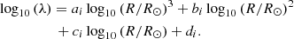\end{matrix}$ $\begin{aligned}&\log _{10}\left(\lambda \right) = a_{i} \log _{10}\left(R/R_{\odot } \right)^{3} + b_{i} \log _{10}\left(R/R_{\odot } \right)^{2} \nonumber \\ &\qquad \qquad \quad + c_{i} \log _{10}\left(R/R_{\odot } \right) + d_{i} .\end{aligned}$ (A.1)

The fit is divided in three ranges in R: coefficients with i = 1are applicable for R < R₁₂, those with i = 2 describe λ between R₁₂ < R < R₂₃, and those with i = 3 describe λ between R₂₃ < R < R_max. The fitted coefficients and ranges depend on the stellar mass and metallicity and are given online¹⁴ for each of the stellar models considered in this study. The example fit for 10, 20, and 40 M_⊙ models at Z = 0.2 Z_⊙ is shown in Fig. A.1. Below R₁₂ (cyan diamond in Fig. A.1), λ decreases monotonically as a function of radius. The relation starts to bend around R₁₂, when the mass fraction in the convective envelope increases (except for the highest stellar masses ≳50 M_⊙ at the highest metallicities considered in this study, see Sect. 3.1). In our fits, R₁₂ corresponds to the radius at which the effective temperature reaches the value below which at least 10% of the outer mass in a star becomes convective (see Fig. 6 in Klencki et al. 2020). The third range R₂₃ < R < R_max was introduced to improve the quality of the fit at the highest radii, where λ rapidly increases. For the most massive donors, the third range is not necessary (in those cases R₂₃ = R_max). Only the parts where the radius of the star increases beyond the largest radius reached during its previous evolution (relevant for the onset of the mass transfer and common envelope) are included in the fit.

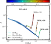Fig. A.1.

Polynomial fits to CE binding energy parameter (λ) as a function of radius shown for three example stellar models. The dashed lines in different colors indicate different ranges in which the fits have been made. The cyan diamond indicates the radius at which at least 10% of the mass of the envelope becomes convective, separating the first and the second fitted ranges. The background lines are colored according to the convective envelope mass fraction. The gray parts, where the radius was smaller than the maximum radius reached during the previous evolution, were not included in the fit.

Appendix B: Numerical robustness of models

B.1. The setup

In this section, we explore the numerical robustness of models from Klencki et al. (2020) (analyzed in this work) with respect to variations in spacial and temporal resolution. For an example of what an extended analysis of this kind could look like, we refer the reader to Farmer et al. (2016). Here, we mainly emphasize the model properties that are the most relevant in the context of CE evolution: the internal envelope structure and the envelope binding energy. MESA offers various controls to specify the mass (spacial) resolution of a model. One such parameter is mesh_delta_coeff which controls the global factor limiting the allowed change in stellar structure quantities between two adjacent cells. Lowering the value of mesh_delta_coeff leads to a higher number of cells (roughly by the same factor). The default value in MESA is mesh_delta_coeff = 1.0, whereas the default value for the models used in this work is mesh_delta_coeff = 0.8. Here, we also test mesh_delta_coeff = 0.6 (variation a). Another parameter controlling mass resolution is max_dq, which sets the maximum cell mass in units of the mass of the star. The default MESA value is max_dq = 10⁻², whereas the value used by Klencki et al. (2020) is max_dq = 10⁻³. Here, we also test max_dq = 3.3 × 10⁻⁴ (variation b). Apart from the two mesh controls mentioned above, models from Klencki et al. (2020) were computed with increased spacial resolution in regions with high H/He abundance gradients¹⁵.

As in the case of spacial resolution, MESA offers a large variety of parameters to control the time-step. One such parameter is varcontrol_target, which controls the maximum allowed relative change in stellar structure quantities between two subsequent time-steps (if the change is greater, then the time-steps needs to be reduced). The default value in MESA as well as in the models used in this work is varcontrol_target = 10⁻⁴. Here, we also explore a variation with varcontrol_target = 3.3 × 10⁻⁵ (variation c). Another relevant parameter is delta_HR_limit, which limits the change in position in the HR diagram between two subsequent time-steps. This is partifcularly important during the phase of evolution right after the end of MS when a star is rapidly expanding on a short thermal timescale, the core is contracting, and a convective zone is typically forming above the hydrogen burning shell (e.g., Langer et al. 1985; Schootemeijer et al. 2019; Klencki et al. 2020). In default MESA, this control is disabled, whereas the models used in this work take delta_HR_limit = 10⁻³. Here, we also test the value delta_HR_limit = 3.3 × 10⁻⁴ (variation d).

To get a better idea of the numerical robustness of our models, we computed four variations (a-d) described above, two with increased spacial resolution and two with increased temporal resolution. For each variation we computed stellar models at ten different masses: 12, 16, 20, 25, 32.5, 40, 47.5, 55, 65, and 80 M_⊙. We explored four different metallicities: 0.4, 0.2, 0.1, and 0.04 Z_⊙ (with Z_⊙ = 0.017).

B.2. Numerical robustness: envelope binding energies

In Fig. B.1, similarly to Fig. 1, we compare the envelope binding energies (plotted as a function of the stellar radius) in four numerical variations with the default models used throughout this study. We plot selected models at ten different masses and four different metallicities as listed above. Diamonds mark the onset of core-helium burning (Y_C drops below 0.975), crosses indicate central helium depletion (Y_C < 0.001). Shaded regions mark the area of uncertainty span by model variations, with interchanging colors to increase readability. We note that only the post-MS evolution is included in the figure. For simplicity, the end of MS is determined based on the helium core mass becoming nonzero in MESA but it coincides quite well with a condition X_C < 10⁻⁶ (i.e. core-hydrogen depletion).

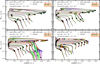Fig. B.1.

Comparison between the envelope binding energies E_bind of selected stellar models computed with the default assumptions (black line) and in four model variations with increased spacial or temporal resolution (see text for details), plotted as a function of the stellar radius. Selected stellar masses are 12, 16, 20, 25, 32.5, 40, 47.5, 55, 65, and 80 M_⊙. Each panel shows a different metallicity. Diamonds mark the onset of core-helium burning, crosses indicate central helium depletion. Shaded regions mark the area of uncertainty span by model variations, with interchanging colors to increase readability. We note that only the post-MS evolution is included in the figure. Differences between the models are likely mainly due to envelope inflation and density inversions in the outer envelopes; see text for details. None of the numerical difficulties affect the conclusions of this study.

There are three ways in which the numerically varied models are different from the default ones. First, there are clear discrepancies in the evolution of the most massive models right after the end of the MS (except for the lowest metallicity 0.04 Z_⊙). We find that these models are numerically not robust (not converged) in terms of their stellar radii at terminal-age MS (TAMS) and also during the final MS stages. For instance, numerical variations in the three most massive models at 0.4 Z_⊙ (55 M_⊙, 65 M_⊙, and 80 M_⊙) show changes in the TAMS radius as large as 100 − 200 R_⊙. Even larger is the numerical noise in the TAMS radius of the 80 M_⊙ models at 0.1 Z_⊙ (spread from ∼130 to 550 R_⊙) and, especially, the 80 M_⊙ models at 0.2 Z_⊙ metallicity (∼1000 − 1200 R_⊙ for models with increased spacial resolution, ∼550 R_⊙ otherwise). The problems arise due to envelope inflation which occurs in these models during late stages of MS (e.g., Gräfener et al. 2012; Sanyal et al. 2015, 2017) and poses a well-known numerical challenge for 1D stellar codes of computing extremely diluted radiation-dominated envelopes with a density inversion (see Sect. 7 in Paxton et al. 2013 and Appendix A in Klencki et al. 2020). Notably, it was shown that in 3D simulations the envelopes do not become as inflated as in 1D stellar models (i.e., the radius is smaller Jiang et al. 2018), which shows the limitations of 1D codes in computing the radii of very massive MS stars. In the context of the present study and CE ejectability, uncertainty in the final MS radii leads to uncertainty in the exact size and shape of the excluded MS area in Fig. 2.

Second, Fig. B.1 shows significant differences between the stellar radii of some of the models at the RSG stage (typically the more massive ones), when the star is already expanded to its almost largest radius and the outer convective zone is growing. Once again, during this part of the evolution a density inversion is particularly large, which leads to numerical difficulties. This is also when the superadiabatic layer, where the convection becomes supersonic and the mixing-length theory is outside its region of applicability, is the most extended. As such, paraphrasing Paxton et al. (2013), stellar radii of massive RSGs from any 1D stellar evolution calculation should be considered highly uncertain. Notably, much of the radius uncertainty is associated with the period of temporary contraction in models that reach the RSG stage before the onset of core-helium burning. In the context of binary evolution and a possibility of RLOF, this phase is not very relevant and does not affect out results. The more important is the uncertainty in the maximum radius reached during the phase of rapid HG expansion, which is just before the above-mentioned occasional contraction. In this case the numerical noise is less consequential: the typical radius variations are smaller than 5% with an exception of the 55 M_⊙ models at 0.1 Z_⊙ (∼10% uncertainty).

Apart from discrepancies in the stellar radius, some of the models at Z = 0.1 Z_⊙ show large numerical noise in the envelope binding energy E_bind during late evolutionary stages, when the envelope becomes deeply convective and the value of E_bind decreases significantly. This is due to variations in the exact location of the bifurcation point between these models (i.e., the boundary between the ejected envelope and the remaining remnant of the donor star during a CE phase), as we demonstrate below. This means that while the prediction of much lower binding energies of deeply convective RSGs at advanced stages of core-helium burning appears robust (and so does the prediction that CE ejection is possible for these donors), the exact values of E_bind for the loosely bound envelopes of these stars should be considered highly uncertain in our models.

Third, as indicated by different locations of diamonds and crosses between some of the model variations in Fig. B.1, stellar radius of a model during a transitory phase (onset or end of core-helium burning) is in some cases not numerically robust in our models. This likely has to do with the fact that stellar radii of blue supergiants are very sensitive to the exact abundance profile in the bottom envelope layers surrounding the hydrogen burning shell (e.g., Georgy et al. 2013; Klencki et al. 2020; Kaiser et al. 2020). The abundance pattern in this part of the star is a result of internal mixing which takes place shortly after the end of the MS and is notoriously difficult to compute in stellar models due to a abundance discontinuities (a step-like profile) left by semiconvection (Farmer et al. 2016).

It is important to stress that while the models used in this work are in some aspects not numerically robust, as revealed by Fig. B.1, the overall behavior of the binding energy as a function of radius (and therefore the convective-envelope mass fraction f_conv) is robust. In particular, numerical variations in the value of E_bind for radiative-envelope donors are never larger than 15% and typically below 10%, which is rather insignificant in view of various physical uncertainties in the energy-budget formalism for CE evolution (see Sect. 4.1). The numerical uncertainty of our models does not affect any of the results presented in Sects. 3.1 and 3.2 (at least within the scope explored above).

B.3. Numerical robustness: detailed internal structure

In Figs. B.3 and B.2 we take a look at numerical robustness of the internal structure of the two M_ZAMS = 47.5 M_⊙ models studied in detail in Sect. 3.4. Similarly to Figs. 7 and 8, with different colors we plot internal profiles selected based on their increasing depth of the outer convective zone f_conv (going from blue to red). We compare the default model (solid line) with numerical variations, investigating the helium abundance and the mass–radius profile. Vertical lines mark the bifurcation point for CE evolution.

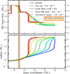Fig. B.2.

Comparison of the internal helium abundance and mass-radius profiles between the standard model (solid lines) and numerical variations with increased resolution (other lines), plotted for the case with M_ZAMS = 47.5 M_⊙ and 0.4 Z_⊙ analyzed in Sect. 3.4. As in Fig. 8, different colors correspond to different internal profiles of a model selected based on the depth of the outer convective zone (increasing as the color changes from blue to red). Vertical lines show the location of the bifurcation point for CE evolution.

None of the numerical variations in Fig. B.2 show any significant change with respect to our standard model. The largest variation in the bifurcation point location between models with different resolution is about 1.4% in mass and about 2% in radius.

The lower metallicity model Z = 0.1 Z_⊙ in Fig. B.3 on the other hand reveals two uncertainties. First, because of the uncertain radius of a core-helium burning blue/yellow supergiant for a given central helium abundance as discussed at the end of Appendix B.2, different models in Fig. B.3 reach the same outer convective zone depth at slightly different times. This is the most evident with the light-blue profiles, for which the total stellar mass is clearly different between model variations. The overall shape of each profile is unaffected.

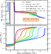Fig. B.3.

Same as Fig. B.2 but for a model at Z = 0.1 Z_⊙ metallicity (see also Fig. 7 in the main text).

Second, in the case of internal profiles of very deeply convective envelopes (the orange and red lines), there are some differences in the slope of the mass–radius profile near the bifurcation point (especially the model with varcontrol_target = 3.3 × 10⁻⁵ compared to all the others). While these variations do not lead to any significant uncertainty in the mass coordinate of the bifurcation point (which does not vary by more than 1.5%) they do result in the radial coordinate being up to ∼30% larger in the variation with max_dq = 3.3 × 10⁻⁴ (0.9 R_⊙ instead of 0.7 R_⊙, roughly). This propagates to very noticeable differences in the late envelope binding energy evolution of some of the Z = 0.1 Z_⊙ models (see Fig. B.1) when their envelopes become the most expanded, the most deeply convective, and the least gravitationally bound.

Most importantly, the overall shape of internal profiles in Figs. B.3 and B.2 is unaffected by an increase in resolution, and the results presented in Sect. 3.4 are numerically robust.

B.4. Numerical robustness: HR diagram at Z = 0.2 Z_⊙

In Fig. B.4, similarly to Fig. 6, we plot an HR diagram with selected models at 0.2 Z_⊙ metallicity (SMC-like). We compare models computed with increased resolution (various colors) to the standard models used in this work (in black). See the figure caption for a description of the symbols. None of the numerical variations show very significant discrepancies with respect to the default model. One noticeable difference is in the location of the core-helium burning phase in the HR diagram (marked with circular dots). In particular, the 12 M_⊙ model experiences a blue loop in a variation with max_dq = 3.3 × 10⁻⁴ (increased minimal cell size). These differences do not affect the envelope binding energies or the results on CE ejectability. As discussed in Appendix B.2, numerical tests reveal that the sizes of MS stars with inflated envelopes are not a robust prediction of our models, showing variations for the most massive models in metallicities Z ≥ 0.1 Z_⊙. This can also be seen in Fig. B.4 in the form of a chaotic behavior of the 80 M_⊙ model in the final stages of the MS.

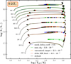Fig. B.4.

HR diagram with selected models at 0.2 Z_⊙ metallicity (SMC-like). We compare models computed with increased resolution (various colors) to the standard models used in this work (in black). Diamonds mark the terminal-age MS, dots mark the position of the star taken every 50 000 years during its post-MS evolution, white crosses mark the end of core-helium burning, whereas red stars mark the end of central carbon burning.

Appendix C: Additional figures

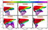Fig. C.1.

Same as Fig. 1 but with all the masses in our grid (30 models between 10 and 80 M_⊙ for each metallicity).

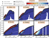Fig. C.2.

Same as Fig. 2 with the companion being a 2 M_⊙ NS. The parameter space for CE ejections is limited to cases in which the envelope binding energies have decreased significantly due to the donor becoming a convective-envelope giant at an advanced evolutionary stage.

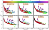Fig. C.3.

Same as Fig. 1, but showing the evolution of λ_CE parameter instead of the envelope binding energy. Diamonds indicate the onset of core-helium burning, crosses indicate the end of core-helium burning.

All Figures

Fig. 1.

Envelope binding energies E_bind of massive giants (i.e., the post-MS part of the evolution) as a function of their radius for six different metallicities (selected models from Klencki et al. 2020). See Fig. C.1 for a figure including all the masses in the grid and Fig. C.3 for a figure showing all the corresponding λ_CE values. E_bind combines the gravitational potential energy as well as the internal energy (including the recombination terms); see Eq. (3). Only post-MS evolution is shown. Colors indicate what fraction of the envelope mass is in the outer convective zone (i.e., M_env; conv/M_env). Diamonds (same coloring) and white crosses mark the onset and end of core-helium burning, respectively. Part of the evolution when the radius is increasing beyond the previously largest radius that has been reached, i.e., the part relevant for RLOF and mass transfer, is shaded in black. Development of a deep outer convective envelope layer can lead to a very significant decrease in the binding energy, unless the giant is a HG star (i.e., before the core-helium ignition); see Sect. 3.4 for details.

In the text

Fig. 2.

Common-envelope ejectability in binaries with massive giant donor stars and BH companions. For each evolutionary track of a massive giant with M_ZAMS between 10 and 80 M_⊙, we compute what would be the outcome of a CE phase initiated by that star at any given point during its post-MS evolution in a circular binary with a BH companion with mass M_BH = M_donor/q_crit (see text for detailed assumptions). The resulting ratio of the size of the remnant core of the CE donor R_remnant and the size of its Roche lobe R_{RL; post-CE} is color-coded in the figure as a function of M_ZAMS and the radius of the giant at the onset of the CE phase. Radii above the white diamonds (crosses) indicate giants that are past the onset (end) of core-helium burning in their evolution. The hatched region marks the parameter space where the giant donor has an outer convective envelope with f_conv = M_conv/M_env ≥ 0.1. The dotted region marks the parameter space where the CE ejection is possible (i.e., R_remnant/R_{RL; post-CE} < 1.0).

In the text

Fig. 3.

Exploring CE ejectability for a BH binary with a M = 55 M_⊙ giant donor at Z = 0.2 Z_⊙ metallicity as a function of the giant’s radius at the onset of a CE phase. See text for the explanation of different models (a)–(e). Cases where the post-CE separation a_post-CE is greater than the minimum separation required to avoid a merger (marked as a black dashed line for models (a)–(d) and a dashed purple line for model (e)) survive the CE phase.

In the text

	Fig. 4. Same as Fig. 3 but for a 30 M_⊙ model at 0.2 Z_⊙ metallicity. For the donor radii R ≳ 1400 R_⊙ the outer envelope becomes deeply convective during a core-helium burning stage, which causes a significant decrease in the binding energy of the model (Fig. 1) and an increase in the post-CE separation a_post-CE.
In the text

Fig. 5.

Same as Fig. 2 but assuming a more realistic energy budget and the mass transfer stability criteria: α_CE = 0.7 instead of α_CE = 1.0 and a smooth transition of q_crit from q_crit = 4.0 for radiative donors with M_conv/M_star ≤ 0.01 up to q_crit = 1.8 for convective-envelope giants with M_conv/M_star ≥ 0.3 as a linear function of M_conv/M_star. We note that f_conv = M_conv/M_env, and f_conv > 0.1 region is hatched in the figure.

In the text

Fig. 6.

HR diagram for the SMC-like metallicity (Z ≈ 0.2 Z_⊙Venn 1999) in which the green area marks the position of donor stars at the onset of RLOF for which a CE evolution with a successful CE ejection in BH binaries is possible. A smaller violet area marks the subset of donors for which CE ejection is also possible in the case of NS accretors (M_NS = 2 M_⊙). A definitive association of donors to successful CE evolution events with cool (red) supergiants ( log(T_eff/K) ≲ 3.7) is clear. Two sets of selected stellar tracks are plotted: models from Klencki et al. (2020), which are the main focus of this paper, and models from Georgy et al. (2013) computed with the GENEVA code. Physical parameters of RSGs observed in the SMC are taken from Levesque et al. (2006) and Davies et al. (2018). The black dashed line marks the empirical Humphreys-Davidson (H-D) limit, beyond which almost no stars in the Milky Way or in the LMC are observed (Humphreys & Davidson 1979, 1994; Ulmer & Fitzpatrick 1998). The light-blue line shows the threshold effective temperature below which at least 10% of the mass of models from Klencki et al. (2020) is in the outer-convective envelope. Colored stars mark the inferred physical parameters of three different massive star progenitors of luminous-red novae (LRNe; Smith et al. 2016; Blagorodnova et al. 2017; Mauerhan et al. 2018). The yellow diamond shows the RSG donor in a pulsating ultra-luminous X-ray (ULX) source NGC 300 ULX-1 (Heida et al. 2019a).

In the text

Fig. 7.

Detailed look at the evolution of a M_ZAMS = 47.5 M_⊙ model at Z = 0.1 Z_⊙ metallicity. Panel a shows the Kippenhahn diagram with stellar radius over-plotted in red. We note that the purple color shows regions of semiconvective mixing. Panel b shows the time evolution of the binding energy E_bind and its components: E_grav and E_int = U_th + E_rec (see Eq. (3)) together with the convective envelope mass fraction f_conv. Panels c–e show several internal profiles of the model, the position of which are marked in panels a and b with dashed vertical lines in corresponding colors. The outer convective zone is marked in bold in panel c. Solid vertical lines in panels c–e mark the core-envelope boundary for the CE evolution (i.e., the bifurcation point at X_H = 0.1).

In the text

Fig. 8.

Similar to Fig. 7 but for a model with M_ZAMS = 47.5 M_⊙ at Z = 0.4 Z_⊙ metallicity. The two upper panels a and b are centered on the evolutionary phase during which the radius substantially increases, which is mainly the phase of rapid HG expansion. The different structural response of the envelope to the outer convective zone in panel c, associated with differences in the abundance profile in panel d, leads to a much smaller impact of the increasing f_conv on the envelope binding energy E_bind (see text for details).

In the text

Fig. 9.

Relation between the tidal synchronization timescale in a BH-WR binary and the delay time (between the formation and the merger) of the corresponding BBH system plotted for several different mass ratios q = M_WR/M_BH, using Eq. (14) from Kushnir et al. (2016). Tidal interactions can efficiently spin-up the WR star only if the synchronization timescale is shorter than the BH-WR binary lifetime t_BH-WR. The two dashed horizontal lines mark two different values of t_BH-WR: roughly the maximum WR lifetime ∼ 3 × 10⁵ yr, assumed by several authors (e.g., Kushnir et al. 2016; Hotokezaka & Piran 2017a; Piran & Hotokezaka 2018), and a significantly smaller value t_BH-WR = 3 × 10³ yr which is more realistic in the case of the CE channel at low metallicity.

In the text

Fig. 10.

Common-envelope ejectability in binaries with a massive donor (M_ZAMS = 10 − 40 M_⊙) and a low-mass secondary of 1.0 M_⊙, shown for two metallicites that are the most relevant for the Milky Way. Notation is the same as in Fig. 2, except that the Y-axis shows orbital period instead of the donor radius and the color indicates the post-CE orbital separation a_post-CE estimated from the energy budget (Sect. 2.3) without the accretion term ΔE_acc. Separations a_post-CE ≈ 4 − 10 R_⊙ are in line with the formation of the observed population of short-period BH-LMXBs (Kalogera 1999; Repetto & Nelemans 2015).

In the text

Fig. A.1.

Polynomial fits to CE binding energy parameter (λ) as a function of radius shown for three example stellar models. The dashed lines in different colors indicate different ranges in which the fits have been made. The cyan diamond indicates the radius at which at least 10% of the mass of the envelope becomes convective, separating the first and the second fitted ranges. The background lines are colored according to the convective envelope mass fraction. The gray parts, where the radius was smaller than the maximum radius reached during the previous evolution, were not included in the fit.

In the text

Fig. B.1.

Comparison between the envelope binding energies E_bind of selected stellar models computed with the default assumptions (black line) and in four model variations with increased spacial or temporal resolution (see text for details), plotted as a function of the stellar radius. Selected stellar masses are 12, 16, 20, 25, 32.5, 40, 47.5, 55, 65, and 80 M_⊙. Each panel shows a different metallicity. Diamonds mark the onset of core-helium burning, crosses indicate central helium depletion. Shaded regions mark the area of uncertainty span by model variations, with interchanging colors to increase readability. We note that only the post-MS evolution is included in the figure. Differences between the models are likely mainly due to envelope inflation and density inversions in the outer envelopes; see text for details. None of the numerical difficulties affect the conclusions of this study.

In the text

Fig. B.2.

Comparison of the internal helium abundance and mass-radius profiles between the standard model (solid lines) and numerical variations with increased resolution (other lines), plotted for the case with M_ZAMS = 47.5 M_⊙ and 0.4 Z_⊙ analyzed in Sect. 3.4. As in Fig. 8, different colors correspond to different internal profiles of a model selected based on the depth of the outer convective zone (increasing as the color changes from blue to red). Vertical lines show the location of the bifurcation point for CE evolution.

In the text

	Fig. B.3. Same as Fig. B.2 but for a model at Z = 0.1 Z_⊙ metallicity (see also Fig. 7 in the main text).
In the text

Fig. B.4.

HR diagram with selected models at 0.2 Z_⊙ metallicity (SMC-like). We compare models computed with increased resolution (various colors) to the standard models used in this work (in black). Diamonds mark the terminal-age MS, dots mark the position of the star taken every 50 000 years during its post-MS evolution, white crosses mark the end of core-helium burning, whereas red stars mark the end of central carbon burning.

In the text

	Fig. C.1. Same as Fig. 1 but with all the masses in our grid (30 models between 10 and 80 M_⊙ for each metallicity).
In the text

	Fig. C.2. Same as Fig. 2 with the companion being a 2 M_⊙ NS. The parameter space for CE ejections is limited to cases in which the envelope binding energies have decreased significantly due to the donor becoming a convective-envelope giant at an advanced evolutionary stage.
In the text

	Fig. C.3. Same as Fig. 1, but showing the evolution of λ_CE parameter instead of the envelope binding energy. Diamonds indicate the onset of core-helium burning, crosses indicate the end of core-helium burning.
In the text

Current usage metrics show cumulative count of Article Views (full-text article views including HTML views, PDF and ePub downloads, according to the available data) and Abstracts Views on Vision4Press platform.

Data correspond to usage on the plateform after 2015. The current usage metrics is available 48-96 hours after online publication and is updated daily on week days.

Initial download of the metrics may take a while.

[1] Abadie, J., Abbott, B. P., Abbott, R., et al. 2010, Class. Quant. Grav., 27, 173001 [NASA ADS] [CrossRef] [Google Scholar]

[2] Abbott, B. P., Abbott, R., Abbott, T. D., et al. 2016, Phys. Rev. Lett., 116, 061102 [Google Scholar]

[3] Abbott, B. P., Abbott, R., Abbott, T. D., et al. 2019, Phys. Rev. X, 9, 031040 [Google Scholar]

[4] Abbott, R., Abbott, T. D., Abraham, S., et al. 2020, ApJ, 896, L44 [Google Scholar]

[5] Antonini, F., & Rasio, F. A. 2016, ApJ, 831, 187 [NASA ADS] [CrossRef] [Google Scholar]

[6] Antonini, F., Toonen, S., & Hamers, A. S. 2017, ApJ, 841, 77 [NASA ADS] [CrossRef] [Google Scholar]

[7] Arca-Sedda, M., & Gualandris, A. 2018, MNRAS, 477, 4423 [CrossRef] [Google Scholar]

[8] Armitage, P. J., & Livio, M. 2000, ApJ, 532, 540 [CrossRef] [Google Scholar]

[9] Askar, A., Szkudlarek, M., Gondek-Rosińska, D., Giersz, M., & Bulik, T. 2017, MNRAS, 464, L36 [NASA ADS] [CrossRef] [Google Scholar]

[10] Barack, L., Cardoso, V., Nissanke, S., et al. 2019, Class. Quan. Grav., 36, 143001 [NASA ADS] [CrossRef] [Google Scholar]

[11] Bavera, S. S., Fragos, T., Qin, Y., et al. 2020, A&A, 635, A97 [NASA ADS] [CrossRef] [EDP Sciences] [Google Scholar]

[12] Begelman, M. C., King, A. R., & Pringle, J. E. 2006, MNRAS, 370, 399 [NASA ADS] [CrossRef] [Google Scholar]

[13] Belczynski, K., Kalogera, V., Rasio, F. A., et al. 2008, ApJS, 174, 223 [NASA ADS] [CrossRef] [Google Scholar]

[14] Belczynski, K., Dominik, M., Bulik, T., et al. 2010, ApJ, 715, L138 [NASA ADS] [CrossRef] [Google Scholar]

[15] Belczynski, K., Bulik, T., Mandel, I., et al. 2013, ApJ, 764, 96 [NASA ADS] [CrossRef] [Google Scholar]

[16] Belczynski, K., Holz, D. E., Bulik, T., & O’Shaughnessy, R. 2016, Nature, 534, 512 [NASA ADS] [CrossRef] [Google Scholar]

[17] Belczynski, K., Klencki, J., Fields, C. E., et al. 2020, A&A, 636, A104 [CrossRef] [EDP Sciences] [Google Scholar]

[18] Benson, R. S. 1970, PhD Thesis, University of California, Berkeley, USA [Google Scholar]

[19] Bethe, H. A., & Brown, G. E. 1998, ApJ, 506, 780 [NASA ADS] [CrossRef] [Google Scholar]

[20] Blagorodnova, N., Kotak, R., Polshaw, J., et al. 2017, ApJ, 834, 107 [NASA ADS] [CrossRef] [Google Scholar]

[21] Böhm-Vitense, E. 1958, Z. Astrophys., 46, 108 [Google Scholar]

[22] Braun, H., & Langer, N. 1995, A&A, 297, 483 [NASA ADS] [Google Scholar]

[23] Breivik, K., Coughlin, S., Zevin, M., et al. 2020, ApJ, 898, 71 [CrossRef] [Google Scholar]

[24] Britavskiy, N. E., Bonanos, A. Z., Herrero, A., et al. 2019, A&A, 631, A95 [CrossRef] [EDP Sciences] [Google Scholar]

[25] Brott, I., de Mink, S. E., Cantiello, M., et al. 2011, A&A, 530, A115 [NASA ADS] [CrossRef] [EDP Sciences] [Google Scholar]

[26] Bulik, T., Belczynski, K., & Prestwich, A. 2011, ApJ, 730, 140 [NASA ADS] [CrossRef] [Google Scholar]

[27] Carpano, S., Pollock, A. M. T., Prestwich, A., et al. 2007, A&A, 466, L17 [NASA ADS] [CrossRef] [EDP Sciences] [Google Scholar]

[28] Casares, J., & Jonker, P. G. 2014, Space Sci. Rev., 183, 223 [NASA ADS] [CrossRef] [Google Scholar]

[29] Chen, X., & Han, Z. 2002, MNRAS, 335, 948 [NASA ADS] [CrossRef] [Google Scholar]

[30] Chen, Y., Bressan, A., Girardi, L., et al. 2015, MNRAS, 452, 1068 [NASA ADS] [CrossRef] [Google Scholar]

[31] Chruslinska, M., & Nelemans, G. 2019, MNRAS, 488, 5300 [NASA ADS] [Google Scholar]

[32] Chruslinska, M., Belczynski, K., Klencki, J., & Benacquista, M. 2018, MNRAS, 474, 2937 [NASA ADS] [CrossRef] [Google Scholar]

[33] Chruslinska, M., Nelemans, G., & Belczynski, K. 2019, MNRAS, 482, 5012 [Google Scholar]

[34] Chun, S.-H., Yoon, S.-C., Jung, M.-K., Kim, D. U., & Kim, J. 2018, ApJ, 853, 79 [NASA ADS] [CrossRef] [Google Scholar]

[35] Clayton, M., Podsiadlowski, P., Ivanova, N., & Justham, S. 2017, MNRAS, 470, 1788 [NASA ADS] [CrossRef] [Google Scholar]

[36] Couch, S. M., Warren, M. L., & O’Connor, E. P. 2020, ApJ, 890, 127 [NASA ADS] [CrossRef] [Google Scholar]

[37] Darwin, G. H. 1879, Proc. R. Soc. London, Ser. I, 29, 168 [Google Scholar]

[38] Davies, B., & Dessart, L. 2019, MNRAS, 483, 887 [NASA ADS] [CrossRef] [Google Scholar]

[39] Davies, B., Crowther, P. A., & Beasor, E. R. 2018, MNRAS, 478, 3138 [NASA ADS] [CrossRef] [Google Scholar]

[40] Davis, P. J., Kolb, U., & Knigge, C. 2012, MNRAS, 419, 287 [NASA ADS] [CrossRef] [Google Scholar]

[41] De, S., MacLeod, M., Everson, R. W., et al. 2020, ApJ, 897, 130 [CrossRef] [Google Scholar]

[42] de Kool, M. 1990, ApJ, 358, 189 [NASA ADS] [CrossRef] [Google Scholar]

[43] De Marco, O., Passy, J.-C., Moe, M., et al. 2011, MNRAS, 411, 2277 [NASA ADS] [CrossRef] [Google Scholar]

[44] de Mink, S. E., & Belczynski, K. 2015, ApJ, 814, 58 [NASA ADS] [CrossRef] [Google Scholar]

[45] de Mink, S. E., & Mandel, I. 2016, MNRAS, 460, 3545 [NASA ADS] [CrossRef] [Google Scholar]

[46] de Mink, S. E., Pols, O. R., & Hilditch, R. W. 2007, A&A, 467, 1181 [NASA ADS] [CrossRef] [EDP Sciences] [Google Scholar]

[47] de Mink, S. E., Langer, N., Izzard, R. G., Sana, H., & de Koter, A. 2013, ApJ, 764, 166 [NASA ADS] [CrossRef] [Google Scholar]

[48] Dewi, J. D. M., & Tauris, T. M. 2000, A&A, 360, 1043 [NASA ADS] [Google Scholar]

[49] Dewi, J. D. M., Podsiadlowski, P., & Sena, A. 2006, MNRAS, 368, 1742 [NASA ADS] [CrossRef] [Google Scholar]

[50] Dominik, M., Belczynski, K., Fryer, C., et al. 2012, ApJ, 759, 52 [NASA ADS] [CrossRef] [Google Scholar]

[51] Dray, L. M., & Tout, C. A. 2007, MNRAS, 376, 61 [NASA ADS] [CrossRef] [Google Scholar]

[52] Edgar, R. 2004, New A Rev., 48, 843 [CrossRef] [Google Scholar]

[53] Eggleton, P. P., & Kiseleva-Eggleton, L. 2001, ApJ, 562, 1012 [NASA ADS] [CrossRef] [Google Scholar]

[54] Ekström, S., Georgy, C., Eggenberger, P., et al. 2012, A&A, 537, A146 [NASA ADS] [CrossRef] [EDP Sciences] [Google Scholar]

[55] Eldridge, J. J., & Stanway, E. R. 2016, MNRAS, 462, 3302 [NASA ADS] [CrossRef] [Google Scholar]

[56] Ertl, T., Janka, H. T., Woosley, S. E., Sukhbold, T., & Ugliano, M. 2016, ApJ, 818, 124 [NASA ADS] [CrossRef] [Google Scholar]

[57] Ertl, T., Woosley, S. E., Sukhbold, T., & Janka, H. T. 2020, ApJ, 890, 51 [CrossRef] [Google Scholar]

[58] Evans, F. A., Renzo, M., & Rossi, E. M. 2020, MNRAS, 497, 5344 [Google Scholar]

[59] Fabrika, S. 2004, Astrophys. Space Phys. Res., 12, 1 [Google Scholar]

[60] Farmer, R., Fields, C. E., Petermann, I., et al. 2016, ApJS, 227, 22 [NASA ADS] [CrossRef] [Google Scholar]

[61] Farmer, R., Renzo, M., de Mink, S. E., Marchant, P., & Justham, S. 2019, ApJ, 887, 53 [CrossRef] [Google Scholar]

[62] Farr, W. M., Stevenson, S., Miller, M. C., et al. 2017, Nature, 548, 426 [NASA ADS] [CrossRef] [Google Scholar]

[63] Farr, B., Holz, D. E., & Farr, W. M. 2018, ApJ, 854, L9 [NASA ADS] [CrossRef] [Google Scholar]

[64] Finke, J. D., & Razzaque, S. 2017, MNRAS, 472, 3683 [CrossRef] [Google Scholar]

[65] Fragione, G., & Kocsis, B. 2019, MNRAS, 486, 4781 [CrossRef] [Google Scholar]

[66] Fragione, G., Grishin, E., Leigh, N. W. C., Perets, H. B., & Perna, R. 2019, MNRAS, 488, 47 [CrossRef] [Google Scholar]

[67] Fragos, T., Andrews, J. J., Ramirez-Ruiz, E., et al. 2019, ApJ, 883, L45 [NASA ADS] [CrossRef] [Google Scholar]

[68] Ge, H., Hjellming, M. S., Webbink, R. F., Chen, X., & Han, Z. 2010, ApJ, 717, 724 [NASA ADS] [CrossRef] [Google Scholar]

[69] Ge, H., Webbink, R. F., Chen, X., & Han, Z. 2015, ApJ, 812, 40 [NASA ADS] [CrossRef] [Google Scholar]

[70] Georgy, C., Ekström, S., Eggenberger, P., et al. 2013, A&A, 558, A103 [NASA ADS] [CrossRef] [EDP Sciences] [Google Scholar]

[71] Gerosa, D., Berti, E., O’Shaughnessy, R., et al. 2018, Phys. Rev. D, 98, 084036 [NASA ADS] [CrossRef] [Google Scholar]

[72] Giacobbo, N., & Mapelli, M. 2018, MNRAS, 480, 2011 [NASA ADS] [CrossRef] [Google Scholar]

[73] Giacobbo, N., & Mapelli, M. 2020, ApJ, 891, 141 [CrossRef] [Google Scholar]

[74] Giacobbo, N., Mapelli, M., & Spera, M. 2018, MNRAS, 474, 2959 [NASA ADS] [CrossRef] [Google Scholar]

[75] Ginat, Y. B., Glanz, H., Perets, H. B., Grishin, E., & Desjacques, V. 2020, MNRAS, 493, 4861 [CrossRef] [Google Scholar]

[76] Götberg, Y., de Mink, S. E., & Groh, J. H. 2017, A&A, 608, A11 [NASA ADS] [CrossRef] [EDP Sciences] [Google Scholar]

[77] Götberg, Y., de Mink, S. E., Groh, J. H., et al. 2018, A&A, 615, A78 [NASA ADS] [CrossRef] [EDP Sciences] [Google Scholar]

[78] Gräfener, G., Owocki, S. P., & Vink, J. S. 2012, A&A, 538, A40 [NASA ADS] [CrossRef] [EDP Sciences] [Google Scholar]

[79] Graziani, L., Schneider, R., Marassi, S., et al. 2020, MNRAS, 495, L81 [CrossRef] [Google Scholar]

[80] Grevesse, N., Noels, A., & Sauval, A. J. 1996, ASP Conf. Ser., 99, 117 [Google Scholar]

[81] Hamann, W. R., Koesterke, L., & Wessolowski, U. 1995, A&A, 299, 151 [Google Scholar]

[82] Han, Z. 1998, MNRAS, 296, 1019 [NASA ADS] [CrossRef] [Google Scholar]

[83] Han, Z., Podsiadlowski, P., & Eggleton, P. P. 1994, MNRAS, 270, 121 [NASA ADS] [CrossRef] [Google Scholar]

[84] Heger, A., Fryer, C. L., Woosley, S. E., Langer, N., & Hartmann, D. H. 2003, ApJ, 591, 288 [NASA ADS] [CrossRef] [Google Scholar]

[85] Heida, M., Torres, M. A. P., Jonker, P. G., et al. 2015, MNRAS, 453, 3510 [NASA ADS] [CrossRef] [Google Scholar]

[86] Heida, M., Jonker, P. G., Torres, M. A. P., et al. 2016, MNRAS, 459, 771 [NASA ADS] [CrossRef] [Google Scholar]

[87] Heida, M., Lau, R. M., Davies, B., et al. 2019a, ApJ, 883, L34 [CrossRef] [Google Scholar]

[88] Heida, M., Harrison, F. A., Brightman, M., et al. 2019b, ApJ, 871, 231 [CrossRef] [Google Scholar]

[89] Hellings, P. 1983, Ap&SS, 96, 37 [NASA ADS] [CrossRef] [Google Scholar]

[90] Hellings, P. 1984, Ap&SS, 104, 83 [NASA ADS] [CrossRef] [Google Scholar]

[91] Higgins, E. R., & Vink, J. S. 2019, A&A, 622, A50 [NASA ADS] [CrossRef] [EDP Sciences] [Google Scholar]

[92] Higgins, E. R., & Vink, J. S. 2020, A&A, 635, A175 [NASA ADS] [CrossRef] [EDP Sciences] [Google Scholar]

[93] Hillwig, T. C., & Gies, D. R. 2008, ApJ, 676, L37 [NASA ADS] [CrossRef] [Google Scholar]

[94] Hjellming, M. S., & Webbink, R. F. 1987, ApJ, 318, 794 [NASA ADS] [CrossRef] [Google Scholar]

[95] Hotokezaka, K., & Piran, T. 2017a, ApJ, submitted [arXiv:1707.08978] [Google Scholar]

[96] Hotokezaka, K., & Piran, T. 2017b, ApJ, 842, 111 [NASA ADS] [CrossRef] [Google Scholar]

[97] Houck, J. C., & Chevalier, R. A. 1991, ApJ, 376, 234 [CrossRef] [Google Scholar]

[98] Howitt, G., Stevenson, S., Vigna-Gómez, A., et al. 2020, MNRAS, 492, 3229 [CrossRef] [Google Scholar]

[99] Humphreys, R. M., & Davidson, K. 1979, ApJ, 232, 409 [NASA ADS] [CrossRef] [Google Scholar]

[100] Humphreys, R. M., & Davidson, K. 1994, PASP, 106, 1025 [NASA ADS] [CrossRef] [Google Scholar]

[101] Hurley, J. R., Pols, O. R., & Tout, C. A. 2000, MNRAS, 315, 543 [NASA ADS] [CrossRef] [Google Scholar]

[102] Hurley, J. R., Tout, C. A., & Pols, O. R. 2002, MNRAS, 329, 897 [NASA ADS] [CrossRef] [Google Scholar]

[103] Iben, I. J., & Livio, M. 1993, PASP, 105, 1373 [Google Scholar]

[104] Iben, I. J., & Tutukov, A. V. 1984, ApJ, 284, 719 [NASA ADS] [CrossRef] [Google Scholar]

[105] Inoue, Y., Tanaka, Y. T., & Isobe, N. 2016, MNRAS, 461, 4329 [NASA ADS] [CrossRef] [Google Scholar]

[106] Ivanova, N. 2011a, ASP Conf. Ser., 447, 91 [Google Scholar]

[107] Ivanova, N. 2011b, ApJ, 730, 76 [NASA ADS] [CrossRef] [Google Scholar]

[108] Ivanova, N., & Podsiadlowski, P. 2003, in From Twilight to Highlight: The Physics of Supernovae, eds. W. Hillebrandt, & B. Leibundgut, 19 [Google Scholar]

[109] Ivanova, N., & Taam, R. E. 2004, ApJ, 601, 1058 [NASA ADS] [CrossRef] [Google Scholar]

[110] Ivanova, N., & Chaichenets, S. 2011, ApJ, 731, L36 [NASA ADS] [CrossRef] [Google Scholar]

[111] Ivanova, N., Justham, S., Avendano Nandez, J. L., & Lombardi, J. C. 2013a, Science, 339, 433 [NASA ADS] [CrossRef] [Google Scholar]

[112] Ivanova, N., Justham, S., Chen, X., et al. 2013b, A&ARv, 21, 59 [Google Scholar]

[113] Ivanova, N., Justham, S., & Podsiadlowski, P. 2015, MNRAS, 447, 2181 [NASA ADS] [CrossRef] [Google Scholar]

[114] Jiang, Y.-F., Cantiello, M., Bildsten, L., Quataert, E., & Blaes, O. 2015, ApJ, 813, 74 [Google Scholar]

[115] Jiang, Y.-F., Cantiello, M., Bildsten, L., et al. 2018, Nature, 561, 498 [NASA ADS] [CrossRef] [Google Scholar]

[116] Justham, S., Rappaport, S., & Podsiadlowski, P. 2006, MNRAS, 366, 1415 [NASA ADS] [CrossRef] [Google Scholar]

[117] Justham, S., Podsiadlowski, P., & Vink, J. S. 2014, ApJ, 796, 121 [NASA ADS] [CrossRef] [Google Scholar]

[118] Kaiser, E. A., Hirschi, R., Arnett, W. D., et al. 2020, MNRAS, 496, 1967 [CrossRef] [Google Scholar]

[119] Kalogera, V. 1999, ApJ, 521, 723 [NASA ADS] [CrossRef] [Google Scholar]

[120] King, A. R., & Ritter, H. 1999, MNRAS, 309, 253 [NASA ADS] [CrossRef] [Google Scholar]

[121] King, A. R., Taam, R. E., & Begelman, M. C. 2000, ApJ, 530, L25 [NASA ADS] [CrossRef] [Google Scholar]

[122] Klencki, J., & Nelemans, G. 2019, IAU Symp., 346, 417 [Google Scholar]

[123] Klencki, J., Wiktorowicz, G., Gładysz, W., & Belczynski, K. 2017, MNRAS, 469, 3088 [NASA ADS] [CrossRef] [Google Scholar]

[124] Klencki, J., Moe, M., Gladysz, W., et al. 2018, A&A, 619, A77 [NASA ADS] [CrossRef] [EDP Sciences] [Google Scholar]

[125] Klencki, J., Nelemans, G., Istrate, A. G., & Pols, O. 2020, A&A, 638, A55 [NASA ADS] [CrossRef] [EDP Sciences] [Google Scholar]

[126] Kochanek, C. S., Adams, S. M., & Belczynski, K. 2014, MNRAS, 443, 1319 [NASA ADS] [CrossRef] [PubMed] [Google Scholar]

[127] Kolb, U., & Ritter, H. 1990, A&A, 236, 385 [NASA ADS] [Google Scholar]

[128] Kruckow, M. U., Tauris, T. M., Langer, N., et al. 2016, A&A, 596, A58 [NASA ADS] [CrossRef] [EDP Sciences] [Google Scholar]

[129] Kruckow, M. U., Tauris, T. M., Langer, N., Kramer, M., & Izzard, R. G. 2018, MNRAS, 481, 1908 [NASA ADS] [CrossRef] [Google Scholar]

[130] Kulkarni, S. R., Ofek, E. O., Rau, A., et al. 2007, Nature, 447, 458 [Google Scholar]

[131] Kushnir, D., Zaldarriaga, M., Kollmeier, J. A., & Waldman, R. 2016, MNRAS, 462, 844 [NASA ADS] [CrossRef] [Google Scholar]

[132] Langer, N., El Eid, M. F., & Fricke, K. J. 1985, A&A, 145, 179 [NASA ADS] [Google Scholar]

[133] Laplace, E., Götberg, Y., de Mink, S. E., Justham, S., & Farmer, R. 2020, A&A, 637, A6 [CrossRef] [EDP Sciences] [Google Scholar]

[134] Lau, R. M., Heida, M., Walton, D. J., et al. 2019, ApJ, 878, 71 [CrossRef] [Google Scholar]

[135] Leung, S.-C., Nomoto, K., & Blinnikov, S. 2019, ApJ, 887, 72 [NASA ADS] [CrossRef] [Google Scholar]

[136] Levesque, E. M., Massey, P., Olsen, K. A. G., et al. 2006, ApJ, 645, 1102 [NASA ADS] [CrossRef] [Google Scholar]

[137] Liu, J.-F., Bregman, J. N., Bai, Y., Justham, S., & Crowther, P. 2013, Nature, 503, 500 [NASA ADS] [CrossRef] [Google Scholar]

[138] Livio, M., & Soker, N. 1988, ApJ, 329, 764 [NASA ADS] [CrossRef] [Google Scholar]

[139] Lommen, D., Yungelson, L., van den Heuvel, E., Nelemans, G., & Portegies Zwart, S. 2005, A&A, 443, 231 [NASA ADS] [CrossRef] [EDP Sciences] [Google Scholar]

[140] López, K. M., Heida, M., Jonker, P. G., et al. 2020, MNRAS, 497, 917 [CrossRef] [Google Scholar]

[141] Loveridge, A. J., van der Sluys, M. V., & Kalogera, V. 2011, ApJ, 743, 49 [NASA ADS] [CrossRef] [Google Scholar]

[142] Lubow, S. H., & Shu, F. H. 1975, ApJ, 198, 383 [NASA ADS] [CrossRef] [Google Scholar]

[143] MacLeod, M., & Loeb, A. 2020a, ApJ, 895, 29 [CrossRef] [Google Scholar]

[144] MacLeod, M., & Loeb, A. 2020b, ApJ, 893, 106 [CrossRef] [Google Scholar]

[145] MacLeod, M., & Ramirez-Ruiz, E. 2015a, ApJ, 803, 41 [NASA ADS] [CrossRef] [Google Scholar]

[146] MacLeod, M., & Ramirez-Ruiz, E. 2015b, ApJ, 798, L19 [NASA ADS] [CrossRef] [Google Scholar]

[147] MacLeod, M., Antoni, A., Murguia-Berthier, A., Macias, P., & Ramirez-Ruiz, E. 2017, ApJ, 838, 56 [NASA ADS] [CrossRef] [Google Scholar]

[148] MacLeod, M., Ostriker, E. C., & Stone, J. M. 2018a, ApJ, 868, 136 [NASA ADS] [CrossRef] [Google Scholar]

[149] MacLeod, M., Ostriker, E. C., & Stone, J. M. 2018b, ApJ, 863, 5 [NASA ADS] [CrossRef] [Google Scholar]

[150] Mandel, I., & de Mink, S. E. 2016, MNRAS, 458, 2634 [NASA ADS] [CrossRef] [Google Scholar]

[151] Mandel, I., & Fragos, T. 2020, ApJ, 895, L28 [CrossRef] [Google Scholar]

[152] Mapelli, M., & Giacobbo, N. 2018, MNRAS, 479, 4391 [NASA ADS] [CrossRef] [Google Scholar]

[153] Mapelli, M., Giacobbo, N., Ripamonti, E., & Spera, M. 2017, MNRAS, 472, 2422 [NASA ADS] [CrossRef] [Google Scholar]

[154] Marchant, P., Langer, N., Podsiadlowski, P., Tauris, T. M., & Moriya, T. J. 2016, A&A, 588, A50 [NASA ADS] [CrossRef] [EDP Sciences] [Google Scholar]

[155] Marchant, P., Langer, N., Podsiadlowski, P., et al. 2017, A&A, 604, A55 [NASA ADS] [CrossRef] [EDP Sciences] [Google Scholar]

[156] Mauerhan, J. C., Van Dyk, S. D., Johansson, J., et al. 2018, MNRAS, 473, 3765 [NASA ADS] [CrossRef] [Google Scholar]

[157] McKernan, B., Ford, K. E. S., Bellovary, J., et al. 2018, ApJ, 866, 66 [Google Scholar]

[158] Mennekens, N., & Vanbeveren, D. 2014, A&A, 564, A134 [NASA ADS] [CrossRef] [EDP Sciences] [Google Scholar]

[159] Meyer, F., & Meyer-Hofmeister, E. 1979, A&A, 78, 167 [NASA ADS] [Google Scholar]

[160] Michaely, E., & Perets, H. B. 2016, MNRAS, 458, 4188 [NASA ADS] [CrossRef] [Google Scholar]

[161] Misra, D., Fragos, T., Tauris, T., Zapartas, E., & Aguilera-Dena, D. R. 2020, A&A, 642, A174 [CrossRef] [EDP Sciences] [Google Scholar]

[162] Mondal, S., Belczyński, K., Wiktorowicz, G., Lasota, J.-P., & King, A. R. 2020, MNRAS, 491, 2747 [Google Scholar]

[163] Murguia-Berthier, A., MacLeod, M., Ramirez-Ruiz, E., Antoni, A., & Macias, P. 2017, ApJ, 845, 173 [NASA ADS] [CrossRef] [Google Scholar]

[164] Nandez, J. L. A., & Ivanova, N. 2016, MNRAS, 460, 3992 [NASA ADS] [CrossRef] [Google Scholar]

[165] Nandez, J. L. A., Ivanova, N., & Lombardi, J. C. J. 2015, MNRAS, 450, L39 [NASA ADS] [CrossRef] [Google Scholar]

[166] Naoz, S., Fragos, T., Geller, A., Stephan, A. P., & Rasio, F. A. 2016, ApJ, 822, L24 [NASA ADS] [CrossRef] [Google Scholar]

[167] Neijssel, C. J., Vigna-Gómez, A., Stevenson, S., et al. 2019, MNRAS, 490, 3740 [NASA ADS] [CrossRef] [Google Scholar]

[168] Nelemans, G., Verbunt, F., Yungelson, L. R., & Portegies Zwart, S. F. 2000, A&A, 360, 1011 [NASA ADS] [Google Scholar]

[169] Nelemans, G., Yungelson, L. R., Portegies Zwart, S. F., & Verbunt, F. 2001, A&A, 365, 491 [NASA ADS] [CrossRef] [EDP Sciences] [Google Scholar]

[170] Neo, S., Miyaji, S., Nomoto, K., & Sugimoto, D. 1977, PASJ, 29, 249 [NASA ADS] [Google Scholar]

[171] Neugent, K. F., Massey, P., Georgy, C., et al. 2020, ApJ, 889, 44 [CrossRef] [Google Scholar]

[172] Nieuwenhuijzen, H., & de Jager, C. 1990, A&A, 231, 134 [NASA ADS] [Google Scholar]

[173] O’Connor, E., & Ott, C. D. 2011, ApJ, 730, 70 [NASA ADS] [CrossRef] [Google Scholar]

[174] Ohlmann, S. T., Röpke, F. K., Pakmor, R., & Springel, V. 2016, ApJ, 816, L9 [NASA ADS] [CrossRef] [Google Scholar]

[175] O’Shaughnessy, R., Gerosa, D., & Wysocki, D. 2017, Phys. Rev. Lett., 119, 011101 [NASA ADS] [CrossRef] [Google Scholar]

[176] Paczynski, B. 1976, IAU Symp., 73, 75 [NASA ADS] [EDP Sciences] [Google Scholar]

[177] Passy, J.-C., Herwig, F., & Paxton, B. 2012, ApJ, 760, 90 [NASA ADS] [CrossRef] [Google Scholar]

[178] Patton, R. A., & Sukhbold, T. 2020, MNRAS, 499, 2803 [CrossRef] [Google Scholar]

[179] Pavlovskii, K., & Ivanova, N. 2015, MNRAS, 449, 4415 [NASA ADS] [CrossRef] [Google Scholar]

[180] Pavlovskii, K., Ivanova, N., Belczynski, K., & Van, K. X. 2017, MNRAS, 465, 2092 [NASA ADS] [CrossRef] [Google Scholar]

[181] Paxton, B., Bildsten, L., Dotter, A., et al. 2011, ApJS, 192, 3 [Google Scholar]

[182] Paxton, B., Cantiello, M., Arras, P., et al. 2013, ApJS, 208, 4 [NASA ADS] [CrossRef] [Google Scholar]

[183] Paxton, B., Marchant, P., Schwab, J., et al. 2015, ApJS, 220, 15 [Google Scholar]

[184] Paxton, B., Schwab, J., Bauer, E. B., et al. 2018, ApJS, 234, 34 [NASA ADS] [CrossRef] [EDP Sciences] [Google Scholar]

[185] Paxton, B., Smolec, R., Schwab, J., et al. 2019, ApJS, 243, 10 [NASA ADS] [CrossRef] [PubMed] [Google Scholar]

[186] Piran, T., & Hotokezaka, K. 2018, ArXiv e-prints [arXiv:1807.01336] [Google Scholar]

[187] Podsiadlowski, P. 2001, ASP Conf. Ser., 229, 239 [Google Scholar]

[188] Podsiadlowski, P., Rappaport, S., & Han, Z. 2003, MNRAS, 341, 385 [NASA ADS] [CrossRef] [Google Scholar]

[189] Podsiadlowski, P., Ivanova, N., Justham, S., & Rappaport, S. 2010, MNRAS, 406, 840 [NASA ADS] [Google Scholar]

[190] Pols, O. R. 1994, A&A, 290, 119 [Google Scholar]

[191] Popham, R., & Narayan, R. 1991, ApJ, 370, 604 [NASA ADS] [CrossRef] [Google Scholar]

[192] Portegies Zwart, S. 2013, MNRAS, 429, L45 [NASA ADS] [Google Scholar]

[193] Portegies Zwart, S. F., Verbunt, F., & Ergma, E. 1997, A&A, 321, 207 [Google Scholar]

[194] Quast, M., Langer, N., & Tauris, T. M. 2019, A&A, 628, A19 [NASA ADS] [CrossRef] [EDP Sciences] [Google Scholar]

[195] Rasio, F. A. 1995, ApJ, 444, L41 [NASA ADS] [CrossRef] [Google Scholar]

[196] Renzo, M., Ott, C. D., Shore, S. N., & de Mink, S. E. 2017, A&A, 603, A118 [NASA ADS] [CrossRef] [EDP Sciences] [Google Scholar]

[197] Renzo, M., Farmer, R. J., Justham, S., et al. 2020, MNRAS, 493, 4333 [CrossRef] [Google Scholar]

[198] Repetto, S., & Nelemans, G. 2015, MNRAS, 453, 3341 [NASA ADS] [CrossRef] [Google Scholar]

[199] Ricker, P. M., & Taam, R. E. 2012, ApJ, 746, 74 [NASA ADS] [CrossRef] [Google Scholar]

[200] Ricker, P. M., Timmes, F. X., Taam, R. E., & Webbink, R. F. 2019, IAU Symp., 346, 449 [Google Scholar]

[201] Rodriguez, C. L., Haster, C.-J., Chatterjee, S., Kalogera, V., & Rasio, F. A. 2016, ApJ, 824, L8 [NASA ADS] [CrossRef] [Google Scholar]

[202] Samsing, J. 2018, Phys. Rev. D, 97, 103014 [NASA ADS] [CrossRef] [Google Scholar]

[203] Sanyal, D., Grassitelli, L., Langer, N., & Bestenlehner, J. M. 2015, A&A, 580, A20 [NASA ADS] [CrossRef] [EDP Sciences] [Google Scholar]

[204] Sanyal, D., Langer, N., Szécsi, D., Yoon, S., & Grassitelli, L. 2017, A&A, 597, A71 [NASA ADS] [CrossRef] [EDP Sciences] [Google Scholar]

[205] Schneider, F. R. N., Izzard, R. G., Langer, N., & de Mink, S. E. 2015, ApJ, 805, 20 [Google Scholar]

[206] Schootemeijer, A., Langer, N., Grin, N. J., & Wang, C. 2019, A&A, 625, A132 [NASA ADS] [CrossRef] [EDP Sciences] [Google Scholar]

[207] Shiber, S., Iaconi, R., De Marco, O., & Soker, N. 2019, MNRAS, 488, 5615 [CrossRef] [Google Scholar]

[208] Shu, F. H., & Lubow, S. H. 1981, ARA&A, 19, 277 [NASA ADS] [CrossRef] [Google Scholar]

[209] Smith, N. 2014, ARA&A, 52, 487 [NASA ADS] [CrossRef] [MathSciNet] [Google Scholar]

[210] Smith, N., Li, W., Silverman, J. M., Ganeshalingam, M., & Filippenko, A. V. 2011, MNRAS, 415, 773 [NASA ADS] [CrossRef] [Google Scholar]

[211] Smith, N., Andrews, J. E., Van Dyk, S. D., et al. 2016, MNRAS, 458, 950 [NASA ADS] [CrossRef] [Google Scholar]

[212] Soberman, G. E., Phinney, E. S., & van den Heuvel, E. P. J. 1997, A&A, 327, 620 [NASA ADS] [Google Scholar]

[213] Soker, N. 2015, ApJ, 800, 114 [NASA ADS] [CrossRef] [Google Scholar]

[214] Soker, N., & Tylenda, R. 2003, ApJ, 582, L105 [NASA ADS] [CrossRef] [Google Scholar]

[215] Stevenson, S., Vigna-Gómez, A., Mandel, I., et al. 2017, Nat. Commun., 8, 14906 [NASA ADS] [CrossRef] [Google Scholar]

[216] Stone, N. C., Metzger, B. D., & Haiman, Z. 2017, MNRAS, 464, 946 [NASA ADS] [CrossRef] [Google Scholar]

[217] Tauris, T. M., & Dewi, J. D. M. 2001, A&A, 369, 170 [NASA ADS] [CrossRef] [EDP Sciences] [Google Scholar]

[218] Tauris, T. M., & van den Heuvel, E. P. J. 2006, Formation and Evolution of Compact Stellar X-ray Sources (UK: Cambridge University Press), 39, 623 [Google Scholar]

[219] Tauris, T. M., van den Heuvel, E. P. J., & Savonije, G. J. 2000, ApJ, 530, L93 [NASA ADS] [CrossRef] [PubMed] [Google Scholar]

[220] Tauris, T. M., Kramer, M., Freire, P. C. C., et al. 2017, ApJ, 846, 170 [NASA ADS] [CrossRef] [Google Scholar]

[221] Tetarenko, B. E., Bahramian, A., Arnason, R. M., et al. 2016, ApJ, 825, 10 [NASA ADS] [CrossRef] [Google Scholar]

[222] The LIGO Scientific Collaboration, & the Virgo Collaboration (Abbott, R., et al.) 2020a, Phys. Rev. D, 102, 043015 [CrossRef] [Google Scholar]

[223] The LIGO Scientific Collaboration, & the Virgo Collaboration (Abbott, R., et al.) 2020b, Phys. Rev. Lett., 125, 101102 [CrossRef] [Google Scholar]

[224] Thompson, T. A., Kochanek, C. S., Stanek, K. Z., et al. 2019, Science, 366, 637 [NASA ADS] [CrossRef] [Google Scholar]

[225] Thompson, T. A., Kochanek, C. S., Stanek, K. Z., et al. 2020, Science, 368, eaba4356 [CrossRef] [Google Scholar]

[226] Tout, C. A., Aarseth, S. J., Pols, O. R., & Eggleton, P. P. 1997, MNRAS, 291, 732 [NASA ADS] [Google Scholar]

[227] Tutukov, A., & Yungelson, L. 1979, IAU Symp., 83, 401 [Google Scholar]

[228] Tylenda, R., Hajduk, M., Kamiński, T., et al. 2011, A&A, 528, A114 [NASA ADS] [CrossRef] [EDP Sciences] [Google Scholar]

[229] Ugliano, M., Janka, H.-T., Marek, A., & Arcones, A. 2012, ApJ, 757, 69 [NASA ADS] [CrossRef] [Google Scholar]

[230] Ulmer, A., & Fitzpatrick, E. L. 1998, ApJ, 504, 200 [NASA ADS] [CrossRef] [Google Scholar]

[231] Vanbeveren, D. 1991, A&A, 252, 159 [NASA ADS] [Google Scholar]

[232] Vanbeveren, D., De Loore, C., & Van Rensbergen, W. 1998, A&ARv, 9, 63 [Google Scholar]

[233] Vanbeveren, D., Mennekens, N., Van Rensbergen, W., & De Loore, C. 2013, A&A, 552, A105 [NASA ADS] [CrossRef] [EDP Sciences] [Google Scholar]

[234] van den Heuvel, E. P. J. 1976, IAU Symp., 73, 35 [Google Scholar]

[235] van den Heuvel, E. P. J. 1994, A&A, 291, L39 [NASA ADS] [Google Scholar]

[236] van den Heuvel, E. P. J., & Tauris, T. M. 2020, Science, 368, eaba3282 [CrossRef] [Google Scholar]

[237] van den Heuvel, E. P. J., Portegies Zwart, S. F., & de Mink, S. E. 2017, MNRAS, 471, 4256 [NASA ADS] [CrossRef] [Google Scholar]

[238] van Son, L. A. C., De Mink, S. E., Broekgaarden, F. S., et al. 2020, ApJ, 897, 100 [CrossRef] [Google Scholar]

[239] Venn, K. A. 1999, ApJ, 518, 405 [NASA ADS] [CrossRef] [Google Scholar]

[240] Vigna-Gómez, A., Neijssel, C. J., Stevenson, S., et al. 2018, MNRAS, 481, 4009 [NASA ADS] [CrossRef] [Google Scholar]

[241] Vigna-Gómez, A., MacLeod, M., Neijssel, C. J., et al. 2020, PASA, 37, e038 [CrossRef] [Google Scholar]

[242] Vink, J. S., de Koter, A., & Lamers, H. J. G. L. M. 2001, A&A, 369, 574 [NASA ADS] [CrossRef] [EDP Sciences] [Google Scholar]

[243] Voss, R., & Tauris, T. M. 2003, MNRAS, 342, 1169 [NASA ADS] [CrossRef] [Google Scholar]

[244] Wang, C., Jia, K., & Li, X.-D. 2016, Res. Astron. Astrophys., 16, 126 [NASA ADS] [Google Scholar]

[245] Webbink, R. F. 1984, ApJ, 277, 355 [NASA ADS] [CrossRef] [Google Scholar]

[246] Wellstein, S., Langer, N., & Braun, H. 2001, A&A, 369, 939 [NASA ADS] [CrossRef] [EDP Sciences] [Google Scholar]

[247] Wiktorowicz, G., Belczynski, K., & Maccarone, T. 2014, Binary Systems, their Evolution and Environments, 37 [Google Scholar]

[248] Wiktorowicz, G., Sobolewska, M., Lasota, J.-P., & Belczynski, K. 2017, ApJ, 846, 17 [CrossRef] [Google Scholar]

[249] Woods, T. E., & Ivanova, N. 2011, ApJ, 739, L48 [NASA ADS] [CrossRef] [Google Scholar]

[250] Woosley, S. E. 2017, ApJ, 836, 244 [NASA ADS] [CrossRef] [Google Scholar]

[251] Xu, X.-J., & Li, X.-D. 2010, ApJ, 716, 114 [NASA ADS] [CrossRef] [Google Scholar]

[252] Yungelson, L. R., & Lasota, J. P. 2008, A&A, 488, 257 [NASA ADS] [CrossRef] [EDP Sciences] [Google Scholar]

[253] Yungelson, L. R., Lasota, J. P., Nelemans, G., et al. 2006, A&A, 454, 559 [NASA ADS] [CrossRef] [EDP Sciences] [Google Scholar]

[254] Zaldarriaga, M., Kushnir, D., & Kollmeier, J. A. 2018, MNRAS, 473, 4174 [NASA ADS] [CrossRef] [Google Scholar]

[255] Zorotovic, M., Schreiber, M. R., Gänsicke, B. T., & Nebot Gómez-Morán, A. 2010, A&A, 520, A86 [NASA ADS] [CrossRef] [EDP Sciences] [Google Scholar]

[256] Zorotovic, M., Schreiber, M. R., & Gänsicke, B. T. 2011, A&A, 536, A42 [NASA ADS] [CrossRef] [EDP Sciences] [Google Scholar]

It has to be cool: Supergiant progenitors of binary black hole mergers from common-envelope evolution

1. Introduction

2. The model

2.1. Stellar models of massive giants

2.2. Conditions for mass-transfer instability

2.3. Energy budget criterion for a successful CE ejection

2.4. Model summary: the “optimistic” choice of assumptions

3. Results

3.1. The envelope binding energy: impact of the outer convective layer

3.2. Common-envelope ejectability in progenitors of BBH mergers

3.3. It has to be cool: tight link between the CE donors and red supergiants

3.4. A detailed look at the structure and the binding energy of convective-envelope giants

4. Discussion

4.1. How robust is the prediction that CE evolution in BH binaries requires RSG donors?

4.2. Upper luminosity limit of RSGs: indication of a maximum mass beyond which the CE channel does not operate?

4.3. Implications for population synthesis and merger rates of compact binaries

4.4. Tidal spin-up in close BH-WR binaries

4.5. Common-envelope ejection in BH-LMXB progenitors

4.6. Alternative scenario: partial envelope ejection followed by stable mass transfer

5. Conclusions

Acknowledgments

References

Appendix A: Common-envelope binding energy parameter fits

Appendix B: Numerical robustness of models

B.1. The setup

B.2. Numerical robustness: envelope binding energies

B.3. Numerical robustness: detailed internal structure

B.4. Numerical robustness: HR diagram at Z = 0.2 Z⊙

Appendix C: Additional figures

All Figures

B.4. Numerical robustness: HR diagram at Z = 0.2 Z_⊙