| Issue |
A&A
Volume 645, January 2021
|
|
|---|---|---|
| Article Number | A106 | |
| Number of page(s) | 63 | |
| Section | Atomic, molecular, and nuclear data | |
| DOI | https://doi.org/10.1051/0004-6361/201936291 | |
| Published online | 26 January 2021 | |
Atomic data for the Gaia-ESO Survey★
1
Observational Astrophysics, Department of Physics and Astronomy, Uppsala University,
Box 516,
751 20 Uppsala, Sweden
e-mail: This email address is being protected from spambots. You need JavaScript enabled to view it.
2
Department of Astronomy, Stockholm University, AlbaNova,
Roslagstullbacken 21,
106 91 Stockholm,
Sweden
3
Max-Planck Institut für Astronomie (MPIA),
Königstuhl 17,
69117 Heidelberg,
Germany
4
Research School of Astronomy & Astrophysics, Australian National University,
Cotter Road,
Weston Creek, ACT 2611,
Australia
5
Institute of Theoretical Physics and Astronomy, Vilnius University,
Saulėtekio av. 3,
10257 Vilnius,
Lithuania
6
Instituto de Astrofísica de Canarias,
38205 La Laguna,
Tenerife,
Spain
7
Departamento de Astrofísica, Universidad de La Laguna,
38206 La Laguna,
Tenerife,
Spain
8
Université Côte d’Azur, Observatoire de la Côte d’Azur, CNRS, Laboratoire Lagrange, Blvd de l’Observatoire,
06304 Nice,
France
9
INAF – Osservatorio Astrofisico di Arcetri,
Largo E. Fermi 5,
50125
Florence,
Italy
10
Materials Science and Applied Mathematics, Malmö University,
205 06 Malmö,
Sweden
11
Lund Observatory, Department of Astronomy and Theoretical Physics, Lund University,
Box 43,
221 00 Lund,
Sweden
12
Blackett Laboratory, Imperial College London, London SW7 2BW,
UK
13
Instituto de Física y Astronomía, Facultad de Ciencias, Universidad de Valparaíso,
Av. Gran Bretaña 1111, 5030 Casilla, Valparaíso,
Chile
14
Núcleo Milenio de Formación Planetaria – NPF, Universidad de Valparaíso,
Av. Gran Bretaña 1111, Valparaíso,
Chile
15
Institute of Astronomy, University of Cambridge,
Madingley Road,
Cambridge CB3 0HA,
UK
16
School of Physics & Astronomy, Monash University,
Wellington Rd, Clayton 3800,
Victoria,
Australia
17
Center of Excellence for Astrophysics in Three Dimensions (ASTRO-3D),
Australia
18
Núcleo de Astronomía, Facultad de Ingeniería, Universidad Diego Portales,
Av. Ejército 441, Santiago,
Chile
19
Space Science Data Center – Agenzia Spaziale Italiana,
Via del Politecnico, s.n.c.,
00133
Roma,
Italy
20
INAF – Osservatorio Astronomico di Palermo,
Piazza del Parlamento 1,
90134
Palermo,
Italy
21
Dipartimento di Fisica e Astronomia, Sezione Astrofisica, Universitá di Catania,
Via S. Sofia 78,
95123
Catania,
Italy
22
Laboratoire d’astrophysique, Ecole Polytechnique Fédérale de Lausanne (EPFL), Observatoire de Sauverny, 1290 Versoix,
Switzerland
23
Departamento de Ciencias Fisicas, Universidad Andres Bello,
Fernandez Concha 700,
Las Condes, Santiago,
Chile
24
Nicolaus Copernicus Astronomical Center, Polish Academy of Sciences,
ul. Bartycka 18,
00-716
Warsaw,
Poland
25
INAF – Padova Observatory,
Vicolo dell’Osservatorio 5,
35122 Padova,
Italy
Received:
11
July
2019
Accepted:
14
October
2020
Abstract
Context. We describe the atomic and molecular data that were used for the abundance analyses of FGK-type stars carried out within the Gaia-ESO Public Spectroscopic Survey in the years 2012 to 2019. The Gaia-ESO Survey is one among several current and future stellar spectroscopic surveys producing abundances for Milky-Way stars on an industrial scale.
Aims. We present an unprecedented effort to create a homogeneous common line list, which was used by several abundance analysis groups using different radiative transfer codes to calculate synthetic spectra and equivalent widths. The atomic data are accompanied by quality indicators and detailed references to the sources. The atomic and molecular data are made publicly available at the CDS.
Methods. In general, experimental transition probabilities were preferred but theoretical values were also used. Astrophysical gf-values were avoided due to the model-dependence of such a procedure. For elements whose lines are significantly affected by a hyperfine structure or isotopic splitting, a concerted effort has been made to collate the necessary data for the individual line components. Synthetic stellar spectra calculated for the Sun and Arcturus were used to assess the blending properties of the lines. We also performed adetailed investigation of available data for line broadening due to collisions with neutral hydrogen atoms.
Results. Among a subset of over 1300 lines of 35 elements in the wavelength ranges from 475 to 685 nm and from 850 to 895 nm, we identified about 200 lines of 24 species which have accurate gf-values and are free of blends in the spectra of the Sun and Arcturus. For the broadening due to collisions with neutral hydrogen, we recommend data based on Anstee-Barklem-O’Mara theory, where possible. We recommend avoiding lines of neutral species for which these are not available. Theoretical broadening data by R.L. Kurucz should be used for Sc II, Ti II, and Y II lines; additionally, for ionised rare-earth species, the Unsöld approximation with an enhancement factor of 1.5 for the line width can be used.
Conclusions. The line list has proven to be a useful tool for abundance determinations based on the spectra obtained within the Gaia-ESO Survey, as well as other spectroscopic projects. Accuracies below 0.2 dex are regularly achieved, where part of the uncertainties are due to differences in the employed analysis methods. Desirable improvements in atomic data were identified for a number of species, most importantly Al I, S I, and Cr II, but also Na I, Si I, Ca II, and Ni I.
Key words: atomic data / stars: abundances / stars: late-type / surveys
The atomic and molecular data are only available at the CDS via an anonymous ftp to cdsarc.u-strasbg.fr (130.79.128.5) or via http://cdsarc.u-strasbg.fr/viz-bin/cat/J/A+A/645/A106
© ESO 2021
1 Introduction
The Gaia-ESO Public Spectroscopic Survey (GES, Gilmore et al. 2012; Randich et al. 2013) started in 2011 and was completed in 2018. High quality spectra were obtained for about 105 stars in the Milky Way, predominantly of F-, G-, and K-type. Spectra were obtained with the FLAMES multi fibre facility using the UVES and GIRAFFE spectrographs at the Very Large Telescope at the Paranal Observatory, Chile. Several wavelength regions were covered, mostly 480–680 and 850–900 nm at different resolutions (R = λ∕Δλ = 47 000 and ~20 000). As part of the GES, these spectra are analysed to determine radial velocities and the following stellar parameters: effective temperatures, surface gravities, and elemental abundances. To perform this analysis, corresponding atomic and molecular data are needed for the observed spectral regions, as well as to determine which lines are suitable for analysis across the range of spectral types. Within the GES, the spectra are analysed independently by different groups, which has the advantage of providing checks on the analysis. However, in order to limit the potential sources of differences between the analyses, it was decided to use standard input data as far as possible, in particular a common list of lines with corresponding atomic and molecular data (see Pancino et al. 2017). A common line list is also desirable from the point of view that accurate atomic and molecular data are needed to ensure the best possible results from the survey. The critical compilation of such data is a significant and time-consuming task often requiring specialised knowledge and tracking of recent advances in the field (e.g. Barklem 2016). The purpose of this paper is to describe the common line list and the process of building it for the GES. The line list is also expected to be useful for other surveys with overlapping spectral regions, and for the analysis of F-, G-, and K-type stars in general. The paper is organised as follows. Section 2 describes the general procedure for critical selection and the assessment of the lines for analysis, and their corresponding data. In Sect. 3, the molecular data are described. In Sect. 4, the line list is discussed in general terms, future data needs are identified, and access to the data is described (Sect. 4.3).
Specific aspects of the line data are described in more detail in Appendices A–H. In Appendices B–D, the sources for the fundamental properties of the atomic lines (energies, wavelengths, oscillator strengths, etc.) and the quality assessment for the lines in stellar spectra are discussed element by element. In Appendices E–H, the methods for calculation of data for collisional broadening by neutral hydrogen, which are of particular relevance for these spectral types, are described and discussed.
2 Data selection and assessment
2.1 Preselected line list
The task of defining a standard line list for stellar parameter determination and abundance analysis was started in May 2012. We asked all of the groups participating in the Gaia-ESO analysis of FGK-type stars to provide us with their ‘favourite’ line lists. In this way we collected lists of lines contained within the standard UVES-580 and GIRAFFE HR21 settings that the groups found particularly appropriate for spectral analysis of the FGK-type stars among Gaia-ESO targets. We note that the UVES-580 setting covers the wavelength ranges of the GIRAFFE HR10 and HR15N settings that were also employed in the GES for cool stars. This resulted in a unique set of 1341 lines for 35 elements (44 species comprising neutral and singly-ionised atoms), which we refer to as the ‘preselected line list’. The total number of lines included for each species can be seen in Table 1. These numbers do not include hyperfine-structure or isotopic components (cf. Sect. 2.5). Whenthose are included the total number of transitions is 2631. The lines cover the wavelength ranges from 475 to 685 nm and from 850 to 895 nm. The Ca II NIR triplet line at 849.8 nm is included as well. The first range is somewhat larger than the nominal wavelength region of the UVES-580 setting (480 to 680 nm) in order to account for objects with large radial velocities. The second range corresponds to the GIRAFFE HR21 setting.
There are a few lines with fine structure components (levels with different values of the total angular momentum quantum number J) that have wavelengths within ~0.01 Å from each other. The individual transitions are thus not resolved in stellar spectra. To simplify for equivalent-width based analysis methods, we merged these transitions and added their gf-values. The lines in question are listed in Table A.1.
Our objective was to select the best available atomic data for the preselected lines and to provide critical assessments of the atomic data quality and the blending properties of these lines in selected benchmark stars. The intended primary use of this information was the line selection for a homogeneous abundance analysis within the GES, with the best possible accuracy, but it should be useful for other spectroscopic projects as well. We developed an easy-to-use flagging system in order to summarise and communicate the information about the quality of the transition probabilities and the blending properties. For each of these two aspects each line was assigned one of three possible flags for recommended use: Y, for “yes, we recommend to use this line”, N, for “not recommended”, or U, for “undecided”. The general approach for data compilation and assessment is described in Sects. 2.2 and 2.7, while an in-depth description on an element-by-element basis can be found in Appendix B.
In summary, we highly recommend lines flagged with Y/Y for gf-value quality and blending property, while we strongly advise against using lines flagged with N/N. Lines with other combinations need to be examined and decided upon on a case-by-case basis. We note that we have been more restrictive with Y-flags for elements with more spectral lines, such as Fe, compared to other elements with very few lines, such as O.
2.2 Datacompilation and quality assessment for transition probabilities
We set out to assemble the best possible transition probabilities for all lines, using all literature at hand. In brief, we generally gave highest priority to laboratory measurements, followed by advanced quantum mechanical calculations such as those provided by the Opacity Project1 and the MCHF project2. When data were not found in such sources we used the semi-empirical calculations by R.L. Kurucz3. Measurements of astrophysical nature have not been derived or included at this point. Transition probabilities derived by fitting synthetic to observed stellar spectra are inherently associated with the specific reference object(s) and models used, and would not be applicable to all targets and analysis groups. An exception was made for a few atomic lines located in the vicinity of the Li I 670.8 nm line, for which astrophysical gf-values were derived (see Appendix B.2).
Transition probabilities are given in the form of loggf, and the flags for their quality (hereafter gf_flag) were assigned according to the following general scheme: Y indicates data which are considered highly accurate, or which were the most accurate ones available for the element under consideration at the time of compilation; U indicates data for which the quality is not decided; and N indicates data which are considered to have low accuracy. The assignment of the flags for different elements is described in the respective sub-sections of Appendix B.
The starting point for the list of references was the literature sources used in the series of articles on the elemental composition of the Sun by Scott et al. (2015a,b) and Grevesse et al. (2015). This was complemented by further sources as needed. For the quality assessment we were guided by the uncertainties given by atomic data producers for the life-times, branching fractions, etc. measured in the laboratory. Our intention was to make a homogeneous selection of sources for each element. To this effect, lines with data from one and the same source were assigned the same gf_flag, with the exception of a few Fe lines (see discussion in Appendix B.16). The number of lines to which the different gf_flag s were assigned for each species is indicated in Table 1. We emphasise that the only purpose of the flags was to provide a qualitative guideline for usage within the Gaia-ESO Survey. They were used to help decide on the usage of a line in case of doubt. However, for future applications the flags should be carefully re-evaluated and replaced by the user’s personal assessment of data quality.
2.3 Reference spectra for illustration of spectral lines
In this section and in Appendix B we use both calculated and observed spectra of benchmark stars to illustrate the behaviour of spectral lines associated with atomic properties. Here we give some information on these spectra, including stellar parameters, other assumptions, and references to spectroscopic data.
With the optimised set of transition probabilities we computed synthetic spectra of all preselected lines for the parameters of the Sun and Arcturus at a spectral resolution of R = λ∕Δλ = 47 000, which is roughly the resolution of the UVES spectra obtained in the GES. For the Sun we used (Teff [K], log g [cm s−2]) = (5777, 4.44), similar to the recommended values of (5771, 4.4380) given in Heiter et al. (2015), see also Prša et al. (2016), microturbulence = 1 km s−1, rotational broadening with v sin i = 2 km s−1, macroturbulence = 2 km s−1, and abundances from Grevesse et al. (2007)4. For Arcturus we used (Teff [K], log g [cm s−2], [Fe/H], [α/Fe]) = (4286, 1.6, −0.52 dex, +0.24 dex), where α-elements are those with even atomic numbers from 8 to 22, from Heiter et al. (2015) and Jofré et al. (2014, 2015), microturbulence = 1.71 km s−1, v sin i = 1 km s−1, and macroturbulence = 4.5 km s−1.
The synthesis was performed with the radiative transfer code SME (Valenti & Piskunov 1996; Piskunov & Valenti 2017) based on interpolated MARCS atmospheric models (Gustafsson et al. 2008), which are the same as those employed in the Gaia-ESO analysis. The observational data for the Sun and Arcturus are the Kitt Peak Fourier Transform Spectrometer (FTS) solar and Arcturus flux atlases (Kurucz et al. 1984; Hinkle et al. 2000), degraded to a spectral resolution of 47 000.
Figure 1 shows typical example line profiles for four largely unblended Fe I lines with different gf_flag assignments. See Appendix B.16 for details on the Fe I data. The figure illustrates the indicative and statistical nature of the flags. The observed and synthetic spectra agree for both stars in the case of the line with the Y flag (top row in Fig. 1). For gf_flag = U or N the synthetic profiles often deviate from the observed ones to different degrees. For the unblended Fe I lines this is the case for about 40% of the gf_flag = U (e.g. second row in Fig. 1) and 60% of the gf_flag = N lines (e.g. bottom row in Fig. 1), while the remaining lines provide a good fit between observed and synthetic spectra (e.g. third row in Fig. 1). Examples for some of the other elements are given in Appendix B. We point out that the gf_flag assignments were based purely on the type of the gf-value sources. The performance of the lines in syntheses of the Sun and Arcturus were not taken into account. These are described here for illustrative purposes only.
In addition we use observations of a subset of the Gaia FGK benchmark stars (Heiter et al. 2015; Jofré et al. 2014), including the solar twin 18 Sco and the Arcturus-like star HD 107328. Their spectra were taken from the library of Blanco-Cuaresma et al. (2014)5. They were normalised to the continuum and convolved to R = 47 000. The stellar parameters are given in Table 2.
To illustrate the effect on abundance determination when using the quality flags for line selection we computed line abundances for the Sun and three other benchmark stars (Arcturus, the metal-poor dwarf star HD 22879, and 61 Cyg A). This was done for four elements which have a sufficient number of lines for a statistical analysis. Equivalent widths were measured with DAOSPEC (Stetson & Pancino 2008, 2010) from the spectra used for calibration within the GES, at a spectral resolution of R = 47 000. Abundanceswere determined from these using the MOOG code (Sneden 1973). The results for the species Si I, Cr I, Fe I, and Ni I are presented and discussed in the respective subsections in Appendix B. The observed spreads in line abundances generally support the quality assessment for gf-values, although the statistical significance is low for most of these elements.
Species included in the preselected line list.
Stellar parameters for selected Gaia FGK benchmark stars from Heiter et al. (2015) and Jofré et al. (2014).
2.4 Background line list
Even though the work on the Gaia-ESO line list is focused on the preselected lines, these data are not sufficient for a thorough analysis. Weneed complete information, as far as possible, on all transitions visible in the observed wavelength ranges in the stars of interest. These data allow us to identify blends for the preselected lines, to include those blends in synthetic spectrum calculations, and to evaluate the quality of spectrum processing (e.g. continuum normalisation). Therefore, the preselected lines were complemented with data for additional atomic lines extracted from the VALD database6 (Piskunov et al. 1995; Ryabchikova et al. 2015), as well as data for 27 molecular species (see Sect. 3).
The VALD extraction was done on 2 Sep 2014 using version 820 of the VALD3 database and software, and the default configuration, slightly modified to exclude molecular data and to use line lists without isotopic splitting. The numberof lines was limited to those relevant for the GES by using the “Extract Stellar” mode for stellar parameters encompassing those of the target stars. We used a metallicity of +0.5 dex, a microturbulence of 2 km s−1, and two combinations of Teff and log g: 6500 K and4.0, and 4000 K and 1.0, respectively. Filtering by a minimum estimated central line depth of 0.001 (without applying any instrumental or rotational broadening) and removing duplicates between the two Teff - logg extractions resulted in a total number of about 71 000 and 8 000 atomic lines contained in the UVES-580 and GIRAFFE HR21 wavelength ranges, respectively. The atomic part of the background line list corresponding to these wavelength ranges7 is provided together with the preselected line list at the CDS (see Sect. 4.3).
Figures 2 and 3 show the observed and calculated spectra for the Sun and Arcturus for an interval of 8 nm in the optical region, using the bulk line list (i.e. including preselected and background lines) and the parameters and method described in Sect. 2.3. Most of the observed features are reproduced by the calculations, but we caution that deviations occur in several places. Calculated lines may be too weak or completely missing (e.g. at 534.35 nm) or may be too strong compared to the observed lines (e.g. at 538.25 nm). This indicates incorrect or lacking atomic data. We would like to point out that we do not provide quality flags for the lines in the background line list (except for some of the Fe I lines, see Appendix B.16). However, the VALD extraction followed the quality ranking of the sources in the database recommended by the VALD team.
2.5 Hyperfine structure components and isotopic splitting
In the caseof species with non-zero nuclear spin I8 the interaction between the nucleus and the electrons may cause a splitting of the fine structure levels into several hyperfine levels. The corresponding hyperfine transitions can be seen in high-resolution spectra as several hyperfine structure (HFS) components for individual atomic lines. Even when the HFS components are not resolved, as is the case for the Gaia-ESO spectra, they must be taken into account in the abundance analysis. In this case, HFS can be regarded as an additional broadening mechanism, altering both the shape of the line profile and the total line intensity. Table 3 lists isotope information for the elements included in the preselected line list.
The HFS part of the Gaia-ESO line list was constructed in the following way. The difference in energy of the hyperfine levels from the fine structure level with a given total electronic angular momentum quantum number J was calculated with the Casimir equation (Casimir 1936, cf. Kopfermann 1958 and Eq. (1) in Pickering 1996). The energy difference depends only on the quantum numbers J, I, and F, where the latter is associated with the total angular momentum of the atom. The equation consists of two terms corresponding to the magnetic dipole and the electric quadrupole interactions between electron and nucleus. The respective contributions of these interactions are parametrised by the HFS constants A and B, which can be empirically determined for any given fine structure level. The number of components for a particular species and transition are governed by selection rules for the F values of the levels involved. The relative intensities of the HFS components were calculated from the line strength formulae derived in the 1920s for fine-structure multiplets in the Russel-Saunders (LS) coupling scheme (e.g. Eq. (2) in Chapter IX.2 in Condon & Shortley 1935). To use these formulae for HFS the electron spin quantum number S is replaced by I, the orbital angular momentum quantum number L by J, and J by F9. For the current work HFS splittings were taken into account for the lower and upper levels of the transitions included in the preselected line list for those elements for which an impact on abundance analysis is expected, whenever laboratory data for the A and B constants were available. In the cases where the available HFS data were incomplete (A and B constants available only for one of the two levels), the missing A and B constants were set to zero in the computation of the HFS components (12 V I lines, three Cu I lines, 30 Nd II lines, one Sm II line). For each transition the HFS components were co-added within bins of 0.01 Å. Detailed comments on the selection of A and B values for Sc I, V I, Mn I, Co I, Cu I, Ba II, La II, Pr II, Nd II, Sm II, and Eu II, as well as data tables can be found in Appendices B and C.
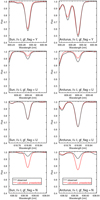 |
Fig. 1 Comparison of observed and calculated line profiles around four of the preselected Fe I lines with different gf_flag assignments for the Sun (left) and Arcturus (right). Black lines: observations, red lines: calculations including preselected spectral lines only. All of these lines are flagged with Y with respect to their blending properties. We would like to point out that the gf_flag assignments were based purely on the type of the gf-value sources. Theperformance of the lines in syntheses of the Sun and Arcturus were not taken into account. These are shown here for illustrative purposes only. |
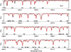 |
Fig. 2 Observed (black) and calculated (red) spectra for the Sun for an 8 nm-wide interval in the optical region. The Gaia-ESO bulk line list was used as input for the calculations, which includes preselected and background lines. Some of the strongest preselected lines are labelled by their species. |
Isotope information for the elements included in the preselected line list.
Isotopic splitting
For species with several stable isotopes of non-negligible abundances we provide transition data for each isotope separately, where available. For a given electronic state the different atomic masses of the isotopes result in different energy levels. Thus, a given transition can be regarded as split into several lines with different wavelengths for different isotopes. We would like to point out that the transition probabilities given for each isotopic component are the same. Accordingly, line list users need to scale the gf-values for isotopes by their relative abundances in the Solar System (Meija et al. 2016) for ‘normal’ stars, or as applicable for other isotopic compositions. The data used to calculate the isotopic splitting (IS) for the transitions under investigation are described and tabulated in Appendices B and C.
2.6 Other atomic data
So far we have discussed the atomic data needed to model the strengths of radiative transitions of the neutral and singly ionised atoms dominating the photospheres of FGK stars. However, to solve the radiative transfer problem and produce a synthetic spectrum a wealth of additional data are needed. These include data to describe the intrinsic widths and shapes of spectral lines (damping profile parameters), ionisation energies and partition functions to determine level populations under the assumption of local thermodynamic equilibrium, and continuous opacities. Most of these are provided as part of the Gaia-ESO line list together with the transition probabilities, and for others we refer to recent publications.
Natural or radiative broadening is caused by the limited life-times of the atomic states involved in the transitions. The width of the resulting damping profile is given by the sum of all transition rates for spontaneous deexcitations of both the upper level and the lower level. The radiative damping widths provided by R.L. Kurucz as part of his atomic structure calculations10 were included in the Gaia-ESO line list (via the VALD database). These data are available for many of the preselected lines. The exceptions are all of the Al I, Zn I, and Sr I lines, some of the Na I, Mg I, and Y II lines, and all lines for elements with Z > 40. For the lines without calculated radiative damping widths one can resort to using the classical description of a spectral line as a damped harmonic oscillator in a two-level atom11.
Further broadening of spectral lines is caused by elastic collisions between particles in the stellar atmosphere. Collisional broadening of hydrogen lines is addressed in Appendix B.1. Broadening of metal lines via the quadratic Stark effect due to impacting electrons and ions results in a damping profile which is parametrised by the Stark damping parameter. This effect is in general not very important in the atmospheres of FGK-type stars, as they contain few charged particles compared to the number of neutral particles (for exceptions see discussion in Barklem 2016, Sect. 4.1.2). For completeness, Stark broadening data were extracted from the VALD database and included in the Gaia-ESOline list, where available. In the same way as for radiative broadening, they come as a by-product of the calculations by R.L. Kurucz who computed them from sums over all possible transitions to a given level as describedin Kurucz (1981, p. 75). Collisional broadening by neutral hydrogen atoms is important for many metal lines, and is discussed in detail separately in Appendices E–H. In summary, collisional line widths for neutral and ionised Fe lines computed with the Anstee-Barklem-O’Mara (ABO) theory (Anstee & O’Mara 1991 and successive expansions by P.S. Barklem and collaborators) were compared to those computed by R.L. Kurucz and with the Unsöld recipe, which are based on Lindholm-Foley theory. The ratios between line widths from different theoretical approaches show a large spread, in particular for high values of the excitation energy. As the ABO theory is considered the most reliable theory (Barklem 2016), new broadening data were calculated according to the ABO theory for 41 lines of Fe I and eight other neutral species. These were included in the Gaia-ESO line list, together with previously available data for all other lines based on the ABO theory or provided by Kurucz, which had been extracted from the VALD database. Based on the analysis in Appendices E–H, we recommend avoiding lines of neutral species for which ABO data are not available (cf. Table 1). For lines of ionised species without ABO data that have low excitation energies, data by Kurucz should be used where available (Sc II, Ti II, and Y II lines), otherwise the Unsöldapproximation with an enhancement factor of 1.5 for the line width can be used (lines of rare-earth species).
For ionisation energies for atoms we refer to the NIST Atomic Spectra Database12 (Kramida et al. 2018), or Table 4 in Barklem & Collet (2016). Barklem & Collet (2016) calculated partition functions for all elements from H to U and the first three ionisation stages, for temperatures up to 10 000 K (their Table 8), based on excitation energies from the NIST ASD. Their data agree very well with those of Irwin (1987) for temperatures in common (i.e. above 1000 K) for most species. However, for some of the rare-earth elements, differences of up to 50% are seen (their Figs. 5 and 6). For La II the new partition functions are lower than Irwin (1987) at low temperatures, for Sm II and Eu II they are higher at low temperatures, and for Pr II and Dy II they are higher at high temperatures.
Finally, calculations of continuous fluxes are needed to be able to compare synthetic spectra to observations normalised to the continuum. This requires a large amount of input data for describing processes that are responsible for continuous opacities. These are bound-free and free-free transitions as well as scattering processes for numerous species which are abundant in cool stellar atmospheres. We did not define a standard set of data to be used for this aspect within GES. Instead, we refer to the data commonly used by the codes employed for Gaia-ESO data analysis. For example, the SME package and the MOOG code compute continuous opacities using adapted versions of the subroutines embedded in the ATLAS9 code by R.L. Kurucz13 (Kurucz 1970, p. 73). Obviously, the same routines are used in the SYNTHE code by Kurucz. For radiative transfer codes associated with the MARCS model atmosphere package (e.g. Turbospectrum) references for continuous opacity data are given in Table 1 of Gustafsson et al. (2008) and are discussed in their Sect. 4. For other codes see the references given in Smiljanic et al. (2014), who describe most of the Gaia-ESO analysis methods.
2.7 Blending properties for the sun and arcturus
In order to assess the blending properties of the preselected lines, two spectra each were calculated for parameters of the Sun and Arcturus (as described in Sect. 2.3). For one of the spectra we used only the preselected lines as input, and for the other one all the blending atomic and molecular lines from the background line list were included (Sects. 2.4 and 3).
The flags for blending properties (hereafter synflag) were assigned after visual inspection of the three overplotted line profiles (the two synthetic ones and the observed one) according to the following general scheme: Y indicates that the line is unblended or only blended with a line of the same species in both stars; U indicates that the line may be inappropriate in at least one of the stars; N indicates that the line is strongly blended with line(s) of different species in both stars. The number of lines to which the different synflag s were assigned for each species is indicated in Table 1.
Figure 4 shows typical example line profiles for four Fe I lines with accurate gf-values (gf_flag = Y) and with different synflag assignments. The top row shows the same line at 600.3 nm as the top row of Fig. 1. It is assessed to be unblended (synflag = Y), because all three spectra lie on top of each other. The second and third rows of Fig. 4 show examples for lines with undecided blending properties (synflag = U). The line at 522.5 nm has a weak blend at the red side in both stars and a possible additional unidentified blend as seen from the comparison with the observed Arcturus spectrum. The line at 540.1 nm is almost blend-free in the Sun but strongly blended in Arcturus. In addition, the data from the background line list around this line are incorrect, as is obvious from the comparison with the observed Arcturus spectrum. The bottom row of Fig. 4 shows an example for a line which is clearly blended in both stars (synflag = N).
We did not consider whether the strength of a line is appropriate for analysis in a specific star (i.e. not too weak or too strong), since this will vary much between survey targets. The blending assessment of a line should thus be valid only in comparison to other lines of the same species and line strength. This means for example that synflag = Y has been assigned to unblended lines in Arcturus even when they were not detectable in the Sun.
Observed line profiles for other benchmark stars with a wider range of stellar parameters are shown for the same four Fe I lines in Fig. 5 (see Sect. 2.3 for information on the spectra). For two stars of similar temperatureand gravity (e.g. dark brown dotted lines representing cool giants) the variation in line strength is due to the difference inmetallicity. The synflag = Y line seems blend-free in all stars (except the coolest dwarf star 61 Cyg A). The synflag = U and N lines are unblended in the warmer dwarfs and the metal-poor giant HD 122563, but they are blended in giant stars and cooler dwarfs. Further examples of Fe I lines with synflag = N are those at 516.6 and 517.2 nm, which lie on the wings of the Mg I b 516.7 and 517.3 nm lines. The line at 559.5 nm is a blend with a preselected Ca I line. Several further Fe I lines have weak blends in the Sun but strong blends in Arcturus (e.g. 547.3, 623.1 nm), and the reverse case is also encountered (e.g. 625.4, 635.9 nm). Examples for other species are given in Appendix B.
3 Molecular data
In addition to atomic data, we also include molecular data. In fact, the molecular transitions are much more numerous than the atomic transitions. Thus, it is crucial to include extensive molecular line lists for determining stellar parameters and identifying and fitting atomic line blends, although they also may be used for abundance determination and to derive isotopic ratios. Priority was given tomolecules which contribute significantly to the absorption in the spectra of G or K-type stars. This includes CH, NH, OH, C2, CN, MgH, SiH, CaH, FeH, TiO, VO, and ZrO (and their isotopologues). Although the best line lists available in the literature were used (Table 4)14, the quality of the molecular data varies from one molecule to the other.
For CH, NH, OH, and MgH, improved line lists were computed using high-quality laboratory line positions (better than 10−3 Å) combined with an accurate computation of transition moments (used to derive log gf for molecules). The laboratory line positions were used as input in the programme for simulating molecular spectra PGopher15 (Western 2017) in parallel with the programmes RKR1 and LEVEL16 (Le Roy 2017a,b) for derivation of the line intensities. Radiative broadening parameters were also computed whenever the information of the full electronic structure of the molecule was available. An illustration of the procedure for the case of CH can be found in Masseron et al. (2014). The line lists for the remaining molecules from the literature in general make use of the Born-Oppenheimer approximation to determine the positions and assume identical oscillator strengths for all isotopologues. In particular, the line lists for SiH, CaH, FeH, TiO, VO, and ZrO suffer from larger uncertainties, which for positions can sometimes reach several Å.
The molecular data are available at the CDS for the same wavelength ranges as the atomic data. The content of the CDS table is described in Sect. 4.3.
In addition to line positions and oscillator strengths, dissociation energies (Table 4) and partition functions are required to compute the molecular equilibrium. The partition functions used in this work are given in Table A.2.
Recently, Barklem & Collet (2016) reviewed partition functions and dissociation energies for a large number of diatomic molecules. Regarding dissociation energies, our selected values agree within 1% with the selection of Barklem & Collet (2016), except for CaH. However, because this molecule only appears in the coolest stars, this discrepancy should only have a marginal impact on the Gaia-ESO analysis. Concerning partition functions, an agreement better than 10% for temperatures lower than 5000 K is found between our adopted values and the compilation of Barklem & Collet (2016), except for FeH. We note that this latter molecule contributes only in the HR21 setting of the GIRAFFE instrument and only for very cool stars.
4 Discussion and outlook
4.1 Selected examples for the application of the line list
The Gaia-ESO line list has been used within the consortium for the determination of atmospheric parameters and abundances of calibration stars, stars across Galactic populations, and stars in several clusters. The results have been presented in over 50 refereed articles. Other spectroscopic surveys have also started to use the Gaia-ESO line list as a basis for their analyses. Examples for these are the EMBLA (Howes et al. 2016), GALAH (De Silva et al. 2015), and OCCASO (Casamiquela et al. 2016)surveys. Here, we briefly mention some of these works.
The Gaia FGK benchmark stars consist of about 30 well-known stars and were the main calibrators in the GES (Pancino et al. 2017). Reference values for metallicity (Jofré et al. 2014; Hawkins et al. 2016) and abundances of ten α- and iron-peak elements (Jofré et al. 2015) were determined from an analysis of high-resolution spectra. These works used a subset of the GES line list, where line selection was based on the quality flags17 and on low method-to-method dispersion. The standard deviations of the abundances of the Fe I lines derived by six different methods for each star were between 0.01 and 0.03 dex. The abundances of the remaining elements were derived by eight different methods differentially (line-by-line) to different reference stars after grouping the stars by atmospheric parameters. The decrease in dispersion for the differential line abundances compared to the absolute abundances confirmed, among other things, the importance of hyperfine structure effects. For each element, lines commonly used for stars within groups of similar spectral types were identified and were referred to as ‘golden lines’. In the case of Fe lines these were lines used for all stars within a group, and for the other elements a line was defined to be a golden line when it was analysed in at least 50% of the stars in the group. These include of the order of 100 Fe I lines, as well as the Si I line at 568.448 nm, which was used for all stars except two, to give some examples. For V and Co no golden lines were identified in metal-poor stars. A detailed discussion of golden lines can be found in Jofré et al. (2014, Sect. 6.3, Tables 4 and 5) and Jofré et al. (2015, Sect. 4.5 and online table18).
For the analysis of the UVES and GIRAFFE spectra observed within GES the different groups either used their own radiative transfer codes or a pre-computed grid of synthetic spectra. In both cases the Gaia-ESO line list was adopted. The grid contains 13 784 high-resolution synthetic spectra for FGKM-type stars over the spectral ranges 420–690 and 845–895 nm. A wide range of metallicities (from [M/H] = − 5.0 to +1.0 dex) and [α/Fe] enrichments (five values for each metallicity) is covered. For details see de Laverny et al. (2012). An overview of the analysis procedure of UVES spectra observed within the GES is given in Smiljanic et al. (2014) for the case of FGK stars in the field and in older open clusters, and by Lanzafame et al. (2015) for the case of F- to M-type stars in the fields of young open clusters with ages of less than 100 Myr. Atmospheric parameters (mainly based on Fe lines) and abundances of up to 24 or 26 elements were derived by up to 13 and four different groups, respectively. Their results were subsequently combined into a homogeneous set of recommended values. The groups made their individual choices of line sub-sets to be used with their methods. For an illustration of the variation in line selection for Ca I see Fig. 4 in Jofré et al. (2019). In the first case, spectral lines measured by at least three groups were included in the combined abundances, and lines affected by blends as indicated by synflag were removed for species with 20 lines or more. In the second case, one of the groups based their selection on synflag for elements with Z > 28, while the homogenisation was done without any further line selection. The precision of the abundances as indicated by the method-to-method dispersions was found to be similar in both cases, ranging from below 0.15 to 0.35 dex depending on the element. Stellar parameters and abundances of up to 11 chemical species were derived from GIRAFFE spectra observed within the GES by five different groups (A. Recio-Blanco, priv. comm., see also Worley et al. 2020). In this case the variation in line selection between groups is expected to be small because the number of lines in the relevant spectral range is low. Typical method-to-method dispersions in the combined and homogenised abundances were 0.04 dex.
Examples for studies of the structure and evolution of the Galactic bulge and disc based on the Gaia-ESO recommended metallicities and abundances are given in Williams et al. (2016), Bergemann et al. (2014), Recio-Blanco et al. (2014), and Mikolaitis et al. (2014). Typical mean uncertainties in abundances reported in these works are around 0.1 dex, which reflect the adoption of the Gaia-ESO line list, among other things. The abundance data allowed the authors to clearly distinguish between different sub-components in terms of metallicity and α-element abundances, and to derive trends of abundances with other stellar properties such as age or galactocentric radius. Lind et al. (2015) identified one star among a few hundred halo stars that has most likely been ejected from a globular cluster, based on a difference in [Mg/Fe] abundance of 0.8 dex at a 4σ significance compared to typical halo stars.
An example for advances in the area of open clusters made possible by GES spectra and the Gaia-ESO line list is given by three inner-disc clusters with ages of 0.3–1.5 Gyr. C, N, and O abundances with a typical precision of 0.05 dex were determined by Tautvaišienė et al. (2015), and abundances of 11 elements with average uncertainties of about 0.1 dex were determined by Magrini et al. (2015). In these works predictions made by models for stellar evolution and for Galactic chemical evolution were confirmed, and one cluster was found to be locally enriched by the Type II supernova explosion of a single star.
The EMBLA survey – an investigation of metal-poor stars in the Galactic bulge – is based on spectra obtained with a different instrument19, with similar resolution as the GES but covering a larger wavelength region (Howes et al. 2016). For the abundance analysis, the Gaia-ESO preselected line list was used as a starting point and was complemented by lines and data from other sources. There was a large overlap in line data between the two surveys for Fe II (mostly lines with gf_flag = Y), resulting in an average standard error of Fe line abundances of 0.06 dex. Other species with lines in common or with the same source for the gf-values were Ca I, Sc II, and Zn I, with mean uncertainties in abundances of ~0.1 dex, and Cr I and Ba II with ~0.2 dex. Carbonabundances were determined from CH band heads using the same molecular data as the GES, with uncertainties of ~0.2 dex. These data allowed the authors to conclude that the fraction of carbon-enhanced stars might be lower in the bulge compared to the halo, and that some of the other elements behaved differently in the bulge stars than in halo stars.
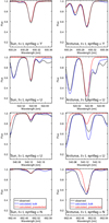 |
Fig. 4 Comparison of observed and calculated line profiles around four of the preselected Fe I lines with different synflag assignments for the Sun (left) and Arcturus (right). Black lines: observations, red lines: calculations including preselected spectral lines only, blue lines: calculations using the Gaia-ESO bulk line list, including preselected and background lines. All of these lines have gf_flag = Y. |
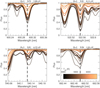 |
Fig. 5 Line profiles for four preselected Fe I lines generated from observed spectra of selected Gaia FGK benchmark stars (see Sect. 2.3). Quality flags and lower level energy are given at the top of each panel. The vertical dashed line indicates central wavelength. We note that Teff is coded by colour, solid lines are dwarfs, and dotted lines are giants. |
Molecular species, recommended dissociation energies D00, and references for molecular transitions.
4.2 Dataneeds and recent developments
This article describes version 6 of the Gaia-ESO line list, which was the last version produced within the GES consortium (mainly in 2014, with minor changes in 2016), and this is the version used for the final release of GES data products. The list is complete in the sense that it contains all atomic and molecular data available at the time of compilation for those transitions widely used for abundance analysis of FGK-type stars in the wavelength region of interest at the resolution of the FLAMES-UVES spectrograph. This includes hyperfine structure and isotope splitting data, as well as references to the original sources for the data. The list contains about 200 lines (not counting HFS or IS components) of 24 species which have accurate gf-values and are free of blends in the spectra of the Sun and Arcturus, that is, both gf_flag and synflag = Y (see column “Y/Y” in Table 1).
Prospective users of the line list are advised to update the gf-values with new data that may have become available since the compilation was done. Also, HFS and IS data are available for more species than considered relevant in the context of the GES, and users should add these according to the needs of their specific application. We note that for several species more recent calculations by R.L. Kurucz are available, in particular for C I, Si II, Ca I, Ti I, Ti II, V I, V II, Cr I, Cr II, Fe I (see discussion in Appendix B.16 for the latter). The Kurucz website provides HFS and IS components for many species.
Based on the presentation of available data in Appendix B we comment on those atomic species and lines for which future improvements of transition probability data should have the highest priority. We focus on the preselected lines with synflag = Y and U. A number of species have less than five such lines (see Table 1). Most of these have high-quality gf-values (gf_flag = Y), including the light species Li I, C I, O I, and Si II, and the heavy species Zn I, Zr II, Ru I, Ba II, Pr II, Sm II, Eu II, Gd II, and Dy II. The exceptions are V II, Sr I, and Y I which have one or two lines with theoretical gf-values. However, these lines are extremely weak and probably blended in most stellar spectra and thus of low priority for abundance analysis.
Among the species with at least five lines with synflag = Y or U several have high-quality gf-values for all of those lines (Sc I, Cu I, Y II, Zr I, Mo I) or for the vast majority (>90%, Ca I and Ti I). Another group of species has low-quality gf-values for more than 10%, but less than 50% of the synflag = Y or U lines (Sc II, Ti II, V I, Cr I, Mn I, Co I, La II, Ce II, Nd II). These should be considered for laboratory measurements in the long term, but they are of lower immediate priority. We note that for the five Sc II lines with gf_flag = N new theoretical gf-values based on branching fractions calculated using the relativistic Hartree–Fock method and life-times measured by Marsden et al. (1988) are available in Pehlivan Rhodin et al. (2017a). Finally, there are a number of species with low-quality gf-values for 50% or more of the synflag = Y or U lines, which should be given highest priority in current and future laboratory experiments.
The percentage is about 50 for both Fe I and Fe II. Specifically, 236 of 439 Fe I lines would need improved gf-values. These are roughly evenly distributed over the whole wavelength range considered here and comprise a wide variety of transitions. They originate from lower levels which are preferentially odd (70%) and belong to 36 different terms, of which the most frequent are y5 Fo and y3 Fo with energies of ~4.25 and ~4.60 eV, respectively. The upper levels are more diverse with 75 different terms, of which the most frequent are g5 F and f5 G with energies around 6.6 eV. One third of these lines have synflag = Y. Almost half of them have theoretical gf-values by Kurucz (2007, which should be replaced by more recent calculations available at the Kurucz website), and most of the remaining ones have gf-values measured by May et al. (1974). In the case of Fe II 13 of 26 lines have purely theoretical gf-values. These are listed in Table A.3 and half of them have synflag = Y.
About 60 to 70% of the synflag = Y or U lines need improved gf-values for the species Na I, Mg I, Si I, Ca II, and Ni I. These lines are also listed in Table A.3 except for Mg I and Ni I. For Mg I new experimental oscillator strengths were recently published by Pehlivan Rhodin et al. (2017b), combining branching fractions measured from an FTS spectrum of a hollow cathode discharge lamp with radiative life-times from the literature and from their own calculations. They also published new theoretical oscillator strengths based on the multiconfiguration Hartree-Fock method. All but one of the eight Mg I lines in the Gaia-ESO line list needing improvement are included in this work, as well as the four lines which already had high-quality gf-values. Table A.4 lists both the data in the GES line list and the new data for all of these lines.
Numerous Ni I lines found over the whole wavelength range considered here are candidates for new experimental transition probabilities (53 of 83 with synflag = Y or U). These lines are listed in Table A.5. Almost all of them currently have theoretical gf-values by Kurucz (2008). Nearly all of them originate from odd lower levels, which belong to 16 different terms, the most frequent one being y3 Fo with energies of ~4.2 eV. The upper levels belong to 14 different terms, the most frequent one being ![Mathematical equation: $3\textrm{d}^9(^2D_{5/2})4\textrm{d} \enspace^2[{{}^{7}}\!/\!{{}_{2}}]$](/articles/aa/full_html/2021/01/aa36291-19/aa36291-19-eq1.png) with energies around 6.1 eV. About 40% of these lines have synflag = Y.
with energies around 6.1 eV. About 40% of these lines have synflag = Y.
For Al I, S I, and Cr II none of the preselected lines with synflag = Y or U have high-quality gf-values (except for one Cr II line at 524.68 nm). Experimental work on these species is highly needed, and the 21 lines concerned are listed in Table 5.
Lines of Al I, S I, and Cr II with synflag = Y or U, and with gf_flag = U or N.
4.3 Access to data
The data comprising the Gaia-ESO line list in the wavelength ranges from 4750 to 6850 Å and from 8488 to 8950 Å are made available at the CDS. The atomic data are stored in a single table with one record for each transition. Hyperfine structure components and different isotopes are included as separate transitions, where applicable (see Sect. 2.5). HFS components belonging to the same fine structure transition can be identified by having the exact same label and J value for both the lower and the upper levels. Both the preselected lines and the background line list are included. Preselected lines can be identified byhaving both non-empty gf_flag and synflag entries. Here we describe the contents of the data fields included for each transition.
-
Element Element symbol (e.g. Fe).
-
Ion Ionisation stage (1 = neutral, 2 = singly ionised, 3 = doubly ionised).
-
Isotope Isotope information for Element: 0 if only one isotope is present in the list, otherwise the baryon number is given.
-
lambda Wavelength of the transition in air, in units of Å.
-
r_lambda Reference code for lambda.
-
loggf Logarithm (base 10) of the product of the oscillator strength of the transition and the statistical weight of the lower level.
-
e_loggf Uncertainty in loggf for experimental gf-values if available.
-
r_loggf Reference code for loggf. This field may contain several labels combined with + or |. When the labels are combined with + then loggf is the average from more than one source, while | means that relative gf-values from the first source were re-normalised to an absolute scale using accurate life-time measurements from the second source (see the respective subsection on Si, Ti, Fe, Cu, and Zn in Appendix B).
-
gf_flag Flag indicating the relative quality for loggf (usage recommendation, values Y/U/N, see Sect. 2.2), for preselected lines only.
-
synflag Flag indicating the blending quality of the spectral line for synthesis (usage recommendation based on spectra of the Sun and Arcturus, values Y/U/N, see Sect. 2.7), for preselected lines only.
-
Label_low A string of characters specifying the electronic configuration and the term designation for the lower energy level. Taken from the VALD database, which follows the notation adopted by the NIST Atomic Spectra Database20.
-
J_low Total angular momentum quantum number J for the lower level.
-
E_low Lower level energy in units of eV.
-
r_E_low Reference code for E_low.
-
Label_up Configuration and term label for the upper energy level.
-
J_up Total angular momentum quantum number J for the upper level.
-
E_up Upper level energy in units of eV.
-
r_E_up Reference code for E_up.
-
Rad_damp Logarithm of the radiative damping width in units of rad s−1 (see Sect. 2.6).
-
r_Rad_damp Reference code for Rad_damp.
-
Sta_damp Logarithm of the Stark broadening width per unit perturber number density at 10 000 K, in units of rad s−1 cm3 (see Sect. 2.6).
-
r_Sta_damp Reference code for Sta_damp.
-
Vdw_damp Van der Waals broadening parameter (see Sect. 2.6 and Appendices E–H). Values greater than zero were obtained from ABO theory and are expressed in a packed notation where the integer component is the broadening cross-section, σ, in atomic units, and the decimal component is the dimensionless velocity parameter, α. Values less than zero are the logarithm of the broadening width per unit perturber number density at 10 000 K in units of rad s−1 cm3.
-
r_Vdw_damp Reference code for Vdw_damp.
The atomic data are available in their entirety in a machine-readable form at the CDS. Table 6 lists excerpted data fields from the CDS data table containing all the atomic line parameters, for guidance regarding the content of the CDS table. When the values for the fields e_loggf, Rad_damp, Sta_damp, and Vdw_damp are equal to zero, this means that they are not available for the respective transition. Field names starting with r_ contain reference codes, that is, labels to be used with the provided BibTeX file (see below). Table 6 does not contain the fields Label_low and Label_up, which are however present for each line in the CDS table. As a single example, the strings given in fields Label_low and Label_up for the C I line listed in Table 6 are ’LS 2s2.2p.3p 1P’ and ’LS 2s2.2p.4d 1P*’, respectively (where multiple white spaces were collapsed into one).
The molecular data are stored in similar form, with two data fields for both element symbol and isotope information (Element_1, Element_2, Isotope_1, Isotope_2), a subset of the remaining data fields (lambda, loggf, E_low, E_up, Rad_damp), and the following additional data fields:
-
State_low Lower level electronic state symbol.
-
State_up Upper level electronic state symbol.
-
v_low Lower level vibrational quantum number.
-
v_up Upper level vibrational quantum number.
-
Branch Label indicating branch – a string of characters in most cases consisting of the branch designation (e.g. P, Q, R), the spin components (1, 2,...), the rotationless parity (e or f) whenever lambda doubling has been computed, and in parentheses the total angular momentum quantum number (J) for the lower level. For further explanations we refer to the references for the sources of molecular data (see Table 4).
-
r_mol Reference code.
We would like to point out that the quantum numbers were not used for the calculation of synthetic spectra within the GES. The data are available in their entirety in a machine-readable form at the CDS. An excerpt is shown in Table 7 for guidance regarding the content of the CDS table.
We strongly encourage users of the Gaia-ESO line list to cite, in addition to this overview article, the individual sources for the atomic and molecular data used in a particular work. It is important that providers of atomic data receive credit for their work by citing the original publications. This is also a prerequisite for the continued funding of this type of research. To facilitate citations of original sources we provide, together with the data tables, a BibTeX file with the relevant entries.
Examples for atomic data.
Examples for molecular data.
Acknowledgements
We are thankful for the contributions of Enrico Maiorca, Matthew P. Ruffoni, and Jennifer Sobeck to the line list work. We thank Robert L. Kurucz for information on his calculations. U.H. and A.J.K. acknowledge support from the Swedish National Space Agency (SNSA/Rymdstyrelsen). K.L. acknowledges funds from the European Research Council (ERC) under the European Union’s Horizon 2020 research and innovation programme (Grant agreement No. 852977). Š.M. acknowledges support from the Research Council of Lithuania (LMT) through grant LAT-08/2016. T.M. acknowledges support from the State Research Agency (AEI) of the Spanish Ministry of Science, Innovation and Universities (MCIU) and the European Regional Development Fund (FEDER) under grant AYA2017-88254-P. J.C.P. acknowledges support from the STFC of the UK. T.B. and U.H. were supported by the project grant “The New Milky Way”from the Knut and Alice Wallenberg Foundation. A.R.C. is supported in part by the Australian Research Council through a Discovery Early Career Researcher Award (DE190100656). Parts of this research were supported by the Australian Research Council Centre of Excellence for All Sky Astrophysics in 3 Dimensions (ASTRO 3D), through project number CE170100013. P.J. acknowledges funds from FONDECYT Iniciación Grant number 11170174. R.S. acknowledges support from NCN through grant 2014/15/B/ST9/03981 and from the Polish Ministry of Science and Higher Education. This work has made use of the VALD database, operated at Uppsala University, the Institute of Astronomy RAS in Moscow, and the University of Vienna. Based on data products from observationsmade with ESO Telescopes at the La Silla Paranal Observatory under programme ID 188.B-3002. These data products have been processed by the Cambridge Astronomy Survey Unit (CASU) at the Institute of Astronomy, University of Cambridge, and by the FLAMES/UVES reduction team at INAF/Osservatorio Astrofisico di Arcetri. These data have been obtained from the Gaia-ESO Survey Data Archive, prepared and hosted by the Wide Field Astronomy Unit, Institute for Astronomy, University of Edinburgh, which is funded by the UK Science and Technology Facilities Council. This work was partly supported by the European Union FP7 programme through ERC grant number 320360 and by the Leverhulme Trust through grant RPG-2012-541. We acknowledge the support from INAF and Ministero dell’ Istruzione, dell’ Università’ e della Ricerca (MIUR) in the form of the grant “Premiale VLT 2012”. The results presented here benefit from discussions held during the Gaia-ESO workshops and conferences supported by the ESF (European Science Foundation) through the GREAT Research Network Programme.
Appendix A Auxiliary tables
This appendix provides five tables with auxiliary data referred to in Sects. 2.1, 3, and 4.2.
Transitions for which multiple fine-structure components were merged into one line in the preselected line list.
Polynomial coefficients for partition functions (Q) for molecules.
Lines of Fe II, Na I, Si I, and Ca II with synflag = Y or U, and with gf_flag = U or N.
Atomic data for Mg I lines with synflag = Y or U.
Ni I lines with synflag = Y or U, and with gf_flag = U or N.
Appendix B Detailed description of atomic data
We discuss the data sources and quality aspects for the lines of each atomic species element by element. For each element included in the preselected line list the sources for transition probabilities (oscillator strengths) and the assignment of the quality flag for gf-values (gf_flag) are discussed. This is supplemented by a discussion of the blending properties and the assignment of the corresponding quality flag (synflag). Finally, if applicable, the sources for HFS and IS data are presented. Sources for the gf-values of elements appearing only in the background line list are summarised in Appendix D.
The following species are included in the preselected line list (see Table 1 for an overview): H I, Li I, C I, O I, Na I, Mg I, Al I, Si I, Si II, S I, Ca I, Ca II, Sc I, Sc II, Ti I, Ti II, V I, V II, Cr I, Cr II, Mn I, Fe I, Fe II, Co I, Ni I, Cu I, Zn I, Sr I, Y I, Y II, Zr I, Zr II, Nb I, Mo I, Ru I, Ba II, La II, Ce II, Pr II, Nd II, Sm II, Eu II, Gd II, Dy II.
B.1 Hydrogen (Z = 1)
Hydrogen being the simplest of atoms, the transition probabilities can be calculated from first principles (e.g. Gray 2005, p. 236). The source for the hydrogen Balmer and Paschen lines used here is Wiese & Fuhr (2009, gf_flag = Y). An extended list for Paschen lines, including highly excited transitions from principal quantum numbers >20 can be found in Kurucz (1993)21.
Broadening of hydrogen lines due to the presence of electrons and ions via the linear Stark effect needs to be taken into account, using for example the refined calculations by Stehlé & Hutcheon (1999), which however in practise are quite similar to the seminal work by Vidal et al. (1973). An accurate description of resonance broadening of H lines due to collisions with other hydrogen atoms (self-broadening) is given in Barklem et al. (2000a), which has further been improved by Allard et al. (2008) for the case of the Hα 656.2 nm line. A recent review on hydrogen Balmer lines can be found in Barklem (2016, Sect. 4.1.1), and a ready-to-use implementation is made available by P. Barklem and N. Piskunov22.
B.2 Lithium (Z = 3)
The gf-values for the two Li I 670.8 nm resonance fine structure transitions were taken from the theoretical calculation of Yan et al. (1998). These are essentially identical to the theoretical values quoted in Yan & Drake (1995) and Wiese & Fuhr (2009). The predicted life-time of the 2p 2P° upper level of these transitions from these calculations agrees extremely well with the experimental measurements of Volz & Schmoranzer (1996) and McAlexander et al. (1996). The transition probabilities are considered accurate (gf_flag = Y).
We adopted the highly accurate isotopic splitting data of Sansonetti et al. (1995) from frequency-modulation spectroscopy, which are in excellent agreement with the Fourier-transform spectrometry measurements of Radziemski et al. (1995). The latter authors also report HFS constants from the literature. However, HFS components were not computed for the Gaia-ESO line list. The transition probabilities for the Li I 610.3 nm subordinate lines in the background line list come from Lindgård & Nielson (1977).
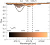 |
Fig. B.1 Observed spectra of selected Gaia FGK benchmark stars around the Li I 670.8 nm feature (see Sect. 2.3). |
The Li I 670.8 nm feature is often weak and blended to varying degrees in different stars (synflag = U, see Fig. B.1). Lithium abundances are therefore best derived using spectral synthesis. Unfortunately, the available atomic data in the region around the Li I feature are quite poor. They cannot be used directly for abundance determination and require an astrophysical calibration. This concerns in particular two Fe I and two V I lines located within 0.4 Å from the Li I feature. The two lines bluewards of Li I are by far too weak in a synthetic spectrum of the Sun and Arcturus, while the two lines redwards of Li I are by far too strong, when using the gf-values from Kurucz (2007, 2008) for Fe I and V I, respectively.
In order to provide a good basis for the Gaia-ESO analysis the following changes were made (log gf-Kurucz → log gf-GES): Fe I 670.743 nm, − 3.917 →−2.2; V I 670.752 nm, − 2.938 →−0.8; V I 670.809 nm, − 2.443 →−2.75; Fe I 670.828 nm, − 1.280 →−2.85. The Fe I 670.743 nm is one of the preselected lines (quality N/U), while the remaining lines are part of the background line list. These modifications result in a much improved synthesis for the Sun and Arcturus in this region (see Fig. B.2).
B.3 Carbon (Z = 6)
For three permitted and one forbidden C I lines in the preselected line list, we adopted the theoretical transition probabilities of Hibbert et al. (1993). We used the Length values rather than the Velocity values as recommended by the authors, which are in good agreement with those calculated as part of the Opacity Project (Luo & Pradhan 1989) when assuming LS coupling. Unfortunately, no recent accurate experimental measurements exist for these transitions but the theoretical values are considered reliable (gf_flag = Y). For the [C I] 872.7 nm line the here adopted log gf value by Hibbert et al. (1993) is 0.03 dex larger than the recommended value by Wiese & Fuhr (2007), which stems from the calculations of Tachiev & Froese Fischer (2001). The transition probabilities for the other C I lines in the background line list come from Kurucz (2010b), and from NIST (Ralchenko et al. 2010), which are almost exclusively based on Hibbert et al. (1993) and Luo & Pradhan (1989). The four C I lines primarily used for abundance purposes are typically weak and partly blended (synflag = U) except for the 658.7 nm line which is considered largely clean (synflag = Y). Considering the low natural abundance of the 13 C isotope (see Table 3) neither isotopic nor HFS components were included.
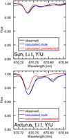 |
Fig. B.2 Line profiles around the Li I feature for the Sun and Arcturus. Black lines: observations, red lines: calculations including preselected spectral lines only, blue lines: calculations including blends from background line list. For Arcturus the Li abundance was set to log (εLi) +12 = −0.8 dex, where εLi = NLi∕NH (e.g. Brown et al. 1989; Guiglion et al. 2016). |
B.4 Oxygen (Z = 8)
For the [O I ] 557.7 nm forbidden line the predictions from Baluja & Zeippen (1988), Galavis et al. (1997) and Froese Fischer & Tachiev (2012) agree well. They can furthermore be put on an accurate absolute scale using the life-time measurement of the 2p1 S upper level by Corney & Williams (1972) to yield loggf(557.7) = −8.241. For the O I 615.8 nm line we adopted the transition probability from Hibbert et al. (1991) assuming LS coupling. The adopted gf-values for the [O I ]630.0 and 636.4 nm forbidden lines are the mean of the theoretical predictions of Storey & Zeippen (2000) and Froese Fischer & Tachiev (2012): loggf(630.3) = −9.715 and loggf(636.3) = −10.190. All four theoretical transition probabilities are considered reliable (gf_flag = Y). For the other O I lines in the background line list the transition probabilities were adopted from the NIST database (Ralchenko et al. 2010), which are largely based on Hibbert et al. (1991) and the Opacity Project (Butler & Zeippen 1991) assuming LS coupling.
As discussed for example in Asplund et al. (2009), all of the four preselected O I lines are partly blended (synflag = U with synflag = N for the case of 557.7 nm). In particular, the Ni I 630.0342 nm line in the background line list is very close to the [O I ] line at 630.0304 nm, and its gf-value of − 2.11 was explicitly taken from Johansson et al. (2003) to replace the value of − 2.674 from Kurucz (2008) contained in the VALD database.
B.5 Sodium (Z = 11)
Accurate (gf_flag = Y) experimental transition probabilities exist for the Na I 589 nm doublet from Volz et al. (1996). In the absence of reliable experimental data for the other preselected Na I lines we adopted the theoretical gf-values from Froese Fischer & Tachiev (2012), which have been classified as gf_flag = U. The data for other Na I lines in the background line list come from the NIST database (Ralchenko et al. 2010). Besides the Na I D lines the following three Na I lines are considered largely clean (synflag = Y): 568.8, 615.4 and 616.0 nm.
Sodium is exclusively in the form of 23Na with a nuclear spin of 3/2. Sodium is thus prone to hyperfine splitting which however has not been accounted for in the Gaia-ESO line list. Suitable HFS data are available in Das & Natarajan (2008), including the Na I D lines at 589 nm.
B.6 Magnesium (Z = 12)
The gf-values for optical Mg I lines are notoriously uncertain with few experimental data to rely on until recently (see discussion of new data by Pehlivan Rhodin et al. 2017b in Sect. 4.2). An exception is found for the Mg I b triplet lines, which have accurate transition probabilities provided by Aldenius et al. (2007) from measurements of life-times and branching fractions (BFs). For the other Mg I lines in the preselected line list we adopted theoretical values from Froese Fischer & Tachiev (2012, line at 880.7 nm, gf_flag = Y), from the Opacity Project (Butler et al. 1993) under the assumption of LS coupling, or from Chang & Tang (1990), the latter two with gf_flag = U. Several of these lines are considered largely clean (synflag = Y). For Mg I lines only appearing in the background line list we rely on values given by Ralchenko et al. (2010) if available and otherwise by Kurucz & Peytremann (1975). Isotopic splitting or HFS components are not measurable in Mg I spectra of natural isotopic composition (Pehlivan Rhodin et al. 2017b).
B.7 Aluminium (Z = 13)
No reliable experimental data exist for the Al I lines in the Gaia-ESO line list. We therefore resorted to using the theoretical calculations by the Opacity Project (Mendoza et al. 1995) under the assumption of LS coupling with a gf_flag = U rating for the five Al I lines in the preselected line list. The same gf-values were adopted by Scott et al. (2015a) in their recent analysis of the solar chemical composition. Of the available Al I lines, only 669.867 nm is considered largely unblended (synflag = Y). For other Al I lines in the background line list we make use of Kurucz (1975, unpublished) and Wiese et al. (1969). Aluminium consists entirely of 27 Al, which has nuclear spin 5/2. While not accounted for explicitly in the Gaia-ESO line list, good HFS data are available in for example Nakai et al. (2007) and Sur et al. (2005), see Nordlander & Lind (2017, their Table A.2).
B.8 Silicon (Z = 14)
When available, we adopted the experimental transition probabilities of Garz (1973) for Si I, which are however only reliable in a relative sense. Therefore we re-normalised them to an improved absolute scale in the same manner as Scott et al. (2015a) with the highly accurate, laser-induced fluorescence (LIF) life-times of the 4s 3 P0,1,2 levels measured by O’Brian & Lawler (1991), resulting in a gf_flag = Y rating. For a few Si I lines not available in Garz (1973), we rely on the Opacity Project calculations of Nahar (1993), which were obtained under the close-coupling approximation with the R-matrix method (gf_flag = U). These data were complemented by the extensive calculations of Kurucz (2007, gf_flag = N) for a considerable number of lines.
For the two Si II lines at 634.711 and 637.137 nm in the preselected line list we adopted the same gf-values as in Scott et al. (2015a), which were obtained from taking the mean of Schulz-Gulde (1969), Blanco et al. (1995), and Matheron et al. (2001) and are given a gf_flag = Y evaluation. For Si I lines only appearing in the background line list we made use of Kurucz (2007).
There are three Si I lines with a simultaneous gf_flag = Y and synflag = Y rating, at 569.043, 570.110 and 594.854 nm, while the remainder of the Garz (1973) lines in the preselected line list are partly blended. A comparison of line abundances derived for four benchmark stars (see Sect. 2.3) for two different sets of lines (with gf_flag = Y and gf_flag = N) can be seen in Fig. B.3, while mean abundances are given in Table B.1. The gf_flag = N lines generally result in a larger scatter of line abundances than the gf_flag = Y lines, although the statistical significance is low owing to the small number of gf_flag = Y lines.
B.9 Sulphur (Z = 16)
For the S I triplets at 674.3 and 674.8 nm and the lines at 675.7 and 869.4 nm only theoretical gf-values are available. We adopted the mean transition probabilities of Froese Fischer & Tachiev (2012) and Zatsarinny & Bartschat (2006), which are given a gf_flag = U rating. All of these are also partly blended (synflag = U). The gf-values for other S I lines in the background line list mainly come from the theoretical calculations by Biemont et al. (1993) and Kurucz (2004).
B.10 Calcium (Z = 20)
Highly accurate experimental gf-values are availablefor most of the preselected Ca I lines (gf_flag = Y). The majority of these have been determined by Smith & Raggett (1981). Others have been published by Smith (1988), Drozdowski et al. (1997), and Aldenius et al. (2009). We also included a few lines without experimental gf-values, for which we used the calculations by Froese Fischer & Tachiev (2012) with gf_flag = U. About one third of these lines are largely blend-free in the Sun and Arcturus (synflag = Y, see Table 1). Two examples are illustrated in Fig. B.4. The line at 526.039 nm was used for most of the FGK dwarfs and giants in the abundance determination for benchmark stars by Jofré et al. (2015), and the line at 649.965 nm for most of the FG dwarfs and the metal-poor stars in the same study (see also Sect. 4.1).
For Ca II only few experimental gf-values exist. We instead rely on theoretical data from the Opacity Project (Saraph & Storey 2012, gf_flag = U) under the assumption of LS coupling, as discussed in detail in Mashonkina et al. (2007), and on calculations by Theodosiou (1989) for the NIR triplet lines (gf_flag = Y). For two of the NIR triplet lines the calculations by Theodosiou (1989) show excellent agreement with the experimental data by Gallagher (1967). We note that the values of Theodosiou (1989) are approximately 0.05 dex higher than those from Saraph & Storey (2012), which were included in version 4 of the Gaia-ESO line list. Figure B.5 shows the solar observed and synthetic spectrum (see Sect. 2.3) for the NIR triplet lines, which are the most important Ca II lines in the GIRAFFE setting used by the GES. The pressure sensitivity of the lines provides an excellent gravity constraint for dwarf stars, in particular the lines at 854.2 and 866.2 nm (synflag = Y). All other preselected Ca II lines are blended to some degree (synflag = U or N).
Data for Ca I lines in the background line list were also taken from Smith (1981) and Kurucz (2007), in addition to the references above. For Ca II lines we used additional data from Seaton et al. (1994) and Kurucz (1999). The three Ca I autoionising lines at 631.811, 634.331, and 636.175 nm lie within the Gaia-ESO wavelength range and are included in the background line list. To enable a realistic modelling of their Fano profiles the radiative damping parameters were assigned values derived from the Shore parameters provided by R.L. Kurucz23. The first Shore parameter is the radiative width (Shore 1967), which is given in frequency units by Kurucz as log10(Γf), where Γf is the full width at half maximum (FWHM) in Hz. The radiative damping parameter in the Gaia-ESO line list (and in the Kurucz lists for lines other than autoionising lines) is log10(Γ), where Γ is the FWHM in angular frequency units (rad s−1). Thus, to convert to the usual radiative damping parameter, one uses Γ = 2πΓf, and thus log10(Γ) = log10(Γf) + 0.80, and this value is given in the line list.
The remaining two parameters given by Kurucz are the Shore parameters a and b describing the profile shape. The three lines have an asymmetry parameter a of practically zero (log10(a) = −30 cm2g−1), which implies a Lorentz absorption profile with no asymmetry (i.e. the equivalent Fano parameter q = ∞; see Shore 1967). Thus, an appropriate radiative damping parameter achieves the same result as the profile according to the Shore parameterisation of the Fano profile. Tests indicate that these data reproduce profiles in standard stars reasonably well. The presence of the autoionising lines affects the derivation of abundances from other lines that fall in this region, an example being Zn (see Appendix B.20).
B.11 Scandium (Z = 21)
For both Sc I and Sc II lines the gf-values of Lawler & Dakin (1989) are to be preferred (gf_flag = Y, including all of the preselected Sc I lines). These authors determined BFs using emission FTS measurements, while the absolute scale was obtained using the time-resolved laser-induced fluorescence (TRLIF) life-times of Marsden et al. (1988). For a few preselected Sc II lines without experimental gf-values we used the calculations by Kurucz (2009, gf_flag = N). The background line list also contains gf-values from Martin et al. (1988).
Only the two Sc I lines at 535.6 and 621.1 nm and the two Sc II lines with high-quality gf-values at 565.8 and 566.7 nm are blend-free (synflag = Y). Examples for Sc II line profiles are shown in Fig. B.6. The line at 565.790 nm was used for most of the FGK dwarfs and the metal-poor stars in the abundance determination for benchmark stars by Jofré et al. (2015), and the line at 660.460 nm for most of the FGK dwarfs and giants (see also Sect. 4.1).
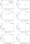 |
Fig. B.3 Line-by-line Si I abundances determined for four benchmark stars for two groups of lines with different quality assessment of their transition probabilities, as a function of equivalent width and lower level energy. Abundances are given as log (εSi) + 12, where εSi = NSi∕NH. Only lines with synflag = Y or U and with equivalent widths >5 mÅ are included. |
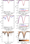 |
Fig. B.4 Observed and calculated line profiles around two preselected Ca I lines for the Sun (top row) and Arcturus (middle row). Black lines: observations, red lines: calculations including preselected spectral lines only, blue lines: calculations including blends from background line list. Bottom row: line profiles generated from observed spectra of selected Gaia FGK benchmark stars. See Sect. 2.3. |
HFS data
For Sc I a wealth of HFS data from both experimental and theoretical studies are available. Childs (1971) employed the atomic-beam magnetic-resonance technique (ABMR) resulting in highly accurate data for the  levels. ABMR data were also presented by Ertmer & Hofer (1976) and Zeiske et al. (1976) for the
  levels, which we employ. For several others, including the
  levels, the only source of data are the calculations published by Başar et al. (2004). The high-excitation levels are represented by the theoretical predictions by Öztürk et al. (2007). The complete set of HFS data is given in Table C.1. For Sc II no HFS components were computed, but HFS data for most of the preselected Sc II lines can be found in Scott et al. (2015b, their Sect. 6.1.2 and Table 2).
B.12 Titanium (Z = 22)
For Ti I we adopted transition probabilities primarily from Nitz et al. (1998) and Lawler et al. (2013), and for Ti II we preferred Wood et al. (2013). Nitz et al. (1998) measured BFs for Ti I from FTS spectra and combined those with accurate TRLIF life-times from Salih & Lawler (1990), and Lawler et al. (2013) expanded on that work. In addition, we used accurate gf-values from Grevesse et al. (1989), produced by re-normalising the relative oscillator strengths from the Oxford group (Blackwell et al. 1982a, 1983, 1986) with the absolute scale fixed by using the TRLIF life-times of Rudolph & Helbig (1982). We also used data by Smith & Kuehne (1978) for one line. All lines with data from these sources were assigned a gf_flag of Y. For the remaining few Ti I lines we used the semi-empirical calculations by Kurucz (2010b, gf_flag = N).
Abundance statistics (number of lines, mean, and standard deviation of log εX + 12, where εX = NX∕NH) for four species and four Gaia FGK benchmark stars.
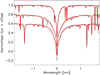 |
Fig. B.5 Observed (black dotted lines) and synthesised (red solid lines) solar spectra of the Ca II near-infrared (NIR) triplet linesat 849.8, 854.2, and 866.2 nm, from top to bottom. The lines are shifted with respect to their central wavelength and offsets are added to the normalised fluxes for clarity. |
Most of the Ti II lines in the preselected line list are covered by the high-quality FTS and echelle work by Wood et al. (2013). Another FTS study by Pickering et al. (2001) produced gf-values for many lines but relied on calculated oscillator strengths of weak lines to complete the fractions for some branches. To put their BFs on an absolute scale Pickering et al. (2001) used life-times from Bizzarri et al. (1993) or life-times derived from the theoretical transition probabilities of Kurucz (2010b). These data were used for two of the lines. All lines from these two sources were assigned a gf_flag of Y, while the data for the remaining few Ti II lines were taken from Kurucz (2010b) with gf_flag = N.
The Ti I lines are the second most numerous (after Fe I) among the preselected lines (see Table 1), and 90% of them have high-quality gf-values. Among those, 24% are also unblended in the Sun and Arcturus (synflag = Y). In contrast, there is only one among the 18 Ti II lines with gf_flag = Y which also is blend-free (541.877 nm). Examples for line profiles are shown in Fig. B.7. The Ti I line at 597.854 nm was used for most of the FGK dwarfs and giants in the abundance determination for benchmark stars by Jofré et al. (2015), and the Ti II line at 487.401 nm for most of the FG dwarfs, the FGK giants, and the metal-poor stars in the same study (see also Sect. 4.1).
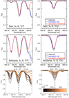 |
Fig. B.6 Observed and calculated line profiles around two preselected Sc II lines for the Sun (top row) and Arcturus (middle row). Black lines: observations, red lines: calculations including preselected spectral lines only, blue lines: calculations including blends from background line list. Bottom row: line profiles generated from observed spectra of selected Gaia FGK benchmark stars. See Sect. 2.3. |
The background line list relies mainly on calculations by Kurucz (2010b), and for Ti I on data from Martin et al. (1988), Nitz et al. (1998), and Lawler et al. (2013). For a few Ti II lines in the background line list experimental data and astrophysical determinations were used (Ryabchikova et al. 1994; Pickering et al. 2001; Wood et al. 2013).
Titanium has five isotopes with non-negligible natural abundances (see Table 3), including two with non-zero spin. Isotopic splittings are presented in Scott et al. (2015b, their Sect. 6.2.2 and Table 2) for two and six of the preselected Ti I and Ti II lines, respectively, together with HFS constants. The largest wavelength shifts between two isotopes are 0.04 Å for Ti I, and <0.03 Å for Ti II. None of the lines have HFS data for both levels. Therefore, neither isotopic nor HFS components were included in the Gaia-ESO line list for Ti.
B.13 Vanadium (Z = 23)
The work ofWhaling et al. (1985) provides the most accurate measurements of V I oscillator strengths to date, based on both FTS BFs and TRLIF life-times. Most of our preselected V I lines are covered by this source (gf_flag = Y), and about 40% of these lines are also unblended in the Sun and Arcturus (synflag = Y). Line profiles for the V I line at 611.952 nm are shown in Fig. B.8 (left column) as a representative example. This line was used for the largest number of FGK dwarfs and giants in the determination of the V abundance for benchmark stars by Jofré et al. (2015) (see also Sect. 4.1).
For 13 out of the 49 preselected V I lines and most of the lines in the background line list, the gf-values come from the calculations of Kurucz (2009, gf_flag = N), except when data are available in Martin et al. (1988). For V II all gf-values come from the calculations of Kurucz (2010b, gf_flag = N), including the three preselected lines.
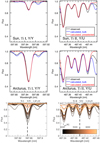 |
Fig. B.7 Observed and calculated line profiles around two preselected Ti I and Ti II lines for the Sun (top row) and Arcturus (middle row). Black lines: observations, red lines: calculations including preselected spectral lines only, blue lines: calculations including blends from background line list. Bottom row: line profiles generated from observed spectra of selected Gaia FGK benchmark stars. See Sect. 2.3. |
HFS data
A large number of good experimental data on the HFS of V I is available, with only few levels being included in more than one study. We followed the quality assessment of Scott et al. (2015b), who sorted the data into three groups of published works with no overlap between works within each group. Data were then selected according to order of preference. The group with the most preferred data comprises the studies of Childs et al. (1979, ABMR and LFS – laser fluorescence spectroscopy – data), El-Kashef &Ludwig (1992, ABMR), and Unkel et al. (1989, ABMR). The second-best group consists of measurements by Palmeri et al. (1995, FTS), Lefèbvre et al. (2002, FTS), and Cochrane et al. (1998, crossed beam). Data for levels not in the previous two groups were taken from Unkel et al. (1989, LFS). The complete set of HFS data is given in Table C.2.
B.14 Chromium (Z = 24)
Sobeck et al. (2007) measured highly accurate Cr I oscillator strengths using FTS BFs normalised to TRLIF life-times of Cooper et al. (1997). Together with the data from Blackwell et al. (1984) for one line these were assigned the gf_flag = Y. These data were complemented with experimental transition probabilities from Martin et al. (1988), Cocke et al. (1973), and Wolnik et al. (1968), and with semi-empirical gf-values from Kurucz (2010b), although with gf_flag = N.
Among the 35 lines with high-quality gf-values there are nine which also are blend-free in the Sun and Arcturus (synflag = Y), and a further 15 lines with uncertain blend status (synflag = U). Line abundances derived for four benchmark stars (see Sect. 2.3) for these lines are compared to line abundances for gf_flag = N lines in Fig. B.9, while mean abundances are given in Table B.1. For the Sun and Arcturus the scatter of the gf_flag = N lines is twice as large as the scatter of the gf_flag = Y lines, while it is comparable for the cool dwarf star 61 Cyg A, for which all of the lines might be blended to some degree.
For a few of the preselected Cr II lines experimental oscillator strengths were taken from Pinnington et al. (1993, gf_flag = Y). For the remaining lines we used the semi-empirical oscillator strengths from Kurucz (2010b, gf_flag = N). More than half of the Cr II lines are heavily blended in the Sun and Arcturus (synflag = N), and among the remaining ones there is only one with synflag = Y (530.585 nm), which unfortunately does not have an experimental gf-value (see also Sect. 4.2). In the background line list the majority of the Cr II gf-values come from Raassen & Uylings (1998), supplemented by data from Sigut & Landstreet (1990), Martin et al. (1988), and the two sources above.
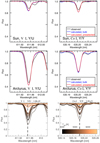 |
Fig. B.8 Observed and calculated line profiles around preselected lines of V I (left) and Co I (right) for the Sun (top) and Arcturus (middle). Black lines: observations, red lines: calculations including preselected spectral lines only, blue lines: calculations including blends from background line list. Bottom: line profiles generated from observed spectra of selected Gaia FGK benchmark stars. See Sect. 2.3. |
Chromium has four isotopes with non-negligible natural abundances (see Table 3), including one with non-zero spin. Isotopic splitting and HFS data for Cr are scarce and are given for one Cr I line in Scott et al. (2015b, their Sect. 6.4.2 and Table 2), which is not among our preselected lines. The wavelength difference between the lightest and heaviest Cr isotope is just 0.003 Å and can be ignored in the context of the GES.
B.15 Manganese (Z = 25)
For Mn I lines we used accurate experimental gf-values from Den Hartog et al. (2011) and Blackwell-Whitehead & Bergemann (2007). For some lines data were taken from Booth et al. (1984). See Scott et al. (2015b) for a more detailed discussion of these sources. They cover about three quarters of the preselected lines, and all of them were assigned a gf_flag = Y. For the remaining preselected Mn I lines we resorted to the calculations of Kurucz (2007, gf_flag = N). In addition, the background line list contains Mn I data from Martin et al. (1988) and Blackwell-Whitehead et al. (2005a), and Mn II lines with calculated gf-values from Kurucz (2009).
We note that for three Mn I lines (601.349, 601.664, 602.179 nm) the upper level energy values in Den Hartog et al. (2011) are incorrect in the fifth digit, leading to a shift in wavelength of 0.02 to 0.03 Å (see Jofré et al. 2017). The wavelengths adopted in the line list are therefore taken from Kurucz (2007).
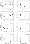 |
Fig. B.9 Line-by-line Cr I abundances determined for four benchmark stars for two groups of lines with different quality assessment of their transition probabilities, as a function of equivalent width and lower level energy. Abundances are given as log (εCr) + 12, where εCr = NCr∕NH. Only lines with synflag = Y or U and with equivalent widths >5 mÅ are included. |
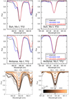 |
Fig. B.10 Observed and calculated line profiles around two preselected Mn I lines for the Sun (top row) and Arcturus (middle row). Black lines: observations, red lines: calculations including preselected spectral lines only, blue lines: calculations including blends from background line list. Bottom row: line profiles generated from observed spectra of selected Gaia FGK benchmark stars. See Sect. 2.3. |
Only three of the Mn I lines with high-quality gf-values have synflag = Y (542.035, 539.467, 602.179 nm), but a further 15 may be useful for abundance analysis if a careful evaluation of blending lines is done (synflag = U). Two of these lines are shown in Fig. B.10. The line at 482.352 nm was used for most of the metal-poor stars in the abundance determination for benchmark stars by Jofré et al. (2015), and the line at 601.349 nm for most of the FGK dwarfs and giants in the same study (see also Sect. 4.1).
HFS data
For the HFS data we again followed the quality assessment of Scott et al. (2015b) and selected accurate experimental data from several groups of publications, in the following order of preference: (1) Davis et al. (1971, spin-exchange), Johann et al. (1981, ABMR), Dembczyński et al. (1979, ABMR), and Brodzinski et al. (1987, interference spectroscopy); (2) Başar et al. (2003, optogalvanic spectroscopy) for the z4 D level, Blackwell-Whitehead et al. (2005b, FTS) for all other levels; (3) Lefèbvre et al. (2003, FTS), Luc & Gerstenkorn (1972, FTS and Fabry-Perot spectrometry), and Handrich et al. (1969). The complete set of HFS data is given in Table C.3.
B.16 Iron (Z =26)
The first choice for the source of gf-values for Fe I lines are the publications by three laboratory spectroscopy groups from the 1980s and 1990s. The groups are those based in Oxford, UK (Blackwell et al. 1979a,b, 1982b,c, 1986), Madison, Wisconsin (O’Brian et al. 1991), and Hannover, Germany (Bard et al. 1991; Bard & Kock 1994). The Oxford group used absorption spectroscopy to determine very precise relative gf-values, which were put on an absolute scale using one line with an accurate (± 0.02 dex) transition probability. The high-quality Madison and Hannover gf-values are based on emission spectroscopy, which provided life-times and BFs.
For the Madison dataset the gf-values were calculated from the original published data (vacuum wavenumber  in cm−1, transition probability Aul in s−1, and upper level rotational quantum number Jupp), using the following equation:
 (B.1)
(B.1)
where me, c, and e are the electron mass, the speed of light, and the electron charge, respectively, all in SI units (see e.g. Gray 2005).
Recently, Ruffoni et al. (2014) and Den Hartog et al. (2014) used a similar technique to determine transition probabilities for 142 and 203 Fe I lines, respectively, about 70 and 60 of which fall in the main Gaia-ESO wavelength regions (UVES-580 and GIRAFFE HR21 settings), and 35 and 37 of which are among the preselected lines. They focused on lines with high values of lower level energy, 3− 6 eV, with few measurements reported by the above mentioned groups.
For lines in common between all of the above sources the log gf-values were averaged, using weights based on the experimental uncertainties. In total, we obtained data from these sources for 45% of the 545 Fe I lines in the preselected line list, and assigned the gf_flag Y to them.
For lines not present in any of the above sources gf-values from May et al. (1974) were used if available (28% of the preselected lines). These were assigned the gf_flag U, except for ten high-excitation lines with small uncertainties (0.05 dex or less), which are also unblended (synflag Y or U, gf_flag = Y). We stress here that we elected to adopt the original values of May et al. (1974) rather than those subsequently re-normalised by Fuhr et al. (1988) based on more recent life-time measurements. This choice was made after realising that in the wavelength region covered by the GES data the original gf-values agree significantly better with our four preferred sources for lines in common, as illustrated in Fig. B.11.
For a few lines we used older laboratory data from Garz & Kock (1969), Richter & Wulff (1970), and Wolnik et al. (1970, 1971), choosing this time to trust the re-normalisation by Fuhr et al. (1988). We have not rigorously investigated the performance of original and re-normalised data in this case, but assigned gf_flag U in all cases. The same ranking wasmade for four lines from Bridges & Kornblith (1974) and Kock et al. (1984) with absolute values re-normalised by Fuhr & Wiese (2006). For the remaining 25% of the preselected lines we used the semi-empirical calculations from Kurucz (2007, gf_flag = N). Figure B.12 illustrates how well lines with different gf_flag s perform with respect to each other in an abundance analysis. Line abundances derived for four benchmark stars (see Sect. 2.3) for 240–290 Fe I lines with synflag Y or U and equivalent widths > 5 mÅ are shown, while mean abundances for lines with equivalent widths ≤100 mÅ are given in Table B.1. A significant increase in scatter can be seen for lines with the poorest ranking, which supports our recommendations. Abundances for lines with gf_flag = N deviate from the mean by up to 2 dex. However, also among gf_flag = U and Y lines with small quoted laboratory uncertainties there are individual exceptions with poor astrophysical performance. Examples are the gf_flag = Y lines at 506.008 nm (0.0 eV, synflag = U, equivalent widths of 68, 174, 16, 117 mÅ in the Sun, Arcturus, HD 22879, and 61 Cyg A, respectively) and at 522.318 nm (3.635 eV, synflag = Y, equivalent widths of 28, 56, 6, and 38 mÅ in the four stars), which result in ~0.5 dex higher24 and lower abundances than other gf_flag = Y lines with similar equivalent widths, respectively.
 |
Fig. B.11 Comparison of Fe I transition probabilities published by May et al. (1974) to newer, more accurate data from the Oxford, Madison, Hannover, and London groups (see text for references). The solid line indicates the proposed normalisation of the May et al. (1974) values by Fuhr et al. (1988). Applying this normalisation would shift the zero-point on the vertical axis to the solid line (while the data points would remain at the same positions relative to the solid line). All published spectral lines in the wavelength region 476 to 895 nm are shown. |
The most accurate Fe II gf-values come from the compilation of Meléndez & Barbuy (2009). Their data are based on relative gf-values within each multiplet taken from theoretical works, and a calibration using experimental life-times (Hannaford et al. 1992; Schnabel et al. 1999, 2004) and BFs (e.g. Kroll & Kock 1987; Heise & Kock 1990). Solar calibrated values from Meléndez & Barbuy (2009) were not considered here. This source is the preferred choice and was used for 19 preselected lines, for which the gf_flag was set to Y. For the remaining 23 preselected lines the gf-values were taken from the theoretical work of Raassen & Uylings (1998), and the gf_flag was set to U.
In the background line list the majority of the Fe I gf-values are based on the semi-empirical calculations by Kurucz (2007). They are supplemented by data from May et al. (1974) and Fuhr et al. (1988), as well as the Oxford, Madison, Hannover, and London groups. We assigned a gf_flag = Y to 148 Fe I lines in the background line list, which have data from the latter, ‘first choice’ gf-value sources (while the synflag is not defined for any of these lines). We used theoretical data from Kurucz (2013) for about one third of the Fe II gf-values, in addition to the data from Raassen & Uylings (1998).
The overall situation of transition probabilities for Fe lines was investigated by Lind et al. (2017, their Sect. 2.2.2 and Fig. 4). They compared semi-empirical calculations made available by R.L. Kurucz in 2014 with available experimental data for about 2000 Fe I lines (out of more than 500 000 possible radiative bound-bound transitions) and found differences of up to ±1 dex for transitions with loggf ≳−2, which increased to − 3 dex for transitions with loggf ~−4 and high upper level energies. The compilation of the line list presented here was completed shortly before the new calculations by Kurucz for Fe I became available, which is the reason why the previous calculations from 2007 were adopted. A comparison of the Kurucz data from 2007 with experimental data results in a figure which is very similar to Fig. 4 of Lind et al. (2017), with only a few more deviating points appearing at loggf ≲−5. A direct comparison of the 2007 data with the 2014 data shows that the gf-values have changed by more than 0.5 dex for only about 50 out of 2000 lines.
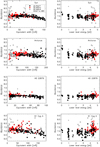 |
Fig. B.12 Line-by-line Fe I abundances determined for four benchmark stars for three groups of lines with different quality assessment of their transition probabilities, as a function of equivalent width and lower level energy. Abundances are given as log (εFe) + 12, where εFe = NFe∕NH. Only lines with synflag = Y or U and with equivalent widths >5 mÅ are included. |
We note that any line list is prone to being incomplete, as only about half of the lines visible in high-quality solar spectra have identified counterparts with good wavelengths according to Kurucz (2014). Many of these lines are expected to stem from iron, as indicated in the recent works by Peterson & Kurucz (2015) and Peterson et al. (2017), who present Fe I lines newly identified from an analysis of carefully selected stellar spectra. About 1200 of these lines fall in the wavelength range considered here, and for about 20% of them the authors provide astrophysically-determined gf-values. While the nature of the GES speaks against the usage of astrophysical gf-values, as explained in Sect. 2.2, these data should be included in future line lists of other projects, potentially providing for more realistic synthetic spectra.
B.17 Cobalt (Z = 27)
The most recent accurate Co I oscillator strengths were determined by Nitz et al. (1999) from FTS BFs put on an absolute scale using their own TRLIF life-time measurements (Nitz et al. 1995). Reliable data are also available from Cardon et al. (1982). These are the gf_flag = Y sources used for 70% of the preselected Co I lines, supplemented by calculations of Kurucz (2008, gf_flag = N). The overall quality status for preselected Co I lines is similar to that of Cr I with eight synflag = Y lines among those with high-quality gf-values, and a further 14 lines with synflag = U (see Table 1). Line profiles for the Co I line at 535.204 nm are shown in Fig. B.8 (right column) as a representative example. This line was used for the largest number of FGK dwarfs and giants in the determination of the Co abundance for benchmark stars by Jofré et al. (2015) (see also Sect. 4.1). In addition, the background line list contains Co I data from Martin et al. (1988) and Lawler et al. (1990), and Co II lines with calculated gf-values from Raassen et al. (1998) and Kurucz (2006).
HFS data
For Co I HFS we used the data measured by Pickering (1996), who used more than 1000 line profiles acquired with the high-resolution FTS at Imperial College. This yielded HFS A and B constants for 297 energy levels, comprising almost all known Co I energy levels (Pickering 1996). The complete set of HFS data is given in Table C.4.
B.18 Nickel (Z= 28)
Our preferred Ni I oscillator strengths come from the recent work by Wood et al. (2014), who measured FTS and echelle spectrograph BFs and used the TRLIF life-times of Bergeson & Lawler (1993) to provide the absolute scale. Thesewere available for 31 preselected Ni I lines. For the Ni I line at 481.198 nm the high-quality gf-value from Johansson et al. (2003) was used, which was derived from FTS BFs and a single TRLIF life-time. For the line at 542.465 nm the gf-value was taken from Doerr & Kock (1985). Data from the above sources were assigned the gf_flag Y. For four lines we used somewhat older experimental data from Lennard et al. (1975, gf_flag = U). For the remaining 62 preselected lines we resorted to calculations by Kurucz (2008, gf_flag = N). About one third of the latter are blend-free in the Sun and Arcturus (synflag = Y), and one half have uncertain blend status (synflag = U). These lines should be given high priority for new laboratory measurements of gf-values (see Sect. 4.2). However, Ni abundances may be determined with confidence from the currently available data, as about half of the lines with high-quality gf-values also have synflag = Y, and the other half has synflag = U (see Table 1).
Line abundances derived for four benchmark stars (see Sect. 2.3) for Ni I lines with synflag Y or U and equivalent widths >5 mÅ are shown in Fig. B.13, while mean abundances for lines with equivalent widths ≤ 100 mÅ are given in Table B.1. For the Sun and Arcturus the scatter around the mean value is similar for the gf_flag = Y and gf_flag = N lines, but the N lines result in a systematically lower mean abundance by ~0.1 dex than the Y lines. We note, however, that all the N lines are high-excitation lines (Elow ~ 4 eV), while most of the Y lines are low-excitation lines (Elow ≲ 2 eV). Therefore, the abundance difference may be related to modelling deficiencies rather than atomic data issues. For HD 22879 and 61 Cyg A the mean abundances of the different sets of lines are more similar, but the N lines show a twice as large scatter than the Y lines.
Nickel consists of five stable isotopes, dominated by 58 Ni and 60 Ni in the Solar System (see Table 3). The single isotope with non-zero spin contributes only 1% to the natural Ni abundance, and thus HFS can be ignored. Isotopic components were not included in the Gaia-ESO line list but are listed for eight lines in Table 2 of Scott et al. (2015b, see also their Sect. 6.8.2). Five of these lines are among our preselected lines, including three lines with both gf_flag and synflag = Y (617.681, 622.398, and 637.825 nm). The largest wavelength shift including all isotopes is 0.05 Å, while the shifts for the dominating isotopes are ≲0.03 Å. The background line list contains Ni I data from Fuhr et al. (1988) and Wickliffe & Lawler (1997a), in addition to the sources above, as well as Ni II data from Kurucz (2003).
B.19 Copper (Z = 29)
For the six preselected Cu I lines we adopted the experimental gf-values from Kock & Richter (1968). To be fully consistent with Grevesse et al. (2015) we re-normalised these to the improved life-times of Carlsson et al. (1989), although in terms of gf-values the change is less than 0.01 dex. The transition probabilities of these Cu I lines are rated as accurate (gf_flag = Y). One of the six Cu I lines is considered largely clean (578.213 nm, synflag = Y) for abundance purposes, while the others are blended to varying degrees (synflag = U). For Cu I lines only appearing in the background line list we adopted transition probabilities from Kurucz (2012), as well as from Biémont (1973) for a few lines. In the Solar System Cu consists to more than two thirds of 63 Cu and almost one third 65Cu, both of which have non-zero nuclear spin and therefore cause hyperfine splitting (see Table 3). Table C.5 provides the adopted data for HFS and isotope shifts.
B.20 Zinc (Z = 30)
For the two preselected Zn I lines at 481.053 and 636.234 nm the gf-values were taken from the theoretical work of Biemont & Godefroid (1980). In the case of 481.053 nm this was further slightly re-normalised to the more accurate life-times measured by Kerkhoff et al. (1980) as in Grevesse et al. (2015). These transition probabilities are rated reliable (gf_flag = Y), but the lines are partly blended (synflag = U), including 636.234 nm which is located in a Ca I autoionising line. The isotopes 64 Zn, 66 Zn, and 68 Zn all contribute significantly to the Solar System abundance of Zn (see Table 3), but data for isotopic shifts are not available. Hyperfine splitting is of little importance owing to the low natural abundance of the single isotope of Zn with non-zero spin.
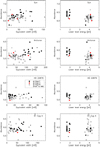 |
Fig. B.13 Line-by-line Ni I abundances determined for four benchmark stars for three groups of lines with different quality assessment of their transition probabilities, as a function of equivalent width and lower level energy. Abundances are given as log (εNi) + 12, where εNi = NNi∕NH. Only lines with synflag = Y or U and with equivalent widths >5 mÅ are included. |
B.21 Strontium (Z = 38)
Oscillator strengths for the preselected Sr I lines were taken from García & Campos (1988) with gf_flag = Y (five lines), Werij et al. (1992) and Vaeck et al. (1988) with gf_flag = U, and Corliss & Bozman (1962) with gf_flag = N. García & Campos (1988) measured relative transition probabilities from emission-line spectrometry in a hollow cathode discharge lamp. These were placed on an absolute scale using previously published experimental life-times by other authors. The data from Werij et al. (1992) are derived from a combination of R-matrix multichannel-quantum-defect-theory and modified Coulomb-approximation calculations, complemented by branching-ratio measurements.
None of the preselected lines are blend-free in the Sun or Arcturus, and there are only two lines with synflag = U (679.102 nm with gf_flag = Y and 654.678 nm with gf_flag = U). Both of these are very weak, and the remaining eight Sr I lines have synflag = N. The background line list also contains a few Sr II lines, with data from Warner (1968).
Strontium has three stable isotopes, one of them with non-zero spin (see Table 3). Owing to the low Solar System abundance of the latter, we expect the effect of HFS to be negligible for Sr. Hughes (1957) presented measurements of isotope shifts for 13 Sr I lines within the Gaia-ESO wavelength range. All of them have negligible shifts (≲2 mÅ).
B.22 Yttrium (Z = 39)
For the few Y I lines in the preselected line list only the semi-empirical calculations by Kurucz (2006) are available, which were adopted for this work. Because the accuracy of these values is not known they were assigned a gf_flag = N. All of these lines are furthermore blended to some degree in the Sun and Arcturus (see Table 1).
The situation is much better for the more numerous Y II lines, all of which are contained in the recent experimental work by Biémont et al. (2011) and were assigned a gf_flag = Y. Four of these lines are also unblended in the Sun and Arcturus (synflag = Y; 488.368, 508.742, 528.982, 572.889 nm), and seven additional lines have uncertain blend status (synflag = U). The background line list also contains data from Kurucz (2011) for Y II.
Yttrium has only one stable isotope, which has non-zero spin (see Table 3). HFS data are listed in Table 2 of Grevesse et al. (2015, see also their Sect. 4.8) for seven of our preselected Y II lines. However, these data result in HFS components with negligible wavelength difference (≲5 mÅ).
B.23 Zirconium (Z = 40)
For the preselected Zr I lines we adopted the gf-values of Biemont et al. (1981), who measured life-times and branching ratios by laser-induced fluorescence and emission spectrometry. For two of the three preselected Zr II lines we used the experimental transition probabilities of Ljung et al. (2006, gf_flag = Y), and for the third line the estimated oscillator strength of Cowley & Corliss (1983, gf_flag = U) was used. In addition to these sources the background line list contains Zr I data from Corliss & Bozman (1962) and oscillator strengths estimated by R. L. Kurucz from multiplet table intensities for Zr I and Zr II lines.
The Zr lines are all very weak in solar-type stars but can be quite strong in cooler stars. Two examples are shown in Fig. B.14. Thus, a detailed blending analysis and line selection should be done whenever stars are analysed whose parameters differ from those of the Sun and Arcturus. Five of the Zr I lines seem to be good candidates for abundance analysis and were assigned synflag = Y, with the remainder having synflag = U. The three Zr II lines all seem to be affected by blends (see Table 1).
Zirconium has five stable isotopes which all contribute significantly to the Solar System abundance (see Table 3). Three of them contribute at the 20% level or more, and all of these have zero spin. Therefore we did not include any HFS components25. Isotopic shifts were measured by Langlois & Gagné (1994) for 330 Zr I lines between 536 and 706 nm. The maximum shift between 90 Zr and 94 Zr in their list was 8 mÅ. Similar values have been reported by Bourauel et al. (1987) and Lim et al. (1998). This level of isotopic splitting is negligible in the context of the GES.
B.24 Niobium (Z = 41)
Accurate experimental oscillator strengths for the eight preselected Nb I lines were measured by Duquette et al. (1986). In addition, the background line list contains Nb I data from older measurements of Corliss & Bozman (1962) and Duquette & Lawler (1982). Niobium has one isotope with a nuclear spin of 9/2 and can therefore be expected to show hyperfine structure. Because the Nb lines are all weak, HFS splitting has not been accounted for, but relevant data can be found in Nilsson & Ivarsson (2008) and Nilsson et al. (2010). All of the Nb I lines are heavily blended (synflag = N).
B.25 Molybdenum (Z = 42)
Experimental transition probabilities for the six preselected Mo I lines are available from Whaling & Brault (1988), who used measured radiative life-times and branching ratios. These are rated accurate (gf_flag = Y). The Mo lines are all very weak, and therefore hyperfine and isotope splitting have not been accounted for. The primary Mo abundance indicators are 575.141 and 603.064 nm (synflag = Y), although they are too weak in dwarfs to be useful (see Fig. B.15).
B.26 Ruthenium (Z = 44)
We included one line of Ru I in the preselected line list (486.9 nm) with an experimental (life-time and branching ratio) gf-value from Wickliffe et al. (1994). The line is not included in the more recent work of Fivet et al. (2009). The adopted gf-value is considered accurate (gf_flag = Y), but the line is significantly blended (synflag = U). In addition, the background line list contains Ru I data from Corliss & Bozman (1962), Biemont et al. (1984), Salih & Lawler (1985), and R. L. Kurucz (based on multiplet tables). The Ru lines are all very weak and therefore hyperfine and isotope splitting have not been accounted for.
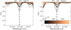 |
Fig. B.14 Line profiles for two high-quality preselected Zr I lines, which are weak in solar-type stars but strong in cooler stars. Generated from observed spectra of selected Gaia FGK benchmark stars. See Sect. 2.3. |
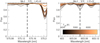 |
Fig. B.15 Line profiles for high-quality preselected Mo I lines generated from observed spectra of selected Gaia FGK benchmark stars. See Sect. 2.3. |
B.27 Barium (Z = 56)
We used the experimental data from Davidson et al. (1992) for all four preselected Ba II lines. Two of the lines are also included in the experimental work of Kurz et al. (2008). The loggf values from Kurz et al. (2008) are lower than those from Davidson et al. (1992) by ~0.1 dex. For consistency, we adopted the source containing all four lines. All four lines are strong in stellar spectra except for the most metal-poor stars. The line at 493.408 nm is strongly blended in all but the most metal-poor stars (see Fig. B.16). In addition, the background line list contains Ba I data from Corliss & Bozman (1962) and data from Miles & Wiese (1969) for Ba I and Ba II lines.
HFS and IS data
Solar System material contains a mixture of several stable Ba isotopes, five of which contribute with more than 1% to the Ba abundance (Table 3). Isotopic splittings have been measured for the 493.408 nm line by Wendt et al. (1984), for the 585.367 and 614.171 nm lines by Van Hove et al. (1982), and for the 649.690 nm line by Villemoes et al. (1993). The wavelength shifts are summarised in a table in the online database of R.L. Kurucz26 and the largest ones are 2 mÅ (between isotopes 134 and 138). Although this can be considered to have a negligible effect in the context of the GES and similar surveys, all five isotopic components were included for the preselected Ba II lines.
Two of the isotopes have non-zero nuclear spin leading to HFS in Ba II lines with non-negligible effects on abundance analysis. Experimental determinations of the HFS A and B constants were found for all levels involved in the preselected Ba II lines in Becker et al. (1981), Silverans et al. (1986), and Villemoes et al. (1993). The complete set of HFS data is given in Table C.6.
B.28 Lanthanum (Z = 57)
We used experimental data from Lawler et al. (2001a) for five of the preselected La II lines (gf_flag = Y). For the sixth line at 593.6 nm the only experimental data available are from Corliss & Bozman (1962), which is known to have large, systematic uncertainties (see e.g. Arnesen et al. 1977; Wahlgren 2010). We did not attempt to apply any corrections to the Corliss & Bozman (1962) data or adopt any previous such attempts. Instead, we resorted to the theoretical value from Kułaga-Egger & Migdałek (2009). To assess the uncertainty inherent in that work we compared transition probabilities for lines in common with Lawler et al. (2001a), as shown in Fig. B.17. The comparison shows a similar scatter as the comparison between the Lawler et al. (2001a) data and data from Bord et al. (1996, see Figs. 1 to 3 in Lawler et al. 2001a), which are based on a semi-empirical calibration of data from Meggers et al. (1975). We assigned a gf_flag = U to the 593.6 nm line. In addition, the background line list contains data for La I and La II by Corliss & Bozman (1962) and for La II by Zhiguo et al. (1999).
Most of the preselected lines are blended to different degrees in the spectra of the Sun, Arcturus, and other benchmark stars (see Figs. B.18 and B.19). The line at 492.2 nm appears rather clean in observed spectra, but a synthesis including surrounding lines from the background line list yields a significantly stronger line than a synthesis for the La II line only. A look into the background line list reveals several lines of different species with similar strength at the same wavelength (Si I, Ti I, Ce II, Y I). Hence, the line is not recommended for abundance analysis (synflag = N). The only line with synflag = Y at 593.6 nm is invisible in spectra of dwarf stars and weak in spectra of giant stars but might be stronger in spectra of r-process-rich, metal-poor stars.
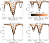 |
Fig. B.16 Line profiles for preselected Ba II lines generated from observed spectra of selected Gaia FGK benchmark stars. See Sect. 2.3. |
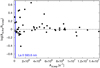 |
Fig. B.17 Comparison between theoretical (the) and experimental (exp) transition probabilities Aul for La II. Data are from Kułaga-Egger & Migdałek (2009) and Lawler et al. (2001a), respectively. The blue vertical line indicates the location of the line at 593.6 nm. |
HFS data
The single dominant isotope 139La makes up 99.9% of La in Solar System material (Table 3). Thus, La lines will not be affected by isotopic splitting.
On the other hand, HFS should be taken into account for the analysis of La lines. We extracted A and B constants from the literature for each of the nine energy levels involved in the preselected La II transitions, where possible. Most of the data were taken from the experimental work based on ion-beam-laser spectroscopy by Höhle et al. (1982). A similar type of measurement was found for one level in Li et al. (2001). For another two levels HFS constants measured from FTS spectra were found in Lawler et al. (2001a). Semi-empirical calculations of HFS data for the upper level of the line at 492.2 nm are provided in Furmann et al. (2008), but were not included in the line list. The complete set of HFS data is given in Table C.7.
B.29 Cerium (Z = 58)
High-quality experimental data for Ce II lines from BFs and life-times are available from Lawler et al. (2009, gf_flag = Y) for two thirds of the 12 preselected lines. For the other lines we used theoretical data from Palmeri et al. (2000, gf_flag = U). The latter used two different approaches to calculate radiative life-times, designated “Calculation A” and “Calculation B”. According to the authors, Calculation B is expected to be more accurate than Calculation A. Palmeri et al. (2000) give gf-values using Calculation B for selected lines, including one of the lines considered here (511.7 nm). The background line list contains numerous additional Ce II lines with data from these two sources, as well as Ce I lines with data from Corliss & Bozman (1962) and Cowley (1973).
The values for the three preselected NIR lines are taken from the online DREAM database27, which appears to provide the results of Calculation A of Palmeri et al. (2000). In addition to having uncertain gf-values, none of these three lines is recommended for abundance analysis due to their unfavourable blending properties (synflag = U or N).
Among the optical lines two appear unblended in the spectra of the Sun, Arcturus, and other benchmark stars (Fig. B.20, lower panels), while two others are strongly blended and cannot be recommended for abundance analysis (Fig. B.20, upper panels). The remaining lines were assigned a synflag = U, and their usage needs to be decided on a case-by-case basis.
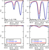 |
Fig. B.18 Comparison of observed and calculated line profiles around the two La II lines at 492.2 nm (upper panels, gf_flag = Y, synflag = N), and at 593.6 nm (lower panels, gf_flag = U, synflag = Y) for the Sun (left) and Arcturus (right). Black lines: observations, red lines: calculations including preselected spectral lines only, blue lines: calculations including blends from background line list. |
Cerium has four stable isotopes, all with zero nuclear spin. Two of them contribute to the Solar System abundance with more than 1% (Table 3). However, the isotope splitting is negligible for Ce II lines (Lawler et al. 2009)
B.30 Praseodymium (Z = 59)
Experimental gf-values are available for all seven preselected Pr II lines from Ivarsson et al. (2001, six lines) and from Li et al. (2007a, four lines), where three lines are in common. In general, the data from the two publications agree well (see Fig. 2 of Sneden et al. 2009). An exception is the line at 532.3 nm (0.2 dex difference in loggf). Sneden et al. (2009) found that the higher value from Li et al. (2007a) results in a more consistent solar Pr abundance. Synthetic spectra calculated for Arcturus with scaled solar abundances and the Li et al. (2007a) gf-value also supportthe validity of the higher value (see Fig. B.21). In summary, we used the data from Ivarsson et al. (2001) for five lines, and data from Li et al. (2007a) for two lines (521.7 nm and 532.3 nm), all with gf_flag = Y.
We note that the gf-values given in Table 2 of Li et al. (2007a) do not agree with the values obtained by using their Eq. (5), with differences reaching more than 0.005 dex in some cases. We used the calculated values instead of the tabulated ones (the differences calculated minus tabulated are +0.017 dex and −0.018 dex for the two lines, respectively). In addition to the sources above, the background line list contains Pr II data from Biémont et al. (2003), data from Meggers et al. (1975) for Pr I and Pr II lines, and data from Ryabtsev (priv. comm.) for a few Pr III lines.
Most of the preselected Pr II lines are invisible and/or severely blended in the spectra of the Sun, Arcturus, and other benchmark stars. However, two lines at 526.0 and 532.3 nm have non-negligible strengths and seem to be more or less unblended (synflag = U and Y, respectively, see Fig. B.21). Five of the lines (the previous two and 517.4, 522.0, 529.3 nm) were used by Sneden et al. (2009) to derive the Pr abundance in r-process-rich, metal-poor ([Fe/H] ≈ −3 dex) stars, in which these lines are stronger than in the Sun.
HFS data
Praseodymium has a single stable isotope, 141Pr, with non-zero nuclear spin, giving rise to HFS in Pr II lines. For each of the 12 energy levels involved in the preselected Pr II transitions HFS A constants are available in the literature. Electric quadrupole interaction is considered negligible for the HFS of Pr (e.g. Ginibre 1989; Sneden et al. 2009), and thus the HFS B constants were set to zero for all levels. Five of the levels are included in the experimental work based on fast-ion-beam laser spectroscopy by Rivest et al. (2002). Data for the remaining levels were taken from the work of Ginibre (1989), who determined HFS A constants from an analysis of FTS spectra. The complete set of HFS data is given in Table C.8.
B.31 Neodymium (Z = 60)
With over 50 lines Nd II lines are the most numerous among all rare earth species in the preselected line list. For the majority of these lines, including one of the four lines in the NIR, we used the experimental gf-values determined by Den Hartog et al. (2003, gf_flag = Y) from a combination of LIF measurements of radiative life-times and FTS measurements of BFs. The gf-values for the remaining lines (reference code MC in the CDS table) are from Kurucz & Bell (1995). They are derived from a calibration of measured line intensities from Meggers et al. (1975) following the procedure outlined by Cowley & Corliss (1983, T.A. Ryabchikova and R.L. Kurucz, priv. comm.). A comparison of the MC-derived data to the Den Hartog et al. (2003) data for 133 lines in common within the UVES-580 wavelength range is shown in Fig. B.22. The comparison is characterised by a standard deviation of 0.22 dex and additional systematic differences varying with wavelength. We assigned a gf_flag = U to the gf-values from this source.
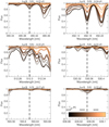 |
Fig. B.19 Line profiles for preselected La II lines generated from observed spectra of selected Gaia FGK benchmark stars. See Sect. 2.3. |
For five lines with MC-derived data there are also experimental gf-values by Li et al. (2007b) available (which are between 0.04 dex larger and 0.16 dex smaller), but these were not included in the line list. In addition, the background line list contains data from Meggers et al. (1975) for Nd I lines, from Xu et al. (2003a) for Nd II lines, and from Ryabchikova et al. (2006) for Nd III lines.
The four preselected Nd II lines in the NIR are invisible in solar-like and giant stars, with the possible exception of one line in metal-rich giants such as μ Leo. Only two of the lines in the UVES-580 range appear unblended in solar- or Arcturus-like stars (synflag = Y). However, their gf-values are uncertain, and at least one of them could be affected by unidentified blends. About half of the remaining lines are clearly blended (synflag = N), and the other half are border-line cases or lines for which the blending properties strongly depend on stellar parameters (synflag = U). A few selected cases are illustrated in Figs. B.23 and B.24. We note that this assessment is not directly applicable to r-process-rich, metal-poor stars, for which the relative strengths of Nd II lines and blending lines might be significantly different.
HFS and IS data
Neodymium has seven stable isotopes with rather evenly distributed Solar System abundance ratios (Table 3). Data for IS are available for all of the preselected Nd II lines for the isotope pair 144–150 and for 41 of the lines for the isotope pair 142–144. For the remaining isotopes the wavelengths were set to those of isotope 150. The shifts in level energy for the 142–144 pair were measured by Ahmad & Saksena (1981) on hollow cathode lamp spectra recorded by a Fabry-Perot spectrometer. For the 144–150 pair most of the required levels were measured by Nakhate et al. (1997) using the same technique. Complementary data for the remaining levels were taken from the extensive FTS work by Blaise et al. (1984). The complete set of IS data used in the Gaia-ESO line list is given in Table C.9.
Koczorowski et al. (2005) measured isotopic shifts for 27 levels of Nd II for all pairs of Nd isotopes with even baryon number, using the LIF method (including 13 of the lowest levels and eight of the upper levels of the preselected transitions). Their results are consistent with the sources cited above. The derived shift values are similar for all pairs, although the values for the 150–148 pair tend to be larger than for the others.
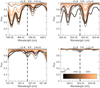 |
Fig. B.20 Line profiles for preselected Ce II lines generated from observed spectra of selected Gaia FGK benchmark stars. See Sect. 2.3. |
Two of the Nd isotopes have odd baryon numbers with non-zero spin and thus hyperfine structure. For 11 even-parity low-energy levels and 64 odd-parity high-energy levels of 143Nd HFS A and B constants were measured by Rosner et al. (2005), using the collinear fast-ion-beam laser spectroscopy technique. For 145Nd A and B constants were then calculated by dividing the constants obtained for 143Nd by the ratios between the nuclear magnetic moments and between the nuclear electric quadrupole moments of 143Nd and 145Nd, respectively. These ratios were determined by Rosner et al. (2005) as 1.60884 and 1.92, respectively. These measurements cover 32 out of the 69 Nd II levels involved in the preselected transitions.
For two further lower levels we used data from Ma & Yang (2004) measured by the same technique. Ma & Yang (2004) determined A and B constants for both 143 Nd and 145 Nd for ten levels in total, and their ratios of A143∕A145 vary between 1.60 and 1.63, which is in reasonable agreement with the theoretical expectation. Their ratios of B143∕B145 vary between 1.7 and 2.3 for levels with significant B values, which is comparable to the expected value of 1.9. However, for two of the levels the B constant changes sign between isotope 143 and 145, including the level at 0.745 eV used here. Together, these sources provide complete HFS data for 16 of the preselected Nd II lines, while about half of the lines have data for only one level, and for a few lines there are no data at all (see Table C.9). The complete set of available HFS data is given in Table C.10.
B.32 Samarium (Z = 62)
For the five preselected Sm II lines we used the TRLIF-FTS experimental gf-values from Lawler et al. (2006, gf_flag = Y). Four of these lines are also contained in the work of Rehse et al. (2006), who used a substantially different experimental method (fast-ion-beam LIF). Their gf-values are within 0.05 dex of those by Lawler et al. (2006) for three lines, while their gf-value for the 492.956 nm line is 0.13 dex larger. A detailed comparison between the two studies for over 300 lines in common is given in Lawler et al. (2008a). They found good agreement in general, in particular for the radiative life-time measurements, for which the differences are confined within half of the combined uncertainties quoted by the authors. However, the transition probabilities showed a mean difference of 0.4 times the combined uncertainties and a standard deviation larger than expected from the uncertainties. This led them to conclude that the uncertainties on the BFs from one or both experiments are larger than estimated by the authors. In addition to Lawler et al. (2006) the background line list contains data from Xu et al. (2003b) for Sm II and from Meggers et al. (1975) for Sm I and Sm II lines.
All of the preselected Sm II lines are very weak and affected by blends. The strongest line (481.6 nm) is severely blended (synflag = N), and the line at 493.0 nm is invisible in all ‘normal’ stars. Two examples for lines with synflag = U are shown in Fig. B.25. The one at 485.4 nm is located in the blue wing of the Hβ line. Lawler et al. (2006) list further 130 Sm II lines in the UVES-580 wavelength range (and 17 in the GIRAFFE HR21 range), for which a blending analysis could be done, preferably including the parameters of an r-process-rich, metal-poor star.
HFS and IS data
Samarium has seven stable isotopes, each of them contributing significantly to the Solar System abundance of Sm (Table 3). Measurements of IS are not available for any of the preselected Sm II lines. However, isotopic shifts for Sm II lines may usually be neglected compared to other line broadening mechanisms. For example, the largest shift between 147 Sm and 154 Sm given by Masterman et al. (2003) for 87 lines with wavelengths between 418 and 465 nm is 0.05 Å (somewhat larger shifts were measured for the rare isotope 144Sm). Nevertheless, individual lines for each of the seven isotopes are included in the line list (with equal wavelengths and gf-values for those without HFS), to allow the user to apply scaling according to isotopic abundances.
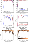 |
Fig. B.21 Observed and calculated line profiles around two preselected Pr II lines for the Sun (top row) and Arcturus (middle row). Black lines: observations, red lines: calculations including preselected spectral lines only, blue lines: calculations including blends from background line list. Bottom row: line profiles generated from observed spectra of selected Gaia FGK benchmark stars. See Sect. 2.3. |
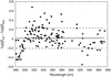 |
Fig. B.22 Comparison between calibrated (cal) and experimental (exp) transition probabilities for Nd II lines in the UVES-580 wavelength range. The data are from Kurucz & Bell (1995) based on Meggers et al. (1975) and from Den Hartog et al. (2003), respectively. The solid black line indicates the mean difference in loggf, and the dashed lines indicate the standard deviation. |
For the two Sm isotopes with non-zero spin HFS A and B constants are available from the experimental work by Masterman et al. (2003) based on collinear fast-ion-beam laser spectroscopy. Their data cover all of the ten levels involved in the preselected Sm II transitions except one (the upper level of the line at 483.7 nm) and are summarised in Table C.11. We note that Masterman et al. (2003) write that they fixed the ratios of A147∕A149 and B147∕B149 for each level tothe values corresponding to the ratios of the nuclear magnetic and electric quadrupole moments (1.213 and − 3.5), respectively. This does not appear to be the case for the B constants, however, for which the ratios for the levels of interest vary between − 3.4 and − 3.7.
B.33 Europium (Z = 63)
For the preselected Eu II lines we rely on the gf-values measured by Lawler et al. (2001c) based on experimental life-times and BFs. In addition, the background line list contains data by Den Hartog et al. (2002) for Eu I, by Zhiguo et al. (2000) for Eu II, and by Meggers et al. (1975) for both ions.
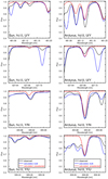 |
Fig. B.23 Comparison of observed and calculated line profiles around four of the preselected Nd II lines for the Sun (left) and Arcturus (right). Black lines: observations, red lines: calculations including preselected spectral lines only, blue lines: calculations including blends from background line list. |
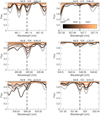 |
Fig. B.24 Line profiles for preselected Nd II lines generated from observed spectra of selected Gaia FGK benchmark stars. See Sect. 2.3. |
The five preselected Eu II lines are rather weak and partly blended in the spectra of the Sun, Arcturus, and other benchmark stars. Figure B.26 shows the line profiles of the two strongest lines, of which the one at 643.8 nm is clearly blended (synflag = N). The line at 664.5 nm might be useful for giant stars at high signal-to-noise ratios (to be decided on a case-by-case basis, synflag = U).
HFS and IS data
Europium occurs in the form of two isotopes (151Eu and 153Eu, with non-zero nuclear spin), each contributing about equally to the Solar System Eu abundance (Table 3). Isotopicshifts for 24 optical Eu II transitions were compiled by Lawler et al. (2001c, their Table 5). These are in general smaller than for Sm II lines and particularly small for the preselected Eu II lines (≲0.02 Å, not resolvedin FTS spectra). Therefore, IS data were not included for Eu II lines in the Gaia-ESO line list.
For four energy levels involved in the preselected Eu II transitions we used the experimental HFS A and B constants by Hühnermann et al. (1992) and Möller et al. (1993), respectively. These are based on the LIF method and are in excellent agreement with the measurements by Sen & Childs (1987) obtained from laser radio frequency double resonance spectroscopy (see compilation by Lawler et al. 2001c, their Table 4). For the remaining three levels we used the LIF data from Villemoes et al. (1992), who give essentially the same values as Hühnermann et al. (1992) and Möller et al. (1993) for these levels. The complete set of HFS data is given in Table C.12.
B.34 Gadolinium (Z = 64) and Dysprosium (Z = 66)
Gd II and Dy II are the heaviest species included in the preselected line list, with one line each (at 486.504 and 516.969 nm, respectively). Laboratory transition probabilities based on the TRLIF-FTS technique have been published for the two lines by Den Hartog et al. (2006) and Wickliffe et al. (2000), respectively, where the latter provide data for Dy I lines as well. In addition to these sources, the background line list contains data for Gd I, Gd II, Dy I, and Dy II from Meggers et al. (1975).
Both of the preselected lines are very weak and blended in the spectra of the Sun, Arcturus, and other benchmark stars and thus are of questionable use for a meaningful abundance analysis (synflag = U). In dwarf stars the Gd II line is located in the red wing of the Hβ line. The line profiles for both transitions are illustrated in Fig. B.27. However, Den Hartog et al. (2006) and Wickliffe et al. (2000) list about 150 and 30 Gd II and Dy II lines, respectively, in the UVES-580 wavelength range (and about ten lines each in the GIRAFFE HR21 range), for which a blending analysis could be done. This analysis should include the parameters of an r-process-rich, metal-poor star.
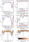 |
Fig. B.25 Observed and calculated line profiles around two preselected Sm II lines for the Sun (top row) and Arcturus (middle row). Black lines: observations, red lines: calculations including preselected spectral lines only, blue lines: calculations including blends from background line list. Bottom row: line profiles generated from observed spectra of selected Gaia FGK benchmark stars. See Sect. 2.3. |
Gadolinium and Dysprosium have several stable isotopes, of which five and four contribute rather evenly to the Solar System Gd and Dy abundances, respectively (Table 3). Both elements have two isotopes with non-zero nuclear spin, giving rise to HFS. Den Hartog et al. (2006) observed partially resolved isotopic andhyperfine structure in the profiles for a few of the Gd II lines in their highest resolution FTS data, and Wickliffe et al. (2000) noticed partially resolved structure for many of the Dy II lines in their FTS spectra. However, most of the lines of both specieswere considered sufficiently narrow to be treated as single component lines in stellar abundance work (Lawler et al. 2009).
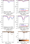 |
Fig. B.26 Observed and calculated line profiles around two preselected Eu II lines for the Sun (top row) and Arcturus (middle row). Black lines: observations, red lines: calculations including preselected spectral lines only, blue lines: calculations including blends from background line list. Bottom row: line profiles generated from observed spectra of selected Gaia FGK benchmark stars. See Sect. 2.3. |
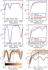 |
Fig. B.27 Observed and calculated line profiles around the preselected Gd II and Dy II lines for the Sun (top row) and Arcturus (middle row). Black lines: observations, red lines: calculations including preselected spectral lines only, blue lines: calculations including blends from background line list. Bottom row: line profiles generated from observed spectra of selected Gaia FGK benchmark stars. See Sect. 2.3. |
Appendix C Hyperfine structure and isotopic splitting data
This appendix provides the HFS and IS data presented in Appendix B for several elements in the form of tables. If not stated otherwise, each table lists level energies E in eV, HFS constantsA and B in units of cm−1, representingmagnetic dipole and electric quadrupole interactions for each level, as well as level designations and references. If applicable, isotopic wavelength shifts are given, in units of cm−1. Subscripts indicate baryon numbers for different isotopes.
HFS constants for 12 Sc I levels.
HFS constants for 53 V I levels.
HFS constants for 35 Mn I levels.
HFS constants for 47 Co I levels measured by Pickering (1996).
HFS constants and isotopic shifts relative to the ground state (4s 2S) for five Cu I levels.
HFS constants for five Ba II levels, for isotopes with non-zero nuclear spin.
HFS constants for nine La II levels.
HFS constant A for 12 Pr II levels.
Wavelength shifts for isotopes with baryon numbers 150 and 142 relative to isotope 144 for the 53 preselected Nd II lines.
HFS constants for 34 out of the 69 Nd II levels involved in the preselected transitions.
HFS constants for nine out of the ten Sm II levels involved in the preselected transitions, for isotopes with non-zero nuclear spin.
HFS constants for seven Eu II levels.
Appendix D Species occurring in the background line list only
The background line list includes a number of lines for species which do not occur in the preselected line list. The references for the gf-values of those lines in the UVES-580 and GIRAFFE HR21 wavelength ranges with an estimated line depth in Arcturus greater than 1% are given in Table D.1 (omitting species with less than five lines).
References for gf-values for species which occur only in the background line list.
Appendix E Theoretical background for collisional broadening data
We discuss three commonly used and presently available options for the calculation of spectral line broadening by collisions with ground state neutral hydrogen atoms. These are:
- 1.
The Unsöld recipe. Lindholm-Foley theory employing the van der Waals long-range interaction potential C6∕R6 as a function of internuclear distance R, where C6 is calculated approximately as formulated by Unsöld (1955).
- 2.
Kurucz calculations. Lindholm-Foley theory as in 1, where C6 is calculated in more detail, as described by Kurucz (1981, p. 76).
- 3.
The ABO theory. Detailed scattering calculations based on potentials from perturbation theory as described by Anstee & O’Mara (1991), and successive expansions by P.S. Barklem and collaborators.
All three methods employ the impact theory (see for example Sect. 4.1 of Barklem 2016, and references therein), and thus the collisionally broadened line profile is described by a Lorentz profile. The long-range dispersion interaction between atoms is given by the van der Waals potential, which may be written in terms of the frequency shift Δν = C6∕R6. In Lindholm-Foley theory (Lindholm 1946; Foley 1946), assuming such a form for the state-dependent dispersive part of the interaction that leads to line broadening, the line width (full width at half-maximum) is given in angular frequency units by
 (E.1)
(E.1)
where  is the mean relative speed, NH the number density of hydrogen atom perturbers, and C6,low and C6,upp are the relevant constants for the interactions between the ground state hydrogen atoms and the atom of interest in the lower and upper states of the transition, respectively. The dispersion coefficient C6 for the interaction between atoms A and B is given by (e.g. Margenau 1939, Sect. C.I.a)
 (E.2)
(E.2)
where  is the energy of level i in atom X, and
  is the oscillator strength for the transition between levels i and j, and the remaining symbols have their usual meaning.
If one of the atoms is a ground-state hydrogen atom, then the energy level separations are at least 10.2 eV, typically much larger than those in the other atom (especially for neutrals). Thus, the sums can be separated and the hydrogen atom part written in terms of the static dipole polarisability of hydrogen in its ground state αH (see Kurucz 1981, p. 76):
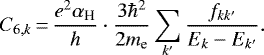 (E.3)
(E.3)
This is the expression used by Kurucz, and the sums are computed over all possible transitions (of the electrons in outer shells), using calculated gf-values calibrated by fits to observed energy levels. These sums are in general not complete, but they “should be complete or nearly so for most strong lines”28. Furthermore, for the calculation of the line width Eq. (E.1) is slightly modified – the maximum value of C6,upp and C6,low is used instead of the difference.
The Unsöld recipe further approximates the summation over all states of the atom of interest by use of the completeness relation (noting that the oscillator strength is related by definition to the dipole operator), and the equation reduces to (Unsöld 1955)
 (E.4)
(E.4)
where ⟨p2⟩ is the mean square radial coordinate of the optical electron on the atom of interest. The value of ⟨p2 ⟩ can be estimated from the result in a hydrogenic atom, which gives ⟨p2⟩ as a simple analytic expression as a function of the effective principle quantum number n* and the orbital angular momentum quantum number l (see Bates & Damgaard 1949, p. 111). Adopting this expression and neglecting the dependence on l for simplicity, one obtains
 (E.5)
(E.5)
where a0 is the Bohr radius, Z is the atomic number, and Ne is the total number of electrons for a given species (i.e. Z − Ne + 1 = 1, 2, … for neutral, singly ionised, … species, respectively).
The effective principal quantum number is defined by the hydrogenic formula for the binding energy of the electron nl,  Rydbergs. For a series of (core)-nl levels, the binding energy of the electron is given by Enl = Elimit − Ei, where Elimit is the series limit energy for the appropriate core. For the case of a single excited electron outside a core in the ground state of the next higher ionisation stage, Elimit is equal to the ionisation potential Eion of the absorbing species. However, the parent configuration of the state of interest may correspond to an excited state of the core. In that case, the energy of the excited core state EP (relative to the core ground state) must be added to the ionisation potential when calculating n*, that is, Elimit = Eion + EP, in order to obtain the correct binding energy for the optical electron. Thus, for level i with energy Ei, the effective principal quantum number should be calculated according to
  , where EH is the ionisation potential of hydrogen. Correct calculation of the binding energy can be very important in complex atoms such as Ca and Fe (see, e.g. Barklem et al. 2000a), but requires detailed information about the electron configurations. As far as we know, this has never been taken into account in the context of the Unsöld recipe, probably in part due to the fact that then the simplicity of the calculation is largely lost, as one needs electron configuration information. In this work we adopt the same principle, and always adopt Elimit = Eion for the Unsöld recipe calculations; however, the correct values are adopted when employing the ABO theory, which is now described.
The ABO theory is a modification of the line-broadening theory by Brueckner (1971), and is described in Anstee & O’Mara (1991). The main improvement with respect to theories based on the van der Waals potential is that interactions at intermediate internuclear distances are more accurately described. The calculation of the interaction energy does not employ the multipole expansion and thus is more appropriate for distances where the electronic wavefunctions overlap moderately. Intermediate-range interactions make an important contribution to the line-broadening cross sections. The second-most important improvement is that each m state (|m| = 0, 1, …l) is treated, thus removing the averaging over phases found in the Lindholm-Foley theory. ABO theory applies a model of the collision dynamics that includes the m-substates explicitly, and also includes the relative rotation of the atoms during the collision. Anstee & O’Mara (1991) showed that neglect of these effects leads to an overestimate of the broadening by about 30%. See Anstee & O’Mara (1991) for more details, and Barklem (2016) for more references and a more detailed review of the differences between Lindholm-Foley and ABO theory.
Publications of line-broadening data from ABO theory and applicable ranges of effective principal quantum numbers for neutral species.
For neutral species ABO theory can be applied to calculate cross-sections in general for transitions between different l states. Cross-sections for transitions between l = 0, 1, 2, 3 (s, p, d, f, respectively) states are presented in the publications listed in Table E.1. These tabulate the line-broadening cross sections σ for a specific value of the relative speed, v0 = 104 m s−1, as a function of the effective principal quantum numbers n* of the relevant levels. The dependence of σ on the collision speed v is parametrised by a power-law exponent α, which is also tabulated for the different n* combinations. We note that the ABO theory only applies to transitions that obey the one-electron selection rule Δl = ± 1. However, in complex atoms one often finds situations where the optical electron (the outermost electron that determines the interaction potential) in the lower and upper states does not obey this rule, and one has transitions where the optical electron is in the same l state throughout the transition, such as p–p. In these cases, since the upper state dominates the broadening, data can be estimated by taking a corresponding transition with the same upper state, for example s–p instead of p–p.
Barklem et al. (2000b) determined effective principal quantum numbers, accounting correctly for core excitations, for 4872 lines of 23 neutral species from Li to Ni and obtained a list of broadening data by interpolation in the tables published earlier (see Table E.1). The list was constructed for all neutral species in the wavelength region between 230 and 1300 nm, for which all of the required information was available in the NIST Atomic Spectra Database at that time, and for which the transition type and the n* values were within the table limits. An additional line selection criterion was loggf ≥−5, as lines with lower gf-values were assumed to be unaffected by this type of broadening.
For ionised species it is not possible to tabulate the broadening data in a general way, while retaining the same accuracy as for neutrals. Broadening data were calculated for a few strong lines of Mg II and Ca II by Barklem & O’Mara (1998) and of Be II, Sr II, and BaII by Barklem & O’Mara (2000), and these data were included in Barklem et al. (2000b). Since then, over 24 000 Fe II lines were calculated by Barklem & Aspelund-Johansson (2005), and over 13 000 Cr II lines by P.S. Barklem29. All of the published broadening data (cross sections σ and velocity parameters α) for specific lines of neutral and ionised species from the ABO data are made available through the VALD database. Using the speed dependence of σ parametrised by α together with a Maxwell distribution, the integration over velocity leads to the following expression for line width:
 (E.6)
(E.6)
where Γ(x) is the Gamma function and v0 = 104 ms−1.
Finally, we note that in all cases, collisions with ground state neutral helium can additionally be taken into account in an approximate way by replacing NH with NH+cNHe, where NHe is the number density of helium atoms. The coefficient c ≈ 0.41 accounts for differences in the polarisability and for the mass (and thus mean velocity) of He.
Appendix F Broadening data comparisons
The ABO theory has been extensively tested through comparisons with the solar spectrum (e.g. all papers in Table E.1, as well as Barklem & O’Mara 2001) and with more detailed calculations where available (e.g. Kerkeni et al. 2004). Based on these comparisons the ABO theory is estimated to be accurate to better than 20 to 30%, though in some cases it may be significantly better (see Anstee & O’Mara 1995). On the other hand, the Unsöld recipe, based on the Lindholm-Foley theory and the van der Waals interaction, is well-known to be typically only reliable to about a factor of 2. See Barklem (2016) for a more detailed discussion and comparison of the various theories and the evidence for their accuracies. However, the conclusion is that the evidence indicates that the ABO theory is the most reliable of the three methods considered here.
In Fig. F.1 we compare line widths computed with the three different options described in Appendix E for lines of a representative neutral species–Fe I–at a representative temperature of 6000 K. Lines for which both Kurucz calculations and ABO data are available were extracted from the VALD database in the wavelength range 480 to 680 nm (on 2 Jul 2012). The figure shows the ratio of the ABO width to the width from the Kurucz line list and to the Unsöld width (the latter calculated from Eqs. (E.5) and (E.1)). On the basis that the ABO value represents the most realistic line width, the ratio can be seen as an ‘enhancement factor’ to be applied to the Kurucz or Unsöld γ-values. The ratio is shown as a function of lower level energy, and different symbols represent different transition types (combinations of l quantum numbers).
 |
Fig. F.1 Ratio of collisional line width γ calculated from ABO theory to line width from van der Waals theory using Kurucz or Unsöld C6 values, for Fe I lines of transition types s–p, p–s, and p–d, at a temperature of 6000 K, as a function of lower level energy Elow. |
 |
Fig. F.2 Ratio of collisional line width γ calculated from ABO theory to line width from van der Waals theory using Kurucz or Unsöld C6 values, for Fe II lines of transition types s–p, p–s, p–d (upper panel), d–p and p–p (lower panel), at a temperature of 6000 K, as a function of lower level energy Elow. |
A large spread in the ratios is evident for high values of the excitation energy (Elow ≳ 2.8 eV), for both Kurucz and Unsöld values. For p–s and p–d transitions the Kurucz ratios cluster around 2, while the Unsöld ratios cluster at two different values (close to 2.5 for p–s and 1.5 for p–d), and a few p–s and p–d lines are seen at 1.5 and 0.5, respectively. For the s–p transitions with Elow ≳ 2.8 eV all Unsöld ratios are less than 1, implying that a ‘reduction factor’ would be required for Unsöld values with respect to ABO theory. Low ABO values are obtained when the transition takes place involving one or two levels with excited cores. In such a case, the value of Elimit in the calculation of the effective principal quantum number n* is increased with respect to if Eion is used (as typically done in the Unsöld recipe), which implies a smaller n* value and hence a decreased σ. On the other hand, the Kurucz ratios cluster around 1 and 1.5. Finally, for lines with Elow < 2.8 eV (s–p transitions) the Kurucz ratios gradually increase from 1 to 1.5, while the Unsöld ratios are constant at around 1.5.
Figure F.2 shows a similar comparison for lines of a representative ionised species–Fe II. We see an equally complex pattern of enhancements of line widths, in particular for Unsöld values at high excitation energies (Elow ≳ 7.3 eV). Kurucz ratios are close to 1 for Elow < 7.3 eV (all of these are s–p, p–s, or d–p transitions).
Appendix G Broadening data for preselected lines
G.1 Neutral species
In view of the comparisons presented in Appendix F it seems impossible to define a universal enhancement factor for broadening data calculated with the Unsöld recipe. Thus, it is desirable to use ABO theory data whenever possible. ABO data were available from Barklem et al. (2000b) for about 70% of the preselected lines in the Gaia-ESO line list (see Sect. 2.1 and Appendix B for a description of the preselected line list). We aimed at increasing the percentage at least for the lines with otherwise high-quality data. New ABO data were determined for most of the Y/Y lines and a few Y/U, U/Y, and U/U lines lacking such data. These were mostly lines of Fe I, and a few lines of C I, Si I, Ca I, Sc I, Cr I, Zn I, Zr I, and Mo I.
For these lines we extracted the atomic data from the NIST Atomic Spectra Database required to calculate the effective principal quantum number n*. In particular, term designations and electron configurations of the levels involved in the transitions were obtained. We also determined the electron configuration of the parent terms and checked whether they deviated from the ground states of the corresponding singly ionised species listed in Table G.1. In that case the excitation energy of the parent term was determined and added to the ionisation energy in the calculation of the effective principal quantum number. All of these input data are given in Table G.2.
We then interpolated in the cross-section tables of the ABO publications listed in Table E.1, where possible. The interpolation was done using the code widthcomp (version 2.0) from the abo-cross package (Barklem et al. 2015). For a few lines, the n* values (given in Table G.3) fall outside the range of the relevant cross-section interpolation table. In these cases the cross sections were calculated individually for each line. For example, this occurs for eight of the Fe I lines which are d–p transitions. In all cases both states have a parent configuration corresponding to an excited state of Fe II (see Table G.2), resulting in  , and
, and  (see Table G.3). The cross sections calculated directly for these lines are about 300–400 atomic units. The results for all lines are given in Table G.3. In total, we determined new ABO values for 41 lines: 28 Fe lines (s–p, p–s, p–d, d–p), two C lines (p–p, p–d), three, two, and one s–p lines of Si, Sc, and Cr, respectively, and five lines for elements with Z > 28 (s–p and p–s lines of Zn, Zr, and Mo). For the two Ca lines it was not possible to determine reliable ABO values.
Ionisation energies Eion of neutral species listed in Tables G.2 and G.3 and ground states of corresponding singly ionised species (Martin et al. 2011; Ralchenko et al. 2011).
G.2 Ionised species
All lines of Cr II and Fe II in the preselected line list have ABO data (Barklem & Aspelund-Johansson 2005). All four Ba II lines (Appendix B.27) have ABO data (Barklem & O’Mara 1998, 2000) as well. For Ca II (Appendix sectionlinking B.10) only the three NIR triplet lines have ABO data (Barklem & O’Mara 1998). For the other preselected Ca II lines calculations by Kurucz (2010b) are available. These are p–d, d–f, and f–g transitions with rather high excitation potentials (Elow > 7 eV).
No ABO theory calculations are available for the remaining ionised species. For the two preselected Si II lines (s–p transitions with Elow = 8.1 eV), calculations by Kurucz (2012) are available. For the lines of Sc II (s–p, d–s), Ti II (s–p, d–p), and Y II (d–p), calculations by Kurucz (2009, 2010b, 2011) are available, respectively. The remaining species and transitions have no data. These are Zr II (s–p, d–p) and the rare-earth elements La II (s–d, d–d), Ce II (s–p, d–p, d–d), Pr II (d–p, d–d), Nd II (s–s, s–d, s–?, d–p, d–d, d–?), Sm II (s–s, s–p), Eu II (d–p), Gd II (s–s), and Dy II (s–p). Here “?” means that there are some transitions for which the upper level l state is unknown. All lines of the ionised species without ABO data (except for Si II and Ca II) have low excitation potentials (Elow ≲ 3 eV).
Atomic data for high-quality lines of neutral species in the preselected Gaia-ESO line list which are not included in Barklem et al. (2000b).
Effective principal quantum numbers n*, and ABO theory broadening data, for high-quality lines of neutral species, which are not included in Barklem et al. (2000b).
Appendix H Recommendations and conclusions for collisional broadening data
For neutral species in the preselected line list, we recommend to use the ABO theory cross-sections provided with the Gaia-ESO line list. These include the newly derived values given in Table G.3 and should be used with Eq. (E.6) to compute line widths. The number of lines with ABO data per species and for various quality classifications is given in Table 1. For future applications of the line list, the ABO theory interpolation work should be extended to the remaining preselected neutral lines. These are 103 Fe I lines and about 200 lines of other species (e.g. 42 Si I and 21 Ti I lines, and about ten lines each of neutral Na, Mg, S, Cr, Mn, Co, Ni, Sr, Zr, Nb). For ionised species Fig. F.2 indicates that broadening calculations by Kurucz are close to the ABO theory data for low excitation energies. Although we do not know the limit for Elow for species other than Fe II, we recommend to use Kurucz data for the preselected Sc II, Ti II, and Y II lines, based on their rather low Elow values30. For the rare-earth species we recommend to use the Unsöld recipe (Eqs. (E.5) and (E.1)) with an enhancement factor for the line width of 1.5, again based on Fig. F.2.
For all lines without broadening data the parameter value was set to zero in the line list. Finally, we note that collisional broadening does not significantly affect the equivalent widths W of spectral lines with low ratios of logW∕λ. As a rough guideline, we can derive a limit of logW∕λ ≲−4.8 from Fig. 2 in Warner (1967), which corresponds to W ≲75–110 mÅ for the UVES-580 wavelength range and W ≲130–145 mÅ for the wavelength range of the GIRAFFE HR21 setting. For such lines the value of the line broadening constant or the theory used should be less relevant.
References
- Ahmad, S. A., & Saksena, G. D. 1981, Spectrochim. Acta, 36, 943 [NASA ADS] [CrossRef] [Google Scholar]
- Aldenius, M., Tanner, J. D., Johansson, S., Lundberg, H., & Ryan, S. G. 2007, A&A, 461, 767 [NASA ADS] [CrossRef] [EDP Sciences] [Google Scholar]
- Aldenius, M., Lundberg, H., & Blackwell-Whitehead, R. 2009, A&A, 502, 989 [NASA ADS] [CrossRef] [EDP Sciences] [Google Scholar]
- Allard, N. F., Kielkopf, J. F., Cayrel, R., & van’t Veer-Menneret C. 2008, A&A, 480, 581 [NASA ADS] [CrossRef] [EDP Sciences] [Google Scholar]
- Anstee, S. D., & O’Mara, B. J. 1991, MNRAS, 253, 549 [Google Scholar]
- Anstee, S. D., & O’Mara, B. J. 1995, MNRAS, 276, 859 [NASA ADS] [CrossRef] [Google Scholar]
- Arnesen, A., Bengtsson, A., Hallin, R., et al. 1977, Phys. Scr., 16, 31, aBH [CrossRef] [Google Scholar]
- Asplund, M., Grevesse, N., Sauval, A. J., & Scott, P. 2009, ARA&A, 47, 481 [NASA ADS] [CrossRef] [Google Scholar]
- Baertschi, P. 1976, Earth Planet. Sci. Lett., 31, 341 [NASA ADS] [CrossRef] [Google Scholar]
- Baluja, K. L., & Zeippen, C. J. 1988, J. Phys. B At. Mol. Phys., 21, 1455 [NASA ADS] [CrossRef] [Google Scholar]
- Bard, A., & Kock, M. 1994, A&A, 282, 1014 [NASA ADS] [Google Scholar]
- Bard, A., Kock, A., & Kock, M. 1991, A&A, 248, 315 [NASA ADS] [Google Scholar]
- Barklem, P. S. 2016, A&ARv, 24, 9 [NASA ADS] [CrossRef] [Google Scholar]
- Barklem, P. S., & Aspelund-Johansson, J. 2005, A&A, 435, 373, (BA-J) [NASA ADS] [CrossRef] [EDP Sciences] [Google Scholar]
- Barklem, P. S., & Collet, R. 2016, A&A, 588, A96 [NASA ADS] [CrossRef] [EDP Sciences] [Google Scholar]
- Barklem, P. S., & O’Mara, B. J. 1997, MNRAS, 290, 102 [Google Scholar]
- Barklem, P. S., & O’Mara, B. J. 1998, MNRAS, 300, 863 [NASA ADS] [CrossRef] [Google Scholar]
- Barklem, P. S., & O’Mara, B. J. 2000, MNRAS, 311, 535 [NASA ADS] [CrossRef] [Google Scholar]
- Barklem, P. S., & O’Mara, B. J. 2001, J. Phys. B At. Mol. Opt. Phys., 34, 4785 [NASA ADS] [CrossRef] [Google Scholar]
- Barklem, P. S., O’Mara, B. J., & Ross, J. E. 1998, MNRAS, 296, 1057 [Google Scholar]
- Barklem, P. S., Piskunov, N., & O’Mara, B. J. 2000a, A&A, 363, 1091 [NASA ADS] [Google Scholar]
- Barklem, P. S., Piskunov, N., & O’Mara, B. J. 2000b, A&AS, 142, 467 [NASA ADS] [CrossRef] [EDP Sciences] [MathSciNet] [PubMed] [Google Scholar]
- Barklem, P. S., Anstee, S. D., & O’Mara, B. J. 2015, Astrophysics Source Code Library [record ascl:1507.007] [Google Scholar]
- Başar, G., Başar, G., Acar, G., Öztürk, I. K., & Kröger, S. 2003, Phys. Scr., 67, 476 [NASA ADS] [CrossRef] [Google Scholar]
- Başar, G., Başar, F. G., Öztürk, İ. K., & Kröger, S. 2004, Phys. Scr., 69, 189 [NASA ADS] [CrossRef] [Google Scholar]
- Bates, D. R., & Damgaard, A. 1949, Phil. Trans. R. Soc. A Math., Phys. Eng. Sci., 242, 101 [Google Scholar]
- Becker, W., Blatt, R., & Werth, G. 1981, in Precision Measurement and Fundamental Constants, eds. B. N. Taylor & W. D. Phillips, 99 [Google Scholar]
- Bergemann, M., Ruchti, G. R., Serenelli, A., et al. 2014, A&A, 565, A89 [NASA ADS] [CrossRef] [EDP Sciences] [Google Scholar]
- Bergeson, S. D., & Lawler, J. E. 1993, J. Opt. Soc. Am. B Opt. Phys., 10, 794 [NASA ADS] [CrossRef] [Google Scholar]
- Bergström, H., Peng, W. X., & Persson, A. 1989, Z. Phys. D At. Mol. Clusters, 13, 203 [CrossRef] [Google Scholar]
- Biémont, E. 1973, Bull. Soc. R. Sci. Liege, 42, 206 [Google Scholar]
- Biemont, E., & Godefroid, M. 1980, A&A, 84, 361 [NASA ADS] [Google Scholar]
- Biemont, E., Grevesse, N., Hannaford, P., & Lowe, R. M. 1981, ApJ, 248, 867 [NASA ADS] [CrossRef] [Google Scholar]
- Biemont, E., Grevesse, N., Kwiatkovski, M., & Zimmermann, P. 1984, A&A, 131, 364 [NASA ADS] [Google Scholar]
- Biemont, E., Quinet, P., & Zeippen, C. J. 1993, A&AS, 102, 435 [NASA ADS] [Google Scholar]
- Biémont, E., Dutrieux, J., Martin, I., & Quinet, P. 1998, J. Phys. B At. Mol. Phys., 31, 3321 [NASA ADS] [CrossRef] [Google Scholar]
- Biémont, E., Lefèbvre, P., Quinet, P., Svanberg, S., & Xu, H. L. 2003, Eur. Phys. J. D, 27, 33 [NASA ADS] [CrossRef] [EDP Sciences] [Google Scholar]
- Biémont, É., Blagoev, K., Engström, L., et al. 2011, MNRAS, 414, 3350 [NASA ADS] [CrossRef] [Google Scholar]
- Bizzarri, A., Huber, M. C. E., Noels, A., et al. 1993, A&A, 273, 707 [NASA ADS] [Google Scholar]
- Bizzarro, M., Paton, C., Larsen, K., et al. 2011, J. Anal. At. Spectrom., 26, 565 [CrossRef] [Google Scholar]
- Blackwell, D. E., Ibbetson, P. A., Petford, A. D., & Shallis, M. J. 1979a, MNRAS, 186, 633 [NASA ADS] [CrossRef] [Google Scholar]
- Blackwell, D. E., Petford, A. D., & Shallis, M. J. 1979b, MNRAS, 186, 657 [NASA ADS] [CrossRef] [Google Scholar]
- Blackwell, D. E., Petford, A. D., Shallis, M. J., & Leggett, S. 1982a, MNRAS, 199, 21 [CrossRef] [Google Scholar]
- Blackwell, D. E., Petford, A. D., Shallis, M. J., & Simmons, G. J. 1982b, MNRAS, 199, 43 [NASA ADS] [CrossRef] [Google Scholar]
- Blackwell, D. E., Petford, A. D., & Simmons, G. J. 1982c, MNRAS, 201, 595 [NASA ADS] [CrossRef] [Google Scholar]
- Blackwell, D. E., Menon, S. L. R., & Petford, A. D. 1983, MNRAS, 204, 883 [NASA ADS] [CrossRef] [Google Scholar]
- Blackwell, D. E., Menon, S. L. R., & Petford, A. D. 1984, MNRAS, 207, 533 [NASA ADS] [CrossRef] [Google Scholar]
- Blackwell, D. E., Booth, A. J., Haddock, D. J., Petford, A. D., & Leggett, S. K. 1986, MNRAS, 220, 549 [NASA ADS] [CrossRef] [Google Scholar]
- Blackwell-Whitehead, R. J., Xu, H. L., Pickering, J. C., Nave, G., & Lundberg, H. 2005a, MNRAS, 361, 1281 [NASA ADS] [CrossRef] [Google Scholar]
- Blackwell-Whitehead, R. J., Pickering, J. C., Pearse, O., & Nave, G. 2005b, ApJS, 157, 402 [NASA ADS] [CrossRef] [Google Scholar]
- Blackwell-Whitehead, R., & Bergemann, M. 2007, A&A, 472, L43 [NASA ADS] [CrossRef] [EDP Sciences] [Google Scholar]
- Blaise, J., Wyart, J.-F., Tahar Djerad, M., & Ben Ahmed Z. 1984, Phys. Scr., 29, 119 [CrossRef] [Google Scholar]
- Blanco, F., Botho, B., & Campos, J. 1995, Phys. Scr., 52, 628 [NASA ADS] [CrossRef] [Google Scholar]
- Blanco-Cuaresma, S., Soubiran, C., Jofré, P., & Heiter, U. 2014, A&A, 566, A98 [NASA ADS] [CrossRef] [EDP Sciences] [Google Scholar]
- Booth, A. J., Blackwell, D. E., Petford, A. D., & Shallis, M. J. 1984, MNRAS, 208, 147 [NASA ADS] [CrossRef] [Google Scholar]
- Bord, D. J., Barisciano, Jr. L. P., & Cowley, C. R. 1996, MNRAS, 278, 997 [NASA ADS] [CrossRef] [Google Scholar]
- Bourauel, C., Rupprecht, W., & Büttgenbach, S. 1987, Z. Phys. D At. Mol. Clusters, 7, 129 [CrossRef] [Google Scholar]
- Bridges, J. M., & Kornblith, R. L. 1974, ApJ, 192, 793 [NASA ADS] [CrossRef] [Google Scholar]
- Brodzinski, T., Kronfeldt, H.-D., Kropp, J.-R., & Winkler, R. 1987, Z. Phys. D Atoms Mol. Clusters, 7, 161 [CrossRef] [Google Scholar]
- Brooke, J. S. A., Bernath, P. F., Schmidt, T. W., & Bacskay, G. B. 2013, J. Quant. Spectr. Rad. Transf., 124, 11 [NASA ADS] [CrossRef] [Google Scholar]
- Brooke, J. S. A., Ram, R. S., Western, C. M., et al. 2014, ApJS, 210, 23 [NASA ADS] [CrossRef] [Google Scholar]
- Brown, J. A., Sneden, C., Lambert, D. L., & Dutchover, Jr. E. 1989, ApJS, 71, 293 [CrossRef] [Google Scholar]
- Brueckner, K. A. 1971, ApJ, 169, 621 [NASA ADS] [CrossRef] [Google Scholar]
- Butler, K., & Zeippen, C. J. 1991, J. Phys. IV France, 01, C1 [CrossRef] [EDP Sciences] [Google Scholar]
- Butler, K., Mendoza, C., & Zeippen, C. J. 1993, J. Phys. B At. Mol. Phys., 26, 4409 [NASA ADS] [CrossRef] [Google Scholar]
- Cardon, B. L., Smith, P. L., Scalo, J. M., Testerman, L., & Whaling, W. 1982, ApJ, 260, 395 [NASA ADS] [CrossRef] [Google Scholar]
- Carlsson, J., Sturesson, L., & Svanberg, S. 1989, Z. Phys. D Atoms Mol. Clusters, 11, 287 [NASA ADS] [CrossRef] [Google Scholar]
- Casamiquela, L., Carrera, R., Jordi, C., et al. 2016, MNRAS, 458, 3150 [NASA ADS] [CrossRef] [Google Scholar]
- Casimir, H. 1936, On the Interaction Between Atomic Nuclei and Electrons, Archives du musée Teyler (Dordrecht: Springer Netherlands) [Google Scholar]
- Chang, T.-L., & Li, W.-J. 1990, Chin. Sci. Bull., 35, 290 [Google Scholar]
- Chang, T. N.,& Tang, X. 1990, J. Quant. Spectr. Rad. Transf., 43, 207 [NASA ADS] [CrossRef] [Google Scholar]
- Chang, T. L., Qian, Q.-Y., Zhao, M.-T., & Wang, J. 1994, Int. J. Mass Spectrom. Ion Process., 139, 95 [NASA ADS] [CrossRef] [Google Scholar]
- Chang, T.-L., Qian, Q.-Y., Zhao, M.-T., Wang, J., & Lang, Q.-Y. 1995, Int. J. Mass Spectrom. Ion Process., 142, 125 [NASA ADS] [CrossRef] [Google Scholar]
- Chang, T.-L., Li, W.-J., Zhao, M.-T., Wang, J., & Qian, Q.-Y. 2001, Int. J. Mass Spectrom., 207, 13 [NASA ADS] [CrossRef] [Google Scholar]
- Chang, T.-L., Zhao, M.-T., Li, W.-J., Wang, J., & Qian, Q.-Y. 2002, Int. J. Mass Spectrom., 218, 167 [NASA ADS] [CrossRef] [Google Scholar]
- Childs, W. J. 1971, Phys. Rev. A, 4, 1767 [NASA ADS] [CrossRef] [Google Scholar]
- Childs, W. J., Poulsen, O., Goodman, L. S., & Crosswhite, H. 1979, Phys. Rev. A, 19, 168 [NASA ADS] [CrossRef] [Google Scholar]
- Cochrane, E. C. A., Benton, D. M., Forest, D. H., & Griffith, J. A. R. 1998, J. Phys. B At. Mol. Phys., 31, 2203 [NASA ADS] [CrossRef] [Google Scholar]
- Cocke, C. L., Stark, A., & Evans, J. C. 1973, ApJ, 184, 653 [NASA ADS] [CrossRef] [Google Scholar]
- Collins, T. L., Rourke, F. M., & White, F. A. 1957, Phys. Rev., 105, 196 [NASA ADS] [CrossRef] [Google Scholar]
- Condon, E. U., & Shortley, G. H. 1935, The Theory of Atomic Spectra (University Press, the University of Michigan) [Google Scholar]
- Cooper, J. C., Gibson, N. D., & Lawler, J. E. 1997, J. Quant. Spectr. Rad. Transf., 58, 85 [NASA ADS] [CrossRef] [Google Scholar]
- Corliss, C. H., & Bozman, W. R. 1962, NBS Monograph, Experimental transition probabilities for spectral lines of seventy elements; derived from the NBS Tables of spectral-line intensities, eds. C. H. Corliss, & W. R. Bozman (US Government Printing Office), 53 [Google Scholar]
- Corney, A., & Williams, O. M. 1972, J. Phys. B At. Mol. Phys., 5, 686 [NASA ADS] [CrossRef] [Google Scholar]
- Cowley, C. R. 1973, J. Res. NBS, 77A, 419 [CrossRef] [Google Scholar]
- Cowley, C. R., & Corliss, C. H. 1983, MNRAS, 203, 651 [NASA ADS] [CrossRef] [Google Scholar]
- Das, D., & Natarajan, V. 2008, J. Phys. B At. Mol. Phys., 41, 035001 [CrossRef] [Google Scholar]
- Davidson, M. D., Snoek, L. C., Volten, H., & Doenszelmann, A. 1992, A&A, 255, 457 [NASA ADS] [Google Scholar]
- Davis, S. J., Wright, J. J., & Balling, L. C. 1971, Phys. Rev. A, 3, 1220 [NASA ADS] [CrossRef] [Google Scholar]
- de Laeter, J. R., & Bukilic, N. 2005, Int. J. Mass Spectrom., 244, 91 [NASA ADS] [CrossRef] [Google Scholar]
- de Laverny, P., Recio-Blanco, A., Worley, C. C., & Plez, B. 2012, A&A, 544, A126 [NASA ADS] [CrossRef] [EDP Sciences] [Google Scholar]
- Dembczyński, J., Ertmer, W., Johann, U., Penselin, S., & Stinner, P. 1979, Z. Phys. A Hadrons Nuclei, 291, 207 [CrossRef] [Google Scholar]
- den Hartog, E. A., Curry, J. J., Wickliffe, M. E., & Lawler, J. E. 1998, Sol. Phys., 178, 239 [NASA ADS] [CrossRef] [Google Scholar]
- Den Hartog, E. A., Wickliffe, M. E., & Lawler, J. E. 2002, ApJS, 141, 255 [NASA ADS] [CrossRef] [Google Scholar]
- Den Hartog, E. A., Lawler, J. E., Sneden, C., & Cowan, J. J. 2003, ApJS, 148, 543 [Google Scholar]
- Den Hartog, E. A., Herd, M. T., Lawler, J. E., et al. 2005, ApJ, 619, 639, (DHL) [NASA ADS] [CrossRef] [Google Scholar]
- Den Hartog, E. A., Lawler, J. E., Sneden, C., & Cowan, J. J. 2006, ApJS, 167, 292 [NASA ADS] [CrossRef] [Google Scholar]
- Den Hartog, E. A., Lawler, J. E., Sobeck, J. S., Sneden, C., & Cowan, J. J. 2011, ApJS, 194, 35 [NASA ADS] [CrossRef] [Google Scholar]
- Den Hartog, E. A., Ruffoni, M. P., Lawler, J. E., et al. 2014, ApJS, 215, 23 [NASA ADS] [CrossRef] [Google Scholar]
- De Silva, G. M., Freeman, K. C., Bland-Hawthorn, J., et al. 2015, MNRAS, 449, 2604 [NASA ADS] [CrossRef] [MathSciNet] [Google Scholar]
- Ding, T., Valkiers, S., Kipphardt, H., et al. 2001, Geochim. Cosmochim. Acta, 65, 2433 [NASA ADS] [CrossRef] [Google Scholar]
- Doerr, A., & Kock, M. 1985, J. Quant. Spectr. Rad. Transf., 33, 307 [NASA ADS] [CrossRef] [Google Scholar]
- Drozdowski, R., Ignaciuk, M., Kwela, J., & Heldt, J. 1997, Z. Phys. D Atoms Mol. Clusters, 41, 125 [CrossRef] [Google Scholar]
- Dulick, M., Bauschlicher, Jr. C. W., Burrows, A., et al. 2003, ApJ, 594, 651 [NASA ADS] [CrossRef] [Google Scholar]
- Duquette, D. W., & Lawler, J. E. 1982, Phys. Rev. A, 26, 330 [NASA ADS] [CrossRef] [Google Scholar]
- Duquette, D. W., & Lawler, J. E. 1985, J. Opt. Soc. Am. B Opt. Phys., 2, 1948 [NASA ADS] [CrossRef] [Google Scholar]
- Duquette, D. W., Salih, S., & Lawler, J. E. 1982a, Phys. Rev. A, 26, 2623 [NASA ADS] [CrossRef] [Google Scholar]
- Duquette, D. W., Salih, S., & Lawler, J. E. 1982b, J. Phys. B At. Mol. Phys., 15, L897 [NASA ADS] [CrossRef] [Google Scholar]
- Duquette, D. W., den Hartog, E. A., & Lawler, J. E. 1986, J. Quant. Spectr. Rad. Transf., 35, 281 [NASA ADS] [CrossRef] [Google Scholar]
- El-Kashef, H., & Ludwig, N. 1992, Phys. B Condens. Matter, 179, 103 [NASA ADS] [CrossRef] [Google Scholar]
- Ertmer, W., & Hofer, B. 1976, Z. Phys. A Hadrons Nuclei, 276, 9 [CrossRef] [Google Scholar]
- Eugster, O., Tera, F., & Wasserburg, G. J. 1969, J. Geophys. Res., 74, 3897 [NASA ADS] [CrossRef] [Google Scholar]
- Eugster, O., Tera, F., Burnett, D. S., & Wasserburg, G. J. 1970, J. Geophys. Res., 75, 2753 [NASA ADS] [CrossRef] [Google Scholar]
- Fedchak, J. A., Den Hartog, E. A., Lawler, J. E., et al. 2000, ApJ, 542, 1109 [NASA ADS] [CrossRef] [Google Scholar]
- Fischer, W., Hühnermann, H., & Kollath, K.-J. 1967, Z. Phys., 200, 158 [Google Scholar]
- Fivet, V., Quinet, P., Palmeri, P., et al. 2009, MNRAS, 396, 2124 [NASA ADS] [CrossRef] [Google Scholar]
- Flesch, G. D., Capellen, J., & Svec, H. J. 1966, Adv. Mass Spectrom., 3, 571 [Google Scholar]
- Foley, H. M. 1946, Phys. Rev., 69, 616 [NASA ADS] [CrossRef] [Google Scholar]
- Froese Fischer, C., & Tachiev, G. 2012, Multiconfiguration Hartree-Fock and Multiconfiguration Dirac-Hartree-Fock Collection, Version 2, http://physics.nist.gov/mchf/ [Google Scholar]
- Fuhr, J. R., & Wiese, W. L. 2006, J. Phys. Chem. Ref. Data, 35, 1669 [NASA ADS] [CrossRef] [Google Scholar]
- Fuhr, J. R., Martin, G. A., & Wiese, W. L. 1988, J. Phys. Chem. Ref. Data, 17, 4 [Google Scholar]
- Furmann, B., Ruczkowski, J., Stefańska, D., Elantkowska, M., & Dembczyński, J. 2008, J. Phys. B At. Mol. Phys., 41, 215004 [CrossRef] [Google Scholar]
- Galavis, M. E., Mendoza, C., & Zeippen, C. J. 1997, A&AS, 123, 159 [NASA ADS] [CrossRef] [EDP Sciences] [Google Scholar]
- Gallagher, A. 1967, Phys. Rev., 157, 24 [NASA ADS] [CrossRef] [Google Scholar]
- García, G., & Campos, J. 1988, J. Quant. Spectr. Rad. Transf., 39, 477 [Google Scholar]
- Garz, T. 1973, A&A, 26, 471 [NASA ADS] [Google Scholar]
- Garz, T., & Kock, M. 1969, A&A, 2, 274 [NASA ADS] [Google Scholar]
- Gilmore, G., Randich, S., Asplund, M., et al. 2012, The Messenger, 147, 25 [NASA ADS] [Google Scholar]
- Ginibre, A. 1989, Phys. Scr, 39, 694 [NASA ADS] [CrossRef] [Google Scholar]
- Gonfiantini, R., de Bievre, P., Valkiers, S., & Taylor, P. D. P. 1997, IEEE Trans. Instrum. Measur., 46, 566 [CrossRef] [Google Scholar]
- Gough, D. S., Hannaford, P., & Lowe, R. M. 1982, J. Phys. B At. Mol. Phys., 15, L431 [NASA ADS] [CrossRef] [Google Scholar]
- Gough, D. S., Hannaford, P., & Lowe, R. M. 1983, J. Phys. B. At. Mol. Phys., 16, 785 [NASA ADS] [CrossRef] [Google Scholar]
- Gramlich, J. W., Machlan, L. A., Barnes, I. L., & Paulsen, P. J. 1989, J. Res. Natl. Bur. Std., 94, 347 [Google Scholar]
- Gray, D. F. 2005, The Observation and Analysis of Stellar Photospheres (Cambridge, UK: Cambridge University Press) [CrossRef] [Google Scholar]
- Grevesse, N., Blackwell, D. E., & Petford, A. D. 1989, A&A, 208, 157 [NASA ADS] [Google Scholar]
- Grevesse, N., Asplund, M., & Sauval, A. J. 2007, Space Sci. Rev., 130, 105 [Google Scholar]
- Grevesse, N., Scott, P., Asplund, M., & Sauval, A. J. 2015, A&A, 573, A27 [NASA ADS] [CrossRef] [EDP Sciences] [Google Scholar]
- Guiglion, G., de Laverny, P., Recio-Blanco, A., et al. 2016, A&A, 595, A18 [NASA ADS] [CrossRef] [EDP Sciences] [Google Scholar]
- Gustafsson, B., Edvardsson, B., Eriksson, K., et al. 2008, A&A, 486, 951 [NASA ADS] [CrossRef] [EDP Sciences] [Google Scholar]
- Handrich, E., Steudel, A., & Walther, H. 1969, Phys. Lett. A, 29, 486 [NASA ADS] [CrossRef] [Google Scholar]
- Hannaford, P., Lowe, R. M., Grevesse, N., & Noels, A. 1992, A&A, 259, 301 [NASA ADS] [Google Scholar]
- Hawkins, K., Jofré, P., Heiter, U., et al. 2016, A&A, 592, A70 [NASA ADS] [CrossRef] [EDP Sciences] [Google Scholar]
- Heise, C., & Kock, M. 1990, A&A, 230, 244 [NASA ADS] [Google Scholar]
- Heiter, U., Jofré, P., Gustafsson, B., et al. 2015, A&A, 582, A49 [NASA ADS] [CrossRef] [EDP Sciences] [PubMed] [Google Scholar]
- Hermann, G., Lasnitschka, G., Schwabe, C., & Spengler, D. 1993, Spectrochim. Acta, 48, 1259 [NASA ADS] [CrossRef] [Google Scholar]
- Hibbert, A., Biemont, E., Godefroid, M., & Vaeck, N. 1991, J. Phys. B At. Mol. Phys., 24, 3943 [NASA ADS] [CrossRef] [Google Scholar]
- Hibbert, A., Biemont, E., Godefroid, M., & Vaeck, N. 1993, A&AS, 99, 179 [Google Scholar]
- Hinkle, K., Wallace, L., Valenti, J., & Harmer, D. 2000, Visible and Near Infrared Atlas of the Arcturus Spectrum 3727-9300 A (San Francisco: ASP) [Google Scholar]
- Hinkle, K. H., Wallace, L., Ram, R. S., et al. 2013, ApJS, 207, 26 [NASA ADS] [CrossRef] [Google Scholar]
- Höhle, C., Hühnermann, H., & Wagner, H. 1982, Z. Phys. A Hadrons Nuclei, 304, 279 [CrossRef] [Google Scholar]
- Howes, L. M., Asplund, M., Keller, S. C., et al. 2016, MNRAS, 460, 884 [NASA ADS] [CrossRef] [Google Scholar]
- Huang, M., & Masuda, A. 1997, Anal. Chem., 69, 1135 [CrossRef] [Google Scholar]
- Huang, Y., Barts, S. A., & Halpern, J. B. 1992, J. Phys. Chem., 96, 425 [CrossRef] [Google Scholar]
- Huber, K. P., & Herzberg, G. 1979, Constants of Diatomic Molecules (New York: Van Nostrand Reinhold Company) [Google Scholar]
- Hughes, R. H. 1957, Phys. Rev., 105, 1260 [NASA ADS] [CrossRef] [Google Scholar]
- Hühnermann, H., Möller, W., Alkhazov, G., & Panteleev, V. 1992, Inst. Phys. Conf. Ser., 132, 209 [Google Scholar]
- Irwin, A. W. 1987, A&A, 182, 348 [NASA ADS] [Google Scholar]
- Ivarsson, S., Litzén, U., & Wahlgren, G. M. 2001, Phys. Scr., 64, 455 [Google Scholar]
- Ivarsson, S., Andersen, J., Nordström, B., et al. 2003, A&A, 409, 1141 [NASA ADS] [CrossRef] [EDP Sciences] [Google Scholar]
- Jofré, P., Heiter, U., Soubiran, C., et al. 2014, A&A, 564, A133 [NASA ADS] [CrossRef] [EDP Sciences] [Google Scholar]
- Jofré, P., Heiter, U., Soubiran, C., et al. 2015, A&A, 582, A81 [NASA ADS] [CrossRef] [EDP Sciences] [Google Scholar]
- Jofré, P., Heiter, U., Worley, C. C., et al. 2017, A&A, 601, A38 [NASA ADS] [CrossRef] [EDP Sciences] [Google Scholar]
- Jofré, P., Heiter, U., & Soubiran, C. 2019, ARA&A, 57, 571 [Google Scholar]
- Johann, U., Dembczyński, J., & Ertmer, W. 1981, Z. Phys. A Hadrons Nuclei, 303, 7 [CrossRef] [Google Scholar]
- Johansson, S., Litzén, U., Lundberg, H., & Zhang, Z. 2003, ApJ, 584, L107 [NASA ADS] [CrossRef] [Google Scholar]
- Kerkeni, B., Barklem, P. S., Spielfiedel, A., & Feautrier, N. 2004, J. Phys. B At. Mol. Opt. Phys., 37, 677 [NASA ADS] [CrossRef] [Google Scholar]
- Kerkhoff, H., Schmidt, M., & Zimmermann, P. 1980, Z. Phys. A Hadrons Nuclei, 298, 249 [NASA ADS] [CrossRef] [EDP Sciences] [Google Scholar]
- Kock, M., & Richter, J. 1968, ZAp, 69, 180 [NASA ADS] [Google Scholar]
- Kock, M., Kroll, S., & Schnehage, S. 1984, Phys. Scr., 8, 84 [CrossRef] [Google Scholar]
- Koczorowski, W., Stachowska, E., Furmann, B., et al. 2005, Spectrochim. Acta, 60, 447 [NASA ADS] [CrossRef] [Google Scholar]
- Kopfermann, H. 1958, Nuclear Moments, Pure and Applied Physics, v.2 (Boston: Academic Press) [Google Scholar]
- Kramida, A., Ralchenko, Y., Reader, J., & NIST ASD Team 2018, NIST Atomic Spectra Database (ver. 5.6), Available: https://physics.nist.gov/asd [Oct 09 2018], National Institute of Standards and Technology, Gaithersburg, MD [Google Scholar]
- Kroll, S., & Kock, M. 1987, A&AS, 67, 225 [NASA ADS] [Google Scholar]
- Kułaga-Egger,D., & Migdałek, J. 2009, J. Phys. B At. Mol. Phys., 42, 185002 [CrossRef] [Google Scholar]
- Kumar, A., Hsiao, C.-C., Hung, W.-C., & Lee, Y.-P. 1998, J. Chem. Phys., 109, 3824 [CrossRef] [Google Scholar]
- Kurucz, R. L. 1970, SAO Special Report, 309 [Google Scholar]
- Kurucz, R. L. 1981, SAO Special Report, 390 [Google Scholar]
- Kurucz, R. 1993, CDROM 18, SAO, Cambridge [Google Scholar]
- Kurucz, R. L. 1999, Robert L. Kurucz on-line database of observed and predicted atomic transitions, http://kurucz.harvard.edu/atoms/2001/, 2401/ [Google Scholar]
- Kurucz, R. L. 2003, Robert L. Kurucz on-line database of observed and predicted atomic transitions, http://kurucz.harvard.edu/atoms/2801/ [Google Scholar]
- Kurucz, R. L. 2004, Robert L. Kurucz on-line database of observed and predicted atomic transitions, http://kurucz.harvard.edu/atoms/1600/ [Google Scholar]
- Kurucz, R. L. 2006, Robert L. Kurucz on-line database of observed and predicted atomic transitions, http://kurucz.harvard.edu/atoms/2701/, 3900/ [Google Scholar]
- Kurucz, R. L. 2007, Robert L. Kurucz on-line database of observed and predicted atomic transitions, http://kurucz.harvard.edu/atoms/1400/, 2000/, 2500/, 2600/ [Google Scholar]
- Kurucz, R. L. 2008, Robert L. Kurucz on-line database of observed and predicted atomic transitions, http://kurucz.harvard.edu/atoms/2700/, 2800/ [Google Scholar]
- Kurucz, R. L. 2009, Robert L. Kurucz on-line database of observed and predicted atomic transitions, http://kurucz.harvard.edu/atoms/2100/, 2101/, 2300/, 2400/ [Google Scholar]
- Kurucz, R. L. 2010a, Robert L. Kurucz on-line database of molecular line lists, SiH A-X transitions, (KSiH) [Google Scholar]
- Kurucz, R. L. 2010b, Robert L. Kurucz on-line database of observed and predicted atomic transitions, http://kurucz.harvard.edu/atoms/0600/, 2001/, 2200/, 2201/, 2301/, 2400/, 2401/, 2601/ [Google Scholar]
- Kurucz, R. L. 2011, Robert L. Kurucz on-line database of observed and predicted atomic transitions, http://kurucz.harvard.edu/atoms/3901/ [Google Scholar]
- Kurucz, R. L. 2012, Robert L. Kurucz on-line database of observed and predicted atomic transitions, http://kurucz.harvard.edu/atoms/1501/, 1900/, 1901/ [Google Scholar]
- Kurucz, R. L. 2013, Robert L. Kurucz on-line database of observed and predicted atomic transitions, http://kurucz.harvard.edu/atoms/2601/ [Google Scholar]
- Kurucz, R. L. 2014, Model Atmosphere Codes: ATLAS12 and ATLAS9, eds. E. Niemczura, B. Smalley, & W. Pych, 39 [Google Scholar]
- Kurucz, R., & Bell, B. 1995, Atomic Line Data, Kurucz CD-ROM No. 23 (Cambridge, MA: Smithsonian Astrophysical Observatory) [Google Scholar]
- Kurucz, R. L., & Peytremann, E. 1975, SAO Special Report, 362, 1 [Google Scholar]
- Kurucz, R. L., Furenlid, I., Brault, J., & Testerman, L. 1984, Solar flux atlas from 296 to 1300 nm [Google Scholar]
- Kurz, N., Dietrich, M. R., Shu, G., et al. 2008, Phys. Rev. A, 77, 060501 [NASA ADS] [CrossRef] [Google Scholar]
- Kwiatkowski, M., Zimmermann, P., Biemont, E., & Grevesse, N. 1984, A&A, 135, 59 [Google Scholar]
- Langlois, E., & Gagné, J.-M. 1994, J. Opt. Soc. Am. B Opt. Phys., 11, 552 [NASA ADS] [CrossRef] [Google Scholar]
- Lanzafame, A. C., Frasca, A., Damiani, F., et al. 2015, A&A, 576, A80 [NASA ADS] [CrossRef] [EDP Sciences] [Google Scholar]
- Lawler, J. E., & Dakin, J. T. 1989, J. Opt. Soc. Am. B Opt. Phys., 6, 1457 [NASA ADS] [CrossRef] [Google Scholar]
- Lawler, J. E., Whaling, W., & Grevesse, N. 1990, Nature, 346, 635 [NASA ADS] [CrossRef] [Google Scholar]
- Lawler, J. E., Bonvallet, G., & Sneden, C. 2001a, ApJ, 556, 452 [NASA ADS] [CrossRef] [Google Scholar]
- Lawler, J. E., Wickliffe, M. E., Cowley, C. R., & Sneden, C. 2001b, ApJS, 137, 341 [NASA ADS] [CrossRef] [Google Scholar]
- Lawler, J. E., Wickliffe, M. E., den Hartog, E. A., & Sneden, C. 2001c, ApJ, 563, 1075 [CrossRef] [Google Scholar]
- Lawler, J. E., Den Hartog, E. A., Sneden, C., & Cowan, J. J. 2006, ApJS, 162, 227 [NASA ADS] [CrossRef] [Google Scholar]
- Lawler, J. E., den Hartog, E. A., Labby, Z. E., et al. 2007, ApJS, 169, 120 [Google Scholar]
- Lawler, J. E., Hartog, E. A., Sneden, C., & Cowan, J. J. 2008a, Can. J. Phys., 86, 1033 [NASA ADS] [CrossRef] [Google Scholar]
- Lawler, J. E., Sneden, C., Cowan, J. J., et al. 2008b, ApJS, 178, 71 [Google Scholar]
- Lawler, J. E., Sneden, C., Cowan, J. J., Ivans, I. I., & Den Hartog, E. A. 2009, ApJS, 182, 51 [Google Scholar]
- Lawler, J. E., Guzman, A., Wood, M. P., Sneden, C., & Cowan, J. J. 2013, ApJS, 205, 11 [NASA ADS] [CrossRef] [Google Scholar]
- Lawrence, G. M. 1967, ApJ, 148, 261 [CrossRef] [Google Scholar]
- Lefèbvre, P.-H., Garnir, H.-P., & Biémont, E. 2002, Phys. Scr, 66, 363 [NASA ADS] [CrossRef] [Google Scholar]
- Lefèbvre, P.-H., Garnir, H.-P., & Biémont, E. 2003, A&A, 404, 1153 [NASA ADS] [CrossRef] [EDP Sciences] [Google Scholar]
- Leipziger, F. D. 1963, Appl. Spectr., 17, 158 [NASA ADS] [CrossRef] [Google Scholar]
- Leland, W. T. 1950, Phys. Rev., 77, 634 [NASA ADS] [CrossRef] [Google Scholar]
- Lennard,W. N., Whaling, W., Scalo, J. M., & Testerman, L. 1975, ApJ, 197, 517 [NASA ADS] [CrossRef] [Google Scholar]
- Le Roy R. J. 2017a, J. Quant. Spectr. Rad. Transf., 186, 158 [NASA ADS] [CrossRef] [Google Scholar]
- Le Roy R. J. 2017b, J. Quant. Spectr. Rad. Transf., 186, 167 [NASA ADS] [CrossRef] [Google Scholar]
- Li, W.-J., Jin, D., & Chang, T.-L. 1988, Chin. Sci. Bull., 33, 1610 [Google Scholar]
- Li, G.-W., Zhang, X.-M., Lu, F.-Q., Peng, X.-J., & Yang, F.-J. 2001, Jpn. J. Appl. Phys., 40, 2508 [NASA ADS] [CrossRef] [Google Scholar]
- Li, R., Chatelain, R., Holt, R. A., et al. 2007a, Phy. Scr., 76, 577 [NASA ADS] [CrossRef] [EDP Sciences] [Google Scholar]
- Li, R., Rehse, S. J., Scholl, T. J., et al. 2007b, Can. J. Phys., 85, 1343 [NASA ADS] [CrossRef] [Google Scholar]
- Lim, C., Nomaru, K., & Izawa, Y. 1998, Jpn. J. Appl. Phys., 37, 5049 [NASA ADS] [CrossRef] [Google Scholar]
- Lind, K., Koposov, S. E., Battistini, C., et al. 2015, A&A, 575, L12 [NASA ADS] [CrossRef] [EDP Sciences] [Google Scholar]
- Lind, K., Amarsi, A. M., Asplund, M., et al. 2017, MNRAS, 468, 4311 [NASA ADS] [CrossRef] [EDP Sciences] [Google Scholar]
- Lindgård, A., & Nielson, S. E. 1977, At. Data Nucl. Data Tables, 19, 533 [NASA ADS] [CrossRef] [Google Scholar]
- Lindholm, E. 1946, Arkiv. Mat. Astron. Fys., 32, A:17 [Google Scholar]
- Ljung, G., Nilsson, H., Asplund, M., & Johansson, S. 2006, A&A, 456, 1181 [NASA ADS] [CrossRef] [EDP Sciences] [Google Scholar]
- Lotrian, J., & Guern, Y. 1982, J. Phys. B At. Mol. Phys., 15, 69 [NASA ADS] [CrossRef] [EDP Sciences] [Google Scholar]
- Luc, P., & Gerstenkorn, S. 1972, A&A, 18, 209 [NASA ADS] [Google Scholar]
- Lundqvist, M., Nilsson, H., Wahlgren, G. M., et al. 2006, A&A, 450, 407 [NASA ADS] [CrossRef] [EDP Sciences] [Google Scholar]
- Luo, Y. 2007, Comprehensive Handbook of Chemical Bond Energies (Boca Raton: CRC Press) [CrossRef] [Google Scholar]
- Luo, D., & Pradhan, A. K. 1989, J. Phys. B At. Mol. Phys., 22, 3377 [NASA ADS] [CrossRef] [Google Scholar]
- Ma, H. L., & Yang, F. J. 2004, At. Data Nuclear Data Tables, 86, 3 [NASA ADS] [CrossRef] [Google Scholar]
- Magrini, L., Randich, S., Donati, P., et al. 2015, A&A, 580, A85 [NASA ADS] [CrossRef] [EDP Sciences] [Google Scholar]
- Margenau, H. 1939, Rev. Mod. Phys., 11, 1 [NASA ADS] [CrossRef] [Google Scholar]
- Marsden, G. C., den Hartog, E. A., Lawler, J. E., Dakin, J. T., & Roberts, V. D. 1988, J. Opt. Soc. Am. B Opt. Phys., 5, 606 [NASA ADS] [CrossRef] [EDP Sciences] [Google Scholar]
- Martin, G., Fuhr, J., & Wiese, W. 1988, J. Phys. Chem. Ref. Data Suppl., 17 [Google Scholar]
- Martin, W. C., Musgrove, A., Kotochigova, S., & Sansonetti, J. E. 2011, Ground Levels and Ionization Energies for the Neutral Atoms (version 1.4.1) Available: http://physics.nist.gov/IonEnergy [06-Jul-2012 13:25:00 EDT]. National Institute of Standards and Technology, Gaithersburg, MD [Google Scholar]
- Mashonkina, L., Korn, A. J., & Przybilla, N. 2007, A&A, 461, 261 [NASA ADS] [CrossRef] [EDP Sciences] [Google Scholar]
- Masseron, T., Plez, B., Van Eck, S., et al. 2014, A&A, 571, A47 [NASA ADS] [CrossRef] [EDP Sciences] [Google Scholar]
- Masterman, D., Rosner, S. D., Scholl, T. J., Sharikova, A., & Holt, R. 2003, Can. J. Phys., 81, 1389 [NASA ADS] [CrossRef] [Google Scholar]
- Matheron, P., Escarguel, A., Redon, R., Lesage, A., & Richou, J. 2001, J. Quant. Spectr. Rad. Transf., 69, 535 [NASA ADS] [CrossRef] [Google Scholar]
- May, M., Richter, J., & Wichelmann, J. 1974, A&AS, 18, 405 [NASA ADS] [Google Scholar]
- Mayer, A. J., & Wieser, M. E. 2014, J. Anal. At. Spectrom., 29, 85 [CrossRef] [Google Scholar]
- McAlexander, W. I., Abraham, E. R. I., & Hulet, R. G. 1996, Phys. Rev. A, 54 [Google Scholar]
- Meggers, W. F., Corliss, C. H., & Scribner, B. F. 1975, Tables of spectral-line intensities. Part I, II_- arranged by elements, eds. Meggers, W. F., Corliss, C. H., & Scribner, B. F. [Google Scholar]
- Meija, J., Coplen, T. B., Berglund, M., et al. 2016, Pure & Appl. Chem., 88, 293 [Google Scholar]
- Meléndez, J.,& Barbuy, B. 2009, A&A, 497, 611 [NASA ADS] [CrossRef] [EDP Sciences] [Google Scholar]
- Mendoza, C., Eissner, W., LeDourneuf, M., & Zeippen, C. J. 1995, J. Phys. B At. Mol. Phys., 28, 3485 [NASA ADS] [CrossRef] [Google Scholar]
- Mikolaitis, Š., Hill, V., Recio-Blanco, A., et al. 2014, A&A, 572, A33 [NASA ADS] [CrossRef] [EDP Sciences] [Google Scholar]
- Miles, B. M., & Wiese, W. L. 1969, At. Data, 1, 1 [Google Scholar]
- Miller, M. H., Roig, R. A., & Bengtson, R. D. 1971, Phys. Rev. A, 4, 1709 [NASA ADS] [CrossRef] [Google Scholar]
- Möller, W., Hühnermann, H., Alkhazov, G., & Panteleev, V. 1993, Phys. Rev. Lett., 70, 541 [NASA ADS] [CrossRef] [Google Scholar]
- Moore, L. J., & Machlan, L. A. 1972, Anal. Chem., 44, 2291 [CrossRef] [Google Scholar]
- Moore, L. J., Murphy, T. J., Barnes, I. L., & Paulsen, P. J. 1982, J. Res. Natl. Bur. Std., 87, 1 [NASA ADS] [CrossRef] [Google Scholar]
- Nahar, S. N. 1993, Phys. Scr., 48, 297 [NASA ADS] [CrossRef] [Google Scholar]
- Nakai, H., Jin,W.-G., Kawamura, M., et al. 2007, Jpn. J. Appl. Phys., 46, 815 [NASA ADS] [CrossRef] [Google Scholar]
- Nakhate, S. G., Afzal, S. M., & Ahmad, S. A. 1997, Z. Phys. D Atoms Mol. Clusters, 42, 71 [NASA ADS] [CrossRef] [EDP Sciences] [Google Scholar]
- Naulin, C., Hedgecock, I. M., & Costes, M. 1997, Chem. Phys. Lett., 266, 335 [NASA ADS] [CrossRef] [Google Scholar]
- Nilsson, H., & Ivarsson, S. 2008, A&A, 492, 609 [NASA ADS] [CrossRef] [EDP Sciences] [Google Scholar]
- Nilsson, H., Zhang, Z. G., Lundberg, H., Johansson, S., & Nordström, B. 2002, A&A, 382, 368 [NASA ADS] [CrossRef] [EDP Sciences] [Google Scholar]
- Nilsson, H., Hartman, H., Engström, L., et al. 2010, A&A, 511, A16 [NASA ADS] [CrossRef] [EDP Sciences] [Google Scholar]
- Nitz, D. E., Bergeson, S. D., & Lawler, J. E. 1995, J. Opt. Soc. Am. B Opt. Phys., 12, 377 [NASA ADS] [CrossRef] [Google Scholar]
- Nitz, D. E., Kunau, A. E., Wilson, K. L., & Lentz, L. R. 1999, ApJS, 122, 557 [NASA ADS] [CrossRef] [Google Scholar]
- Nitz, D. E., Wickliffe, M. E., & Lawler, J. E. 1998, ApJS, 117, 313 [NASA ADS] [CrossRef] [Google Scholar]
- Nomura, M., Kogure, K., & Okamoto, M. 1983, Int. J. Mass Spectrom. Ion Process., 50, 219 [NASA ADS] [CrossRef] [Google Scholar]
- Nordlander, T., & Lind, K. 2017, A&A, 607, A75 [NASA ADS] [CrossRef] [EDP Sciences] [Google Scholar]
- O’Brian, T. R., & Lawler, J. E. 1991, Phys. Rev. A, 44, 7134 [NASA ADS] [CrossRef] [PubMed] [Google Scholar]
- O’Brian, T. R., Wickliffe, M. E., Lawler, J. E., Whaling, W., & Brault, J. W. 1991, J. Opt. Soc. Am. B Opt. Phys., 8, 1185 [NASA ADS] [CrossRef] [Google Scholar]
- Öztürk, I. K., Acar, F. G., Başar, G., Başar, G., & Krüger, S. 2007, Phys. Scr., 75, 624 [CrossRef] [Google Scholar]
- Palmeri, P., Biemont, E., Aboussaid, A., & Godefroid, M. 1995, J. Phys. B At. Mol. Phys., 28, 3741 [NASA ADS] [CrossRef] [Google Scholar]
- Palmeri, P., Quinet, P., Wyart, J., & Biémont, E. 2000, Phys. Scr., 61, 323 [NASA ADS] [CrossRef] [Google Scholar]
- Pancino, E., Lardo, C., Altavilla, G., et al. 2017, A&A, 598, A5 [NASA ADS] [CrossRef] [EDP Sciences] [Google Scholar]
- Pehlivan Rhodin, A., Belmonte, M. T., Engström, L., et al. 2017a, MNRAS, 472, 3337 [NASA ADS] [CrossRef] [Google Scholar]
- Pehlivan Rhodin, A., Hartman, H., Nilsson, H., & Jönsson, P. 2017b, A&A, 598, A102 [NASA ADS] [CrossRef] [EDP Sciences] [Google Scholar]
- Penkin, N. P., & Komarovskii, V. A. 1976, J. Quant. Spectr. Rad. Transf., 16, 217 [Google Scholar]
- Penkin, N. P., Gorshkov, V. N., & Komarovskii, V. A. 1984, Opt. Spectr., 57, 488 [NASA ADS] [Google Scholar]
- Peterson, R. C., & Kurucz, R. L. 2015, ApJS, 216, 1 [Google Scholar]
- Peterson, R. C., Kurucz, R. L., & Ayres, T. R. 2017, ApJS, 229, 23 [NASA ADS] [CrossRef] [Google Scholar]
- Pickering, J. C. 1996, ApJS, 107, 811 [NASA ADS] [CrossRef] [Google Scholar]
- Pickering, J. C., Thorne, A. P., & Perez, R. 2001, ApJS, 132, 403 [NASA ADS] [CrossRef] [Google Scholar]
- Pinnington, E. H., Ji, Q., Guo, B., et al. 1993, Can. J. Phys., 71, 470 [NASA ADS] [CrossRef] [Google Scholar]
- Piskunov, N., & Valenti, J. A. 2017, A&A, 597, A16 [NASA ADS] [CrossRef] [EDP Sciences] [Google Scholar]
- Piskunov, N. E., Kupka, F., Ryabchikova, T. A., Weiss, W. W., & Jeffery, C. S. 1995, A&AS, 112, 525 [Google Scholar]
- Ponzevera, E., Quétel, C. R., Berglund, M., et al. 2006, J. Am. Soc. Mass Spectrom., 17, 1413 [CrossRef] [Google Scholar]
- Prochaska, J. X., Naumov, S. O., Carney, B. W., McWilliam, A., & Wolfe, A. M. 2000, AJ, 120, 2513 [NASA ADS] [CrossRef] [Google Scholar]
- Prša, A., Harmanec, P., Torres, G., et al. 2016, AJ, 152, 41 [NASA ADS] [CrossRef] [Google Scholar]
- Qi, H. P., Taylor, P. D. P., Berglund, M., & de Bievre P. 1997, Int. J. Mass Spectrom. Ion Process., 171, 263 [NASA ADS] [CrossRef] [Google Scholar]
- Quinet, P., Palmeri, P., & Biemont, E. 1999a, J. Quant. Spectr. Rad. Transf., 62, 625 [NASA ADS] [CrossRef] [Google Scholar]
- Quinet, P., Palmeri, P., Biémont, E., et al. 1999b, MNRAS, 307, 934 [NASA ADS] [CrossRef] [EDP Sciences] [Google Scholar]
- Raassen, A. J. J., & Uylings, P. H. M. 1998, A&A, 340, 300 [Google Scholar]
- Raassen, A. J. J., Pickering, J. C., & Uylings, P. H. M. 1998, A&AS, 130, 541 [NASA ADS] [CrossRef] [EDP Sciences] [Google Scholar]
- Radziemski, L. J., Engleman, Jr. R., & Brault, J. W. 1995, Phys. Rev. A, 52, 4462 [NASA ADS] [CrossRef] [Google Scholar]
- Ralchenko, Y., Kramida, A., Reader, J., & NIST ASD Team 2010, NIST Atomic Spectra Database (ver. 4.0.0) [Google Scholar]
- Ralchenko, Y., Kramida, A. E., Reader, J., & NIST ASD Team. 2011, NIST Atomic Spectra Database (ver. 4.1.0), http://physics.nist.gov/asd National Institute of Standards and Technology, Gaithersburg, MD [Google Scholar]
- Ram, R. S., Brooke, J. S. A., Bernath, P. F., Sneden, C., & Lucatello, S. 2014, ApJS, 211, 5 [Google Scholar]
- Randich, S., Gilmore, G., & Gaia-ESO. 2013, The Messenger, 154, 47 [NASA ADS] [Google Scholar]
- Recio-Blanco, A., de Laverny, P., Kordopatis, G., et al. 2014, A&A, 567, A5 [NASA ADS] [CrossRef] [EDP Sciences] [Google Scholar]
- Rehse, S. J., Li, R., Scholl, T. J., et al. 2006, Can. J. Phys., 84, 723 [NASA ADS] [CrossRef] [Google Scholar]
- Richter, J., & Wulff, P. 1970, A&A, 9, 37 [Google Scholar]
- Rivest, R. C., Izawa, M. R., Rosner, S. D., et al. 2002, Can. J. Phys., 80, 557 [CrossRef] [Google Scholar]
- Rosner, S. D., Masterman, D., Scholl, T. U., & Holt, R. A. 2005, Can. J. Phys., 83, 841 [NASA ADS] [CrossRef] [Google Scholar]
- Rudolph, J., & Helbig, V. 1982, J. Phys. B At. Mol. Phys., 15, L599 [NASA ADS] [CrossRef] [Google Scholar]
- Ruffoni, M. P., Den Hartog, E. A., Lawler, J. E., et al. 2014, MNRAS, 441, 3127 [NASA ADS] [CrossRef] [Google Scholar]
- Ryabchikova, T. A., Hill, G. M., Landstreet, J. D., Piskunov, N., & Sigut, T. A. A. 1994, MNRAS, 267, 697 [NASA ADS] [CrossRef] [EDP Sciences] [Google Scholar]
- Ryabchikova, T., Ryabtsev, A., Kochukhov, O., & Bagnulo, S. 2006, A&A, 456, 329 [NASA ADS] [CrossRef] [EDP Sciences] [Google Scholar]
- Ryabchikova, T., Piskunov, N., Kurucz, R. L., et al. 2015, Phys. Scr., 90, 054005 [Google Scholar]
- Salih, S., & Lawler, J. E. 1985, J. Opt. Soc. Am. B Opt. Phys., 2, 422 [NASA ADS] [CrossRef] [PubMed] [Google Scholar]
- Salih, S., & Lawler, J. E. 1990, A&A, 239, 407 [NASA ADS] [Google Scholar]
- Salih, S., Duquette, D. W., & Lawler, J. E. 1983, Phys. Rev. A, 27, 1193 [NASA ADS] [CrossRef] [Google Scholar]
- Sansonetti, C. J., Richou, B., Engleman, Jr. R., & Radziemski, L. J. 1995, Phys. Rev. A, 52, 2682 [NASA ADS] [CrossRef] [Google Scholar]
- Saraph, H., & Storey, P. 2012, TOPbase, available at http://cdsweb.u-strasbg.fr/topbase/topbase.html [Google Scholar]
- Schnabel, R., Kock, M., & Holweger, H. 1999, A&A, 342, 610 [NASA ADS] [Google Scholar]
- Schnabel, R., Schultz-Johanning, M., & Kock, M. 2004, A&A, 414, 1169 [NASA ADS] [CrossRef] [EDP Sciences] [Google Scholar]
- Schulz-Gulde, E. 1969, J. Quant. Spectr. Rad. Transf., 9, 13 [NASA ADS] [CrossRef] [Google Scholar]
- Scott, P., Grevesse, N., Asplund, M., et al. 2015a, A&A, 573, A25 [NASA ADS] [CrossRef] [EDP Sciences] [Google Scholar]
- Scott, P., Asplund, M., Grevesse, N., Bergemann, M., & Sauval, A. J. 2015b, A&A, 573, A26 [NASA ADS] [CrossRef] [EDP Sciences] [Google Scholar]
- Seaton, M. J., Yan, Y., Mihalas, D., & Pradhan, A. K. 1994, MNRAS, 266, 805 [NASA ADS] [CrossRef] [Google Scholar]
- Sen, A., & Childs, W. J. 1987, Phys. Rev. A, 36, 1983 [NASA ADS] [CrossRef] [Google Scholar]
- Shayesteh, A., Henderson, R. D. E., Roy, R. J. L., & Bernath, P. F. 2007, J. Phys. Chem. A, 111, 12495 [CrossRef] [Google Scholar]
- Shields, W. R., Goldich, S. S., Garner, E. L., & Murphy, T. J. 1965, J. Geophys. Res., 70, 479 [NASA ADS] [CrossRef] [Google Scholar]
- Shields, W. R., Murphy, T. J., Catanzaro, E. J., & Garner, E. L. 1966, J. Res. Natl. Bur. Std., 70 [Google Scholar]
- Shima, M., & Torigoye, N. 1993, Int. J. Mass Spectrom. Ion Process., 123, 29 [NASA ADS] [CrossRef] [Google Scholar]
- Shore, B. W. 1967, J. Opt. Soc. Am. 1917-1983, 57, 881 [Google Scholar]
- Sigut, T. A. A., & Landstreet, J. D. 1990, MNRAS, 247, 611 [NASA ADS] [Google Scholar]
- Silverans, R. E., Borghs, G., de Bisschop, P., & van Hove M. 1986, Phys. Rev. A, 33, 2117 [NASA ADS] [CrossRef] [Google Scholar]
- Smiljanic, R., Korn, A. J., Bergemann, M., et al. 2014, A&A, 570, A122 [NASA ADS] [CrossRef] [EDP Sciences] [Google Scholar]
- Smith, G. 1981, A&A, 103, 351 [NASA ADS] [Google Scholar]
- Smith, G. 1988, J. Phys. B At. Mol. Phys., 21, 2827 [NASA ADS] [CrossRef] [Google Scholar]
- Smith, G., & Raggett, D. S. J. 1981, J. Phys. B At. Mol. Phys., 14, 4015 [NASA ADS] [CrossRef] [Google Scholar]
- Smith, P. L., & Kuehne, M. 1978, R. Soc. London Proc. Ser. A, 362, 263 [NASA ADS] [CrossRef] [Google Scholar]
- Sneden, C., Lawler, J. E., Cowan, J. J., Ivans, I. I., & Den Hartog E. A. 2009, ApJS, 182, 80 [NASA ADS] [CrossRef] [Google Scholar]
- Sneden, C., Lucatello, S., Ram, R. S., Brooke, J. S. A., & Bernath, P. 2014, ApJS, 214, 26 [Google Scholar]
- Sneden, C. A. 1973, PhD thesis, The University of Texas at Austin, USA [Google Scholar]
- Sobeck, J. S., Lawler, J. E., & Sneden, C. 2007, ApJ, 667, 1267 [NASA ADS] [CrossRef] [Google Scholar]
- Stehlé, C., & Hutcheon, R. 1999, A&AS, 140, 93 [NASA ADS] [CrossRef] [EDP Sciences] [Google Scholar]
- Stetson, P. B., & Pancino, E. 2008, PASP, 120, 1332 [Google Scholar]
- Stetson, P. B., & Pancino, E. 2010, Astrophysics Source Code Library [record ascl:1011.002] [Google Scholar]
- Storey, P. J., & Zeippen, C. J. 2000, MNRAS, 312, 813 [Google Scholar]
- Sur, C., Chaudhuri, R. K., Das, B. P., & Mukherjee, D. 2005, J. Phys. B At. Mol. Phys., 38, 4185 [NASA ADS] [CrossRef] [Google Scholar]
- Tachiev, G., & Froese Fischer C. 2001, Can. J. Phys., 79, 955 [NASA ADS] [CrossRef] [Google Scholar]
- Tarroni, R., Palmieri, P., Mitrushenkov, A., Tosi, P., & Bassi, D. 1997, J. Chem. Phys., 106, 10265 [NASA ADS] [CrossRef] [PubMed] [Google Scholar]
- Tautvaišienė, G., Drazdauskas, A., Mikolaitis, Š., et al. 2015, A&A, 573, A55 [NASA ADS] [CrossRef] [EDP Sciences] [Google Scholar]
- Taylor, P. D. P., Maeck, R., & de Bièvre P. 1992, Int. J. Mass Spectrom. Ion Process., 121, 111 [NASA ADS] [CrossRef] [Google Scholar]
- Tennyson, J., Yurchenko, S. N., Al-Refaie, A. F., et al. 2020, J. Quant. Spectr. Rad. Transf., 255, 107228 [CrossRef] [Google Scholar]
- Theodosiou, C. E. 1989, Phys. Rev. A, 39, 4880 [NASA ADS] [CrossRef] [Google Scholar]
- Unkel, P., Buch, P., Dembczyński, J., Ertmer, W., & Johann, U. 1989, Z. Phys. D Atoms Mol. Clusters, 11, 259 [NASA ADS] [CrossRef] [PubMed] [Google Scholar]
- Unsöld, A. 1955, Physik der Sternatmosphären, mit besonderer Berücksichtigung der Sonne. (Berlin: Springer) [Google Scholar]
- Vaeck, N., Godefroid, M., & Hansen, J. E. 1988, Phys. Rev. A, 38, 2830 [CrossRef] [PubMed] [Google Scholar]
- Valenti, J. A., & Piskunov, N. 1996, A&AS, 118, 595 [NASA ADS] [CrossRef] [EDP Sciences] [Google Scholar]
- Van Hove, M., Borghs, G., DeBisschop, P., & Silverans, R. E. 1982, J. Phys. B At. Mol. Phys., 15, 1805 [NASA ADS] [CrossRef] [Google Scholar]
- Vidal, C. R., Cooper, J., & Smith, E. W. 1973, ApJS, 25, 37 [NASA ADS] [CrossRef] [Google Scholar]
- Villemoes, P., Arnesen, A., Heijkenskjöld, F., Kastberg, A., & Wännström, A. 1992, Phys. Lett. A, 162, 178 [NASA ADS] [CrossRef] [Google Scholar]
- Villemoes, P., Arnesen, A., Heijkenskjold, F., & Wannstrom, A. 1993, J. Phys. B At. Mol. Phys., 26, 4289 [NASA ADS] [CrossRef] [Google Scholar]
- Volz, U., & Schmoranzer, H. 1996, Phys. Scr. T, 65, 48 [NASA ADS] [CrossRef] [Google Scholar]
- Volz, U., Majerus, M., Liebel, H., Schmitt, A., & Schmoranzer, H. 1996, Phys. Rev. Lett., 76, 2862 [NASA ADS] [CrossRef] [PubMed] [Google Scholar]
- von der Goltz,D., Hansen, W., & Richter, J. 1984, Phys. Scr., 30, 244 [CrossRef] [Google Scholar]
- Wagner, S. 1955, Z. Phys., 141, 122 [NASA ADS] [CrossRef] [Google Scholar]
- Wahlgren, G. M. 2010, EAS Publ. Ser., 43, 91 [NASA ADS] [CrossRef] [EDP Sciences] [Google Scholar]
- Ward, L., Vogel, O., Arnesen, A., Hallin, R., & Wännström, A. 1985, Phys. Scr., 31, 161 [NASA ADS] [CrossRef] [Google Scholar]
- Warner, B. 1967, MNRAS, 136, 381 [NASA ADS] [CrossRef] [Google Scholar]
- Warner, B. 1968, MNRAS, 139, 115 [NASA ADS] [Google Scholar]
- Wendt, K., Ahmad, S. A., Buchinger, F., et al. 1984, Z. Phys. A Hadrons Nuclei, 318, 125 [NASA ADS] [CrossRef] [PubMed] [Google Scholar]
- Werij, H. G. C., Greene, C. H., Theodosiou, C. E., & Gallagher, A. 1992, Phys. Rev. A, 46, 1248 [CrossRef] [PubMed] [Google Scholar]
- Western, C. M. 2017, J. Quant. Spectr. Rad. Transf., 186, 221 [NASA ADS] [CrossRef] [Google Scholar]
- Whaling, W., & Brault, J. W. 1988, Phys. Scr., 38, 707 [NASA ADS] [CrossRef] [Google Scholar]
- Whaling, W., Hannaford, P., Lowe, R. M., Biemont, E., & Grevesse, N. 1985, A&A, 153, 109 [NASA ADS] [Google Scholar]
- White, F. A., Collins, T. L., & Rourke, F. M. 1956, Phys. Rev., 101, 1786 [NASA ADS] [CrossRef] [Google Scholar]
- Wickliffe, M. E., & Lawler, J. E. 1997a, ApJS, 110, 163 [CrossRef] [Google Scholar]
- Wickliffe, M. E., & Lawler, J. E. 1997b, J. Opt. Soc. Am. B Opt. Phys., 14, 737 [NASA ADS] [CrossRef] [Google Scholar]
- Wickliffe, M. E., Salih, S., & Lawler, J. E. 1994, J. Quant. Spectr. Rad. Transf., 51, 545 [NASA ADS] [CrossRef] [Google Scholar]
- Wickliffe, M. E., Lawler, J. E., & Nave, G. 2000, J. Quant. Spectr. Rad. Transf., 66, 363 [NASA ADS] [CrossRef] [Google Scholar]
- Wiese, W. L., & Fuhr, J. R. 2007, J. Phys. Chem. Ref. Data, 36, 1287 [CrossRef] [Google Scholar]
- Wiese, W. L., & Fuhr, J. R. 2009, J. Phys. Chem. Ref. Data, 38, 565 [NASA ADS] [CrossRef] [Google Scholar]
- Wiese, W. L., Smith, M. W., & Miles, B. M. 1969, Atomic transition probabilities. Vol. 2: Sodium through Calcium. A critical data compilation, eds. Wiese, W. L., Smith, M. W., & Miles, B. M. (US Government Printing Office) [Google Scholar]
- Williams, A. A., Evans, N. W., Molloy, M., et al. 2016, ApJ, 824, L29 [NASA ADS] [CrossRef] [Google Scholar]
- Wolnik, S. J., Berthel, R. O., Larson, G. S., Carnevale, E. H., & Wares, G. W. 1968, Phys. Fluids, 11, 1002 [CrossRef] [Google Scholar]
- Wolnik, S. J., Berthel, R. O., & Wares, G. W. 1970, ApJ, 162, 1037 [NASA ADS] [CrossRef] [Google Scholar]
- Wolnik, S. J., Berthel, R. O., & Wares, G. W. 1971, ApJ, 166, L31 [NASA ADS] [CrossRef] [Google Scholar]
- Wood, M. P., Lawler, J. E., Sneden, C., & Cowan, J. J. 2013, ApJS, 208, 27 [NASA ADS] [CrossRef] [Google Scholar]
- Wood, M. P., Lawler, J. E., Sneden, C., & Cowan, J. J. 2014, ApJS, 211, 20 [NASA ADS] [CrossRef] [Google Scholar]
- Worley, C. C., Jofré, P., Rendle, B., et al. 2020, A&A, 643, A83 [CrossRef] [EDP Sciences] [Google Scholar]
- Xu, H. L., Svanberg, S., Cowan, R. D., et al. 2003a, MNRAS, 346, 433 [NASA ADS] [CrossRef] [Google Scholar]
- Xu, H. L., Svanberg, S., Quinet, P., Garnir, H. P., & Biémont, E. 2003b, J. Phys. B At. Mol. Phys., 36, 4773 [NASA ADS] [CrossRef] [Google Scholar]
- Xu, H., Jiang, Z., Zhang, Z., et al. 2003c, J. Phys. B At. Mol. Phys., 36, 1771 [NASA ADS] [CrossRef] [Google Scholar]
- Yan, Z.-C., & Drake, G. W. F. 1995, Phys. Rev. A, 52, 4316 [NASA ADS] [CrossRef] [PubMed] [Google Scholar]
- Yan, Z.-C., Tambasco, M., & Drake, G. W. F. 1998, Phys. Rev. A, 57, 1652 [NASA ADS] [CrossRef] [Google Scholar]
- Zatsarinny, O., & Bartschat, K. 2006, J. Phys. B At. Mol. Phys., 39, 2861 [NASA ADS] [CrossRef] [EDP Sciences] [Google Scholar]
- Zeiske, W., Meisel, G., Gebauer, H., Hofer, B., & Ertmer, W. 1976, Phys. Lett. A, 55, 405 [NASA ADS] [CrossRef] [Google Scholar]
- Zhao, M., Zhou, T., Wang, J., Lu, H., & Xiang, F. 2005, Int. J. Mass Spectr., 245, 36 [NASA ADS] [CrossRef] [Google Scholar]
- Zhiguo, Z., Zhongshan, L., & Zhankui, J. 1999, Eur. Phys. J. D, 7, 499 [CrossRef] [Google Scholar]
- Zhiguo, Z., Li,Z. S., Lundberg, H., et al. 2000, J. Phys. B At. Mol. Phys., 33, 521 [NASA ADS] [CrossRef] [Google Scholar]
Multiconfiguration Hartree-Fock database, http://nlte.nist.gov/MCHF/
These are the reference abundances that are used throughout the GES analyses. They are also the abundances which are used in the MARCS model atmosphere grid used by GES. Therefore they are not the most recent set of abundances published for the Sun.
http://www.blancocuaresma.com/s/benchmarkstars/, version 2016-05-29.
From 4750 to 6850 Å and from 8488 to 8950 Å.
That is, all isotopes with odd baryon number, or with even baryon number and odd proton number, 6Li being the only one representing the latter case among the stable isotopes with non-negligible Solar System abundances.
The resulting equations are given for example in Appendix B in Prochaska et al. (2000), with an obvious typo in their Eq. (B9), where L should be replaced by F.
Radiative damping width γrad = 8π2e210−7c∕(3meλ2), at wavelength λ, where all quantities are in SI units. It is not recommended to use this approximation for lines where calculated γrad values are available. The approximate value can be up to 1 dex smaller or larger than the calculated value. For example, for the Ca II NIR triplet lines, log γrad(calculated) = 8.2, while log γrad(approximate) = 7.5.
For further and more recent references for data for these molecules see, e.g., Tennyson et al. (2020).
All lines with gf_flag = N and Fe lines with synflag = N were discarded.
The MIKE high-resolution spectrograph on Magellan’s 6.5 m Clay telescope.
Available at http://kurucz.harvard.edu/linelists/gfall/gf0100.all.
Sun and Arcturus only.
HFS A and B constants can be found for 12 levels of Zr I in Lim et al. 1998, which correspond to the lower levels of some of our preselected lines.
Line broadening widths per hydrogen atom calculated by Kurucz are included in the line list in logarithmic form (log γK) for a temperature T0 = 10 000 K. These need to be scaled to the local temperature T in the following way: 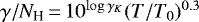 .
.
All Tables
Stellar parameters for selected Gaia FGK benchmark stars from Heiter et al. (2015) and Jofré et al. (2014).
Molecular species, recommended dissociation energies D00, and references for molecular transitions.
Transitions for which multiple fine-structure components were merged into one line in the preselected line list.
Lines of Fe II, Na I, Si I, and Ca II with synflag = Y or U, and with gf_flag = U or N.
Abundance statistics (number of lines, mean, and standard deviation of log εX + 12, where εX = NX∕NH) for four species and four Gaia FGK benchmark stars.
HFS constants and isotopic shifts relative to the ground state (4s 2S) for five Cu I levels.
Wavelength shifts for isotopes with baryon numbers 150 and 142 relative to isotope 144 for the 53 preselected Nd II lines.
HFS constants for 34 out of the 69 Nd II levels involved in the preselected transitions.
HFS constants for nine out of the ten Sm II levels involved in the preselected transitions, for isotopes with non-zero nuclear spin.
References for gf-values for species which occur only in the background line list.
Publications of line-broadening data from ABO theory and applicable ranges of effective principal quantum numbers for neutral species.
Ionisation energies Eion of neutral species listed in Tables G.2 and G.3 and ground states of corresponding singly ionised species (Martin et al. 2011; Ralchenko et al. 2011).
Atomic data for high-quality lines of neutral species in the preselected Gaia-ESO line list which are not included in Barklem et al. (2000b).
Effective principal quantum numbers n*, and ABO theory broadening data, for high-quality lines of neutral species, which are not included in Barklem et al. (2000b).
All Figures
|
Fig. 1 Comparison of observed and calculated line profiles around four of the preselected Fe I lines with different gf_flag assignments for the Sun (left) and Arcturus (right). Black lines: observations, red lines: calculations including preselected spectral lines only. All of these lines are flagged with Y with respect to their blending properties. We would like to point out that the gf_flag assignments were based purely on the type of the gf-value sources. Theperformance of the lines in syntheses of the Sun and Arcturus were not taken into account. These are shown here for illustrative purposes only. |
| In the text | |
|
Fig. 2 Observed (black) and calculated (red) spectra for the Sun for an 8 nm-wide interval in the optical region. The Gaia-ESO bulk line list was used as input for the calculations, which includes preselected and background lines. Some of the strongest preselected lines are labelled by their species. |
| In the text | |
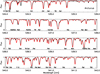 |
Fig. 3 Same as Fig. 2, but for Arcturus. |
| In the text | |
|
Fig. 4 Comparison of observed and calculated line profiles around four of the preselected Fe I lines with different synflag assignments for the Sun (left) and Arcturus (right). Black lines: observations, red lines: calculations including preselected spectral lines only, blue lines: calculations using the Gaia-ESO bulk line list, including preselected and background lines. All of these lines have gf_flag = Y. |
| In the text | |
|
Fig. 5 Line profiles for four preselected Fe I lines generated from observed spectra of selected Gaia FGK benchmark stars (see Sect. 2.3). Quality flags and lower level energy are given at the top of each panel. The vertical dashed line indicates central wavelength. We note that Teff is coded by colour, solid lines are dwarfs, and dotted lines are giants. |
| In the text | |
|
Fig. B.1 Observed spectra of selected Gaia FGK benchmark stars around the Li I 670.8 nm feature (see Sect. 2.3). |
| In the text | |
|
Fig. B.2 Line profiles around the Li I feature for the Sun and Arcturus. Black lines: observations, red lines: calculations including preselected spectral lines only, blue lines: calculations including blends from background line list. For Arcturus the Li abundance was set to log (εLi) +12 = −0.8 dex, where εLi = NLi∕NH (e.g. Brown et al. 1989; Guiglion et al. 2016). |
| In the text | |
|
Fig. B.3 Line-by-line Si I abundances determined for four benchmark stars for two groups of lines with different quality assessment of their transition probabilities, as a function of equivalent width and lower level energy. Abundances are given as log (εSi) + 12, where εSi = NSi∕NH. Only lines with synflag = Y or U and with equivalent widths >5 mÅ are included. |
| In the text | |
|
Fig. B.4 Observed and calculated line profiles around two preselected Ca I lines for the Sun (top row) and Arcturus (middle row). Black lines: observations, red lines: calculations including preselected spectral lines only, blue lines: calculations including blends from background line list. Bottom row: line profiles generated from observed spectra of selected Gaia FGK benchmark stars. See Sect. 2.3. |
| In the text | |
|
Fig. B.5 Observed (black dotted lines) and synthesised (red solid lines) solar spectra of the Ca II near-infrared (NIR) triplet linesat 849.8, 854.2, and 866.2 nm, from top to bottom. The lines are shifted with respect to their central wavelength and offsets are added to the normalised fluxes for clarity. |
| In the text | |
|
Fig. B.6 Observed and calculated line profiles around two preselected Sc II lines for the Sun (top row) and Arcturus (middle row). Black lines: observations, red lines: calculations including preselected spectral lines only, blue lines: calculations including blends from background line list. Bottom row: line profiles generated from observed spectra of selected Gaia FGK benchmark stars. See Sect. 2.3. |
| In the text | |
|
Fig. B.7 Observed and calculated line profiles around two preselected Ti I and Ti II lines for the Sun (top row) and Arcturus (middle row). Black lines: observations, red lines: calculations including preselected spectral lines only, blue lines: calculations including blends from background line list. Bottom row: line profiles generated from observed spectra of selected Gaia FGK benchmark stars. See Sect. 2.3. |
| In the text | |
|
Fig. B.8 Observed and calculated line profiles around preselected lines of V I (left) and Co I (right) for the Sun (top) and Arcturus (middle). Black lines: observations, red lines: calculations including preselected spectral lines only, blue lines: calculations including blends from background line list. Bottom: line profiles generated from observed spectra of selected Gaia FGK benchmark stars. See Sect. 2.3. |
| In the text | |
|
Fig. B.9 Line-by-line Cr I abundances determined for four benchmark stars for two groups of lines with different quality assessment of their transition probabilities, as a function of equivalent width and lower level energy. Abundances are given as log (εCr) + 12, where εCr = NCr∕NH. Only lines with synflag = Y or U and with equivalent widths >5 mÅ are included. |
| In the text | |
|
Fig. B.10 Observed and calculated line profiles around two preselected Mn I lines for the Sun (top row) and Arcturus (middle row). Black lines: observations, red lines: calculations including preselected spectral lines only, blue lines: calculations including blends from background line list. Bottom row: line profiles generated from observed spectra of selected Gaia FGK benchmark stars. See Sect. 2.3. |
| In the text | |
|
Fig. B.11 Comparison of Fe I transition probabilities published by May et al. (1974) to newer, more accurate data from the Oxford, Madison, Hannover, and London groups (see text for references). The solid line indicates the proposed normalisation of the May et al. (1974) values by Fuhr et al. (1988). Applying this normalisation would shift the zero-point on the vertical axis to the solid line (while the data points would remain at the same positions relative to the solid line). All published spectral lines in the wavelength region 476 to 895 nm are shown. |
| In the text | |
|
Fig. B.12 Line-by-line Fe I abundances determined for four benchmark stars for three groups of lines with different quality assessment of their transition probabilities, as a function of equivalent width and lower level energy. Abundances are given as log (εFe) + 12, where εFe = NFe∕NH. Only lines with synflag = Y or U and with equivalent widths >5 mÅ are included. |
| In the text | |
|
Fig. B.13 Line-by-line Ni I abundances determined for four benchmark stars for three groups of lines with different quality assessment of their transition probabilities, as a function of equivalent width and lower level energy. Abundances are given as log (εNi) + 12, where εNi = NNi∕NH. Only lines with synflag = Y or U and with equivalent widths >5 mÅ are included. |
| In the text | |
|
Fig. B.14 Line profiles for two high-quality preselected Zr I lines, which are weak in solar-type stars but strong in cooler stars. Generated from observed spectra of selected Gaia FGK benchmark stars. See Sect. 2.3. |
| In the text | |
|
Fig. B.15 Line profiles for high-quality preselected Mo I lines generated from observed spectra of selected Gaia FGK benchmark stars. See Sect. 2.3. |
| In the text | |
|
Fig. B.16 Line profiles for preselected Ba II lines generated from observed spectra of selected Gaia FGK benchmark stars. See Sect. 2.3. |
| In the text | |
|
Fig. B.17 Comparison between theoretical (the) and experimental (exp) transition probabilities Aul for La II. Data are from Kułaga-Egger & Migdałek (2009) and Lawler et al. (2001a), respectively. The blue vertical line indicates the location of the line at 593.6 nm. |
| In the text | |
|
Fig. B.18 Comparison of observed and calculated line profiles around the two La II lines at 492.2 nm (upper panels, gf_flag = Y, synflag = N), and at 593.6 nm (lower panels, gf_flag = U, synflag = Y) for the Sun (left) and Arcturus (right). Black lines: observations, red lines: calculations including preselected spectral lines only, blue lines: calculations including blends from background line list. |
| In the text | |
|
Fig. B.19 Line profiles for preselected La II lines generated from observed spectra of selected Gaia FGK benchmark stars. See Sect. 2.3. |
| In the text | |
|
Fig. B.20 Line profiles for preselected Ce II lines generated from observed spectra of selected Gaia FGK benchmark stars. See Sect. 2.3. |
| In the text | |
|
Fig. B.21 Observed and calculated line profiles around two preselected Pr II lines for the Sun (top row) and Arcturus (middle row). Black lines: observations, red lines: calculations including preselected spectral lines only, blue lines: calculations including blends from background line list. Bottom row: line profiles generated from observed spectra of selected Gaia FGK benchmark stars. See Sect. 2.3. |
| In the text | |
|
Fig. B.22 Comparison between calibrated (cal) and experimental (exp) transition probabilities for Nd II lines in the UVES-580 wavelength range. The data are from Kurucz & Bell (1995) based on Meggers et al. (1975) and from Den Hartog et al. (2003), respectively. The solid black line indicates the mean difference in loggf, and the dashed lines indicate the standard deviation. |
| In the text | |
|
Fig. B.23 Comparison of observed and calculated line profiles around four of the preselected Nd II lines for the Sun (left) and Arcturus (right). Black lines: observations, red lines: calculations including preselected spectral lines only, blue lines: calculations including blends from background line list. |
| In the text | |
|
Fig. B.24 Line profiles for preselected Nd II lines generated from observed spectra of selected Gaia FGK benchmark stars. See Sect. 2.3. |
| In the text | |
|
Fig. B.25 Observed and calculated line profiles around two preselected Sm II lines for the Sun (top row) and Arcturus (middle row). Black lines: observations, red lines: calculations including preselected spectral lines only, blue lines: calculations including blends from background line list. Bottom row: line profiles generated from observed spectra of selected Gaia FGK benchmark stars. See Sect. 2.3. |
| In the text | |
|
Fig. B.26 Observed and calculated line profiles around two preselected Eu II lines for the Sun (top row) and Arcturus (middle row). Black lines: observations, red lines: calculations including preselected spectral lines only, blue lines: calculations including blends from background line list. Bottom row: line profiles generated from observed spectra of selected Gaia FGK benchmark stars. See Sect. 2.3. |
| In the text | |
|
Fig. B.27 Observed and calculated line profiles around the preselected Gd II and Dy II lines for the Sun (top row) and Arcturus (middle row). Black lines: observations, red lines: calculations including preselected spectral lines only, blue lines: calculations including blends from background line list. Bottom row: line profiles generated from observed spectra of selected Gaia FGK benchmark stars. See Sect. 2.3. |
| In the text | |
|
Fig. F.1 Ratio of collisional line width γ calculated from ABO theory to line width from van der Waals theory using Kurucz or Unsöld C6 values, for Fe I lines of transition types s–p, p–s, and p–d, at a temperature of 6000 K, as a function of lower level energy Elow. |
| In the text | |
|
Fig. F.2 Ratio of collisional line width γ calculated from ABO theory to line width from van der Waals theory using Kurucz or Unsöld C6 values, for Fe II lines of transition types s–p, p–s, p–d (upper panel), d–p and p–p (lower panel), at a temperature of 6000 K, as a function of lower level energy Elow. |
| In the text | |
Current usage metrics show cumulative count of Article Views (full-text article views including HTML views, PDF and ePub downloads, according to the available data) and Abstracts Views on Vision4Press platform.
Data correspond to usage on the plateform after 2015. The current usage metrics is available 48-96 hours after online publication and is updated daily on week days.
Initial download of the metrics may take a while.