| Issue |
A&A
Volume 693, January 2025
|
|
|---|---|---|
| Article Number | A294 | |
| Number of page(s) | 15 | |
| Section | Galactic structure, stellar clusters and populations | |
| DOI | https://doi.org/10.1051/0004-6361/202452537 | |
| Published online | 24 January 2025 | |
Chemical Evolution of R-process Elements in Stars (CERES)
IV. An observational run-up of the third r-process peak with Hf, Os, Ir, and Pt
1
Institute for Applied Physics, Goethe University Frankfurt,
Max-von-Laue-Str. 12,
Frankfurt am Main
60438,
Germany
2
Institut für Kernphysik, Technische Universität Darmstadt,
64289
Darmstadt,
Germany
3
Helmholtz-Institut Jena,
Fröbelstieg 3,
07743
Jena,
Germany
4
GSI Helmholtzzentrum für Schwerionenforschung GmbH,
64291
Darmstadt,
Germany
5
Max-Planck-Institut für Kernphysik,
Saupfercheckweg 1,
Heidelberg
69117,
Germany
6
Departament d’Astronomia i Astrofísica, Universitat de València, Edifici d’Investigació Jeroni Munyoz,
C/ Dr. Moliner, 50,
46100
Burjassot, València,
Spain
7
GEPI, Observatoire de Paris, Université PSL, CNRS,
5 place Jules Janssen,
92195
Meudon,
France
8
Institute for Theoretical Physics, Friedrich-Schiller-University Jena,
07743
Jena,
Germany
★ Corresponding author; This email address is being protected from spambots. You need JavaScript enabled to view it.
Received:
8
October
2024
Accepted:
18
November
2024
Abstract
Context. The third r-process peak (Os, Ir, Pt) is poorly understood due to observational challenges, with spectral lines located in the blue or near-ultraviolet region of stellar spectra. These challenges need to be overcome for a better understanding of the r-process in a broader context.
Aims. To understand how the abundances of the third r-process peak are synthesised and evolve in the Universe, it is necessary to carry out a homogeneous chemical analysis of metal-poor stars using high-quality data observed in the blue region of the electromagnetic spectrum (<400 nm). We provide a homogeneous set of abundances for the third r-process peak (Os, Ir, Pt) and Hf, increasing their availability in the literature by up to one order of magnitude.
Methods. We performed a classical 1D, local thermodynamic equilibrium (LTE) analysis of four elements (Hf, Os, Ir, Pt) using ATLAS model atmospheres to fit synthetic spectra on high signal-to-noise-ratio spectra of 52 red giants observed with UVES/VLT in high resolution (>40,000). Due to the heavy line blending involved, we carefully determined upper limits and uncertainties. The observational results are compared with state-of-the-art nucleosynthesis models.
Results. Our sample displays larger abundances of Ir (Z=77) in comparison to Os (Z=76), both of which have been measured in a few stars in the past. The results also suggest decoupling between the abundances of third r-process peak elements with respect to Eu (a rare earth element) in Eu-poor stars. This seems to contradict a co-production scenario of Eu and the third r-process peak elements Os, Ir, and Pt in the progenitors of these objects. Our results are challenging to explain from a nucleosynthetic point of view: the observationally derived abundances indicate the need for an additional early, primary formation channel (or a non-robust r-process).
Key words: nuclear reactions, nucleosynthesis, abundances / stars: abundances / stars: Population II
© The Authors 2025
 Open Access article, published by EDP Sciences, under the terms of the Creative Commons Attribution License (https://creativecommons.org/licenses/by/4.0), which permits unrestricted use, distribution, and reproduction in any medium, provided the original work is properly cited.
This article is published in open access under the Subscribe to Open model. This email address is being protected from spambots. You need JavaScript enabled to view it. to support open access publication.
1 Introduction
To date, we do not know if the rapid neutron-capture process (r-process) always produces heavy elements in a universal, robust way. The r-process is responsible for forming half of the heavy elements, and therefore understanding its nature is important if we are to accurately determine the various enrichment channels, astrophysical formation sites, and the Galactic chemical evolution of the Milky Way and other galaxies.
Since Burbidge et al. (1957) and Lattimer et al. (1977), both observations and theory have made immense progress; yet open questions on the exact formation site and the physics of the r-process remain. The r-process requires environments with very high neutron densities. In recent decades, the locations proposed to host the r-process have converged to events such as rare magneto-rotational-driven core-collapse supernovae (MRSNe), neutron star–black hole mergers, and binary neutron star mergers (NSMs) (Metzger et al. 2010; Winteler et al. 2012; Barnes et al. 2021; Perego et al. 2021; Arcones & Thielemann 2022; Reichert et al. 2024).
So far, direct observations have corroborated only the NSM scenario, after detection of the r-process in the kilonova AT 2017gfo (Soares-Santos et al. 2017; Watson et al. 2019). This has led authors to wonder how unique and robust the r-process is. A NSM-only scenario is challenged by results based on indirect evidence, that is, the chemical profile of stellar photospheres, which act as the fossil record of the cloud from which they formed (Freeman & Bland-Hawthorn 2002). When very low metallicities are reached ([Fe/H]1 ≲ −2.5), it has been observed that the [Eu/Fe] ratio displays a large scatter (Sneden et al. 2008). This result in particular is a challenge to the single-site scenario, because Eu is thought to be a near-pure r-process element, at least in the Solar System (Simmerer et al. 2004).
Also, when the detailed composition of metal-poor stars is unveiled, it is possible to separate the stars into two groups, one lanthanide-poor and the other lanthanide-rich – even when both patterns display similar abundances of species of the first r-process peak (Hansen et al. 2014b). Such variability contradicts the proposed robustness of the r-process. It could be explained either by an astrophysical site with highly variable conditions or a mixture of at least two different sites. Also, the metal-rich tail of the Milky Way disc shows clear indications of the need for two different formation sites, or at least sites with different delay times, to accurately explain the Eu abundances in the Milky Way disc, and the same conclusion appears to apply to dwarf galaxies (Côté et al. 2019; Molero et al. 2021).
In order to look for clues to solve this problem, it is useful to look at the poorly studied third r-process peak elements (Os, Ir, Pt), and compare their behaviour to that of Eu or other r-process elements between the second and third peak in low-metallicity stars. Data is lacking for these species in the literature (see e.g. Fig. 32 of Kobayashi et al. 2020) due to observational challenges, as their detection relies on efficient blue spectrographs with high resolution and a high signal-to-noise ratio. Their strongest spectral lines are found in the near-ultraviolet, and their observation often requires space-based telescopes. Its increased spectral coverage has meant that the Hubble Space Telescope has been a major contributor to observational work on the r-process (e.g. Sneden et al. 2003; Cowan et al. 2005; Roederer et al. 2010, 2014b, 2022; Barbuy et al. 2011).
The combination of high resolution, high signal-to-noise ratio (S/N), and low metallicity of the Ultraviolet and Visual Echelle Spectrograph (UVES) spectra targeted within the Chemical Evolution of R-process Elements in Stars (CERES) survey allows the selection and analysis of several Os, Ir, and Pt lines. In addition, we have also chosen to analyse Hf, the first post-lanthanide element between the second and third peak (atomic number, Z=72) in order to compare the behaviour of the third r-process peak elements with that of the heavy r-process elements outside the third peak. So far, to our knowledge the only large survey including third r-process peak elements is that of Roederer et al. (2014a), who present 9 abundances and 61 upper limits for Ir I. Here, we aim to expand the number of abundances derived homogeneously for Ir, and also to present homogeneous abundances for the other elements of the third r-process peak Os and Pt. This study is the fourth in the CERES survey, the aim of which is to produce a full chemical profile of a sample of 52 metal-poor stars, focusing on the r-process. The sample was first presented in Lombardo et al. (2022, hereafter Paper I), along with their stellar parameters and abundances from Na to Zr. In Fernandes de Melo et al. (2024, hereafter Paper II), CNO and Li abundances are studied, while in Lombardo et al. (2025, hereafter Paper III), species from Ba to Eu are measured in the CERES sample.
In Sect. 2, we summarise the CERES sample and the work presented in Paper I to derive the model atmospheres. We also explain the details of the procedures followed to fit the synthetic spectra and to separate detections from upper limits, and additionally discuss the careful error analysis carried out in this work. Results are presented in Sect. 3, followed by a discussion from the observational point of view. We also discuss their implications for the current state-of-the-art nucleosynthesis models. We provide some final remarks in Sect. 4.
2 Data and analysis
Our sample, which is fully described in Paper I, consists of 52 metal-poor red giants, with metallicities in the −3.5 < [Fe/H] < −1.7 interval. None of the targets are found to be C-enhanced (Paper II), and their r-process content is very heterogeneous, with A(Eu)2 abundances spanning ≈2 dex (Paper III).
The targets were observed with UVES, mounted at the Very Large Telescope (Dekker et al. 2000). Observations were carried out in November 2019 and March 2020 (ProjectID: 0104.D–0059(A), PI: Hansen). As stated in Paper I, the resolution of these observations is R = λ/Δλ ≳ 40 000, resulting from a configuration using a 1″ slit, 1 × 1 binning, and the standard Dic 1 configuration with blue and red arms centred on 390 and 564 nm. In this configuration, the blue CCD covers a spectral range between 326 and 454 nm.
In addition to the observations, we complement the sample with spectra of similar quality observed with UVES and available in the European Southern Observatory (ESO) archive. The archival spectra span resolutions ranging between 40 000 and 80 000, and a few of these targets have the blue arm centred at 346 nm. For these spectra, the wavelength coverage in the blue CCD spans from 303 to 388 nm. The resulting median signal-to-noise ratio at 390 nm is ≈100 for the whole sample. Further details on the observations are described in Paper I.
2.1 Model atmospheres and chemical abundances
In order to derive abundances of Hf, Os, Ir, and Pt, we used the November 2019 version of MOOG3 (Sneden 1973) to fit synthetic spectra generated with 1D, local thermodynamic equilibrium (LTE), plane-parallel, alpha-enhanced atmospheric models created with the ATLAS12 code (Kurucz 2005). These models were originally calculated for Paper I, and were also employed in Papers II and III to maintain homogeneity.
Stellar parameters used to create atmospheric models are those derived in Paper I, where the iterative procedure adopted is fully described. In summary, effective temperatures Teff and surface gravity values in terms of log g were calculated following the method outlined in Koch-Hansen et al. (2021), which inter-polates Gaia (GBP-GRP) colours in a grid of model atmospheres using the reddening law from Fitzpatrick et al. (2019), the reddening maps from Schlafly & Finkbeiner (2011), and Gaia EDR3 photometry in the G, GBP, and GRP bands (Gaia Collaboration 2016, 2021). Microturbulent velocities vt were calculated using the formula from Mashonkina et al. (2017), and the metallicities are the Fe I abundances giving [Fe/H]. We refer to Paper I for Fe I and Fe II abundances. The adopted uncertainty in [Fe/H] is 0.13 dex, following Paper I.
For a given star, with a given atmospheric model, the abundances A(X) were determined by applying chi-square minimisation between the observed and synthetic spectra for each star. To differentiate abundance detections from upper limits, we developed an empirical method, which we describe in the following section.
Definition of upper limits
Since several lines measured in this work are heavily blended, a careful treatment is necessary for flagging upper limits. After deriving the best-fitting abundance, we used MOOG to synthesise the model of a single isolated spectral line with the atomic parameters of the line being measured (wavelength, lower excitation potential, log gf), as well as that best-fitting abundance. To flag a measurement as a detection instead of an upper limit, we consider the line depth of a single line (that is synthesised alone and isolated from its blends) in a normalised spectrum with its best-fitting abundance to be expected to surpass a 3σ threshold over continuum noise.
To define that threshold, we assume the spectral line to have a Gaussian profile. As such, for a fixed full width at half maximum, the relationship between line depth and the area of the Gaussian (i.e. the theoretical equivalent width) is linear. Hence, the treatment may be done in terms of the equivalent width Wλ. The formula from Cayrel (1988) is adopted here to estimate the uncertainty in Wλ:
![Mathematical equation: $\[\sigma_{W_{\lambda}}=\frac{1.5}{S / N} \sqrt{\Delta \lambda ~\delta \lambda},\]$](/articles/aa/full_html/2025/01/aa52537-24/aa52537-24-eq1.png) (1)
(1)
where Δλ is the full width at half maximum of the spectral line, δλ is the pixel size, and the signal-to-noise ratio per pixel S/N is estimated as the inverse of the root mean square (rms) of the continuum noise near each evaluated spectral line.
From Eq. (1) we can define a value Wλ,min – which corresponds to the 3σ threshold – as three times the uncertainty in Wλ:
![Mathematical equation: $\[W_{\lambda, min } \equiv \frac{4.5}{S / N} \sqrt{\Delta \lambda ~\delta \lambda}.\]$](/articles/aa/full_html/2025/01/aa52537-24/aa52537-24-eq2.png) (2)
(2)
Dividing Eq. (2) by the central wavelength of the spectral line λ and taking the logarithm on both sides, we can write it in terms of the reduced width RW:
![Mathematical equation: $\[R W_{\text {min }} \equiv ~\log~ \frac{W_{\lambda,min}}{\lambda}=~\log~ \left[\frac{4.5}{\lambda~(S / N)} \sqrt{\Delta \lambda ~\delta \lambda}\right].\]$](/articles/aa/full_html/2025/01/aa52537-24/aa52537-24-eq3.png) (3)
(3)
The relationship shown above is valid for unblended lines. If we add a term ϕ to take into account the influence of line blending, the final equation becomes:
![Mathematical equation: $\[R W_{\min }=~\log~ 4.5-~\log~ \lambda-~\log~ S / N+0.5(\log~ \delta \lambda+~\log~ \Delta \lambda)+\phi.\]$](/articles/aa/full_html/2025/01/aa52537-24/aa52537-24-eq4.png) (4)
(4)
Formally, ϕ is the difference in dex between the reduced width of the line of interest evaluated without any blends (RWpure) – which corresponds to the abundance measured with the best fit – and the logarithm of the flux subtracted by that same absorption line when the blends are taken into account:
![Mathematical equation: $\[\phi \equiv R W_{\text {pure }}-~\log \left\{\frac{\int_{0}^{+\infty}[f_{\text {no}}(\lambda^{\prime})-f_{\text {fit}}(\lambda^{\prime})] d \lambda^{\prime}}{\lambda}\right\},\]$](/articles/aa/full_html/2025/01/aa52537-24/aa52537-24-eq5.png) (5)
(5)
in which ffit is the best synthetic spectrum fit, and fno is that best fit with the line of interest removed. The value of ϕ tends to zero when line blending is weak. For absorption lines, the integral in Eq. (5) will always be non-negative. The measurement is flagged as an upper limit in cases where RWpure is lower than RWmin. The values of the parameters ϕ, RWpure, and RWmin for each measurement are listed in the external appendix. An exception was made for three stars whose Ir abundances were flagged manually as upper limits. In these cases, the 3513.480 Å Co I and the 3513.818 Å Fe I lines, which blend with the 3513.640 Å Ir I line under evaluation, had their wings strongly under-fitted, likely resulting in an overestimation of these Ir abundances. These stars are each marked with a single asterisk in Table 4 of the external appendix.
Equation (4) can be rewritten in terms of the effective resolution of the spectral line, Reff = λ/Δλ4:
![Mathematical equation: $\[R W_{\text {min }}=~\log~ 4.5-~\log~ R_{\text {eff }}-~\log~ S / N+0.5(\log~ \delta \lambda-~\log~ \Delta \lambda)+\phi.\]$](/articles/aa/full_html/2025/01/aa52537-24/aa52537-24-eq6.png) (6)
(6)
An application of Eq. (4) (or Eq. (6)) takes advantage of the relationship between reduced width and abundance described by the curve of growth (CoG) theory. The CoG is a function describing the relationship between the column density of a particular species and the equivalent width of the resulting spectral line, taking into account atomic parameters such as excitation potential, oscillator strength, and the partition function, as well as the model atmosphere. Its use allows us to quantify a minimum threshold [X/Fe]min of detectable abundance for a given species in a set of given stellar parameters, with dependence on the quality of the observational data, as exemplified in Fig. 1. Abundances below this threshold may be regarded as upper limits.
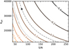 |
Fig. 1 Illustration of the method employed for classification of detections and upper limits. The solid lines are curves of constant [Hf/Fe]min calculated for CES 0031-1647 using Eq. (6) and a CoG model generated with MOOG for the Hf II 3399.8 Å line to convert RWmin to Hf abundances. Their colour scale corresponds to the [Hf/Fe]min labelled in each solid line. The dotted grey line corresponds to the [Hf/Fe] measured in this work, assuming a solar Hf abundance of 0.85 dex (Asplund et al. 2009). The black square marks the point of the estimated S/N and the Reff of CES 0031-1647, indicating that the minimum detectable abundance [Hf/Fe]min for that star with our CERES spectrum is 0.10 dex. The unlabelled dashed line crossing that point represents [Hf/Fe]min = 0.10 for different combinations of S/N and Reff. Abundances to the left of the dashed line will be detections, while abundances to the right side of the dashed line will result in upper limits. |
2.2 Line list
The spectral lines measured in this work are shown in Table 1. The species are Hf II (1 line), Os I (2 lines), Ir I, and Pt I (1 line). These lines are among the strongest spectral lines for these species in the available wavelength range of our spectra, while also being in relatively clean regions devoid of very strong features (e.g. Balmer lines). For the features under consideration, as well as those blending and in the surrounding wavelengths, we employed Linemake5 (Placco et al. 2021) to generate the line lists. The Hf II line has atomic data from Lawler et al. (2007), while for the two Os I features the oscillator strength values are taken from Quinet et al. (2006). The hyperfine and isotopic splitting of the Ir I line comes from Cowan et al. (2005), and uses transition probabilities from Xu et al. (2007). For Pt, atomic data were taken from Hartog et al. (2005). The abundances used to model blends in the spectra surrounding the Hf, Os, and Ir lines were taken from Papers I, II, and III. Isotopic fractions were taken from NUBASE2020 (Meija et al. 2016; Kondev et al. 2021). For 191Ir and 193Ir, they are 0.373 and 0.627, respectively. For the isotopes 192, 194, 195, 196, and 198 of Pt, the corresponding fractions are 0.008, 0.329, 0.338, 0.252, and 0.073. For those lines matching the line list published by Barklem et al. (2000), we adopted constants to model Van der Waals line damping, which were converted from the σABO values listed in Barklem et al. to C6 values using the formula shown in Eq. (A.4) from Coelho et al. (2005). Otherwise, the default UNSLDc6 approximation from Unsold (1955) was calculated by MOOG. Three auxiliary lines in the 3301 Å region had their Linemake log gf values replaced by those available in the Vienna Atomic Line Database (VALD)6 (Piskunov et al. 1995; Brooke et al. 2015; Kurucz 2014, 2016). The VALD values generate better fits on the wings of the Pti line measured in this study. These lines are also shown in Table 1.
In the particular case of the 3399.79 Å Hf II line, there is a blend with a strong NH line (λ=3399.80 Å, lower excitation potential LEP=0.264 eV, log gf=−1.058) that requires very careful consideration. The log gf value adopted in this study for the 3399.79 Å Hf II line is from the Linemake database, and is the same value as that in the line list compiled by Kurucz & Bell (1995)7. However, it is important to note that the value found for its oscillator strength in VALD (Fernando et al. 2018) is 0.3 dex lower than the NH log gf values from Linemake, which were used as a reference in the measurements of the 3360 Å NH band in Paper II; we therefore adopted these latter values in the 3399 Å region for consistency, as the adopted N abundances come from Paper II as well. The log gf values listed in VALD also differ from Linemake by roughly −0.3 dex for most NH lines in the 3360 Å band. For comparison, the log gf values for the NH band in Spite et al. (2005) were also adopted from the Kurucz line list. Appendix A provides a brief discussion on the theoretical modelling of oscillator strength values for NH lines.
Accurate N measurements are crucial in order to determine accurate Hf abundances using the line chosen in this work. After testing synthetic spectra generated with stellar parameters typical of our sample (Teff=5000 K, log g=2.0, [Fe/H]=−2.5, vt=2.0 km s−1), we found that the equivalent width of the (isolated) NH line is almost four times larger than the equivalent width of the (also isolated) Hf II line in the linear part of the curve of growth for solar [Hf/N]. In the most evolved stars in our sample, the pollution of the surface with dredged-up N may result in the NH line dominating the blend entirely, unless the star also displays a large Hf enhancement. Figure 2 shows an example of the contributions of both species for the 3399.8 Å feature. The top (bottom) panel of Fig. 2 shows a star with a low (high) ϕ value (defined in Eq. (5)), which means there is a weak (strong) contribution from the NH line for the blend with Hf.
Line list and their respective atomic data.
2.3 Uncertainties
The uncertainties on A(X) values were calculated taking into account both the process of line formation – by estimating the sensitivity of these lines to the model atmospheres – and observational uncertainties. For a measurement of A(X), the total uncertainty is composed of the sensitivity of A(X) to the internal uncertainties on the atmosphere models listed in Paper I and the sensitivity of A(X) to uncertainties in neighbouring blends. From the observational part, we take into account the uncertainty in the continuum placement, defined as a function of S/N, as well as the residuals of the fit of the synthetic spectrum on the observed data, weighted by their distance to the central wavelength of the line of interest. Formally, the uncertainty σA(X) for each detection of A(X) is
![Mathematical equation: $\[\sigma_{\mathrm{A}(\mathrm{X})}=\sqrt{\sigma_{\Delta}^{2}+\sigma_{\mathrm{c}}^{2}+\sigma_{\mathrm{f}}^{2}},\]$](/articles/aa/full_html/2025/01/aa52537-24/aa52537-24-eq7.png) (7)
(7)
where ![Mathematical equation: $\[\sigma_{\Delta}^{2}\]$](/articles/aa/full_html/2025/01/aa52537-24/aa52537-24-eq8.png) is the quadrature of the sensitivities of A(X) to the uncertainties on the atmospheric parameters
is the quadrature of the sensitivities of A(X) to the uncertainties on the atmospheric parameters ![Mathematical equation: $\[\overrightarrow{a}\]$](/articles/aa/full_html/2025/01/aa52537-24/aa52537-24-eq9.png) = (Teff, log g, [Fe/H], vt) in a particular star. The sensitivity of the abundances to each atmospheric parameter ai is estimated by measuring the extent to which A(X) changes for a 1σ variation of that atmospheric parameter ai, while keeping the other parameters fixed. The adopted uncertainties on the atmospheric parameters were derived in Paper I and their values are
= (Teff, log g, [Fe/H], vt) in a particular star. The sensitivity of the abundances to each atmospheric parameter ai is estimated by measuring the extent to which A(X) changes for a 1σ variation of that atmospheric parameter ai, while keeping the other parameters fixed. The adopted uncertainties on the atmospheric parameters were derived in Paper I and their values are ![Mathematical equation: $\[\overrightarrow{\sigma_{a}}\]$](/articles/aa/full_html/2025/01/aa52537-24/aa52537-24-eq10.png) = (100 K, 0.04 dex, 0.13 dex, 0.5 km s−1).
= (100 K, 0.04 dex, 0.13 dex, 0.5 km s−1).
The uncertainty in continuum placement σc is the change in A(X) that results from the uncertainty generated by noise in the continuum – the choice of the continuum placement may result in a synthetic line that is shallower or deeper than the true spectral line. We estimated σc as the change in A(X) corresponding to the change in the reduced width ΔRW of the spectral line under measurement, which results from a change Δc in the position of the (normalised) spectral continuum. Based on the line depth of σWλ, calculated with Eq. (1) with typical values of δλ = 0.014 Å and Δλ = 0.1 Å from our spectra, Δc is defined as 0.5(S/N)−1, with S/N measured near the spectral line of interest. Under the assumption that the line has a Gaussian profile, we estimated ΔRW as:
![Mathematical equation: $\[\Delta R W=[2 ~\ln (10) ~l~(S / N)]^{-1},\]$](/articles/aa/full_html/2025/01/aa52537-24/aa52537-24-eq11.png) (8)
(8)
by taking the derivative of RW with respect to the depth of the normalised spectral line l.
To estimate the uncertainty on the fit σf, we applied a weight Wε on the residuals of the fit ε(λ) = |fo(λ) − fs(λ)|, where fo(λ) and fs(λ) are the fluxes of the observed and synthetic spectra in a given wavelength, respectively. The weight,
![Mathematical equation: $\[W_{\epsilon}(\lambda)=~\exp~ \left[-\frac{\left(\lambda-\lambda_{c}\right)^{2}}{2 \sigma^{2}}\right],\]$](/articles/aa/full_html/2025/01/aa52537-24/aa52537-24-eq12.png) (9)
(9)
is intended to discard any bias from residuals far from the core of the line. In the above equation, σ corresponds to the width of the line under evaluation, and λc is its central wavelength. We then fitted a Gaussian in the weighted residuals εW(λ) = ε(λ)Wε(λ), and used the value of the fitted Gaussian at the central wavelength of the spectral line as the total change in the line depth due to uncertainty in the fit. As this work deals with blended lines, we estimated the fraction of the subtracted flux in the absorption line corresponding to the species of interest (Hf, Os, Ir, or Pt) in each star, and from that fraction we calculated the corresponding change in line depth – that is, the total change in line depth multiplied by the fraction of the subtracted flux coming from the species being evaluated – due to the fit uncertainty for each species. This change in line depth was used to estimate the change in abundance σf.
The uncertainties for each measurement, as well as their respective sensitivities and partial uncertainties σc and σf are shown in the external appendix. The uncertainties on the abundance ratios discussed in this work were calculated from the A(X) uncertainties using equations A19 and A20 from McWilliam et al. (1995). When abundance ratios are surrounded by square brackets, solar abundances and their respective uncertainties are from Asplund et al. (2009)8. In such cases, the uncertainties on solar abundances were also added in quadrature when propagating the uncertainties on [A/B].
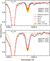 |
Fig. 2 Portion of spectra surrounding the Hf II line at 3399.8 Å for two stars in our sample. Black dots represent the observed spectra. The red solid lines represent the best fit, with their respective [Hf/Fe] shown on the right. Blue dash-dotted lines show synthetic spectra without Hf. Golden dashed lines represent synthetic spectra when N is removed. Grey dotted lines correspond to the synthetic spectra without either N or Hf. Orange shaded areas display a ±0.3 dex interval around the best fit. The N abundances shown are from Paper II. |
3 Results and discussion
The calculated abundances for Hf, Os, Ir, and Pt are shown in Table C.1 along with the stellar parameters from Paper I. Out of our sample of 52 red giants, we were able to derive Hf II abundances for 19 stars, Os I for 33, Ir I for 32, and Pt I for 18 of them. Examples of spectral fitting for the elements of the third r-process peak are shown in Fig. 3. Abundances derived in Papers I, II, and III were used to synthesise the neighbouring lines. For species without abundance information in previous CERES papers, their abundances were assumed to be scaled to solar. For eight of the objects, we were not able to measure abundances for these four species due to insufficient S/N in their spectra and/or glitches in the spectra at the wavelengths of interest. We observed that the extra-mixing that takes place after the red giant branch (RGB) bump does not influence the abundances of these elements. As shown in Fig. 4, apart from the distinction between mixed and unmixed stars around [C/N] ~ 0.5 dex that was used in Paper II as an indicator of extra mixing, we found no evidence that the stars in the upper RGB have an overabundance of Hf, Os, Ir, or Pt with regards to the stars in the lower part of the RGB.
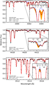 |
Fig. 3 Examples of a spectral fit in Os, Ir, and Pt lines. Black markers show observed spectra. The red solid line indicates the best fit. The blue dash-dotted line shows the spectrum with the species of interest removed. Orange shaded areas are the ±0.3 dex interval around the best fit. Species creating the strongest surrounding lines are labelled in the insets, with the hyperfine–isotopic splitting marked when considered in the line list. The darkest shades of grey indicate the strongest lines. |
3.1 Hafnium
As previously discussed in Sect. 2.1, the strong blend between Hf II and a NH line requires that the N abundances derived in Paper II be considered in the synthesis of the 3399.8 Å line. In Fig. 5 we see that the [Hf/N] ratio negatively correlates with [N/Fe], with Pearson and Spearman correlation coefficients of ρ ≈ −0.7, with p-values of ≈10−4. Figure 5 is colour coded according to surface gravity in order to trace the positions of the stars in the RGB9. The larger concentration of N-rich objects among the stars with upper limits in Hf suggests that the use of the 3399 Å line for Hf measurements is more effective when [N/Fe] ≲ 0.1 dex. Nevertheless, Hf can be detected in some N-rich stars, as indicated by a few measurements in stars with [N/Fe] of greater than 0.4 dex.
Due to the heavy blending between the Hf line and a NH line and the anti-correlation seen in Fig. 5, it is important to verify that the enhancement of NH does not lead to an underestimation of Hf due to the strong blend. A sanity check is to evaluate the distribution of [Hf/Fe], which, in the case of an eventual bias introduced by the NH blend, would be different for N-rich and N-poor stars. We divided our 19 results for [Hf/Fe] into two subsets of [Hf/N]-rich [Hf/N]-poor using the [Hf/N] median of 0.62 dex as the threshold between the two. The two subsets are displayed in Fig. 6, where, upon visual inspection, they do not appear to differ. A two-sample Kolmogorov–Smirnov (KS) test to compare these subsets also does not identify any differences. Using the method stats.ks_2samp from the Python library Scipy (Virtanen et al. 2020) to evaluate the KS statistic, we find a value of 0.38, which is too low to reject the null hypothesis that these two samples could have been drawn from different distributions. Furthermore, when we compare our results with those from Roederer et al. (2014a), which are also shown in Fig. 6, while a difference in the median [Hf/Fe] is clear, the spread in Hf abundances is similar in both studies. The median absolute deviations10 of [Hf/Fe] are 0.4 dex for the CERES sample and 0.5 dex in Roederer et al. (2014a).
In summary, our Hf abundances are not affected by the blend with the NH line, and we attribute the anti-correlation seen in Fig. 5 to the lack of stars with extreme enhancements in Hf, which, if they were to exist, would occupy the upper right area of the plot. In any case, future studies intending to use the 3399.8 Å Hf II line must take N abundances into account for optimisation of the target-selection procedure.
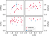 |
Fig. 4 Ratio between [X/Fe] and [C/N] from Paper II. Triangles represent upper limits. Open and filled triangles follow the same classification as the star markers (see the inset in the bottom right-hand panel). |
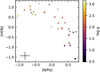 |
Fig. 5 Ratio between Hf and N as a function of the N abundances from Paper II, coloured according to surface gravity. Triangles are upper limits. The error bars in the lower left corner represent the median uncertainties. |
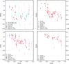 |
Fig. 6 [Hf,Os,Ir,Pt/Fe] versus metallicity [Fe/H], with BD + 173248 (Roederer et al. 2010), CS 22892–052 (Sneden’s star, Sneden et al. 2003), CS 31082–001 (Hill et al. (2002) for Hf, Barbuy et al. (2011) for Os, Ir, Pt), HD 108317 (Roederer et al. 2014b), HD 160617 (Roederer & Lawler 2012), SPLUS J1424–2542 (Placco et al. 2023), and data from Roederer et al. (2012) and Roederer et al. (2014a) for comparison. Arrows are upper limits. The data from Roederer et al. (2014a) also include abundances for CS 22892–052, CS 31082–001, and HD 108317. |
3.2 Osmium
In this work, we derive 33 Os I abundances, plus five upper-limit values. Our results show that Os abundances display enhancement at lower metallicities; see Fig. 6. In the CERES sample, [Os/Fe] shows an anti-correlation with [Fe/H]: their Pearson coefficient is −0.66, with a p-value ≈10−5. This means [Os/Fe] increases with decreasing metallicity, stopping around the metallicity of CS 22892–052 (Sneden et al. 2003, hereafter Sneden’s star). We analyse two lines for this element, located at 3301.565 Å and 4420.468 Å (see Table 1 for their atomic parameters). In stars with measurements of both spectral lines, the bluest line has a median abundance that is 0.11 dex larger than the reddest one, and the median absolute deviation of the line-by-line difference is 0.13 dex. Such a difference between the blue and the red Os I lines has the same magnitude as the effect from Rayleigh scattering found by Reichert et al. (2020) in Sr. The A(Os) = +0.02 adopted by Sneden et al. (2003) for Sneden’s star is from the line at 3301.565 Å. Comparing our abundances with the measurement for Sneden’s star suggests a relative enhancement in Os in the latter. Other measurements available in the literature show an agreement with our [Os/Fe] trend, as seen in Fig. 6. Data on Os abundances have been very scarce in the literature so far, preventing a more comprehensive comparison with previous studies.
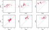 |
Fig. 7 A(X) for each of the four species under study. Markers are the same as in Fig. 6. Dotted lines represent the identity function. Dashed lines represent solar-scaled values; i.e., their y-intercept gives the A(y-axis)/A(x-axis) solar values. Upper limits are omitted in this figure. The x-axis values are the same in all three panels. |
3.3 Iridium
We provide Ir I abundances or upper limits for 38 red giants, of which 32 are detections. Similarly to Os, in Fig. 6 our results show an anti-correlation between [Ir/Fe] and [Fe/H] in the metallicity range of our sample. The Pearson correlation coefficient is −0.68, with a p-value ≈10−5. Interestingly, this anti-correlation fills a gap in the data from Roederer et al. (2014a). In the results of these latter authors, the two stars in the −3 < [Fe/H] < −2 interval are Ir-deficient compared to those in our main anticorrelation pattern. At the same time, our results also present some Ir-deficient stars within the same metallicity range. Sneden et al. (2003) adopted A(Ir) = −0.10 for Sneden’s star. However, that value is an average of two lines: if we consider only their measurement in the same spectral line adopted in this work (3513 Å), the A(Ir) of Sneden’s star increases by 0.05 dex, placing it on the identity function in the bottom panel of Fig. 7, considering the uncertainties. This rescaling makes the result of Sneden et al. (2003) qualitatively similar to one-third of our sample, whose error bars cross the identity function in the A(Ir) versus A(Os) panel in Fig. 7.
3.4 Platinum
Abundances of Pt I are calculated for 18 stars, all of them classified as detections. As in the other two species of the third r-process peak, [Pt/Fe] displays a negative slope against metallicity, albeit milder. In spite of that, the Pearson correlation coefficient between the two quantities is higher, −0.81, with a p-value of ≈10−5, which decreases to −0.89 if the outlier CES 0547–1739 ([Pt/Fe] = 1.49 ± 0.33) is not considered.
Compared to data points available in the literature, our results are consistent with Sneden’s star (Sneden et al. 2003) and CS 31082–001 (Barbuy et al. 2011) in the abundance space shown in Fig. 6. In their reanalysis of CS 31082–001, Ernandes et al. (2023) adopt a value of A(Pt), which is 0.3 dex lower than that found by (Barbuy et al. 2011), but still consistent with the trend found in the CERES sample. Meanwhile, the results for HD 108317 (Roederer et al. 2014b) and HD 160617 (Roederer & Lawler 2012) display a deficiency of Pt compared to our general trend. Apart from Sneden et al. (2003) and Ernandes et al. (2023), all the other works relied on spectral lines below 3000 Å, observed from space with the Hubble Space Telescope. Sneden et al. (2003) used both space- and ground based observations, including the 3301 Å Pt I line adopted in this work. Their Pt abundance for Sneden’s star based on that individual line is 0.06 dex larger than their adopted value, while the log gf adopted by Sneden et al. (2003) is 0.14 dex larger than the log gf used in our measurements. Hence, a more accurate comparison with our results would require a shift of +0.2 dex in the A(Pt) = 0.27 dex abundance adopted by Sneden et al. (2003), assuming that the systematic uncertainties generated by the different model atmospheres employed are negligible. That shift in the Pt abundance would put Sneden’s star in better agreement with our results in Fig. 7.
3.5 Abundance trends
In Figs. 6 and 7, it is clear that the Os, Ir, and Pt abundances exhibit a similar behaviour; they are all anti-correlated with metallicity and show similar slopes in the interval covered by our sample. When compared to Hf, the first post-lanthanide element, they also seem to present the same pattern: a steady increase in A(Os,Ir,Pt) against Hf up to A(Hf) ~ −1.0, followed by an apparent plateau in the more metal-rich stars in Fig. 7. It is not clear whether or not such a plateau exists in Ir versus Hf, because Ir measurements are lacking for stars within the interval of −0.8 < A(Hf) < 0.0 dex. A larger sample in the −2 < [Fe/H] < −1 interval would allow us to verify whether that plateau is real or just a selection effect. Hafnium is the only element analysed in this study with a relatively large share of production by the s-process in the Solar System (49%, Simmerer et al. 2004); therefore, that plateau, if real, may indicate an increase in the s-process contribution to the metal enrichment of that group of stars.
3.5.1 The Eu-poor tail
Figure 8 compares the abundances of the four elements analysed in this work to Eu abundances derived in Paper III, and suggests the existence of a tail in the Eu-poor end for Os, Ir, and Pt The Eu-tails consist of plateaus of the elements from the third r-process peak for stars with A(Eu) ≲ −1.8 dex. These plateaus appear to be roughly centred on A(Os) ~ −0.7, A(Ir) ~ −0.6, and A(Pt) ~ +0.25 dex. The data are coloured by metallicity, and it can be seen that the more metal-rich stars in our sample are absent in the Eu-poor tails, making this a trend that only occurs at the low-metallicity end of our sample. It is interesting to note that the more metal-poor objects, where Os and Ir follow Eu, are r-II stars according to the definition given by Christlieb et al. (2004), which states that r-II stars have [Eu/Fe] > +1.0 and [Ba/Eu] < 0; these are highlighted by red boxes in Fig. 8 Meanwhile, r-I stars are marked by black boxes, while r-poor stars are unmarked. These more metal-poor stars are part of the large spread in Eu that appears in [Fe/H] < −2.5, which has long since been documented in the literature (see e.g. the review from Sneden et al. 2008, and references therein for a discussion).
The results shown in Fig. 8 suggest that the elements in the third r-process peak have a different behaviour with respect to Eu in the [Fe/H] < −2.5 region, despite all four of these species (Eu, Os, Ir, Pt) being nearly pure r-process elements (Simmerer et al. 2004; Bisterzo et al. 2014). In a scenario where these elements are co-produced with Eu, a simple linear relation should appear in their respective panels in Fig. 8. As this linear relation breaks for Eu-poor stars, models must take into account some particular scenarios where elements of the third r-process peak have (relatively) large production rates compared to lanthanides. Interestingly, Hf is the only one among the four elements analysed here that seems to follow Eu, despite being the most s-process-rich species (in the Solar System) studied in this work (by a large margin).
One caveat of our analysis of the behaviour of the third r-process peak elements in relation to Eu is the possibility that yet-to-be-computed metallicity-dependent LTE effects influence Os, Ir, and Pt abundances. However, such corrections should be similar in all three (Os, Ir, Pt) species, making it unlikely that LTE effects are the cause of the Eu-tail. Another caveat is of an observational nature: the existence of a large scatter below the A(Os,Ir) < −1.0 threshold may be currently invisible due to the corresponding spectral lines being too weak. If such star-to-star scatter in third-peak elements exists, S/N values larger than those available in our spectra would be necessary to observe it for Os and Ir. Nevertheless, the lack of scatter of Pt abundances in the Eu-poor region suggests that the Eu-tail must be robust, because the Pt line at 3301 Å is stronger than those lines used for Os and Ir in this work, and the influence of blends in the Pt line is mild to negligible, as indicated by the very low values of ϕ in Table 5 of the external appendix.
Interestingly, a pattern in the Eu abundances with a similar shape and similar metallicity to that from CERES has been noted in the work of Krishnaswamy-Gilroy et al. (1988). In their Fig. 14, these authors compare A(Eu) with an average of A(Sr,Y,Zr), and find a similar trend: the average of A(Sr,Y,Zr) grows mildly in the more Eu-poor stars, and starts to increase more rapidly in the more Eu-rich stars in their sample. The change in slope was attributed to the onset of the s-process. However, in the case of Os, Ir, and Pt, whose s-process contributions in the Solar System are lower than 10% (like Eu), this conclusion is unlikely to hold. Hansen et al. (2014a) also measured a similar trend of Eu with respect to Mo and Ru, which have a large s-process production share in the Solar System compared to the r-process third-peak elements. In that case (i.e. Mo, Ru), the Eutail also forms below A(Eu) ≈ −1.8 dex. In CERES data, we also found a similar tail when comparing the third r-process peak to Ba (see Fig. B.1).
When putting stellar abundances into the context of Galactic chemical evolution, it is important to consider mono-enrichment, which is where a star is formed from a gas previously enriched by a single event of stellar nucleosynthesis. Hartwig et al. (2018) proposed the Mg/C ratio as a tracer for mono-enrichment based on Population III supernova yields. From the [Mg/C] ratios derived in Paper II, no star in our sample at first glance appears mono-enriched. However, this could be due to our sample selection removing carbon-enhanced metal-poor (CEMP) stars from this study, and dilution must also be taken into consideration when comparing models with observations (see Hansen et al. 2020; Magg et al. 2020). Still, the shape observed in Fig. 8, with a transition from a flat third peak to coproduction with Eu around A(Eu) ≈ −1.8, if real, may mean some form of transition in the chemical enrichment of the Universe. In order to look for traces of the s-process in the low metallicity range in which the Eu tail appears, we singled out two members of the metal-poor, Eu-poor tail (CES 1322–1355, CES 1402+0941), as well as two metal-poor, Eu-rich, Os-rich stars (CES 2254–4209, CES 2330–5626), for measurement of Pb. However, the strongest Pb feature in our spectral range, at 4057 Å, is undetectable in the spectra of any of the test targets. An alternative to the measurement of Pb would be to perform measurements of isotopic ratios of Ba to trace the s-process (as in e.g. Magain & Zhao 1993; Mashonkina & Zhao 2006; Gallagher et al. 2010, 2012, 2015; Mashonkina & Belyaev 2019), ideally with a full 3D, non-LTE treatment such as that applied to the Sun by Gallagher et al. (2020). Such a Ba analysis could yield valuable information on the contribution of the s-process, if present, to the enrichment of the interstellar medium before the formation of these stars. However, such an analysis requires much higher S/N values than those available in our sample. If the contribution from the s-process could be ruled out (i.e., if at least some of these stars are r-process pure), modelling of previous enrichment events would be facilitated. In Paper III, the stars with [Ba/Eu] ≤ −0.7 were discussed as being r-pure stars, that is, with no s-process contribution. Interestingly, none of those appear in the Eu-tail in Fig. 8, while one is at the transition zone around A(Eu) ≈ −1.9 dex.
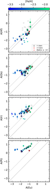 |
Fig. 8 A(Hf,Os,Ir,Pt), from this work, compared to A(Eu) (Paper III). Markers are coloured according to metallicity. Triangles pointing to the left represent upper limits in A(Eu) and detections in the element represented in the y-axis. Triangles pointing down show upper limits for either Hf, Os, or Ir, and detections for Eu. All other markers follow Fig. 6. Lines follow Fig. 7. [Ba/Eu] values are from Paper III. |
3.5.2 Shape of the third r-process peak
The Ir abundances in this work are, on average, 0.18 dex (≈ 1-σ in abundances) larger than Os, with the standard deviation of the difference being 0.17 dex. Hence, our results show that Ir (Z=77) and Os (Z=76) break the even-odd effect in stellar abundances, indicating a monotonic increase in abundances with respect to atomic number from Os to Pt. This increase can be seen in Fig. 9, where we compare CERES data with Sneden’s star and solar-scaled abundances. The monotonic increase in abundances can also be visualised, for instance, in the panels of Fig. 8, with the identity function line crossing the data points in the top panel (Hf vs. Eu), and with the data points moving progressively further away from the identity function in the panels containing Os, Ir, and Pt. This indicates an enhancement of the third peak with respect to Eu.
The lower left panel of Fig. 7 (Ir vs. Os) shows that about one-third of our sample with detections for Ir and Os show a ‘flat’ A(X) versus atomic number profile, that is, their Os and Ir abundances are similar if we take the error bars into account. This is the case, for instance, in the Sun (Asplund et al. 2009; Lodders et al. 2009), in CS 31082–001 (Barbuy et al. 2011), in HD 222925 (Roederer et al. 2018, 2022), and in Sneden’s star (Sneden et al. 2003). On the other hand, HD 160617 (Roederer & Lawler 2012) displays an Ir/Os ratio similar to that of the stars in our sample at the opposite end, that is, those whose Ir abundance is larger than the Os abundance by more than 1σ. Two-thirds of the stars in the CERES sample have significantly larger abundances of Ir than Os. In the case of Pt, if the abundance from Sneden et al. (2003) is shifted by +0.2 dex as discussed in Sect. 3.4, then the A(Pt) from Sneden’s star will differ by less than 1σ from the median A(Pt) shown in Fig. 9.
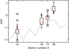 |
Fig. 9 Box plots representing the distributions of A(Hf, Os, Ir, Pt) in our sample. The orange lines represent the medians. The grey dashed line is the solar-scaled abundance normalised to the median of the Os abundances from this work. Open black circles are the outliers in our sample. The filled brown circles are the abundances for Sneden’s star as published by Sneden et al. (2003). |
3.6 Comparison to calculations: New r-process?
In this section, we compare the abundances derived in this work to r-process nucleosynthesis calculations using the nuclear reaction network WinNet (Reichert et al. 2023) and representative trajectories of different r-process sites: neutron star mergers (NSM_R from Rosswog et al. 2013 and NSM_J from Jacobi et al. 2023), their disks (NSM-DISK from Wu et al. 2016), and MRSNe (from Reichert et al. 2021). Figure 10 shows the ratios of Pt/Eu and Os/Eu for the observed abundances and for our calculations. The astrophysical variability is given by the different scenarios (shown with different colours). For each of them, a variety of different nuclear physics inputs is explored (shown with different markers). We have used the FRDM2012 mass model (Möller et al. 2016) and beta decay rates (Möller et al. 2019) together with the fission fragment distributions from Panov et al. (2001) as our default set of nuclear physics inputs. The neutron capture rates were calculated with the Hauser-Feshbach code TALYS and the photodissociation rates are obtained from the principle of detailed balance. For the charged particle reactions, the REACLIB rates are used (Cyburt et al. 2010). In addition, an alternative set of beta-decay rates (D3C*) from Marketin et al. (2016) was explored, as was an alternative set of fission yields, namely beta-delayed and neutron-induced fission fragments from Mumpower et al. (2020) together with spontaneous fission fragments from Kodama & Takahashi (1975). For comparison, the older FRDM1995 mass model (Moller et al. 1995) was also used together with the rates from REACLIB (Cyburt et al. 2010) for all reactions. Finally, two mass models based on energy density functionals were used as described in Martin et al. (2016) and references therein, again with consistent neutron-capture and photodissociation rates: SkM* (Bartel et al. 1982) and UNEDF1 (Kortelainen et al. 2012)11.
Care must be taken when comparing the observed and calculated ratios shown in Fig. 10, because some stars may also contain an s-process contribution, which could increase the Pt/Eu and Os/Eu ratios, as indicated by the values from the solar s-process residuals. In addition, the third r-process peak elements Pt and Os are strongly affected by the nuclear physics inputs, as evidenced by the large scatter. The position of the third peak can be shifted towards heavier elements depending on nuclear masses, beta decays, and neutron-capture cross sections (Arcones & Martínez-Pinedo 2011; Eichler et al. 2015; Mumpower et al. 2015; Marketin et al. 2016; Lund et al. 2023). Furthermore, we use a single representative trajectory per astrophysical model, whereas the mass-weighted sum of multiple tracer particles would solidify our results. Even though the observed stars appear to be multi-enriched (see Sect. 3.5.1), we compare their abundances with calculations of individual nucleosynthesis events. This is justified if the r-process is robust and is therefore produced with the same relative abundances by all scenarios. However, we find a strong enhancement of Os, Ir, and Pt for some stars, corresponding to the third r-process peak. This points to a non-robust or additional r-process. Therefore, the observed abundances could be the outcome of a mixture of different r-process patterns. However, even in such a case, it is not possible to combine the conditions shown in Fig. 10 and reproduce the highest ratios (magenta dots). In order to explain those ratios, one would need at least one scenario with a high production of third-peak elements compared to Eu or Hf and this is not found in any of our conditions. Therefore, the calculated values should be taken with caution. This can be seen by the poor agreement of most calculations with the solar r residuals (solid grey lines) and Sneden’s star (brown dot). However, even if the calculations are inconclusive, some clear trends emerge. One of the models based on MRSN (red in Fig. 10) tends to produce ratios that are too low to explain the majority of stars (black dots). However, the SkM* calculation provides a closer match to the measured values and the conditions cannot be completely ruled out until the nuclear physics is better constrained.
Most stars of this work (black dots in Fig. 10) show comparable Os/Eu ratios to those of the robust r-process patterns, as they are found in the solar r residuals and Sneden’s star. However, the newly observed ratios show a significantly larger scatter. All newly observed Pt/Eu ratios are at least 0.5–1.0 dex larger than those of the robust r-process patterns. This can be interpreted as a deviation of the robustness, or might suggest a systematic bias towards larger Pt abundances in this work.
Three stars exhibit a distinct enhancement of the third r-process peak abundances (magenta dots in Fig. 10). The low metallicities of those stars (see the Eu-tail in Fig. 8) make s-process contributions unlikely; but even the ratios from the solar s residuals (grey dashed lines in Fig. 10) would not be high enough to explain the extreme overabundance of the third-peak elements in these Eu-poor stars. None of our current models for r-process sites can explain the observed abundances of the third peak of these stars, even considering nuclear physics uncertainties. This points to a different r-process pattern compared to solar or Sneden’s star and raises the question of whether or not there is an additional r-process occurring only at low metallicities – that is, at very early times – that produces enhanced abundances of third-peak elements but small Eu abundances. It would be interesting to investigate which astrophysical site could explain such a new r-process.
The discovery of these abundances further supports the variability of the r-process in contrast to a unique robust pattern12 and demonstrates the contribution of an additional r-process at early times. It is puzzling that no currently studied astrophysical environment can fully explain the enhanced Os, Ir, and Pt abundances, even when considering uncertainties in nuclear physics. A potential new r-process may occur under different conditions from those that allow the production of solar r-process and Sneden-like patterns. This highlights the need to compare to observationally derived patterns that are different from those of r-II stars and the Sun. The nuclear physics uncertainties are still very large and our work clearly demonstrates the urgent need to reduce them with experiments and theory. With constrained nuclear physics and additional observational data, the third-peak elements Ir, Os, and Pt will allow direct determination of the astrophysical conditions of a potential new r-process.
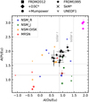 |
Fig. 10 A(Pt/Eu) vs. A(Os/Eu) for observations and nucleosynthesis calculations. Black circles with error bars are abundance detections derived in this work, while left-pointing triangles are upper limits in Os. Sneden’s star is depicted in brown, while the solar r- (s-) residuals are given by the grey solid (dashed) lines. The calculations assume different r-process sites (colours) and different nuclear inputs (symbols). None of the calculations are able to reproduce the large A(Pt/Eu) and A(Os/Eu) values of the three stars in the upper right (magenta), which make up the Eu-tail in Fig. 8. |
4 Final remarks
In this work, we present a homogeneous chemical analysis of 52 stars with high-resolution, high S/N spectra. We have doubled the sample of stellar abundances targeting the third r-process peak (Os, Ir, Pt). We have also demonstrated the viability of carrying out a large, homogeneous analysis of these species using only ground-based spectra. As a result of exploring such relatively uncharted territory, our study has led us to some intriguing conclusions:
The abundances of the elements from the third r-process peak are decoupled from those of Eu for stars with A(Eu) ≲ −1.8 dex. They display a flat trend against A(Eu) before starting to follow Eu. This decoupling is not expected from pairs of elements that are supposed to be co-produced in the same conditions;
In most of the stars studied here, the neighbouring species Os (Z-even) and Ir (Z-odd) significantly break the even–odd pattern seen in stellar abundances. That break has been observed in single stars in previous studies, but here we detect it for a larger, homogeneous sample;
The results discussed in the previous two points highlight the possibility of the existence of some unknown mechanism involving an early r-process. It is unlikely that the s-process has some significant influence in these species (Eu, Os, Ir, Pt), in particular at the metallicity range under analysis here;
Surprisingly, the only element in this study that seems to follow Eu is Hf. The behaviour of Hf in relation to Os, Ir, and Pt may suggest that the more metal-rich end of our sample is already experiencing some s-process enrichment, in agreement with results from Paper III;
This homogeneous study highlights the need for more complete observationally derived abundance patterns at the lowest metallicities (not solar), and the importance of careful treatment of the nucleosynthetic yields and their uncertainties.
Data availability
An external appendix containing five tables is available on Zenodo at https://zenodo.org/records/14225383.
Acknowledgements
We thank the anonymous referee for the comments and suggestions. We would like to thank M. Hanke, M. Eichler, and M. Molero for help with fruitful discussions and data reduction. AAP, JK, CJH, LL, RFM, and AA acknowledge the support by the State of Hesse within the Research Cluster ELEMENTS (Project ID 500/10.006). CJH also acknowledges the European Union’s Horizon 2020 research and innovation programme under grant agreement No 101008324 (ChETEC-INFRA). AA was supported by Deutsche Forschungsgemeinschaft (DFG, German Research Foundation) – Project-ID 279384907 – SFB 1245. MR acknowledges support from the Juan de la Cierva program (FJC2021-046688-I) and the grant PID2021-127495NB-I00, funded by MCIN/AEI/10.13039/501100011033 and by the European Union “NextGenerationEU” as well as “ESF Investing in your future”. Additionally, he acknowledges support from the Astrophysics and High Energy Physics program of the Generalitat Valenciana ASFAE/2022/026 funded by MCIN and the European Union NextGenerationEU (PRTR-C17.I1) as well as support from the Prometeo excellence program grant CIPROM/2022/13 funded by the Generalitat Valenciana. EC and PB acknowledge support from the ERC advanced grant N. 835087 SPIAKID. This work has made use of data from the European Space Agency (ESA) mission Gaia (https://www.cosmos.esa.int/gaia), processed by the Gaia Data Processing and Analysis Consortium (DPAC, https://www.cosmos.esa.int/web/gaia/dpac/consortium). Funding for the DPAC has been provided by national institutions, in particular the institutions participating in the Gaia Multilateral Agreement. This work has made use of the VALD database, operated at Uppsala University, the Institute of Astronomy RAS in Moscow, and the University of Vienna. This work has made use of the Python libraries Numpy (Harris et al. 2020) and Matplotlib (Hunter 2007).
Appendix A Discussion on modelling of NH lines
As an alternative to the discrepant values of oscillator strength found in the literature, as previously discussed in Sect. 2.2, we tried a fully theoretical approach in order to derive self-consistent log gf values for the NH lines of interest in the CERES project. We performed ab initio molecular calculations on the potential energy curves for the electronic ground X 3Σ and A 3Π states of NH over a range of internuclear distances from 0.8 up to 10 Å. All the computations were carried out with the Dyall’s all-electron core-valence correlated basis set with highest angular momentum equal to 4 (dyall.acv4z). The (small) relativistic effects were modelled by means of the eXact-2-component (X2C) (Peng & Reiher 2012) correction to the molecular Hamiltonian. The electronic structure was first modelled with the multi-configuration Dirac-Hartree-Fock method, where six valence electrons were distributed over thirteen active atomic orbitals (N’s 2s, 2p, 3s and 3p; H’s 1s, 2s, 2p). The wavefunctions thus computed were used as a reference for the subsequent Multi-Reference Configuration-Interaction (MRCI) method (Szalay et al. 2011). The active space included all the NH electrons and accounted for single, double and triple valence excitations. All the calculations were performed with the help of the DIRAC23 (Bast et al. 2023) quantum-chemistry software. Rovibronic transitions were obtained by solving the nuclear Schrödinger equation with the help of the software LEVEL (Le Roy 2017).
In Table A.1, we reported the equilibrium distances Re and dissociation energies De for the electronic ground X 3Σ− and first excited A 3Π of NH, alongside the related energies for the first vibrational level E(v = 0). For the electronic ground state, our computed internuclear distance falls between the benchmark values of Fernando et al. (2018) and Melosso et al. (2019), while the dissociation energy is slightly overestimated (4.9%) with respect to the former reference. In contrast, our energy for the first vibrational level lies only 0.3% below the benchmark value of Fernando et al.. The accuracy of our spectroscopic parameters further increases with regards to the first excited state, where the discrepancies between our values for De and E(v = 0) and the results by Fernando et al. amount to 0.95% and 0.47%, respectively.
Equilibrium distance (Re), dissociation energy (De) and energy of the first vibrational level for the electronic ground state X 3Σ− and the first excited state A 3Π of NH.
Energies for transition from a lower rovibronic state (Elow) to an upper rovibronic state (Eup), alongside the related transition wavelengths in air and log gf.
We further checked the compliance of our calculations with the experimental accuracy requirements by estimating three rovibronic transitions involving the X 3Σ− and A 3Π states. Besides the aforementioned electronic states, these transitions encompass the v = 0 vibrational level, and the J = 6, 7, 11 and J = 7, 8, 10 rotational levels embedded within both the electronic states. In Table A.2 we identified these transitions by means of the energy of the lower and upper rovibronic states, the related photon absorption wavelengths in air, and log gf. Our results were compared with the reference data of Fernando et al. (2018). While the discrepancies between the two result sets is overall reasonable (between 2 and 7% on the photon wavelengths in air), they still cannot comply with the 8 Å experimental resolution. These discrepancies might be reduced by improving the modelling of electron correlation within the intrinsic limits of the MRCI method, by inclusion of higher-order electron excitations; account for non-Born-Oppenheimer effects, following the work of Melosso et al. (2019) should also improve the accuracy of the results.
Appendix B Third peak compared to Ba
In Fig. B.1 we show the behaviour of Os against Ba.
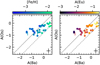 |
Fig. B.1 A(Os) as function of the A(Ba) abundances calculated in Paper III for our sample. Dotted lines represent the identity function. Dashed lines represent solar-scaled values. Arrows are upper limits. The representative error bars correspond to the median uncertainties. |
Appendix C Abundances of Hf, Os, Ir, and Pt
Stellar parameters Teff, log g, and [Fe/H] from Paper I, and the abundances calculated in this work in the A(X) scale.
References
- Arcones, A., & Martínez-Pinedo, G. 2011, Phys. Rev. C, 83, 045809 [CrossRef] [Google Scholar]
- Arcones, A., & Thielemann, F.-K. 2022, A&A Rev., 31, 1 [Google Scholar]
- Asplund, M., Grevesse, N., Sauval, A. J., & Scott, P. 2009, ARA&A, 47, 481 [NASA ADS] [CrossRef] [Google Scholar]
- Barbuy, B., Spite, M., Hill, V., et al. 2011, A&A, 534, A60 [NASA ADS] [CrossRef] [EDP Sciences] [Google Scholar]
- Barklem, P. S., Piskunov, N., & O’Mara, B. J. 2000, A&AS, 142, 467 [NASA ADS] [CrossRef] [EDP Sciences] [Google Scholar]
- Barnes, J., Zhu, Y. L., Lund, K. A., et al. 2021, ApJ, 918, 44 [CrossRef] [Google Scholar]
- Bartel, J., Quentin, P., Brack, M., Guet, C., & Håkansson, H.-B. 1982, Nucl. Phys. A, 386, 79 [CrossRef] [Google Scholar]
- Bast, R., Gomes, A. S. P., Saue, T., et al. 2023, https://doi.org/10.5281/zenodo.7670749 [Google Scholar]
- Bisterzo, S., Travaglio, C., Gallino, R., Wiescher, M., & Käppeler, F. 2014, ApJ, 787, 10 [NASA ADS] [CrossRef] [Google Scholar]
- Brooke, J. S. A., Bernath, P. F., & Western, C. M. 2015, J. Chem. Phys., 143, 026101 [CrossRef] [Google Scholar]
- Burbidge, E. M., Burbidge, G. R., Fowler, W. A., & Hoyle, F. 1957, Rev. Mod. Phys., 29, 547 [NASA ADS] [CrossRef] [Google Scholar]
- Caffau, E., Ludwig, H.-G., Steffen, M., Freytag, B., & Bonifacio, P. 2010, Sol. Phys., 268, 255 [Google Scholar]
- Cayrel, R. 1988, in IAU Symposium, 132, The Impact of Very High S/N Spectroscopy on Stellar Physics, eds. G. Cayrel de Strobel, & M. Spite, 345 [Google Scholar]
- Christlieb, N., Beers, T. C., Barklem, P. S., et al. 2004, A&A, 428, 1027 [NASA ADS] [CrossRef] [EDP Sciences] [Google Scholar]
- Coelho, P., Barbuy, B., Meléndez, J., Schiavon, R. P., & Castilho, B. V. 2005, A&A, 443, 735 [NASA ADS] [CrossRef] [EDP Sciences] [Google Scholar]
- Côté, B., Eichler, M., Arcones, A., et al. 2019, ApJ, 875, 106 [Google Scholar]
- Cowan, J. J., Sneden, C., Beers, T. C., et al. 2005, ApJ, 627, 238 [NASA ADS] [CrossRef] [Google Scholar]
- Cyburt, R. H., Amthor, A. M., Ferguson, R., et al. 2010, ApJS, 189, 240 [NASA ADS] [CrossRef] [Google Scholar]
- Dekker, H., D’Odorico, S., Kaufer, A., Delabre, B., & Kotzlowski, H. 2000, Proc. SPIE, 4008, 534 [Google Scholar]
- Eichler, M., Arcones, A., Kelic, A., et al. 2015, ApJ, 808, 30 [NASA ADS] [CrossRef] [Google Scholar]
- Ernandes, H., Castro, M. J., Barbuy, B., et al. 2023, MNRAS, 524, 656 [NASA ADS] [CrossRef] [Google Scholar]
- Fernandes de Melo, R., Lombardo, L., Alencastro Puls, A., et al. 2024, A&A, 691, A220 [NASA ADS] [CrossRef] [EDP Sciences] [Google Scholar]
- Fernando, A. M., Bernath, P. F., Hodges, J. N., & Masseron, T. 2018, J. Quant. Spec. Radiat. Transf., 217, 29 [NASA ADS] [CrossRef] [Google Scholar]
- Fitzpatrick, E. L., Massa, D., Gordon, K. D., Bohlin, R., & Clayton, G. C. 2019, ApJ, 886, 108 [Google Scholar]
- Freeman, K., & Bland-Hawthorn, J. 2002, ARA&A, 40, 487 [Google Scholar]
- Gaia Collaboration (Brown, A. G. A., et al.) 2016, A&A, 595, A2 [NASA ADS] [CrossRef] [EDP Sciences] [Google Scholar]
- Gaia Collaboration (Brown, A. G. A., et al.) 2021, A&A, 649, A1 [NASA ADS] [CrossRef] [EDP Sciences] [Google Scholar]
- Gallagher, A. J., Ryan, S. G., García Pérez, A. E., & Aoki, W. 2010, A&A, 523, A24 [NASA ADS] [CrossRef] [EDP Sciences] [Google Scholar]
- Gallagher, A. J., Ryan, S. G., Hosford, A., et al. 2012, A&A, 538, A118 [NASA ADS] [CrossRef] [EDP Sciences] [Google Scholar]
- Gallagher, A. J., Ludwig, H.-G., Ryan, S. G., & Aoki, W. 2015, A&A, 579, A94 [NASA ADS] [CrossRef] [EDP Sciences] [Google Scholar]
- Gallagher, A. J., Bergemann, M., Collet, R., et al. 2020, A&A, 634, A55 [NASA ADS] [CrossRef] [EDP Sciences] [Google Scholar]
- Hansen, C. J., Andersen, A. C., & Christlieb, N. 2014a, A&A, 568, A47 [NASA ADS] [CrossRef] [EDP Sciences] [Google Scholar]
- Hansen, C. J., Montes, F., & Arcones, A. 2014b, ApJ, 797, 123 [NASA ADS] [CrossRef] [Google Scholar]
- Hansen, C. J., Koch, A., Mashonkina, L., et al. 2020, A&A, 643, A49 [NASA ADS] [CrossRef] [EDP Sciences] [Google Scholar]
- Harris, C. R., Millman, K. J., van der Walt, S. J., et al. 2020, Nature, 585, 357 [NASA ADS] [CrossRef] [Google Scholar]
- Hartog, E. A. D., Herd, M. T., Lawler, J. E., et al. 2005, ApJ, 619, 639 [NASA ADS] [CrossRef] [Google Scholar]
- Hartwig, T., Yoshida, N., Magg, M., et al. 2018, MNRAS, 478, 1795 [CrossRef] [Google Scholar]
- Hill, V., Plez, B., Cayrel, R., et al. 2002, A&A, 387, 560 [CrossRef] [EDP Sciences] [Google Scholar]
- Holmbeck, E. M., Frebel, A., McLaughlin, G. C., et al. 2019, ApJ, 881, 5 [NASA ADS] [CrossRef] [Google Scholar]
- Hunter, J. D. 2007, Comput. Sci. Eng., 9, 90 [NASA ADS] [CrossRef] [Google Scholar]
- Jacobi, M., Guercilena, F. M., Huth, S., et al. 2023, MNRAS, 527, 8812 [NASA ADS] [CrossRef] [Google Scholar]
- Kobayashi, C., Karakas, A. I., & Lugaro, M. 2020, ApJ, 900, 179 [Google Scholar]
- Koch-Hansen, A. J., Hansen, C. J., Lombardo, L., et al. 2021, A&A, 645, A64 [NASA ADS] [CrossRef] [EDP Sciences] [Google Scholar]
- Kodama, T., & Takahashi, K. 1975, Nucl. Phys. A, 239, 489 [Google Scholar]
- Kondev, F., Wang, M., Huang, W., Naimi, S., & Audi, G. 2021, Chin. Phys. C, 45, 030001 [NASA ADS] [CrossRef] [Google Scholar]
- Koput, J. 2015, J. Computat. Chem., 36, 1286 [Google Scholar]
- Kortelainen, M., McDonnell, J., Nazarewicz, W., et al. 2012, Phys. Rev. C, 85, 024304 [CrossRef] [Google Scholar]
- Krishnaswamy-Gilroy, K., Sneden, C., Pilachowski, C. A., & Cowan, J. J. 1988 ApJ, 327, 298 [NASA ADS] [CrossRef] [Google Scholar]
- Kurucz, R. L. 2005, Mem. Soc. Astron. Ital. Suppl., 8, 14 [Google Scholar]
- Kurucz, R. L. 2014, Robert L. Kurucz on-line database of observed and predicted atomic transitions, http://kurucz.harvard.edu/atoms/ [Google Scholar]
- Kurucz, R. L. 2016, Robert L. Kurucz on-line database of observed and predicted atomic transitions, http://kurucz.harvard.edu/atoms/ [Google Scholar]
- Kurucz, R. L., & Bell, B. 1995, Atomic line list (Kurucz CD-ROM, Cambridge, MA: Smithsonian Astrophysical Observatory) [Google Scholar]
- Lattimer, J. M., Mackie, F., Ravenhall, D. G., & Schramm, D. N. 1977, ApJ, 213, 225 [NASA ADS] [CrossRef] [Google Scholar]
- Lawler, J. E., Hartog, E. A. D., Labby, Z. E., et al. 2007, ApJS, 169, 120 [NASA ADS] [CrossRef] [Google Scholar]
- Le Roy, R. J. 2017, J. Quant. Spec. Radiat. Transf., 186, 167 [Google Scholar]
- Lodders, K., Palme, H., & Gail, H.-P. 2009, arXiv e-prints [arXiv:0901.1149] [Google Scholar]
- Lombardo, L., Bonifacio, P., François, P., et al. 2022, A&A, 665, A10 [NASA ADS] [CrossRef] [EDP Sciences] [Google Scholar]
- Lombardo, L., Hansen, C. J., Rizzuti, F., et al. 2025, A&A, 693, A293 [NASA ADS] [CrossRef] [EDP Sciences] [Google Scholar]
- Lund, K. A., Engel, J., McLaughlin, G. C., et al. 2023, ApJ, 944, 144 [NASA ADS] [CrossRef] [Google Scholar]
- Magain, P., & Zhao, G. 1993, A&A, 268, L27 [NASA ADS] [Google Scholar]
- Magg, M., Nordlander, T., Glover, S. C. O., et al. 2020, MNRAS, 498, 3703 [Google Scholar]
- Malicet, J., Brion, J., & Guenebaut, H. 1970, J. Chim. Phys., 67, 25 [Google Scholar]
- Marketin, T., Huther, L., & Martínez-Pinedo, G. 2016, Phys. Rev. C, 93, 025805 [CrossRef] [Google Scholar]
- Martin, D., Arcones, A., Nazarewicz, W., & Olsen, E. 2016, Phys. Rev. Lett., 116, 121101 [Google Scholar]
- Mashonkina, L. I., & Belyaev, A. K. 2019, Astron. Lett., 45, 341 [NASA ADS] [CrossRef] [Google Scholar]
- Mashonkina, L., & Zhao, G. 2006, A&A, 456, 313 [NASA ADS] [CrossRef] [EDP Sciences] [Google Scholar]
- Mashonkina, L., Jablonka, P., Pakhomov, Y., Sitnova, T., & North, P. 2017, A&A, 604, A129 [NASA ADS] [CrossRef] [EDP Sciences] [Google Scholar]
- McWilliam, A., Preston, G. W., Sneden, C., & Searle, L. 1995, AJ, 109, 2757 [Google Scholar]
- Meija, J., Coplen, T. B., Berglund, M., et al. 2016, Pure Appl. Chem., 88, 293 [Google Scholar]
- Melosso, M., Bizzocchi, L., Tamassia, F., et al. 2019, PCCP, 21, 3564 [NASA ADS] [CrossRef] [Google Scholar]
- Metzger, B. D., Martínez-Pinedo, G., Darbha, S., et al. 2010, MNRAS, 406, 2650 [NASA ADS] [CrossRef] [Google Scholar]
- Molero, M., Romano, D., Reichert, M., et al. 2021, MNRAS, 505, 2913 [NASA ADS] [CrossRef] [Google Scholar]
- Moller, P., Nix, J., Myers, W., & Swiatecki, W. 1995, At. Data Nucl. Data Tables, 59, 185 [CrossRef] [Google Scholar]
- Möller, P., Sierk, A., Ichikawa, T., & Sagawa, H. 2016, At. Data Nucl. Data Tables, 109, 1 [CrossRef] [Google Scholar]
- Möller, P., Mumpower, M., Kawano, T., & Myers, W. 2019, At. Data Nucl. Data Tables, 125, 1 [CrossRef] [Google Scholar]
- Mumpower, M. R., Surman, R., Fang, D.-L., et al. 2015, Phys. Rev. C, 92, 035807 [Google Scholar]
- Mumpower, M. R., Jaffke, P., Verriere, M., & Randrup, J. 2020, Phys. Rev. C, 101, 054607 [CrossRef] [Google Scholar]
- Owono Owono, L. C., Jaidane, N., Kwato Njock, M. G., & Ben Lakhdar, Z. 2007, J. Chem. Phys., 126, 244302 [Google Scholar]
- Panov, I., Freiburghaus, C., & Thielemann, F.-K. 2001, Nucl. Phys. A, 688, 587 [Google Scholar]
- Peng, D., & Reiher, M. 2012, Theoretical Chemistry Accounts, 131 [Google Scholar]
- Perego, A., Thielemann, F. K., & Cescutti, G. 2021, r-Process Nucleosynthesis from Compact Binary Mergers (Springer Singapore), 1 [Google Scholar]
- Piskunov, N. E., Kupka, F., Ryabchikova, T. A., Weiss, W. W., & Jeffery, C. S. 1995, A&AS, 112, 525 [Google Scholar]
- Placco, V. M., Sneden, C., Roederer, I. U., et al. 2021, RNAAS, 5, 92 [NASA ADS] [Google Scholar]
- Placco, V. M., Almeida-Fernandes, F., Holmbeck, E. M., et al. 2023, ApJ, 959, 60 [NASA ADS] [CrossRef] [Google Scholar]
- Quinet, P., Palmeri, P., Biémont, É., et al. 2006, A&A, 448, 1207 [NASA ADS] [CrossRef] [EDP Sciences] [Google Scholar]
- Reichert, M., Hansen, C. J., Hanke, M., et al. 2020, A&A, 641, A127 [NASA ADS] [CrossRef] [EDP Sciences] [Google Scholar]
- Reichert, M., Obergaulinger, M., Eichler, M., Aloy, M. A., & Arcones, A. 2021, MNRAS, 501, 5733 [NASA ADS] [Google Scholar]
- Reichert, M., Winteler, C., Korobkin, O., et al. 2023, ApJS, 268, 66 [NASA ADS] [CrossRef] [Google Scholar]
- Reichert, M., Bugli, M., Guilet, J., et al. 2024, MNRAS, 529, 3197 [NASA ADS] [CrossRef] [Google Scholar]
- Roederer, I. U., & Lawler, J. E. 2012, ApJ, 750, 76 [NASA ADS] [CrossRef] [Google Scholar]
- Roederer, I. U., Sneden, C., Lawler, J. E., & Cowan, J. J. 2010, ApJ, 714, L123 [NASA ADS] [CrossRef] [Google Scholar]
- Roederer, I. U., Lawler, J. E., Sobeck, J. S., et al. 2012, ApJS, 203, 27 [NASA ADS] [CrossRef] [Google Scholar]
- Roederer, I. U., Preston, G. W., Thompson, I. B., et al. 2014a, AJ, 147, 136 [Google Scholar]
- Roederer, I. U., Schatz, H., Lawler, J. E., et al. 2014b, ApJ, 791, 32 [NASA ADS] [CrossRef] [Google Scholar]
- Roederer, I. U., Sakari, C. M., Placco, V. M., et al. 2018, ApJ, 865, 129 [NASA ADS] [CrossRef] [Google Scholar]
- Roederer, I. U., Lawler, J. E., Den Hartog, E. A., et al. 2022, ApJS, 260, 27 [NASA ADS] [CrossRef] [Google Scholar]
- Rosswog, S., Piran, T., & Nakar, E. 2013, MNRAS, 430, 2585 [NASA ADS] [CrossRef] [Google Scholar]
- Schlafly, E. F., & Finkbeiner, D. P. 2011, ApJ, 737, 103 [Google Scholar]
- Simmerer, J., Sneden, C., Cowan, J. J., et al. 2004, ApJ, 617, 1091 [Google Scholar]
- Sneden, C. A. 1973, PhD thesis, The University of Texas at Austin, USA [Google Scholar]
- Sneden, C., Cowan, J. J., Lawler, J. E., et al. 2003, ApJ, 591, 936 [NASA ADS] [CrossRef] [Google Scholar]
- Sneden, C., Cowan, J. J., & Gallino, R. 2008, ARA&A, 46, 241 [Google Scholar]
- Soares-Santos, M., Holz, D. E., Annis, J., et al. 2017, ApJ, 848, L16 [CrossRef] [Google Scholar]
- Spite, M., Cayrel, R., Plez, B., et al. 2005, A&A, 430, 655 [NASA ADS] [CrossRef] [EDP Sciences] [Google Scholar]
- Szalay, P. G., Müller, T., Gidofalvi, G., Lischka, H., & Shepard, R. 2011, Chem. Rev., 112, 108 [Google Scholar]
- Unsold, A. 1955, Physik der Sternatmospharen, MIT besonderer Berucksichtigung der Sonne (Berlin: Springer) [Google Scholar]
- Virtanen, P., Gommers, R., Oliphant, T. E., et al. 2020, Nature Methods, 17, 261 [CrossRef] [Google Scholar]
- Watson, D., Hansen, C. J., Selsing, J., et al. 2019, Nature, 574, 497 [NASA ADS] [CrossRef] [Google Scholar]
- Winteler, C., Käppeli, R., Perego, A., et al. 2012, ApJ, 750, L22 [Google Scholar]
- Wu, M.-R., Fernández, R., Martínez-Pinedo, G., & Metzger, B. D. 2016, MNRAS, 463, 2323 [NASA ADS] [CrossRef] [Google Scholar]
- Xu, H., Svanberg, S., Quinet, P., Palmeri, P., & Biémont, É. 2007, J. Quant. Spec. Radiat. Transf., 104, 52 [Google Scholar]
![Mathematical equation: $\[[\mathrm{A} / \mathrm{B}]=~\log~ \frac{N_{A} N_{B, \odot}}{N_{B} N_{A, \odot}}\]$](/articles/aa/full_html/2025/01/aa52537-24/aa52537-24-eq13.png) , where Ni is the column density of species i.
, where Ni is the column density of species i.
![Mathematical equation: $\[A(X)=~\log~ \frac{N_{X}}{N_{H}}+12\]$](/articles/aa/full_html/2025/01/aa52537-24/aa52537-24-eq14.png) . That quantity is also referred in the literature as log ε (X).
. That quantity is also referred in the literature as log ε (X).
In the definition of Reff, all line broadening effects are taken into account in Δλ. That is, Δλ is the observed resolution element.
Except the solar abundance of Fe [A(Fe)⊙ = 7.52], which, as in Paper I, comes from Caffau et al. (2010).
Except for CES 2250–4057, which is assumed to be a horizontal branch star; see Paper II.
In this work, the scale factor of the median absolute deviation is adjusted for a normal distribution.
The mass models SkP, SLy4, SV-min, and UNEDF0 were also tested. They result in similar ratios to the ones in Fig. 10 but are left out for visual clarity.
The non-robustness of the r-process has been discussed before concerning the first r-process peak, low abundances after the second peak (Hansen et al. 2014b, and references therein), and Ac-boost stars (Eichler et al. 2015; Holmbeck et al. 2019).
All Tables
Equilibrium distance (Re), dissociation energy (De) and energy of the first vibrational level for the electronic ground state X 3Σ− and the first excited state A 3Π of NH.
Energies for transition from a lower rovibronic state (Elow) to an upper rovibronic state (Eup), alongside the related transition wavelengths in air and log gf.
Stellar parameters Teff, log g, and [Fe/H] from Paper I, and the abundances calculated in this work in the A(X) scale.
All Figures
|
Fig. 1 Illustration of the method employed for classification of detections and upper limits. The solid lines are curves of constant [Hf/Fe]min calculated for CES 0031-1647 using Eq. (6) and a CoG model generated with MOOG for the Hf II 3399.8 Å line to convert RWmin to Hf abundances. Their colour scale corresponds to the [Hf/Fe]min labelled in each solid line. The dotted grey line corresponds to the [Hf/Fe] measured in this work, assuming a solar Hf abundance of 0.85 dex (Asplund et al. 2009). The black square marks the point of the estimated S/N and the Reff of CES 0031-1647, indicating that the minimum detectable abundance [Hf/Fe]min for that star with our CERES spectrum is 0.10 dex. The unlabelled dashed line crossing that point represents [Hf/Fe]min = 0.10 for different combinations of S/N and Reff. Abundances to the left of the dashed line will be detections, while abundances to the right side of the dashed line will result in upper limits. |
| In the text | |
|
Fig. 2 Portion of spectra surrounding the Hf II line at 3399.8 Å for two stars in our sample. Black dots represent the observed spectra. The red solid lines represent the best fit, with their respective [Hf/Fe] shown on the right. Blue dash-dotted lines show synthetic spectra without Hf. Golden dashed lines represent synthetic spectra when N is removed. Grey dotted lines correspond to the synthetic spectra without either N or Hf. Orange shaded areas display a ±0.3 dex interval around the best fit. The N abundances shown are from Paper II. |
| In the text | |
|
Fig. 3 Examples of a spectral fit in Os, Ir, and Pt lines. Black markers show observed spectra. The red solid line indicates the best fit. The blue dash-dotted line shows the spectrum with the species of interest removed. Orange shaded areas are the ±0.3 dex interval around the best fit. Species creating the strongest surrounding lines are labelled in the insets, with the hyperfine–isotopic splitting marked when considered in the line list. The darkest shades of grey indicate the strongest lines. |
| In the text | |
|
Fig. 4 Ratio between [X/Fe] and [C/N] from Paper II. Triangles represent upper limits. Open and filled triangles follow the same classification as the star markers (see the inset in the bottom right-hand panel). |
| In the text | |
|
Fig. 5 Ratio between Hf and N as a function of the N abundances from Paper II, coloured according to surface gravity. Triangles are upper limits. The error bars in the lower left corner represent the median uncertainties. |
| In the text | |
|
Fig. 6 [Hf,Os,Ir,Pt/Fe] versus metallicity [Fe/H], with BD + 173248 (Roederer et al. 2010), CS 22892–052 (Sneden’s star, Sneden et al. 2003), CS 31082–001 (Hill et al. (2002) for Hf, Barbuy et al. (2011) for Os, Ir, Pt), HD 108317 (Roederer et al. 2014b), HD 160617 (Roederer & Lawler 2012), SPLUS J1424–2542 (Placco et al. 2023), and data from Roederer et al. (2012) and Roederer et al. (2014a) for comparison. Arrows are upper limits. The data from Roederer et al. (2014a) also include abundances for CS 22892–052, CS 31082–001, and HD 108317. |
| In the text | |
|
Fig. 7 A(X) for each of the four species under study. Markers are the same as in Fig. 6. Dotted lines represent the identity function. Dashed lines represent solar-scaled values; i.e., their y-intercept gives the A(y-axis)/A(x-axis) solar values. Upper limits are omitted in this figure. The x-axis values are the same in all three panels. |
| In the text | |
|
Fig. 8 A(Hf,Os,Ir,Pt), from this work, compared to A(Eu) (Paper III). Markers are coloured according to metallicity. Triangles pointing to the left represent upper limits in A(Eu) and detections in the element represented in the y-axis. Triangles pointing down show upper limits for either Hf, Os, or Ir, and detections for Eu. All other markers follow Fig. 6. Lines follow Fig. 7. [Ba/Eu] values are from Paper III. |
| In the text | |
|
Fig. 9 Box plots representing the distributions of A(Hf, Os, Ir, Pt) in our sample. The orange lines represent the medians. The grey dashed line is the solar-scaled abundance normalised to the median of the Os abundances from this work. Open black circles are the outliers in our sample. The filled brown circles are the abundances for Sneden’s star as published by Sneden et al. (2003). |
| In the text | |
|
Fig. 10 A(Pt/Eu) vs. A(Os/Eu) for observations and nucleosynthesis calculations. Black circles with error bars are abundance detections derived in this work, while left-pointing triangles are upper limits in Os. Sneden’s star is depicted in brown, while the solar r- (s-) residuals are given by the grey solid (dashed) lines. The calculations assume different r-process sites (colours) and different nuclear inputs (symbols). None of the calculations are able to reproduce the large A(Pt/Eu) and A(Os/Eu) values of the three stars in the upper right (magenta), which make up the Eu-tail in Fig. 8. |
| In the text | |
|
Fig. B.1 A(Os) as function of the A(Ba) abundances calculated in Paper III for our sample. Dotted lines represent the identity function. Dashed lines represent solar-scaled values. Arrows are upper limits. The representative error bars correspond to the median uncertainties. |
| In the text | |
Current usage metrics show cumulative count of Article Views (full-text article views including HTML views, PDF and ePub downloads, according to the available data) and Abstracts Views on Vision4Press platform.
Data correspond to usage on the plateform after 2015. The current usage metrics is available 48-96 hours after online publication and is updated daily on week days.
Initial download of the metrics may take a while.