| Issue |
A&A
Volume 644, December 2020
|
|
|---|---|---|
| Article Number | A15 | |
| Number of page(s) | 18 | |
| Section | Extragalactic astronomy | |
| DOI | https://doi.org/10.1051/0004-6361/202038889 | |
| Published online | 24 November 2020 | |
Galaxy-scale ionised winds driven by ultra-fast outflows in two nearby quasars⋆
1
INAF – Osservatorio Astrofisico di Arcetri, Largo E. Fermi 5, 50127 Firenze, Italy
e-mail: antonino.marasco@inaf.it
2
Dipartimento di Fisica e Astronomia, Università di Firenze, Via G. Sansone 1, 50019 Sesto Fiorentino, Firenze, Italy
3
Instituto de Astrofísica, Pontificia Universidad Católica de Chile, Avda. Vicuña Mackenna 4860, 8970117 Macul, Santiago, Chile
4
Osservatorio Astronomico di Roma – INAF, Via Frascati 33, 00040 Monte Porzio Catone, Italy
5
INAF – Osservatorio di Astrofisica e Scienza dello Spazio di Bologna, Via Gobetti 93/3, 40129 Bologna, Italy
6
Dipartimento di Fisica, Univerisità di Roma Tor Vergata, Via della Ricerca Scientifica 1, 00133 Roma, Italy
7
Department of Astronomy, University of Maryland, College Park, MD 20742, USA
8
X-ray Astrophysics Laboratory, NASA/Goddard Space Flight Center, Greenbelt, MD 20771, USA
9
INAF – Osservatorio Astronomico di Padova, Vicolo dell’Osservatorio 5, 35122 Padova, Italy
10
Centro de Astrobiología (CSIC-INTA), Departamento de Astrofísica, Cra. de Ajalvir Km 4, 28850 Torreón de Ardoz, Madrid, Spain
11
Scuola Normale Superiore, Piazza dei Cavalieri 7, 56126 Pisa, Italy
12
Dipartimento di Fisica e Astronomia, Alma Mater Studiorum Universitá di Bologna, Via Gobetti 93/2, 40129 Bologna, Italy
Received:
10
July
2020
Accepted:
21
September
2020
We used MUSE adaptive optics data in narrow field mode to study the properties of the ionised gas in MR 2251−178 and PG 1126−041, two nearby (z ≃ 0.06) bright quasars (QSOs) hosting sub-pc scale ultra-fast outflows (UFOs) detected in the X-ray band. We decomposed the optical emission from diffuse gas into a low- and a high-velocity components. The former is characterised by a clean, regular velocity field and a low (∼80 km s−1) velocity dispersion. It traces regularly rotating gas in PG 1126−041, while in MR 2251−178 it is possibly associated with tidal debris from a recent merger or flyby. The other component is found to be extended up to a few kpc from the nuclei, and shows a high (∼800 km s−1) velocity dispersion and a blue-shifted mean velocity, as is expected from outflows driven by active galactic nuclei (AGN). We estimate mass outflow rates up to a few M⊙ yr−1 and kinetic efficiencies LKIN/LBOL between 1−4 × 10⁻⁴, in line with those of galaxies hosting AGN of similar luminosities. The momentum rates of these ionised outflows are comparable to those measured for the UFOs at sub-pc scales, which is consistent with a momentum-driven wind propagation. Pure energy-driven winds are excluded unless about 100× additional momentum is locked in massive molecular winds. In comparing the outflow properties of our sources with those of a small sample of well-studied QSOs hosting UFOs from the literature, we find that winds seem to systematically lie either in a momentum-driven or an energy-driven regime, indicating that these two theoretical models bracket the physics of AGN-driven winds very well.
Key words: quasars: individual: MR 2251−178 / quasars: individual: PG 1126−041 / ISM: jets and outflows / techniques: imaging spectroscopy / galaxies: ISM
The reduced datacubes are only available at the CDS via anonymous ftp to cdsarc.u-strasbg.fr (130.79.128.5) or via http://cdsarc.u-strasbg.fr/viz-bin/cat/J/A+A/644/A15
© ESO 2020
1. Introduction
Feedback from active galactic nuclei (AGN) is expected to have a significant impact on the formation and evolution of massive galaxies (e.g. Silk & Rees 1998; Harrison 2017). Active galactic nuclei activity can effectively inhibit star formation (so-called negative feedback) both via the injection of thermal energy into the circumgalactic medium, which delays its cooling and subsequent accretion onto the host (Ciotti & Ostriker 1997; Fabian 2012), and via the production of galaxy-scale outflows capable of driving a significant fraction of the gas reservoir out of the galaxy (Zubovas & King 2012; Pontzen et al. 2017). On the other hand, AGN can also promote star formation (“positive” feedback) by enhancing gas pressure in the interstellar medium (Silk 2013; Cresci et al. 2015).
Virtually all current theoretical models of galaxy evolution include AGN feedback as a key ingredient to explain the properties of high-mass galaxies at various redshifts (King 2003; Booth & Schaye 2009; Weinberger et al. 2017), and current galaxy-scale hydrodynamical simulations predict a multi-phase medium around AGN-hosting systems with properties compatible with those observed (e.g. Gaspari et al. 2017, 2020; Ciotti et al. 2017; Richings & Faucher-Giguère 2018). However, despite the widespread success of these models, the physics of the interplay between AGN and the interstellar medium (ISM) remains elusive, with different possible candidates for both the initial feedback mechanism (winds, jets, radiation) and the mode by which feedback communicates with the gas reservoir (energy or momentum-driven feedback; for a comprehensive review, see King & Pounds 2015).
From an observational point of view, AGN-driven outflows are commonly detected at virtually all redshifts using a variety of tracers covering the entire electromagnetic spectrum (Cicone et al. 2018). Optical emission lines such as Hα and [O III]λ5007 have been routinely used to study the warm (T ∼ 104 K) ionised component of the wind in tens of thousands of low-z AGN (e.g. Woo et al. 2016) and in a few hundred high-z systems, up to z ≃ 3.5 (Harrison et al. 2012; Cresci et al. 2015; Brusa et al. 2015; Carniani et al. 2015; Bischetti et al. 2017). Deep sub-mm and radio observations have revealed the presence of a neutral (both atomic and molecular) component of the wind as traced mainly by H I, CO and OH lines (Morganti et al. 2005; Feruglio et al. 2010; Maiolino et al. 2012; Cicone et al. 2014; González-Alfonso et al. 2017; Fluetsch et al. 2019), which is thought to contribute substantially to the overall mass outflow budget, especially in low-luminosity AGN (Fiore et al. 2017). Outflows of neutral atomic gas can also be seen at optical wavelengths via the NaID line (e.g. Baron et al. 2020). However, while fundamental in characterising the properties of the wind on a galaxy scale, these data carry little information on how such winds generate from within the active nucleus and propagate into the ISM.
Instead, X-ray data make it possible to dig deeper within the nuclear region and provide fundamental clues on the wind properties at sub-pc scales via the study of blue-shifted Fe K high-ionisation absorption lines (Pounds et al. 2003; Reeves et al. 2009; Gofford et al. 2013, 2015; Nardini et al. 2015). In particular, a comprehensive study of a sample of 42 Seyferts observed with XMM-Newton carried out by Tombesi et al. (2010a, 2011, 2012, 2013) revealed that about 40% of the sources host so-called ultra-fast outflows (UFOs). These are X-ray winds with mild-relativistic velocities (vout ∼ 0.1c) and very high kinetic luminosity (∼1042 − 1045 erg s−1), potentially enough to quench star formation within their host (Hopkins & Elvis 2010). Clearly, targeting galaxies hosting UFOs with multi-wavelength observations is an excellent strategy for studying the AGN-ISM interplay on different physical scales. Connecting the properties of nuclear X-ray winds with those of the galactic-scale outflows is critical to understanding their acceleration and propagation mechanisms, and, ultimately, their effect on the host galaxy.
The goal of this study is to relate the properties of galaxy-scale ionised outflows, traced by optical emission lines, to those of X-ray UFOs, in two nearby (z = 0.06) bright quasars (QSOs), MR 2251−178 and PG 1126−041. In particular, we took advantage of the unprecedented resolution, sensitivity, and spectral coverage offered by MUSE in its adaptive optics (AO)-assisted narrow field mode (NFM) to map the outflow components and to compute their energetics in detail.
This paper is structured as follows. In Sect. 2, we present our observations and data reduction strategies. In Sect. 3, we describe the approach adopted to derive the properties of the ionised gas from the MUSE data. Our results on the kinematics and energetics of the ionised gas are presented in Sect. 4, with further discussion in Sect. 5. Conclusions and final remarks are drawn in Sect. 6. Throughout this work we adopt a ΛCDM flat cosmology with Ωm, 0 = 0.27, ΩΛ,0 = 0.73 and H0 = 70 km s−1 Mpc−1.
2. Data
2.1. Observed targets
Our sample consists of two QSOs hosting the most powerful, well-established X-ray winds at z < 0.1 that were visible in the southern sky at the time of the MUSE observations. Details on these objects are provided below.
The MR 2251−178 system is a radio-quiet, type 1 luminous (log(LBOL/L⊙) ∼ 12.15, see Table 1) quasar, the first QSO to be identified via X-ray observations (Cooke et al. 1978; Ricker et al. 1978), and the first system for which X-ray absorption by warm photoionised gas was established (Halpern 1984). The absorbing gas, which is variable in terms of ionisation state and column density (Pan et al. 1990) and visible also in UV (Ganguly et al. 2001), was found to feature a high-velocity and highly-ionised outflowing component traced by Fe XXVI (Gibson et al. 2005). In the last decade, the sub-pc scale UFO of MR 2251−178 was characterised in detail thanks to several X-ray observations at different resolutions, energies and epochs, indicating spatially and temporally variable outflows with velocities in the 0.04−0.14c range (Gofford et al. 2011, 2013; Reeves et al. 2013).
Main physical properties of the two QSOs presented in this work.
The circumgalactic environment of MR 2251−178 is peculiar. The QSO lies in the outskirts of a loose, irregular cluster (Phillips 1980) and is surrounded by a giant (200 kpc-wide) emission-line nebula detected in [O III] and Hα (Bergeron et al. 1983; di Serego Alighieri et al. 1984; Macchetto et al. 1990). The nebula is characterised by regular kinematics (Shopbell et al. 1999) but is in apparent counter-rotation with respect to the gas located within the host galaxy (Norgaard-Nielsen et al. 1986). While the filamentary morphology of the nebula resembles that of the gaseous envelopes surrounding powerful radio galaxies, this QSO shows only a weak radio emission with a double jet-like appearance (Macchetto et al. 1990). Both internal mechanisms (such as AGN-driven winds) and external ones (merger debris, cooling flow) have been proposed as possible origins of this extended gaseous structure. We discuss the nature of this nebula further in Sect. 5.1.
The object PG 1126−041, also known as Mrk 1298, is a radio-quiet AGN with a luminosity in between those of typical Seyferts and QSOs (log(LBOL/L⊙) ∼ 11.62). As opposed to the previous system, in PG 1126−041 the outflow component was first detected in UV absorption using data from the International Ultraviolet Explorer (IUE) by Wang et al. (1999), who reported outflow speeds in the 1000−5000 km s−1 range, while only weak features were visible in the ROSAT X-ray spectrum. This QSO was later the target of a multi-epoch observational campaign aimed at constraining the properties of its central engine with XMM-Newton (Giustini et al. 2011). These observations revealed a complex X-ray spectral variability (which was previously noticed by Komossa & Meerschweinchen 2000) on timescales of both months and hours, and the presence of a highly ionised X-ray absorber at sub-pc scales with outflow velocity of about 0.055c, variable on timescales of a few kiloseconds.
2.2. MUSE observations and data reduction
MUSE data for these two objects were collected on 8 May 2019, 4 Aug 2019, and 6 Aug 2019, under programme 0103.B-0762 (PI G. Cresci). The data consisted of two observing blocks (OBs) for each target, for a total of eight exposures of 480 s (MR 2251−178) and 12 exposures of 460 s (PG 1126−041) each, together with four 100 s sky exposures for each galaxy. The nominal seeing derived from the DIMM measurements during the observations were ∼0.84″ for MR 2251−178 and ∼0.48″ for PG 1126−041. The exposures were dithered and rotated by 90 degrees in order to remove the pattern produced by the 24 channels associated with each IFU, as well as to optimise the cosmic-ray removal and background subtraction. The sky exposures were used during the data reduction to create a model of the sky lines and sky continuum, to be subtracted from the science exposures. The data reduction has been carried out with the MUSE pipeline v1.6, using ESO Reflex, which gives a graphical and automated way to execute the Common Pipeline Library (CPL) reduction recipes with EsoRex, within the Kepler workflow engine (Freudling et al. 2013).
Data for MR 2251−178 (PG 1126−041) consist of a cube of 381 × 354 (362 × 357) spaxels, for a total of about 135 (129) thousand spectra covering a field of view of 9.65″ × 8.97″ (9.17″ × 9.05″). Spaxel size is of 25 × 25 mas2. Each spectrum is sampled by 3681 channels covering the λλ4750−9350 Å spectral range with a channel width of 1.25 Å. Spectral resolution in this range varies almost linearly from R ∼ 1750 (FWHM of ∼170 km s−1) in the blue to R ∼ 3600 (FWHM of 83 km s−1) in the red. Details on the MUSE spatial resolution are given in Table A.1 and discussed in Appendix A.
2.3. General properties of the QSOs
Table 1 lists the main physical properties of the two QSOs, most of which are derived in the present study. The new AO-assisted data provide a more refined estimate for the coordinates of the two QSOs, for which we took the peak intensity observed at rest-frame λ5100 Å, and for their redshift, for which we measured z = 0.064 in MR 2251−178 and 0.060 in PG 1126−041 using the bright [O III] doublet towards the galactic nuclei. We note that, at these z, the MUSE NFM resolution of ∼0.1″ (FWHM) corresponds to a spatial scale of about 120 pc, which is perfectly adequate to describe the detailed structure and kinematics of the ionised gas in the central 12 × 12 kpc2, corresponding to the MUSE field of view.
The quoted LBOL for MR 2251−178 is the mean of two distinct measurements, the first using the rest-frame λ5100 Å luminosity with bolometric correction from Richards et al. (2006), and the second from the 2−10 keV luminosity (Nardini et al. 2014) using the bolometric correction from Lusso et al. (2010), which depends on the optical-to-X-ray spectral index, αox = −1.05. Similarly, in PG 1126−041 we took the mean between the LBOL derived from the 2−10 keV luminosity (Giustini et al. 2011) using αox = −1.62, and that derived by Veilleux et al. (2013) using the combined λ5100 Å and 8−1000 μm luminosities. The uncertainties on log(LBOL) reported in Table 1 are given by half the difference between the two measurements.
Following Vestergaard & Peterson (2006), black hole masses MBH were determined from our MUSE data using the FHWM of the component of the Hβ line coming from the broad line region (BLR, see Sect. 3.1), and either the BLR Hβ luminosity or the rest-frame λ5100 Å luminosity. The two methods gave perfectly compatible results, and we took the scatter in the relations of Vestergaard & Peterson (2006) as the main uncertainty on these values.
The velocity vUFO and column density NH, UFO of the gas associated with the sub-pc scale UFOs are taken from previous X-ray studies. For PG 1126−041, we adopted vUFO = 0.055c and NH, UFO = 7.5 × 1023 cm−2 from Giustini et al. (2011). In MR 2251−178, at least two distinct high-speed components are detected in X-ray, the first with vUFO = 0.14c and NH, UFO = 5 × 1021 cm−2 (Gofford et al. 2011), the second with vUFO ∼ 0.052c and NH, UFO > 1.5 × 1023 cm−2 (Reeves et al. 2013), where only a lower limit on NH, UFO can be determined given the degeneracy with the ionisation parameter in the line modelling.
3. Method
We now describe in detail the approach adopted to derive the properties of the ionised gas from the sky-subtracted flux-calibrated MUSE data cubes. Our method consists of three steps. In the first, we focus on modelling the broad emission lines originating from within the nuclear regions of our galaxies (the so-called broad-line regions; BLR). In the second step, the previously built model is used as a template to remove the contamination of the (unresolved) nuclear emission from all the spaxels in the MUSE data, caused by the extended wings of the point spread function (PSF). Finally, in the last step, we focus solely on the (narrow) emission lines from the diffuse ionised gas.
3.1. Modelling the BLR spectrum
The goal of this step is to extract a template model for the Balmer (Hα and Hβ) and [Fe II] emission lines originating from within the BLR. This step is crucial as our results are dependent on how well the fainter emission from diffuse gas can be separated from the brighter BLR component. Hence, it is imperative to select and model a portion of the data domain where emission lines from both BLR and diffuse gas have a high signal-to-noise ratio (S/N) and can be visually identified and separated. The central spectrum, which we took as the spectrum integrated within a radius of 2 spaxels from the system centre, can be used for this purpose in MR 2251−178. In PG 1126−041, we instead took the spectrum integrated within 2 spaxels at a small offset (+0.2″ in Dec) with respect to the centre, because at this location the narrow [N II] doublet, originating from within the diffuse gas, is more easily recognised on top of the broad Hα line from the BLR. This allowed us to better separate the contribution of different components (Hα from the BLR and from the diffuse gas, [N II] from the diffuse gas) that are severely blended in the central spectrum. For simplicity, we hereafter refer to these spectra as “nuclear”, in spite of the differences described.
We modelled the nuclear spectrum via a hybrid approach combining the use of analytical functions, spectral templates, and ad-hoc adjustments driven by the data. The spectrum is decomposed into the sum of different components: continuum emission from stars and AGN, broad (≳1000 km s−1) Balmer and [Fe II] emission lines originating from the BLR, and narrow (≲1000 km s−1) emission lines from different atomic species ([O III], Hα, Hβ, [N II], [S II] and [O I]). All these components were fitted to the data simultaneously in the λλ4700−7000 Å wavelength range using the following assumptions.
As in our systems, the AGN outshines the light from stars, we did not model the stellar continuum in detail but instead used a third-order polynomial to approximate the overall continuum underneath the emission lines. A third-order polynomial makes it possible to reproduce the large-scale modulations visible in our spectra without affecting the fit of the individual lines.
Following Cresci et al. (2015), we describe the Hα and Hβ BLR lines as broken power-law distributions convolved with Gaussian functions. These particular functional forms allow us to model asymmetric line profiles with a variable degree of “cuspness” at their centre. Given that the broad Hα and Hβ lines show clear differences in our nuclear spectra, we chose to model each line independently. The [Fe II] BLR lines were modelled using the semi-analytic templates of Kovačević et al. (2010), which comprise a total of 65 individual emission lines at λλ4000−5500 Å. These lines were grouped within five distinct sets (four of which are fully theoretical, while the fifth is based on the spectrum of I Zw 1), of which the relative intensity was free to vary, while we imposed the same velocity shift and width for all lines.
We describe the diffuse gas emission from individual species using multiple Gaussian components, each having its own centroid, amplitude, and width. Individual line profiles can be complex in this sources; for instance, a minimum of three components are required to reproduce the shape of the [O III] line. After having decided the number of components N required to reproduce a given “reference” line, we made the strong assumption that all the various atomic species trace the same emitting region, thus imposing that the velocity profile of each individual line be a re-scaled version of the reference one1. For both QSOs examined, the adopted reference line is the bright [O III]λ5007 emission line, which does not suffer from significant contamination from the BLR. We neglected variations in the shape of the different lines induced by the MUSE variable spectral resolution, since typical line widths measured in the nuclear regions are always larger (by a factor ≳3) than the instrumental broadening. This significantly decreases the number of degrees of freedom for the diffuse gas modelling down to 3N + m − 1, with m being the number of atomic species considered. This stratagem is crucial to breaking the degeneracy between BLR and diffuse emission and to providing physically meaningful results (see Sect. 5). We note that this assumption was used only in this particular step, and we dropped it when modelling the diffuse gas alone (Sect. 3.3).
We set up our model and fitted it to the data using our own python routines2. We then made a final improvement. We assume that, in the regions dominated by the Hα and Hβ lines (approximately at λλ4730−4930 Å and λλ6400−6680 Å rest frames), deviations from our best-fit model are solely due to limitations in our BLR description. This assumption is justified by the fact that the broad wings of the Balmer lines show quite a few “bumps” (especially in MR 2251−178), indicating that the assumed broken-power-law description does not fully capture their complexity. Under this assumption, we used the residual from our best-fit profile as a correction term to our BLR model in the region of the Balmer lines, so that our final model perfectly matches the data in those regions. The use of this data-driven correction term implies the injection of a small amount of noise into our model. However, among all spaxels in the datacube, our nuclear spectra have the highest possible S/N, thus their use as a template to clean the data from BLR emission does not bias our analysis. Clearly, this BLR correction term may contain important information on the physics of the BLR, of which the study is, however, beyond the purpose of this work.
We show the results of our modelling in Fig. 1, where we focus on two regions encompassing the brightest lines (Hβ and [O III] in the left panels, Hα and [N II] in the right panels) in the nuclear spectra of MR 2251−178 (top panels) and PG 1126−041 (bottom panels). The models (solid red lines) reproduce the data (solid black lines) remarkably well, which is also thanks to the (small) correction term added to the BLR emission. The magnitude of this term can be seen in the inset below each panel, which zooms-in on the residuals (defined as the difference between the data and the model) derived with or without such correction. In general, the amplitude of the correction is of the order of the residuals in the [O III] line, the exception being the Hα line in MR 2251−178 whose profile shape is very complex and where the correction gets larger. Interestingly, after this data-driven adjustment, the Balmer BLR lines appear to have a double-peaked shape, reminiscent of that produced by an unresolved rotating disc. By construction, all emission lines from diffuse gas are re-scaled versions of the [O III]λ5007 line. Blue-shifted wings can be seen in the [O III] lines, indicating the presence of an outflow. In PG 1126−041, [Fe II] emission fully accounts for the extended red wing close to the [O III] line.
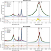 |
Fig. 1. Representative regions of optical nuclear spectrum (solid black lines) for MR 2251−178 (upper panels) and PG 1126−041 (lower panels), along with their respective best-fit models (solid red lines). The left-hand panels focus on the Hβ and [O III] lines, while the right-hand panels are centred on the Hα and [N II] lines. The models are given by the sum of the [Fe II] and Balmer emission lines from the nuclear region (solid purple and green lines, respectively), diffuse gas emission from individual atomic species (solid blue lines), and a third-order polynomial (dashed yellow lines). Emission from diffuse gas is modelled with three Gaussian components. Residuals (data minus model) are shown below each panel; red solid (black dashed) lines are used for models with (without) the BLR correction term (see text). The red vertical band in the bottom-right panels marks a region contaminated by a sky-subtraction residual and is not fitted by our model. |
3.2. Removing the contribution from the BLR
We then proceeded to remove the contamination of the BLR emission from the entire dataset. As the BLR was unresolved, we expected its emission to be spatially distributed like the MUSE PSF. The latter, given the AO-nature of our data, should be roughly made by a combination of an AO-corrected narrow core surrounded by a broad (seeing-limited) halo. The presence of this halo is particularly relevant, as bright sources – such as the BLR – can contaminate spaxels located far beyond the nominal spatial resolution. The exact shape of the PSF strongly depends on the observing conditions and is difficult to determine a priori, especially for AO observations.
To address this problem, we used pPXF software (Cappellari 2017) to model the whole datacube under the assumption that the contribution of the BLR emission to each spectrum is only a re-scaled version of that determined within the nuclear region. In practice, for each system, we produced a BLR template made by the sum of the best-fit [Fe II] lines, Balmer lines, and the polynomial found in Sect. 3.1. We then used pPXF to fit each spectrum in the datacube with a combination of our BLR template, which can only be re-scaled in amplitude, and multiple Gaussian components for the spatially resolved diffuse emission. With respect to the previous step, we allowed for a larger freedom in the modelling of the diffuse gas by assuming that the flux ratios of the different Gaussian components can vary freely amongst the different atomic species, so that different lines can have different total profiles. We still constrain the central velocities and velocity widths of all components to be the same in all the species considered, under the assumption of unique, underlying large-scale kinematics. Finally, the BLR component of the fit is subtracted to the original datacube, producing a “cleaned” cube containing only narrow lines from the various atomic species.
A couple of factors, however, complicate this procedure. A first concern is that the described approach leads to a poor fit to the spaxels around the centre, where the broad Hα and Hβ components appear to give different contributions to the spectrum with respect to what we inferred from the nuclear region. This issue is a consequence of the variation of the PSF with wavelength due to the AO-assisted nature of our data, with the Strehl ratio being higher in the red (Hα) than in the blue (Hβ). To account for this, we break the assumption of rigid re-normalisation of the full BLR model, which is instead split into two sub-regions (above and below the 5700 Å rest-frame) that can scale separately in the fit. Figure 2 shows a representative spectrum of MR 2251−178 to demonstrate that the approach described leads to a much better fit to the data in the regions around the Hβ line. Details on the MUSE PSF in the two spectral regions are provided in Appendix A.
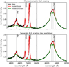 |
Fig. 2. Representative spectrum taken at 0.34″ from centre of MR 2251−178 (black lines in all panels), and best-fit models (red lines) derived by re-normalising the BLR contribution either as a whole (top panels), or for the red and blue regimes separately (bottom panels), as discussed in the text. The green lines show the contribution of the BLR emission to the full spectrum. The separate normalisation leads to a much better fit to the Hβ line (left panels). |
A second concern is the number of narrow components required to reproduce the data. This can vary across the field due to either an intrinsic variation in the complexity of the line profile, or to variations in the S/N. In order to decide the optimal number of components that are used in each spaxel, we adopted the following statistical approach. We first fit the whole datacube multiple times, each time using a fixed number of narrow components ranging from one to three. We found this range to be optimal given that even the most complex profile in our data can be accurately described by three components, while a single component is sufficient to model the fainter lines in the external part of the field of view, where the S/N is small, and the dynamics of the system are simpler. Then, for each spaxel we compared the distribution of the residual in a wavelength range encompassing the bright [O III] line using a Kolgomorov-Smirnov (KS) test. In practice, we ask whether the residuals of a model with n + 1 components differ statistically from those of a model with n components, starting from n = 1. If they do, we set n = n + 1 and re-do the test, otherwise we set to n the optimal number of components for that particular spaxel. This method does not rely on any particular likelihood estimator, and accounts only for the relative improvements that an additional fitted component would bring to the model. We can change our acceptance tolerance by varying the p-value threshold3 of the KS test. We experimented with different values and visually verified their effect on the final model, finding that 0.6 < p < 0.9 is the optimal range to describe our data. The fiducial p-values adopted are 0.75 for MR 2251−178 and 0.8 for PG 1126−041. Maps showing the number of components are presented in the section below.
3.3. Modelling the diffuse emission
In this step, we focused on the continuum and BLR-subtracted cubes to extract the properties of the emission lines from the diffuse ionised gas. While the latter were already modelled by pPXF in the procedure above, re-fitting these lines on the cleaned dataset brings two advantages. The first is that we have fewer free parameters, as we do not need to model the complex BLR emission. The second advantage consists of a larger freedom in selecting the desired functional forms to fit the data, bypassing the limitations of pPXF of using solely Gauss-Hermite functions. In practice, however, we found that a multi-Gaussian representation of the line profiles is perfectly satisfactory for the two datasets in question. In order to increase the S/N in the external regions of the datacube, we employed a Voronoi tessellation of our data using the method of Cappellari & Copin (2003). This consists of generating an adaptive spatial binning, with grid elements that can vary in size and shape, ensuring a minimum S/N across the whole dataset. We required each Voronoi bin to have a minimum S/N of 15 in the [O III] line4. The multi-Gaussian fit follows the same statistical methodology described in Sect. 3.2. In this step, we explicitly modelled the following emission lines: Hβ, [O III]λ4959, [O III]λ5007, [N II]λ6548, Hα, [N II]λ6583, [S II]λ6716, and [S II]λ6731. We treated the [O III] and [N II] lines as doublets, fixing both the [O III] λ5007/λ4959 line ratio and the [N II] λ6583/λ6548 line ratio to the theoretical value of 3. Fainter lines, such as [He I], [O I]λ6300 and [O I]λ6364, are detected (especially around the nuclear region) but not modelled.
The line shapes can be complex as they result from the mixture along the gas line of sight that follows the galaxy’s global kinematics with material showing strong “peculiar” motions (such as in an outflow). As the main target of our study is the outflowing gas, which is commonly traced by the broader component of the lines, we need to develop an automated method to separate it from the remaining “non-peculiar” kinematic component. For this purpose, we post-processed our best-fit model of the diffuse gas as follows.
For any given line profile, we first determined its peak velocity vpeak as the velocity corresponding to the line peak. We then flagged all Gaussian components that had at least a fraction, fHV, of their flux at relative velocities |v − vpeak| above a given threshold, vHV, as “high-velocity” (HV). If more than one component satisfies the condition above, these are merged together in a single HV component, and we label the remaining portion of the line profile as “low-velocity” (LV). This classification based on vpeak is well suited for our QSOs where emission lines from different species peak at similar velocities, and the HV components are always sub-dominant, but it may not be optimal in cases where vpeak varies significantly from one line to another or when the flux is dominated by the HV components. We note that, with the classification adopted, even lines described by a single component can be classified as HV if their velocity width is sufficiently large. After experimenting with different values, by visual inspection of the profiles we found that fHV = 0.4 and vHV = 300 km s−1 give the optimal separation between the HV and LV components. These values correspond to the requirement that about half of the flux in each HV component lies at velocities ≳3−4σ from the line peak, with σ being the typical velocity dispersion of the LV component (∼80−100 km s−1).
Figure 3 synthesises our modelling procedure for the diffuse gas. The number of components used in each Voronoi bin varies across the field (left-hand panes) and typically peaks in the central regions where the S/N is higher, decreasing at larger radii. Furthermore, MR 2251−178 shows a clear dichotomy where fewer components are required to reproduce the emission in the east-west direction (where the dense shells of the nebula lie) while more components are needed in the direction perpendicular to it. We discuss this further in Sect. 4.1. Individual line profiles are shown in the right-hand panels of Fig. 3. These are well fit by our model, and, in particular, the HV component accurately traces the extended blue wings of the emission lines. In the section below, we use these HV components to infer the properties of the outflowing gas.
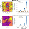 |
Fig. 3. Multi-component fit for diffuse gas emission lines of MR 2251−178 (top panels) and PG 1126−041 (bottom panels). Left-hand panels: iso-intensity contours for the integrated [O III] line (black lines); the background colours show the number of components used in each Voronoi bin. The [O III] maps are derived by integrating the (unbinned) BLR-subtracted cubes in the λλ4930−5030 Å rest-frame range and are spatially smoothed to a FWHM resolution of 0.25″. Contours are spaced by a factor of 2, the outermost being at 3× the rms noise. The crosses in cyan mark the bins at which the spectra shown in the right panels are extracted. Right-hand panels: representative spectra in a range encompassing the Hβ and [O III] lines for the BLR-subtracted cubes (black lines), our best-fit models (blue lines), and their HV sub-components alone (orange lines). |
4. Results
4.1. Distribution and kinematics of ionised gas
Figure 4 offers an overview of the distribution and the kinematics of the ionised gas in MR 2251−178 and PG 1126−041, as derived from our modelling of the [O III] and Hα lines. The moment-0 (intensity), moment-1 (velocity field), and moment-2 (dispersion field) maps for the LV and HV components of these lines are shown separately in order to better trace their distinct spatial and velocity distributions. The moment-1 and -2 maps are clipped to a peak S/N5 of 3. This significantly improves the quality of such maps, especially close to the borders, where contamination from HV components with a low S/N are important. Moment-2 maps have not been deconvolved for instrumental broadening, which gives minimum observable velocity dispersions σMUSE of about 50 km s−1 around the Hα line and 65 km s−1 around the [O III] doublet.
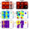 |
Fig. 4. Distribution and kinematics of diffuse ionised gas in MR 2251−178 (left-hand panels) and PG 1126−041 (right-hand panels). For each system, the set of six panels on top (middle, bottom) show the moment-0 (moment-1, moment-2) map for the [O III] (first row) and the Hα (second row) emission lines from diffuse gas. The different columns show the maps derived for the whole line, or for the LV and the HV components separately. Moment-1 and moment-2 maps are clipped at a peak S/N of 3. Moment-1 maps are relative to the systemic velocity of the QSOs, given by their estimated redshift. |
We focus first on the LV component in MR 2251−178, which dominates the diffuse gas emission beyond ∼0.5″ from the centre and traces the extended nebula around the galaxy very well. The nebula seems to be composed by a series of thin shells of ionised gas, which wrap around the system and extend in the east-west direction up to the edge of our field of view. Each shell shows several sub-structures that are particularly evident in the Hα intensity map, possibly because of the better spatial resolution achieved by the AO system at these wavelengths. The velocity field of the nebula is peculiar: while a clear velocity gradient is visible, its direction does not match the orientation of the shells perfectly. This mismatch suggests that the nebula cannot be described simply by a series of layers in spherical expansion from a central point, but that more complex kinematics are at work here. Furthermore, the moment-2 maps reveal that the material in the shell is described by an exceptionally low velocity dispersion (∼80 km s−1), of the order of the MUSE spectral resolution, which is at odds with expectations from a more turbulent AGN-driven wind origin. We discuss the origin of this nebula further in Sect. 5.1.
The LV component in PG 1126−041 is somewhat less spectacular. In this galaxy, the emission from diffuse gas is more centrally concentrated, and even for the brightest lines the S/N drops dramatically (and the Voronoi grid becomes very coarse) beyond the central ∼1″. Still, a large-scale velocity gradient seems to be visible, especially in the Hα line, which shows a velocity difference of about 350 km s−1 across its length. The LV Hα morphology and the orientation of its velocity gradient match those of the broad-band optical image of PG 1126−041 from the DSS6. We therefore interpret this velocity gradient as that of a regularly rotating disc, whose kinematics appear to be relatively undisturbed by the presence of an active galactic nucleus.
While the LV components preferentially trace the large-scale kinematics, the HV components are more informative of the nuclear activity. As expected, in both systems the HV component appears to be preferentially concentrated towards the galactic centre, featuring a negative (i.e. blue shifted) bulk velocity ranging from a few tens to a few hundreds of km s−1, and a velocity dispersion of 400−800 km s−1. These are all clear signs of the presence of AGN-driven outflows from the central regions of MR 2251−178 and PG 1126−041. We note that in both QSOs the HV component appears to be more spatially extended in [O III] than in Hα. This is likely caused by the different brightnesses of the two lines, with the HV-component of the latter falling below our S/N threshold beyond the central ∼1″. In MR 2251−178, the outflow appears to be extended in the north-south direction. The inferior S/N achieved in PG 1126−041 prevents us from studying the detailed spatial distribution of the outflow; yet, its size appears to be at least of ∼1″, thus much larger than the MUSE angular resolution (Fig. A.1). The energetics of these kpc-scale outflows and their connection to the sub-pc-scale X-ray wind are discussed in Sect. 4.3.
We focused here on the two brightest lines in our dataset, the [O III] and the Hα. We verified that the distribution and kinematics of the other atomic species that we modelled (Hβ, [N II], [S II]) were consistent with the pattern traced by these two lines, although their lower S/N strongly limits the study of the HV component.
4.2. Outflow electron densities
Converting the luminosity of the HV components into an outflow mass requires measurements of the wind electron density, ne. In general, ne can be estimated from the [S II]λ6716/[S II]λ6731 ratio (e.g. Osterbrock & Ferland 2006), which is measured in the regions of the outflow using the HV-components of the [S II] lines alone. Unfortunately, in both galaxies the [S II] doublet sits on top of the extended (red) wing of the BLR Hα line, and by visually inspecting our nuclear fits (Sect. 3.1) we find that the detailed shape of this wing is not accurately captured by our broken power-law BLR model. This biases our estimate of the [S II] fluxes, for which we need a different approach. We therefore made a new, ad-hoc model for a small spectral region surrounding the [S II] doublet (λλ6680−6780 rest-frame), consisting of a fifth-order polynomial for the BLR Hα wing, and two Gaussian components for each of the two [S II] lines, representing the low- and high-velocity parts of the doublet. Ideally, we should apply this model to the spectrum integrated within an aperture that fully encloses the outflow material. This can be done in PG 1126−041, where we extracted and modelled a series of spectra using various apertures within all the possible Rout (see Sect. 4.3), finding in all cases values for ne within ∼1000−2000 cm−3. Contrastingly, MR 2251−178 presents a strong velocity gradient in the region of its outflow (see moment-1 maps in Fig. 4), which would artificially broaden the [S II] lines when integrated over a large area. Thus, in this galaxy we used a much smaller aperture (0.05″), which we centred at different locations within the outflow region, finding values for ne within ∼500−1000 cm−3. The intervals of ne derived here are used in the next section to compute the masses of the outflowing ionised gas.
To illustrate the described approach, in Fig. 5 we show representative fits to the [S II] doublets. Clearly, both the Hα wings and the [S II] lines are very well reproduced, and the LV and HV-components are sufficiently separated. There are cases, however, where the component separation is more ambiguous, but we stress that our results would not vary significantly if we used the entire lines, rather than the HV components alone, to derive ne. We also note that the relation between the [S II] ratio and ne of Osterbrock & Ferland (2006), which we adopted in our calculations, is perfectly compatible with the recent re-calibration by Kewley et al. (2019) for the range of line ratios that we find.
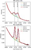 |
Fig. 5. [S II] emission lines and related models for MR 2251−178 (top panel) and PG 1126−041 (bottom panel). The black lines show the spectrum extracted within an aperture of 0.05″ (for MR 2251−178) and 0.5″ (for PG 1126−041) from the systems’ nuclei. The red lines show our best-fit models, with separate contributions from the wings of the BLR Hα (green lines), and the HV- and LV-components of the [S II] doublets (orange and blue lines, respectively). |
Given the emission lines available in our data, here we estimated the electron density using the “classical” method based on [S II] ratios. We note that the use of different density tracers (such as the auroral or transauroral lines, e.g. Holt et al. 2011) or of methods based on the ionisation parameter (e.g. Baron & Netzer 2019) tend to output densities higher by about one order of magnitude (Davies et al. 2020), and consequently lead to lower ionised gas masses (but see also Mingozzi et al. 2019, whose results suggests that these higher densities might be related to specific brighter and denser clumps that do not dominate the bulk of the outflow mass).
4.3. Outflow energetics
We now determine the physical properties of the kpc-scale outflow in MR 2251−178 and PG 1126−041. In what follows, we assume that the outflow material in the QSOs is traced by the HV components discussed in Sect. 4.1, and that it can be described as a collection of ionised gas clouds all having the same electron density ne7.
As before, we focused on the two brightest lines ([O III] and Hα) for which the HV components are more clearly visible, which we used as independent estimators for the outflow properties. Following Cresci et al. (2017), the mass of the outflowing ionised gas can be computed from the luminosity of the HV-Hα line  as
as
The same quantity can be derived from the HV-[O III] line, following (Cano-Díaz et al. 2012 see their Appendix B):
![$$ \begin{aligned} M_{\rm out}^\mathrm{[OIII]} = 5.33\times 10^4 \left(\frac{L_{\rm HV}^\mathrm{[OIII]}}{10^{40}\,\mathrm{erg\,s^{-1}}} \right) \left(\frac{100\,\mathrm{cm^{-3}}}{n_{\rm e}}\right) \frac{1}{10^\mathrm{[O/H]}}\,M_\odot , \end{aligned} $$](/articles/aa/full_html/2020/12/aa38889-20/aa38889-20-eq3.gif)
where 10[O/H] is the oxygen abundance in solar units.
The mass outflow rate, Ṁout, at a given radius Rout is derived using the simplified assumptions of spherical (or multi-conical) geometry and a constant outflow speed vout. Following Lutz et al. (2020), we have

where ℋ is a multiplicative factor that depends on the adopted outflow history. We assumed a temporally constant Ṁout during the flow time Rout/vout, which leads to a radially decreasing density for the outflowing gas (ρ ∝ R−2, i.e. an “isothermal” case) and gives ℋ = 1. This choice agrees with the “time-averaged thin-shell” approach (Rupke et al. 2005), and it has been extensively used in the literature to describe the energetics of the ionised and neutral phases of outflows (e.g. Arav et al. 2013; Heckman et al. 2015; González-Alfonso et al. 2017; Veilleux et al. 2017). We note that some other works preferred to adopt ℋ = 3 (e.g. Maiolino et al. 2012; Cicone et al. 2014; Feruglio et al. 2017), corresponding to a constant volume density for the outflowing gas as resulting from a decaying outflow history where Ṁout = 0 at the time. This is, however, at odds with the presence of UFOs in our sources.
The kinetic energy Ekin and luminosity Lkin (sometimes called “kinetic rate” and indicated as Ėkin) are given by
and, finally, the momentum rate ṗout is computed as
Equations (1)–(6) make use of different ingredients (vout, Rout, ne, luminosity and metallicity), most of which can be determined using our model for the HV components. In particular, we made use of “outflow velocity maps”, derived as follows for the two lines in question. For a given Voronoi bin k, we define the outflow velocity vout(k) as

where v5 and v95 are, respectively, the fifth and ninety-fifth velocity percentiles of the modelled HV profile in that bin, and vsys is the bulk (or systemic) velocity of the galaxy, given by its newly determined redshift. This definition is based on two assumptions. The first reflects our ignorance on the true morphology of the outflow and on its orientation with respect to the observer: as projection effects are unknown, we make the ansatz that what best represents the intrinsic outflow speed is the velocity tail of the profile, that is, the v5 or v95 in Eq. (7). These values are certainly better suited to represent vout than the mean (or median) velocity of the line, which is strongly affected by projection effects and by dust absorption (e.g. Cresci et al. 2015). The second assumption is that the outflow material comes from the nuclear region, and thus speeds must be computed with respect to the systemic velocity of the galaxy (the vsys in Eq. (7)) rather than to any other (local) reference frame. This is justified by the fact that the HV component indeed appears to be confined within the central region, as shown in Fig. 4.
Figure 6 shows maps for the two velocity terms that appear in Eq. (7) for the [O III] and Hα lines in MR 2251−178 and PG 1126−041. As before, only HV components with peak S/N above 3 are considered. As expected for an outflow traced by optical emission lines, |v5 − vsys|> |v95 − vsys| in virtually all spaxels, thus vout is, in practice, given by the first term alone. Both systems show maximum vout slightly above 1000 km s−1. Interestingly, in MR 2251−178 vout is larger at the centre and decreases at larger radii, which can be interpreted as due to projection effects in a spherically expanding wind. In PG 1126−041, instead, the kinematic pattern is less clear. In general, the outflows are not perfectly circular, and it is not straightforward to identify a characteristic outflow radius. However, under the assumption of constant Ṁout and vout, Eq. (3) is expected to hold at any Rout.
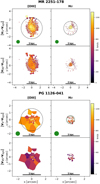 |
Fig. 6. Top panels: [O III] and Hα velocity maps showing fifth (first row) and ninety-fifth (second row) velocity percentiles of the HV components in MR 2251−178. The dashed circles show the maximum Rout adopted for the calculation of the momentum boost. The green filled circles indicate the size of the PSF halo, which is markedly smaller than the spatial extent of the data. Bottom panels: same as for PG 1126−041. The green dashed circle in the Hα panel shows the outflow radius corrected for the effect of the PSF. |
The empty circles drawn in Fig. 6 indicate the maximum possible outflow radius, Rmax, which we take as equal to the maximum spatial extent of the HV component in the lines analysed. Outflows in our QSOs are much more extended than the seeing-limited halos of the MUSE PSFs, which are shown as filled green circles with a radius of 2Rhalo (see Appendix A for the core/halo decomposition of the PSFs) in Fig. 6. This indicates that the outflows are spatially resolved. A correction such as  yields
  in all cases, with the largest difference occurring for the Hα outflow of PG 1126−041 (black vs. green dashed circles in Fig. 6).
To calculate the quantities in Eqs. (1)–(6), along with their associated uncertainty, we adopted a Monte Carlo approach where we randomly extracted N = 104 possible Rout between 0.5 × PSFFWHM, a proxy for the minimum resolved spatial scale (taken from Table A.1), and Rmax. The luminosity associated with a particular extraction was computed from the flux of the HV component within that aperture. Similarly, for vout we took a random velocity extracted within Rout from the maps shown in Fig. 4. For ne, we assumed a uniform distribution within the ranges determined in Sect. 4.2: 500−1000 cm−3 for MR 2251−178 and 1000−2000 cm−2 for PG 1126−041. For simplicity, we assumed the metallicity to be about solar, and we randomly sampled it in the −0.3 < [O/H] < 0.3 range. The Hα/Hβ flux ratios that we derive from integrated spectra of the HV components are consistent with negligible dust extinction, thus no corrections for the estimated luminosities are required.
With all the elements at our disposal, we then computed Eqs. (1)−(6) N times, take the medians of the resulting distributions as representative values for our measurements, and used the eighty-fourth and sixteenth percentiles for their upper and lower uncertainties. Table 2 summarises the outflow properties in MR 2251−178 and PG 1126−041, including our estimates for the kinetic efficiency Lkin/LBOL, and for the so-called “momentum boost”, that is the ratio between the momentum flux of the outflowing gas ṗout and the momentum flux initially provided by radiation pressure from the AGN (LBOL/c, where LBOL is taken from Table 1). Despite the limitations associated with these measurements, both the Hα and the [O III] lines give compatible values for the properties of the outflow in MR 2251−178 and PG 1126−041. In all cases, mass outflow rates are modest (0.6−4.3 M⊙ yr−1) and the kinetic efficiency is small (1−4 × 10⁻⁴). These values are in good agreement with the Ṁout − LBOL and Lkin − LBOL scaling relations reported by Fiore et al. (2017), which corroborates the validity of our method and indicates that MR 2251−178 and PG 1126−041 are similar to the bulk of the galaxy population featuring AGN-driven ionised winds.
Physical properties of the ionised outflow in MR 2251−178 and PG 1126−041 as derived from our analysis of the Hα and [O III] lines.
We discuss the implication of these findings on the physical mechanisms associated with the AGN wind further in Sect. 5.2. We stress that our analysis only accounts for the ionised component of the outflow, and it is indeed possible that the presence of a neutral (atomic and/or molecular) component may significantly increase the overall outflow mass and energy budget (e.g. Cicone et al. 2014; Fluetsch et al. 2019).
5. Discussion
5.1. The origin of the nebula around MR 2251−178
As we know from several previous studies (e.g. Bergeron et al. 1983; Macchetto et al. 1990; Shopbell et al. 1999), MR 2251−178 is surrounded by a a huge emission-line nebula, with a total size of ∼200 kpc and ionised gas mass of ∼6 × 10¹⁰ M⊙. Early kinematic estimates based on the Hα and [O III] lines indicate that the extended regions of the nebula counter-rotate with respect to the regions immediately surrounding the QSO (Norgaard-Nielsen et al. 1986; Shopbell et al. 1999), suggesting the presence of (at least) two distinct origins for the ionised gas around MR 2251−178. Different origins have been proposed for the extended nebula, including tidal debris from an interaction with a companion, debris from a major merging event, outflow from the QSO, cooling flow, or photo-ionisation of a large H I envelope. The latter option seems to be in better agreement with the regular large-scale kinematics suggested by the data. Unfortunately, interferometric H I data are not available for this source, and only a tentative Na I absorption feature is visible in our MUSE data, which is too faint to be modelled.
As our MUSE data only cover the innermost ∼12 × 12 kpc2 region, they cannot provide information on how the central regions are related to the outer parts. However, it is possible to confirm the counter-rotating nature of the inner nebula: we find red-shifted (blue-shifted) motion towards the east (west), in contrast with the large-scale kinematics found by Shopbell et al. (1999). Both the [S II] and the [N II] BPT diagrams, shown in Fig. 7, indicate that the AGN is by far the primary excitation driver for the nebula, although star formation may be relevant in the very centre and a few composite regions are present.
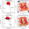 |
Fig. 7. Left panels: spatially resolved [S II]- and [N II]- BPT diagrams for MR 2251−178. Each dot corresponds to a single Voronoi bin. Red (blue) dots represent regions whose excitation is dominated by star formation (AGN), green dots are used for composite (in the [N II]-BPT) or LI(N)ER (in the [S II]-BPT) excitation regimes. Solid and dashed black lines show the separation between the different regimes, from Kewley et al. (2001, 2006) and Kauffmann et al. (2003). Only lines with S/N > 2 are used. Right panels: [S II]- and [N II]- BPT maps, colour-coded according to the dominant excitation regime. Darker colours indicate higher [S II] (top panel) or [N II] (bottom panel) intensities. Iso-intensity contours show the integrated [O III] line, smoothed to a FHWM resolution of 0.25″. The ionisation of the nebula is vastly dominated by the AGN. |
As discussed in Sect. 4.1, in spite of the fact that the ionised gas is structured in a series of shells, the low-velocity dispersion and the orientation of the velocity gradient in the LV component (see Fig. 4) do not favour gas outflowing from a past nuclear activity as an origin. Also, while the velocity gradient may recall that of a regularly rotating disc, the fact that velocities in the red-shifted region drop down to zero beyond a few kpc from the centre indicates that the inner nebula is not made by cold gas in circular orbits within the gravitational potential of the host. Instead, the complex morphology and kinematics of this nebula closely resemble those of the extended emission line regions (EELRs) around fading AGN studied by Keel et al. (2015), who concluded that photo-ionisation of tidal debris from minor mergers or flybys are the most likely origins for these structures.
Clearly, a detailed study of the metallicity of the ionised nebula is key to understand its origin. We attempted a first-order metallicity calculation using the procedure of Storchi-Bergmann et al. (1998), which made use of the [N II]/Hα and the [O III]/Hβ ratios alone and was specifically designed for the diffuse gas in active galaxies. Unfortunately, this resulted in a positive [O/H] gradient ranging from solar-like values at the centre of the nebula to ∼10 times solar at R ≃ 5 kpc, which we find unrealistic. We believe it is more likely that the gradients in line ratios are due to radial variations in the ionisation field rather than in the metal content. Interestingly, though, some numerical models of major mergers predict positive metallicity gradients for the merger remnant, as high-Z gas is moved inside-out by the enhanced AGN feedback activity (e.g. Cox et al. 2006). As MUSE wide field mode observations of this system are ongoing, we leave a more detailed study of the small- and large-scale metallicity structure of the nebula – along with its extended kinematics – to a future work.
5.2. Physical mechanisms for the wind propagation
Relating the momentum boost of these kpc-scale outflows to that derived for the sub-pc-scale high-speed (∼0.1c) wind traced by X-ray offers fundamental clues on the physical mechanism associated with the wind propagation. Following the theoretical model of King (2010), the X-ray wind is pushed by radiation pressure from the AGN and shock-heats the surrounding gas, inflating a hot bubble. Inverse-Compton is the primary cooling process at work, and the bubble evolution depends on the cooling timescale. For short cooling timescales, most of the bubble energy is radiated away, and the expanding (cold) shell communicates with the ambient medium only via its ram pressure, transferring its momentum flux to it (“momentum-driven” regime). Long timescales imply that the bubble keeps expanding while conserving its energy (“energy-driven” regime), efficiently sweeping up a considerable portion of the ISM and driving outflows of several thousands of M⊙ yr−1. This simple model may not capture additional effects due to the non-spherical geometry (Zubovas & Nayakshin 2014) or to the multi-phase nature of the wind (Faucher-Giguère & Quataert 2012), but has the considerable advantage of predicting an MBH − σ relation in broad agreement with the observations.
In Sect. 4.3, We already determined the momentum boosts for the galaxy-scale ionised outflows in MR 2251−178 and PG 1126−041. We now use X-ray measurements from the literature to determine the sub-pc-scale energetics in a similar manner. Following Nardini & Zubovas (2018), we assumed that the UFO was launched from the escape radius  , that is, the radius at which the observed outflow speed, vUFO, corresponds to the escape velocity from the black hole, and we write the mass outflow rate as

where Ω is the solid angle subtended by the wind, NH, UFO is the gas column density, and vUFO is the outflow speed. We took MBH, vUFO, and NH, UFO from Table 1 and assumed fiducial values of Ω/4π between 0.1 and 0.2, roughly corresponding to the detection rate of UFOs per source per observation in local AGN samples (e.g. Tombesi et al. 2010b). The UFO momentum rates, ṗUFO, were determined using a formula analogous to Eq. (6): we find  for PG 1126−041 and ≳0.19/(LBOL/c) (lower limit) for MR 2251−178.
Figure 8 shows the momentum boost as a function of the outflow speed for MR 2251−178 and PG 1126−041. Prediction for momentum conserving (energy conserving) winds are shown with dashed horizontal (dotted diagonal) lines originating from the X-ray data points. Error bars on the UFO momentum rates are large, especially in the case of MR 2251, where only a rough lower limit can be established. While these uncertainties are difficult to overcome, our measurements indicate that the momentum rate of the kpc-scale outflow is roughly compatible with that of the sub-pc-scale wind, favouring a “simple” momentum-driven scenario for these two galaxies. We note that, given the measured outflow velocities, an energy-driven scenario would be favoured only if the momentum fluxes were underestimated by about two orders of magnitude. Unless the AGN-driven outflow in MR 2251−178 and PG 1126−041 is completely dominated by a massive component of molecular gas, we find it unlikely that a perfectly energy-driven mechanism is at work here.
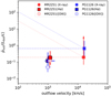 |
Fig. 8. Momentum boost for MR 2251−178 (red markers) and PG 1126−041 (blue markers) as a function of the outflow velocity. Crosses show the high-speed, sub-pc-scale wind observed in X-ray by Reeves et al. (2013) and Giustini et al. (2011) (see text). Filled and empty squares are used for the kpc-scale ionised outflow from the Hα and [O III] lines, respectively, as derived in this work. Dashed horizontal (dotted diagonal) lines show predictions for a momentum-driven (energy-driven) wind. |
However, the hypothesis of massive molecular outflows associated with these systems is not unrealistic. Various studies (e.g. Carniani et al. 2015; Fiore et al. 2017; Bischetti et al. 2019; Fluetsch et al. 2019) have compared molecular and ionised outflow rates in different AGN-hosting galaxies as a function of their LBOL. Given the typical LBOL of our galaxies (some 1045 erg s−1), outflow rates for a hypothetical molecular component may indeed exceed those measured for the ionised gas by a factor of ∼100. Unfortunately, the correlation between the different outflow phases is very uncertain, and only with dedicated molecular gas observations (e.g. with ALMA) can a more complete picture of the outflow properties in these systems be achieved.
5.3. Comparison with other QSOs
While the galaxy-scale (ionised) outflows in MR 2251−178 and PG 1126−041 appear to be propelled by momentum-driven winds, one may wonder whether the same occurs in other QSOs. In order to answer this question, we gathered high-quality measurements from the literature for another eight well-studied QSOs, including a lensed system at z ≃ 3.9 (APM 08279+5255), hosting both UFOs at sub-pc scales and galaxy-scale molecular/atomic outflows. For each of these sources, we re-computed the UFO mass outflow rate (and the wind energetics, subsequently) using Eq. (8), starting from known estimates for MBH, NH, UFO, and vUFO. All estimates for molecular outflows were re-scaled to the same luminosity-to-mass conversion factor, αCO = 0.8 (K km s−1 pc2)−1 M⊙, which is typical of QSOs and starburst and sub-millimetre galaxies (Downes & Solomon 1998; Carilli & Walter 2013; Bolatto et al. 2013). This allowed us to build a small, yet reliable high-quality sample for which the outflow properties were determined homogeneously. References for each system are given in Appendix B, and the detailed properties of pc- and galaxy-scale winds resulting from this analysis are listed in Table B.1. We present our main results below.
Figure 9 shows the ratio between the momentum rate of the galaxy-scale outflow (ṗout) and that of the pc-scale wind (ṗUFO) for all galaxies in our sample, and compares it to predictions for momentum-driven or energy-driven regimes (horizontal dashed line and orange rectangles, respectively). We reiterate that the ṗout values used for MR 2251−178 and PG 1126−041 refer to the ionised gas, and not to molecular/neutral outflow as in the other sources considered. Remarkably, with the exception of IRAS 17020+45448 all measurements for ṗout/ṗUFO seem to be compatible with one regime or the other, with no system being markedly located at an intermediate position. This demonstrates that the two theoretical regimes proposed, in spite of their simplicity, capture the physics of the AGN wind propagation very well.
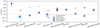 |
Fig. 9. Ratio between galaxy-scale and sub-pc-scale outflow momentum rates for different QSOs hosting UFOs. Measurements for individual galaxies are shown as squares (ionised outflows), circles (molecular outflows), and diamonds (atomic outflows) with error-bars. Systems are ordered by increasing LBOL. The horizontal dashed line shows the prediction for momentum-driven winds (ṗout/ṗUFO = 1), individual predictions for energy-driven winds are shown as orange rectangles. Our Hα and [O III] measurements for MR 2251−178 and PG 1126−041 are shown separately using filled and empty symbols, respectively. |
However, the interpretation of Fig. 9 is not straightforward, and two possible scenarios can be discussed. One possibility is that, at any given time, galaxy-scale winds are either in a momentum-driven or in an energy-driven regime, transiting from one regime to the other when certain physical conditions are met. Within the framework described by King & Pounds (2015), this transition may occur when central black holes have grown sufficiently to comply with the MBH − σ relation. When this happens, feedback transits from a little efficient (momentum-driven) phase, where the black hole still accretes material at a fast pace, to a highly efficient (energy-driven) regime, which causes the ejection of most of the ISM out of the galaxy, eventually quenching the black hole growth and star formation processes altogether. In this framework, the lack of intermediate regimes shown by Fig. 9 would indicate that the transition occurs over short timescales. Clearly, independent measurements for MBH and σ would be needed to test this hypothesis.
The scenario proposed, however, is not supported by most recent theoretical models of AGN feedback (e.g. Richings & Faucher-Giguère 2018; Costa et al. 2020), which predict energy-driven galaxy-scale outflows in virtually all cases. In this context, observed sub-energy-driven regimes would be attributed to an inefficient coupling between the UFO and the ISM, causing only part of the kinetic energy of the former to be transferred to the latter. As a possible counter-argument to this interpretation, we note the bimodality shown by the QSOs in Fig. 9 implies a coupling “efficiency factor” that is either ∼1 or very close to whatever value is required by the momentum-driven regime, which is somewhat difficult to justify. However, we stress that the observed bi-modality does not arise in similar studies on different QSO samples (e.g. Smith et al. 2019). A homogeneous, multi-phase study of a larger sample of QSOs hosting both sub-pc and galaxy-scale winds and featuring a wide range of LBOL is required to confirm the trend shown by Fig. 9.
5.4. Timescales
An important caveat associated with momentum boost arguments is that they implicitly assume that the QSO radiation force (LBOL/c) powering the pc-scale UFO is the same as that powering the galaxy-scale wind. However, flow timescales τflow ≡ Rout/vout for galaxy-scale outflows are of the order of the Myr, while LBOL can substantially vary on much shorter timescales. Therefore, comparing the energetics of the two components is done under the assumption that the LBOL measured at the current epoch, which powers the UFO, does not differ dramatically from the LBOL averaged over the entire duration of the flow. In this context, the exceptionally high ṗout of IRAS 17020+4544 can be interpreted as due to a much higher AGN luminosity at previous epochs, when the molecular outflow was launched. In fact, this is the only QSO in our sample for which τflow (∼2 Myr) is significantly lower than the time that the UFO would take to inject a total amount of kinetic energy equivalent to that of the large-scale wind (τkin ≡ Ekin/Lkin, UFO ∼ 60 Myr). This implies that the UFO and the molecular outflow that we observe in this system are not causally connected. Yet, the fact that all the other sources in Fig. 9 are compatible with the predicted regimes suggests that the underlying assumption of approximately constant LBOL over the flow time is physically motivated, at least for the targets presented here. Analogous considerations apply to the case where the UFO duty cycle is much shorter than the flow time.
6. Conclusions
Galaxy-wide winds produced by AGN are routinely observed around galaxies at all redshifts at which AGN are observed. They are thought to have a fundamental impact on galaxy evolution, in particular by quenching star formation in high-mass systems. Despite substantial observational efforts, the physical mechanism by which the wind propagates from the (sub-pc-scale) nuclear region to the (kpc-scale) interstellar medium, eventually leading to galaxy-scale outflows, is still elusive. Progress in this direction can only be achieved by studying the properties of the wind on different physical scales (e.g. Tombesi et al. 2015, 2017; Feruglio et al. 2015; Veilleux et al. 2017; Smith et al. 2019; Bischetti et al. 2019; Mizumoto et al. 2019; Gaspari et al. 2020).
To pursue this methodology, in this work we used MUSE NF-mode data to study the properties of the ionised gas around two systems, MR 2251−178 (z = 0.064) and PG 1126−041 (z = 0.060), which host massive, sub-pc-scale, ultra-fast (∼0.1c) outflows visible via blue-shifted Fe K absorption line in their nuclear X-ray spectrum (Gofford et al. 2011; Giustini et al. 2011). Our MUSE data cover a region of about 12 × 12 kpc2 around the nucleus, and have sensitivity, spatial and spectral resolutions that are optimal to study the kinematics of the ionised gas from the Hα and [O III] emission lines. We employed a method based on a multi-component analysis of the line profiles, which allowed us to disentangle the large-scale emission of the diffuse gas from the nuclear (unresolved) emission of the BLR, as the latter contaminates the whole field of view due to the extended wings of the MUSE AO-assisted PSF. Emission from diffuse gas is further decomposed into a HV component, which traces the large-scale, more turbulent outflowing material, and an LV component, which exhibits more regular and quiet kinematics.
Our results can be summarised as follows.
-
In both systems, the HV component is spatially concentrated within a few kpc of the centre and features a HV dispersion (up to ∼800 km s−1) and a mean blue-shifted speed of several tens of km s−1 in MR 2251−178, or a few hundred km s−1 in PG 1126−041. Undoubtedly, this component traces a nuclear outflow driven by the AGN.
-
The LV component in MR 2251−178 is structured in a series of concentric shells distributed in the east-west direction, tracing the inner regions of the giant (200 kpc-wide) ionised nebula that surrounds this galaxy. Its kinematics show a clean velocity gradient, which is misaligned with respect to the orientation of the shells, and a low-velocity (∼80 km s−1) dispersion. We speculate that tidal debris from recent minor mergers or flybys can explain the observed properties of this structure.
-
An LV component in PG 1126−041 is likely associated with the regularly rotating disc of the galaxy, which does not seem to be perturbed by the nuclear activity.
-
Outflows are characterised by small mass rates (0.6−4.3 M⊙ yr−1) and poor kinetic efficiencies (1−4 × 10⁻⁴).
-
The momentum rates associated with the large-scale Hα and [O III] outflows are compatible with those inferred from the sub-pc-scale measurements in the X-rays, which is in agreement with a momentum-driven wind propagation. Pure energy-driven winds were excluded unless our outflow rates were underestimated by about two orders of magnitude, which may occur in the presence of a massive molecular wind.
-
We compared the outflow energetics of MR 2251−178 and PG 1126−041 with those of a small sample of well-studied QSOs from the literature, each hosting both sub-pc-scale UFOs and molecular and/or atomic winds on galaxy scales. We find that, in all systems but one, winds are either in a momentum-driven or in an energy-driven regime. Uncertainties associated with the variability of the UFOs and the UFO-to-ISM coupling efficiency prevent us from establishing whether or not the observed bi-modality is intrinsic to the physics of AGN-driven winds.
A caveat associated with this study is the lack of information on atomic or molecular gas, which prevents us from determining in full the outflow energetics in the two QSOs in question. Follow-up observations (e.g. with ALMA) are essential to obtaining a more complete picture of the outflow properties in these systems and to provide useful constraints to AGN-driven wind theories.
Retrievable from the NASA/IPAC Extragalactic Database: https://ned.ipac.caltech.edu/
A variable cloud density implies a non-unitary multiplicative factor  in Eqs. (1) and (2). A constant ne yields 𝒞 = 1 (Cano-Díaz et al. 2012).
For which ṗout is very uncertain; see discussion in Longinotti et al. (2018, Sect. 3.1).
Acknowledgments
AM and GC acknowledge the support by INAF/Frontiera through the “Progetti Premiali” funding scheme of the Italian Ministry of Education, University, and Research. EN acknowledges financial support from the agreement ASI-INAF n.2017-14-H.0. EP acknwoledges financial support from ASI/INAF contract 2017-14-H.0 and from PRIN MIUR project “Black Hole winds and the Baryon Life Cycle of Galaxies: the stone-guest at the galaxy evolution supper”.
References
- Arav, N., Borguet, B., Chamberlain, C., Edmonds, D., & Danforth, C. 2013, MNRAS, 436, 3286 [NASA ADS] [CrossRef] [Google Scholar]
- Baron, D., & Netzer, H. 2019, MNRAS, 486, 4290 [NASA ADS] [CrossRef] [Google Scholar]
- Baron, D., Netzer, H., Davies, R. I., & Xavier Prochaska, J. 2020, MNRAS, 494, 5396 [Google Scholar]
- Bergeron, J., Boksenberg, A., Dennefeld, M., & Tarenghi, M. 1983, MNRAS, 202, 125 [NASA ADS] [CrossRef] [Google Scholar]
- Bischetti, M., Piconcelli, E., Vietri, G., et al. 2017, A&A, 598, A122 [NASA ADS] [CrossRef] [EDP Sciences] [Google Scholar]
- Bischetti, M., Piconcelli, E., Feruglio, C., et al. 2019, A&A, 628, A118 [Google Scholar]
- Bolatto, A. D., Wolfire, M., & Leroy, A. K. 2013, ARA&A, 51, 207 [Google Scholar]
- Booth, C. M., & Schaye, J. 2009, MNRAS, 398, 53 [Google Scholar]
- Braito, V., Reeves, J. N., Matzeu, G. A., et al. 2018, MNRAS, 479, 3592 [Google Scholar]
- Brusa, M., Bongiorno, A., Cresci, G., et al. 2015, MNRAS, 446, 2394 [NASA ADS] [CrossRef] [Google Scholar]
- Cano-Díaz, M., Maiolino, R., Marconi, A., et al. 2012, A&A, 537, L8 [NASA ADS] [CrossRef] [EDP Sciences] [Google Scholar]
- Cappellari, M. 2017, MNRAS, 466, 798 [NASA ADS] [CrossRef] [Google Scholar]
- Cappellari, M., & Copin, Y. 2003, MNRAS, 342, 345 [NASA ADS] [CrossRef] [Google Scholar]
- Carilli, C. L., & Walter, F. 2013, ARA&A, 51, 105 [NASA ADS] [CrossRef] [EDP Sciences] [Google Scholar]
- Carniani, S., Marconi, A., Maiolino, R., et al. 2015, A&A, 580, A102 [NASA ADS] [CrossRef] [EDP Sciences] [Google Scholar]
- Chartas, G., Saez, C., Brandt, W. N., Giustini, M., & Garmire, G. P. 2009, ApJ, 706, 644 [Google Scholar]
- Cicone, C., Feruglio, C., Maiolino, R., et al. 2012, A&A, 543, A99 [NASA ADS] [CrossRef] [EDP Sciences] [Google Scholar]
- Cicone, C., Maiolino, R., Sturm, E., et al. 2014, A&A, 562, A21 [NASA ADS] [CrossRef] [EDP Sciences] [Google Scholar]
- Cicone, C., Brusa, M., Ramos Almeida, C., et al. 2018, Nat. Astron., 2, 176 [Google Scholar]
- Ciotti, L., & Ostriker, J. P. 1997, ApJ, 487, L105 [NASA ADS] [CrossRef] [Google Scholar]
- Ciotti, L., Pellegrini, S., Negri, A., & Ostriker, J. P. 2017, ApJ, 835, 15 [NASA ADS] [CrossRef] [Google Scholar]
- Cooke, B. A., Lawrence, A., & Perola, G. C. 1978, MNRAS, 182, 661 [CrossRef] [Google Scholar]
- Costa, T., Pakmor, R., & Springel, V. 2020, MNRAS, 497, 5229 [CrossRef] [Google Scholar]
- Cox, T. J., Di Matteo, T., Hernquist, L., et al. 2006, ApJ, 643, 692 [NASA ADS] [CrossRef] [Google Scholar]
- Cresci, G., Mainieri, V., Brusa, M., et al. 2015, ApJ, 799, 82 [Google Scholar]
- Cresci, G., Vanzi, L., Telles, E., et al. 2017, A&A, 604, A101 [NASA ADS] [CrossRef] [EDP Sciences] [Google Scholar]
- Dasyra, K. M., Tacconi, L. J., Davies, R. I., et al. 2006, ApJ, 638, 745 [NASA ADS] [CrossRef] [Google Scholar]
- Davies, R., Baron, D., Shimizu, T., et al. 2020, MNRAS, 498, 4150 [Google Scholar]
- di Serego Alighieri, S., Perryman, M. A. C., & Macchetto, F. 1984, ApJ, 285, 567 [NASA ADS] [CrossRef] [Google Scholar]
- Downes, D., & Solomon, P. M. 1998, ApJ, 507, 615 [NASA ADS] [CrossRef] [Google Scholar]
- Fabian, A. C. 2012, ARA&A, 50, 455 [Google Scholar]
- Faucher-Giguère, C.-A., & Quataert, E. 2012, MNRAS, 425, 605 [NASA ADS] [CrossRef] [Google Scholar]
- Feruglio, C., Maiolino, R., Piconcelli, E., et al. 2010, A&A, 518, L155 [NASA ADS] [CrossRef] [EDP Sciences] [Google Scholar]
- Feruglio, C., Fiore, F., Carniani, S., et al. 2015, A&A, 583, A99 [NASA ADS] [CrossRef] [EDP Sciences] [Google Scholar]
- Feruglio, C., Ferrara, A., Bischetti, M., et al. 2017, A&A, 608, A30 [NASA ADS] [CrossRef] [EDP Sciences] [Google Scholar]
- Fiore, F., Feruglio, C., Shankar, F., et al. 2017, A&A, 601, A143 [NASA ADS] [CrossRef] [EDP Sciences] [Google Scholar]
- Fluetsch, A., Maiolino, R., Carniani, S., et al. 2019, MNRAS, 483, 4586 [NASA ADS] [Google Scholar]
- Freudling, W., Romaniello, M., Bramich, D. M., et al. 2013, A&A, 559, A96 [NASA ADS] [CrossRef] [EDP Sciences] [Google Scholar]
- Ganguly, R., Charlton, J. C., & Eracleous, M. 2001, ApJ, 556, L7 [CrossRef] [Google Scholar]
- Gaspari, M., Temi, P., & Brighenti, F. 2017, MNRAS, 466, 677 [NASA ADS] [CrossRef] [Google Scholar]
- Gaspari, M., Tombesi, F., & Cappi, M. 2020, Nat. Astron., 4, 10 [CrossRef] [Google Scholar]
- Gibson, R. R., Marshall, H. L., Canizares, C. R., & Lee, J. C. 2005, ApJ, 627, 83 [CrossRef] [Google Scholar]
- Giustini, M., Cappi, M., Chartas, G., et al. 2011, A&A, 536, A49 [NASA ADS] [CrossRef] [EDP Sciences] [Google Scholar]
- Gofford, J., Reeves, J. N., Turner, T. J., et al. 2011, MNRAS, 414, 3307 [CrossRef] [Google Scholar]
- Gofford, J., Reeves, J. N., Tombesi, F., et al. 2013, MNRAS, 430, 60 [Google Scholar]
- Gofford, J., Reeves, J. N., McLaughlin, D. E., et al. 2015, MNRAS, 451, 4169 [Google Scholar]
- González-Alfonso, E., Fischer, J., Spoon, H. W. W., et al. 2017, ApJ, 836, 11 [NASA ADS] [CrossRef] [Google Scholar]
- Hagino, K., Done, C., Odaka, H., Watanabe, S., & Takahashi, T. 2017, MNRAS, 468, 1442 [NASA ADS] [CrossRef] [Google Scholar]
- Halpern, J. P. 1984, ApJ, 281, 90 [NASA ADS] [CrossRef] [Google Scholar]
- Hamann, F., Chartas, G., Reeves, J., & Nardini, E. 2018, MNRAS, 476, 943 [NASA ADS] [CrossRef] [Google Scholar]
- Hao, C. N., Xia, X. Y., Mao, S., Wu, H., & Deng, Z. G. 2005, ApJ, 625, 78 [NASA ADS] [CrossRef] [Google Scholar]
- Harrison, C. M. 2017, Nat. Astron., 1, 0165 [NASA ADS] [CrossRef] [Google Scholar]
- Harrison, C. M., Alexander, D. M., Swinbank, A. M., et al. 2012, MNRAS, 426, 1073 [NASA ADS] [CrossRef] [Google Scholar]
- Heckman, T. M., Alexandroff, R. M., Borthakur, S., Overzier, R., & Leitherer, C. 2015, ApJ, 809, 147 [NASA ADS] [CrossRef] [Google Scholar]
- Holt, J., Tadhunter, C. N., Morganti, R., & Emonts, B. H. C. 2011, MNRAS, 410, 1527 [NASA ADS] [Google Scholar]
- Hopkins, P. F., & Elvis, M. 2010, MNRAS, 401, 7 [NASA ADS] [CrossRef] [Google Scholar]
- Huang, Y.-K., Hu, C., Zhao, Y.-L., et al. 2019, ApJ, 876, 102 [CrossRef] [Google Scholar]
- Kauffmann, G., Heckman, T. M., Tremonti, C., et al. 2003, MNRAS, 346, 1055 [Google Scholar]
- Keel, W. C., Maksym, W. P., Bennert, V. N., et al. 2015, AJ, 149, 155 [NASA ADS] [CrossRef] [Google Scholar]
- Kewley, L. J., Dopita, M. A., Sutherland, R. S., Heisler, C. A., & Trevena, J. 2001, ApJ, 556, 121 [Google Scholar]
- Kewley, L. J., Groves, B., Kauffmann, G., & Heckman, T. 2006, MNRAS, 372, 961 [NASA ADS] [CrossRef] [Google Scholar]
- Kewley, L. J., Nicholls, D. C., Sutherland, R., et al. 2019, ApJ, 880, 16 [NASA ADS] [CrossRef] [Google Scholar]
- King, A. 2003, ApJ, 596, L27 [NASA ADS] [CrossRef] [Google Scholar]
- King, A. R. 2010, MNRAS, 402, 1516 [NASA ADS] [CrossRef] [Google Scholar]
- King, A., & Pounds, K. 2015, ARA&A, 53, 115 [Google Scholar]
- Komossa, S., & Meerschweinchen, J. 2000, A&A, 354, 411 [NASA ADS] [Google Scholar]
- Kormendy, J., & Ho, L. C. 2013, ARA&A, 51, 511 [Google Scholar]
- Kovačević, J., Popović, L. Č., & Dimitrijević, M. S. 2010, ApJS, 189, 15 [NASA ADS] [CrossRef] [Google Scholar]
- Longinotti, A. L., Krongold, Y., Guainazzi, M., et al. 2015, ApJ, 813, L39 [NASA ADS] [CrossRef] [EDP Sciences] [Google Scholar]
- Longinotti, A. L., Vega, O., Krongold, Y., et al. 2018, ApJ, 867, L11 [NASA ADS] [CrossRef] [Google Scholar]
- Lusso, E., Comastri, A., Vignali, C., et al. 2010, A&A, 512, A34 [NASA ADS] [CrossRef] [EDP Sciences] [Google Scholar]
- Lutz, D., Sturm, E., Janssen, A., et al. 2020, A&A, 633, A134 [NASA ADS] [CrossRef] [EDP Sciences] [Google Scholar]
- Macchetto, F., Colina, L., Golombek, D., Perryman, M. A. C., & di Serego Alighieri, S. 1990, ApJ, 356, 389 [NASA ADS] [CrossRef] [Google Scholar]
- Maiolino, R., Gallerani, S., Neri, R., et al. 2012, MNRAS, 425, L66 [NASA ADS] [CrossRef] [Google Scholar]
- Mingozzi, M., Cresci, G., Venturi, G., et al. 2019, A&A, 622, A146 [NASA ADS] [CrossRef] [EDP Sciences] [Google Scholar]
- Mizumoto, M., Izumi, T., & Kohno, K. 2019, ApJ, 871, 156 [CrossRef] [Google Scholar]
- Morganti, R., Tadhunter, C. N., & Oosterloo, T. A. 2005, A&A, 444, L9 [NASA ADS] [CrossRef] [EDP Sciences] [Google Scholar]
- Nardini, E., & Zubovas, K. 2018, MNRAS, 478, 2274 [Google Scholar]
- Nardini, E., Reeves, J. N., Porquet, D., et al. 2014, MNRAS, 440, 1200 [CrossRef] [Google Scholar]
- Nardini, E., Reeves, J. N., Gofford, J., et al. 2015, Science, 347, 860 [Google Scholar]
- Norgaard-Nielsen, H. U., Hansen, L., Jorgensen, H. E., & Christensen, P. R. 1986, A&A, 169, 49 [NASA ADS] [Google Scholar]
- Osterbrock, D. E., & Ferland, G. J. 2006, Astrophysics of Gaseous Nebulae and Active Galactic Nuclei (Sausalito: University Science Books) [Google Scholar]
- Pan, H. C., Stewart, G. C., & Pounds, K. A. 1990, MNRAS, 242, 177 [NASA ADS] [CrossRef] [Google Scholar]
- Phillips, M. M. 1980, ApJ, 236, L45 [NASA ADS] [CrossRef] [Google Scholar]
- Pontzen, A., Tremmel, M., Roth, N., et al. 2017, MNRAS, 465, 547 [Google Scholar]
- Pounds, K. A., Reeves, J. N., King, A. R., et al. 2003, MNRAS, 345, 705 [NASA ADS] [CrossRef] [Google Scholar]
- Reeves, J. N., & Braito, V. 2019, ApJ, 884, 80 [Google Scholar]
- Reeves, J. N., O’Brien, P. T., Braito, V., et al. 2009, ApJ, 701, 493 [NASA ADS] [CrossRef] [Google Scholar]
- Reeves, J. N., Porquet, D., Braito, V., et al. 2013, ApJ, 776, 99 [NASA ADS] [CrossRef] [Google Scholar]
- Richards, G. T., Lacy, M., Storrie-Lombardi, L. J., et al. 2006, ApJS, 166, 470 [NASA ADS] [CrossRef] [Google Scholar]
- Richings, A. J., & Faucher-Giguère, C.-A. 2018, MNRAS, 474, 3673 [Google Scholar]
- Ricker, G. R., Clarke, G. W., Doxsey, R. E., et al. 1978, Nature, 271, 35 [NASA ADS] [CrossRef] [Google Scholar]
- Rothberg, B., Fischer, J., Rodrigues, M., & Sanders, D. B. 2013, ApJ, 767, 72 [NASA ADS] [CrossRef] [Google Scholar]
- Rupke, D. S., Veilleux, S., & Sanders, D. B. 2005, ApJS, 160, 115 [NASA ADS] [CrossRef] [Google Scholar]
- Rupke, D. S. N., Gültekin, K., & Veilleux, S. 2017, ApJ, 850, 40 [Google Scholar]
- Saturni, F. G., Bischetti, M., Piconcelli, E., et al. 2018, A&A, 617, A118 [NASA ADS] [CrossRef] [EDP Sciences] [Google Scholar]
- Shopbell, P. L., Veilleux, S., & Bland-Hawthorn, J. 1999, ApJ, 524, L83 [NASA ADS] [CrossRef] [Google Scholar]
- Silk, J. 2013, ApJ, 772, 112 [NASA ADS] [CrossRef] [Google Scholar]
- Silk, J., & Rees, M. J. 1998, A&A, 331, L1 [NASA ADS] [Google Scholar]
- Sirressi, M., Cicone, C., Severgnini, P., et al. 2019, MNRAS, 489, 1927 [CrossRef] [Google Scholar]
- Smith, R. N., Tombesi, F., Veilleux, S., Lohfink, A. M., & Luminari, A. 2019, ApJ, 887, 69 [NASA ADS] [CrossRef] [Google Scholar]
- Storchi-Bergmann, T., Schmitt, H. R., Calzetti, D., & Kinney, A. L. 1998, AJ, 115, 909 [NASA ADS] [CrossRef] [Google Scholar]
- Tombesi, F., Cappi, M., Reeves, J. N., et al. 2010a, A&A, 521, A57 [NASA ADS] [CrossRef] [EDP Sciences] [Google Scholar]
- Tombesi, F., Sambruna, R. M., Reeves, J. N., et al. 2010b, ApJ, 719, 700 [NASA ADS] [CrossRef] [Google Scholar]
- Tombesi, F., Cappi, M., Reeves, J. N., et al. 2011, ApJ, 742, 44 [Google Scholar]
- Tombesi, F., Cappi, M., Reeves, J. N., & Braito, V. 2012, MNRAS, 422, L1 [NASA ADS] [CrossRef] [Google Scholar]
- Tombesi, F., Cappi, M., Reeves, J. N., et al. 2013, MNRAS, 430, 1102 [Google Scholar]
- Tombesi, F., Meléndez, M., Veilleux, S., et al. 2015, Nature, 519, 436 [Google Scholar]
- Tombesi, F., Veilleux, S., Meléndez, M., et al. 2017, ApJ, 850, 151 [NASA ADS] [CrossRef] [Google Scholar]
- Veilleux, S., Meléndez, M., Sturm, E., et al. 2013, ApJ, 776, 27 [NASA ADS] [CrossRef] [Google Scholar]
- Veilleux, S., Bolatto, A., Tombesi, F., et al. 2017, ApJ, 843, 18 [Google Scholar]
- Vestergaard, M., & Peterson, B. M. 2006, ApJ, 641, 689 [NASA ADS] [CrossRef] [Google Scholar]
- Wang, T., & Lu, Y. 2001, A&A, 377, 52 [NASA ADS] [CrossRef] [EDP Sciences] [Google Scholar]
- Wang, T. G., Brinkmann, W., Wamsteker, W., Yuan, W., & Wang, J. X. 1999, MNRAS, 307, 821 [NASA ADS] [CrossRef] [Google Scholar]
- Weinberger, R., Springel, V., Hernquist, L., et al. 2017, MNRAS, 465, 3291 [NASA ADS] [CrossRef] [Google Scholar]
- Woo, J.-H., Bae, H.-J., Son, D., & Karouzos, M. 2016, ApJ, 817, 108 [NASA ADS] [CrossRef] [Google Scholar]
- Zubovas, K., & King, A. 2012, ApJ, 745, L34 [Google Scholar]
- Zubovas, K., & Nayakshin, S. 2014, MNRAS, 440, 2625 [NASA ADS] [CrossRef] [Google Scholar]
Appendix A: The AO-assisted PSF of MUSE NFM
In this appendix, we describe the MUSE NFM PSFs derived from our modelling of the BLRs in two different spectral regimes, as discussed in Sect. 3.2. The PSF maps, obtained by integrating the BLR models over the λλ4800−4900 Å (the “blue” regime) and λλ6500−6650 Å (the “red” regime) rest-frame ranges, are shown in Fig. A.1, together with their azimuthally-averaged profiles. The full width at half maximum (FWHM) of the PSF profile in MR 2251−178 (PG 1126−041) is 76 (46) mas for the red regime and 106 (68) mas for the blue regime. However, most of the light falls far beyond such distances: in MR 2251−178 (PG 1126−041), half of the total energy is enclosed within a diameter of 440 (270) mas in the red and 640 (440) mas in the blue. These estimates are reported in Table A.1 (along with the MUSE velocity resolution in the red and blue regimes) and clearly indicate that, as expected, the AO works better at longer wavelengths, leading to a more centrally concentrated PSF (i.e. a higher Strehl ratio). Also, the MUSE data for PG 1126−041 have better angular resolutions that those of MR 2251−178, which is in agreement with the superior seeing conditions during the observations (∼0.48″ vs. ∼0.84″). Overall, the fact that our BLR-traced PSFs agree with expectations from AO-assisted observational techniques is an excellent validation of our BLR modelling scheme, and, in general, a promising starting point for our analysis.
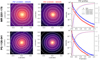 |
Fig. A.1. MUSE AO-assisted PSF for MR 2251−178 (top panels) and PG 1126−041 (bottom panels) as traced by intensity of BLR emission. Leftmost and central panels: separate PSF maps for the blue regime (λλ4800−4900 Å) and for the red regime (λλ6500−6650 Å). Each map is normalised to its peak value. Iso contours are the same for all maps and spaced by a factor of 2. Rightmost panels: azimuthally averaged PSF profiles (empty squares, one data point in every three is plotted for better clarity) and the enclosed energy fraction (thick dashed lines). The solid lines show our best-fit models, given by the sum of a Gaussian core (dotted lines) and a Moffat halo (thin dashed lines). |
We further decomposed the PSF profiles into the sum of a core and a halo component, which we modelled with a Gaussian and a Moffat profile, respectively. This model has four free parameters (one for the core, two for the halo, plus the normalisation), which we fitted to the data to determine their optimal
Main PSF properties and velocity resolution of our MUSE data for two different spectral ranges, λλ4800−4900 Å (“blue”) and λλ6500−6650 Å (“red”).
values. In all cases, we find a unique and well-defined minimum χ2 in the parameter space9. Our best-fit model gives a very good description of the PSF profiles, as shown in the rightmost panels of Fig. A.1.
We define core and halo “radii”, Rcore and Rhalo, as the standard deviations of the Gaussian and Moffat components. These values are used to compare the PSFs with the spatial extent of the outflows in Sect. 4.3 and are reported at the bottom of Table A.1, along with the fraction of the total light enclosed within the core, fcore.
Appendix B: Supplementary m aterial
Table B.1 lists the main parameters used in the calculation of the UFO and the galaxy-scale outflow energetics for the QSOs studied in Sect. 5.3. We provide the appropriate references for each system below.
Main physical properties for the QSOs studied in Sect. 5.3, and for their pc-scale and galaxy-scale winds.
IRAS 05189+2524. We estimated the black hole mass from the MBH − σ relation (Kormendy & Ho 2013) using the two values of σ determined by Dasyra et al. (2006, 137 km s−1) and Rothberg et al. (2013, 265 km s−1) as a range. Moreover, LBOL was taken from Veilleux et al. (2013), while the UFO velocity and column density were taken from Smith et al. (2019). The galaxy-scale outflow is seen via different tracers: CO (Lutz et al. 2020), OH (González-Alfonso et al. 2017), and Na (Rupke et al. 2017). The OH and Na phases dominate the energetics, and we sum them for the purpose of determining the global outflow properties.
In the I Zw 1 system, MBH was accurately measured by Huang et al. (2019) via a dedicated reverberation mapping campaign. We took LBOL from Veilleux et al. (2013) and the properties of the X-ray wind from Reeves & Braito (2019), who also determined a large value for the wind-covering factor (here we assume Ω/4π = 0.5). A CO wind is undetected in this QSO. Instead, there is evidence for a neutral outflow (Rupke et al. 2017), which we used in our calculations.
For PDS 456, we adopted the MBH determined by Nardini et al. (2015) using the λ5100 Å luminosity and the Hβ FWHM. We took the averaged LBOL from two different estimates: the first from the λ5100 Å luminosity with bolometric correction (Richards et al. 2006), and the second using the λ1350 Å luminosity from Hamann et al. (2018). The properties of the X-ray UFO come from Nardini et al. (2015), where they specifically determined a wind opening angle Ω/4π of 0.5. A galaxy-scale outflow was detected in CO by Bischetti et al. (2019) and consists of an extended component, in turn partitioned into four different blobs, and a compact component, which largely dominates the energetics of the system. For the purpose of measuring the outflow energetics, we considered both components together.
With Mrk 231, as for PDS 456, MBH was derived using the λ5100 Å luminosity and the Hβ FWHM (from Nardini & Zubovas 2018). We took LBOL from Veilleux et al. (2013), and the X-ray wind velocity and NH, UFO from Feruglio et al. (2015). The molecular (CO) outflow energetics come from Lutz et al. (2020), who used data originally from Cicone et al. (2012). A large-scale outflow is also observed in OH González-Alfonso et al. (2017), but with properties that are compatible with those of the wind detected in CO. Following Nardini & Zubovas (2018), we assumed the CO-based estimates as representative for the large-scale outflow.
For the system IRAS F11119+3257, MBH also comes from the λ5100 Å luminosity and the Hβ FWHM (from Nardini & Zubovas 2018), and LBOL from Veilleux et al. (2013). X-ray wind properties are from Tombesi et al. (2015). Molecular outflows are observed in both OH (Tombesi et al. 2015) and CO (Veilleux et al. 2017), but on different physical scales, with the former being confined within 1 kpc from the centre and the latter being visible at greater (∼15 kpc) distances. It is therefore likely that the two molecules trace distinct outflow episodes. For simplicity, we only show the CO energetics, but that determined for the OH is compatible within the quoted uncertainties.
Concerning IRAS 17020+4544, we inferred the black hole mass from the MBH − σ relation of Kormendy & Ho (2013) using the [O III] velocity dispersion (125 km s−1Wang & Lu 2001) as a proxy for the stellar σ. We bracketed the value of LBOL using two measurements: the first from the λ5100 Å (Hao et al. 2005) and the second (more conservative) from that assumed in Longinotti et al. (2015), from which we also took the X-ray wind properties. The properties of the CO molecular outflow are from Lutz et al. (2020). In Longinotti et al. (2018), the outflow properties of this QSO were found to be compatible with an energy-driven regime (although with large uncertainties). The differences here are due to the factor of ∼5 lower covering factor assumed for the UFO, and the factor of ∼20 lower gas column density, which arised as we interpreted the entry  in Table 2 of Longinotti et al. (2015) as a truncated Gaussian distribution, leading to a median log(NH, UFO/cm−2) ≃ 22.73.
For MCG-03-58-007, as before, MBH was inferred from the MBH − σ using the [O III] velocity dispersion (185 km s−1, Braito et al. 2018) as a proxy for σ. The LBOL is bracketed by the two values quoted in Braito et al. (2018), determined using either [O III] or IR luminosities. From the same work, we took the properties of the X-ray wind, for which we considered only the slowest of the two components observed, which is the only one persisting in different observations. The properties of the CO outflows were taken from Sirressi et al. (2019).
With APM 08279+5255, unlike the other systems considered, this is a lensed QSO at z ≃ 3.9. While lens models cannot very accurately constrain the value of the magnification μ, on which most quantities relevant to this analysis depend, indirect methods indicate μ = 4 as the best possible choice (Saturni et al. 2018). We considered this value for the magnification and took MBH and LBOL from Saturni et al. (2018). The X-ray wind properties come from Chartas et al. (2009), using only the slowest component (see their Table 3, model 8, absorber 1), which was also identified separately by Hagino et al. (2017). The properties of the CO molecular outflow are taken from Feruglio et al. (2017) using their model with μ = 4.
All Tables
Physical properties of the ionised outflow in MR 2251−178 and PG 1126−041 as derived from our analysis of the Hα and [O III] lines.
Main PSF properties and velocity resolution of our MUSE data for two different spectral ranges, λλ4800−4900 Å (“blue”) and λλ6500−6650 Å (“red”).
Main physical properties for the QSOs studied in Sect. 5.3, and for their pc-scale and galaxy-scale winds.
All Figures
|
Fig. 1. Representative regions of optical nuclear spectrum (solid black lines) for MR 2251−178 (upper panels) and PG 1126−041 (lower panels), along with their respective best-fit models (solid red lines). The left-hand panels focus on the Hβ and [O III] lines, while the right-hand panels are centred on the Hα and [N II] lines. The models are given by the sum of the [Fe II] and Balmer emission lines from the nuclear region (solid purple and green lines, respectively), diffuse gas emission from individual atomic species (solid blue lines), and a third-order polynomial (dashed yellow lines). Emission from diffuse gas is modelled with three Gaussian components. Residuals (data minus model) are shown below each panel; red solid (black dashed) lines are used for models with (without) the BLR correction term (see text). The red vertical band in the bottom-right panels marks a region contaminated by a sky-subtraction residual and is not fitted by our model. |
| In the text | |
|
Fig. 2. Representative spectrum taken at 0.34″ from centre of MR 2251−178 (black lines in all panels), and best-fit models (red lines) derived by re-normalising the BLR contribution either as a whole (top panels), or for the red and blue regimes separately (bottom panels), as discussed in the text. The green lines show the contribution of the BLR emission to the full spectrum. The separate normalisation leads to a much better fit to the Hβ line (left panels). |
| In the text | |
|
Fig. 3. Multi-component fit for diffuse gas emission lines of MR 2251−178 (top panels) and PG 1126−041 (bottom panels). Left-hand panels: iso-intensity contours for the integrated [O III] line (black lines); the background colours show the number of components used in each Voronoi bin. The [O III] maps are derived by integrating the (unbinned) BLR-subtracted cubes in the λλ4930−5030 Å rest-frame range and are spatially smoothed to a FWHM resolution of 0.25″. Contours are spaced by a factor of 2, the outermost being at 3× the rms noise. The crosses in cyan mark the bins at which the spectra shown in the right panels are extracted. Right-hand panels: representative spectra in a range encompassing the Hβ and [O III] lines for the BLR-subtracted cubes (black lines), our best-fit models (blue lines), and their HV sub-components alone (orange lines). |
| In the text | |
|
Fig. 4. Distribution and kinematics of diffuse ionised gas in MR 2251−178 (left-hand panels) and PG 1126−041 (right-hand panels). For each system, the set of six panels on top (middle, bottom) show the moment-0 (moment-1, moment-2) map for the [O III] (first row) and the Hα (second row) emission lines from diffuse gas. The different columns show the maps derived for the whole line, or for the LV and the HV components separately. Moment-1 and moment-2 maps are clipped at a peak S/N of 3. Moment-1 maps are relative to the systemic velocity of the QSOs, given by their estimated redshift. |
| In the text | |
|
Fig. 5. [S II] emission lines and related models for MR 2251−178 (top panel) and PG 1126−041 (bottom panel). The black lines show the spectrum extracted within an aperture of 0.05″ (for MR 2251−178) and 0.5″ (for PG 1126−041) from the systems’ nuclei. The red lines show our best-fit models, with separate contributions from the wings of the BLR Hα (green lines), and the HV- and LV-components of the [S II] doublets (orange and blue lines, respectively). |
| In the text | |
|
Fig. 6. Top panels: [O III] and Hα velocity maps showing fifth (first row) and ninety-fifth (second row) velocity percentiles of the HV components in MR 2251−178. The dashed circles show the maximum Rout adopted for the calculation of the momentum boost. The green filled circles indicate the size of the PSF halo, which is markedly smaller than the spatial extent of the data. Bottom panels: same as for PG 1126−041. The green dashed circle in the Hα panel shows the outflow radius corrected for the effect of the PSF. |
| In the text | |
|
Fig. 7. Left panels: spatially resolved [S II]- and [N II]- BPT diagrams for MR 2251−178. Each dot corresponds to a single Voronoi bin. Red (blue) dots represent regions whose excitation is dominated by star formation (AGN), green dots are used for composite (in the [N II]-BPT) or LI(N)ER (in the [S II]-BPT) excitation regimes. Solid and dashed black lines show the separation between the different regimes, from Kewley et al. (2001, 2006) and Kauffmann et al. (2003). Only lines with S/N > 2 are used. Right panels: [S II]- and [N II]- BPT maps, colour-coded according to the dominant excitation regime. Darker colours indicate higher [S II] (top panel) or [N II] (bottom panel) intensities. Iso-intensity contours show the integrated [O III] line, smoothed to a FHWM resolution of 0.25″. The ionisation of the nebula is vastly dominated by the AGN. |
| In the text | |
|
Fig. 8. Momentum boost for MR 2251−178 (red markers) and PG 1126−041 (blue markers) as a function of the outflow velocity. Crosses show the high-speed, sub-pc-scale wind observed in X-ray by Reeves et al. (2013) and Giustini et al. (2011) (see text). Filled and empty squares are used for the kpc-scale ionised outflow from the Hα and [O III] lines, respectively, as derived in this work. Dashed horizontal (dotted diagonal) lines show predictions for a momentum-driven (energy-driven) wind. |
| In the text | |
|
Fig. 9. Ratio between galaxy-scale and sub-pc-scale outflow momentum rates for different QSOs hosting UFOs. Measurements for individual galaxies are shown as squares (ionised outflows), circles (molecular outflows), and diamonds (atomic outflows) with error-bars. Systems are ordered by increasing LBOL. The horizontal dashed line shows the prediction for momentum-driven winds (ṗout/ṗUFO = 1), individual predictions for energy-driven winds are shown as orange rectangles. Our Hα and [O III] measurements for MR 2251−178 and PG 1126−041 are shown separately using filled and empty symbols, respectively. |
| In the text | |
|
Fig. A.1. MUSE AO-assisted PSF for MR 2251−178 (top panels) and PG 1126−041 (bottom panels) as traced by intensity of BLR emission. Leftmost and central panels: separate PSF maps for the blue regime (λλ4800−4900 Å) and for the red regime (λλ6500−6650 Å). Each map is normalised to its peak value. Iso contours are the same for all maps and spaced by a factor of 2. Rightmost panels: azimuthally averaged PSF profiles (empty squares, one data point in every three is plotted for better clarity) and the enclosed energy fraction (thick dashed lines). The solid lines show our best-fit models, given by the sum of a Gaussian core (dotted lines) and a Moffat halo (thin dashed lines). |
| In the text | |
Current usage metrics show cumulative count of Article Views (full-text article views including HTML views, PDF and ePub downloads, according to the available data) and Abstracts Views on Vision4Press platform.
Data correspond to usage on the plateform after 2015. The current usage metrics is available 48-96 hours after online publication and is updated daily on week days.
Initial download of the metrics may take a while.