| Issue |
A&A
Volume 644, December 2020
|
|
|---|---|---|
| Article Number | A128 | |
| Number of page(s) | 21 | |
| Section | Interstellar and circumstellar matter | |
| DOI | https://doi.org/10.1051/0004-6361/202037895 | |
| Published online | 10 December 2020 | |
VLA ammonia observations of L1287
Analysis of the Guitar core and two filaments
1
Departament de Física Quàntica i Astrofísica, Institut de Ciències del Cosmos, Universitat de Barcelona, (IEEC-UB) Martí i Franquès, 1,
08028
Barcelona,
Spain
e-mail: robert.estalella@ub.edu
2
Instituto de Astrofísica de Andalucía, CSIC,
Glorieta de la Astronomía, s/n,
18008
Granada,
Spain
3
Departament de Física i Enginyeria Nuclear, Universitat Politècnica de Catalunya, Av. Eduard Maristany 16,
08019
Barcelona,
Catalunya,
Spain
4
Institut de Ciències de l’Espai (ICE, CSIC),
Campus UAB, Carrer de Can Magrans, s/n,
08193,
Cerdanyola del Vallès,
Catalunya,
Spain
5
Institut d’Estudis Espacials de Catalunya (IEEC),
08034,
Barcelona,
Catalunya,
Spain
6
Instituto de Radioastronomía y Astrofísica, Universidad Nacional Autónoma de México,
PO Box 3-72,
58090,
Morelia,
Michoacán,
Mexico
Received:
6
March
2020
Accepted:
2
November
2020
Aims. In this paper, we study the dense gas of the molecular cloud LDN 1287 (L1287), which harbors a double FU Ori system, an energetic molecular outflow, and a still-forming cluster of deeply embedded low-mass young stellar objects that show a high level of fragmentation.
Methods. We present optical Hα and [SII], and VLA NH3 (1, 1) and (2, 2) observations with an angular resolution of ~3′′.5. The observed NH3 spectra have been analyzed with the Hyperfine Structure tool, fitting simultaneously three different velocity components.
Results. The NH3 emission from L1287 comes from four different structures: a core associated with RNO 1, a guitar-shaped core (the Guitar) and two interlaced filaments (the blue and red filaments) roughly centered toward the binary FU Ori system RNO 1B/1C and its associated cluster. Regarding the Guitar core, there are clear signatures of gas infall onto a central mass that has been estimated to be ~2.1M⊙. Regarding the two filaments, they have radii of ~0.03 pc, masses per unit length of ~50M⊙ pc−1, and are in near isothermal equilibrium. A central cavity is identified, probably related with the outflow and also revealed by the Hα and [SII] emission, with several young stellar objects near its inner walls. Both filaments show clear signs of perturbation by the high-velocity gas of the outflows driven by one or several young stellar objects of the cluster. The blue and red filaments are coherent in velocity and have nearly subsonic gas motions, except at the position of the embedded sources. Velocity gradients across the blue filament can be interpreted either as infalling material onto the filament or rotation. Velocity gradients along the filaments are interpreted as infall motions toward a gravitational well at the intersection of the two filaments.
Key words: ISM: general / ISM: individual objects: LDN 1287 / stars: formation
© ESO 2020
1 Introduction
Filaments are prevailing structures in star-forming regions, as revealed by the large-scale images obtained by the Herschel Space Observatory (e.g., André et al. 2010; Molinari et al. 2010; Arzoumanian et al. 2011; Stutz, & Kainulainen 2015; Schisano et al. 2020). Most of the known prestellar and protostellar dense cores lie along such filamentary structures (e.g., Polychroni et al. 2013; Könyves et al. 2015). Filaments and their intersections, called hubs, are thought to constitute the essential bricks building molecular clouds (e.g., Myers 2009). In this scenario, filaments collapsing toward the densest parts of molecular clouds lead to the formation of stellar clusters (e.g., Krumholz et al. 2018).
LDN 1287 (hereafter L1287) is the densest part of a large-scale filament (~ 100 pc) shown by dust emission at 160, 250, 350, and 500 μm observed by Herschel (Schisano et al. 2020; Juárez et al. 2019, see Fig. 1), and is located at a distance of  pc (Rygl et al. 2010). The dense gas in the region has been mapped in HCN, HCO+ (Yang et al. 1991), NH3 (Estalella et al. 1993; Sepúlveda 2001; Sepúlveda et al. 2011), CS (Yang et al. 1995; McMuldroch et al. 1995), and dust continuum emission (Sandell & Weintraub 2001). The mass in the central 0.5 pc of radius has been estimated from the C18 O emission to be ~ 120M⊙ (Umemoto et al. 1999).
L1287 contains an energetic bipolar molecular outflow with its axis in the northeast–southwest direction (Snell et al. 1990; Yang et al. 1991; Xu et al. 2006; Fehér et al. 2017; Juárez et al. 2019). A very cold and luminous IRAS point source, IRAS 00338+6312, with an estimated bolometric luminosity of 760 L⊙ (Connelley et al. 2007) is located toward the center of the outflow. A binary FU Ori system, RNO 1B/1C, whose components are separated by ~ 6″, is also found afew arcsec southwest of the nominal IRAS position (Staude & Neckel 1991; Kenyon et al. 1993). Given the large uncertainty in the IRAS position a debate was raised to clarify whether the IRAS source and the FU Ori system were the same objects, or if the IRAS source actually is an independent object (Weintraub & Kastner 1993), presumably younger and more embedded than the optically visible FU Ori system (classified as Class II objects; Quanz et al. 2007), which would be the driving source of the molecular outflow. This issue was clarified by the results of the radio continuum observations by Anglada et al. (1994) who detect a 3.6 cm counterpart, VLA 3, of the IRAS source. The accurate position of the radio source clearly indicates the presence of an embedded young stellar object independent of the FU Ori binary, a result further supported by the detection of H2 O maser emission associated with VLA 3 (Fiebig 1995, 1997) and the more recent detection of a mid-infrared (mid-IR) counterpart (Quanz et al. 2007), providing a refined IR position, which is fully in agreement with the centimeter position. The source VLA 3, as imaged by Anglada et al. (1994) shows the characteristics of a thermal radio jet, and is elongated along the outflow axis, making it the best candidate to power the molecular outflow. This association with the outflow has been confirmed by recent SMA CO (2–1) maps of the outflow by Juárez et al. (2019) that show that VLA 3 is the source closest to the origin of the bipolar outflow (see Sect. 4.1).
Several studies propose that L1287 harbors a cluster in the process of formation. In addition to the protostar associated with the IRAS–VLA source and the binary FU Ori system, there are three additional VLA sources (one of them, VLA 1, very close to the position of RNO 1C) that could associated with YSOs. More recently, Quanz et al. (2007) find four additional mid-IR sources tentatively classified as Class 0/I and Class II objects (one of them, the Class 0/I RNO 1G, very close to the position of VLA 2), which suggest that RNO 1B and 1C belong to a young small stellar cluster, making them the only well-studied and confirmed FU Ori stars that apparently belong to a cluster-like environment. Interestingly, both FU Ori stars, RNO 1B and 1C, have been detected in X-rays with Chandra (Skinner & Güdel 2020). Juárez et al. (2019), from 1.3 mm continuum SMA images, find a large number of dust peaks, some of them close to the positions of the YSOs identified at other wavelengths, inferring a very high fragmentation level in the L1287 core (see right panel of Fig. 1) compared to fragmentation in other samples of massive dense cores. Juárez et al. (2019) also propose, based on large-scale and small-scale kinematic motions of L1287, that converging flows toward the center of the filamentary structure are responsible for the formation of the cluster of YSOs, but other interpretations cannot be ruled out to explain the complex kinematics, such as outflow feedback and superposition of individual velocity components.
In this paper, we report optical Hα and [SII] observations, and VLA observations of the ammonia (1, 1) and (2, 2) inversion transitions with an angular resolution of ~ 3′′.5 to study the kinematics and physical properties of the dense gas at the center of L1287. The data presented here allowed us to disentangle at least three different velocity components that seem to be interacting with each other and feeding the central region of the long filament of L1287. In Sect. 2, we describe the observations and the spectral line analysis, in Sect. 3 we present the results, in Sect. 4 we discuss the results obtained for the Guitar core and the blue and red filaments, and in Sect. 5 we give our conclusions. Finally, in Appendix A we show additional observational data, in Appendix B we develop the self-gravitating isothermal cylindrical filament model used to fit the blue and red filament structure, and in Appendix C we summarize the expressions of the free-fall velocity and free-fall time for a cylindrical filament.
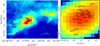 |
Fig. 1 Herschel large-scale map (left) of H2 column density (Juárez et al. 2019). The large-scale filament, roughly in the southeast–northwest direction, can be clearly seen. The large box shows the region mapped in NH3, encompassing the area of highest column density of the filament. The embedded sources detected in the IR, millimeter, and centimeter continuum are identified in the enlarged view (right) of the small box in the central area (except RNO 1, which lies outside the small box). The black dots (•) in the right panel correspond to millimeter dust-continuum emission (Juárez et al. 2019), and the plus signs (+) to mid-IR sources (Quanz et al. 2007) and centimeter continuum sources (Anglada et al. 1994). |
2 Observations and data analysis
2.1 VLA NH3 observations
Observations of the (J, K) = (1, 1) and (J, K) = (2, 2) inversion transitions of the ammonia molecule (at the rest frequencies 23.694495 and 23.722633 GHz, respectively) were carried out with the VLA of the NRAO1 in the D configuration in 1996, August 31 (Project code: AA198; P.I.: G. Anglada). The phase center of the interferometer was set at the position of the catalogue position of IRAS 00338+6312, α(J2000) = 00h36m47.s7, δ(J2000) = +63°29′02″.
The absolute flux calibrator was 3C48 (0134+329) for which a flux density of 1.1 Jy at the observed frequency of 23.7 GHz was adopted. The phase calibrator was 0224+671, with a bootstrapped flux density of 1.82 Jy, and 0316+413 was used as bandpass calibrator.
The NH3 (1, 1) and (2, 2) lines were observed simultaneously using the four-IF spectral mode of the VLA, which allows the observation of two polarizations for each line. A bandwidth of 3.125 MHz was used, with 63 channels of 48.828 kHz width (0.618 km s−1 at λ = 1.3 cm) centered on VLSR = −18.0 km s−1. Calibration and data reduction were performed using standard procedures of the Astronomical Imaging Processing System (AIPS) of the NRAO. Cleaned maps were obtained with the task IMAGR of AIPS. The resulting synthesized beam size, after natural weighting of the visibility data, was 3′′. 69 × 3′′.29 (PA =1. ° 6) and the achieved 1σ noise level per spectral channel was 3 mJy beam−1 (equivalent to 0.54 K of beam-averaged brightness temperature).
2.2 CAHA optical observations
The L1287 field was observed with the 2.2 m telescope of the Calar Alto Observatory (CAHA) in 2016, November, within a program to image the optical counterparts of IRAS-source YSOs candidates (Autumn 2016 #12; P.I.: A. Riera; López et al. 2020).
Deep CCD narrow-band images were obtained using the Calar Alto Faint Object Spectrograph (CAFOS) with the SITe chip, which gives an image scale of 0′′. 53 pixel−1 and a field of view of ~16′. Three narrow-band filters were used: an Hα filter (central wavelength λ = 6569 Å, bandpass Δλ = 50 Å), an [SII] filter (central wavelength λ = 6744 Å, bandpass Δλ = 97 Å) that included the emission from the [SII] λ = 6717, 6731Å lines, and an additional filter of central wavelength λ = 6607Å, bandpass Δλ = 43Å) to obtain the continuum adjacent to the Hα and [SII] emission lines.
We obtained images in Hα and [SII] of 1 h of total integration time by combining three frames of 1200 s exposure each, and an additional continuum image of 1200 s integration after combining two frames of 600 s exposure. All the images were processed with the standard tasks of the IRAF2 reduction package, which included bias subtraction and flatfielding corrections using sky flats. In order to correct for the misalignment among individual frames, the frames were recentered using the reference positions of field stars well distributed around the source.
Astrometric calibration of the images was performed in order to compare the optical emission with the positions of the radio continuum sources. The images were registered using the (α, δ) coordinates from the USNO Catalogue3 of ten field stars well distributed on the observed field. The rms of the transformation was 0′′. 2 in both coordinates.
2.3 NH3 hyperfine fitting analysis
The NH3 (1, 1) and (2, 2) lines were analyzed by means of the Hyperfine Structure (HfS) tool (Estalella 2017). This tool simultaneously fits the hyperfine quadrupole and magnetic structure of the NH3 (1, 1) and (2, 2) inversion transitions, with the assumptions that the beam filling factor, the excitation temperature, the hyperfine line width, and the central velocity are the same for all the hyperfine lines. In addition, the HfS tool uses the results of the fit to derive physical parameters including the excitation temperature, NH3 column density, rotational and kinetic temperature, with the assumption that the emitting region is homogeneous along the line of sight.
Despite the relatively low spectral resolution of the observations (0.618 km s−1), the spectra showed the presence of several velocity components in the emission, which were apparent in different positions of the region (see also the channel maps in Figs. A.1, A.2, and A.3). After careful inspection of the spectra, three different velocity components were identified, with non-overlapping velocity ranges, valid for all the region mapped. The range of velocities for each component were − 20.16 to − 18.31 km s−1 (component 1), − 18.31 to − 17.07 km s−1 (component 2), and − 17.07 to − 14.60 km s−1 (component 3). In Fig. 2, we show the (1, 1) and (2, 2) spectra at selected positions where only one of the components is present (top three rows) and either two or all three components are present (bottom three rows). The positions where the spectra were taken are given in the figure.
The HfS tool was used to fit simultaneously three velocity components of the (1, 1) and (2, 2) transitions, each one inside the velocity range given above. The fit was performed for the central 256 × 256 pixels of the map. For each pixel (pixel size 0′′.6), the (1, 1) and (2, 2) spectra were averaged within a boxcar of 3″ in diameter. We checked that no information was lost with the smoothing, and the fits were more reliable due to the enhanced signal-to-noise ratio. The fit was performed for pixels where the main beam brightness temperature of both lines was higher than 2.0 K (four times the typical rms noise level). Some examples of the fits for the different components are shown in Fig. 2. In total, the fit was performed for 3728 pixels, with component 1 fitted in 1318 pixels, component 2 in 2537 pixels, and component 3 in 1005 pixels. For each component fitted in each pixel, six line parameters were obtained from the fit: (1) hyperfine-line full width at half maximum (deconvolved from the channel width), ΔV, the same for the (1, 1) and (2, 2) transitions; (2) (1, 1) central velocity, VLSR1; (3) amplitude A4 times the (1, 1) main component optical depth, Aτ1m; (4) (1, 1) main component optical depth, τ1m; (5) (2, 2) central velocity, VLSR2; and (6) amplitude A times the (2, 2) main component optical depth, Aτ2m. In addition, physical parameters were obtained, for example Trot, Tk, and N(NH3) (see Estalella 2017, for a detailed description of the parameters), which were used in the analysis of the physical characteristics of the region. FITS images for the fitted parameters for each velocity component were produced by the HfS tool.
With the aim of characterizing the kinematics of the gas, an additional run of the HfS three-component fit was performed to fit only the (1, 1) spectra, irrespective of the intensity of the (2, 2) emission. For this run the fit was performed for 8420 pixels, with component 1 fitted in 2262 pixels, component 2 in 6633 pixels, and component 3 in 2858 pixels. For pixels fitted in both runs ((1, 1) and (2, 2) simultaneously, and (1, 1) only) the values of the(1, 1) line parameters fitted in the second run showed no significant differences from the values fitted in the first run.
The spectra with best signal-to-noise ratio have fit uncertainties in VLSR on the order of 0.02–0.11 km s−1, in ΔV on the order of 0.05–0.09 km s−1, and in Trot on the order of 1.4–3.8 K. The errors were greater for spectra whose signal-to-noise ratios were not as good, and the median values of the errors in VLSR, ΔV, and Trot are given in Table 1. The results were inspected for bad fits. As a general rule, fits with values of ΔV > 1.5 km s−1, or errors in ΔV > 1.0 km s−1, which in general corresponded to fits of a low-intensity, very wide component, were considered artifacts and were blanked out. After blanking, 3593 pixels remained with (1, 1) and (2, 2) fits, and 8371 pixels with fits of the (1, 1) line only.
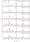 |
Fig. 2 Examples of NH3 (1, 1) (left) and (2, 2) (right) spectra in L1287: observed (black), fitted component 1 (green), component 2 (blue), component 3 (red). The dotted vertical lines show the range of velocities used for fitting the three velocity components. From top to bottom: position A, component 1 only; B, component 2 only; C, component 3 only; D, components 1 and 3; E, components 2 and 3; F, all three components present. The coordinates of the six positions are given in the right panels. |
3 Results
The morphology of the region is dominated by a large-scale filament, several parsec long, in a roughly southeast–northwest direction, clearly visible in the H2 column density (Fig. 1) and dust temperature maps obtained from Herschel data (Juárez et al. 2019). Our VLA ammonia observations show details of the dense gas distributed in extended filaments in a region of ~ 1′.5 in diameter encompassing both RNO 1, a background young star with 2MASS counterpart, at a distance of 1.24 ± 0.05 kpc (Gaia Collaboration 2018), and the RNO 1B/1C objects. The Hα and [SII] images show strong emission associated with the RNO 1 and RNO 1B/1C objects.
3.1 Hα and [SII] emission
The Hα and [SII] images obtained show a very similar morphology. The image of the [SII] emission, characteristic of shock-excited ionization, is presented in Fig. 3 in the top panel and that of Hα in the bottom panel. The strong emission in the upper left corner corresponds to RNO 1, and two field stars appear near the left and right borders of the image.
Regarding the emission at the center of the image, the strongest [SII] and Hα emission comes from a compact region (~10″ or ~9000 au), which encompasses the positions of the two stars of the FU Ori binary RNO 1B/1C, while the positions of IRAS–VLA 3, RNO 1F, RNO 1G–VLA 2, and VLA 4 fall in the periphery where the emission is weaker. The optical emission at the central region most probably traces the central cavity detected in the near-IR by Kenyon et al. (1993), where the extinction is lower.
There is faint [SII] and Hα emission elongated in the direction of the axis of the bipolar CO outflow that appears associated with its blue lobe, as mapped by Juárez et al. (2019) (see Fig. 3). There is no emission detected in association with the outflow red lobe, due probably to a higher extinction.
3.2 Ammonia emission: characterization of the different velocity components
In Appendix A, we show the channel maps of the observed NH3 (1, 1) main line (Fig. A.1) and inner satellites (Fig. A.2), and the NH3 (2, 2) line (Fig. A.3). The positions of the known YSOs thought to be associated with the region are indicated in these figures. The NH3 (1, 1) and (2, 2) spectra toward the positions of these YSOs are shown in Fig. A.4.
In Fig. 4, we show the integrated intensity map of the three velocity components of the NH3 emission identified in L1287 through the HfS analysis. In order of increasing velocity component 1 (hereafter Guitar core, see discussion below) is shown in gray scale and black contours, component 2 (corresponding to the RNO 1 core and the blue filament) in blue contours, and component 3 (hereafter red filament) in red contours.
In general, the three velocity components trace different parts of the high-density gas, with a few locations where there is superposition of more than one component (see Figs. 2 and 4). There are pixels in these regions for which the assignment of emission to the second or third velocity components could not be doneaccurately with the present spectral resolution. This occurs mainly in the southward extension of the eastern part of the blue filament, where there is emission of the southeast blob of the red filament, and in the westernmost part of the blue filament, where there is also some emission from the red filament (see Fig. 4).
In Table 1, we give the median values and 1σ equivalent dispersion for all the pixels with a fitted spectrum for RNO 1, the Guitar core, and the blue and red filaments, of the values of VLSR, ΔV, Trot, and N(NH3).
The NH3 (1, 1) integrated line-intensity maps corrected for opacity (AτmΔV) of the three components are shown in Fig. 5 in contours. The embedded YSOs are also indicated in this figure. As can be seen in the figure, the emission from the Guitar core (top panel) is compact (the body of the guitar), with a diameter of ~ 26″ (0.12 pc) plus an extension to the northwest (the neck of the guitar), with a length of ~ 36″ (0.16 pc). The emission of the blue and red filaments (middle and bottom panels) is instead elongated and twisted. The length of the blue filament is on the order of 120″ (0.52 pc), and that of the red filament of 90″ (0.40 pc). The width of both filaments is on the order of 20″ (0.10 pc). The length and width of the blue and red filaments in NH3 are much smaller than that of the dusty filamentary structure, as recently reported in the Herschel HiGAL catalogue (Schisano et al. 2020). The Herschel dust filament has a length of 6.1 pc and a width of 0.24 pc. These larger values are expected since the dust filament seen by Herschel extends well beyond the region mapped in NH3, which traces the densest part (close to the spine) of the filament. The main part of the blue filament (middle panel) is roughly in the east–west direction, and bends northward at the location of the embedded sources. A gap in the NH3 emission, at the position of the embedded YSOs, separates this main part from another clump of emission with no clear elongation to the west of the main part in the direction of the large-scale filament traced by Herschel (see Fig. 1). The red filament (bottom panel) has a general direction southeast to northwest, compatible with the filament oriented at PA = 34°4 reported in the Hi-GAL catalogue (Schisano et al. 2020).
Figure 5 also shows, in color scale, the beam-averaged NH3 column density, calculated assuming a beam filling factor f = 1. In this and the following figures, the portion of the figures that shows contours but no color scale are pixels that were fitted with only the NH3 (1, 1) line. The median value for all pixels fitted for each component, and the 1σ dispersion are given in Table 1. As can be seen, the median column density of the Guitar core is higher than that of the filaments. The masses of the Guitar and filaments were obtained from the integration of the column density maps after applying the primary beam correction (see Table 1). The values obtained assuming an ammonia abundance X(NH3) = 1 × 10⁻⁸ are 30 M⊙ (Guitar core), 104 M⊙ (blue filament), and 13 M⊙ (red filament).
The velocity component from − 18.31 to − 17.07 km s−1 also traces emission from a core encompassing the position of RNO 1, ~ 40″ (~ 0.17 pc) north of the main part of the blue filament (middle panel in Figs. 5, 6, and 7). The RNO 1 core presents narrow lines (ΔV ≃ 0.27 km s−1), with a central velocity of − 17.5 km s−1, and a low rotational temperature (~15 K). Regarding the mass of RNO 1, since the NH3 (2, 2) emission was detected in only a few pixels, the mass was estimated as the product of the average column density of RNO 1 (corrected for primary beam response) and the area with NH3 (1, 1) emission, resulting in a value of ~10 M⊙ (see Table 1).
In Fig. 6, we show the maps of hyperfine-line full width at half maximum, ΔV, obtained from the NH3 (1, 1) fits, with the same color scale, for the Guitar core (top) and the blue and red filaments (middle and bottom). The median values of the line width are given in Table 1. In all the NH3 structures analyzed the hyperfine lines have narrow linewidths. It is remarkable that the individual kinematic features in the channel maps of Figs. A.1, A.2, and A.3 are present only for one or sometimes two spectral channels.
In Fig. 7, we show the maps of the rotational temperature, Trot, obtained from the NH3 (1, 1) and (2, 2) fits, with the same color scale for the Guitar core (top) and the blue and red filaments (middle and bottom). The difference between the Guitar and the filaments is remarkable. For the Guitar the rotational temperature is almost constant, with a median of 16.7 K with an extremely low 1σ dispersion of 2.2 K, while for the filaments the median rotational temperature is 17–20 K, with a 1σ dispersion that is significantly higher, ~4 K (see Table 1). There are pixels in both filaments, near the positions of the embedded sources, with rotational temperatures in excess of 40 K. This can be clearly seen in the magnified image of the rotational temperature map near the embedded sources of Fig. 8. However, Trot becomes very uncertain for values higher than ~30 K using only (1, 1) and (2, 2) data due to a lack of information on higher energy transitions (Friesen et al. 2017).
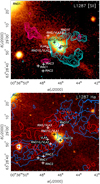 |
Fig. 3 Images of L1287 obtained with the CAHA 2.2 m telescope. The IR and centimeter continuum sources and their positions are identified with black and white crosses (depending on the light or dark background) Top: [SII] (color scale); the blue and red contours show the small-scale CO outflow observed by Juárez et al. (2019). Bottom: Hα (color scale);contours show the integrated line emission of NH3 (1, 1) from the blue and red filaments (this work). |
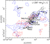 |
Fig. 4 NH3 (1, 1) integrated intensity map of the three velocity components in L1287. In order of increasing velocity: component 1 (Guitar core) − 20.16 to − 18.31 km s−1 (black contours andgray scale); component 2 (RNO 1 and blue filament) − 18.31 to − 17.07 km s−1 (blue contours); component 3 (red filament) − 17.07 to − 14.60 km s−1 (red contours). |
Guitar and filament parameters.
4 Discussion
4.1 Cluster of embedded YSOs near RNO 1B/1C
A small cluster of YSOs has been identified in the central part of L1287 from optical, IR, and radio observations. However, some uncertainties regarding the identification of the counterparts at different wavelengths and the number of distinct objects still remain. The VLA observations of Anglada et al. (1994) provide source positions at 3.6 cm with an accuracy of ~ 0.2″ and the observations of Quanz et al. (2007) provide mid-IR positions with an accuracy of ~ 0.3″. These two sets of observations unambiguously show that the young embedded object traced by IRAS 00338+6312 coincides with VLA 3 and is a different object than the FU Ori binary RNO 1B/1C. On the other hand, Anglada et al. (1994) tentatively associate the radio source VLA 1 with the FU Ori star RNO 1C. However, at that time the optical position of the star was known with an accuracy of only ~2″ (Staude & Neckel 1991; Weintraub & Kastner 1993), making the association uncertain. Now, after Gaia DR2 (Gaia Collaboration 2018) the optical positions of the two FU Ori stars, RNO 1B and 1C, are known to a precision of a fraction of mas, revealing that the positions of VLA 1 and RNO 1C differ by ~ 0.4″. Even though the positions are now much better constrained, the difference between radio and optical positions is only slightly greater than the accuracy of the VLA position (0.2″), and thus we consider that the association is still uncertain. The radio source VLA 2 falls within 0.4″ of the position of the mid-IR source RNO 1G (Quanz et al. 2007), so their positions are marginally consistent within the uncertainties. More accurate radio and IR positions are necessary for an unambiguous identification of these counterparts. The radio source VLA 4 has no known IR counterpart, but it seems to be associated with dust and compact molecular emission (Juárez et al. 2019).
Therefore, there are between 9 and 11 known independent objects (the Class 0/I objects IRAS–VLA 3, RNO 1G–VLA 2, IRAC 1, IRAC 2; the Class II objects RNO 1B, RNO 1C–VLA 1, RNO 1F, IRAC 3; and VLA 4), of which at least 8 are very likely YSOs, within a region of ~30″ (30 000 au = 0.15 pc in projection) toward the central part of L 1287.
The NH3 channel maps (Figs. A.1, A.2, and A.3) show a clumpy distribution of the emission, suggesting that different dense gas clumps, spatially and kinematically separated from each other, could be associated with the different YSOs of the proposed still-forming cluster (e.g., Quanz et al. 2007). The clumpy nature of the NH3 emission and possible association with the central young cluster is better seen in the − 18 km s−1 channel map of the NH3 (1, 1) main line shown in Fig. A.1, where a one-to-one association of ammonia clumps with IRAS–VLA 3, RNO 1B, and RNO 1C–VLA 1 is suggested. It is worth noting that the positions of the three ammonia clumps coincide with three of the dust cores recently reported by Juárez et al. (2019) from 1.3 mm SMA continuum observations. Juárez et al. (2019) identify in the central region of L1287 a total of 14 dust cores (some of them associated with molecular line emission), with masses of a fraction of solar mass, in their 1″ resolution SMA continuum observations (Juárez et al. 2019, see right panel of Fig. 1), inferring a very high degree of fragmentation in this central region. We also note that RNO 1F and IRAC 3 appear close to ammonia peaks in the − 18.6 and − 17.4 km s−1 channel maps, respectively, but their association with this dense gas is less clear.
This specific association between dust or molecular cores and YSOs is less clear in the images obtained after separating the NH3 emission in three components Some of the dust emission peaks might be just column density enhancements resulting from the superposition of several independent features along the line of sight instead of representingreal density enhancements in cores. It is also possible that some cores remain unidentified in NH3 because of the difficulties in fitting the different velocity components given the sensitivity, angular resolution, and spectral resolution of the present NH3 observations. We note that the positions of the sources IRAS–VLA 3, RNO 1B, RNO 1C–VLA 1, and RNO 1F fall toward the densest part of the Guitar core, and that the positions of RNO 1G–VLA 2 and VLA 4 fall near its southeast edge. However, there are no detectable signs of local heating or perturbation in the line width and rotational temperature maps toward these positions (Figs. 6 and 7). Therefore, unless the luminosity of these objects is insufficient to produce a detectable perturbation, we conclude that they are not associated with the Guitar core, which is likely observed in projection.
The role of IRAS–VLA3, the likely more embedded YSO and best candidate to drive the outflow, is particularly relevant. This source appears directly associated with NH3 emission from the red filament (see bottom panel of Fig. 5), and shows signs of dynamical perturbation traced by an increased line width (Fig. 6) and local heating (Figs. 7 and 8). However, because of the low spectral resolution and blending of line components, the interaction of IRAS–VLA 3 with dense gas remains still uncertain. New observations with higher angular and spectral resolution are necessary to clarify the role of this object with respect to the filaments.
The IR and radio sources appear to be distributed near the edges of the filaments. In particular, there is an apparent cavity, with a diameter of ~12 000 au toward the central region of the blue and red filaments, associated with Hα and [SII] emission. RNO 1C–VLA 1 is located at its center, and the sources IRAS–VLA 3, RNO 1B, RNO 1G–VLA2, VLA 4, and RNO 1F are located near its inner edge (see middle and lower panels in Figs. 5, 6, and 7, as well as the − 17.4 to − 16.6 km s−1 channel maps of Figs. A.1, A.2, and A.3). The presence of such a cavity in the L1287 core was proposed by Kenyon et al. (1993) from near-IR data, and by Yang et al. (1995) and McMuldroch et al. (1995) from CS data. Our Hα, [SII], and VLA ammonia observations provide a confirmation with data of higher quality. There are signs of dynamical perturbation and local heating, revealed by an increase in the NH3 line width and temperature in the blue filament near the positions of RNO 1G–VLA 2 and VLA 4 (middle panel in Fig. 6). RNO 1B appears projected toward the NH3 emission of the blue filament, with no clear signs of dynamical perturbation (Fig. 6), but with a hint of local heating (Figs. 7 and 8). The shape of the high-velocity CO outflow fits very well with the morphology of the cavity traced by the ammonia emission (Fig. 8), strongly supporting that this cavity has been created by the interaction of the outflow with the dense gas of the filaments (see further discussion in Sect. 4.3).
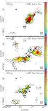 |
Fig. 5 L1287 NH3 beam-averaged column density, corrected for primary beam response, derived from NH3 (1, 1) and (2, 2), assuming a beam filling factor f = 1 (color scale).The color scale ranges from 2 × 1014 cm−2 (blue) to 2 × 1015 cm−2 (red). The contours are the NH3 (1, 1) integrated line intensity, corrected for opacity, AτmΔV, of the Guitar core (top, velocity range − 20.16 to − 18.31 km s−1), RNO 1 and blue filament (middle, − 18.31 to − 17.07 km s−1), and red filament (bottom, − 17.07 to − 14.60 km s−1). Contours are from 1 to 37 in steps of 4K km s−1. The crosses correspond to the YSOs identified in Fig. 3. |
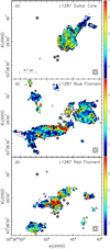 |
Fig. 6 L1287 NH3 hyperfine-line full width at half maximum, ΔV (color scale).The color scale ranges from 0.1 km s−1 (blue) to 1.0 km s−1 (red). The contours are the same as in Fig. 5. The crosses correspond to the YSOs identified in Fig. 3. |
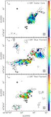 |
Fig. 7 L1287 rotational temperature, Trot, derived fromNH3 (1, 1) and (2, 2) (color scale). The color scale ranges from 10 K (blue) to 30 K (red). The contours are the same as in Fig. 5. The crosses correspond to the YSOs identified in Fig. 3. |
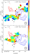 |
Fig. 8 Magnified image of the L1287 rotational temperature of the blue filament (top) and red filament (bottom), superimposed on the high-velocity CO emission (blue and red contours). There is a clear temperature increase at the walls of the cavity where the blue lobe of the outflow propagates. The crosses are the same as in Fig. 3. |
4.2 Guitar core
As already discussed, the Guitar core is probably seen in projection at the position of the embedded sources, and could be prestellar in nature. However, as we show in the following, there is a clear signpost of infall onto a central protostar, and thus the Guitar core is not prestellar but most probably a very young protostellar core.
The central velocity maps of the Guitar core (Fig. 9) show a spot of blueshifted gas at the center of the core (the sound hole of the guitar). This blueshifted gas is not produced by another clump of gas, with a blueshifted velocity, seen in projection at the center of the Guitar core, because the line width and rotational temperature of the gas of the Guitar core do not change significantly toward the blue spot (see Figs. 6 and 7). The variation in central velocity is smooth, with no abrupt changes, as can be seen in Figs. 9 and 10.
The blue spot can be interpreted as infalling gas toward the center of the clump (Anglada et al. 1991; Mayen-Gijon et al. 2014; Estalella et al. 2019). The model worked out by Anglada et al. (1987, 1991) and Estalella et al. (2019) assumes an infalling core with temperature and infall velocity that are power laws of the radial distance to the protostar, with a power-law index − 1∕2. In addition themodel assumes that the emission at any line-of-sight velocity is optically thick enough that the observer sees only the emission of the part of the isovelocity surface facing the observer. This produces an asymmetry in the emission, the emission from blueshifted channels being stronger than the corresponding redshifted channels.
This asymmetry produces a negative value of the first-order moment (intensity-averaged velocity) of the emission line, which can be calculated analytically for the case of an infinite angular resolution (Estalella et al. 2019). In order to model moment 1 observed with a finite angular resolution, the radial profile has to be convolved numerically with the beam of the observation. The model of Estalella et al. (2019) can also take into account the finite radius of the collapsing core. The model was used to fit the first-order moment maps of the NH3 (3, 3), (4, 4), (5, 5), and (6, 6) emission mapped with the VLA in the G31.41+0.31 hot molecular core, the H13 CO+ (J = 1–0) emission observed with Nobeyama, the 13CO (J = 2–1) emission observed with ALMA in the B335 core, and a preliminary analysis of the NH3 emission in L1287 presented here, deriving values of the central masses onto which the infall is taking place (Estalella et al. 2019).
In L1287 the (1, 1) and (2, 2) main component optical depths at the position of the blue spot were ~4 and ~2, respectively (see Fig. A.5), and therefore high enough to produce an asymmetry between the blueshifted and redshifted channels. The central velocity of the NH3 (1, 1) and (2, 2) lines for the Guitar core, obtained from the HfS fits, was averaged in rings 1″ wide, centered on the emission peak, up to a radius of 12″. The velocity profile obtained is shown in Fig. 10. The error bars are the rms dispersion of the velocities averaged in each ring. As can be seen in the figure, the velocity at the origin is blueshifted ~ 0.3 km s−1 with respect to the ambient gas velocity. The model of Estalella et al. (2019) predicts that such a velocity shift, observed with a beam of 3′′. 48 at a distance of 929 pc, can be produced by a central mass of ~ 2 M⊙. We fitted the infalling model with an infall radius much larger than the equivalent size of the beam (3200 au). The best-fit values for the central mass and systemic velocity were respectively M = 2.1 M⊙5 and Vsys = −18.67 km s−1. The quality of the fit is indicated by the value of the χ2 statistic for ν = 22 degrees of freedom (the total number of rings used in the fit, minus 2), χ2 = 11.4, which gives a reduced  . We checked the parameter space and found that χr < 0.9 for a range of masses, 1.1 < M < 3.4 M⊙, and of systemic velocities, − 18.81 < Vsys < −18.53 km s−1.
The conclusion is that the observed blue spot in the velocity map of the Guitar core is the hallmark of infalling motions onto a central object, and that a simple model to interpret the data predicts that a central mass of ~ 2M⊙ can explain the observed infalling motion.
 |
Fig. 9 Central velocity of NH3 (1, 1) (top) and (2, 2) (bottom) lines of the Guitar core in L1287 (color scale). The contours are the (1, 1) (top) and (2, 2) (bottom) integrated line emission. The velocity at the position of the emission peak is blueshifted ~ 0.3 km s−1 with respect to the rest of the gas of the core. This blue spot at the emission peak of the core (the sound hole of the guitar) is the hallmark of infalling material (see text). The crosses are the YSOs identified in Fig. 3. |
 |
Fig. 10 Ring-averaged central velocity of the NH3 (1, 1) (blue circles)and (2, 2) (red circles) lines in the Guitar core in L1287. The error bars are the rms of the values inside each ring. The central dashed line is the best fit of the infall hallmark model for a central mass of 2.1 M⊙, and the horizontal dotted line is the best-fit systemic velocity, Vsys = −18.67 km s−1. The fits for central masses of 1.1 and 3.4 M⊙ are also shown. |
4.3 Blue and red filaments
The blue and red filaments show clear signs of interaction with the embedded YSOs. In the region near the position of the sources the low velocity resolution of the data did not allow us to separate well the two velocity components, but significant line width and rotational temperature enhancements are seen for both filaments.
The interaction of the filaments with the star formation activity is clearly seen in Fig. 8, where we show in detail therotational temperature in the region of the filaments around the embedded YSOs, superimposed on a map of the outflow traced by high-velocity CO (2–1) observed by Juárez et al. (2019). Both filaments trace different parts of a cavity where the YSOs are located, and where the outflow propagates. The walls of this cavity is where the highest values of the gas temperature are found, indicating that the gas heating is probably due to the interaction of the high-velocity gas with the high-density ambient gas traced by the NH3 emission, as seen in other outflow cavity walls (e.g., IRAS 20293+3952, Palau et al. 2007).
Although both filaments are bent, some sections are almost straight and can be easily used to make a slice to analyze the structure of the filaments. The slice along the blue filament was at a position angle PA = −90°, and that along the red filament at PA = −42° (see Fig. 11). The half-width of the strip of pixels used in the analysis was 17″ (blue filament) and 23″ (red filament). The origin of offsets along the filaments was taken at the position of the intersection of the two slices, α(J2000) = 00h36m49.s30, δ(J2000) = +63°28′45.′′ 0. Position offsets increase westward (blue filament) and northwestward (red filament) from − 40″ to + 30″. The position of the cluster of embedded YSOs corresponds to a position offset of approximately + 20″ for both slices.
 |
Fig. 11 Slices used to analyze the filaments, superimposed on the integrated line intensity, corrected for opacity, Aτm ΔV, of the blue filament (blue contours) and the red filament (red contours). The origin of offsets along the filaments is taken at the position of the intersection of the two slices, and increase toward the west (blue filament) and the northwest (red filament) from − 40″ to + 30″. Ticks in the central line of the slices are at intervals of 10″. |
4.3.1 Velocity dispersion
In Fig. 12, we show a plot of the velocity dispersion for the slices of the blue and red filament. The increase in velocity dispersion is noticeable for positive offsets in both filaments, which correspond to the position near the cluster of embedded YSOs.
At a position offset of around zero there is also a sharp increase in line width of the blue filament. These positions correspond to the superposition of both filaments (the two slices cross at offset 0). The poor spectral resolution of the observationsmakes it difficult to disentangle the emission of the two filaments when they are superposed. This could be a factor that produces a spurious increase in the line width, due to the confusion of the emission of both filaments, or it could be a real effect caused by the mechanical interaction of the two filaments (see next section). Observations with a higher spectral resolution could help determine whether this increase in line width is real or not.
4.3.2 Gas temperature
The value of the kinetic temperature for the two slices of the blue and red filament is shown in Fig. 13. The kinetic temperature could only be derived for pixels of the slices with both NH3 (1, 1) and (2, 2) measurements. The median value of the kinetic temperature is low, Tk = 22.1 K for the blue filament and Tk = 22.9 K for the red filament, but significantly higher than the median temperature of the large-scale filament derived in the Hi-GAL catalogue, ~ 13.56 K (Schisano et al. 2020). In Fig. 14, we show the dust temperature map from Herschel (Juárez et al. 2019). In order to compare the gas and dust temperatures we computed from the Herschel data the dust temperature for a slice encompassing both filaments (see Fig. 14). As can be seen in Fig. 13, the dust temperature follows closely the variations in gas temperature, smoothed to the Herschel angular resolution (37″). This agreement shows that the gas and dust are closely coupled in L1287.
Two features are apparent. First, there is an increase in temperature around offset zero, at the crossing of the two filaments, indicating that the material of the two filaments are probably interacting with each other (i.e., the superposition of the filaments is real, and not only seen in projection). Second, there is a significant increase in temperature at positive offsets at ~ 20″, at the position of the cluster of embedded YSOs, suggesting gas heating caused by the interaction with the high-velocity gas of the outflows driven by IRAS–VLA 3 and by RNO 1C–VLA 1 (see Fig. 8). An alternative gas heating mechanism is radiative heating from the radiation of the embedded cluster. A simple application of the Stephan–Boltzmann law gives that an isotropic luminosity of ~ 20 L⊙ at a distance of 6000 au (the radius of the cavity) can produce a heating at the walls of the cavity up to a temperature of ~ 20 K. Thus, both mechanical and radiative heating could contribute to the observed gas temperature increase.
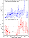 |
Fig. 12 NH3 velocity dispersion, |
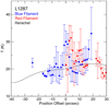 |
Fig. 13 Kinetic temperature derived from the NH3 data as a function of position along the blue filament (blue dots) and the red filament (red dots). Each data point is the median value of the kinetic temperature for points across the filament for a given position along the filament. The error bars indicate the median of the uncertainty. The dust temperature from Herschel data (Juárez et al. 2019) (beam size 37″), for a slice encompassing both filaments, is shown as a black solid line. |
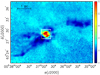 |
Fig. 14 Herschel large-scale map of the dust temperature (Juárez et al. 2019). A sharp temperature enhancement in the region mapped in NH3 (white box) is visible. The slanted black box indicates the slice used to compute the dust temperature from the Herschel data. |
4.3.3 Mach number
In order to characterize the importance of turbulence in the filaments, we estimated the median value of the Mach number,  , across the filament as a function of position along the filament. The Mach number is calculated as in Palau et al. (2015),
 (1)
(1)
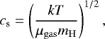
where cs is the isothermal sound speed,
 (2)
(2)
being k the Boltzmann constant, Tk the gas kinetic temperature, μgas = 2.3, the average molecular mass of the interstellar gas, mH the mass of the hydrogen atom, and σ3D,nth the 3D non-thermal velocity dispersion:
 (3)
(3)
The 1D non-thermal velocity dispersion, σ1D,nth, is given by the (squared) difference between observed and thermal velocity dispersion,
 (4)
(4)
with σ1D,obs given by the observed line full width at half maximum (deconvolved from the channel width), ΔV,
 (5)
(5)
and σth being the thermal line width,
 (6)
(6)
where  is the molecular mass of the NH3 molecule.
The results are shown in Fig. 15 as blue dots (blue filament) and red dots (red filament). The motion of the two filaments is nearly subsonic, except for the positions along the slices at positive offsets at ~ 10″ or 20″, at the position of the cluster of embedded YSOs, where the Mach number reaches values of ~ 2 (moderatelysupersonic) indicating the effect of the interaction with the high-velocity gas of the outflows driven by the IRAS source and RNO 1C. Alternatively, the higher Mach numbers near the cluster of YSOs could be indicative of ongoing infall from larger scales, consistent with theoretical models (e.g., Vázquez-Semadeni et al. 2019).
4.3.4 Mass per unit length
An important parameter of an elongated structure as a filament is its mass–density distribution, i.e., the mass per unit length. To compute this we used the column density determined for the pixels of the slices of the blue and red filaments. The mass per pixel spacing was obtained as the sum of the NH3 column density across the filament, for each position along the slice, converted to total mass using an NH3 abundance X(NH3) = 1 × 10⁻⁸, and divided by the size of the pixel in parsec. The results are shown in Fig. 16. The solid lines indicate the average value for the whole filament, Mlin = 61 M⊙ pc−1 (blue filament) and Mlin = 53M⊙ pc−1 (red filament) (see Table 2). The typical values (50% of the points) obtained for the blue filament are 30 M⊙ pc−1 ≤ Mlin ≤ 91M⊙ pc−1. The typicalvalues for the red filament are in general a bit lower, 18 M⊙ pc−1 ≤ Mlin ≤ 76 M⊙ pc−1.
The stability of a self-gravitating filament can be studied through the virial parameter, αv,
 (7)
(7)
where the critical value of the mass per unit length, Mlin,crit, for an infinite length cylinder is given by (see Appendix B)
 (8)
(8)
and is the mass per unit length whose self-gravitation is balanced by the thermal and non-thermal motions of the gas, given by the total velocity dispersion, σtot. The total velocity dispersion is evaluated as in Palau et al. (2015):
 (9)
(9)
For αv < 1 the cylinder cannot support its own mass against gravitation. It is collapsing or there are other mechanisms of support (e.g., magnetic field) not taken into account. Forαv > 1 the cylinder is expanding and will dissipate unless there are other mechanisms (external pressure) to confine its material.
The average values of σtot, Mlin,crit, and αv for the pixels of the slices of the blue and red filaments are given in Table 2. As can be seen from this analysis, both filaments are near virial equilibrium (αv = 0.7 for the blue filament and αv = 0.9 for the red filament). In other words, the mass that can be supported with the observed total velocity dispersion is similar to the mass per unit length observed for both filaments. However, this support must come from both thermal andnon-thermal motions, because the critical mass obtained from the thermal motions alone (i.e., using cs instead of σtot) is only ~ 40 M⊙ pc−1, below the observed values (Table 2).
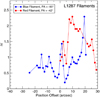 |
Fig. 15 Median value of the Mach number derived from the NH3 data as a function of position along the blue filament (blue dots) and the red filament (red dots). The slices used are the same as in Fig. 11. |
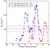 |
Fig. 16 Mass per unit length as a function of position along the blue filament (blue dots) and the red filament (red dots). The mass per unit length is obtained from the sum of NH3 column densities across the filament, for each position along the slice. The horizontal solid lines indicate the average value for the wholefilament, 61.2 M⊙ pc−1 (blue filament) and 53.0 M⊙ pc−1 (red filament). The dashed lines indicate the critical mass per unit length for thermal and non-thermal support,
|

Blue and red filament stability analysis.
4.3.5 Self-gravitating isothermal cylindrical filament model
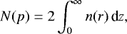
The self-gravitating isothermal cylindrical filament model (see Appendix B) predicts a column density as a function of distance from the filament axis, p, that is a power law with index − 3, flattened at the origin (see Eq. (B.11)). The model depends on two parameters only, the column density at the filament axis, N0, and the characteristic radius, h, a distance for which the column density is 0.35 times N0.
We obtained the H2 column density as afunction of distance to the filament axis for three positions of the blue filament and three other positions for the red filament, for which the column densities were estimated up to a distance ~ 0.03 pc. For larger distances the NH3 (1, 1) or (2, 2) emission was too faint to fit the spectra, and the column density could not be calculated. The results obtained are shown in Fig. 17. As can be seen, for the red filament the column density decreases with increasing distance. For the blue filament this behavior is not as clear, but we can see that in one position we were able to see a significant drop in column density with distance. The explanation for this could be that the blue filament is not a single entity, but there are hints of a substructure of subfilaments, or threads, that are not discernible with the present sensitivity, angular resolution, and spectral resolution of the NH3 observations. These subfilaments would be comparable to the velocity-coherent filamentary components (grouped into bundles) reported by Hacar et al. (2013, 2017), Shimajiri et al. (2019a), and Chen et al. (2020), which are typically separated about 0.2–0.9 km s−1.
We performed a least-squares fit of the isothermal cylindrical model to the column density as a function of the distance to the filament axis, up to a distance of ~0.03 pc, for both filaments. The parameters of the best-fit models are given in Table 3, and the models are also shown in Fig. 17. As can be seen, the fit is very good for the red filament, and fairly good for the blue filament. The models fitted for the blue and red filaments are very similar. The characteristic radii obtained are ~ 0.03 pc for both filaments. This value is different from the typical value of 0.1 pc found for Herschel filaments by Arzoumanian et al. (2011), but is consistent with the values found in the Integral Shaped Filament of Orion (Hacar et al. 2018) and in Serpens and Perseus (Dhabal et al. 2018). The volume density deduced from the model (Eq. (B.11)) is ~ 1 × 106 cm−3, and the mass per unit length predicted by the models is ~ 150M⊙ pc−1. The total velocity dispersion of the interstellar gas needed to have a stable isothermal filament (Eq. (8)) is ~ 0.58 km s−1. In general, we can say that the isothermal cylindrical model fits the observed column density as a function of distance to the filament axis.
We compared the column density obtained from the ammonia data and from the dust continuum emission from Herschel. The comparison can be seen in the bottom panel of Fig. 17, where we show the column density across the filament from the Herschel data (Juárez et al. 2019), and the sum of column densities of the isothermal cylindrical models for the blue and red filaments, convolved with the Herschel beam (FWHM = 37″). There is a clear agreement between the NH3 and Herschel data. This is indicative that the ammonia abundance used, X(NH3) = 1 × 10⁻⁸, is in agreement with the Herschel assumptions made in the data reduction (Juárez et al. 2019), and that we are detecting the bulk of the filament mass for distances upto p ≃ 0.03 pc from the filament axis.
However, there are discrepancies between the values obtained from the observations (see Table 2) and from the model (see Table 3) of the mass per unit length and the velocity dispersion. The apparent discrepancy in velocity dispersion can be explained by the fact that the NH3 observations are tracing small scales on the order of 0.03 pc (i.e., approximately the characteristic radius h), while the model takes into account the behavior of the gas on a large scale (up to an infinite distance from the filament axis). The velocity dispersion measured on large scales will be larger than the value measured on small scales from the NH3 emission. For instance, for the blue filament (see next section) we measure a velocity gradient across the filament of 11 km s−1 pc−1. This velocity gradient, measured at a scale of 0.15 pc (i.e., a diameter corresponding to a radius of only 2.5 times the characteristic radius h), would produce an increase in the velocity dispersion of 0.5 km s−1, making a total velocity dispersion of 0.6 km s−1, in agreement with the self-gravitating model.
Regarding the discrepancy in the mass per unit length, the column density obtained from the NH3 observations could only be integrated up to a distance approximately equal to the characteristic radius of the filaments, and the model predicts that the mass per unit length up to the characteristic radius h is half the total mass of the filament (see Appendix B). Thus, the discrepancy in the masses is smaller, although there is still a deficit of 16% in the measured mass of the blue filament, and of 37% in that of the red filament. This may be indicative that the NH3 observations were not able to recover all the mass of the filaments because we were not sensitive to the cold and low-density component of the gas of the filament, for which the NH3 (1, 1) or (2, 2) are not excited.
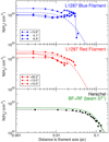 |
Fig. 17 Hydrogen column density as a function of distance to the filament axis, for three positions along the blue filament, at position offsets −6′′.5, −4′′.1, +10′′.9 (top panel), and along the red filament, at position offsets +10′′.0, +13′′.0, +20′′.2 (middle panel). The axes of the filaments are taken as the central lines of the slices used in Fig. 18. The blue and red dashed lines represent the self-gravitating isothermal filament models fitted for the blue and red filament data (see Table 3). The bottom panel shows the H2 column density from Herschel (Juárez et al. 2019) (black filled circles) and the self-gravitating isothermal filament model fit to the Herschel data (black dashed line). The green continuum line is the sumof the models for the blue and red filaments, convolved with the Herschel beam (FWHM = 37″). |
Isothermal filament model for the blue and red filaments.
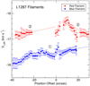 |
Fig. 18 Median of the central velocity of the NH3 (1, 1) line for points across the filament, as a function of position along the blue filament (blue dots) and the red filament (red dots). The two slices used are the same as in Fig. 11. The error bars indicate the median of the uncertainty of the values of the central velocity. The range of values is typically three times the median uncertainty. The dashed linesindicate the velocity gradients along the filaments. They are labeled “1” for the blue filament and “2” and “3” for the red filament. The same labels are used in Fig. 20. |
4.3.6 Central velocity: velocity gradients along and across the filaments
The (1, 1) central velocities for the slices of the blue and red filament are shown in Fig. 18. The blue filament, for position offsets between − 40″ and + 20″, shows an increasing velocity gradient of ~1.8 km s−1 pc−1 (labeled “1” in Fig. 18). For the red filament there is an increasing velocity gradient of ~ 2.1 km s−1 pc−1 for offsets from − 40″ to + 10″ (labeled “2”), and a decreasing velocity gradient of ~4.4 km s−1 pc−1 between offsets + 10″ and + 30″ (labeled “3”), encompassing the location of the cluster of YSOs, at an offset of + 20″. There is a hint of an oscillatory pattern in the velocity gradient seen along the blue filament, mainly around offsets − 20″ and 0″. These offsets are coincident with the position of cores embedded in the blue filament (see Fig. 11). Thus, these oscillations could originate from gas motions flowing toward the cores being formed within the filament, consistent with the model proposed byHacar & Tafalla (2011). Higher spectral resolution observations would definitely help establish the significance of such oscillations.
Figure 19 displays the central velocity map of the blue and red filaments. While the red filament does not show any clear velocity pattern, the blue filament shows a velocity gradient across its entire width, with a value of ~ 11 km s−1 pc−1, significantly larger than the velocity gradient observed along the filament. Evidence of such strong velocity gradients across the filaments has been found in other star-forming regions, for example Serpens South (Fernández-López et al. 2014; Dhabal et al. 2018), IRDC 18223 (Beuther et al. 2015), SDC 13 (Williams et al. 2018), and NGC 1333 (Dhabal et al. 2018). Interestingly, the clump located to the west of the main part of the blue filament also shows a velocity gradient across the filament axis of ~ 8 km s−1 pc−1, but in the opposite direction.
The observed velocity gradient of ~11 km s−1 pc−1 across the blue filament could result from a series of velocity-coherent subfilaments with slightly different velocities that overlap on the planeof the sky and are not resolved by our data. This is consistent with the flattened column density profile found for the blue filament (Fig. 17) and has been found in other filaments in the literature (Hacar et al. 2013, 2017; Shimajiri et al. 2019a).
Alternatively, the velocity gradient could be due to infalling material onto the filament, as has been claimed in other cases (Fernández-López et al. 2014; Gong et al. 2018; Shimajiri et al. 2019b; Chen et al. 2020). Although inSect. 4.3.5 we presented a model of a self-gravitating hydrostatic isothermal cylindrical filament, this is a very idealized case that does not take into account ingredients such as accretion onto the filament and further contraction. We consider here a contracting filament. In this scenario, the free-fall velocity andradius allow us to derive the free-fall time (Eq. (C.17)). For a velocity gradient of 11 km s−1 pc−1, a radius of the filament of 0.027 pc, and a mass per unit length of 61.2 M⊙ pc−1 (Table 2) the free-fall velocity is ~ 0.3 km s−1 and the free-fall time is ~0.05 Myr. This time has to be compared with the age of the filament. This can be estimated to be ~ 2 Myr, based on the evolutionary stage of the embedded YSOs, which range from a Class 0 object (IRAS–VLA 3) to a Class I/II object (FU Ori system RNO 1B/1C), and hence the age estimate from prestellar to Class 0 and Class II objects is ~ 0.6 Myr and 2 Myr, respectively (Evans et al. 2009). Thus, we can conclude that the accretion would take place on a timescale much shorter than the age of the filament, and hence the accretion scenario is compatible with the observed velocity gradient across the filament. We note that in Appendix C a cylindrical filament has been considered. However, in order to observe the velocity gradient across the filament, a slightly flattened filament would be required.
A second possible scenario that could produce the velocity gradient across the filaments is rotation (see, e.g., González Lobos & Stutz 2019). We used Eq. (1) of Recchi et al. (2014) to roughly estimate the contribution of rotational energy compared to gravity. It is worth emphasizing the approximate nature of the adopted energy balance as it does not include the effects of a radial density profile and the presence of internal temperature gradients. The observed velocity gradient corresponds to an angular velocity of ω ≃ 3.6 × 10⁻¹³ s−1. Adopting the mass per unit length and the characteristic radius given in Tables 2 and 3 (Mlin = 61.2M⊙ pc−1, Rc ≃ 0.027 pc), we obtained a ratio of rotation to gravitational energy, T∕W ≃ 0.17. This suggests that a rotation of the filament could explain the observed velocity gradient, with gravity being the dominant energy, but with a small contribution of the rotational energy that should be taken into consideration in the energy balance of the filament.
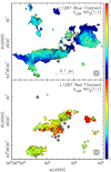 |
Fig. 19 Central velocity of the NH3 (1, 1) line of the L1287 blue and red filaments. The color scale for both panels ranges from − 18.5 km s−1 to − 17.1 km s−1. The contours are the (1, 1) integrated line intensity shown in Fig. 5. The crosses correspond to the YSOs identified in Fig. 3. |
4.4 Global scenario: Infall, inflow, and outflow in L1287
In Sect. 4.3.6, we analyzed the kinematics along the red and blue filaments. In particular, Fig. 18 revealed at least three distinct velocity gradients, two associated with the red filament and one associated with the blue filament. One possible interpretation for a velocity gradient along a filamentary structure is that it is tracing inflow motions toward a deep potential well. In the case of L1287 the potential well could be produced by the cluster of YSOs. This is consistent with simulations of the formation of filaments in molecular clouds that undergo collapse (e.g., Gómez & Vázquez-Semadeni 2014), and with previous observations of kinematics in filamentary structures in Serpens (Kirk et al. 2013; Lee et al. 2014; Gong et al. 2018; Dhabal et al. 2018), TMC 1 (Dobashi et al. 2019), several high-mass star-forming cores (Tackenberg et al. 2014; Lu et al. 2018), specific infrared dark clouds (SDC1: Peretto et al. 2014; G333: Veena et al. 2018; G22: Yuan et al. 2018; G14: Chen et al. 2019), Mon R2 (Treviño-Morales et al. 2019), Sgr B2 (Schwörer et al. 2019).
Assuming that this interpretation is correct, it is possible to build a 3D picture of the filamentary structures with respect to the observer, presented schematically in Fig. 20, where each filament portion associated with a velocity gradient is labeled (see Fig. 18). The increasing velocities observed along the filaments correspond to the velocity gradients 1 and 2 in Fig. 18. The bend in the red filament explains the change in the velocity gradient at position offset + 10″ from gradient 2 to 3. The embedded YSOs are located at position offset + 20″. The gap in the red filament is indicated as the part of the red filament sketched in white with a red contour. The Guitar core appears offset from the embedded YSOs because it is seen in projection at the position of the YSOs, but with no interaction with them, as discussed above. In this scenario, velocity gradients 2 and 3 correspond to the redshifted converging flow detected by Juárez et al. (2019) in DNC and other molecular tracers. Regarding the blueshifted converging flow reported in Juárez et al. (2019), this cannot be easily identified in our NH3 data, and it could instead result from material affected by the passage of the blueshifted lobe of the outflow driven by the IRAS source; alternatively, it could be material associated with the Guitar core, which is associated with the bluest NH3 gas found in the region. In the sketch we include the Guitar core, where infall has been detected (see Sect. 4.2). Therefore, the L1287 region at the center of the 10 pc filamentary structure seems to be associated with infall (Guitar core), inflow (blue and red filaments), and outflow (from the IRAS source especially) simultaneously. It seems that the different velocity filamentary structures identified from the NH3 emission converge at the location of the YSOs and thus our data strongly suggest that the cluster in L1287 is being formed at the intersection of filamentary structures where the inflow or infall of material is being funneled. This is fully consistent with the model of formation of clusters presented by Vázquez-Semadeni et al. (2017) and with a number of observational works (see, e.g., Jiménez-Serra et al. 2014), giving further support to a large-scale accretion scenario for the formation of stellar clusters.
 |
Fig. 20 Sketch of the velocity gradients along the blue and red filaments in L1287. The numbers 1, 2, and 3 identify the velocity gradients along the filaments shown in Fig. 18. The scale in arcsec corresponds to the position offset along the filaments of the same figure. |
5 Conclusions
We analyzed sensitive VLA D-configuration (beam ~3′′.5) observations of the (1, 1) and (2, 2) inversion transitions of ammonia, and optical Hα and [SII] emission in L1287. Our main conclusions are the following:
-
The [SII] emission, with a distribution similar to that of the Hα, shows a strong peak toward the position of RNO1. There is also strong [SII] emission coming from a compact (~10″, or ~9 000 au) region which encompasses the positions of the FU Ori binary RNO 1B/1C, while the positions of IRAS–VLA 3, RNO 1F, RNO 1G–VLA 2, and VLA 4 fall in the periphery where the emission is weaker. The [SII] emission is probably tracing the shocks at the base of the jet driving the molecular outflow.
-
The NH3 emission reveals a main elongated structure, centered near the positions of the FU Ori binary RNO 1B/1C and its associated still-forming cluster of YSOs. This ammonia structure extends over the observed field of view in the northwest–southeast direction, coinciding with the direction of the dust filament observed by Herschel and perpendicularly to the bipolar molecular outflow in the region. A secondary ammonia core is observed ~40″ (~0.17 pc) from the filaments, toward the position of RNO1 and near the edge of our field of view.
-
The NH3 emission is clumpy, with the channel map at − 18 km s−1 revealing three ammonia clumps apparently associated with the YSOs RNO 1B, RNO 2C–VLA 1, and IRAS–VLA 3. These ammonia clumps coincide with the positions of three of the 1.3 mm continuum dust clumps identified by Juárez et al. (2019), who infer a very high degree of fragmentation in this central region.
-
Three different velocity components were identified in the main ammonia structure. These components are referred to as the Guitar core, the blue filament (including the RNO1 core), and the red filament, in order of increasing velocity.
-
The Guitar core is compact (26″, 0.12 pc in diameter), has a mass of 30 M⊙, and shows no signs of interaction with the embedded YSOs traced by the IR, millimeter, or centimeter continuum. It is probablyseen in projection at the position of the YSOs. This core shows a clear central-blue-spot infall hallmark. The central velocity of the NH3 (1, 1) and (2, 2) lines is blueshifted 0.3 km s−1 with respect to the velocity of the core ambient gas. This compact blueshifted spot at the center of the core is interpreted as infall onto a central protostar of 2.1 M⊙.
-
The blueand red filaments are long (~1100″, 0.5 pc) and along the direction of the large-scale dust filament imaged by Herschel. The molecular filaments traced by NH3 have masses of 104 M⊙ (blue filament)and 13 M⊙ (red filament). The small-scale motions of the filament gas are nearly subsonic, except at the positions of the embedded YSOs.
-
The source VLA3 (IRAS 00338+6312), likely the most deeply embedded YSO and best candidate to drive the molecular outflow, appears directly associated with ammonia emission from the red filament, and with signs of dynamical perturbation, evidenced by an increased line width and local heating.
-
The ammonia images, after the velocity component associated with the Guitar core is removed, reveal a cavity with a diameterof ~12 000 au toward the central region of the blue and red filaments, with RNO 1C–VLA 1 located at its center and several other sources located near its inner wall. The existence of such a cavity had already been proposed, based on near-IR and CS data. The shape of the high-velocity CO outflow fits very well with the morphology of this cavity. The gas of the filaments shows a notable increase in velocity dispersion and rotational temperature at the interface between the outflow and the filaments at the cavity walls near the positions of some of the associated YSOs. These results suggest that the cavity was created by the interaction of the outflow with the dense gas of the filaments.
-
It was possible to estimate the column densities of the filaments up to a distance of ~0.03 pc from the filament axes. The column density across both filaments shows a marked decrease with distance to the filament axes. The mass per unit length of the filaments obtained from the integration of the observed column densities was ~60M⊙ pc−1. The fit with an isothermal cylindrical model gives a characteristic radius of 0.03 pc and a mass per unit length of ~150M⊙ pc−1. The isothermal model predicts a velocity dispersion higher than that measured on small scales (~0.03 pc), consistent with the measured velocity gradient across the filament, and the total mass per unit length of the filament approximately twice the mass up to the characteristic radius, consistent with our results.
-
The velocity gradient observed across the blue filament can be interpreted as infalling material onto the filament or as rotation. The velocity gradients along the filaments are interpreted as inflow motions toward the location of the embedded YSOs.
-
Additional ammonia observations with higher angular and spectral resolutions would be highly valuable to separate more clearly the three velocity components and better disentangle the kinematics and the role of the different embedded objects in the interaction between young stars, outflows, and dense gas in this region.
Acknowledgements
We thank Eugenio Schisano for providing us with the Herschel catalogue of the region. We thank the referee for his/her careful and helpful review of the paper. This work has been partially supported by the State Agency for Research (AEI) of the Spanish MCIU through the AYA2017-84390-C2 grant (cofunded with FEDER funds), and through the “Unit of Excellence María de Maeztu 2020-2023” award to the Institute of Cosmos Sciences (CEX2019-000918-M) and the ‘Center of Excellence Severo Ochoa’ award for the Instituto de Astrofísica de Andalucía (SEV-2017-0709). A. P. acknowledges financial support from CONACyT and UNAM-PAPIIT IN113119 grant, México.
Appendix A NH3 channel maps, spectra, and additional maps
In this appendix, we show additional maps obtained from the analysis of the NH3 (1, 1) and (2, 2) emission in L1287. The channel maps of the NH3 (1, 1) and (2, 2) line intensity, not corrected for primary beam response, are shown for the NH3 (1, 1) main line (Fig. A.1), NH3 (1, 1) inner-satellite line (Fig. A.2) and NH3 (2, 2) main line (Fig. A.3). The observed NH3 (1, 1) and (2, 2) spectra at the position of the embedded centimeter continuum and IR sources are shown in Fig. A.4. Finally, the NH3 (1, 1) and (2, 2) main line optical depths, τ1m and τ2m, are shown in Fig. A.5.
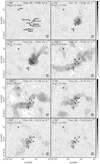 |
Fig. A.1 Channel maps of the NH3 (1, 1) main line intensity, not corrected for primary beam response. The contours are − 3, 3, 6, 9, 12, 15, 18, 23, and 28 times 0.5 K, the rms of the maps. The crosses correspond to the YSOs identified in Fig. 3 |
 |
Fig. A.2 Channel maps of the NH3 (1, 1) inner-satellite line intensity, not corrected for primary beam response. The contours are − 3, 3, 6, 9, 12, 15, 18, 23, and 28 times 0.5 K, the rms of the maps. The crosses correspond to the YSOs identified in Fig. 3 |
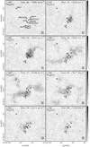 |
Fig. A.3 Channel maps of the NH3 (2, 2) main line intensity, not corrected for primary beam response. The contours are − 3, 3, 6, 9, 12,15, and 18 times 0.5 K, the rms of the maps. The crosses correspond to the YSOs identified in Fig. 3 |
 |
Fig. A.4 NH3 (1, 1) and (2, 2) spectra at the position of the embedded centimeter continuum and IR sources. |
 |
Fig. A.5 L1287 NH3 (1, 1) (left) and (2, 2) (right) main line optical depths, τ1m and τ2m. The color scale ranges from 0 to 6 for τ1m and from 0 to 2.5 for τ2m. The contours are the (1, 1) (left) and (2, 2) (right) integrated line intensities. The crosses correspond to the YSOs identified in Fig. 3. |
Appendix B Self-gravitating isothermal cylindrical filament model
The case of a self-gravitating isothermal cylindrical filament of infinite length was studied by Ostriker (1964) and used by Arzoumanian et al. (2011, 2013) in the analysis of filaments. The cylindrical filament is characterized by its mass density as a function of the distance to the cylinder axis, ρ(r), and by its temperature, T, assumed to be uniform. Ostriker (1964) derives an analytical solution for the equation of static equilibrium,with the boundary conditions imposed, i.e., the density at the cylinder axis is finite, ρ(0)= ρ0, and derivable, dρ∕dr(0) = 0. The solution can be written as
![\begin{equation*} \rho= \frac{\rho_0}{[1+(r/h)^2]^2}, \end{equation*}](/articles/aa/full_html/2020/12/aa37895-20/aa37895-20-eq14.png) (B.1)
(B.1)

and cs is the isothermal sound speed,
 (B.3)
(B.3)
with μgas being the mean molecular mass of the interstellar molecular gas, μgas = 2.3 for a 10% He abundance, and mH the mass of the hydrogen atom. This solution depends only on one free parameter, the density at the center of the cylinder, ρ0. The parameter h gives the characteristic radius of the filament, for which the density drops to ρ0 ∕4. The density given by this solution is flat at the center of the filament, and decreases sharply outward as a power law with a power-law index − 4,
 (B.4)
(B.4)
The mass per unit length of the filament, up to a radius r, Mlin(r), can be obtained by integration of the density,
 (B.5)
(B.5)
The total mass per unit length, Mlin ≡ Mlin(r →∞), remains finite,
 (B.6)
(B.6)
and depends only on the temperature of the gas (through the value of cs). One-half of the total mass is within a radius r = h,
 (B.7)
(B.7)
The relation between the mass density of the gas, ρ, and the molecular hydrogen number density, n, is given by
 (B.8)
(B.8)
where  is the mean molecular gas per hydrogen molecule,
  for a 10% He abundance.
When the filament is observed perpendicularly, i.e., when the line of sight is perpendicular to the cylinder axis, the column density will depend only on the projected radial distance from the filament axis, p, and will be
 (B.9)
(B.9)
where z is the coordinate along the line of sight, and p2 + z2 = r2. By changing the integration variable from z to r, with  , we obtain
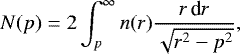 (B.10)
which is the standard form of the Abel Transform of n(r) (Bracewell 2000). The integral can be calculated analytically, and the result is
 (B.11)
The column density of the isothermal cylindrical filament is flat at the center of the filament, and decreases outward as a power law with a power-law index of − 3:
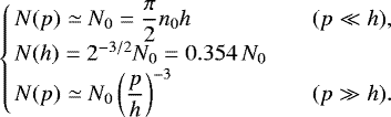 (B.12)
The model depends on two parameters that can be fitted to the observational data: N0, the column density at the filament axis, and h, the characteristic radius of the filament. The expressions of the other physical parameters of the filament can be obtained from N0 and h. The expressions for the gas temperature, T; the total mass per unit length, Mlin; and the number density at the filament axis, n0, are
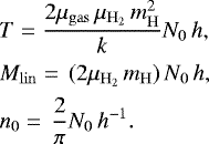 (B.13)
In practical units, the expressions become
![\begin{align*} &\left[\frac{T}{\mathrm{K}}\right] = 2.69 \left[\frac{N_0}{10^{20}\ \mathrm{cm^{-2}}}\right] \left[\frac{h}{\mathrm{pc}}\right],\nonumber\\ &\left[\frac{M_{\mathrm{lin}}}{M_{\odot}\mathrm{~pc}^{-1}}\right] = 4.49 \left[\frac{N_0}{10^{20}\ \mathrm{cm^{-2}}}\right] \left[\frac{h}{\mathrm{pc}}\right],\\ &\left[\frac{n_0}{\mathrm{cm^{-3}}}\right] = 20.6 \left[\frac{N_0}{10^{20}\ \mathrm{cm^{-2}}}\right] \left[\frac{h}{\mathrm{pc}}\right]^{-1}.\nonumber \end{align*}](/articles/aa/full_html/2020/12/aa37895-20/aa37895-20-eq30.png) (B.14)
(B.14)
Appendix C Free-fall of a cylindrical filament
The free-fall of a cylindrical filament of infinite length was studied by Penston (1969), among others, while the more general case of a finite length filament has also been the object of several studies (see, e.g., Pon et al. 2012, and references therein). In the following we summarize the results of Penston (1969), and give the expressions used to analyze the filaments in L1287.
For a cylindrical mass distribution the gravitational field is radial (perpendicular to the cylinder axis). The gravitational acceleration is
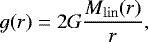 (C.1)
(C.1)
where Mlin(r) is the mass per unit length of the cylinder, inside a radius r. The mass for radii greater than the distance r to the axis does not contribute to the gravitational force. The former expression can be written as a differential equation in the radial velocity v,
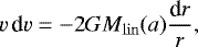 (C.2)
(C.2)
where Mlin(a) is the mass per length unit at the initialradius of the free fall, a, a value of the mass that is constant during the free fall. The integration of the differential equation from the initial radius, a, with zero initial velocity gives
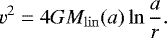 (C.3)
(C.3)
It is useful to define the characteristic velocity, vc ( times the Keplerian orbital velocity),
 (C.4)
(C.4)
This is a differential equation in the radius r(t),
 (C.6)
(C.6)
whose integration, with the initial condition r(0) = a, can be given as
 (C.7)
(C.7)
By using the adimensional parameter θ (Penston 1969),
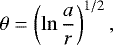 (C.8)
(C.8)
the integral of Eq. (C.7) results in
 (C.9)
(C.9)
where erf is the error function. The free-fall time, tff, is obtained for r → 0, implying θ →∞ (Eq. (C.8)), so that erf θ → 1, and Eq. (C.9) gives
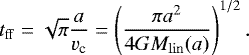 (C.10)
In summary, the equations of the collapse can be written as a function of the parameter θ, which varies from 0 (beginning of the collapse, r = a) to ∞ (end of the collapse, r → 0),
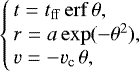 (C.11)
where a is the initial radius, vc is given by Eq. (C.4), and tff by Eq. (C.10). In practical units, the characteristic velocity vc (Eq. (C.4)) is given by
![\begin{equation*}\left[\frac{v_{\textrm{c}}}{\mathrm{km~s^{-1}}}\right] = 0.131 \left[\frac{M_{\mathrm{lin}}(a)}{M_{\odot}\mathrm{~pc}^{-1}}\right]^{1/2}, \end{equation*}](/articles/aa/full_html/2020/12/aa37895-20/aa37895-20-eq43.png) (C.12)
(C.12)
and the free-fall time from an initial radius a (Eq. (C.10)) is
![\begin{equation*}\left[\frac{t_{\mathrm{ff}}}{\mathrm{Myr}}\right] = 13.2 \left[\frac{a}{\mathrm{pc}}\right] \left[\frac{M_{\mathrm{lin}}(a)}{M_{\odot}\mathrm{~pc}^{-1}}\right]^{-1/2} .\end{equation*}](/articles/aa/full_html/2020/12/aa37895-20/aa37895-20-eq44.png) (C.13)
(C.13)
Let us now assume that we observe a free-fall velocity v at a distancer from the filament axis, and we want to know from which radius, a, the free-fall initiated, and the free-fall time. In addition, let us assume that the radius of observation r is r ≫ h (i.e., the infall velocity is observed far enough from the filament axis), so that Mlin(a) is a good approximation to the total mass of the filament Mlin. By using Eq. (C.11), the initial radius of the infall is
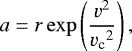 (C.14)
which allows us to check whether a ≫ h, as assumed. The total free-fall time from the initial radius a is
 (C.15)
In practical units, the initial radius a (Eqs. (C.12), (C.4)) is given by
![\begin{equation*}\left[\frac{a}{\mathrm{pc}}\right] = \left[\frac{r}{\mathrm{pc}}\right] \exp\left( 58.1 \left[\frac{v}{\mathrm{km~s^{-1}}}\right]^2 \left[\frac{M_{\mathrm{lin}}}{M_{\odot}\mathrm{~pc}^{-1}}\right]^{-1} \right), \end{equation*}](/articles/aa/full_html/2020/12/aa37895-20/aa37895-20-eq47.png) (C.16)
(C.16)
and the total free-fall time tff (Eqs. (C.13), (C.4)) is
![\begin{eqnarray*}\left[\frac{t_{\mathrm{ff}}}{\mathrm{Myr}}\right] & = & 13.2 \left[\frac{r}{\mathrm{pc}}\right] \left[\frac{M_{\mathrm{lin}}}{M_{\odot}\mathrm{~pc}^{-1}}\right]^{-1/2} \nonumber\\ && \times\exp\left( 58.1 \left[\frac{v}{\mathrm{km~s^{-1}}}\right]^2 \left[\frac{M_{\mathrm{lin}}}{M_{\odot}\mathrm{~pc}^{-1}}\right]^{-1} \right). \end{eqnarray*}](/articles/aa/full_html/2020/12/aa37895-20/aa37895-20-eq48.png) (C.17)
(C.17)
References
- André, P., Men’shchikov, A., Bontemps, S., et al. 2010, A&A, 518, A102 [Google Scholar]
- Anglada, G., Rodríguez, L. F., Cantó, J., Estalella, R., & López, R. 1987, A&A, 186, 280 [NASA ADS] [Google Scholar]
- Anglada, G., Estalella, R., Rodríguez, L. F., Cantó, J., & López, R. 1991, A&A, 252, 639 [NASA ADS] [Google Scholar]
- Anglada, G., Rodríguez, L. F., Girart, J. M., Estalella, R., & Torrelles, J. M. 1994, ApJ, 420, L91 [NASA ADS] [CrossRef] [Google Scholar]
- Arzoumanian, D., André, Ph., Didelon, P., et al. 2011, A&A, 529, A6 [NASA ADS] [CrossRef] [EDP Sciences] [Google Scholar]
- Arzoumanian, D., André, Ph., Peretto, N., & Könyves, V. 2013, A&A, 553, A119 [NASA ADS] [CrossRef] [EDP Sciences] [Google Scholar]
- Beuther, H., Ragan, S. E., Johnstone, K., et al. 2015, A&A, 584, A67 [NASA ADS] [CrossRef] [EDP Sciences] [Google Scholar]
- Bracewell, R. N. 2000, The Fourier Transform and its Applications, 3rd ed. (Boston: McGraw-Hill Higher Education) [Google Scholar]
- Chen, H.-R. V., Zhang, Q., Wright, M. C. H., et al. 2019, ApJ, 875, 24 [NASA ADS] [CrossRef] [Google Scholar]
- Chen, C.-Y., Mundy, L. G., Ostriker, E. C., Storm, S., Dhabal, A. 2020, MNRAS, 494, 3675 [CrossRef] [Google Scholar]
- Connelley, M. S., Reipurth, B., & Tokunaga, A. T. 2007, AJ, 133, 1528 [NASA ADS] [CrossRef] [Google Scholar]
- Dhabal, A., Mundy, L. G., Rizzo, M. J., Storm, S., & Teuben, P. 2018, ApJ, 853, 169 [NASA ADS] [CrossRef] [Google Scholar]
- Dobashi, K., Shimoikura, T., Ochiai, T., et al. 2019, ApJ, 879, 88 [CrossRef] [Google Scholar]
- Estalella, R. 2017, PASP, 129, 025003 [NASA ADS] [CrossRef] [Google Scholar]
- Estalella, R., Mausberger, R., Torrelles, J. M., et al. 1993, ApJ, 419, 698 [NASA ADS] [CrossRef] [Google Scholar]
- Estalella, R., Anglada, G., Díaz-Rodríguez, A. K., & Mayen-Gijon; J. M. 2019, A&A, 626, A84 [NASA ADS] [CrossRef] [EDP Sciences] [Google Scholar]
- Evans, II, N. J., Dunham, M. M., Jørgensen, J. K., et al. 2009, ApJS, 181, 321 [NASA ADS] [CrossRef] [Google Scholar]
- Fehér, O., Kóspál, Á., Ábrahám, P., Hogerheijde, M. R., & Brinch, C. 2017, A&A, 607, A39 [NASA ADS] [CrossRef] [EDP Sciences] [Google Scholar]
- Fernández-López, M., Arce, H. G., Looney, L., et al. 2014, ApJ, 790, L19 [NASA ADS] [CrossRef] [Google Scholar]
- Fiebig, D. 1995, A&A, 298, 207 [NASA ADS] [Google Scholar]
- Fiebig, D. 1997, A&A, 327, 758 [NASA ADS] [Google Scholar]
- Friesen, R. K., Pineda, J. E., Rosolowsky, E., et al. 2017, ApJ, 843, 63 [NASA ADS] [CrossRef] [Google Scholar]
- Gaia Collaboration (Brown, A. G. A., et al.) 2018, A&A, 616, A1 [NASA ADS] [CrossRef] [EDP Sciences] [Google Scholar]
- Gómez, G. C., & Vázquez-Semadeni, E. 2014, ApJ, 791, 124 [NASA ADS] [CrossRef] [Google Scholar]
- Gong, Y., Li, G. X., Mao, R. Q., et al. 2018, A&A, 620, A62 [NASA ADS] [CrossRef] [EDP Sciences] [Google Scholar]
- González Lobos, V., & Stutz, A. M. 2019, MNRAS, 489, 4771 [CrossRef] [Google Scholar]
- Hacar, A., & Tafalla, M. 2011, A&A, 533, A34 [NASA ADS] [CrossRef] [EDP Sciences] [Google Scholar]
- Hacar, A., Tafalla, M., Kauffmann, J., et al. 2013, A&A, 554, A55 [NASA ADS] [CrossRef] [EDP Sciences] [Google Scholar]
- Hacar, A., Tafalla, M., & Alves, J. 2017, A, 606, A123 [Google Scholar]
- Hacar, A., Tafalla, M., Forbrich, J., et al. 2018, A&A, 610, A77 [NASA ADS] [CrossRef] [EDP Sciences] [Google Scholar]
- Jiménez-Serra, I., Caselli, P., Fontani, F., et al. 2014, MNRAS, 439, 1996 [NASA ADS] [CrossRef] [Google Scholar]
- Juárez, C., Liu, H. B., Girart, J. M., et al. 2019, A&A, 621, A140 [NASA ADS] [CrossRef] [EDP Sciences] [Google Scholar]
- Kenyon, S. J., Hartmann, L., Gómez, M., Carr, J. S., & Tokunaga, A. 1993, AJ, 105, 1505 [NASA ADS] [CrossRef] [Google Scholar]
- Kirk, H., Myers, P. C., Bourke, T. L., et al. 2013, ApJ, 766, 115 [NASA ADS] [CrossRef] [Google Scholar]
- Könyves, V., André, P., Men’shchikov, A., et al. 2015, A&A, 584, A91 [NASA ADS] [CrossRef] [EDP Sciences] [Google Scholar]
- Krumholz, M. R., Burkhart, B., Forbes, J. C., & Crocker, R. M. 2018, MNRAS, 477, 2716 [NASA ADS] [CrossRef] [Google Scholar]
- Lee, K. I., Fernández-López, M., Storm, S., et al. 2014, ApJ, 797, 76 [NASA ADS] [CrossRef] [Google Scholar]
- López, R., Riera, A., Estalella, R., & Gómez, G. 2020, A&A, submitted [Google Scholar]
- Lu, X., Zhang, Q., Liu, H. B., et al. 2018, ApJ, 855, 9 [NASA ADS] [CrossRef] [Google Scholar]
- Mayen-Gijon, J. M., Anglada, G., Osorio, M., et al. 2014, MNRAS, 437, 3766 [NASA ADS] [CrossRef] [Google Scholar]
- McMuldroch, S., Blake, G. A., & Sargent, A. I. 1995, AJ, 110, 354 [NASA ADS] [CrossRef] [Google Scholar]
- Molinari, S., Swinyard, B., Bally, J., et al. 2010, A&A, 518, A100 [Google Scholar]
- Myers, P. C. 2009, ApJ, 700, 1609 [NASA ADS] [CrossRef] [EDP Sciences] [Google Scholar]
- Ostriker, J. 1964, ApJ, 140, 1056 [NASA ADS] [CrossRef] [MathSciNet] [Google Scholar]
- Palau, A., Estalella, R., Girart, J. M., et al. 2007, A&A, 465, 219 [NASA ADS] [CrossRef] [EDP Sciences] [Google Scholar]
- Palau, A., Ballesteros-Paredes, J., Vázquez-Semadeni, E., et al. 2015, MNRAS, 453, 3785. [NASA ADS] [CrossRef] [Google Scholar]
- Pension, M. V. 1969, MNRAS, 144, 425 [NASA ADS] [CrossRef] [Google Scholar]
- Peretto, N., Fuller, G. A., André, Ph., et al. 2014, A&A, 561, A83 [NASA ADS] [CrossRef] [EDP Sciences] [Google Scholar]
- Polychroni, D., Schisano, E., Elia, D., et al. 2013, ApJ, 777, L33 [NASA ADS] [CrossRef] [Google Scholar]
- Pon, A., Toal, J. A. Johnstone, D., et al. 2012, ApJ, 756, 145 [NASA ADS] [CrossRef] [Google Scholar]
- Quanz, S. P., Henning, T., Bouwman, J., Linz, H., & Lahuis, F. 2007, ApJ, 658, 487 [NASA ADS] [CrossRef] [Google Scholar]
- Recchi, S., Hacar, A., & Palestini, A. 2014, MNRAS, 444, 1775 [NASA ADS] [CrossRef] [Google Scholar]
- Rygl, K. L. J., Brunthaler, A., Reid, M. J., et al. 2010, A&A, 511, A2 [NASA ADS] [CrossRef] [EDP Sciences] [Google Scholar]
- Sandell, G., & Weintraub, D. A. 2001, ApJS, 134, 115 [NASA ADS] [CrossRef] [Google Scholar]
- Schisano, E., Molinari, S., Elia, D., et al. 2020, MNRAS, 492, 5420 [NASA ADS] [CrossRef] [Google Scholar]
- Schwörer, A., Sánchez-Monge, Á., Schilke, P., et al. 2019, A&A, 628, A6 [NASA ADS] [CrossRef] [EDP Sciences] [Google Scholar]
- Sepúlveda, I. 2001, PhD Thesis, University of Barcelona, Spain [Google Scholar]
- Sepúlveda, I., Anglada, G., Estalella, R., et al. 2011, A&A, 527, A41 [NASA ADS] [CrossRef] [EDP Sciences] [Google Scholar]
- Skinner, S. L., & Güdel, M. 2020, AJ, 159, 221 [CrossRef] [Google Scholar]
- Shimajiri, Y., André, Ph., Ntormousi, E., et al. 2019a, A&A, 632, A83 [NASA ADS] [CrossRef] [EDP Sciences] [Google Scholar]
- Shimajiri, Y., André, Ph., Palmeirim, P., et al. 2019b, A&A, 623, A16 [NASA ADS] [CrossRef] [EDP Sciences] [Google Scholar]
- Snell, R. L., Dickman, R. L., & Huang, Y. L. 1990, ApJ, 352, 139 [NASA ADS] [CrossRef] [Google Scholar]
- Staude, H. J., & Neckel, Th. 1991, A&A, 244, L13 [Google Scholar]
- Stutz, A. M., & Kainulainen, J. 2015, A&A, 577, A6 [NASA ADS] [CrossRef] [EDP Sciences] [Google Scholar]
- Tackenberg, J., Beuther, H., Henning, Th., et al. 2014, A&A, 565, A101 [NASA ADS] [CrossRef] [EDP Sciences] [Google Scholar]
- Treviño-Morales, S. P., Fuente, A., Sánchez-Monge, Á., et al. 2019, A&A, 629, A81 [NASA ADS] [CrossRef] [EDP Sciences] [Google Scholar]
- Umemoto, T., Saito, M., Yang, J., & Hirano, N. 1999, in Star Formation 1999, ed. T. Nakamoto, 227 [Google Scholar]
- Vázquez-Semadeni, E., González-Samaniego, A., Colín, P. 2017, MNRAS, 467, 1313 [Google Scholar]
- Vázquez-Semadeni, E., Palau, A., Ballesteros-Paredes, J., Gómez, G. C., Zamora-Avilés, M. 2019, MNRAS, 490, 3061 [NASA ADS] [CrossRef] [Google Scholar]
- Veena, V. S., Vig, S., Mookerjea, B., et al. 2018, ApJ, 852, 93 [NASA ADS] [CrossRef] [Google Scholar]
- Weintraub, D. A., & Kastner, J. 1993, ApJ, 411, 767 [NASA ADS] [CrossRef] [Google Scholar]
- Williams, G. M., Peretto, N., Avison, A., Duarte-Cabral, A., Fuller, G. A. 2018, A&A, 613, A11 [NASA ADS] [CrossRef] [EDP Sciences] [Google Scholar]
- Xu, J.-L., Li, D., Zhang, C.-P., et al. 2016, ApJ, 819, 117 [NASA ADS] [CrossRef] [Google Scholar]
- Yang, J., Umemoto, T., Iwata, T., & Fukui, Y. 1991, ApJ, 373, 137 [NASA ADS] [CrossRef] [Google Scholar]
- Yang, J., Ohashi, N., & Fukui, Y. 1995, ApJ, 455, 175 [NASA ADS] [CrossRef] [Google Scholar]
- Yuan, J., Li, J.-Z., Wu, Y., et al. 2018, ApJ, 852, 12 [NASA ADS] [CrossRef] [Google Scholar]
In Estalella et al. (2019), because of a bug in the plotting program used, the ring-averaged velocities were fitted up to radial distances of 20″, well outside of the central part of the core. The correct central mass for L1287 is the value given in the present paper. The correction does not affect values of the central mass for other cores in Estalella et al. (2019).
All Tables
All Figures
|
Fig. 1 Herschel large-scale map (left) of H2 column density (Juárez et al. 2019). The large-scale filament, roughly in the southeast–northwest direction, can be clearly seen. The large box shows the region mapped in NH3, encompassing the area of highest column density of the filament. The embedded sources detected in the IR, millimeter, and centimeter continuum are identified in the enlarged view (right) of the small box in the central area (except RNO 1, which lies outside the small box). The black dots (•) in the right panel correspond to millimeter dust-continuum emission (Juárez et al. 2019), and the plus signs (+) to mid-IR sources (Quanz et al. 2007) and centimeter continuum sources (Anglada et al. 1994). |
| In the text | |
|
Fig. 2 Examples of NH3 (1, 1) (left) and (2, 2) (right) spectra in L1287: observed (black), fitted component 1 (green), component 2 (blue), component 3 (red). The dotted vertical lines show the range of velocities used for fitting the three velocity components. From top to bottom: position A, component 1 only; B, component 2 only; C, component 3 only; D, components 1 and 3; E, components 2 and 3; F, all three components present. The coordinates of the six positions are given in the right panels. |
| In the text | |
|
Fig. 3 Images of L1287 obtained with the CAHA 2.2 m telescope. The IR and centimeter continuum sources and their positions are identified with black and white crosses (depending on the light or dark background) Top: [SII] (color scale); the blue and red contours show the small-scale CO outflow observed by Juárez et al. (2019). Bottom: Hα (color scale);contours show the integrated line emission of NH3 (1, 1) from the blue and red filaments (this work). |
| In the text | |
|
Fig. 4 NH3 (1, 1) integrated intensity map of the three velocity components in L1287. In order of increasing velocity: component 1 (Guitar core) − 20.16 to − 18.31 km s−1 (black contours andgray scale); component 2 (RNO 1 and blue filament) − 18.31 to − 17.07 km s−1 (blue contours); component 3 (red filament) − 17.07 to − 14.60 km s−1 (red contours). |
| In the text | |
|
Fig. 5 L1287 NH3 beam-averaged column density, corrected for primary beam response, derived from NH3 (1, 1) and (2, 2), assuming a beam filling factor f = 1 (color scale).The color scale ranges from 2 × 1014 cm−2 (blue) to 2 × 1015 cm−2 (red). The contours are the NH3 (1, 1) integrated line intensity, corrected for opacity, AτmΔV, of the Guitar core (top, velocity range − 20.16 to − 18.31 km s−1), RNO 1 and blue filament (middle, − 18.31 to − 17.07 km s−1), and red filament (bottom, − 17.07 to − 14.60 km s−1). Contours are from 1 to 37 in steps of 4K km s−1. The crosses correspond to the YSOs identified in Fig. 3. |
| In the text | |
|
Fig. 6 L1287 NH3 hyperfine-line full width at half maximum, ΔV (color scale).The color scale ranges from 0.1 km s−1 (blue) to 1.0 km s−1 (red). The contours are the same as in Fig. 5. The crosses correspond to the YSOs identified in Fig. 3. |
| In the text | |
|
Fig. 7 L1287 rotational temperature, Trot, derived fromNH3 (1, 1) and (2, 2) (color scale). The color scale ranges from 10 K (blue) to 30 K (red). The contours are the same as in Fig. 5. The crosses correspond to the YSOs identified in Fig. 3. |
| In the text | |
|
Fig. 8 Magnified image of the L1287 rotational temperature of the blue filament (top) and red filament (bottom), superimposed on the high-velocity CO emission (blue and red contours). There is a clear temperature increase at the walls of the cavity where the blue lobe of the outflow propagates. The crosses are the same as in Fig. 3. |
| In the text | |
|
Fig. 9 Central velocity of NH3 (1, 1) (top) and (2, 2) (bottom) lines of the Guitar core in L1287 (color scale). The contours are the (1, 1) (top) and (2, 2) (bottom) integrated line emission. The velocity at the position of the emission peak is blueshifted ~ 0.3 km s−1 with respect to the rest of the gas of the core. This blue spot at the emission peak of the core (the sound hole of the guitar) is the hallmark of infalling material (see text). The crosses are the YSOs identified in Fig. 3. |
| In the text | |
|
Fig. 10 Ring-averaged central velocity of the NH3 (1, 1) (blue circles)and (2, 2) (red circles) lines in the Guitar core in L1287. The error bars are the rms of the values inside each ring. The central dashed line is the best fit of the infall hallmark model for a central mass of 2.1 M⊙, and the horizontal dotted line is the best-fit systemic velocity, Vsys = −18.67 km s−1. The fits for central masses of 1.1 and 3.4 M⊙ are also shown. |
| In the text | |
|
Fig. 11 Slices used to analyze the filaments, superimposed on the integrated line intensity, corrected for opacity, Aτm ΔV, of the blue filament (blue contours) and the red filament (red contours). The origin of offsets along the filaments is taken at the position of the intersection of the two slices, and increase toward the west (blue filament) and the northwest (red filament) from − 40″ to + 30″. Ticks in the central line of the slices are at intervals of 10″. |
| In the text | |
|
Fig. 12 NH3 velocity dispersion, |
| In the text | |
|
Fig. 13 Kinetic temperature derived from the NH3 data as a function of position along the blue filament (blue dots) and the red filament (red dots). Each data point is the median value of the kinetic temperature for points across the filament for a given position along the filament. The error bars indicate the median of the uncertainty. The dust temperature from Herschel data (Juárez et al. 2019) (beam size 37″), for a slice encompassing both filaments, is shown as a black solid line. |
| In the text | |
|
Fig. 14 Herschel large-scale map of the dust temperature (Juárez et al. 2019). A sharp temperature enhancement in the region mapped in NH3 (white box) is visible. The slanted black box indicates the slice used to compute the dust temperature from the Herschel data. |
| In the text | |
|
Fig. 15 Median value of the Mach number derived from the NH3 data as a function of position along the blue filament (blue dots) and the red filament (red dots). The slices used are the same as in Fig. 11. |
| In the text | |
|
Fig. 16 Mass per unit length as a function of position along the blue filament (blue dots) and the red filament (red dots). The mass per unit length is obtained from the sum of NH3 column densities across the filament, for each position along the slice. The horizontal solid lines indicate the average value for the wholefilament, 61.2 M⊙ pc−1 (blue filament) and 53.0 M⊙ pc−1 (red filament). The dashed lines indicate the critical mass per unit length for thermal and non-thermal support,
|
| In the text | |
|
Fig. 17 Hydrogen column density as a function of distance to the filament axis, for three positions along the blue filament, at position offsets −6′′.5, −4′′.1, +10′′.9 (top panel), and along the red filament, at position offsets +10′′.0, +13′′.0, +20′′.2 (middle panel). The axes of the filaments are taken as the central lines of the slices used in Fig. 18. The blue and red dashed lines represent the self-gravitating isothermal filament models fitted for the blue and red filament data (see Table 3). The bottom panel shows the H2 column density from Herschel (Juárez et al. 2019) (black filled circles) and the self-gravitating isothermal filament model fit to the Herschel data (black dashed line). The green continuum line is the sumof the models for the blue and red filaments, convolved with the Herschel beam (FWHM = 37″). |
| In the text | |
|
Fig. 18 Median of the central velocity of the NH3 (1, 1) line for points across the filament, as a function of position along the blue filament (blue dots) and the red filament (red dots). The two slices used are the same as in Fig. 11. The error bars indicate the median of the uncertainty of the values of the central velocity. The range of values is typically three times the median uncertainty. The dashed linesindicate the velocity gradients along the filaments. They are labeled “1” for the blue filament and “2” and “3” for the red filament. The same labels are used in Fig. 20. |
| In the text | |
|
Fig. 19 Central velocity of the NH3 (1, 1) line of the L1287 blue and red filaments. The color scale for both panels ranges from − 18.5 km s−1 to − 17.1 km s−1. The contours are the (1, 1) integrated line intensity shown in Fig. 5. The crosses correspond to the YSOs identified in Fig. 3. |
| In the text | |
|
Fig. 20 Sketch of the velocity gradients along the blue and red filaments in L1287. The numbers 1, 2, and 3 identify the velocity gradients along the filaments shown in Fig. 18. The scale in arcsec corresponds to the position offset along the filaments of the same figure. |
| In the text | |
|
Fig. A.1 Channel maps of the NH3 (1, 1) main line intensity, not corrected for primary beam response. The contours are − 3, 3, 6, 9, 12, 15, 18, 23, and 28 times 0.5 K, the rms of the maps. The crosses correspond to the YSOs identified in Fig. 3 |
| In the text | |
|
Fig. A.2 Channel maps of the NH3 (1, 1) inner-satellite line intensity, not corrected for primary beam response. The contours are − 3, 3, 6, 9, 12, 15, 18, 23, and 28 times 0.5 K, the rms of the maps. The crosses correspond to the YSOs identified in Fig. 3 |
| In the text | |
|
Fig. A.3 Channel maps of the NH3 (2, 2) main line intensity, not corrected for primary beam response. The contours are − 3, 3, 6, 9, 12,15, and 18 times 0.5 K, the rms of the maps. The crosses correspond to the YSOs identified in Fig. 3 |
| In the text | |
|
Fig. A.4 NH3 (1, 1) and (2, 2) spectra at the position of the embedded centimeter continuum and IR sources. |
| In the text | |
|
Fig. A.5 L1287 NH3 (1, 1) (left) and (2, 2) (right) main line optical depths, τ1m and τ2m. The color scale ranges from 0 to 6 for τ1m and from 0 to 2.5 for τ2m. The contours are the (1, 1) (left) and (2, 2) (right) integrated line intensities. The crosses correspond to the YSOs identified in Fig. 3. |
| In the text | |
Current usage metrics show cumulative count of Article Views (full-text article views including HTML views, PDF and ePub downloads, according to the available data) and Abstracts Views on Vision4Press platform.
Data correspond to usage on the plateform after 2015. The current usage metrics is available 48-96 hours after online publication and is updated daily on week days.
Initial download of the metrics may take a while.