| Issue |
A&A
Volume 643, November 2020
|
|
|---|---|---|
| Article Number | A91 | |
| Number of page(s) | 23 | |
| Section | Interstellar and circumstellar matter | |
| DOI | https://doi.org/10.1051/0004-6361/202039197 | |
| Published online | 09 November 2020 | |
Extending the view of ArH+ chemistry in diffuse clouds★
1
Max-Planck-Institut für Radioastronomie,
Auf dem Hügel 69,
53121
Bonn, Germany
e-mail: This email address is being protected from spambots. You need JavaScript enabled to view it.
2
Department of Physics and Astronomy, Johns Hopkins University,
3400 North Charles Street,
Baltimore,
MD
21218, USA
Received:
17
August
2020
Accepted:
1
October
2020
Abstract
Context. One of the surprises of the Herschel mission was the detection of ArH+ towards the Crab Nebula in emission and in absorption towards strong Galactic background sources. Although these detections were limited to the first quadrant of the Galaxy, the existing data suggest that ArH+ ubiquitously and exclusively probes the diffuse atomic regions of the interstellar medium.
Aims. In this study, we extend the coverage of ArH+ to other parts of the Galaxy with new observations of its J = 1−0 transition along seven Galactic sight lines towards bright sub-millimetre continuum sources. We aim to benchmark its efficiency as a tracer of purely atomic gas by evaluating its correlation (or lack of correlation as suggested by chemical models) with other well-known atomic gas tracers such as OH+ and H2O+ and the molecular gas tracer CH.
Methods. The observations of the J = 1−0 line of ArH+ near 617.5 GHz were made feasible with the new, sensitive SEPIA660 receiver on the APEX 12 m telescope. Furthermore, the two sidebands of this receiver allowed us to observe the NKaKc = 11,0−10,1 transitions of para-H2O+ at 607.227 GHz simultaneously with the ArH+ line.
Results. We modelled the optically thin absorption spectra of the different species and subsequently derived their column densities. By analysing the steady state chemistry of OH+ and o-H2O+, we derive on average a cosmic-ray ionisation rate, ζp(H), of (2.3 ± 0.3) × 10−16 s−1 towards the sight lines studied in this work. Using the derived values of ζp(H) and the observed ArH+ abundances we constrain the molecular fraction of the gas traced by ArH+ to lie below 2 × 10⁻² with a median value of 8.8 × 10⁻⁴. Combined, our observations of ArH+, OH+, H2O+, and CH probe different regimes of the interstellar medium, from diffuse atomic to diffuse and translucent molecular clouds. Over Galactic scales, we see that the distribution of N(ArH+) is associated with that of N(H), particularly in the inner Galaxy (within 7 kpc of the Galactic centre) with potentially even contributions from the warm neutral medium phase of atomic gas at larger galactocentric distances. We derive an average ortho-to-para ratio for H2O+ of 2.1 ± 1.0, which corresponds to a nuclear spin temperature of 41 K, consistent with the typical gas temperatures of diffuse clouds.
Key words: ISM: molecules / ISM: clouds / ISM: abundances / cosmic rays
The reduced spectra are only available at the CDS via anonymous ftp to cdsarc.u-strasbg.fr (130.79.128.5) or via http://cdsarc.u-strasbg.fr/viz-bin/cat/J/A+A/643/A91
Member of the International Max Planck Research School (IMPRS) for Astronomy and Astrophysics at the Universities of Bonn and Cologne.
© A. M. Jacob et al. 2020
 Open Access article, published by EDP Sciences, under the terms of the Creative Commons Attribution License (https://creativecommons.org/licenses/by/4.0), which permits unrestricted use, distribution, and reproduction in any medium, provided the original work is properly cited.
Open Access funding provided by Max Planck Society.
1 Introduction
Chemists have been fascinated by the possible existence and formation of noble gas compounds since the synthesis of the first noble gas-bearing molecule, XePtF6, (Bartlett & Lohmann 1962) and the molecular ion, HeH+, (Hogness & Lunn 1925) in the laboratory. In an astronomical setting, the helium hydride cation HeH+ had long been predicted to be the first molecule to form in the Universe (Galli & Palla 2013) and to be detectable in planetary nebulae (PNe; Black 1978), many years before it was actually discovered in the PN NGC 7027 (Güsten et al. 2019). A few years ago, interestin the role of noble gas-bearing molecules in astrochemistry received attention after the detection of argonium, ArH+, the first noble gas compound detected in the interstellar medium (ISM). This serendipitous discovery was made towards the Crab Nebula supernova remnant by Barlow et al. (2013), who observed the J = 1−0 and J = 2−1 rotational transitions of ArH+ in emission using the Fourier Transform Spectrometer (FTS) of the Herschel Spectral and Photometric Imaging REceiver (SPIRE; Griffin et al. 2010; Swinyard et al. 2010). This led to the subsequent identification of the J = 1−0 transitions of both 36ArH+ and 38ArH+ in the ISM by Schilke et al. (2014), which could be attributed to spectral features that had remained unidentified for some time in spectra taken with the Heterodyne Instrument for the Far Infrared (HIFI), also on Herschel (de Graauw et al. 2010). These authors detected these two ArH+ isotopologues in absorption, against the strong sub-millimetre wavelength continuum of the high-mass star-forming regions (SFRs) Sgr B2(M) and (N), G34.26+0.15, W31 C, W49(N), and W51e under the framework of the HIFI key guaranteed time programmes Herschel observations of EXtra-Ordinary Sources (HEXOS; Bergin et al. 2010) and PRobing InterStellar Molecules with Absorption line Studies (PRISMAS; Gerin et al. 2010). Following this, Müller et al. (2015) reported 36ArH+ and 38ArH+ absorption along two sight lines through the redshift z = 0.8858 foreground galaxy absorbing the continuum of the gravitational lens-magnified blazar, PKS 1830−211, using the Atacama Large Millimetre/sub-millimetre Array (ALMA, Wootten & Thompson 2009).
Quantum chemical considerations have shown that ArH+ can form via gas phase reactions between Ar+ and molecular hydrogen (Roach & Kuntz 1970). Additionally, Theis et al. (2015) have hypothesised that the formation of ArH+ can also proceed via the dissociation of a semi-stable intermediate product, ArH :
:

ArH+ is formed in diffuse interstellar clouds with predominantly atomic gas and a small molecular hydrogen content and is readily destroyed primarily via proton transfer reactions with neutral species, in particular with H2 (Schilke et al. 2014), while photo-dissociation has been shown to be less important (Roueff et al. 2014). Chemical models by Schilke et al. (2014) and Neufeld & Wolfire (2016) suggest that ArH+ must reside in low-density gas with very small molecular fractions, ![Mathematical equation: ${f_{\text{H}_{2}}\,{=}\,2n(\text{H}_{2})/\left[n(\text{H{\tiny I}})+2n(\text{H}_{2})\right]\,{=}\,10^{-4}{-}10^{-2}}$](/articles/aa/full_html/2020/11/aa39197-20/aa39197-20-eq4.png) , and high cosmic-ray ionisation rates, ζp (H) = 4−8 × 10⁻¹⁶ s−1, thereby establishing the unique capabilities of this cation as a tracer of purely atomic gas. Remarkably, to quote Schilke et al. (2014), “Paradoxically, the ArH+ molecule is a better tracer of almost purely atomic hydrogen gas than HI itself.”
, and high cosmic-ray ionisation rates, ζp (H) = 4−8 × 10⁻¹⁶ s−1, thereby establishing the unique capabilities of this cation as a tracer of purely atomic gas. Remarkably, to quote Schilke et al. (2014), “Paradoxically, the ArH+ molecule is a better tracer of almost purely atomic hydrogen gas than HI itself.”
The chemical significance of ArH+ in the ISM has triggered both laboratory and theoretical studies of this molecule (Bizzocchi et al. 2016; Coxon & Hajigeorgiou 2016). Recently, Priestley et al. (2017) have discussed ArH+ in the extreme environment of the Crab Nebula, while Bialy et al. (2019) have studied the role of super-sonic turbulence in determining the chemical abundances of diffuse gas tracers, including ArH+.
As to observations, after the end of the Herschel mission in mid-2013, to observe the lines of ArH+ and many other light hydrides in the sub-millimetre/far-infrared wavelength regime, we must rely on ground based observatories and the air-borne Stratospheric Observatory for Infrared Astronomy (SOFIA). A large part of this range cannot be accessed from the ground because of absorption in the Earth’s atmosphere. Still, observations in certain wavelength intervals are possible, even from the ground, in the so-called sub-millimetre windows. The frequencies of the ArH+ transitions, lie at the border of such a window and can be observed from high mountain sites under exceptional conditions. In this paper we present observations of the J = 1−0 transition of 36ArH+ near 617 GHz along the line-of-sight (LOS) towards a sample of seven sub-millimetre and far-infrared bright continuum sources in the Galaxy, made with the new SEPIA660 receiver on the Atacama Pathfinder Experiment 12 m sub-millimetre telescope (APEX). The observational setup used, along with the data reduction is described in Sect. 2.
In addition to ArH+, our observing setup allowed simultaneous observations of the  and J = 3∕2−3∕2 transitions of para-H2O+ at 604 and 607 GHz, respectively. The H2O+ molecular ion plays an important role in elementary processes in the ISM and exists in two symmetric states of opposite parities, ortho- and para-H2O+, corresponding to the different spin configurations of the hydrogen atoms. By combining our p-H2O+ data with previously obtained data of o-H2O+, which is available for our same sample of targets, we are able to investigate the ortho-to-para ratio of H2O+. Studying the relative abundance of the two states can give us significant insight into the efficiency of conversion between them, the formation pathway of H2O+ and the thermodynamic properties of the gas that contains it. The acquisition of the data for para-H2O+, as well as the retrieval of archival data is also described in Sect. 2.
Section 3, presents the observed spectra and the derived physical parameters, which is followed by our analysis and discussion of these results in Sect. 4. Finally, our conclusions are given in Sect. 5.
Properties of the sources analysed in this work.
2 Observations
The J = 1−0 transition of 36ArH+ (hereafter ArH+) was observed in 2019 July–August (Project Id: M-0103.F-9519C-2019) using the Swedish-ESO PI (SEPIA660) receiver (Belitsky et al. 2018; Hesper et al. 2018) on the APEX 12 m sub-millimetre telescope. It is a sideband separating (2SB), dual polarisation receiver, covering a bandwidth of 8 GHz, per sideband, with a sideband rejection level >15 dB. The observations were carried out in wobbler switching mode, using a throw of the wobbling secondary of 120′′ in azimuth at a rate of 1.5 Hz, fast enough to reliably recover the continuum emission of the background sources which represent sub-millimetre bright massive clumps within SFRs in the first and fourth quadrants of the Galaxy, selected from the APEX Telescope Large Area Survey of the GALaxy at 870 μm (ATLASGAL; Schuller et al. 2009; Csengeri et al. 2014). Information on our source sample is given in Table 1. The receiver was tuned so that the lower sideband (LSB) was centred at a frequency of 606.5 GHz, covering both the  and J = 3∕2−3∕2 fine-structure transitions of p-H2O+ at 604.678 and 607.227 GHz, respectively, while the upper sideband (USB) was centred at a frequency of 618.5 GHz that covers the ArH+ J = 1−0 transition at 617.525 GHz (and also includes an atmospheric absorption feature at 620.7 GHz). The spectroscopic parameters of the different transitions that are studied in this work are discussed in Table 2.
Our observations were carried out under excellent weather conditions, with precipitable water vapour (PWV) levels between 0.25 and 0.41 mm, corresponding to an atmospheric transmission at the zenith better than or comparable to 0.5 in both sidebands and a mean system temperature of 880 K, at 617 GHz. In Fig. 1 we display the corresponding atmospheric zenith transmission from the APEX site and, for comparison, we also present the atmospheric transmission for PWV = 1.08 mm, which corresponds to the 50% percentile1 of the PWV values measured over a span of more than 12.8 yr on the Llano de Chajnantor (Otarola et al. 2019). The atmospheric transmission curves presented in Fig. 1 are computed based on the ATM atmospheric model (Pardo et al. 2001). On average we spent a total (on + off) observing time of 2.3 h towards each Galactic source. The half power beam-width (HPBW) is 10.′′ 3 at 617 GHz. The spectra were converted into main-beam brightness temperature units using a forward efficiency of 0.95 and a main-beam efficiency of ~ 0.39 (determinedby observing Mars). The calibrated spectra were subsequently processed using the GILDAS/CLASS software2. The spectraobtained towards the different sources were smoothed to velocity bins of ~ 1.1 km s−1 and a first order polynomial baseline was removed.
In addition to the results of the ArH+ and p-H2O+ observations described above, we use complementary APEX data of OH+, some of which has already been published by Wiesemeyer et al. (2016). The ancillary o-H2O+ data used here, was procured as a part of the Water in Star-forming regions with Herschel (WISH) survey (van Dishoeck et al. 2011)using the HIFI instrument on the Herschel Space Observatory and retrieved using the Herschel Science Archive3. The spectroscopic parameters of these lines are also summarised in Table 2.
Furthermore, to be able to constrain the theoretical predictions of ArH+ abundances,we obtained archival data of the HI 21 cm line. We use archival data of HI absorption and emission from the THOR survey4 for AGAL019.609−00.234, data presented in Winkel et al. (2017) for AGAL031.412+0.31 and data from the SGPS database (McClure-Griffiths et al. 2005)5 for the remaining sources. By combining the absorption profiles with emission line data, we were able to determine HI column densities as describedin Winkel et al. (2017). The results of the HI analysis, namely the optical depth, spin temperatures, and HI column densities along with the corresponding HI emission and absorption spectra are given in Appendix A. We also compare the ArH+ line profiles with those of molecular hydrogen derived from its diffuse gas proxy, CH, using data presented in Jacob et al. (2019) for AG330.954−00.182, AG332.836−00.549 and AG351.581−00.352. We also present CH 2 THz data that was previously not published, towards AG10.472+00.027 observed using the upGREAT receiver on board SOFIA. The observational setup used, is akin to that detailed in Jacob et al. (2019), for the other sources.
It is essential to account for calibration uncertainties in the absolute continuum level as the line-to-continuum ratio forms the crux of the analysis that we present in the following sections. In order to attest for the reliability of the quoted continuum brightness temperatures, we measured the fluctuations in the continuum level across scans and also compared the ArH+ continuum fluxes with ancillary continuum data at 870 μm observed using the LABOCA bolometer at the APEX telescope as part of the ATLASGAL survey. The scatter in the continuum levels across scans is < 12%, on average and the ArH+ continuum fluxes, correlate well with that of the 870 μm continuum emission, with a relative scatter of 5%. We present a more detailed discussion on the same, in Appendix B.
Spectroscopic properties of the studied species and transitions.
 |
Fig. 1 Calculated atmospheric zenith transmission of the entire 450 μm submillimeter window for the site of the APEX telescope for three values of the precipitable water vapour column: 0.25 mm (dark blue), 0.40 mm (orange), and 1.08 mm (red). The grey shaded regions mark the 8 GHz frequency windows covered by each of the two sidebands (separated by 8 GHz) of the SEPIA660 receiver. The dashed brown and pink lines mark frequencies of the p-H2O+ and ArH+ lines discussed in this work, respectively. |
3 Results
Figures 2–8 present the calibrated and baseline subtracted spectra of all the transitions discussed in this work for all the sources observed. In general, spectra observed along the LOS towards hot-cores often show emission from a plethora of molecules, including complex organic species, to the extent that they can form a low level background, “weeds”, of emission lines, many of which remain unidentified (see, e.g. Belloche et al. 2013). Features from these species “contaminate” the absorption profiles and make it difficult to gauge the true depth of the absorption features, potentially leading to gross underestimates of the subsequently derived column density values. In the following paragraphs we briefly discuss the main weeds that contaminate those parts of the spectra that are relevant for our absorption studies.
Towards all the Galactic sources in our sample, except for AG31.412+00.307, the LOS ArH+ absorption is blended with emission from the high-lying (Eu = 473 K) HNCO, v = 0, (281,27−271,26) transition at 617.345 GHz (Hocking et al. 1975) that originates in the hot molecular cores associated with the SFR that provides the continuum background radiation. Additionally, the HNCO emission line contaminant at 617.345 GHz lies very close to the H2 CS (182,17−172,16) transition at 617.342 GHz (Johnson et al. 1972). To infer the extent of the contribution from H2 CS we compared it to another H2 CS transition covered in the same sideband. We do not detect the H2CS (182,16−172,15) transition at 620.165 GHz which has a comparable upper level-energy, and -degeneracy, and Einstein A coefficient as that of the H2 CS (182,17−172,16) line, above a noise level of ~ 83 mK at a spectral resolution of 1.1 km s−1. This leads us to conclude that the H2CS transition at 617.342 GHz may not significantly contaminate our spectra.
In the p-H2O+ absorption spectra at 607 GHz, we see blended emission features particularly at the systemic velocity of the SFRs in this study, from H13CO+ (J = 7−6) and CH3OH Jk = 122−111 E transitions at 607.1747 (Lattanzi et al. 2007) and 607.2159 GHz (Belov et al. 1995), respectively. The LOS is also contaminated by the D2O (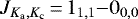 ) transition at 607.349 GHz (Matsushima et al. 2001). Detected thus far only towards the solar type protostar IRAS16293-2422 (Butner et al. 2007; Vastel et al. 2010), it is unlikely that there is significant contamination from D2 O absorption in our spectra. Observations of the o-H2O+ spectra which were performed in double sideband mode, covered the 13CO (10−9) transition at 1101.3 GHz (Zink et al. 1990) in the LSB, alongside the o-H2O+ line in the USB. This 13CO emission feature blends with the LOS absorption profile of o-H2O+ towards AG10.472+00.027 and to a lesser extent with that of AG19.609−00.234 and AG31.412+00.307.
While, it is imperative to accurately model the degree of contamination in order to determine physical quantities within the velocity intervals concerned, there are several uncertainties in the “residual” absorption obtained from fitting the observed emission features. Therefore, we do not model contributions from the different contaminants present along the different sight lines but rather exclude the corresponding velocity intervals from our modelled fits and analysis. However, by doing so, it is possible that we ignore impeding emission features and emission line-wings, which remain undetected because they are absorbed away below the continuum. This can lead to potential uncertainties in the derived optical depths particularly in the velocity intervals neighbouring the emission. In the following sections, we carry out a qualitative and quantitative comparison between the (uncontaminated) absorption features, for the different species and for each individual source.
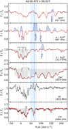 |
Fig. 2 From top to bottom: Normalised spectra showing transitions of ArH+, p-H2O+, o-H2O+, OH+, HI, and CH, towards AG10.472+00.027, in black. The vertical dashed blue line and blue shaded regions mark the systemic velocity and the typical velocity dispersion of the source. The vertical dashed grey lines indicate the main absorption dips. Red curves display the Wiener filter fit to the observed spectra except for the HI spectra. The relative intensities of the hyperfine structure (hfs) components of the o-H2O+ and the OH+ and CH transitions are shown in black above their respective spectra and the grey shaded regions display their hfs deconvolvedspectra. Contaminating emission features are marked by the blue hatched lines and are excluded from the modelled fit and analysis. |
 |
Fig. 3 Same as Fig. 2 but towards AG19.609−00.234. There is no OH+ and CH spectra of the transitions studied here, available for this source. |
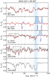 |
Fig. 4 Same as Fig. 2 but towards AG31.412+00.307. There is no CH spectrum of the transitions studied here, available for this source. |
3.1 Line-of-sight properties
The Galactic sources we have selected in this work, which predominantly provide the background radiation for our absorption studies, are luminous (L > 104 L⊙) as they are dusty envelopes around young stellar objects with typical signposts of massive star-formation such as class II methanol masers and/or ultracompact (UC) HII regions. Much of this work addresses the investigation of trends of various quantities with Galactocentric distance. To allow this, the spectrum towards each sight line is divided into local standard of rest (LSR) velocity intervals that correspond to absorption features arising from different spiral-arm and inter-arm crossings. The velocities of these LOS absorption components are then mapped on a model of Galactic rotation to relate them to the Galactocentric distance, RGAL. The values for RGAL were computed by assuming a flat rotation curve, with the distance between the Sun and the Galactic centre (GC), R0, and the Sun’s orbital velocity, Θ0, assumed to be 8.15 kpc and 247 km s−1, respectively,as determined by Reid et al. (2019). We have also compared our distance solutions with those reported in Urquhart et al. (2018), who have analysed the kinematic properties of dense clumps present in the ATLASGAL survey, which covers our sources. Furthermore, it is to be noted that our assumption of a flat rotation curve is only valid for RGAL ≳ 4 kpc as shown in Fig. 11 of Reid et al. (2019). For smaller values of RGAL and for a general check on all distances, we employed the parallax-based distance calculator accessible from the website of the Bar and Spiral Structure Legacy survey (BeSSeL)6.
In general, over velocity intervals that correspond to the envelopes of the individual molecular cloud cores, the “systemic” velocities, ArH+ shows very weak to almost no absorption unlike the other molecules. The absence of ArH+ at these velocities is in line with chemical models that predict ArH+ to exist exclusively in low-density atomic gas,  –10−2 (Schilke et al. 2014; Neufeld & Wolfire 2016). As discussed in Sect. 2, the LSB of the SEPIA660 receiver was tuned to cover the p-H2O+ transitions near 604 and 607 GHz. Invariably across our entire sample of sources, we do not detect any clear absorption features from the p-H2O+ line at 604 GHz at an average noise level of 23 mK (at a spectral resolution of 1.1 km s−1), owing to its weaker line strength in comparison to the p-H2O+ line at 607 GHz. Hence, we do not discuss the former p-H2O+ transition in the remainder of our study.
AG10.472+00.027
The sight line towards AG10.472+ 0.027, which is at a distance of 8.55 kpc (Sanna et al. 2014), crosses several spiral arms in the inner Galaxy. This results in a broad absorption spectrum covering an LSR velocity range from −35 to 180 km s−1. All the molecules show absorption at υLSR between − 35 and 48 km s−1, which arises partly from inter-arm gas and partly from the near-side crossing of the Sagittarius arm and Scutum-Centaurus arm. Within this velocity range, the absorption profiles form a nearly continuous blend except for p-H2O+, which has an unidentified emission feature at ~ 3 km s−1 and generally narrower features. In contrast, the OH+ absorption covers a larger velocity range than the other molecules and almost saturates within 0 and 45 km s−1. The features at υLSR > 80 km s−1 are associated with the 3 kpc arm and the Galactic bar. Both p-H2O+ and o-H2O+ only weakly absorb at υLSR > 130 km s−1; the former is also affected by some unknown emission features. However, ArH+ shows absorption features similar to OH+ with strong absorption dips at 80 and 127 km s−1. The high-velocity component likely traces gas that lies beyond the GC belonging to the 135 km s−1 arm (Sormani & Magorrian 2015). CH has a narrow absorption dip at ~ 150 km s−1 unlike the other atomic gas tracers, while ArH+ and OH+ have prominent absorption at 170 km s−1. The corresponding HI spectrum with very little continuum, has a poor signal-to-noise ratio, which results in negative values in regions withlarge noise levels. However, the Bayesian analysis of the HI spectrum described in Winkel et al. (2017), which is used to derive the column density and spin temperature, correctly accounts for these noise effects amongst other spatial variations along the LOS.
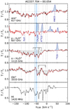 |
Fig. 7 Same as Fig. 2 but towards AG337.704−00.054. There is no CH spectrum of the transitions studied here, available for this source. |
AG19.609-00.234
It is a massive star-forming clump at a heliocentric distance of 12.7 kpc (Urquhart et al. 2014) with an absorption spectrum extending from − 10 to 150 km s−1. The absorption at υLSR between − 10 and 20 km s−1 primarily traces inter-arm gas between the Perseus and outer arms and parts of the Aquila Rift, followed by weak absorption near 27 km s−1 from the envelope of the molecular cloud. While the absorption dips between 35 and 74 km s−1 (seen most clearly in the o-H2O+ spectrum), arising from the near and far side crossings of the Sagittarius spiral-arm. Unsurprisingly, there is no ArH+ absorption at 40 km s−1 but ArH+ shows red-shifted absorption tracing layers of infalling material associated with the molecular cloud. Infalling signatures towards this hot molecular cloud have previously been studied by Furuya et al. (2011), whose observations of the J = 3 → 2 transitions of 13CO and 18CO show inverse P-Cygni profiles or red-shifted absorption alongside a blue-shifted emission component. The ArH+ spectrum also shows a narrow absorption feature at 80 km s−1 possibly from the edge of the spiral arm. The strongest absorption feature seen in the ArH+ spectrum lies close to 113 km s−1 from the Scutum-Centaurius arm, which is notably a weaker component in the o-H2O+ and HI spectra.
AG31.412+00.307
Located on the Scutum-Centaurus arm at a distance of 5.55 kpc (Moisés et al. 2011), the line of sight towards this young-stellar object, AG31.412+00.307, crosses the Sagittarius arm at velocities roughly between 30 and 55 km s−1 and the Perseus arm at velocities <20 km s−1. The ArH+ absorption profile mimics that of HI with only minor offsets in the peak velocities (< 1 km s−1) of the absorption components. Moreover, the ArH+ absorption seen close to the source’s intrinsic velocity at 98 km s−1 traces infalling material. Unfortunately, because of the poor signal-to-noise ratio of the OH+ spectrum it is very difficult to make an accurate component-wise comparison.
AG330.954-00.182
Located at a distance of 5.3 kpc (Wienen et al. 2015), AG330.954−00.182 lies in the Norma spiral arm and is a bright ATLASGAL 870 μm source in the fourth quadrant. It has an absorption profile that extends from − 130 to 20 km s−1. The gas between − 60 and 20 km s−1 traces the near and far-side crossings of both the Scutum-Centaurius as well as the Sagittarius spiral-arms. The ArH+ spectrum shows absorption at − 115 km s−1, a feature which is not present in the other species. There is weak ArH+ absorption close to 90 km s−1, which maybe associated with the molecular cloud itself. The line profile resembles a single absorption component as seen in the HI spectrum and not two components of comparable depths as seen in the OH+ and o-H2O+ spectra.
AG332.826-00.549
The sight line towards AG332.826− 00.549, which has a near kinematic distance of 3.6 kpc (Moisés et al. 2011), primarily traces the Scutum-Centaurius and Sagittarius spiral-arms. Overall, the observed profiles of the different species in terms of their shape, are in concordance with each other. Akin to the ArH+ spectrum, the spectra of the other ionised species in our study, p-, and o-H2O+, and OH+, all show their strongest absorption features near − 40 km s−1 and red-shifted absorption tracing infalling material similar to G19.609−00.234. This feature whilst present in the HI spectrum is much weaker in comparison to the absorption at velocities corresponding to the molecular cloud which is expected, but is weaker, also in comparison to other LOS features and is not prominent in the CH spectrum.
AG337.704-00.054
At a distance of ~12.3 kpc (Green & McClure-Griffiths 2011), AG337.704−00.054 is one of the most distant Galactic sources in our sample. Absorption features cover a range of velocities from − 135 to ~ +20 km s−1. The LOS absorption at negative velocities between –140 and –60 km s−1 arise from the 3 kpc and the Norma spiral arms. The ArH+ spectrum shows contiguous absorption over the entire velocity range cited, unlike the spectra of the other molecular ions and even HI.
AG351.581-00.352
It is a bright and compact HII region at a distance of 6.8 kpc (Green & McClure-Griffiths 2011) that is located between the 3 kpc arm and the beginning of the Norma arm. Notably, ArH+ has its strongest absorption peak at − 27 km s−1, arising from the Scutum arm while OH+ and o-H2O+ both peak close to 50 km s−1, tracing gas from the Norma arm. At the current rms noise level of the ArH+ spectrum, itis difficult to ascertain the presence of absorption components at positive velocities that are clearly observed in the spectra of the other molecular ions, HI and CH.
3.2 Spectral fitting
The optical depth, τ is determined from the radiative transfer equation for the specific case of absorption spectroscopy (Tl = Tce−τ), given knowledge of the continuum background temperature, Tc. The optical depth profile is then analysed using the Wiener filter fitting technique as described in Jacob et al. (2019). This two-step fitting procedure first fits the spectrum based on the Wiener filter, which minimises the mean square error between the model and observations and then deconvolves the hfs from the observed spectrum, if any. When fitting lines that do not exhibit hfs, the procedure simply assumes that there is only a single hfs component whose frequency corresponds to that of the fine-structure transition itself. In addition to the observed spectrum and the spectroscopic parameters of the line to be fit, the only other input parameter required by the Wiener filter technique is the spectral noise, which is assumed to be independent of the signal. Furthermore, the technique also assumes that the lines are optically thin and under conditions of local thermodynamic equilibrium (LTE).
3.3 Column density
From the resultant optical depth profile, we determine the column densities per velocity interval, dN/dυ, using
![Mathematical equation: \begin{equation*} \left(\frac{\text{d}N}{\text{d}\upsilon}\right)_{i}\,{=}\,\frac{8\pi\nu^3_{i} }{c^3 } \frac{Q(T_{\text{ex}})}{g_{\text{u}} A_{\text{E}}} \text{e}^{E_{\text{u}}/T_{\text{ex}}} \left[ \text{exp} \left(\frac{h\nu_{i}}{k_{\text{B}}T_{\text{ex}}}\right) - 1 \right]^{-1} (\tau_{i})\end{equation*}](/articles/aa/full_html/2020/11/aa39197-20/aa39197-20-eq9.png) (1)
(1)
for each velocity channel, i. For a given hfs transition, all of the above spectroscopic terms remain constant, except for the partition function, Q, which itself is a function of the rotation temperature, Trot. Under conditions of LTE Trot is equal to the excitation temperature, Tex. We further assume that almost all the molecules occupy the ground rotational state where the excitation temperature, Tex, is determined by the cosmic microwave background radiation, TCMB, of 2.73 K. This is a valid assumption for the conditions that prevail in diffuse regions where the gas densities, (n(H) ≤ 100 cm−3), are sufficiently low enough that collisional excitation becomes unimportant. However, this assumption may no longer be valid for those features that arise from the dense envelopes of the molecular clouds in which collisions can dominate, resulting in higher excitation temperatures. Therefore, the column densities derived by integrating Eq. (1) over velocity intervals associated with the molecular cloud components, only represent lower limits to the column density values. Combining all our sources, we are broadly ableto identify a total of 38 distinct absorption features; however, we could only assign 33, 15, and 35 of these features to ArH+, p-, and o-H2O+ absorption, respectively, due to the blending of different species present along the different LOS. The column densities that we have derived for each species and towards each sight line are summarised in Table 3. The ArH+ column densities are found to vary between ~6 × 10¹¹ and 1013 cm−2 across inter-arm and spiral-arm clouds along the different sight lines. The derived p-H2O+ column density values also show a similar variation, towards our sample of sources.
The accuracy of the reported column density values is mainly limited by uncertainties present in the continuum level and not the absolute temperature calibration. The errors in the WF analysis are computed using Bayesian methods to sample a posterior distribution of the optical depths. In this approach, we sampled 5000 artificial spectra each generated by iteratively adding a pseudo-random noise contribution to the absorption spectra, of each of the different species prior to applying the WF deconvolution. The standard deviation in the additive noise is fixed to be the same as that of the line free part of the spectrum. The deconvolved optical depths and the subsequently derived column densities per velocity interval, sample a point in the channel-wise distribution of the column densities, across all the spectra. Since, the posterior of the optical depths is not normally distributed, we describe the profiles of the distributions by using the median and the inter-quartile range. This removes any bias introduced on the mean by the asymmetric nature of the distributions. We then determined the sample mean and standard deviation following Ivezić et al. (2019). The deviations from the newly derived mean are then used to determine the errors.
Synopsis of derived quantities.
3.4 Cosmic-ray ionisation rate
Ionisation by cosmic-rays is the primary ionisation mechanism that drives ion-molecular reactions within diffuse atomic clouds. As discussed in Sect. 1, the formation of ArH+ is initiated by the ionisation of argon atoms by cosmic-rays. Therefore, knowledge of the primary ionisation rate per hydrogen atom, ζp (H), is vital for ourunderstanding of the ensuing chemistry. In this section, we investigate the cosmic-ray ionisation rates towards our sample of sources, which can be determined by analysing the steady-state ion-molecular chemistry of OH+ and o-H2O+.
In the diffuse ISM, both OH+ and o-H2O+ are mainly destroyed either via reactions with H2 or recombination with an e−. The relevant reactions are summarised below, alongside their reaction rates which are taken from Tran et al. (2018), Mitchell (1990), and the KIDA database7 (Wakelam et al. 2012):
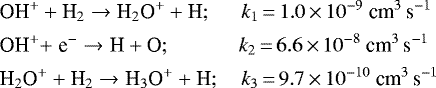
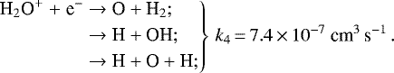
Since our analysis does not require the exact branching information between the products formed from the recombination of H2O+ with an e−, k4 cites the total reaction rate. The rates for reactions with H2 are independentof the gas temperature, T, while, the recombination reactions have a weak dependence on it with k ∝ T−0.49. The reaction rates for the latter were computed at a temperature of 100 K corresponding to the typical HI spin temperature along the LOS towards the sources in our sample. Moreover, the transitions that we study mainly probe warm diffuse gas with typical values of T between 30 and 100 K (Snow & McCall 2006). Decreasing the temperature from 100 K to 30 K would result in an 80% increase in the reaction rates.
Following the steady-state analysis presented in Indriolo et al. (2012), the cosmic-ray ionisation rate may be written as
![Mathematical equation: \begin{equation*} \epsilon \zeta_{\text{p}}(\text{H})\,{=}\,\frac{N(\text{OH}^+)}{N(\text{H})}n_{\text{H}}\left[ \frac{f_{\text{H}_{2}}}{2}k_{1} + x_{\text{e}}k_{2} \right] \,,\end{equation*}](/articles/aa/full_html/2020/11/aa39197-20/aa39197-20-eq12.png) (2)
(2)
where k1 and k2 are the rates of the reactions between OH+ and H2, and OH+ and a free electron. As introduced in Neufeld et al. (2010), ɛ is an efficiency factor that represents the efficiency with which ionised H forms OH+. The efficiency parameter was predicted by chemical models (Hollenbach et al. 2012) to vary between 5% and 20% as it is dependent on the physical properties of the cloud. Observationally, this efficiency has been determined only towards the W51 region by Indriolo et al. (2012) to be 7 ± 4%, using the spectroscopy of OH+, H2O+ and H . For our calculations we use a value of ɛ = 7%.
While, N(OH+) and N(H) are determined from observations, nH refers to the gas density, for which we adopt a value of nH ≈ 35 cm−3. This value corresponds to the mean density of the cold neutral medium at the solar circle, RGAL ≈ 8.3 kpc (Indriolo et al. 2012, 2015). The electronabundance, xe in diffuse clouds is often considered to be equal to the fractional abundance of ionised carbon, xe = 1.5 × 10⁻⁴ (Sofia et al. 2004). Under the conditions that prevail over the diffuse regions of the ISM, this is a valid assumption because C+ is responsible for most of the free electrons and therefore the electron abundance, with negligible contributions from other ionised species. This assumption however, breaks down in regions of high ζp (H)∕n(H) where ionisation by H becomes significant, like in the Galactic centre (Le Petit et al. 2016).
The molecular fraction,  is typically defined as
 (3)
(3)
and can be re-written in terms of the N(OH+)∕N(H2O+) ratio by
 (4)
(4)
where, N(H2O+) is the total column density of H2O+, N(H2O+) = N(p-H2O+) + N(o-H2O+). For those velocity intervals for which absorption is detected only in one of either the o- or p-H2O+ lines we present a lower limit on the molecular fraction. The molecular hydrogen fractions hence derived using Eq. (4) has a median value of  . Alternatively, we can also compute the column-averaged molecular hydrogen fraction
  by using N(CH) as a tracer for N(H2), following the relationship between the two molecules estimated by Sheffer et al. (2008), [CH]/[H2] =
  . However, the column-averaged molecular fractions derived towards the different velocity intervals using CH column densities are higher (by almost an order of magnitude) than those derived using Eq. (4). This difference arises from the fact that CH resides in, and therefore traces molecular gas unlike both OH+ and H2O+.
The cosmic-ray ionisation rates we infer from the steady-state chemistry of OH+ (and H2O+) using Eq. (2) lie between 1.8 × 10⁻¹⁷ and 1.3 × 10⁻¹⁵ s−1. Resulting in an average value of ζp (H) = (2.28 ± 0.34) × 10−16 s−1 towards the sight lines studied here. The uncertainties in ζp (H) quoted in this work reflect the uncertainties in the derived column density values. The impact of the uncertainties associated with the assumptions made in this analysis, on the derived cosmic-ray ionisation rates are discussed in more detail in Schilke et al. (2014) and Indriolo et al. (2015). Within the statistical errors, this result is consistent with the cosmic-ray ionisation rates that were previously determined using H by Indriolo & McCall (2012) and OH+ and H2O+ by Indriolo et al. (2015); Neufeld & Wolfire (2017).
The derived values for the cosmic-ray ionisation rate are summarised in Table 3 and in Fig. 9 we display their variation with galactocentric distance. The cosmic-ray ionisation rates in the extreme environment of the GC, are generally found to be higher than in the general Galactic environment and cover a range of values over two orders of magnitude between ~ 10−16 and 1.83 × 10⁻¹⁴ s−1 as discussed in Indriolo et al. (2015) and references therein. At galactocentric distances <5 kpc the ionisation rates that we derive in this study are comparable to those derived by Indriolo et al. (2015) at larger distances. This might hint to the fact that the gradient seen by these authors at 3 < RGAL < 5 kpc from the LOS components towards the GC sources (like M-0.13-0.08, M-0.02-0.07, Sgr B2(M) and Sgr B2(N)) are higher than the average cosmic-ray ionisation rate present in these spiral arms because these velocity components may contain contributions from the GC. At RGAL > 5 kpc, the cosmic-ray ionisation rates derived in this work are systematically lower than those derived in Indriolo et al. (2015) however, several of the ionisation rates derived by these authors, that lie below ~ 5 × 10⁻¹⁷ s−1 only represent upper limits to the cosmic-ray ionisation rates.
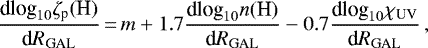
We derive a slope, m, of − 0.012 from ζp (H) versus RGAL, for galactocentric distances that lie within 4 < RGAL < 8.5 kpc. Our analysis thus far assumes a constant value for n(H) equal to themean gas density of cold gas near the solar circle, which itself varies with galactocentric distances as discussed in Wolfire et al. (2003). Neufeld & Wolfire (2017) took this, as well as variations in the UV radiation field (χUV) over Galactic scales into account and described the galactocentric gradient in the cosmic-ray ionisation rate as follows,
 (5)
(5)
where, ![Mathematical equation: $\zeta_{\text{p}}(\text{H})/n(\text{H}) \propto \left[ \chi_{\text{UV}}/n(\text{H})\right]^{-0.7}$](/articles/aa/full_html/2020/11/aa39197-20/aa39197-20-eq22.png) . From the models presented in Wolfire et al. (2003), which characterise the nature of neutral gas present within the Galactic disk, d log10n(H)∕dRGAL and d log10χUV∕dRGAL have values of − 0.110 kpc−1 and − 0.106 kpc−1, respectively. Using, the scale length, [dlnζp(H)∕ d RGAL]−1, hence derived and the mean value of the cosmic-ray ionisation rate of their data-set, these authors derive the Galactic gradient to be
. From the models presented in Wolfire et al. (2003), which characterise the nature of neutral gas present within the Galactic disk, d log10n(H)∕dRGAL and d log10χUV∕dRGAL have values of − 0.110 kpc−1 and − 0.106 kpc−1, respectively. Using, the scale length, [dlnζp(H)∕ d RGAL]−1, hence derived and the mean value of the cosmic-ray ionisation rate of their data-set, these authors derive the Galactic gradient to be  RGAL]∕ 4.7 kpc) × 10−16 s−1, where Ro = 8.5 kpc and RGAL between 3–8.5 kpc. Following the analysis presented by Neufeld & Wolfire (2017), briefly discussed above, we derive a revised cosmic-ray ionisation rate gradient as, ζp(H) = (1.80 ±
 ![Mathematical equation: $0.70)\,\text{exp}\left[ \left(R_{\text{o}} - R_{\text{GAL}}\right)/{3.46~\text{kpc}}\right]\,{\times}\,10^{-16}\,\text{s}^{-1}$](/articles/aa/full_html/2020/11/aa39197-20/aa39197-20-eq24.png) using a scale length of 3.46 kpc and a mean cosmic-ray ionisation rate of (1.80 ± 0.70) × 10−16 s−1 (where the value in parenthesis is the standard error), across the combined sample of sight lines studied in Indriolo et al. (2015) and this work for galactocentric distances that lie within 4 < RGAL < 8.5 kpc and a gas density of 35 cm−3. We have excluded the ζp(H) values derived for the Galactic centre sources.
using a scale length of 3.46 kpc and a mean cosmic-ray ionisation rate of (1.80 ± 0.70) × 10−16 s−1 (where the value in parenthesis is the standard error), across the combined sample of sight lines studied in Indriolo et al. (2015) and this work for galactocentric distances that lie within 4 < RGAL < 8.5 kpc and a gas density of 35 cm−3. We have excluded the ζp(H) values derived for the Galactic centre sources.
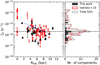 |
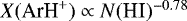
Fig. 9 Left: Cosmic-ray ionisation rates derived from OH+ vs. galactocentric distance. The filled black triangles and unfilled red diamonds represent ζp (H) values derived from the LOS absorption features observed in this study and in Indriolo et al. (2015), respectively. The dashed black line marks the median value of the total ζp (H) distributions. The solid-dotted line represents the derived cosmic-ray ionisation rate gradient. Right: Histogram distributionsof ζp(H) derived in this work displayed in black, that from Indriolo et al. (2012) in red, and the combined distribution by the hatched grey region. |
3.5 H2O+ analysis
For H2O+, the lower energy spin variant is o-H2O+ owing to its C2v symmetry and 2 B1 ground state, unlike the case of H2O, for which the lowest energy level is the 000 level of the p-H2O spin isomer. The lowest ortho- and para-rotational levels of H2O+ have an energy difference of ≈30.1 K and the fine structure levels of the ortho ground state (I = 1) further undergo hfs splitting, while those of the para (I = 0) state do not. Under the typical conditions present in the diffuse ISM, the rotational temperature (as discussed in Sect. 3.3) is close to TCMB, which makes it valid to assume that most of the molecules will exist in the lowest ortho and para rotational states.
The conversion between the ortho- and para-states of a species, typically occurs via proton exchange reactions with either atomic H or H2. Since, atomic H is the most abundant species along our diffuse LOS, we expect the proton exchange in H2O+ to primarily take place via gas phase reactions with H. Moreover, in the presence of H2, H2O+ ions may energetically react to form H3 O+ and a hydrogen atom:

Since, the two spin states can be moderately coupled via collisions, the OPR is given by
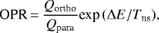 (6)
(6)
where Qortho and Qpara represent the partition functions of the respective states, ΔE is the energy difference between the two states, ΔE = −30.1 K (it is negative because the lowest ortho state lies at a lower energy level than the lowest para state, unlike in H2O) and Tns is the nuclear spin temperature. At low temperatures, the partition function of the para- and ortho-states are governed by the degeneracy of their lowest fine-structure and hfs levels, respectively. Both states have the same quantum numbers and degeneracy, which implies that, as the rotational temperature approaches 0 K, the ratio of the partition functions approaches unity (see, Appendix A of Schilke et al. 2010). Therefore, in the analysis that follows we assume that, Qortho = Qpara. Since, the largest uncertainty in our derived OPR arises from the uncertainties in the absorption features of the p-H2O+ profile, we only carry out this analysis in those velocity intervals that are the least contaminated. From our column density calculations, we derive OPR values between ~1 : 1 and 4.5:1, which is compatible with the equilibrium value of three, within the error bars. We find a mean OPR for H2O+ of 2.1:1 which corresponds to a mean nuclear spin temperature of 41 K.
4 Discussion
4.1 Properties of ArH+ as a tracer of atomic gas
We derive ArH+ abundances relative to atomic H column densities, X(ArH+) = N(ArH+)∕N(Hi), that span over roughly two orders of magnitude varying between 4.6 × 10⁻¹¹ and 1.6 × 10⁻⁸, with an average value of (1.6 ± 1.3) × 10−9. In Fig. 10, by combining our ArH+ data points with values from the sight lines studied in Schilke et al. (2014), we compare the derived column densities and abundances of ArH+ with atomic hydrogen column densities. Over the entire range, the ArH+ column densities cluster at N(H) = (2.7 ± 1.6) × 1021 cm−2. We observe a large spread in the ArH+ abundances derived, even for the molecular cloud (MC) components. This is mainly because of the high optical depths of the HI data and to a lesser extent because, towards some of the sources in our sample, we see that ArH+ traces layers of infalling material associated with the molecular cloud. Figure 10 does not reveal a strong correlation between ArH+ and HI, as we had expected because HI traces different phases of the ISM with varying degrees of molecular fraction. Moreover, the HI emission at certain velocity intervals may be a superposition of both the near- and far-side components of the Milky Way, often leading to blending effects which can potentially bias the inferred spin temperatures and column densities.
We subjected the entire ArH+/HI data-set to a regression analysis and find log(X(ArH+)) = (−0.80 ± 0.20) log(N(H)) + (7.84 ± 4.28) with a correlation coefficient of 38% at a 99.99% confidence level. This translates to a power-law relation between ArH+ and HI column densities of 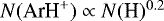 . This can be viewed as a global relation as the behaviour of the power-law index (or slope in logarithmic-scales) does not appreciably vary between the diffuse LOS and dense molecular cloud components and there is no clear power-law break. Observations in the past have shown that considerable amounts of HI gas exist within molecular clouds, whose population is maintained via the destruction of H2 by cosmic-rays (e.g. Wannier et al. 1991; Kuchar & Bania 1993). Hence, the HI gas along any given LOS in our study, also contains gas that resides inside molecular clouds with a fractional abundance, [H]/[H2], ~ 0.1%. From Fig. 10, we find that as N(HI) increases, X(ArH+) decreases due to the increasing amounts of dense gas traced by HI gas. It is therefore clear that only a small fraction of the HI gas traces the same cloud population as that traced by ArH+. Based on the astrochemical models presented by Schilke et al. (2014), if we assume the abundance of ArH+ to be a constant (X(ArH+) = 2 × 10⁻¹⁰) for cloud depths ≤ 0.01 mag which corresponds to an average molecular fraction of 10−3, then we findthat only 17.3% of the LOS HI gas traces these conditions.
As detailed in Schilke et al. (2014), ArH+ is destroyed primarily via proton transfer reactions with H2 or atomic oxygen, and photodissociation:
![Mathematical equation: \begin{align*} \text{ArH}^{+} &+ \text{H}_{2} \rightarrow \text{Ar} + \text{H}_{3}^{+} \, ; \quad \quad \quad k_{5}\,{=}\,8\,{\times}\, 10^{-10}~\text{cm}^{3}~\text{s}^{-1} \\[2pt] \text{ArH}^{+} &+ \text{O} \rightarrow \text{Ar} + \text{OH}^{+} \, ; \quad \quad \, \, k_{6}\,{=}\,8\,{\times}\, 10^{-10}~\text{cm}^{3}~\text{s}^{-1} \\[2pt] \text{ArH}^{+} &+ \text{h}\nu \rightarrow \text{Ar}^+ + \text{H} \, ; \, \quad \quad \ \ k_{7}\,{=}\,1.0\,{\times}\, 10^{-11}\chi_{\text{UV}}f_{\text{A}}~\text{s}^{-1} \,. \end{align*}](/articles/aa/full_html/2020/11/aa39197-20/aa39197-20-eq28.png)
The photodissociation rate of ArH+ was estimated by Alekseyev et al. (2007) to be ~1.0 × 10⁻¹¹fA s−1 for an unshielded cloud model uniformly surrounded by the standard Draine UV interstellar radiation field. However, for the particular environment of the Crab nebula, the photodissociation rate has been calculated to be much higher at 1.9 × 10⁻⁹ s−1 (Roueff et al. 2014). The attenuation factor, fA, is given by an exponential integral and is a function of visual extinction, Av. Schilke et al. (2014) derive values of fA between 0.30 and 0.56, increasing as you move outwards from the centre of the cloud, for a cloud model with Av = 0.3. In our analysis, we use a value of 0.43 for fA, mid-way through the computed range of values. We further assume a gas density n(H) = 35 cm−3, an atomic oxygen abundance (relative to H nuclei) of 3.9 × 10⁻⁴ and an argon abundance close to its solar abundance of 3.2 × 10⁻⁶ (Lodders 2008). Using these values the cosmic-ray ionisation rate is approximated as follows,

Re-arranging Eq. (8), we express it in terms of  , as follows:
![Mathematical equation: \begin{equation*} f_{\text{H}_{2}}\,{=}\,2.68\,{\times}\,10^{3} \left[ \frac{\zeta_{\text{p}}(\text{H})}{X(\text{ArH}^{+})} - 4.17\,{\times}\,10^{-7} \right] \,\end{equation*}](/articles/aa/full_html/2020/11/aa39197-20/aa39197-20-eq31.png) (9)
(9)
Substituting the ArH+ abundances derived from observations into Eq. (9) and by assuming that the ArH+ ions are exposed to the same cosmic-ray flux as OH+ and H2O+, we derive the molecular fraction of the gas probed by ArH+. Of course, there is the caveat that ArH+ does not necessarily trace the same gas as that traced by both OH+, and H2O+ and therefore, need not be exposed to the same cosmic-ray ionisation flux. Our results find ArH+ to probe a range of molecular fractions, with a median value of 8.8 × 10⁻⁴. This is in agreement with the results obtained from chemical models presented in Neufeld & Wolfire (2017), which suggest that the observed ArH+ abundance resides in regions with molecular fractions that are at most 10−2. The molecular fraction analysis displayed in Fig. 11, derived from the observed abundances of ArH+, OH+, and CH using Eqs. (9), (4), and (3), respectively, clearly shows the transition between different phases of the ISM, from the diffuse atomic to the diffuse/translucent molecular gas.
We further compare the Galactic radial distribution of the azimuthally averaged ArH+, OH+ and o-H2O+ column densities with those of HI towards a combined sample set that contains sight lines presented in both Schilke et al. (2014) and this work. The probability distributions of the different column densities were computed using the kernel density estimation method, for a Gaussian kernel. This analysis was carried out for galactocentric distances between 4 and 9 kpc, since we have only a limited number of data points at RGAL < 4 kpc and RGAL > 9 kpc making it difficult to comment on the nature of the distribution at these distances. Although we only cover a small number of background continuum sources in the Galaxy (but sample many LOS), the distribution of N(Hi) versus galactocentric radii presented in Fig. 12, for the common RGAL coverage, resembles that of the Hi emissivity presented by Pineda et al. (2013) for 500 LOS across the Galaxy. The Hi column densities we derived peak at RGAL = 5.1 kpc corresponding to the intersection of the Perseus and Norma spiral-arms with a possible narrower peak between 7.5 and 8 kpc arising fromthe Scutum-Crux arm.
Atomic gas predominantly exists in thermal equilibrium between two phases of the ISM namely, the cold neutral medium (CNM) and the warm neutral medium (WNM). Pineda et al. (2013) used the HI emission line to trace the total gas column but were able to separate the relative contributions from gas in the CNM, and WNM by using constraints from HI absorption studies. Their analysis revealed that the CNM is the dominant component within the inner Galaxy peaking close to the 5 kpc arm while it is the WNM that contributes towards the peak in the outer Galaxy at 8 kpc. The radial distribution of the ArH+ column densities peaks between 4 and 4.5 kpc slightly offset from the HI peak with almost an anti-correlation at 4.7 kpc. At RGAL > 5 kpc, the N(ArH+) profile decreases mimicking the radial trend followed by the CNM component. However, there maybe a potential increase in the column densities near 8 kpc but we cannot as yet confirm the presence of this peak as we require more sight line information towards the outer Galaxy (RGAL > 8 kpc). If ArH+ does have a WNM component our results are in agreement with the idea that ArH+ is formed in the outermost layers of the cloud. The column density distributions of OH+ and o-H2O+ on the other hand, peak behind the 5 kpc ring, with a significant contribution at 4–4.5 kpc similar to the ArH+, which we do not see in the HI data. Since, the column densities at 7 and 7.5 kpc are much greater than that at 8 kpc for OH+ and o-H2O+ distributions, the presence of a secondary peak in the outer Galaxy, seems unlikely.
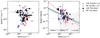 |
Fig. 10 Left: N(ArH+) vs. N(H). Right: X(ArH+) = N(ArH+)∕N(Hi) vs. N(H). The data points include column density values derived towards the MC and LOS features from our sample of sources indicated by filled grey and black triangles, as well as those from Schilke et al. (2014) marked by unfilled red and blue diamonds, respectively. The solid black line displays the power-law relation to the combined data-set,
|
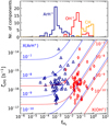 |
Fig. 11 Top: Distribution of molecular gas fraction ( |


Summary of correlation power-law fit parameters as a function of N(ArH+) (NX).
4.2 Comparison of ArH+ with other atomic gas tracers
In this section, we investigate the correlation between the column density of ArH+ with that of other tracers of atomic gas such as OH+ and o-H2O+ and with molecular gas traced by CH. Combining our sample with data taken by Schilke et al. (2014); Indriolo et al. (2015); Wiesemeyer et al. (2016, 2018) and Jacob et al. (2019), in Fig. 13 we show the correlation between the 62, 57, and 40 sight lines towards which both ArH+ and o-H2O+ (left), OH+ (centre), and CH (right), respectively, have been detected. The distribution of the OH+ and o-H2O+ column density components associated with the molecular cloud environment of these SFRs displays a large dispersion in comparison to the LOS components with no clear correlations over the range of ArH+ column densities probed, reflected by weakly negative correlation coefficients of − 0.02 and − 0.08, respectively. In addition, as expected the ArH+ and CH column densities derived over molecular cloud velocities are anti-correlated with a correlation coefficient of −0.30. This emphasises that ArH+ probes cloud layers with slightly different properties from those traced by not only CH but also o-H2O+ and OH+.
The global correlation of the LOS components are described using a power-law of the form  , where c is the scaling factor and p is the power-law index, and NX, NY represent the column densities of the different species. The fit parameters and correlation coefficients (at a 99.99% confidence interval), corresponding to the derived correlations, amongst the different species across all the data points (both LOS and MC) are summarised in Table 4. We chose to describe the correlation using a power-law trend after comparing the residuals and correlation coefficients obtained from this fit with those obtained from fitting a linear regression of the form, NY = mNX + c. Moreover, a positive y-axis intercept would suggest the presence of either o-H2O+, OH+ or H2 in the absence of ArH+ or vice versa for a negative intercept and interpreting this would require the aid of additional chemical models.
As discussed earlier, the different species may not be spatially co-existent and the observed correlations may result from the fact that an increase in the total column density of each sight line subsequently, increases the column density of each phase. Therefore, one would expect there to be a weak correlation between the column densities in each phase, along any given LOS. We investigate this by comparing the abundances of these species as a function of the molecular fraction of the gas they trace. From Fig. 14 it is clear that ArH+ and OH+ and H2O+ all trace the same cloud layers only in a small range of molecular gas fractions between 1.5 × 10⁻³–3 × 10⁻², while CH traces the denser molecular gas. We further notice that the distribution of CH abundances shows a positive correlation with  while, that of OH+ is anti-correlated and both, ArH+, and H2O+ remain almost constant at X(ArH+) = (4.7 ± 0.2) × 10−10 and X(H2O+) = (1.3 ± 1.0) × 10−9.
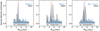 |
Fig. 12 Kernel density distributions of the of ArH+ (left), OH+ (centre), and o-H2O+ (right) column densities as a function of galactocentric distances (black hatched regions). The sampling of the distribution is displayed as a rug plot and is indicated by the solid black lines below the density curves. The dashed red line marks the 5 kpc ring. |
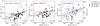 |
Fig. 13 Comparison of the ArH+ column density to that of o-H2O+ (left), OH+ (centre), and CH (right). Black and grey filled triangles indicate the column density values derived within velocity intervals corresponding to LOS absorption and molecular cloud (MC) towards the Galactic sources presented in this study. Additionally, the blue and red unfilled diamonds mark the LOS and MC column densities derived towards the sources discussed in Schilke et al. (2014). The solid black curve represents the best fit to the combined data set including both the LOS and MC components with the grey shaded region displaying the 1 σ interval of the weighted regression. The dashed cyan and dashed-dotted pink curves represent the fits to only the LOS and only the MC components, respectively. |
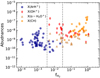 |
Fig. 14 Molecular abundances with respect to atomic hydrogen as a function of molecular gas fraction ( |

4.3 H2O+ ortho-to-para ratio
Of the 14 absorption components for which we were able to compute the OPR of H2O+, 9 show values significantly lower than the value of 3:1 with 6 of the derived OPRs lying close to unity. Such low values of the OPR are conceivable as the corresponding spin temperatures (derived in the absence of a rotational excitation term as in Eq. (6)) reflect the typical kinetic temperatures of the diffuse clouds. However, amongst some sight line components the OPR is as high as  which point to cold environments with spin temperatures as low as 20 K. Perhaps similar to studies of the OPR of H2 by Flower et al. (2006), the OPR of H2O+ at these low temperatures maybe governed by the kinematic rates of its formation and destruction processes.
Moreover, the OPR of H2 greatly impacts the observed OPR of H2O+ because the latter is synthesised in diffuse clouds via an exothermic reaction between OH+ and H2. To assess this, requires the determination of the fraction of ortho- and para-H2O+ formed from the reacting fractions of both ortho- and para-H2 states whilst abiding by the spin selection rules. After estimating the fractions of ortho- and para-H2O+, Herbst (2015) derived an OPR for H2O+ of 2:1 and concludes that this approach fails as it requires all the reacting, parent H2 molecules to exist in the ortho-state in order to reproduce the higher observed OPR values.
In Fig. 15, we investigate the impact of cosmic-ray ionisation rates on the OPR ratio of H2O+. In the discussion that follows we do not include those data points corresponding to GC sources studied in Indriolo et al. (2015), as the unique nature of this region results in very high cosmic-ray ionisation rates (ζp(H) > 10−15 s−1). As can be seen, the OPR of H2O+ thermalises to a value of three when increasing ζp(H) from ~2.8 × 10⁻¹⁷ up to ~ 4.5 × 10⁻¹⁶ s−1. This is because an increase in the cosmic-ray flux results in an increase in the abundance of atomic H, thus efficiently driving the (H2O+ + H) proton-exchange reaction. Within the cited error bars the OPR saturates to a value of three at a median ζp (H) = (1.8 ± 0.2) × 10−16 s−1. The lack of a correlation beyond this value may suggest that the destruction of H2O+ via reactions with H2 and free electrons dominates over the proton exchange reaction. If this is true, then the increase in the OPR is controlled by the kinematics of the destruction pathways. Such variations in the destruction reactions of both the ortho and the para forms have been experimentally detected for the dissociative recombination reaction of the H ion by Glosík et al. (2010). Such a preferential recombination of the para-state of H2O+ over that of its ortho-state might explain the higher observed values of the OPR. However, laboratory measurements of the recombination cross-sections of rotational excitation of the ortho- and para-states of H2O+ are required to confirm whether the lowest para state undergoes recombination reactions faster than its ortho counterpart. Alternatively, in regions with high values of ζp (H) where protons are largely abundant, reactions between H2O and protons can be a competing formation pathway for the production of H2O+ ions (k ~ 1−4 × 10⁻⁸ cm3 s−1 for T = 10–100 K). This further complicates the analysis as we now have to take into account the OPR of the reacting H2O molecules and its corresponding efficiency in producing either ortho- or para-H2O+ states. However, this requires detailed modelling of the dust-grain and gas-phase processes that govern the OPR of H2O, which is beyond the scope of this paper. The main source of uncertainty in this analysis is in the column density estimates of p-H2O+, which may be under-estimated in velocity intervals that are affected by contamination from emission lines or over-estimated in regions with D2O absorption.
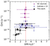 |
Fig. 15 Observed OPR of H2O+ vs. the cosmic-ray ionisation rates derived using the steady state analysis of the OH+ and H2O+. The results from this work are marked by black triangles while those from Indriolo et al. (2015) are displayed by blue diamonds. For comparison we display the OPR of H2O+ derived by these authors towards GC sight lines using purple stars. The dashed red line marks the equilibrium OPR value of three. |
5 Conclusions
In this paper we present our observations searching for ArH+ absorption along the LOS towards seven SFRs in the Galaxy. Our successful search towards all our targets has doubled the sample of known ArH+ detections, which allows us to constrain the physical properties of the absorbing medium. We determined ArH+ column densities over 33 distinct velocity intervals corresponding to spiral-arm and inter-arm crossings and find a mean ArH+ abundance, X(ArH+) = N(ArH+)∕N(H) of 1.5 ± 0.9 × 10⁻⁹ with a power-law relationship between ArH+ and atomic hydrogen of  . We do not detect any ArH+ absorption at the systemic velocities of these sources except for signatures that trace infalling material.
By analysing the steady state chemistry of OH+, and o-H2O+ along with the abundances determined from observations, we derived molecular hydrogen fractions,  , of the order of 10−2, consistent with previous determinations of
  by Neufeld & Wolfire (2016). We subsequently derived cosmic-ray ionisation rates with a mean ζp (H) value of (2.28 ± 0.34) × 10−16 s−1. Assuming that the observed population of ArH+ ions are alsoexposed to the same amount of cosmic-ray irradiation, we derived the molecular fraction of gas traced by ArH+ to be on average 8.8 × 10⁻⁴. Moreover, the distribution of the column densities of ArH+–OH+, ArH+–o-H2O+ and ArH+–CH, while being moderately correlated for material along the LOS, shows almost no correlation or even a negative one for the material associated with the molecular cloud environments. These results observationally highlight that ArH+ traces a different cloud population than its diffuse atomic gas counterparts OH+, and o-H2O+ and the diffuse molecular gas tracer CH. Additionally, the Galactic distribution profile of the ArH+ column densities resembles that of HI within the inner Galaxy (RGAL ≲ 7 kpc). A pronounced peak at 5 kpc is dominated by contributions from the CNM component of atomic gas (Pineda et al. 2013), while the WNM component primarily contributes in the outer Galaxy. While we find a larger dispersion of N(ArH+) values at RGAL > 7 kpc, our analysis does not clearly find evidence for a secondary peak at 8 kpc as it is limited by the number of sight lines. Proving or disproving the presence of this feature, to ultimately distinguish between the different components of the neutral gas probed by the ArH+, would require further observations covering sight lines present in the outer Galaxy. While our results confirm the value of ArH+ as a tracer of purely atomic gas, there are several sources of uncertainties that can bias them. These include the validity of the assumptions we made in computing the molecular fraction and the systematic effects that the blending of the HI emission particularly at and close to the sources’ systemic velocities has on the derived column densities.
Through our H2O+ analysis, we have derived OPRs that are both above and below the expected equilibrium value of three with a mean value of 2.10 ± 1.0. This corresponds to a nuclear spin temperature of 41 K which is within the typical range of gas temperatures observed for diffuse clouds. However, a majority of the velocity components show OPRs close to unity, increasing steeply to the standard value of three with increasing cosmic-ray ionisation rates up to ζp (H) = (1.8 ± 0.2) × 10−16 s−1. Beyond this value, the OPR shows no correlation with ζp(H), indicating that from that point on reactions with H2 take over as the dominant destruction pathway in its chemistry. The general deviations of the OPR of H2O+ may also be inherited from the OPR of its parent species, namely H2 or H2O and the efficiency in converting between the two spin states.
Acknowledgements
This publication is based on data acquired with the Atacama Pathfinder Experiment (APEX) under the project id M-0103.F-9519C-2019. APEX is a collaboration between the Max-Planck-Institut fur Radioastronomie, the European Southern Observatory, and the Onsala Space Observatory. We would like to express our gratitude to the APEX staff and science team for their continued assistance in carrying out the observations presented in this work. The authors would like to thank the anonymous referee for their careful review of the article and valuable input and Marijke Haverkorn for providing us with the SGPS continuum data for AG10.472+00.027. We are thankful to the developers of the C++ and Python libraries and for making them available as open-source software. In particular, this research has made use of the NumPy (van der Walt et al. 2011), SciPy (Jones et al. 2001) and matplotlib (Hunter 2007) packages.
Appendix A H I analysis
In this appendix we present the Hi absorption (Ton) and emission spectra (Toff), along with derived quantities such as the optical depth, spin temperature and column density. The solid black curve in the continuum normalised on-source spectrum, Ton,obs∕Tsou,obscont (top panel) represents the absorption profile smoothed to the resolution of the emission data. Classically the off-source spectrum is taken from a position next to the source of interested (well outside of the beam width). However, in the Milky Way disk, HI is subject to strong spatial fluctuations and using a single off position would be error prone. Therefore, in Winkel et al. (2017) a spatial filtering technique using a ring (or doughnut-shaped) kernel was applied to obtain an interpolated brightness temperature, shown in the second panel (black curve). For comparison, in the panel displaying spin temperatures, we also plot the brightness temperaturein blue and lastly, the column density panel also displays the uncorrected column density profile,  . The blue and grey shaded regions indicate the 1σ (68% percentile) and 3σ (99.7% percentile) confidence intervals, respectively. Additionally in each panel, we mark the systemic velocity and velocity dispersion of each source by the dashed pink line and shaded pink regions, respectively. A detailed description is presented in Winkel et al. (2017).
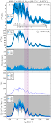 |
Fig. A.1 From top to bottom: HI absorption and emission spectra, optical depth, spin temperature, and HI column density towards AG10.472+00.027. The pink dashed line and shaded region mark the systemic velocity of the source and highlight the velocity dispersion of the source. |
Appendix B Continuum level uncertainties
In this Appendix we briefly discuss the reliability of the absolute calibration of the continuum brightness temperatures used in our analysis. As a first check, we binned our observations across scans (time), towards each individual source over velocity intervals/channels previously used to estimate the continuum and baseline. Assessing the relative fluctuations in the continuum level will reveal the stability of its measurement. From Fig. B.1, it can be seen that the scatter in the continuum level, over different scans, is less than 10% for all the sources in our study except AG330.954−00.182 and AG332.826−00.549 which shows a slightly large scatter of 18%. Not showing any major variations, leads us to conclude that the continuum levels are fairly reliable. It is important to note here that the observations were carried out using the wobbling secondary with a fast switching rate which was essential in removing any drifts due to atmospheric instabilities.
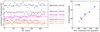 |
Fig. B.1 Left: Continuum fluctuations across scans. The dashed lines represent the median continuum level for each source. Right: Correlation between the observed ArH+ continuum flux and the 870 μm continuum flux. |
As discussed earlier in the text, we have also carried out a comparison between the continuum flux levels of our ArH+ observations with the peak fluxes obtained from the 870 μm continuum data from the ATLASGAL survey. We see that our data is well correlated with the 870 μm continuum emission with a relative scatter <5%.
Appendix C Column density profiles
In this Appendix we present the column density profiles for all the species studied in this work except HI (which is already presented inAppendix A) towards the entire source sample in this study.
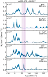 |
Fig. C.1 Topto bottom: Column density per velocity channel of ArH+, p-H2O+, o-H2O+, OH+, and CH towards G10.472+00.027. The blue shaded region represents the uncertainties while the pink dashed line, and shaded region mark the systemic velocity of the source and highlight the velocity dispersion of the source. The dashed blue lines indicate those velocity intervals that were omitted from the fitting routine due to contamination. |
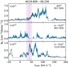 |
Fig. C.2 Same as Fig. C.1 but towards G19.609−00.234. There is no OH+ and CH spectra of the transitions studied here, available for this source. |
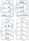 |
Fig. C.3 Same as Fig. C.1 but towards (clockwise from top-left) G31.412+00.307, G337.704−00.054, G332.826−00.549, and G330.954−00.182. There is no CH spectrum of the transitions studied here, available for G31.412+00.307 and G337.704−00.054. |
References
- Alekseyev, A. B., Liebermann, H.-P., & Buenker, R. J. 2007, Phys. Chem. Chem. Phys. (Incorp. Faraday Trans.), 9, 5088 [CrossRef] [Google Scholar]
- Barlow, M. J., Swinyard, B. M., Owen, P. J., et al. 2013, Science, 342, 1343 [NASA ADS] [CrossRef] [PubMed] [Google Scholar]
- Bartlett, N., & Lohmann, D. 1962, J. Chem. Soc. (Resumed), 5253 [CrossRef] [Google Scholar]
- Belitsky, V., Lapkin, I., Fredrixon, M., et al. 2018, A&A, 612, A23 [NASA ADS] [CrossRef] [EDP Sciences] [Google Scholar]
- Belloche, A., Müller, H. S. P., Menten, K. M., Schilke, P., & Comito, C. 2013, A&A, 559, A47 [NASA ADS] [CrossRef] [EDP Sciences] [Google Scholar]
- Belov, S. P., Winnewisser, G., & Herbst, E. 1995, J. Mol. Spectr., 174, 253 [NASA ADS] [CrossRef] [Google Scholar]
- Bergin, E. A., Phillips, T. G., Comito, C., et al. 2010, A&A, 521, A20 [Google Scholar]
- Beuther, H., Bihr, S., Rugel, M., et al. 2016, A&A, 595, A32 [NASA ADS] [CrossRef] [EDP Sciences] [Google Scholar]
- Bialy, S., Neufeld, D., Wolfire, M., Sternberg, A., & Burkhart, B. 2019, ApJ, 885, 109 [CrossRef] [Google Scholar]
- Bizzocchi, L., Dore, L., Degli Esposti, C., & Tamassia, F. 2016, ApJ, 820, L26 [NASA ADS] [CrossRef] [Google Scholar]
- Black, J. H. 1978, ApJ, 222, 125 [NASA ADS] [CrossRef] [Google Scholar]
- Butner, H. M., Charnley, S. B., Ceccarelli, C., et al. 2007, ApJ, 659, L137 [NASA ADS] [CrossRef] [Google Scholar]
- Coxon, J. A., & Hajigeorgiou, P. G. 2016, J. Mol. Spectr., 330, 63 [CrossRef] [Google Scholar]
- Csengeri, T., Urquhart, J. S., Schuller, F., et al. 2014, A&A, 565, A75 [NASA ADS] [CrossRef] [EDP Sciences] [Google Scholar]
- de Graauw, T., Helmich, F. P., Phillips, T. G., et al. 2010, A&A, 518, L6 [NASA ADS] [CrossRef] [EDP Sciences] [Google Scholar]
- Flower, D. R., Pineau Des Forêts, G., & Walmsley, C. M. 2006, A&A, 449, 621 [NASA ADS] [CrossRef] [EDP Sciences] [Google Scholar]
- Furuya, R. S., Cesaroni, R., & Shinnaga, H. 2011, A&A, 525, A72 [NASA ADS] [CrossRef] [EDP Sciences] [Google Scholar]
- Galli, D., & Palla, F. 2013, ARA&A, 51, 163 [NASA ADS] [CrossRef] [Google Scholar]
- Gerin, M., de Luca, M., Black, J., et al. 2010, A&A, 518, L110 [NASA ADS] [CrossRef] [EDP Sciences] [Google Scholar]
- Glosík, J., Plašil, R., Kotrík, T., et al. 2010, Mol. Phys., 108, 2253 [CrossRef] [Google Scholar]
- Green, J. A., & McClure-Griffiths, N. M. 2011, MNRAS, 417, 2500 [NASA ADS] [CrossRef] [Google Scholar]
- Griffin, M. J., Abergel, A., Abreu, A., et al. 2010, A&A, 518, A3 [NASA ADS] [CrossRef] [EDP Sciences] [Google Scholar]
- Güsten, R., Wiesemeyer, H., Neufeld, D., et al. 2019, Nature, 568, 357 [CrossRef] [Google Scholar]
- Herbst, E. 2015, in EUR. Phys. J. Web Conf., 84, 06002 [CrossRef] [Google Scholar]
- Hesper, R., Khudchenko, A., Lindemulder, M., et al. 2018, in Proceedings of 29th International Symposium on Space Terahertz Technology [Google Scholar]
- Hocking, W. H., Gerry, M. C. L., & Winnewisser, G. 1975, Can. J. Phys., 53, 1869 [NASA ADS] [CrossRef] [Google Scholar]
- Hogness, T. R., & Lunn, E. G. 1925, Phys. Rev., 26, 44 [NASA ADS] [CrossRef] [Google Scholar]
- Hollenbach, D., Kaufman, M. J., Neufeld, D., Wolfire, M., & Goicoechea, J. R. 2012, ApJ, 754, 105 [NASA ADS] [CrossRef] [Google Scholar]
- Hunter, J. D. 2007, Comput. Sci. Eng., 9, 90 [NASA ADS] [CrossRef] [Google Scholar]
- Indriolo, N., & McCall, B. J. 2012, ApJ, 745, 91 [NASA ADS] [CrossRef] [Google Scholar]
- Indriolo, N., Neufeld, D. A., Gerin, M., et al. 2012, ApJ, 758, 83 [NASA ADS] [CrossRef] [Google Scholar]
- Indriolo, N., Neufeld, D. A., Gerin, M., et al. 2015, ApJ, 800, 40 [NASA ADS] [CrossRef] [Google Scholar]
- Ivezić, Ž., Connelly, A. J., Vand erplas, J. T., & Gray, A. 2019, Statistics, Data Mining, and Machine Learning in Astronomy (Princeton University Press) [CrossRef] [Google Scholar]
- Jacob, A. M., Menten, K. M., Wiesemeyer, H., et al. 2019, A&A, 632, A60 [CrossRef] [EDP Sciences] [Google Scholar]
- Johnson, D. R., Lovas, F. J., & Kirchhoff, W. H. 1972, J. Phys. Chem. Ref. Data, 1, 1011 [NASA ADS] [CrossRef] [Google Scholar]
- Jones, E., Oliphant, T., Peterson, P., et al. 2001, SciPy: Open Source Scientific Tools for Python [Google Scholar]
- Kuchar, T. A., & Bania, T. M. 1993, ApJ, 414, 664 [NASA ADS] [CrossRef] [Google Scholar]
- Lattanzi, V., Walters, A., Drouin, B. J., & Pearson, J. C. 2007, ApJ, 662, 771 [NASA ADS] [CrossRef] [Google Scholar]
- Le Petit, F., Ruaud, M., Bron, E., et al. 2016, A&A, 585, A105 [NASA ADS] [CrossRef] [EDP Sciences] [Google Scholar]
- Lodders, K. 2008, ApJ, 674, 607 [CrossRef] [Google Scholar]
- Matsushima, F., Matsunaga, M., Qian, G.-Y., et al. 2001, J. Mol. Spectr., 206, 41 [CrossRef] [Google Scholar]
- McClure-Griffiths, N. M., Dickey, J. M., Gaensler, B. M., et al. 2005, ApJS, 158, 178 [NASA ADS] [CrossRef] [Google Scholar]
- Mitchell, J. B. A. 1990, Phys. Rep., 186, 215 [NASA ADS] [CrossRef] [Google Scholar]
- Moisés, A. P., Damineli, A., Figuerêdo, E., et al. 2011, MNRAS, 411, 705 [NASA ADS] [CrossRef] [Google Scholar]
- Müller, H. S. P., Muller, S., Schilke, P., et al. 2015, A&A, 582, L4 [NASA ADS] [CrossRef] [EDP Sciences] [Google Scholar]
- Müller, H. S. P., Schlöder, F., Stutzki, J., & Winnewisser, G. 2005, J. Mol. Struct., 742, 215 [NASA ADS] [CrossRef] [Google Scholar]
- Muller, S., Müller, H. S. P., Black, J. H., et al. 2016, A&A, 595, A128 [NASA ADS] [CrossRef] [EDP Sciences] [Google Scholar]
- Neufeld, D. A., Goicoechea, J. R., Sonnentrucker, P., et al. 2010, A&A, 521, L10 [NASA ADS] [CrossRef] [EDP Sciences] [Google Scholar]
- Neufeld, D. A., & Wolfire, M. G. 2016, ApJ, 826, 183 [NASA ADS] [CrossRef] [Google Scholar]
- Neufeld, D. A., & Wolfire, M. G. 2017, ApJ, 845, 163 [Google Scholar]
- Otarola, A., De Breuck, C., Travouillon, T., et al. 2019, PASP, 131, 045001 [NASA ADS] [CrossRef] [Google Scholar]
- Pardo, J. R., Cernicharo, J., & Serabyn, E. 2001, IEEE Trans. Antennas Propag., 49, 1683 [Google Scholar]
- Pineda, J. L., Langer, W. D., Velusamy, T., & Goldsmith, P. F. 2013, A&A, 554, A103 [NASA ADS] [CrossRef] [EDP Sciences] [Google Scholar]
- Priestley, F. D., Barlow, M. J., & Viti, S. 2017, MNRAS, 472, 4444 [NASA ADS] [CrossRef] [Google Scholar]
- Reid, M. J., Menten, K. M., Brunthaler, A., et al. 2019, ApJ, 885, 131 [NASA ADS] [CrossRef] [Google Scholar]
- Roach, A., & Kuntz, P. 1970, J. Chem. Soc. D: Chem. Commun., 1336 [CrossRef] [Google Scholar]
- Roueff, E., Alekseyev, A. B., & Le Bourlot, J. 2014, A&A, 566, A30 [NASA ADS] [CrossRef] [EDP Sciences] [Google Scholar]
- Sanna, A., Reid, M. J., Menten, K. M., et al. 2014, ApJ, 781, 108 [NASA ADS] [CrossRef] [Google Scholar]
- Schilke, P., Comito, C., Müller, H. S. P., et al. 2010, A&A, 521, A11 [NASA ADS] [CrossRef] [EDP Sciences] [Google Scholar]
- Schilke, P., Neufeld, D. A., Müller, H. S. P., et al. 2014, A&A, 566, A29 [NASA ADS] [CrossRef] [EDP Sciences] [Google Scholar]
- Schuller, F., Menten, K. M., Contreras, Y., et al. 2009, A&A, 504, 415 [NASA ADS] [CrossRef] [EDP Sciences] [Google Scholar]
- Sheffer, Y., Rogers, M., Federman, S. R., et al. 2008, ApJ, 687, 1075 [NASA ADS] [CrossRef] [Google Scholar]
- Snow, T. P., & McCall, B. J. 2006, ARA&A, 44, 367 [NASA ADS] [CrossRef] [Google Scholar]
- Sofia, U. J., Lauroesch, J. T., Meyer, D. M., & Cartledge, S. I. B. 2004, ApJ, 605, 272 [NASA ADS] [CrossRef] [Google Scholar]
- Sormani, M. C., & Magorrian, J. 2015, MNRAS, 446, 4186 [NASA ADS] [CrossRef] [Google Scholar]
- Swinyard, B. M., Ade, P., Baluteau, J. P., et al. 2010, A&A, 518, A4 [NASA ADS] [CrossRef] [EDP Sciences] [Google Scholar]
- Theis, R. A., Morgan, W. J., & Fortenberry, R. C. 2015, MNRAS, 446, 195 [CrossRef] [Google Scholar]
- Tran, T. D., Rednyk, S., Kovalenko, A., et al. 2018, ApJ, 854, 25 [NASA ADS] [CrossRef] [Google Scholar]
- Urquhart, J. S., Figura, C. C., Moore, T. J. T., et al. 2014, MNRAS, 437, 1791 [NASA ADS] [CrossRef] [Google Scholar]
- Urquhart, J. S., König, C., Giannetti, A., et al. 2018, MNRAS, 473, 1059 [NASA ADS] [CrossRef] [Google Scholar]
- van der Walt, S., Colbert, S. C., & Varoquaux, G. 2011, Comput. Sci. Eng., 13, 22 [Google Scholar]
- van Dishoeck, E. F., Kristensen, L. E., Benz, A. O., et al. 2011, PASP, 123, 138 [NASA ADS] [CrossRef] [Google Scholar]
- Vastel, C., Ceccarelli, C., Caux, E., et al. 2010, A&A, 521, L31 [NASA ADS] [CrossRef] [EDP Sciences] [Google Scholar]
- Wakelam, V., Herbst, E., Loison, J. C., et al. 2012, ApJS, 199, 21 [NASA ADS] [CrossRef] [Google Scholar]
- Wannier, P. G., Andersson, B. G., Morris, M., & Lichten, S. M. 1991, ApJS, 75, 987 [CrossRef] [Google Scholar]
- Wienen, M., Wyrowski, F., Menten, K. M., et al. 2015, A&A, 579, A91 [NASA ADS] [CrossRef] [EDP Sciences] [Google Scholar]
- Wiesemeyer, H., Güsten, R., Heyminck, S., et al. 2016, A&A, 585, A76 [NASA ADS] [CrossRef] [EDP Sciences] [Google Scholar]
- Wiesemeyer, H., Güsten, R., Menten, K. M., et al. 2018, A&A, 612, A37 [NASA ADS] [CrossRef] [EDP Sciences] [Google Scholar]
- Winkel, B., Wiesemeyer, H., Menten, K. M., et al. 2017, A&A, 600, A2 [CrossRef] [EDP Sciences] [Google Scholar]
- Wolfire, M. G., McKee, C. F., Hollenbach, D., & Tielens, A. G. G. M. 2003, ApJ, 587, 278 [NASA ADS] [CrossRef] [Google Scholar]
- Wootten, A., & Thompson, A. R. 2009, IEEE Proc., 97, 1463 [NASA ADS] [CrossRef] [Google Scholar]
- Zink, L. R., De Natale, P., Pavone, F. S., et al. 1990, J. Mol. Spectr., 143, 304 [NASA ADS] [CrossRef] [Google Scholar]
Meaning that the PWV content was 1.08 mm or lower for half of the covered time period.
Software package developed by IRAM, see https://www.iram.fr/IRAMFR/GILDAS/ for more information regarding GILDAS packages.
THOR is The HI/OH/Recombination line survey of the inner Milky Way observed using the Very Large Array (VLA) in C-configuration (Beuther et al. 2016).
SGPS is the Southern Galactic Plane Survey, which combines data from the Australia Telescope Compact Array and the Parkes Radio Telescope.
All Tables
All Figures
|
Fig. 1 Calculated atmospheric zenith transmission of the entire 450 μm submillimeter window for the site of the APEX telescope for three values of the precipitable water vapour column: 0.25 mm (dark blue), 0.40 mm (orange), and 1.08 mm (red). The grey shaded regions mark the 8 GHz frequency windows covered by each of the two sidebands (separated by 8 GHz) of the SEPIA660 receiver. The dashed brown and pink lines mark frequencies of the p-H2O+ and ArH+ lines discussed in this work, respectively. |
| In the text | |
|
Fig. 2 From top to bottom: Normalised spectra showing transitions of ArH+, p-H2O+, o-H2O+, OH+, HI, and CH, towards AG10.472+00.027, in black. The vertical dashed blue line and blue shaded regions mark the systemic velocity and the typical velocity dispersion of the source. The vertical dashed grey lines indicate the main absorption dips. Red curves display the Wiener filter fit to the observed spectra except for the HI spectra. The relative intensities of the hyperfine structure (hfs) components of the o-H2O+ and the OH+ and CH transitions are shown in black above their respective spectra and the grey shaded regions display their hfs deconvolvedspectra. Contaminating emission features are marked by the blue hatched lines and are excluded from the modelled fit and analysis. |
| In the text | |
|
Fig. 3 Same as Fig. 2 but towards AG19.609−00.234. There is no OH+ and CH spectra of the transitions studied here, available for this source. |
| In the text | |
|
Fig. 4 Same as Fig. 2 but towards AG31.412+00.307. There is no CH spectrum of the transitions studied here, available for this source. |
| In the text | |
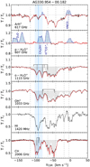 |
Fig. 5 Same as Fig. 2 but towards AG330.954−00.182. |
| In the text | |
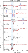 |
Fig. 6 Same as Fig. 2 but towards AG332.826−00.549. |
| In the text | |
|
Fig. 7 Same as Fig. 2 but towards AG337.704−00.054. There is no CH spectrum of the transitions studied here, available for this source. |
| In the text | |
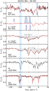 |
Fig. 8 Same as Fig. 2 but towards AG351.581−00.352. |
| In the text | |
|
Fig. 9 Left: Cosmic-ray ionisation rates derived from OH+ vs. galactocentric distance. The filled black triangles and unfilled red diamonds represent ζp (H) values derived from the LOS absorption features observed in this study and in Indriolo et al. (2015), respectively. The dashed black line marks the median value of the total ζp (H) distributions. The solid-dotted line represents the derived cosmic-ray ionisation rate gradient. Right: Histogram distributionsof ζp(H) derived in this work displayed in black, that from Indriolo et al. (2012) in red, and the combined distribution by the hatched grey region. |
| In the text | |
|
Fig. 10 Left: N(ArH+) vs. N(H). Right: X(ArH+) = N(ArH+)∕N(Hi) vs. N(H). The data points include column density values derived towards the MC and LOS features from our sample of sources indicated by filled grey and black triangles, as well as those from Schilke et al. (2014) marked by unfilled red and blue diamonds, respectively. The solid black line displays the power-law relation to the combined data-set,
|
| In the text | |
|
Fig. 11 Top: Distribution of molecular gas fraction ( |
| In the text | |
|
Fig. 12 Kernel density distributions of the of ArH+ (left), OH+ (centre), and o-H2O+ (right) column densities as a function of galactocentric distances (black hatched regions). The sampling of the distribution is displayed as a rug plot and is indicated by the solid black lines below the density curves. The dashed red line marks the 5 kpc ring. |
| In the text | |
|
Fig. 13 Comparison of the ArH+ column density to that of o-H2O+ (left), OH+ (centre), and CH (right). Black and grey filled triangles indicate the column density values derived within velocity intervals corresponding to LOS absorption and molecular cloud (MC) towards the Galactic sources presented in this study. Additionally, the blue and red unfilled diamonds mark the LOS and MC column densities derived towards the sources discussed in Schilke et al. (2014). The solid black curve represents the best fit to the combined data set including both the LOS and MC components with the grey shaded region displaying the 1 σ interval of the weighted regression. The dashed cyan and dashed-dotted pink curves represent the fits to only the LOS and only the MC components, respectively. |
| In the text | |
|
Fig. 14 Molecular abundances with respect to atomic hydrogen as a function of molecular gas fraction ( |
| In the text | |
|
Fig. 15 Observed OPR of H2O+ vs. the cosmic-ray ionisation rates derived using the steady state analysis of the OH+ and H2O+. The results from this work are marked by black triangles while those from Indriolo et al. (2015) are displayed by blue diamonds. For comparison we display the OPR of H2O+ derived by these authors towards GC sight lines using purple stars. The dashed red line marks the equilibrium OPR value of three. |
| In the text | |
|
Fig. A.1 From top to bottom: HI absorption and emission spectra, optical depth, spin temperature, and HI column density towards AG10.472+00.027. The pink dashed line and shaded region mark the systemic velocity of the source and highlight the velocity dispersion of the source. |
| In the text | |
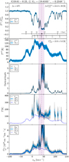 |
Fig. A.2 Same as Fig. A.1 but towards AG19.609−00.234. |
| In the text | |
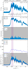 |
Fig. A.3 Same as Fig. A.1 but towards AG330.954−00.182. |
| In the text | |
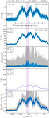 |
Fig. A.4 Same as Fig. A.1 but towards AG332.826−00.549. |
| In the text | |
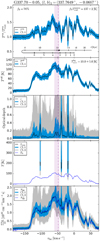 |
Fig. A.5 Same as Fig. A.1 but towards AG337.704−00.054. |
| In the text | |
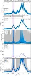 |
Fig. A.6 Same as Fig. A.1 but towards AG351.581−00.352. |
| In the text | |
|
Fig. B.1 Left: Continuum fluctuations across scans. The dashed lines represent the median continuum level for each source. Right: Correlation between the observed ArH+ continuum flux and the 870 μm continuum flux. |
| In the text | |
|
Fig. C.1 Topto bottom: Column density per velocity channel of ArH+, p-H2O+, o-H2O+, OH+, and CH towards G10.472+00.027. The blue shaded region represents the uncertainties while the pink dashed line, and shaded region mark the systemic velocity of the source and highlight the velocity dispersion of the source. The dashed blue lines indicate those velocity intervals that were omitted from the fitting routine due to contamination. |
| In the text | |
|
Fig. C.2 Same as Fig. C.1 but towards G19.609−00.234. There is no OH+ and CH spectra of the transitions studied here, available for this source. |
| In the text | |
|
Fig. C.3 Same as Fig. C.1 but towards (clockwise from top-left) G31.412+00.307, G337.704−00.054, G332.826−00.549, and G330.954−00.182. There is no CH spectrum of the transitions studied here, available for G31.412+00.307 and G337.704−00.054. |
| In the text | |
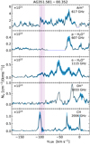 |
Fig. C.4 Same as Fig. C.1 but towards G351.581+00.352. |
| In the text | |
Current usage metrics show cumulative count of Article Views (full-text article views including HTML views, PDF and ePub downloads, according to the available data) and Abstracts Views on Vision4Press platform.
Data correspond to usage on the plateform after 2015. The current usage metrics is available 48-96 hours after online publication and is updated daily on week days.
Initial download of the metrics may take a while.