| Issue |
A&A
Volume 640, August 2020
|
|
|---|---|---|
| Article Number | A107 | |
| Number of page(s) | 41 | |
| Section | Extragalactic astronomy | |
| DOI | https://doi.org/10.1051/0004-6361/201935855 | |
| Published online | 21 August 2020 | |
The VANDELS survey: Discovery of massive overdensities of galaxies at z > 2
Location of Lyα-emitting galaxies with respect to environment⋆
1
Instituto de Astrofísica, Universidad Católica de Chile, Vicuña Mackenna 4860, Santiago, Chile
e-mail: This email address is being protected from spambots. You need JavaScript enabled to view it.
2
ESO-Chile, Alonso de Cordova 3107, Vitacura, Chile
3
Núcleo de Astronomía, Facultad de Ingeniería, Universidad Diego Portales, Av. Ejército 441, Santiago, Chile
4
INAF-Osservatorio Astronomico di Roma, Via Frascati 33, 00078 Monteporzio, Roma, Italy
5
INAF-Osservatorio di Astrofisica e Scienza dello Spazio di Bologna, via Gobetti 93/3, 40129 Bologna, Italy
6
INAF-Osservatorio Astronomico di Trieste, via G.B. Tiepolo 11, 34143 Trieste, Italy
7
Departamento de Astronomía, Universidad de La Serena, Av. Juan Cisternas 1200 Norte, La Serena, Chile
8
INAF-Istituto di Astrofisica Spaziale e Fisica Cosmica Milano, via Bassini 15, 20133 Milano, Italy
9
Sorbonne Universités, UPMC-CNRS, UMR7095, Institut d’Astrophysique de Paris, 75014 Paris, France
10
Space Telescope Science Institute, 3700 San Martin Drive, Baltimore, MD 21218, USA
11
Dipartimento di Fisica e Astronomia, Universitá di Bologna, Via Gobetti 93/2, 40129 Bologna, Italy
12
Centro de Astroingeniería, Facultad de Física, Pontificia Universidad Católica de Chile, Casilla 306, Santiago 22, Chile
13
Millennium Institute of Astrophysics (MAS), Nuncio Monseñor Sótero Sanz 100, Providencia, Saniago, Chile
14
Space Science Institute, 4750 Walnut Street, Suite 205, Boulder, Colorado 80301, USA
15
Instituto de Investigación Multidisciplinar en Ciencia y Tecnología, Universidad de La Serena, Raúl Bitrán 1305, La Serena, Chile
16
Institute for Astronomy, University of Edinburgh, Royal Observatory, Edinburgh EH9 3HJ, UK
17
Tianjin Normal Univeristy, Binshuixilu 393, 300387 Tianjin, PR China
Received:
9
May
2019
Accepted:
11
June
2020
Abstract
Context. The advent of deep, multi-wavelength surveys, together with the availability of extensive numerical simulations, now allow us for the systematic search and study of (proto)clusters and their surrounding environment as a function of redshift.
Aims. We aim to define the environment and to identify overdensities in the VANDELS Chandra Deep Field-South (CDFS) and UKIDSS Ultra Deep Survey (UDS) fields. We want to investigate whether we can use Lyα emission to obtain additional information of the environment properties and whether Lyα emitters show different characteristics as a function of their environment.
Methods. We estimated local densities using a three-dimensional algorithm which works in the RA-dec-redshift space. We took advantage of the physical parameters of all the sources in the VANDELS fields to study their properties as a function of environment. In particular, we focused on the rest-frame U − V color to evaluate the stage of evolution of the galaxies located in the overdensities and in the field. Then we selected a sample of 131 Lyα-emitting galaxies (EW(Lyα) > 0 Å), unbiased with respect to environmental density, from the first two seasons of the VANDELS survey to study their location with respect to the over- or under-dense environment and infer whether they are useful tracers of overdense regions.
Results. We identify 13 (proto)cluster candidates in the CDFS and nine in the UDS at 2 < z < 4, based on photometric and spectroscopic redshifts from VANDELS and from all the available literature. No significant difference is observed in the rest-frame U − V color between field and galaxies located within the identified overdensities, but the star-forming galaxies in overdense regions tend to be more massive and to have low specific SFRs than in the field. We study the distribution of the VANDELS Lyα emitters (LAEVs) and we find that Lyα emitters lie preferentially outside of overdense regions as the majority of the galaxies with spectroscopic redshifts from VANDELS. The LAEVs in overdense regions tend to have low Lyα equivalent widths and low specific SFRs, and they also tend to be more massive than the LAEVs in the field. Their stacked Lyα profile shows a dominant red peak and a hint of a blue peak. There is evidence that their Lyα emission is more extended and offset with respect to the UV continuum.
Conclusions. LAEVs are likely to be influenced by the environment. In fact, our results favour a scenario that implies outflows of low expansion velocities and high HI column densities for galaxies in overdense regions. An outflow with low expansion velocity could be related to the way galaxies are forming stars in overdense regions; the high HI column density can be a consequence of the gravitational potential of the overdensity. Therefore, Lyα-emitting galaxies can provide useful insights on the environment in which they reside.
Key words: galaxies: high-redshift / galaxies: kinematics and dynamics / galaxies: interactions / galaxies: clusters: general
Based on data obtained with the European Southern Observatory Very Large Telescope, Paranal, Chile, under Large Program ID 194.A-2003.
© ESO 2020
1. Introduction
Clusters of galaxies are interesting laboratories for the study of the evolution of galaxies as a function of their environment and they are important cosmological tracers to constrain models of the Universe. The maximum mass which can collapse and virialize at any epoch depends on ΩM, the power spectrum σ8, and the dark energy equation of state. Hence, the study of a statistically significant sample of clusters, whose mass can be reliably measured, is a powerful tool for deriving observational constraints on cosmological models.
A mature cluster can be recognized for the presence of a red sequence (significant number of galaxies with similar colors redder than the field galaxies, for example Gladders et al. 2000). However, the formation and the evolution of clusters of galaxies with a developed red sequence is still under investigation. Relatively recent results at low redshift (z≤ 0.5) have revealed that the influence of the potential well of the cluster extends much farther than previously thought, up to three times the effective radius (a size that contains about 40% of the total mass of the cluster), implying a larger environmental influence on the galaxies and groups in the vicinity of the cluster (see, e.g., Haines et al. 2015). Groups interacting with clusters have clearly shown the importance of lower mass structures in stripping the gas from galaxies before they fall into the larger potential well of the cluster, the so-called pre-processing (Cortese et al. 2006).
Going back in time, evolved galaxy overdensities have been observed up to redshift z ∼ 2 (Kodama et al. 2007; Willis et al. 2013; Andreon et al. 2014). These structures (more commonly referred to as protoclusters1, Overzier 2016) assembled at z ∼ 4 (e.g., Miller et al. 2018; Lemaux et al. 2018). However, there are also observations of dense structures at z ∼ 2 in which the galaxies are more massive and older than the field galaxies, but do not show a red sequence (e.g., Steidel et al. 2005).
Different methods have been used to identify protoclusters at z > 2, including the detection of overdensities of Lyman Break Galaxies (LBGs; Steidel et al. 1998) and of galaxies detected in surveys covering large areas (Castellano et al. 2007; Salimbeni et al. 2009; Kang & Im 2015; Franck & McGaugh 2016), the search for overdensities around radio galaxies (Pentericci et al. 2000; Venemans et al. 2007, and references therein) and around submillimeter galaxies (Miller et al. 2018), the detection of overdensities of Lyman alpha (Lyα) emitters (LAEs; Kubo et al. 2013; Zheng et al. 2016). In the majority of the cases, the galaxies observed in the most dense regions show some enhanced mass assembly and evolution (e.g., Hatch et al. 2011; Zirm et al. 2012; Lemaux et al. 2014), can be distributed in more than one main density peak, and are typically surrounded by starburst and active sources (e.g., Koyama et al. 2013; Shimakawa et al. 2015). There is also evidence to support that actively star-forming galaxies could coexist with more evolved ones in the cores of dense structures at z ∼ 2 (e.g., Strazzullo et al. 2013).
Lyα emission is a powerful tool to detect high-redshift galaxies, because Lyα is the strongest recombination line of neutral hydrogen (HI) and it is produced in star-forming regions. For this reason, many of the protocluster searches are based on Lyα-emitting galaxies, especially at the highest redshifts. It is, therefore, important to understand how the properties of the Lyα line are related to the environmental densities, since it is only in this way that we can understand if and how protocluster searches based on Lyα emitters may bias the nature of the structures found.
The escape of Lyα photons out of a galaxy is, however, strongly regulated by the resonant scattering of HI in the interstellar and circumgalactic medium. The presence of a blue peak in addition to the main red peak of the Lyα emission line could be an indication of low HI column densities in the surrounding of the galaxy star-forming regions (Verhamme et al. 2017; Guaita et al. 2017). As shown for the protoclusters detected around radio-galaxies at 2 < z < 3 (Venemans et al. 2007; Shimakawa et al. 2015), LAEs tend to mainly trace the outskirts of the structures, rather than the cores.
Different cosmological simulations have attempted to provide a broad view on the formation and evolution of protoclusters of galaxies (e.g., Chiang et al. 2013; Muldrew et al. 2015; Contini et al. 2016). They typically show that the progenitors of the present day clusters extend over very large areas on the sky, of the order of 10–20 comoving Mpc (cMpc) and are characterized by one or multiple overdense cores, in different evolutionary stages. Therefore, any systematic search for these structure needs to encompass very large areas with uniform criteria. Muldrew et al. (2015) studied the size and the structure of protoclusters in the framework of the Millennium simulation (Springel et al. 2005). They found that protoclusters at z > 2 have a variety of evolutionary stages, independent of the mass they are expected to gather by z = 0, and can be very extended. The progenitors of z = 0 clusters with ∼1014 M⊙ (> 1015 M⊙) can have sizes of the order of 20 h−1 cMpc (35 h−1 cMpc) at z ∼ 2.
Observationally, Franck & McGaugh (2016) inspected cylindrical volumes of 20 cMpc radii on the sky and redshift depths of ±20cMpc, and looked for associations of at least four galaxies with a galaxy overdensity, δgal = (ngal − nfield)/nfield > 0.25. With this method, they compiled the Candidate Cluster and Protocluster Catalog (CCPC). The CCPC contains 216 spectroscopically-confirmed overdensities at 2 < z < 7. These overdensities have a median δgal = 2.9, average z = 0 collapsed mass of the order of 1014 M⊙, and average dispersion velocity of ∼650 km,sec−1. However, 30% of the structures in the CCPC have masses larger than 1015 M⊙ and dispersion velocities as large as 900 km sec−1, values which are difficult to explain with simulations (Chiang et al. 2013). Kang & Im (2015) identified massive structures of galaxies at 0.6 < z < 4.5 as the regions where the projected number density is larger than 3.5σ above the average value in circular top-hat filters with 1 physical Mpc (pMpc) diameter. They found that even if the 1 pMpc diameter is efficient in identifying massive structures, the entire structures are generally more extended than that value. They noted that the number density of the identified massive (> 1013 M⊙) structures at z > 2 was five times larger than the value expected by simulations. From the observation point of view, this discrepancy could be related to photometric redshift uncertainty and the difficulty in estimating structure masses. Therefore, large spectroscopic samples are needed to improve this issue.
These results raise some interesting questions about what a protocluster is exactly and how a cluster might evolve, how the cluster galaxies transform from very active star forming to passive, whether we can identify some evolutionary difference among protoclusters at the same redshift, and whether we can find a unique observational tracer to identify protoclusters in a similar way as the red sequence is used to identify clusters.
To attempt to answer some of these questions, we need to define a set of objective criteria to identify a protocluster that rely on deep, spectroscopic surveys which cover relatively large areas on the sky.
Large-area spectroscopic surveys have already been very useful to characterize z ∼ 2 structures (e.g., Lemaux et al. 2014; Cucciati et al. 2018) and we wish to push this further using as many as possible spectroscopic redhifts to build reliable overdensity catalogs. We adopt the dataset from VANDELS (McLure et al. 2018; Pentericci et al. 2018a), which is a deep VIMOS survey of the Chandra Deep Field-South (CDFS) and UKIDSS Ultra Deep Survey (UDS) fields in CANDELS (Grogin et al. 2011; Koekemoer et al. 2011), to systematically search for candidate protoclusters. For the search, we use the method described by Trevese et al. (2007), Castellano et al. (2007), Salimbeni et al. (2009), Pentericci et al. (2013). Then we aim to understand how Lyα-emitting galaxies are distributed in and outside our candidate protoclusters, to see if they can be used as unique identifiers of high-redshift overdensities.
The paper is organized as follows. In Sect. 2, we summarize the dataset used in this work. In Sect. 3, we describe the method adopted to define local densities in the VANDELS fields. In Sect. 4, we test the robustness of the method and the properties of our identified overdensities using mock galaxy catalogs. In Sect. 5, we present the properties of the most dense structures identified with the method outlined in Sect. 3. In Sect. 6, we present the sample of Lyα-emitting galaxies and study their properties and location with respect to the environment. In Sect. 7, we summarize our work and provide some considerations on the way Lyα-emitting galaxies could trace the environment properties. In the appendices, we show the figures relative to the overdensity space distribution and to the physical and morphological properties of the members of the detected overdensities. Throughout the paper, we use AB magnitudes and we adopt a standard cosmology (H0 = 70, Ω0 = 0.3).
2. Dataset
The data used for this work are all part of the VANDELS survey (McLure et al. 2018; Pentericci et al. 2018a). VANDELS (a deep VIMOS survey of the CDFS and UDS fields) is an ESO public spectroscopic survey. It targets the CDFS and the UDS fields, over a total area of about 0.2 square degree. These fields have the HST multi-wavelength coverage from the CANDELS treasury survey (Grogin et al. 2011; Koekemoer et al. 2011) in their central parts, as well as a wealth of ancillary data, including near-IR and far-IR wavelengths.
For the CANDELS regions, we consider the photometric redshift solutions by the CANDELS team (Santini et al. 2015). For the area outside CANDELS, new photometric redshifts were generated by the VANDELS team. As described in detail in McLure et al. (2018), the photometric redshifts were estimated by 14 different members of the VANDELS team by using a variety of different publicly available codes on state of the art multi-wavelength catalogs. The codes include a wide variety of different spectral energy distribution (SED) templates, star-formation histories, metallicities, and emission-line prescriptions. The adopted photometric redshift for each galaxy is the median value of the 14 estimates. This median was used in a final run of SED fitting carried out to derive physical parameters and was also used for the selection of the spectroscopic targets (passive galaxies, bright star-forming galaxies, SF_ 2.4 < z < 5.5, and Lyman break galaxies, LBG_3.0 < z < 5.5, following the definition of the VANDELS galaxy populations in Pentericci et al. 2018a).
The final run of SED fitting was performed using Bruzual & Charlot (2003) templates with solar metallicity, no nebular emission, exponentially-declining star-formation histories, Calzetti et al. (2000) dust attenuation law, and Madau (1995) prescription for the intergalactic-medium absorption (the details are presented in the Sect. 4.4 of McLure et al. 2018). This parameter set allows us to recover the total star-formation rate of main-sequence galaxies and provides stellar-mass values in good agreement with those derived for the CANDELS CDFS and UDS photometric catalogs by Santini et al. (2015). It has been shown (e.g., Santini et al. 2015) that stellar mass is almost independent of model assumptions, while sSFR and Av are dependent, for instance, on the choice of the star-formation history assumed. Given that we have spectroscopic redshifts and state of the art multi-wavelength photometry, the typical error on the rest-frame colors is at the ±0.2 mags level and the errors on the stellar-mass measurements are typically at the level of ±0.2 dex. The typical errors on the Av and sSFR determination are about ±0.3 mags and ±0.4 dex, respectively (see the upcoming work on SED fitting parameters).
The galaxies selected for VANDELS observations have isel < = 27.5 when they are located in the CANDELS areas and 1 < zphot < 7, with isel being the magnitudes in the I814 HST filter. These limiting magnitudes are consistent with the 50% completeness limits of the CANDELS catalogs (Guo et al. 2013; Galametz et al. 2013). About 90% of the galaxies in the CANDELS areas are brighter than isel < = 27.5. In the extended areas of both fields, galaxies were selected based on isel and photometric redshift as explained in McLure et al. (2018). About 95% of the galaxies in the extended areas are brighter than isel < = 26.1 independent of their redshift. Therefore, for our analysis, we consider all the sources with isel < = 27.5 in the CANDELS areas and isel < = 26.1 in the extended areas.
As stated in Pentericci et al. (2018a, their Fig. 6 and Table 5), the photometric redshifts in VANDELS have a catastrophic outlier rate of about 2.0%. The uncertainty on the photometric redshifts slightly depends on the source magnitude while the dependence on galaxy type and position is negligible. The VANDELS observations were organized in three seasons, from 2015 to 2018. The second public data release is already available on the ESO phase 3 website2 (Pentericci et al. 2018b).
2.1. Spectroscopic data from VANDELS
For this work, we consider VANDELS redshifts and spectra from season 1 and 2 (Pentericci et al. 2018b,a). The spectra were all obtained with the red medium-resolution grism of VIMOS, that covers a wavelength range of 4800–10000 Å, with an average resolution of 580. The spectroscopic redshifts were estimated using the Pandora software (Garilli et al. 2010) as described in Pentericci et al. (2018a). We choose the redshifts with quality flag 3 and 4 (95–100% probability to be correct) and we prioritize them over other measurements of the same sources from the literature (see Sect. 2.2).
Among the galaxies with spectroscopic redshifts from VANDELS, we define Lyα-emitting galaxies (LAEVs) as the sources with EW(Lyα) > 0 Å in the VANDELS spectra and z > 3 due to the VIMOS grism wavelength coverage. Since SED fitting on multi-wavelength photometry is the basis of the selection of the VANDELS spectroscopic targets, the LAEVs are Lyman break galaxies by selection and we expect they may present differences in the physical parameters with respect to typical narrow-band selected Lyα emitters (see Sect. 6.1). We choose the LAEVs only among the sources with VANDELS spectra to avoid space and redshift inhomogeneities, that could come from different survey coverage, and also to avoid survey depth inhomogeneities that could prevent the detection of the Lyα emission line in the galaxy spectra.
The physical parameters of all the sources in the VANDELS spectroscopic redshift catalog were obtained by using SED fitting with redshifts fixed to their spectroscopic (instead of photometric) values and SED templates as described above. This is also the case for Lyα-emitting galaxies. Semi-analytical models (e.g., Gurung-López et al. 2020) can reproduce observational properties of Lyα-emitting galaxies assuming sub-solar metallicities. Therefore, in addition to the run at solar metallicity, a second run of SED fitting was also performed with sub-solar metallicities (m42 choice of the Bruzual and Charlot models) and we see that stellar mass, specific star-formation rate, rest-frame magnitudes, and dust reddening are consistent with the parameters obtained in the run with solar metallicities within the parameter uncertainties (see the upcoming work on SED fitting parameters and Carnall et al. 2019).
2.2. Spectroscopy from the literature
We augment the VANDELS redshifts with previous spectroscopy in the literature. In the CDFS, we consider the compilation made by Nimish Hathi (priv. comm.), which includes the redshift surveys published up to November 20173. In the UDS, we consider the spectroscopic compilation from Maltby et al. (in prep). It includes redshifts from the UDSz ESO large program4 and the redshift lists from Curtis-Lake et al. (2012), Maltby et al. (2016), from 3DHST5, VIPERS6, and archival redshifts7.
From the two compilations, we consider the highest-flag redshifts, corresponding to the quality flag 3 and 4 in VANDELS. The properties of the sources in these catalogs are quite different, since the surveys were designed with different targets. Therefore, the whole data compilation is relatively inhomogeneous, but offer the currently most complete list of spectroscopic redshifts, and, for the purpose of detecting secure dense structures at z > 2, it is important to rely on as many spectroscopic redshifts as possible. However, since the spectroscopic redshifts represent a small fraction of the total sample of sources considered in this analysis (i.e., mostly photometric), we do not expect that the lack of spectroscopic homogeneity would affect our results in a relevant way.
The agreement between the spectroscopic redshifts obtained within VANDELS and previous measurements from the literature is very good (see Pentericci et al. 2018a). Sources with spectroscopic redshifts from the literature are usually brighter than the magnitude limits discussed in Sect. 2. In the VANDELS database, instead, we have spectra for sources as faint as isel ∼ 27.5.
3. Algorithm for the estimation of local densities
We estimate local densities by using the three-dimensional algorithm “3dv4”. For a detailed description of the method, we refer the reader to Trevese et al. (2007), Castellano et al. (2007), Salimbeni et al. (2009), Pentericci et al. (2013). The algorithm was widely tested up to z = 2.5 (Salimbeni et al. 2009), but it is used in this work at 2 < z < 4.
We briefly summarize it here for clarity. The algorithm receives an input catalog and a few configuration parameters. Some of the parameters were optimized in the works listed above and we confirm them to be valid when we use the code at z > 2.5 (see also Sect. 4).
3.1. Input catalogs
The input catalog is composed of the coordinates for each target galaxy and of either photometric (zphot) or spectroscopic (zspec) redshifts. For each galaxy for which we have more than one spectroscopic redshift available (from VANDELS and from the literature), we keep the spectroscopic redshift coming from the VANDELS survey and discard the others, so that at the end there are no duplicated spectroscopic redshifts in the input catalog.
In Fig. 1, we show the redshift distribution of the sources in the input catalog. Between 2 < z < 4, we have 1103 (733) zspec and 7342 (10581) zphot sources in the CDFS (UDS). Among the spectroscopic redshifts, we include 151 and 103 zspec from VANDELS in the CDFS and in the UDS, respecively. In Fig. 2, we show the magnitude distribution of the sources of the input catalog with photometric redshifts, spectroscopic redshifts from the literature, from VANDELS, and of the LAEVs in the CDFS and in the UDS.
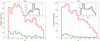 |
Fig. 1. Redshift distribution of the sources in the input catalog of the CDFS (left panel) and of the UDS (right panel). The red histograms represent the sources with photometric and spectroscopic redshifts, the green histograms the sources with spectroscopic redshifts from the literature. The inserts show the redshift distributions of the Lyα-emitting galaxies selected from the VANDELS database and used in this work. |
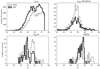 |
Fig. 2. Magnitude distribution of sources with photometric (upper left), spectroscopic redshifts from the literature (upper right), from VANDELS (lower left), and of the Lyα-emitting galaxies selected from the VANDELS database (lower right) in the CDFS (weak line) and in the UDS (strong line). |
3.2. Running the algorithm
Once the input catalog is defined, the algorithm works as follows. The entire survey volume is first divided into a grid of cells. Each grid cell is characterized by a position in the right ascension (ra), declination (dec), and redshift (z) space, according to its location in the survey volume, and by the same size Δra, Δdec, and Δz in the three directions. The number of galaxies from the input catalog in each cell depends on the density of galaxies in our field and on the cell dimension. Some cells may be empty, some can contain more than one galaxy.
To measure local densities, the three dimensions of each cell of the initial grid are increased in size by steps of Δra, Δdec, and Δz, and the code counts the number of galaxies within the increased volume of the cell. The density associated to that cell is then defined as ρN = N/VN, where VN is the comoving volume which includes the N nearest neighbours. The value ρN is also the density associated to the galaxies contained in that cell in the initial regular grid. Then the code studies the ρN values in the field, detects and extracts overdense structures in the 3D space. This procedure is performed with a SExtractor (Bertin & Arnouts 1996) approach. The code measures the mean and the standard deviation of the local densities in each redshift bin, applying a 2σ clipping in an iterative way. It extracts as overdensities the regions with densities larger than a certain THRESHOLD (defined in standard deviations above the mean local density), comprising a minimum number of cells from the initial regular grid (MIN_CELL), and a minimum number of galaxies (MIN_obj).
We use two sets of configuration parameters. The first set is related to the calculation of local densities; the second one is related to the detection and extraction of overdensities. We start with the parameters described in the papers cited at the beginning of Sect. 2. We define the first set as follows. The volume of a cell in the starting grid is defined as Δra × Δdec×Δz. We adopt ΔA = Δra = Δdec = 3 arcsec and Δz = 0.02. These values correspond to 75 cKpc (spatial direction) and 30 cMpc (redshift direction) at z = 2 considering our adopted cosmology. The extension of the cells depends on the positional accuracy and is characterized by a parallelepiped volume, elongated towards the redshift direction. The choice of Δz is related to the photometric redshift accuracy, 0.02 × (1 + z), which corresponds to ∼0.1 at z > 2. We fix the maximum cell length in the spatial directions to be 15 arcsec (380 cKpc at z ∼ 2) and to be 2 × Δz × (1 + z) in the redshift direction to avoid infinitely elongated cells with unphysically-low local densities (details can be found in Salimbeni et al. 2009). Also, we fix N = 10 and we verify that we do not obtain significant differences when we vary N from 10 to 20. In the case that ten sources are not counted after reaching the maximum size of a cell, the density is calculated from the number of sources contained in the cell of maximum size. We define MIN_CELL = 10 as previously optimized in Trevese et al. (2007), THRESHOLD = 6, and MIN_obj = 5 or 10 (at 3 < z < 4 or 2 < z < 3, respectively). These values are tested on our data and with mock galaxies (see Sect. 4), and they allow us to recover the structures previously identified at z ≃ 2.3 by Salimbeni et al. (2009). The choice of a lower MIN_obj value at z > 3 is justified by the fact that the number of sources in our input catalog decreases by a factor of 2 going from z ∼ 2.5 to z ∼ 3.5 (Fig. 1).
3.3. Identification of overdensities
In Fig. 3, we show the average of the local densities associated to every galaxy of the input catalog (⟨ρ⟩) as a function of redshift. The density, averaged over the entire field, is expressed as the number of galaxies per Mpc3 and decreases as the richness of sources in the input catalog declines. We are studying small-size areas, so we expect to see overdensities diffuse all over the field. The structures embedded in these diffuse overdensities are expected to have redshift peaks corresponding to the ones in the ⟨ρ⟩ vs redshift function (e.g., Trevese et al. 2007; Salimbeni et al. 2009). The code outputs the list of extracted overdensities together with the position in right ascension, declination, and the redshift of their highest signal-to-noise density peak.
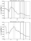 |
Fig. 3. Mean local density versus redshift for the CDFS (upper panel) and for the UDS (lower panel) shown as dashed solid curves. The mean corresponds to the average of the local density values in each bins of Δz = 0.02, after the application of sigma clipping, as explained in the text. Vertical solid lines represent the redshifts of the detected overdensities. In the lower panel, vertical dashed lines correspond to two slightly lower-threshold overdensities at z ∼ 2.8 (THRESHOLD = 4 instead of 6). |
Among the overdensities in the output list, we select a subsample of them characterized by dense cores. These are expected to be the most reliable structures (see also the test with the mock catalogs in Sect. 4). We consider the local densities associated to all the galaxies of the input catalog, we focus on the sources in bins of 0.1 redshifts (for instance at 1.95 ≤ z ≤ 2.05 or 2.05 ≤ z ≤ 2.15, and so on), and we calculate the average and the standard deviation of their associated densities (ρm01 and σm01). We identify as dense cores any region inside an overdensity with at least a given number of galaxies with associated densities larger than ρm01 + 2 × σm01, and contained in a certain circular projected area, where the number of galaxies is five (three) at z ∼ 2.5 (z ∼ 3.5) according to the number of sources in the input catalog (Fig. 1) and the radius of the circular area varies between 3.5–7 cMpc at z ∼ 2 and 4.5–8 cMpc at z ∼ 3. The choice of these values of radii is supported by simulations. Franck & McGaugh (2016) developed a method to identify the most massive protoclusters at z > 2 and investigated which volumes must be inspected to find them. While the most massive clusters have radii of the order of a few Mpc at z = 0, the protoclusters that would evolve into them are much more extended. By studying the Millennium simulation (Springel et al. 2005), Chiang et al. (2013) found that the effective radius of the progenitors of local clusters with masses of the order of 2 × 10¹⁴ M⊙ is 3.5 (4.5) cMpc on average at z ∼ 2 (z ∼ 3), while more massive clusters with masses larger than 1015 M⊙ can have effective radii up to 7 (8) cMpc at the same redshifts. With the aforementioned parameter choices, we expect to be able to identify the progenitors of z = 0 clusters with the lowest, but also the highest expected effective sizes.
We identify 22 overdensities at 2 < z < 4 (Sect. 5); we recover the structures found by Salimbeni et al. (2009) at z ∼ 2.3 with our same algorithm (Fig. A.1) and the dense structure detected by Forrest et al. (2017) at z ∼ 3.5 (Fig. A.4). Our final list of identified overdensities does not contain some of the dense regions found by Franck & McGaugh (2016) and Kang & Im (2015), which, however, are located in the positions of high-density peaks recognized by our algorithm (Figs. A.1, A.4, and A.5).
4. Algorithm performance on simulated galaxies
Trevese et al. (2007) tested the reliability of our algorithm in detecting clusters of various types and redshifts. They simulated galaxies of reasonable magnitude and distribution, and clusters of various richness numbers. They showed that a richness-0 cluster (Abell 1958) was detected with acceptable contamination up to z = 1 at a magnitude limit of 25 and it was still visible at z = 2 in a survey with magnitude depth of 27. Also, they calculated that it was possible to separate aligned clusters when their difference in redshift was larger than 0.15. By increasing the detection threshold of the algorithm, they showed it was then possible to separate overdensities with initially unseparated multiple peaks. Furthermore, Salimbeni et al. (2008) showed that our algorithm allows us to preserve high purity even for the smallest structures at z = 2.5. The comoving volume probed by VANDELS is larger than that studied in the previous papers, so we could expect to detect structures even of the highest numbers of richness. Also, the images VANDELS is based on are at least one magnitude deeper than the ones studied in the previous papers. Therefore, we could expect reliable performance of our algorithm at redshift up to 4. In this work, to check the performance of the algorithm in detecting overdensities in our current data, we make use of mock catalogs of VANDELS observations.
We first use the mock catalogs as an ideal Universe in which all the galaxies have secure redshifts and we identify overdensities. As described in the previous section, our code is designed to detect overdensities which are not necessarily either virialized or bound structures. To perform the identification of the overdensities, we generate an input catalog with the same magnitude cuts used for the real data and we run our code without considering photometric redshift uncertainties. We call this first run the fiducial-run and the identified overdensities are the fiducial-run overdensities. Then we apply photometric uncertainties to a given fraction of redshifts in the mock input catalog and compare the properties of the overdensities characterized by photometric-redshift uncertainties with the fiducial-run overdensities.
4.1. Mock of VANDELS observations
The VANDELS mock catalog is created from the GAlaxy Evolution and Assembly (GAEA) semi-analytic model (Hirschmann et al. 2016), embedded in the dark matter Millennium simulation. This model represents an evolution of the De Lucia & Blaizot (2007) code. The dark matter merger trees are extracted from the Millennium simulation (Springel et al. 2005). This is a cosmological N-body, dark-matter only simulation that follows the evolution of 21603 particles of mass 8.6 × 10⁸ h−1 M⊙ within a comoving box of 500 h−1 Mpc on a side. Dark matter haloes are identified using a standard friends-of-friends algorithm (e.g., Press & Davis 1982; Davis et al. 1985) with a linking length of 0.2 in units of the mean particle separation. The most-massive self-bound subhalo in a friends-of-friends group is its main subhalo, which contains a ‘central galaxy’.
From GAEA outputs, we generate light cones as described in Zoldan et al. (2017). The light-cone galaxies have all the observational properties we consider for the VANDELS galaxies, such as dust-dimmed magnitudes in U, B, V, HST ACS_F775W, i, z, J, HST WFC3_F160W-band filters and observed redshift (including peculiar velocities), in addition to virial mass, virial radius, virial velocity, and star-formation rate directly coming from the model.
To mimic the observations in the CANDELS (extended) area, we apply the magnitude cut of isel = 27.5 (isel = 26.1) to the mock catalog. The i-band distributions in the data and in the model are consistent down to the faintest considered flux and the mocks are complete down to the magnitude of the sample.
No treatment of Lyα radiation is included in the GAEA model. Therefore, it is just used to check the performance of our code in detecting overdensities of galaxies and the effect of photometric redshift uncertainties, but not to verify the observed physical properties of Lyα emitters.
4.2. Fiducial run on mock galaxies
After applying the same magnitude cuts as for the VANDELS input catalog, we build the fiducial run. The redshifts of the mock galaxies include peculiar velocities (zobs), but they are not affected by uncertainties as large as those from photometric redshifts. Therefore, to estimate the local densities we set a narrow width in the redshift direction (Δz = 0.005) for the cells of the initial regular grid. Also, we require THRESHOLD = 7 and MIN_obj = 10−5 (at z ∼ 2.5 and z ∼ 3.5, respectively) to be able to detect dense regions. These detection parameters allow us to identify density peaks that contain massive central galaxies (with virial masses larger than 1012 M⊙) and to take into account the fact that the number of galaxies decreases by at least half from redshift 2 to 3.
Our algorithm detects overdensities by linking together more than one bound or virialized structure as identified by the friends-of-friends algorithm in the simulation and more than one massive central galaxy. We perform a merger tree analysis of the mock structures in the light-cone till z = 0 and we find that 97% of the detected overdensities are still identified as such at z = 0. To better understand the properties of the overdensities we identify in the fiducial run, we consider the total number of members, the standard deviation of the redshifts of the members, the mean and maximum value of the distance of the members with respect to the highest-density peak (Fig. 4).
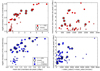 |
Fig. 4. Properties of the overdensities detected among the mock galaxies with isel ≤ 27.5 at 2 < z < 3 (red) and 3 < z < 4 (blue). The properties of the fiducial run overdensities (2 < z < 3FID and 3 < z < 4FID) are shown as dots and the properties of the overdensities detected after including zphot errors (mimicking the VANDELS data) and adopting THRESHOLD = 6 (2 < z < 3TH6 and 3 < z < 4TH6) are shown as stars. The leftpanels show the total number of members versus the mean distance between the members and the highest-density peak, the rightpanels show the maximum distance between the members and the highest-density peak and the standard deviation of the observed redshifts in velocity [c × stdev(zobs)]/[1 + mean(zobs)]. The fiducial-run overdensities missed after applying photometric uncertainties are indicated with black circles around the dots (missed). The ‘fake’ overdensities at z ∼ 3 (3 < z < 4TH6fake), not detected in the fiducial run, are shown as squares. To read this figure, we remind that each star (recovered overdensity) corresponds to a dot (fiducial-run overdensity) without black circle. The overdensities detected among the mock galaxies with isel ≤ 26.1 share the same properties of the ones detected among the mock galaxies with isel ≤ 27.5. |
The overdensities detected at 2 < z < 3 tend to be larger than those detected at 3 < z < 4. In fact, the maximum distance between the overdensity members and the location of the highest-density peak is on average 6.3 cMpc at z ∼ 2 and 3.5 cMpc at z ∼ 3. They also tend to be composed of a larger number of members. The standard deviation of the observed redshifts in velocity [c × stdev(zobs)]/[1 + mean(zobs)] is of the order of 1000 km sec−1 and it can be up to 3000 km sec−1 both in the lower and in the higher redshift bins. The overdensities that contain at least five massive central galaxies are the largest among all.
4.3. Effects of observational uncertainties
To simulate the conditions of real observations, we perturb the observed redshifts of the mock galaxies. Less than one fifth of the galaxies in the VANDELS input catalog have reliable spectroscopic redshifts. About 85–90% of the sources only have photometric redshifts. The number of photometric redshifts dominates that of spectroscopic redshifts and a ∼15% (in the CDFS) rather than a ∼10% (in the UDS) of spectroscopic redshifts equally contribute to the detection of overdensities. Therefore, we perturb the observed redshifts of a random 85% of the mock galaxies. The mock perturbed redshifts are obtained adding an error extracted from a Gaussian distribution centered on the unperturbed redshift and with sigma equal to the photometric redshift error. As we can see in the Table 5 of Pentericci et al. (2018b), the photometric redshift uncertainty has a weak dependence on magnitude and so the treatment of the photo-z errors is realistic enough for our purpose. The availability of a robust spectroscopic redshift can be magnitude dependent. However, the magnitude of the galaxies for which we have spectroscopic redshifts from VANDELS can be much fainter than that from other surveys and we verify that choosing the 15% of unperturbed redshifts only among the brightest galaxies does not change our results.
We, then, set the parameters of our code to account for the inclusion of redshift uncertainties. We use cells wider in the redshift direction than for the fiducial run case (Δz = 0.02) and ΔA = 3 arcsec as for the real data. We try three different values of THRESHOLD and check the fraction of recovered overdensities. The THRESHOLD values explored are lower than the value adopted in the fiducial run to account for the fact that the structures become more spread out due to the inclusion of photometric-redshift uncertainties. We also calculate the fraction of “fake” detections, i.e. the ones detected by setting the code parameters as for the real data, but not detected in the fiducial run. In Table 1, we report these fractions for THRESHOLD = 5, = 6, and = 7. To estimate these fractions, we assume that a recovered detection is real if it contains at least the highest-density peak of a fiducial-run overdensity.
Fraction of recovered and fake overdensities.
With THRESHOLD = 6, we obtain the best trade-off between recovered fiducial-run overdensities and low number of fake detections (Table 1), even for the case with isel ≤ 26.1. With the same uncertainties and magnitude cut as for the real data, we detect 68% and 63% of the fiducial-run overdensities at 2 < z < 3 and 3 < z < 4, respectively.
As we can see in Fig. 4, at THRESHOLD = 6 the spatial size of a recovered overdensity (expressed as the maximum separation between the overdensity members and the overdensity highest-density peak) is smaller than that of the corresponding overdensity detected in the fiducial run. The difference in spatial size is more evident for the overdensities at z ∼ 2 (1.8 cMpc on average compared to 6.3 cMpc on average for the fiducial run) than at z ∼ 3 (2.5 cMpc on average versus 3.5 cMpc on average for the fiducial run), where the number of members is also much more comparable than at z ∼ 2. The difference in size along the redshift direction is larger for the overdensities at z ∼ 3 (2500 km sec−1 on average versus 900 km sec−1 on average for the fiducial run) than at z ∼ 2. This could happen because when photometric redshift uncertainties are introduced, we see two effects: several peaks can be detected as disconnected structures and also very close pairs of peaks can be merged in a single, larger structure. The first effect is likely caused by galaxy members moving in redshift bins due to the errors. The second is caused by the larger smoothing of the distribution due to the introduction of the errors. The standard deviation of the observed redshifts of the galaxies of a recovered overdensity can be twice that of the fiducial-run overdensity (right panels of Fig. 4). This is an effect of the inclusion of the photometric redshift uncertainty.
In terms of spatial and redshift sizes, there are no clear differences between the fiducial-run structures that are missed and those that are recovered when setting the parameters to those used on the real data. The three fake detections at z ∼ 3 have less than ten members and a standard deviation of the observed redshifts larger than 1000 km sec−1. One of them (Nmembers = 33) is located at the border of the field.
This test on the mock galaxies demontrates that the largest uncertainty in detecting overdensities is given by the large number of photometric redshifts, rather than spectroscopic ones. To recover the fiducial-run overdensities and account for photometric-redshift uncertainty, we increase the cell size in the redshift direction. After including photometric-redshift uncertainties, our algorithm is able to identify mainly the highest-density peaks of the fiducial-run overdensities. The maximum distance between the members and the highest-density peak is of the order of 2 cMpc both at z ∼ 2 and at z ∼ 3 on average. The spatial size of the overdensities detected after the inclusion of zphot errors is more similar to that of the fiducial run at z ∼ 3 than at z ∼ 2, but the size along the redshift direction changes much more at z ∼ 3 than at z ∼ 2.
5. Properties of the overdensities identified in the CDFS and in the UDS
With the scope of studying the properties of star-forming galaxies, and in particular Lyα emitters, as they relate to their environment, we use the 3dv4 algorithm to detect overdensities. To run the algorithm, we chose the set of parameters reported in the previous sections (Δz = 0.02, ΔA = 3 arcsec, THRESHOLD = 6, MIN_obj = 10 and 5 at 2 < z < 3 and at 3 < z < 4, respectively) and we identify 22 overdensities, 13 in the CDFS and nine in the UDS.
In the following section, we describe the properties of the identified overdensities. We explain the observational properties we consider for the analysis in Sect. 5.1, then we qualitatively describe the most interesting overdensities (composed of more than one density peak, containing more than one spectroscopic redshifts), including the ones with Lyα emitters (Sect. 6) as members.
5.1. Observational properties of the identified overdensities
To characterize the observational properties of our overdensities, we determine the number of members, their redshift distribution, their physical properties, the dispersion velocity, and the overdensity total mass. For the majority of the overdensities, at least two members have spectroscopic redshifts. However, one and four structures, respectively in the CDFS and in the UDS, are defined solely by photometric redshifts.
Even if the overdensities tend to be elongated in the redshift direction, to calculate their volumes we adopt the formula of a sphere with radius equal to the mean member-to-member distance (Rmeandist), 4/3 π . For each overdensity redshift range, we define a corresponding field, which is composed of galaxies outside the area occupied by the overdensity, with density within ±3σ around the average local density (< ρ>, see Sect. 3.3). To estimate the number of galaxies of the field in a volume equal to the volume occupied by the overdensity, we count the number of field galaxies in a spherical volume centered at more than 2.5 cMpc8 away from the center of the overdensity and with the same Rmeandist radius of the overdensity. We repeat the calculation of the number of field galaxies in nine spherical volumes located at nine different centroids and we take the median value.
For the overdensities clearly composed of more than one peak in the spectroscopic-redshift distribution, we estimate the location and the scale of each peak, by following the formalism described in Beers et al. (1990). We calculate the location of the center of each peak with the biweight estimator and their width with the biweight scale estimator and the gapper scale estimator (Wainer & Thissen 1976). The former mainly takes into account the difference between the redshifts of members and the median redshift of the structure, the latter the redshift difference between members. To derive the scale estimator via the gapper method, we place an upper limit on the maximum velocity difference with respect to the central one of ±1500 km sec−1 (we remind the reader that one of the largest velocity dispersions measured for a cluster of galaxies is 1200 km sec−1 for the Coma cluster, Zabludoff et al. 1993).
We perform a bootstrap with replacement technique to estimate the uncertainties of the dispersion velocities.
We estimate the total mass, M, associated with our identified overdensities as that proportional to the matter overdensity (see Steidel et al. 1998; Cucciati et al. 2014; Lemaux et al. 2014). We list here some of the equations used to derive M, additional details can be found in the cited papers. M is defined as
 (1)
(1)
where ρ0 is the comoving mean density of the Universe (=Ωmρ0crit = 4.079 × 10¹⁰ M⊙ cMpc−3, given the adopted cosmology), δm is the matter overdensity in the structure, and V is the volume occupied by the overdensity in real space. For each overdensity, we estimate noverdensity as the number of members divided by the observed overdensity volume and nfield as the median number of the field galaxies in the redshift range of the overdensity and in a volume equal to the observed volume of the overdensity. Hence, the matter overdensity is proportional to the galaxy overdensity as
 (2)
(2)
where δgal=(noverdensity − nfield)/nfield, C relates the volumes in real (V) and observed space (Vobs) and depends on the adopted cosmology through f(z) = Ωm(z)4/7.
 (3)
(3)
such that V = Vobs/C (where Vobs is in comoving coordinates), and b is a bias factor ranging from 2 to 4 at 2 < z < 4 (Durkalec et al. 2015). We do not report mass estimates for the overdensities composed of a large number of multiple peaks nor for the overdensities with zero spectroscopic redshifts.
Given the redshift of a structure and δgal, Chiang et al. (2013) simulations provide a prediction of the kind of z = 0 clusters the overdensities may evolve to, either a Fornax-type (with 1.3−3.0 1014M⊙), or a Virgo-type (with 3−10 1014M⊙), or a Coma-type (with > 1015M⊙) cluster at z = 0. For example, we could expect that a protocluster at z ∼ 2 with δgal = 4(6) could be progenitor of a Virgo(Coma)-type cluster at z = 0. It can also happen that high-z overdensities may not be able to assemble a virialized cluster by z = 0. We use these simulation results to determine the fate of our identified overdensities in the next section.
To understand the stage of evolution of an overdensity and its members, we study rest-frame U − V color, stellar mass (M*), and the specific star-formation rate (sSFR = SFRSED/M*) of the structure members. The rest-frame U and V magnitudes correspond to the rest-frame absolute magnitudes at 3670 Å and 5500 Å, respectively, obtained assuming a 200 Å-wide tophat filter on the best-fit SED template. The rest-frame U − V color resembles the observed-frame J − K color, frequently used at z ∼ 2 to define the protocluster red sequence (Stott et al. 2012; Willis et al. 2013; Strazzullo et al. 2016) of evolved, possibly passive galaxies.
We compare rest-frame U − V color, M*, and sSFR of the overdensity members with those corresponding to the galaxies in the field (Appendix B) and we estimate if the set of quantities of the members and the field galaxies are drawn from the same distribution by using a KS test. For reference, the rest-frame U − V colors for passive galaxies in the VANDELS photometric catalog is about 1.7, while it is ∼0.62 for star-forming galaxies at z ∼ 2.8, and ∼0.63 for LBGs at z ∼ 3.4 (following the definition of the VANDELS galaxy populations in Pentericci et al. 2018a).
We also consider the rest-frame color-color diagram composed of the U − V and V − J colors to investigate any possible physical vs morphological property trend among the galaxies of each structure (Strazzullo et al. 2013; Newman et al. 2014). Given the availability of the morphological catalogs from CANDELS (van der Wel et al. 2012), we study the morphology of the overdensity members in terms of GALFIT Sersic index and axis ratio. The rest-frame J magnitude corresponds to the rest-frame absolute magnitudes at 12 500 Å, assuming a 200 Å-wide tophat filter. In Appendies C and D, we show all these trends and we comment them in detail only for the most notable structures discussed in Sect. 5.2. We do not report morphological considerations for the galaxies located in the extended areas of the CDFS and of the UDS.
5.2. Overdensities identified in the CDFS and in the UDS
The main observational properties of the 22 identified overdensities, such as the number of members estimated by our algorithm and the number of members with spectroscopic redshifts, are presented in Table 2. The redshift distributions of each identified overdensity are shown in Figs. 5 and 6. In Appendix A, we show the regions occupied by our 22 identified overdensities, together with the location of structures identified by Kang & Im (2015), Franck & McGaugh (2016) in the CDFS. In Appendix B, we show the space distribution of each of the identified overdensity; in Appendix C and D, we show the physical properties of the most interesting overdensities described here below.
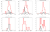 |
Fig. 5. Redshift distribution of the galaxies in the overdensities identified in the CDFS. The red histograms include both spectroscopic and photometric redshifts, while black histograms only the spectroscopic ones. The histogram bin is 0.02 in redshift. Some of overdensities are likely composed of more than one density peak. |
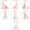 |
Fig. 5. continued. |
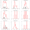 |
Fig. 6. Same as Fig. 5 for the overdensities identified in the UDS. Some of the overdensities could be composed of more than one density peak, such as the structure at z ≃ 2.33. |
Characteristics of the structures identified in the CDFS and in the UDS.
We provide a qualitative description of the overdensities, leaving a more quantitative analysis for another paper. Generally, the overdensities we identify are composed of more than one peak in space and present typical sizes of the order of 1–4 cMpc, comparable with the sizes of the structures detected in the mock catalogs. However, the maximum distance between the members and the highest-density peak is of the order of 3 cMpc at both z ∼ 2 and z ∼ 3 on average. The size in redshift space, expressed as [c × stdev(z)]/[1 + zpeak], is 4000 km sec−1 at both z ∼ 2 and z ∼ 3 on average, even twice larger than the value calculated for mock galaxies. This can indicate that density peaks, overlapping in redshift space, tend to be interpreted as unique structures by our code, more than what was observed in the case of mock galaxies to which we applied photometric redshift uncertainty independent of environment. Spectroscopic follow-ups of overdensity members are needed to better delineate the redshift-space characteristics of the detected overdensities.
In Appendix C, we also report the Kolmogórov-Smirnov (KS) tests performed to evaluate if stellar masses, sSFRs, and rest-frame U − V colors of the members and field galaxies are drawn from the same distribution. We usually find that we can reject the null hypothesis that these three physical properties of the members and field galaxies are drawn from the same distribution at least at 2σ (we will highlight in the following the cases in which, instead, we can not reject the null hypothesis).
However, we can not identify a red sequence from the rest-frame U − V color of the members of any of our overdensities.
According to the value of the highest-density peak and the redshift of our overdensities, we find that they could be progenitor of Fornax-type clusters at z = 0, which would virialize at 0.2 < z < 1. We will highlight in the following the cases in which the total mass estimate is not consistent with the value expected for a Fornax-cluster progenitor at z ∼ 2−4 (Chiang et al. 2013)
Overdensity at z = 2.29 in the CDFS. This is a large overdensity (in space and redshift), probably composed of more than one main peak (Fig. B.1). As we can see in Fig. A.1, a structure detected by Kang & Im (2015) is included in our overdensity region. One of the main peaks is in the center of the entire overdensity. From this position, filamentary structures depart along the RA direction.
As we can see in Fig. C.1, the bluest members with the highest sSFRs have morphologies consistent with disk galaxies. However, the members with the lowest sSFRs can have a variety of morphologies (Sersic index 0 < n < 5). Even if we can not identify a red sequence from the rest-frame U − V color, there is a tail of field galaxies with U − V colors redder than the members. The mass of the overdensity derived from the matter density is of the order of 9 × 10¹² M⊙.
Overdensity at z = 2.30 in the CDFS. This overdensity overlaps with the one found in Salimbeni et al. (2009) at z ∼ 2.3 (Fig. A.1). It is composed of one main density peak. A secondary peak is located to the north of the main one (Fig. B.2). There are galaxies with sSFRs much higher than the mean value towards the center and also in the outskirts of the overdensity (Figs. B.2 and D.1).
Stellar masses, sSFRs, and rest-frame U − V colors of the members occupy the same parameter space as field galaxies (Figs. C.1 and D.1). A KS test shows that we can not reject the hypothesis that the distributions of rest-frame U − V colors are drawn from the same distribution. The members with spectroscopic redshifts are more massive, brighter in the optical than the other members, and some of them are the reddest members in terms of rest-frame U − V color. The members with the highest sSFRs have a variety of morphologies in terms of Sersic index and axis ratio (Fig. D.1). The mass of the overdensity derived from the matter density is 1 × 10¹³ M⊙.
Overdensity at z = 2.80 in the CDFS. This overdensity is composed of one main peak (Fig. B.6) and a tail. The galaxies composing the main density peak have a large spread in sSFR values and morphologies (Figs. B.6 and D.2).
Stellar masses, sSFRs, and rest-frame U − V colors of the members expand the same range of values of the galaxies in the field (Figs. D.2 and D.2). A KS test shows that we can not reject the null hypothesis that those quantities are drawn from the same distribution. The mass of the overdensity derived from the matter density is about 4 × 10¹² M⊙. According to the simulations in Chiang et al. (2013), this structure could be progenitor of a Fornax or Virgo-type cluster at z = 0, which would not be virialized before z = 1.6.
Overdensity at z = 3.17 in the CDFS. This overdensity occupies a large area of CDFS at z ∼ 3.2. Our algorithm identifies a region of the space with a high concentration of galaxies distributed around at least three main density peaks (Figs. 5 and B.7). Two of the Lyα-emitting galaxies discussed in the next section are members of this overdensity.
The density peak at dec = −27.76° is mainly composed of galaxies with sSFRs < 6 × 10⁻⁹ yr−1, rest-frame U − V colors redder than the field galaxies, and morphologies consistent with that of elliptical galaxies (average Sersic index equal to 2.4; Figs. C.3 and D.2). Therefore, at that declination the member galaxies are in an evolved state with respect to field galaxies, despite the fact that the stellar mass distribution of the members and field galaxies can be drawn from the same distribution (KS = 0.04, p = 0.72).
The spectroscopic redshift distribution shows three peaks, at 3.0 ≤ zspec < 3.3, at 3.3 ≤ zspec < 3.6, and at 3.6 ≤ zspec < 3.9, respectively composed of 14, 13, and seven sources. As we can see in Fig. 7, the lowest redshift peak traces the left side of the overdensity, while the other peaks mainly trace the right side of the overdensity. The highest-redshift peak could be a tail of random alignment. This could indicate that this overdensity is composed of two structures, unlikely to be connected because of the difference in redshift and so unlikely to evolve all together in a cluster at lower redshift. By using the bweight and gapper methods (Sect. 5.1), we estimate the dispersion velocity of the galaxies in the three redshift peaks. The redshifts of the three peaks are 3.08 ± 0.01, 3.49 ± 0.01, and 3.69 ± 0.01. The dispersion velocities are 3620 ± 1030, 2940 ± 660, and 1550 ± 290 km sec−1 if calculated with the bweight method and 1200 ± 290, 1080 ± 420, and 1090 ± 410 km sec−1 if calculated with the gapper method. The difference in these values is due to the different upper limits in velocity applied in the two methods. In an upcoming paper, we will study in detail the galaxies of this overdensity and its fate to lower redshift.
 |
Fig. 7. Density map of two peculiar overdensities. The structures at z = 3.17 in the CDFS is shown in the leftpanel, the structures at z = 2.33 in the UDS is shown in the rightpanel. Red diamonds correspond to the spectroscopic members within the lowest redshift peaks, blue diamonds to the intermediate redshift peaks, green diamonds to the highest redshift peaks as seen in Fig. 6 and explained in the text. |
Overdensity at z = 3.54 in the CDFS. This overdensity is composed of two peaks (Fig. B.11), one of the two contains galaxies with very low sSFRs relative to the average. One of the Lyα-emitting galaxies discussed in the next section is a member of this overdensity. The mass of the overdensity derived from the matter density is about 1 × 10¹³ M⊙.
Overdensity at z = 3.55 in the CDFS. This overdensity is elongated along the RA direction and it is composed of two main peaks (Fig. B.12). One of the Lyα-emitting galaxies discussed in the next section is a member of this overdensity. The overdensity overlaps with the structure found by Forrest et al. (2017), detected thanks to the discovery of several [OIII]+Hβ-emitting galaxies (Fig. A.4). Members with sSFR values larger than the average are located either in the core or in the outskirts of the overdensity (Figs. B.12 and D.3). The mass of the overdensity derived from the matter density is about 2 × 10¹³ M⊙.
Overdensity at z = 2.33 in the UDS. This overdensity occupies a 6′x15′ area of the UDS at z ∼ 2.3 (Fig. A.5). Our algorithm identified a region of space with a high concentration of galaxies distributed around four main density peaks (Fig. B.14). It is not entirely unusual to identify overdensities of this extent. Balestra et al. (2010) also discovered several structures in the central part of CDFS, such as those at z ≃ 2.3 and z ≃ 2.6, spatially extended over their entire surveyed area (15 Mpc).
A variety of physical properties characterize the galaxies of the overdensity. The density peak at dec = −5.18° is mainly composed of galaxies with sSFRs < 3 × 10⁻⁹ yr−1 (the average value among all the members), but a variety of morphologies (Figs. B.14 and D.4). The members with spectroscopic redshifts are the brightest and most massive (Fig. C.4) among all.
The spectroscopic redshift distribution shows three peaks, at 2.00 ≤ zspec < 2.27, at 2.27 ≤ zspec < 2.37, and 2.37 ≤ zspec < 2.50, respectively composed of 92, 57, and 16 sources. As we can see in Fig. 7b, the spectroscopic redshifts roughly trace the position of the highest-density regions. In particular, the intermediate and highest redshift peaks trace the overdensity peak at RA = 34.4°. Therefore, the identified overdensity could be composed of a main structure at z ≃ 2.3, a filament at lower redshift, and a tail at higher redshift.
By using the bweight and gapper estimators (Sect. 5.1), we estimate the dispersion velocity of the galaxies in the thee main redshift peaks. The redshifts of the three peaks are 2.188 ± 0.004, 2.305 ± 0.003, and 2.401 ± 0.006. The dispersion velocities are 3700 ± 190, 1960 ± 210, and 2340 ± 480 km sec−1 if calculated with the bweight estimator, 2050 ± 210, 1070 ± 140, and 900 ± 210 km sec−1 if calculated with the gapper estimator.
Overdensity at z = 3.25 and RA = 34.52o in the UDS. This overdensity is composed of one main peak (Fig. B.15). The members with sSFRs more than twice above the average are located in the outskirts of the overdensity, and have a variety of morphologies (Figs. B.15 andD.4).
The stellar masses and sSFRs are consistent with those of the galaxies in the field. However, a KS test shows that we can not reject the null hypothesis that the distribution of rest-frame U − V colors of the members and field galaxies are the same (Figs. C.4 and D.4). Two of the Lyα-emitting galaxies discussed in the next section are members of this overdensity. Interestingly, their physical properties are consistent with the average properties of the other members. The mass of the overdensity derived from the matter density is 0.4 × 10¹³ M⊙.
Overdensity at z = 3.27 in the UDS. This overdensity is composed of one main density peak with a tail (Fig. B.17) in the RA-dec plain. One of the Lyα-emitting galaxies discussed in the next section is a member of this overdensity. Galaxies with sSFRs lower than the mean value of the overdensity are located either in the peak or in the tail and they tend to have morphologies consistent with disk-like galaxies (Sersic index n< 2, Figs. B.17 and D.5). The mass of the overdensity derived from the matter density is about 5 × 10¹² M⊙.
Overdensity at z = 3.65 in the UDS. This overdensity is composed of one main peak (Fig. B.20). Two of the Lyα-emitting galaxies discussed in the next section are members of this overdensity. One of them is located in the outskirts of the structure. Also, the two members with sSFRs more than twice above the average value are located in the outskirts of the overdensity.
The mass of the overdensity derived from the matter density is about 1 × 10¹² M⊙. The intensity of the peak overdensity and its redshift indicate that this structure could be progenitor of a massive Coma-type cluster at z = 0, which would virialize at 1.5 < z < 2.3. However, the mass we estimate at the current redshift is much lower than the value expected for a Coma-cluster progenitor at z ∼ 3.6 (Chiang et al. 2013). This could indicate that this structure will not be able to actually assemble at z < 3. We do not have enough supporting evidence to evaluate if the structure will fragment and evolve in several substructures.
5.3. Stage of evolution of the galaxies in the identified overdensities
Associations of galaxies at z > 2 have been identified in simulations (Chiang et al. 2013; Muldrew et al. 2015) and in observations (Castellano et al. 2007; Salimbeni et al. 2009; Kang & Im 2015; Franck & McGaugh 2016), and have shown a variety of properties (e.g., size, mass, number of members) and stages of evolution. Overdensities could be composed of massive and evolved galaxies, but we could be missing a given galaxy population, depending on the identification method and when our sample only includes a biased type of tracers. Moreover, to better identify overdensities and determine their structures, it is desirable to have a high spectroscopic coverage in observing fields larger than 10 cMpc on a side (Muldrew et al. 2015).
Some of the overdensities identified in this work are characterized by properties expected for high-density regions in the local Universe, such as members with low sSFRs in the cores and morphologies consistent with those of elliptical galaxies. However, the majority of the overdensities do not show rest-frame U − V, V − J colors, and optical magnitudes typical of virialized clusters at z < 1 (Willis et al. 2013).
To investigate the stage of evolution of the galaxies in the overdensities we detected at 2 < z < 3 and at 3 < z < 4, we show the average rest-frame U − V color (rest-frame (U − V)overdensity) as a function of redshift and the difference between the average color of the overdensity members and field galaxies (rest-frame (U − V)overdensity - rest-frame (U − V)field) as a function of rest-frame (U − V)overdensity (Fig. 8). The rest-frame (U − V)overdensity values are broadly consistent with the typical values of star-forming galaxies at z ∼ 2.8 and Lyman break galaxies at z ∼ 3.4 (Pentericci et al. 2018a). The rest-frame (U − V)overdensity color is independent of redshift for the structures studied here and it is of the order of 0.7 with a large scatter. It is worth noting that the colors of the structures detected in the CDFS and in the UDS are comparable with the values calculated for the overdensities detected in the mocks.
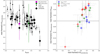 |
Fig. 8. Leftpanel: mean rest-frame U − V color of the galaxies in the 22 overdensities identified at 2 < z < 4 versus redshift of their highest-density peaks (big black diamonds). We, also, show mean color and mean photometric redshift for star-forming galaxies (big magenta squares) and Lyman Break galaxies (big green circles) as classified in Pentericci et al. (2018a) and for the structures detected in the mocks, in the fiducial run (small gray circles) and in the run with parameters as in the real data (small black circles). Rightpanel: difference between the mean rest-frame U − V color of the overdensity members and the mean rest-frame U − V color of field galaxies versus the mean rest-frame U − V color of the overdensity members. The color coding indicates the redshift of the highest-density peak of the identified overdensities, blue for z < 2.7, green for 2.7 ≤ z ≤ 3.3, and red for z > 3.3. The error bars correspond to the standard error of the means. As a reference, the rest-frame U − V color for a representative cluster at z = 0 is equal to 1.4 and that of field galaxies is 0.5. To derive these values, we assume that a z = 0 cluster contains a well defined red sequence with a dominance of E and S0 galaxies and that field galaxies are a blue population (Fukugita et al. 1995). |
The right panel of Fig. 8 shows that the typical galaxy members are not systematically redder than field galaxies. The difference between the rest-frame U − V color of the overdensity and its associated field galaxies is usually much less than 0.2, with a typical uncertainty of 0.06. For half of the overdensities, it is consistent with zero (less than 0.05, with a typical uncertainty of 0.05). There are ten overdensities for which the difference is 0.11 ± 0.07 on average. There is just one overdensity (the one at z = 4.01 in the UDS without spectroscopic redshifts) for which it is −0.23 ± 0.09. Therefore, the typical overdensity members are not that different from the field galaxies in terms of rest-frame U − V color. This is reflected in the properties discussed in the previous section as well.
6. Lyα emitters and environment
Useful insights on the properties of galaxies either in dense or in sparse environments could be provided by their Lyα emission. The Lyα emission of a star-forming galaxy is related to its recent star formation and it is sensitive to the interstellar (ISM) and circumgalactic medium (CGM) properties, such as HI content and distribution. The confinement or stripping of HI gas due to environmental effects could condition the evolution of the galaxy and also affect the distribution of its Lyα photons.
We select a sample of Lyα-emitting galaxies from the current VANDELS archive (LAEVs) and study their location with respect to the environment. As mentioned in Sect. 2, a LAEV is defined as a galaxy with EW(Lyα) > 0 Å measured in its VANDELS spectrum (e.g., Pentericci et al. 2018a,b; Marchi et al. 2019). We estimate the EW(Lyα) when the Lyα emission line is detected with a signal-to-noise ratio above 1.5 (to assure a large enough variety of Lyα strengths), assuming an asymmetric Gaussian-profile fit of the emission line above the continuum (see Eq. (3) in Guaita et al. 2017) and considering the flux density of the continuum between 1300 and 1400 Å rest-frame. The error bar on the EW(Lyα) measurement is obtained propagating the error on the integrated flux of Lyα and the rms of the continuum, where the error on the integrated flux is calculated from the equation given by Lenz & Ayres (1992) for a Gaussian fit. The error bars are larger for the Lyα emission lines detected with signal-to-noise ratio just above 1.5. In the CDFS (UDS) we consider 51 (80) galaxies at 3 < z < 4 with 1 < EW(Lyα) < 2 00 Å. Their Lyα equivalent width distribution is shown in Fig. 9. Due to their initial selection from drop-out galaxies, they do not all show large values of Lyα equivalent widths, as it is the case of narrow-band selected Lyα emitters (e.g., Guaita et al. 2010). The median EW(Lyα) of the LAEVs in overdense regions is 12 Å and of the LAEVs in the field is 17 Å.
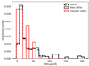 |
Fig. 9. Normalized Lyα equivalent width distribution of the Lyα-emitting galaxies selected from the VANDELS database (LAEVs). The dashed histogram corresponds to the entire sample of LAEVs. The thin black and red histograms are the distributions for the LAEVs located in the field and members of the detected overdensities (as explained in the text), respectively. |
Our LAEVs are VANDELS targets (Pentericci et al. 2018a), they are galaxies with zspec from VANDELS, and their location was not preselected in terms of density or environment. To study the location of galaxies with and without Lyα in emission with respect to environment and to study the relation between Lyα emission and environment, we compare the positions and physical properties of the LAEVs with those of the galaxies without Lyα emission all from VANDELS to avoid sample inhomogeneity (see Sect. 2.1).
To do this, we define three subsamples of galaxies: (a) all the galaxies in the input catalog (with either photometric or spectroscopic redshift, zphotspec); (b) the galaxies with spectroscopic redshifts from VANDELS, but without Lyα emission in their spectra (zspecV); (c) the LAEVs. Moreover, we define four different density category, and we measure the fraction of zphotspec, zspecV, and LAEVs in each environment with respect to the total number in a certain redshift bin.
The four density categories are defined as follows. The field (F) category is composed of galaxies with density within 3σ of the average local density and in the redshift bin of an identified overdensity; the transition (T) category is composed of galaxies with local density in between the field and the overdensities in the same redshift bin; the overdensity (O) category is composed of galaxies with density values consistent with an overdensity (6σ above the average local density), but that are not members of the identified overdensities, in the same redshift bin; and the overdensity-member (M) category is composed of galaxies that are members of the identified overdensity. The OM category is composed of galaxies in the O and M categories.
We consider the redshift bins of the identified overdensities and we count the number of zphotspec, zspecV, and LAEVs in each redshift bin. Then we count the number of galaxies per density category in each redshift bin. Finally, we measure the fraction of galaxies of a certain density category in a certain redshift bin as the ratio of the previously defined numbers.
In Table 3, we show the mean, the mean uncertainty, and the median of the fractions of zphotspec, zspecV, and LAEVs among the redshift bins of all the identified overdensities. The uncertainties on the mean quantities are calculated following the prescription in Gehrels (1986). In the case of statistically small samples of astrophysical events, they provide a method to calculate the lower and upper values of the confidence levels of a certain number of events (Eqs. (7) and (14) in Gehrels 1986). We choose the confidence levels corresponding to a 1σ limit in the case of Gaussian statistics (Sect. 1 and Tables 1 and 2 in Gehrels 1986).
Fraction of galaxies versus environment.
The fraction of the galaxies of the input catalog located in the field is 60%, being the fraction in transition and overdense regions 40%. The galaxies with spectroscopic redshifts coming from VANDELS are 3% of the total galaxies in the input catalog. About 70% of them happen to be in the field and only 4% are members of the detected overdensities (Table 3).
The LAEVs follow the location of the galaxies with zspecV. Therefore, our results indicate that, selecting a sample of galaxies unbiased in terms of environment, Lyα-emitting galaxies do not predominantly appear to be located inside overdensities. As we can see from the table, less than 2% of the LAEVs are members of the detected overdensities.
We separate the LAEVs in subgroups, based on EW(Lyα), stellar mass, and sSFR (see the following subsection). About 80% of the LAEVs with EW(Lyα) > 20 Å (typical equivalent width cut applied in narrow-band surveys of LAEs). The most massive LAEs (with stellar mass larger than the median value, LAEVs[M*> medM*]) and the ones with the smallest sSFR (with specific star-formation rate smaller than the median value, LAEVs[sSFR < medsSFR]) are located in the field in a lower fraction (66% and 71%, respectively). Among the LAEVs, 15% of the most massive are located in overdense regions.
6.1. Physical properties of the Lyα-emitting galaxies in the overdense regions
In Fig. 10, we study the physical properties of the LAEV sample. In comparison to typical narrow-band selected LAEs (e.g., Gronwall et al. 2007; Hagen et al. 2016), the LAEVs considered here, Lyman break galaxies by selection, have lower sSFRs (< 2 × 10⁻⁸ yr−1 versus values up to 10−7 yr−1) and are more massive [8.5 < log(M*/M⊙) < 10 versus values down to log(M*/M⊙) = 7]. However, these values of physical parameters are reasonable and in agreement with models of Lyα-emitting galaxies. For instance, Gurung-López et al. (2020) show the distribution of stellar mass and star-formation rate of Lyα-emitting galaxies from a model that incorporates Lyα radiative transfer processes in the interstellar and intergalactic medium (Gurung-López et al. 2019a), and that is implemented in the GALFORM semi-analytic model of galaxy formation and evolution (Lacey et al. 2016; Baugh et al. 2019). The distribution of stellar masses of Lyα-emitting galaxies at 2 < z < 3 extends from log(M*/M⊙) = 7 to 10, with a peak at log(M*/M⊙) = 9.0. According to the SFR distribution, the most probable value of the sSFR would be around 2 × 10⁻⁹ yr−1.
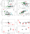 |
Fig. 10. Upper panels: LAEV physical properties with respect to the environment in the VANDELS fields. The LAEVs located in the identified overdensities and with EW(Lyα) > 20 Å are shown as red stars, the ones with EW(Lyα) < 20 Å are shown as green stars, the ones located in transition regions are shown as cyan circles and in the field as black circles. Dashed lines indicate the median values of sSFR, stellar mass, and EW(Lyα) = 20 Å of the entire LAEV sample. The physical properties we investigate are sSFR versus EW(Lyα) (upper left), stellar mass versus EW(Lyα) (upper right), dust reddening, Av, versus rest-frame optical magnitude (lower left), rest-frame NIR magnitude versus rest-frame UV magnitude (lower right). The squares with error bars represent the typical parameter uncertainties coming from the SED fitting (see the upcoming work on SED fitting parameters). Lower panels: median physical properties of the LAEVs and of all the galaxies in the input catalog located in overdensities (red symbols) and in the field (black symbols). The medians are presented as diamonds for all the galaxies in the input catalog and stars for the LAEVs. The error bars on the medians correspond to the uncertainties due to SED fitting. The physical properties we investigate are sSFR versus stellar mass (upper left), stellar mass versus distance to the highest-density peak (upper right) of the identified overdensities, dust reddening, Av, versus rest-frame optical magnitude (lower left), rest-frame NIR magnitude versus rest-frame UV magnitude (lower right). |
The upper panels of the figure show that 70%(30%) of the LAEVs with EW(Lyα) < 20 Å (> 20 Å) in overdense regions have sSFRs lower than the median value of the entire sample of LAEVs. All the low-EW LAEVs in overdense regions have stellar masses higher than the median value. Also, they tend to be brighter in the rest-frame UV magnitude. Typically, the LAEVs in overdense regions are more massive and have lower sSFR than the LAEVs in the field. Also, they are brighter in the rest-frame UV, optical, and NIR.
The average EW(Lyα) is 17 ± 5 and 35 ± 4 Å for the LAEVs in the identified overdensities and in the field, respectively (see also Fig. 9). However, the KS test shows that we can not reject the null hypothesis that the EWs in the overdensities and in the field are drawn from the same distribution. Some of the LAEVs in overdense regions have non-zero dust content (AvSED parameter, despite the large uncertainty we expect for the Av parameter), even though they have high Lyα equivalent widths.
We perform a KS test to compare the properties of the LAEVs in the identified overdensities and in the field. According to the test, we can reject the null hypothesis that masses, sSFRs, and rest-frame UV of LAEVs in the overdensities and in the field are drawn from the same distribution at more than 2σ ((KS, p)mass = (0.40,0.10); (KS, p)sSFR = (0.47, 0.03); (KS, p)restUV = (0.42,0.08)). The average stellar mass of the LAEVs in the identified overdensities is 9.6 ± 0.1 M⊙ and that of the LAEVs in the field is 9.25 ± 0.04 M⊙ in log scale (the median values are 9.6 and 9.2, respectively). The average sSFR is 6.0 ± 2.1 × 10⁻⁹ and 7.7 ± 0.7 × 10⁻⁹ yr−1, and the medians are 1.5 × 10⁻⁹ and 4.2 × 10⁻⁹ yr−1, respectively. The average rest-frame UV is −20.6 ± 0.2 and −20.3 ± 0.1 mags, and the medians are −20.8 and −20.3 mags, respectively.
As we can see from the plots in the lower panels of the figure, the LAEVs in overdense regions have stellar mass and sSFR consistent with the galaxies of the input catalog in overdense regions. However, they are brighter in the rest-frame UV and NIR. Even if the LAEVs studied here do not have all the physical properties of typical Lyα emitters, the ones in the overdensities share some physical properties of the galaxies we find in overdense regions and could provide information about the overdensities.
6.2. Spectroscopic properties of the Lyα-emitting galaxies in the overdense regions
The Lyα emission escaping a galaxy is sensitive to the properties of the ISM and of the CGM. Therefore, the information derived from the Lyα of the LAEVs may be used to infer the characteristics of the ISM and of the CGM of the galaxies in overdense regions. Moreover, theoretical predictions have shown that bright Lyα emitters reside in, and so could trace, more massive halos (e.g., Garel et al. 2015) on average. In this subsection, we study the spectroscopic properties of the LAEVs in overdense with respect to field regions, and we investigate if the Lyα emitters can be used to trace the environment characteristics.
In Fig. 11, we compare the Lyα flux and luminosity of the LAEVs in the identified overdensities and in the field. The median value of the L(Lyα) is 1.3 × 1042 (1.6 × 1042) erg sec−1 for the LAEVs in overdense (field) regions. The KS test shows that we can not reject the null hypothesis that the Lyα fluxes and luminosities of the LAEVs in overdensities and in the field are drawn from the same distribution ((KS, p)F = (0.22,0.78); (KS, p)L = (0.26, 0.58)). Therefore, in our sample, we do not observe a trend for which galaxies in overdense regions are significantly brighter in Lyα luminosity than in the field.
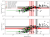 |
Fig. 11. Upper panel: Lyα flux vs Lyα equivalent width. lower panel: Lyα luminosity vs Lyα equivalent width. Green (red) stars indicate LAEVs in the identified overdensities with EW(Lyα) < 20 Å (EW(Lyα) > 20 Å), black dots indicate the LAEVs in the field. The vertical lines correspond to the mean (solid) and median (dashed) values of the EW(Lyα) of LAEVs in overdensities (red) and in the field (black). The horizontal lines correspond to the mean (solid) and median (dashed) values of the F(Lyα) and L(Lyα) of the LAEVs in the detected overdensities (red) and in the field (black). The shaded areas indicate the standard deviation of the means. The mean and median values of the F(Lyα) of the LAEVs in the detected overdensities and the median value of the F(Lyα) of the LAEVs in the field overlap. The mean and median values of the L(Lyα) is 1.4 ± 0.4 × 1042 and 1.3 × 1042 erg sec−1 for the LAEVs in the detected overdensities, while they are 2.9 ± 0.5 × 1042 and 1.6 × 1042 erg sec−1 for the LAEVs in the field. The median value of the LAEVs in the identified overdensities with EW(Lyα) < 20 Å (> 20 Å) is 7.4 × 1041 erg sec−1 (1.7 × 1042 erg sec−1). |
The shape of the Lyα emission line can provide information on the HI column density and kinematics (Verhamme et al. 2006; Guaita et al. 2017) of the emitting galaxy. Due to the interplay of dust and HI gas in the ISM and in the CGM, the Lyα emission line profile can present two peaks, one red shifted and one blue shifted with respect to the systemic redshift. The shift of the main red peak can be related to the HI column density and gas kinematics, such as stellar outflows. Radiative transfer models predict that the intensity of the blue peak and the separation between blue and red peak are also connected with the HI column density (Verhamme et al. 2015). Guaita et al. (2017) showed that the galaxies characterized by low HI column densities (NHI ∼ 1018 atoms cm−2) experience stellar-driven outflows with velocities, Vexp, of the order of a few hundreds of km s−1 and present spatially concentrated Lyα emissions. In the galaxies characterized by large HI column densities (> 1020 atoms cm−2), Lyα photons can be efficiently scattered even in the case of static media and can produce extended Lyα halos. However, more complicated geometries of the ISM or of the CGM could also provide interpretations of the NHI values.
Although VANDELS spectra are designed to achieve high signal-to-noise ratio, photospheric stellar absorption lines are intrinsically too weak in individual LAEV spectra to be used as tracers of the systemic redshift. In addition to this, nebular emission lines, such as CIII]1908 and HeII, are not detected in a statistically-meaningful subsample of the Lyα-emitting galaxies studied here (e.g., Marchi et al. 2019). Therefore, we are not able to derive gas kinematics information from the shift of low-ionization absorption lines and systemic redshift for the LAEVs. We can, however, stack the LAEV spectra centered on the Lyα wavelength to analyse the average shape and spatial extension of the Lyα emission.
In Fig. 12, we show the stack of the normalized 1D spectra of the LAEVs in overdense, transition, and field regions. The stacks are obtained from the rest-frame spectra, aligned to the highest-flux wavelength of the Lyα red peak. The stack of the galaxies in the identified overdensities shows a marginal blue peak, whose integrated flux is eight times smaller than that of the main red peak (see Table 4). The blue peak is clearly visible in the spectra of five of the nine sources. However, this blue peak is consistent with the continuum level at ∼1σ. In the lower panels of the figure, we show the best fit asymmetric Gaussian curves (see Eq. (3) in Guaita et al. 2017) of the three profiles. At the resolution of our data, the levels of asymmetry (A parameter) and the full width half maxima (FWHM parameter) of the three profiles are equivalent.
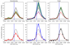 |
Fig. 12. Upper panels: stacks of the Lyα profiles of the LAEVs in the identified overdensities (leftpanel), transition (middlepanel), and field (rightpanel) regions. The green shaded areas indicate the standard deviation of the mean of the fluxes at each wavelength among all the LAEVs in a certain density category. The observed profiles of the LAEVs in overdensity (transition) (field) regions is shown in red (blue) (black) in every panel. The dashed-dotted lines show the median stacks. Lower panels: asymmetric Gaussian curves, best fits of the stacks (dots with errorbars) in the upper panels. In each panel, red is used for the LAEVs in the identified overdensities, blue for the LAEVs in transition regions, black for the LAEVs in the field. The best fits of the asymmetric Gaussian curves provide the following parameters (λ, FWHM, A) = (1215, 4 Å, 0.86), (1215, 3 Å, 0.95), and (1215, 3 Å, 0.83) for the left, middle, and right stack, respectively. |
Lyα integrated flux from the normalized stacked spectra.
In principle, the tendency of the galaxies in overdense regions to have low Lyα equivalent widths, high stellar masses, and low sSFRs could indicate that the LAEVs in overdense regions either are forming stars at a lower rate than the LAEVs in the field or they have already experienced intense star-formation phases. In addition to this, the presence of a blue peak may imply that the galaxies in dense environments are characterized by low NHI or lower-velocity outflows than in the field, at least in certain directions.
To investigate if the HI column density could be contributing to the shape of the stacked Lyα profiles, we study the Lyα spatial extension of the LAEVs. Significant NHI should produce Lyα emission which is spatially more extended than the UV continuum (Verhamme et al. 2015). Guaita et al. (2017) estimated the Lyα spatial extension from the 2D spectrum (their Eq. (4) parameter, Ext(Lyα-C)) as the difference between the FWHMs of the Gaussian profiles of Lyα and the UV continuum (C) in the spatial direction. Due to the way sky subtraction is performed in VANDELS (subtracting pairs of dithered exposures), there are bright absorption features on either sides (in the spatial direction) of a bright emission line. In the 2D spectrum stacks, these absorptions increase in signal-to-noise ratio, limiting the ability to measure the wings (in the spatial direction) of an emission line. Since the stack of the LAEVs in the identified overdensities is only composed of nine sources, the signal-to-noise ratio of the absorptions is not that intense and we can see some Lyα line extension. Unfortunately, this is not the case for the stacks in the transition regions and in the field, where the 2D profiles do not provide useful information (see Fig. 13). From the 2D-stack profile (in the spatial direction) of the LAEVs in the identified overdensities (Fig. 14), we estimate a lower limit, Ext(Lyα-C) > 0.4 arcsec (> 3 physical kpc at z = 3.5).
 |
Fig. 13. Stacks of the 2D spectra of the LAEVs in the identified overdensities (upper), in the transition (middle), and field (lower panel) regions at the wavelength of Lyα (leftpanels) and of the UV continuum at 1400 Å (rightpanels) rest frame. |
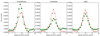 |
Fig. 14. Lyα (red dots) and UV (green squares) profiles in the spatial direction for the LAEVs in the identified overdensities (left), in the transition (middle) and field (rightpanel) regions. The curves represent Gaussian fits to the data. |
6.3. Simulating the Lyα profile of the VANDELS Lyα-emitting galaxies
To test if the HI column density and other galaxy properties can produce the Lyα profile we observe for the LAEVs in overdense regions, we make use of the public version of FLaREON (Gurung-López et al. 2019b), which is based on LyaRT (Orsi et al. 2012), a radiative transfer Monte Carlo code of Lyα emission. FLaREON predicts the Lyα line profile escaping a galaxy through different outflow configurations. Several outflow geometries are implemented in FLaREON, such as the commonly used thin shell of HI gas (Verhamme et al. 2006; Gronke & Dijkstra 2016), and a galactic wind (Fig. 1 in Gurung-López et al. 2019a). Additionally, the escaping line profile depends on the input dust reddening, the Vexp, and the HI column density. The characteristics of the Lyα line profile are strongly coupled with the properties of the outflow. To take into account the diversity of line profiles, we consider different outflow configurations. In particular, we run FLaREON with the following Vexp, NHI combinations: (i) 10 km sec−1, 1018 atoms cm−2, (ii) 10 km sec−1, 1021 atoms cm−2, (iii) 200 km sec−1, 1018 atoms cm−2, and (iv) 200 km sec−1, 1021 atoms cm−2. This choice of parameters englobes the lowest and highest values of Vexp and NHI, provided by FLaREON. Meanwhile, we fix the dust reddening to the median Av value of the nine LAEVs in overdense regions and of the 100 LAEVs in the field.
The Lyα line profile at high redshift is also affected by the presence of neutral hydrogen in the intergalactic medium (Laursen et al. 2011). In Gurung-López et al. (2020), the authors develop a method to compute the IGM impact on the Lyα emission in cosmological volumes. Their work is based on the state-of-the-art N-body simulation P-Millennium (Baugh et al. 2018) and the semi-analytic model of galaxy formation and evolution GALFORM (Lacey et al. 2016). The IGM absorption is computed taking into account the local density, velocity, and ionisation state of the IGM. Then, for every position in the simulation, an IGM transmission curve is computed integrating the IGM absorptions along a set of lines of sight. The authors found that, depending on the local density, the IGM transmission changes. In particular, denser regions exhibit higher absorption of the Lyα profile. Therefore, in order to take into account the presence of a dense environment, we convolve the Lyα line profiles produced by FLaREON with the median IGM transmission curve of the top 50% dense environments at z = 3.0 (resembling our identified overdensities) computed in the P-Millennium+GALFORM simulation.
In Fig. 15, we show the Lyα line profiles obtained with FLaREON. Models with Vexp > 150 km sec−1 and NHI< 1020 atoms cm−2 present a negligible blue peak and a dominant red peak with complicated structures on the red-side wing of the red peak (see for example the magenta curves in the left and middle panels of the figure) that would blend into a broad profile at our resolution. The resulting profile would appear as the one we observe for the stack of the field LAEVs. However, we want to investigate if there is any reasonable combination of parameters that reproduces a blue peak (in addition to a dominant red peak) as it can be seen in the stack profile of the LAEVs in overdense regions.
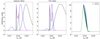 |
Fig. 15. Predicted Lyα profiles obtained with the FLaREON model. We present profiles obtained assuming the geometry of a galactic wind (left) and of a thin shell (middle), the typical dust reddening of the LAEVs in our identified overdensities, and considering the median IGM transmission curve of the top 50% dense environments at z = 3.0, as explained in the text. The model curves are arbitrarily normalized to the height of the stacked Lyα profile of LAEVs in our identified overdensities (Fig. 12). The different curves represent the following combinations of parameters, Vexp = 10 km sec−1, log(NHI) = 18 (green); Vexp = 10 km sec−1, log(NHI) = 21.3 (blue); Vexp = 200 km sec−1, log(NHI) = 18 (magenta); Vexp = 200 km sec−1, log(NHI) = 21.3 (black) for the galactic wind geometry; Vexp = 10 km sec−1, log(NHI) = 18 (green); Vexp = 10 km sec−1, log(NHI) = 21.5 (blue); Vexp = 200 km sec−1, log(NHI) = 18 (magenta); Vexp = 200 km sec−1, log(NHI) = 21.5 (black) for the thin shell geometry. The rightpanel shows models obtained assuming Vexp = 160, 170, 180, 190, 200 km sec−1 and log(NHI) = 19, where the widest profile corresponds to highest velocity for the geometry of a galactic wind (blue) and of a thin shell (green). The curves are arbitrarily normalized to the height of the stacked Lyα profile of LAEVs in the field. |
Inspecting the predicted line profiles, we find that the profiles with large Vexp and high NHICGM result in a main peak more redshifted and blue-to-red peak separations larger than what we observe in our spectra. Models with low expansion velocities, Vexp ∼ 10 km sec−1, and HI column densities of the order of log(NHICGM)∼21 produce Lyα lines with a visible blue peak, especially after applying the IGM transmission typical of overdense regions. As it is shown in Fig. 4 of Gurung-López et al. (2019b), HI column densities larger than 1020 atoms cm−2 could result in blue vs red peak separations even as large as 4 Å, as we observed in our data. In fact, we find that in the case of thin-shell and galactic-wind geometries a blue peak at a separation of about 4 Å from the red peak can be predicted when Vexp ∼ 10 km sec−1 and log(NHICGM) > 21 (see also Fig. 7e in Laursen et al. 2011).
Due to the low statistics, we just perform a qualitative comparison with FLaREON. According to this comparison, the stacked Lyα line profile of the LAEVs in overdense regions presented in this work is unlikely to be consistent with a model obtained from a galaxy with large-Vexp outflows and low HI column densities. The low Vexp, instead, can be related to the fact that the galaxies in overdense regions are currently forming stars at a low rate, preventing the formation of strong or fast outflows. The NHI could be high because we are studying regions of the Universe which are dense in terms of number density of galaxies and so maybe also dense of HI gas. It is also possible that the HI gas is trapped in the overdensity gravitational potential and stays in the medium surrounding the galaxies (e.g., Zheng et al. 2016). In addition to this, a large NHI could be characteristic of high mass galaxies which are experiencing quiescent star formation, as opposed to bursty phases maybe more typical of low mass LAEVs in the field. In fact, the FLaREON profiles with Vexp > 150 km sec−1 and NHI < 1020 atoms cm−2 qualitatively reproduce the Lyα stack of the LAEVs in the field. Even if a bigger sample of LAEVs in overdense regions would be desirable, we find evidence that the Lyα line shape is modulated by the surrounding environment.
7. Conclusions
With the aim of investigating whether Lyα-emitting galaxies trace the environment and its properties, we studied local densities in the CDFS and in the UDS. We made use of the VANDELS photometric catalog. The incompleteness of the catalog does not affect in a severe way the estimation of the local densities and the identification of overdense regions in our fields. Photometric redshift uncertainties are the main limit in the study of the environment, as we tested with mocks.
We identified and characterized 22 overdensities at 2 < z < 4 (Sect. 5). Some of these overdense regions show one main density peak, but the majority are composed of more than one structure. None of the identified overdensities seems to show properties similar to the virialized structures at z < 2, but we see that in some of them the members have rest-frame U − V colors redder than the field galaxies. Also, the identified overdensities are typically on the track of the evolution from protoclusters to Fornax-type cluster at z = 0.
Some of the overdensities occupy a large area of the field and may present more than one dense peak that are unlikely to be connected and to evolve in a unique structure at lower redshift. A test with mocks showed that some of the detected overdensities can be composed by more than one bound structure found in a N-body simulation, even when the positions of the galaxies are not affected by photometric redshift uncertainties. In an upcoming paper, we will study each overdensity and its fate to lower redshift in more detail. However, defining regions with high and low density in the VANDELS field is enough in this work to study the location of the Lyα-emitting galaxies with respect to the environment.
We studied the physical and spectroscopic properties of the Lyα-emitting galaxies detected in the first two seasons of the VANDELS survey. These LAEVs are VANDELS targets, drop-out galaxies by selection, and their location was not preselected in terms of density or environment. In the CDFS and in the UDS, we considered 51 and 80 galaxies, respectively, at 3 < zspec < 4 with 1< EW(Lyα) < 200 Å. In comparison to typical narrow-band selected LAEs, the LAEVs have lower sSFRs and are more massive, but have physical properties in agreement with models of Lyα-emitting galaxies (e.g., Gurung-López et al. 2020).
Among the selected LAEVs, only nine are members of the detected overdensities and 100 are located in the field. A KS test showed that we can not reject the null hypothesis that the EW(Lyα) (Fig. 9) and L(Lyα) (Fig. 11) of the LAEVs in the overdensities and in the field are drawn from the same distribution, but that we can reject the null hypothesis for their stellar masses, sSFRs, and rest-frame UV magnitudes (Fig. 10). We do not typically find the LAEVs in the cores of the most dense regions of the environment. However, the LAEVs in the identified overdensities tend to show higher stellar masses and lower sSFRs with respect to the ones in the field, but are brighter in the rest-frame UV and NIR, and some of them have a clear signature of dust content. Moreover, the LAEVs in overdensities share some physical properties of the galaxies without Lyα in emission in overdense regions.
We stacked the 1D Lyα profiles of the LAEVs in the detected overdensities and in the field (Fig. 12). The stack of the LAEVs in overdense regions shows a hint of a blue peak and that the Lyα emission is spatially more extended than the UV continuum.
We discussed the possible interpretation of the Lyα profiles in terms of the FLaREON model. Geometrical combinations of interstellar media with low expansion velocities and high HI column densities seem favourable to interpret the stack of the Lyα profiles of the LAEVs in our identified overdensities. Models with Vexp > 150 km sec−1 and NHI < 1020 atoms cm−2, at the resolution of our data, result in a broad red peak that qualitatively reproduce the Lyα stack of the LAEVs in the field. An outflow with low expansion velocity could be related to the low rate at which the galaxies are currently forming stars in overdense regions.
Guaita et al. (2017) found that Lyα emitters characterized by expansion velocities of the order of 300 km sec−1 and Lyα spatial extension comparable to that of the UV continuum could be experiencing bursty and short phases of star formation which tend to consume the HI gas quickly, preventing an efficient HI scattering and the formation of extended Lyα nebulae. On the other hand, the galaxies with interstellar media consistent with being static and HI column densities of the order 1021 atoms cm−2 could be characterized by longer phases of star formation which consume the HI gas slowly and can be characterized by extended Lyα nebulae.
In the overdensities we study here, galaxies in general and LAEVs in particular could be experiencing either long or slow phases of star formation as opposed to short bursty phases due to the effects of environment. Despite the low statistics, thanks to the information provided by the Lyα emission, Lyα emitters may provide useful insights on the environment in which they reside.
This name is a simplification since we do not know for sure the fate of a protocluster and if it will really evolve into a cluster.
Grazian et al. (2006), Vanzella et al. (2008, 2009), Wuyts et al. (2008, 2009), Rhoads et al. (2009), Straughn et al. (2009), Balestra et al. (2010), Cooper et al. (2012), Kurk et al. (2013), Le Fèvre et al. (2013, 2015), Trump et al. (2013), Kriek et al. (2015), Morris et al. (2015), Momcheva et al. (2016).
Rmeandist is always lower than 2.5 cMpc/2 to avoid overlaps between the overdensity and the field volumes.
Acknowledgments
We thank the ESO staff for their continuous support for the VANDELS survey, particularly the Paranal staff, who helped us to conduct the observations, and the ESO user support group in Garching. We thank Manuel Aravena, Jeremy Blazoit, Thibault Garel, Sam Kim, Roberto Gonzalez for useful discussions, Alvaro Orsi and Siddharta Gurung-Lopez for providing radiative transfer models. We thank the ESO scientific visitor program during which part of this project was carried on. We acknowledge support from CONICYT grants Basal-CATA Basal AFB-170002 (LG, FEB), and Programa de Astronomia FONDO ALMA 2016 31160033 (LG), and the Ministry of Economy, Development, and Tourism’s Millennium Science Initiative through grant IC120009, awarded to The Millennium Institute of Astrophysics, MAS (FEB). RA acknowledges support from FONDECYT Regular Grant 1202007.
References
- Abell, G. O. 1958, ApJS, 3, 211 [NASA ADS] [CrossRef] [Google Scholar]
- Andreon, S., Newman, A. B., Trinchieri, G., et al. 2014, A&A, 565, A120 [NASA ADS] [CrossRef] [EDP Sciences] [Google Scholar]
- Balestra, I., Mainieri, V., Popesso, P., et al. 2010, A&A, 512, A12 [NASA ADS] [CrossRef] [EDP Sciences] [Google Scholar]
- Baugh, C. M., Gonzalez-Perez, V., del P Lagos, C., et al. 2018, MNRAS, [Google Scholar]
- Baugh, C. M., Gonzalez-Perez, V., Lagos, C. d. P., et al. 2019, MNRAS, 483, 4922 [NASA ADS] [CrossRef] [Google Scholar]
- Beers, T. C., Flynn, K., & Gebhardt, K. 1990, AJ, 100, 32 [NASA ADS] [CrossRef] [Google Scholar]
- Bertin, E., & Arnouts, S. 1996, A&AS, 117, 393 [NASA ADS] [CrossRef] [EDP Sciences] [Google Scholar]
- Bruzual, G., & Charlot, S. 2003, MNRAS, 344, 1000 [NASA ADS] [CrossRef] [Google Scholar]
- Calzetti, D., Armus, L., Bohlin, R. C., et al. 2000, ApJ, 533, 682 [NASA ADS] [CrossRef] [Google Scholar]
- Carnall, A. C., McLure, R. J., Dunlop, J. S., et al. 2019, MNRAS, 490, 417 [Google Scholar]
- Castellano, M., Salimbeni, S., Trevese, D., et al. 2007, ApJ, 671, 1497 [Google Scholar]
- Chiang, Y.-K., Overzier, R., & Gebhardt, K. 2013, ApJ, 779, 127 [NASA ADS] [CrossRef] [Google Scholar]
- Contini, E., De Lucia, G., Hatch, N., Borgani, S., & Kang, X. 2016, MNRAS, 456, 1924 [NASA ADS] [CrossRef] [Google Scholar]
- Cooper, M. C., Yan, R., Dickinson, M., et al. 2012, MNRAS, 425, 2116 [NASA ADS] [CrossRef] [Google Scholar]
- Cortese, L., Gavazzi, G., Boselli, A., et al. 2006, A&A, 453, 847 [Google Scholar]
- Cucciati, O., Zamorani, G., Lemaux, B. C., et al. 2014, A&A, 570, A16 [NASA ADS] [CrossRef] [EDP Sciences] [Google Scholar]
- Cucciati, O., Lemaux, B. C., Zamorani, G., et al. 2018, A&A, 619, A49 [NASA ADS] [CrossRef] [EDP Sciences] [Google Scholar]
- Curtis-Lake, E., McLure, R. J., Pearce, H. J., et al. 2012, MNRAS, 422, 1425 [NASA ADS] [CrossRef] [EDP Sciences] [Google Scholar]
- Davis, M., Efstathiou, G., Frenk, C. S., & White, S. D. M. 1985, ApJ, 292, 371 [NASA ADS] [CrossRef] [Google Scholar]
- De Lucia, G., & Blaizot, J. 2007, MNRAS, 375, 2 [NASA ADS] [CrossRef] [Google Scholar]
- Durkalec, A., Le Fèvre, O., Pollo, A., et al. 2015, A&A, 583, A128 [Google Scholar]
- Forrest, B., Tran, K.-V. H., Broussard, A., et al. 2017, ApJ, 838, L12 [NASA ADS] [CrossRef] [Google Scholar]
- Franck, J. R., & McGaugh, S. S. 2016, ApJ, 833, 15 [NASA ADS] [CrossRef] [Google Scholar]
- Fukugita, M., Shimasaku, K., & Ichikawa, T. 1995, PASP, 107, 945 [NASA ADS] [CrossRef] [Google Scholar]
- Galametz, A., Grazian, A., Fontana, A., et al. 2013, ApJS, 206, 10 [NASA ADS] [CrossRef] [Google Scholar]
- Garel, T., Blaizot, J., Guiderdoni, B., et al. 2015, MNRAS, 450, 1279 [Google Scholar]
- Garilli, B., Fumana, M., Franzetti, P., et al. 2010, PASP, 122, 827 [NASA ADS] [CrossRef] [Google Scholar]
- Gehrels, N. 1986, ApJ, 303, 336 [NASA ADS] [CrossRef] [Google Scholar]
- Gladders, M. D., & Yee, H. K. C. 2000, in Cosmic Evolution and Galaxy Formation: Structure, Interactions, and Feedback, eds. J. Franco, L. Terlevich, O. López-Cruz, & I. Aretxaga, ASP Conf. Ser., 215, 233 [Google Scholar]
- Grazian, A., Fontana, A., de Santis, C., et al. 2006, A&A, 449, 951 [NASA ADS] [CrossRef] [EDP Sciences] [Google Scholar]
- Grogin, N. A., Kocevski, D. D., Faber, S. M., et al. 2011, ApJS, 197, 35 [NASA ADS] [CrossRef] [Google Scholar]
- Gronke, M., & Dijkstra, M. 2016, ApJ, 826, 14 [NASA ADS] [CrossRef] [Google Scholar]
- Gronwall, C., Ciardullo, R., Hickey, T., et al. 2007, ApJ, 667, 79 [NASA ADS] [CrossRef] [Google Scholar]
- Guaita, L., Gawiser, E., Padilla, N., et al. 2010, ApJ, 714, 255 [NASA ADS] [CrossRef] [Google Scholar]
- Guaita, L., Talia, M., Pentericci, L., et al. 2017, A&A, 606, A19 [NASA ADS] [CrossRef] [EDP Sciences] [Google Scholar]
- Guo, Y., Ferguson, H. C., Giavalisco, M., et al. 2013, ApJS, 207, 24 [NASA ADS] [CrossRef] [Google Scholar]
- Gurung-López, S., Orsi, Á. A., & Bonoli, S. 2019a, MNRAS, 490, 733 [NASA ADS] [CrossRef] [Google Scholar]
- Gurung-López, S., Orsi, Á. A., Bonoli, S., Baugh, C. M., & Lacey, C. G. 2019b, MNRAS, 486, 1882 [NASA ADS] [CrossRef] [Google Scholar]
- Gurung-López, S., Orsi, Á. A., Bonoli, S., et al. 2020, MNRAS, 491, 3266 [Google Scholar]
- Hagen, A., Zeimann, G. R., Behrens, C., et al. 2016, ApJ, 817, 79 [NASA ADS] [CrossRef] [EDP Sciences] [Google Scholar]
- Haines, C. P., Pereira, M. J., Smith, G. P., et al. 2015, ApJ, 806, 101 [NASA ADS] [CrossRef] [Google Scholar]
- Hatch, N. A., Kurk, J. D., Pentericci, L., et al. 2011, MNRAS, 415, 2993 [NASA ADS] [CrossRef] [Google Scholar]
- Hirschmann, M., De Lucia, G., & Fontanot, F. 2016, MNRAS, 461, 1760 [NASA ADS] [CrossRef] [Google Scholar]
- Kang, E., & Im, M. 2015, J. Korean Astron. Soc., 48, 21 [Google Scholar]
- Kodama, T., Tanaka, I., Kajisawa, M., et al. 2007, MNRAS, 377, 1717 [NASA ADS] [CrossRef] [Google Scholar]
- Koekemoer, A. M., Faber, S. M., Ferguson, H. C., et al. 2011, ApJS, 197, 36 [NASA ADS] [CrossRef] [Google Scholar]
- Koyama, Y., Kodama, T., Tadaki, K.-I., et al. 2013, MNRAS, 428, 1551 [CrossRef] [Google Scholar]
- Kriek, M., Shapley, A. E., Reddy, N. A., et al. 2015, ApJS, 218, 15 [NASA ADS] [CrossRef] [Google Scholar]
- Kubo, M., Uchimoto, Y. K., Yamada, T., et al. 2013, ApJ, 778, 170 [NASA ADS] [CrossRef] [Google Scholar]
- Kurk, J., Cimatti, A., Daddi, E., et al. 2013, A&A, 549, A63 [NASA ADS] [CrossRef] [EDP Sciences] [Google Scholar]
- Lacey, C. G., Baugh, C. M., Frenk, C. S., et al. 2016, MNRAS, 462, 3854 [NASA ADS] [CrossRef] [Google Scholar]
- Laursen, P., Sommer-Larsen, J., & Razoumov, A. O. 2011, ApJ, 728, 52 [NASA ADS] [CrossRef] [Google Scholar]
- Le Fèvre, O., Cassata, P., Cucciati, O., et al. 2013, A&A, 559, A14 [NASA ADS] [CrossRef] [EDP Sciences] [Google Scholar]
- Le Fèvre, O., Tasca, L. A. M., Cassata, P., et al. 2015, A&A, 576, A79 [NASA ADS] [CrossRef] [EDP Sciences] [Google Scholar]
- Lemaux, B. C., Cucciati, O., Tasca, L. A. M., et al. 2014, A&A, 572, A41 [NASA ADS] [CrossRef] [EDP Sciences] [Google Scholar]
- Lemaux, B. C., Le Fèvre, O., Cucciati, O., et al. 2018, A&A, 615, A77 [NASA ADS] [CrossRef] [EDP Sciences] [Google Scholar]
- Lenz, D. D., & Ayres, T. R. 1992, PASP, 104, 1104 [NASA ADS] [CrossRef] [Google Scholar]
- Madau, P. 1995, ApJ, 441, 18 [NASA ADS] [CrossRef] [Google Scholar]
- Maltby, D. T., Almaini, O., Wild, V., et al. 2016, MNRAS, 459, L114 [Google Scholar]
- Marchi, F., Pentericci, L., Guaita, L., et al. 2019, A&A, 631, A19 [NASA ADS] [CrossRef] [EDP Sciences] [Google Scholar]
- McLure, R. J., Pentericci, L., Cimatti, A., et al. 2018, MNRAS, [Google Scholar]
- Miller, T. B., Chapman, S. C., Aravena, M., et al. 2018, Nature, 556, 469 [NASA ADS] [CrossRef] [Google Scholar]
- Momcheva, I. G., Brammer, G. B., van Dokkum, P. G., et al. 2016, ApJS, 225, 27 [NASA ADS] [CrossRef] [Google Scholar]
- Morris, A. M., Kocevski, D. D., Trump, J. R., et al. 2015, AJ, 149, 178 [NASA ADS] [CrossRef] [Google Scholar]
- Muldrew, S. I., Hatch, N. A., & Cooke, E. A. 2015, MNRAS, 452, 2528 [NASA ADS] [CrossRef] [Google Scholar]
- Newman, A. B., Ellis, R. S., Andreon, S., et al. 2014, ApJ, 788, 51 [NASA ADS] [CrossRef] [Google Scholar]
- Orsi, A., Lacey, C. G., & Baugh, C. M. 2012, MNRAS, 425, 87 [NASA ADS] [CrossRef] [Google Scholar]
- Overzier, R. A. 2016, A&ARv, 24, 14 [NASA ADS] [CrossRef] [Google Scholar]
- Pentericci, L., Kurk, J. D., Röttgering, H. J. A., et al. 2000, A&A, 361, L25 [NASA ADS] [Google Scholar]
- Pentericci, L., Castellano, M., Menci, N., et al. 2013, A&A, 552, A111 [Google Scholar]
- Pentericci, L., McLure, R. J., Franzetti, P., Garilli, B., & the VANDELS team 2018a, ArXiv e-prints [arXiv:1811.05298] [Google Scholar]
- Pentericci, L., McLure, R. J., Garilli, B., et al. 2018b, A&A, 616, A174 [NASA ADS] [CrossRef] [EDP Sciences] [Google Scholar]
- Press, W. H., & Davis, M. 1982, ApJ, 259, 449 [NASA ADS] [CrossRef] [Google Scholar]
- Rhoads, J. E., Malhotra, S., Pirzkal, N., et al. 2009, ApJ, 697, 942 [Google Scholar]
- Salimbeni, S., Giallongo, E., Menci, N., et al. 2008, A&A, 477, 763 [NASA ADS] [CrossRef] [EDP Sciences] [Google Scholar]
- Salimbeni, S., Castellano, M., Pentericci, L., et al. 2009, A&A, 501, 865 [NASA ADS] [CrossRef] [EDP Sciences] [Google Scholar]
- Santini, P., Ferguson, H. C., Fontana, A., et al. 2015, ApJ, 801, 97 [NASA ADS] [CrossRef] [Google Scholar]
- Shimakawa, R., Kodama, T., Tadaki, K.-I., et al. 2015, MNRAS, 448, 666 [NASA ADS] [CrossRef] [Google Scholar]
- Springel, V., White, S. D. M., Jenkins, A., et al. 2005, Nature, 435, 629 [NASA ADS] [CrossRef] [PubMed] [Google Scholar]
- Steidel, C. C., Adelberger, K. L., Dickinson, M., et al. 1998, ApJ, 492, 428 [Google Scholar]
- Steidel, C. C., Adelberger, K. L., Shapley, A. E., et al. 2005, ApJ, 626, 44 [NASA ADS] [CrossRef] [Google Scholar]
- Stott, J. P., Hickox, R. C., Edge, A. C., et al. 2012, MNRAS, 422, 2213 [NASA ADS] [CrossRef] [Google Scholar]
- Straughn, A. N., Pirzkal, N., Meurer, G. R., et al. 2009, AJ, 138, 1022 [Google Scholar]
- Strazzullo, V., Gobat, R., Daddi, E., et al. 2013, ApJ, 772, 118 [NASA ADS] [CrossRef] [Google Scholar]
- Strazzullo, V., Daddi, E., Gobat, R., et al. 2016, ApJ, 833, L20 [NASA ADS] [CrossRef] [Google Scholar]
- Trevese, D., Castellano, M., Fontana, A., & Giallongo, E. 2007, A&A, 463, 853 [NASA ADS] [CrossRef] [EDP Sciences] [Google Scholar]
- Trump, J. R., Konidaris, N. P., Barro, G., et al. 2013, ApJ, 763, L6 [Google Scholar]
- van der Wel, A., Bell, E. F., Häussler, B., et al. 2012, ApJS, 203, 24 [NASA ADS] [CrossRef] [Google Scholar]
- Vanzella, E., Cristiani, S., Dickinson, M., et al. 2008, A&A, 478, 83 [NASA ADS] [CrossRef] [EDP Sciences] [Google Scholar]
- Vanzella, E., Giavalisco, M., Dickinson, M., et al. 2009, ApJ, 695, 1163 [NASA ADS] [CrossRef] [Google Scholar]
- Venemans, B. P., Röttgering, H. J. A., Miley, G. K., et al. 2007, A&A, 461, 823 [NASA ADS] [CrossRef] [EDP Sciences] [Google Scholar]
- Verhamme, A., Schaerer, D., & Maselli, A. 2006, A&A, 460, 397 [NASA ADS] [CrossRef] [EDP Sciences] [Google Scholar]
- Verhamme, A., Orlitová, I., Schaerer, D., & Hayes, M. 2015, A&A, 578, A7 [NASA ADS] [CrossRef] [EDP Sciences] [Google Scholar]
- Verhamme, A., Orlitová, I., Schaerer, D., et al. 2017, A&A, 597, A13 [NASA ADS] [CrossRef] [EDP Sciences] [Google Scholar]
- Wainer, H., & Thissen, D. 1976, Psychometrika, 41, 9 [CrossRef] [Google Scholar]
- Willis, J. P., Clerc, N., Bremer, M. N., et al. 2013, MNRAS, 430, 134 [NASA ADS] [CrossRef] [Google Scholar]
- Wuyts, S., Labbé, I., Förster Schreiber, N. M., et al. 2008, ApJ, 682, 985 [NASA ADS] [CrossRef] [Google Scholar]
- Wuyts, S., van Dokkum, P. G., Franx, M., et al. 2009, ApJ, 706, 885 [NASA ADS] [CrossRef] [Google Scholar]
- Zabludoff, A. I., Geller, M. J., Huchra, J. P., & Vogeley, M. S. 1993, AJ, 106, 1273 [NASA ADS] [CrossRef] [Google Scholar]
- Zheng, Z.-Y., Malhotra, S., Rhoads, J. E., et al. 2016, ApJS, 226, 23 [NASA ADS] [CrossRef] [Google Scholar]
- Zirm, A. W., Toft, S., & Tanaka, M. 2012, ApJ, 744, 181 [Google Scholar]
- Zoldan, A., De Lucia, G., Xie, L., Fontanot, F., & Hirschmann, M. 2017, MNRAS, 465, 2236 [Google Scholar]
Appendix A: Location of the overdensities identified in the CDFS and in the UDS
We present here the position of the identified overdensities in space. We also show the position of the structures detected in the literature in the same areas.
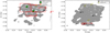 |
Fig. A.1. Density levels for galaxies at 2.25 < z < 2.35 (left) and 2.45 < z < 2.55 (right) in the CDFS. The contours represent 3, 2, 1, 0.5σ over the mean value of the local densities associated to the galaxies in the indicated redshift bin. Spectroscopic redshifts from VANDELS (VANDELS_notLAEspec) are indicated as black diamonds, VANDELS LAEs are indicated as red stars. For them, we also indicate the spectroscopic redshifts. Red rectangles represent the location of the identified overdensities. The center of these structures is shown with red triangles. The redshift of the highest-density peak and the redshift range of the structures is written in red. We also show the position of the center of structures detected in the literature in the same field and in the same redshift ranges, Salimbeni et al. (2009; green squares), Franck & McGaugh (2016; big red triangles), Kang & Im (2015; yellow stars). We write the redshifts of the literature-structure cores in green, red, and yellow, respectively. |
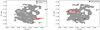 |
Fig. A.2. Density levels for galaxies at 2.65 < z < 2.75 (left) and 2.75 < z < 2.85 (right) in the CDFS. |
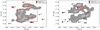 |
Fig. A.3. Density levels for galaxies at 3.15 < z < 3.25 (left) and 3.25 < z < 3.35 (right) in the CDFS. |
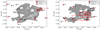 |
Fig. A.4. Density levels for galaxies at 3.35 < z < 3.45 (left) and 3.45 < z < 3.55 (right) in the CDFS. |
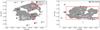 |
Fig. A.5. Density levels for galaxies at 3.65 < z < 3.75 (left) in the CDFS and 2.25 < z < 2.35 (right) in the UDS. |
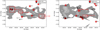 |
Fig. A.6. Density levels for galaxies at 3.25 < z < 3.35 (left) and 3.45 < z < 3.55 (right) in the UDS. |
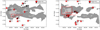 |
Fig. A.7. Density levels for galaxies at 3.55 < z < 3.65 (left) and 3.65 < z < 3.75 (right) in the UDS. |
Appendix B: 3D visualization of the overdensities identified in the CDFS and in the UDS
In this section, we show the 3D visualization of the identified overdensities. It is worth noting that the redshift direction can comprise much larger physical sizes than the RA and declination. This is a result of the way our code detects overdensities. In fact, to calculate local densities, we choose an initial cell size in the redshift direction proportional to the photometric redshift uncertainty, the largest uncertainty we have. The extension of each cell is characterized by a parallelepiped volume, elongated towards the redshift direction (as described in Sect. 3). Within the detected overdensities, there exist dense cores, compact also in the redshift direction, that could evolve in protoclusters.
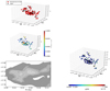 |
Fig. B.1. 3D visualization of the overdensity identified at z = 2.29 in the CDFS. In the firstpanel, we show the overdensity members in the RA,dec,redshift space in red. The members with spectroscopic redshifts either from VANDELS or from the literature are shown in black with the black numbers indicating the zspec. In the secondpanel, the color coding is the density associated to each member with respect to density associated to the highest-density peak. The thirdpanel shows the density map in 2D. The contours represent 3, 2, 1, 0.5σ over the mean value of the local densities associated to the galaxies in the redshift range, zpeak − 0.05 < z < zpeak + 0.05, where zpeak is the redshift of the highest-density peak and it is shown for reference. The fourthpanel is as the first one, but the color coding of the symbols refers to the sSFR. The horizontal color-bar label shows the minimum, the mean, and the maximum value of sSFR. |
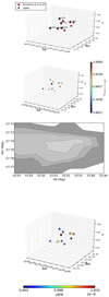 |
Fig. B.10. Same as Fig. B.1 for the overdensity detected at z = 3.43 in the CDFS. |
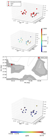 |
Fig. B.11. Same as Fig. B.1 for the overdensity detected at z = 3.54 in the CDFS. |
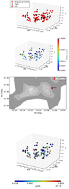 |
Fig. B.12. Same as Fig. B.1 for the overdensity detected at z = 3.55 in the CDFS. |
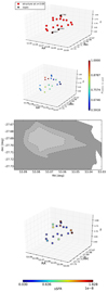 |
Fig. B.13. Same as Fig. B.1 for the overdensity detected at z = 3.69 in the CDFS. |
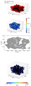 |
Fig. B.14. Same as Fig. B.1 for the overdensity detected at z = 2.33 in the UDS. |
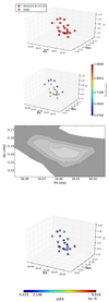 |
Fig. B.15. Same as Fig. B.1 for the overdensity detected at z = 3.25 in the UDS. |
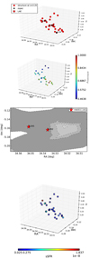 |
Fig. B.16. Same as Fig. B.1 for the overdensity detected at z = 3.25 in the UDS. |
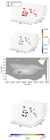 |
Fig. B.17. Same as Fig. B.1 for the overdensity detected at z = 3.27 in the UDS. |
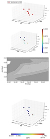 |
Fig. B.18. Same as Fig. B.1 for the overdensity detected at z = 3.49 in the UDS. |
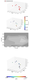 |
Fig. B.19. Same as Fig. B.1 for the overdensity detected at z = 3.51 in the UDS. |
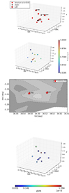 |
Fig. B.20. Same as Fig. B.1 for the overdensity detected at z = 3.65 in the UDS. |
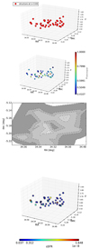 |
Fig. B.21. Same as Fig. B.1 for the overdensity detected at z = 3.69 in the UDS. |
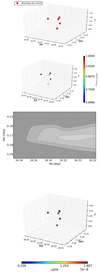 |
Fig. B.22. Same as Fig. B.1 for the overdensity detected at z = 4.01 in the UDS. |
Appendix C: Color, magnitude, stellar mass, and specific star-formation rate versus environment
For the overdensities discussed in Sect. 5.2, we present here stellar mass (upper left), sSFR (upper right), rest-frame U − V color (lower right) versus the density to highest-density peak, and rest-frame U − V color versus rest-frame V magnitude for the overdensity members (big red dots) and field galaxies (small black dots). The overdensity members with spectroscopic redshifts either from VANDELS or from the literature are shown as big black dots. The stars indicate the properties of the LAEVs in the overdensities described in Sect. 7. We show KS statistics for the distributions of stellar masses, sSFRs, and rest-frame U − V colors of the overdensity members and field galaxies as KS and p parameters. The red horizontal lines in the lower right panels indicate the position of the red sequence and its uncertainty according to the definition of Willis et al. (2013).
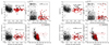 |
Fig. C.1. As described in the text of this section for the overdensities detected at z = 2.29 (leftpanels) and z = 2.30 (rightpanels) in the CDFS. |
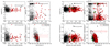 |
Fig. C.2. As described in the text of this section for the overdensities detected at z = 2.80 (leftpanels) and z = 3.17 (rightpanels) in the CDFS. |
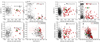 |
Fig. C.3. As described in the text of this section for the overdensities detected at z = 3.54 (leftpanels) and z = 3.55 (rightpanels) in the CDFS. |
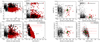 |
Fig. C.4. As described in the text of this section for the overdensities detected at z = 2.33 (leftpanels) and z = 3.25 (rightpanels) in the UDS. |
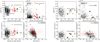 |
Fig. C.5. As described in the text of this section for the overdensities detected at z = 3.27 (leftpanels) and z = 3.65 (rightpanels) in the UDS. |
Appendix D: Color-color diagram versus environment and galaxy shape
For the overdensities discussed in Sect. 5, we present here rest-frame U − V colors as a function of rest-frame V − J colors for the overdensity members (red dots) and field galaxies (small black dots) (upper left), for the overdensity members and color coded according to the sSFR (upper right), for the overdensity members and color coded according to the Sersic index obtained with GALFIT (lower left), for the overdensity members and color coded according to the GALFIT fit axis ratio (lower right). The morphological parameters come from the analysis described in van der Wel et al. (2012). The ticks in the vertical color bars indicate the maximum, the average, and the minimum value of labelled quantity. Generally, the members with higher rest-frame U − V colors are characterized by sSFR values lower than the mean value among the members.
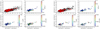 |
Fig. D.1. As described in the text of this section for the overdensities detected at z = 2.29 (leftpanels) and z = 2.30 (rightpanels) in the CDFS. |
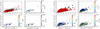 |
Fig. D.2. As described in the text of this section for the overdensities detected at z = 2.80 (leftpanels) and z = 3.17 (rightpanels) in the CDFS. |
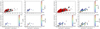 |
Fig. D.3. As described in the text of this section for the overdensities detected at z = 3.54 (leftpanels) and z = 3.55 (rightpanels) in the CDFS. |
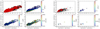 |
Fig. D.4. As described in the text of this section for the overdensities detected at z = 2.33 (leftpanels) and z = 3.25 (rightpanels) in the UDS. |
 |
Fig. D.5. As described in the text of this section for the overdensities detected at z = 3.27 (leftpanels) and z = 3.65 (rightpanels) in the UDS. |
All Tables
All Figures
|
Fig. 1. Redshift distribution of the sources in the input catalog of the CDFS (left panel) and of the UDS (right panel). The red histograms represent the sources with photometric and spectroscopic redshifts, the green histograms the sources with spectroscopic redshifts from the literature. The inserts show the redshift distributions of the Lyα-emitting galaxies selected from the VANDELS database and used in this work. |
| In the text | |
|
Fig. 2. Magnitude distribution of sources with photometric (upper left), spectroscopic redshifts from the literature (upper right), from VANDELS (lower left), and of the Lyα-emitting galaxies selected from the VANDELS database (lower right) in the CDFS (weak line) and in the UDS (strong line). |
| In the text | |
|
Fig. 3. Mean local density versus redshift for the CDFS (upper panel) and for the UDS (lower panel) shown as dashed solid curves. The mean corresponds to the average of the local density values in each bins of Δz = 0.02, after the application of sigma clipping, as explained in the text. Vertical solid lines represent the redshifts of the detected overdensities. In the lower panel, vertical dashed lines correspond to two slightly lower-threshold overdensities at z ∼ 2.8 (THRESHOLD = 4 instead of 6). |
| In the text | |
|
Fig. 4. Properties of the overdensities detected among the mock galaxies with isel ≤ 27.5 at 2 < z < 3 (red) and 3 < z < 4 (blue). The properties of the fiducial run overdensities (2 < z < 3FID and 3 < z < 4FID) are shown as dots and the properties of the overdensities detected after including zphot errors (mimicking the VANDELS data) and adopting THRESHOLD = 6 (2 < z < 3TH6 and 3 < z < 4TH6) are shown as stars. The leftpanels show the total number of members versus the mean distance between the members and the highest-density peak, the rightpanels show the maximum distance between the members and the highest-density peak and the standard deviation of the observed redshifts in velocity [c × stdev(zobs)]/[1 + mean(zobs)]. The fiducial-run overdensities missed after applying photometric uncertainties are indicated with black circles around the dots (missed). The ‘fake’ overdensities at z ∼ 3 (3 < z < 4TH6fake), not detected in the fiducial run, are shown as squares. To read this figure, we remind that each star (recovered overdensity) corresponds to a dot (fiducial-run overdensity) without black circle. The overdensities detected among the mock galaxies with isel ≤ 26.1 share the same properties of the ones detected among the mock galaxies with isel ≤ 27.5. |
| In the text | |
|
Fig. 5. Redshift distribution of the galaxies in the overdensities identified in the CDFS. The red histograms include both spectroscopic and photometric redshifts, while black histograms only the spectroscopic ones. The histogram bin is 0.02 in redshift. Some of overdensities are likely composed of more than one density peak. |
| In the text | |
|
Fig. 5. continued. |
| In the text | |
|
Fig. 6. Same as Fig. 5 for the overdensities identified in the UDS. Some of the overdensities could be composed of more than one density peak, such as the structure at z ≃ 2.33. |
| In the text | |
|
Fig. 7. Density map of two peculiar overdensities. The structures at z = 3.17 in the CDFS is shown in the leftpanel, the structures at z = 2.33 in the UDS is shown in the rightpanel. Red diamonds correspond to the spectroscopic members within the lowest redshift peaks, blue diamonds to the intermediate redshift peaks, green diamonds to the highest redshift peaks as seen in Fig. 6 and explained in the text. |
| In the text | |
|
Fig. 8. Leftpanel: mean rest-frame U − V color of the galaxies in the 22 overdensities identified at 2 < z < 4 versus redshift of their highest-density peaks (big black diamonds). We, also, show mean color and mean photometric redshift for star-forming galaxies (big magenta squares) and Lyman Break galaxies (big green circles) as classified in Pentericci et al. (2018a) and for the structures detected in the mocks, in the fiducial run (small gray circles) and in the run with parameters as in the real data (small black circles). Rightpanel: difference between the mean rest-frame U − V color of the overdensity members and the mean rest-frame U − V color of field galaxies versus the mean rest-frame U − V color of the overdensity members. The color coding indicates the redshift of the highest-density peak of the identified overdensities, blue for z < 2.7, green for 2.7 ≤ z ≤ 3.3, and red for z > 3.3. The error bars correspond to the standard error of the means. As a reference, the rest-frame U − V color for a representative cluster at z = 0 is equal to 1.4 and that of field galaxies is 0.5. To derive these values, we assume that a z = 0 cluster contains a well defined red sequence with a dominance of E and S0 galaxies and that field galaxies are a blue population (Fukugita et al. 1995). |
| In the text | |
|
Fig. 9. Normalized Lyα equivalent width distribution of the Lyα-emitting galaxies selected from the VANDELS database (LAEVs). The dashed histogram corresponds to the entire sample of LAEVs. The thin black and red histograms are the distributions for the LAEVs located in the field and members of the detected overdensities (as explained in the text), respectively. |
| In the text | |
|
Fig. 10. Upper panels: LAEV physical properties with respect to the environment in the VANDELS fields. The LAEVs located in the identified overdensities and with EW(Lyα) > 20 Å are shown as red stars, the ones with EW(Lyα) < 20 Å are shown as green stars, the ones located in transition regions are shown as cyan circles and in the field as black circles. Dashed lines indicate the median values of sSFR, stellar mass, and EW(Lyα) = 20 Å of the entire LAEV sample. The physical properties we investigate are sSFR versus EW(Lyα) (upper left), stellar mass versus EW(Lyα) (upper right), dust reddening, Av, versus rest-frame optical magnitude (lower left), rest-frame NIR magnitude versus rest-frame UV magnitude (lower right). The squares with error bars represent the typical parameter uncertainties coming from the SED fitting (see the upcoming work on SED fitting parameters). Lower panels: median physical properties of the LAEVs and of all the galaxies in the input catalog located in overdensities (red symbols) and in the field (black symbols). The medians are presented as diamonds for all the galaxies in the input catalog and stars for the LAEVs. The error bars on the medians correspond to the uncertainties due to SED fitting. The physical properties we investigate are sSFR versus stellar mass (upper left), stellar mass versus distance to the highest-density peak (upper right) of the identified overdensities, dust reddening, Av, versus rest-frame optical magnitude (lower left), rest-frame NIR magnitude versus rest-frame UV magnitude (lower right). |
| In the text | |
|
Fig. 11. Upper panel: Lyα flux vs Lyα equivalent width. lower panel: Lyα luminosity vs Lyα equivalent width. Green (red) stars indicate LAEVs in the identified overdensities with EW(Lyα) < 20 Å (EW(Lyα) > 20 Å), black dots indicate the LAEVs in the field. The vertical lines correspond to the mean (solid) and median (dashed) values of the EW(Lyα) of LAEVs in overdensities (red) and in the field (black). The horizontal lines correspond to the mean (solid) and median (dashed) values of the F(Lyα) and L(Lyα) of the LAEVs in the detected overdensities (red) and in the field (black). The shaded areas indicate the standard deviation of the means. The mean and median values of the F(Lyα) of the LAEVs in the detected overdensities and the median value of the F(Lyα) of the LAEVs in the field overlap. The mean and median values of the L(Lyα) is 1.4 ± 0.4 × 1042 and 1.3 × 1042 erg sec−1 for the LAEVs in the detected overdensities, while they are 2.9 ± 0.5 × 1042 and 1.6 × 1042 erg sec−1 for the LAEVs in the field. The median value of the LAEVs in the identified overdensities with EW(Lyα) < 20 Å (> 20 Å) is 7.4 × 1041 erg sec−1 (1.7 × 1042 erg sec−1). |
| In the text | |
|
Fig. 12. Upper panels: stacks of the Lyα profiles of the LAEVs in the identified overdensities (leftpanel), transition (middlepanel), and field (rightpanel) regions. The green shaded areas indicate the standard deviation of the mean of the fluxes at each wavelength among all the LAEVs in a certain density category. The observed profiles of the LAEVs in overdensity (transition) (field) regions is shown in red (blue) (black) in every panel. The dashed-dotted lines show the median stacks. Lower panels: asymmetric Gaussian curves, best fits of the stacks (dots with errorbars) in the upper panels. In each panel, red is used for the LAEVs in the identified overdensities, blue for the LAEVs in transition regions, black for the LAEVs in the field. The best fits of the asymmetric Gaussian curves provide the following parameters (λ, FWHM, A) = (1215, 4 Å, 0.86), (1215, 3 Å, 0.95), and (1215, 3 Å, 0.83) for the left, middle, and right stack, respectively. |
| In the text | |
|
Fig. 13. Stacks of the 2D spectra of the LAEVs in the identified overdensities (upper), in the transition (middle), and field (lower panel) regions at the wavelength of Lyα (leftpanels) and of the UV continuum at 1400 Å (rightpanels) rest frame. |
| In the text | |
|
Fig. 14. Lyα (red dots) and UV (green squares) profiles in the spatial direction for the LAEVs in the identified overdensities (left), in the transition (middle) and field (rightpanel) regions. The curves represent Gaussian fits to the data. |
| In the text | |
|
Fig. 15. Predicted Lyα profiles obtained with the FLaREON model. We present profiles obtained assuming the geometry of a galactic wind (left) and of a thin shell (middle), the typical dust reddening of the LAEVs in our identified overdensities, and considering the median IGM transmission curve of the top 50% dense environments at z = 3.0, as explained in the text. The model curves are arbitrarily normalized to the height of the stacked Lyα profile of LAEVs in our identified overdensities (Fig. 12). The different curves represent the following combinations of parameters, Vexp = 10 km sec−1, log(NHI) = 18 (green); Vexp = 10 km sec−1, log(NHI) = 21.3 (blue); Vexp = 200 km sec−1, log(NHI) = 18 (magenta); Vexp = 200 km sec−1, log(NHI) = 21.3 (black) for the galactic wind geometry; Vexp = 10 km sec−1, log(NHI) = 18 (green); Vexp = 10 km sec−1, log(NHI) = 21.5 (blue); Vexp = 200 km sec−1, log(NHI) = 18 (magenta); Vexp = 200 km sec−1, log(NHI) = 21.5 (black) for the thin shell geometry. The rightpanel shows models obtained assuming Vexp = 160, 170, 180, 190, 200 km sec−1 and log(NHI) = 19, where the widest profile corresponds to highest velocity for the geometry of a galactic wind (blue) and of a thin shell (green). The curves are arbitrarily normalized to the height of the stacked Lyα profile of LAEVs in the field. |
| In the text | |
|
Fig. A.1. Density levels for galaxies at 2.25 < z < 2.35 (left) and 2.45 < z < 2.55 (right) in the CDFS. The contours represent 3, 2, 1, 0.5σ over the mean value of the local densities associated to the galaxies in the indicated redshift bin. Spectroscopic redshifts from VANDELS (VANDELS_notLAEspec) are indicated as black diamonds, VANDELS LAEs are indicated as red stars. For them, we also indicate the spectroscopic redshifts. Red rectangles represent the location of the identified overdensities. The center of these structures is shown with red triangles. The redshift of the highest-density peak and the redshift range of the structures is written in red. We also show the position of the center of structures detected in the literature in the same field and in the same redshift ranges, Salimbeni et al. (2009; green squares), Franck & McGaugh (2016; big red triangles), Kang & Im (2015; yellow stars). We write the redshifts of the literature-structure cores in green, red, and yellow, respectively. |
| In the text | |
|
Fig. A.2. Density levels for galaxies at 2.65 < z < 2.75 (left) and 2.75 < z < 2.85 (right) in the CDFS. |
| In the text | |
|
Fig. A.3. Density levels for galaxies at 3.15 < z < 3.25 (left) and 3.25 < z < 3.35 (right) in the CDFS. |
| In the text | |
|
Fig. A.4. Density levels for galaxies at 3.35 < z < 3.45 (left) and 3.45 < z < 3.55 (right) in the CDFS. |
| In the text | |
|
Fig. A.5. Density levels for galaxies at 3.65 < z < 3.75 (left) in the CDFS and 2.25 < z < 2.35 (right) in the UDS. |
| In the text | |
|
Fig. A.6. Density levels for galaxies at 3.25 < z < 3.35 (left) and 3.45 < z < 3.55 (right) in the UDS. |
| In the text | |
|
Fig. A.7. Density levels for galaxies at 3.55 < z < 3.65 (left) and 3.65 < z < 3.75 (right) in the UDS. |
| In the text | |
|
Fig. B.1. 3D visualization of the overdensity identified at z = 2.29 in the CDFS. In the firstpanel, we show the overdensity members in the RA,dec,redshift space in red. The members with spectroscopic redshifts either from VANDELS or from the literature are shown in black with the black numbers indicating the zspec. In the secondpanel, the color coding is the density associated to each member with respect to density associated to the highest-density peak. The thirdpanel shows the density map in 2D. The contours represent 3, 2, 1, 0.5σ over the mean value of the local densities associated to the galaxies in the redshift range, zpeak − 0.05 < z < zpeak + 0.05, where zpeak is the redshift of the highest-density peak and it is shown for reference. The fourthpanel is as the first one, but the color coding of the symbols refers to the sSFR. The horizontal color-bar label shows the minimum, the mean, and the maximum value of sSFR. |
| In the text | |
 |
Fig. B.2. Same as Fig. B.1 for the overdensity detected at z = 2.30 in the CDFS. |
| In the text | |
 |
Fig. B.3. Same as Fig. B.1 for the overdensity detected at z = 2.34 in the CDFS. |
| In the text | |
 |
Fig. B.4. Same as Fig. B.1 for the overdensity detected at z = 2.55 in the CDFS. |
| In the text | |
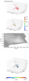 |
Fig. B.5. Same as Fig. B.1 for the overdensity detected at z = 2.69 in the CDFS. |
| In the text | |
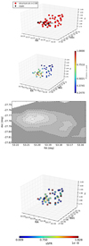 |
Fig. B.6. Same as Fig. B.1 for the overdensity detected at z = 2.80 in the CDFS. |
| In the text | |
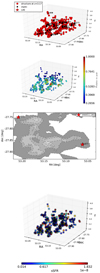 |
Fig. B.7. Same as Fig. B.1 for the overdensity detected at z = 3.17 in the CDFS. |
| In the text | |
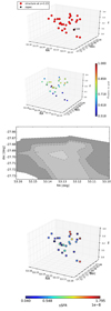 |
Fig. B.8. Same as Fig. B.1 for the overdensity detected at z = 3.23 in the CDFS. |
| In the text | |
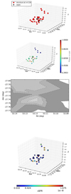 |
Fig. B.9. Same as Fig. B.1 for the overdensity detected at z = 3.29 in the CDFS. |
| In the text | |
|
Fig. B.10. Same as Fig. B.1 for the overdensity detected at z = 3.43 in the CDFS. |
| In the text | |
|
Fig. B.11. Same as Fig. B.1 for the overdensity detected at z = 3.54 in the CDFS. |
| In the text | |
|
Fig. B.12. Same as Fig. B.1 for the overdensity detected at z = 3.55 in the CDFS. |
| In the text | |
|
Fig. B.13. Same as Fig. B.1 for the overdensity detected at z = 3.69 in the CDFS. |
| In the text | |
|
Fig. B.14. Same as Fig. B.1 for the overdensity detected at z = 2.33 in the UDS. |
| In the text | |
|
Fig. B.15. Same as Fig. B.1 for the overdensity detected at z = 3.25 in the UDS. |
| In the text | |
|
Fig. B.16. Same as Fig. B.1 for the overdensity detected at z = 3.25 in the UDS. |
| In the text | |
|
Fig. B.17. Same as Fig. B.1 for the overdensity detected at z = 3.27 in the UDS. |
| In the text | |
|
Fig. B.18. Same as Fig. B.1 for the overdensity detected at z = 3.49 in the UDS. |
| In the text | |
|
Fig. B.19. Same as Fig. B.1 for the overdensity detected at z = 3.51 in the UDS. |
| In the text | |
|
Fig. B.20. Same as Fig. B.1 for the overdensity detected at z = 3.65 in the UDS. |
| In the text | |
|
Fig. B.21. Same as Fig. B.1 for the overdensity detected at z = 3.69 in the UDS. |
| In the text | |
|
Fig. B.22. Same as Fig. B.1 for the overdensity detected at z = 4.01 in the UDS. |
| In the text | |
|
Fig. C.1. As described in the text of this section for the overdensities detected at z = 2.29 (leftpanels) and z = 2.30 (rightpanels) in the CDFS. |
| In the text | |
|
Fig. C.2. As described in the text of this section for the overdensities detected at z = 2.80 (leftpanels) and z = 3.17 (rightpanels) in the CDFS. |
| In the text | |
|
Fig. C.3. As described in the text of this section for the overdensities detected at z = 3.54 (leftpanels) and z = 3.55 (rightpanels) in the CDFS. |
| In the text | |
|
Fig. C.4. As described in the text of this section for the overdensities detected at z = 2.33 (leftpanels) and z = 3.25 (rightpanels) in the UDS. |
| In the text | |
|
Fig. C.5. As described in the text of this section for the overdensities detected at z = 3.27 (leftpanels) and z = 3.65 (rightpanels) in the UDS. |
| In the text | |
|
Fig. D.1. As described in the text of this section for the overdensities detected at z = 2.29 (leftpanels) and z = 2.30 (rightpanels) in the CDFS. |
| In the text | |
|
Fig. D.2. As described in the text of this section for the overdensities detected at z = 2.80 (leftpanels) and z = 3.17 (rightpanels) in the CDFS. |
| In the text | |
|
Fig. D.3. As described in the text of this section for the overdensities detected at z = 3.54 (leftpanels) and z = 3.55 (rightpanels) in the CDFS. |
| In the text | |
|
Fig. D.4. As described in the text of this section for the overdensities detected at z = 2.33 (leftpanels) and z = 3.25 (rightpanels) in the UDS. |
| In the text | |
|
Fig. D.5. As described in the text of this section for the overdensities detected at z = 3.27 (leftpanels) and z = 3.65 (rightpanels) in the UDS. |
| In the text | |
Current usage metrics show cumulative count of Article Views (full-text article views including HTML views, PDF and ePub downloads, according to the available data) and Abstracts Views on Vision4Press platform.
Data correspond to usage on the plateform after 2015. The current usage metrics is available 48-96 hours after online publication and is updated daily on week days.
Initial download of the metrics may take a while.