| Issue |
A&A
Volume 638, June 2020
|
|
|---|---|---|
| Article Number | A88 | |
| Number of page(s) | 18 | |
| Section | Planets and planetary systems | |
| DOI | https://doi.org/10.1051/0004-6361/202037720 | |
| Published online | 18 June 2020 | |
Pebble-driven planet formation around very low-mass stars and brown dwarfs
1
Lund Observatory, Department of Astronomy and Theoretical Physics, Lund University,
Box 43,
22100
Lund,
Sweden
e-mail: This email address is being protected from spambots. You need JavaScript enabled to view it.
2
Lunar and Planetary Laboratory, University of Arizona,
Tucson,
AZ
85721,
USA
3
Max-Planck-Institut für Astronomie,
Königstuhl 17,
69117
Heidelberg,
Germany
Received:
13
February
2020
Accepted:
14
April
2020
Abstract
We conduct a pebble-driven planet population synthesis study to investigate the formation of planets around very low-mass stars and brown dwarfs in the (sub)stellar mass range between 0.01 M⊙ and 0.1 M⊙. Based on the extrapolation of numerical simulations of planetesimal formation by the streaming instability, we obtain the characteristic mass of the planetesimals and the initial mass of the protoplanet (largest body from the planetesimal populations), in either the early self-gravitating phase or the later non-self-gravitating phase of the protoplanetary disk evolution. We find that the initial protoplanets form with masses that increase with host mass and orbital distance, and decrease with age. Around late M-dwarfs of 0.1 M⊙, these protoplanets can grow up to Earth-mass planets by pebble accretion. However, around brown dwarfs of 0.01 M⊙, planets do not grow to the masses that are greater than Mars when the initial protoplanets are born early in self-gravitating disks, and their growth stalls at around 0.01 Earth-mass when they are born late in non-self-gravitating disks. Around these low-mass stars and brown dwarfs we find no channel for gas giant planet formation because the solid cores remain too small. When the initial protoplanets form only at the water-ice line, the final planets typically have ≳15% water mass fraction. Alternatively, when the initial protoplanets form log-uniformly distributed over the entire protoplanetary disk, the final planets are either very water rich (water mass fraction ≳15%) or entirely rocky (water mass fraction ≲5%).
Key words: methods: numerical / planets and satellites: formation
© ESO 2020
1 Introduction
Brown dwarfs are substellar objects in the mass range between 13 and 80 Jupiter masses (approximately 0.013 and 0.08 M⊙). They fall below the stable hydrogen-burning mass limit but can sustain deuterium and lithium nuclear fusion. These brown dwarfs, together with very low-mass hydrogen-burning M dwarf stars of masses ≲0.1 M⊙ (effective temperature below 2700 K, stellar type later than M7) are referred to as ultra-cool dwarfs (UCDs). Noticeably, the UCDs represent a significant fraction (~15−30%) of stars in the galaxy (Kroupa 2001; Chabrier 2003; Kirkpatrick et al. 2012; Mužić et al. 2017).
The evidence for dust disks around young brown dwarfs was first probed by the presence of an infrared excess in the spectral energy distribution (SED; Comerón et al. 2000; Natta & Testi 2001; Pascucci et al. 2003), and later by the detection of (sub)millimeter emission (Klein et al. 2003) from the cold dust. Both dust continuum emission and CO molecular line emission were later on observed for a large sample of brown dwarf disks through surveys with the Atacama Large Millimeter/submillimeter Array (ALMA; Ricci et al. 2012, 2014; Testi et al. 2016). Based on the infrared spectroscopic surveys by the Spitzer space telescope, Apai et al. (2005) found that grain growth, crystallization, and vertical settling all take place in such young brown dwarf disks. Furthermore, multi-wavelength observations resolve low spectral indices for these brown dwarf disks, implying dust grains already grow up to millimeter (mm) and centimeter (cm) sizes (Ricci et al. 2010, 2014, 2017)1. All these mentioned brown dwarf disk studies, combined with the vast literature on disks around more massive stars (Przygodda et al. 2003; Natta et al. 2004; Pérez et al. 2015; Tazzari et al. 2016), convincingly support that the robustness of the first step of planet formation, grain growth, is ubiquitous among different young (sub)stellar environments, extending down to the brown dwarf regime.
Spectroscopic measurements of mass accretion rates onto brown dwarfs have found Ṁg of the order of 10−12M⊙ yr−1 (Muzerolle et al. 2005; Mohanty et al. 2005; Herczeg et al. 2009), which is much lower than the nominal value for solar-mass stars of 10−8M⊙ yr−1 (Hartmann et al. 1998; Garcia Lopez et al. 2006; Manara et al. 2012), implying a decreasing trend of mass accretion rate with (sub)stellar mass down to the brown dwarf regime. Brown dwarfs also have protoplanetary disks of relatively low mass (Andrews et al. 2013; Mohanty et al. 2013). Recent studies plausibly suggest a lower disk-to-star mass ratio (Md ∕M⋆) for disks around brown dwarfs and very low-mass stars compared to those around T Tauri stars (Harvey et al. 2012; Pascucci et al. 2016; Testi et al. 2016).
The lifetime of disks around M dwarfs and brown dwarfs is typically longer than the lifetime of those around high-mass stars (Carpenter et al. 2006; Scholz et al. 2007; Riaz et al. 2012). The stellar multiplicity however exhibits the opposite trend. The binary frequency is ~ 10% for brown dwarfs, and this fraction increases with stellar mass, up to ~50% for solar-type stars (Burgasser et al. 2006; Ahmic et al. 2007; Lafrenière et al. 2008; Joergens 2008; Raghavan et al. 2010; Fontanive et al. 2018).
Young solar-mass stars contract over a few tens of Myr to settle down to the main-sequence where they initiate nuclear fusion. However, the Kelvin–Helmholtz contraction timescale for UCDs is much longer (100 Myr to a few Gyr, Chabrier & Baraffe 1997). As UCDs contract and cool down, their luminosities become more than two orders of magnitude fainter (Chabrier & Baraffe 1997; Burrows et al. 1997). Eventually, they stop shrinking when the gas is dense enough that electrons become degenerate in the interior. Besides, these UCDs are also faster rotators, with a typical rotation period of 0.5− 1 day (Herbst et al. 2007). The magnetic B-field strengths of these low-mass objects are comparable to those of T Tauri stars, reaching the kilogauss level (Reiners 2012), while their magnetic activities can last longer compared to those of T Tauri stars (Reiners & Christensen 2010).
Current exoplanet surveys, such as the MEarth project (Nutzman & Charbonneau 2008), TESS (Transiting Exoplanets Survey Satellite, Ricker et al. 2015), SPECULOOS (search for Habitable planets Eclipsing Ultra-cool Stars, Gillon et al. 2013; Burdanov et al. 2018), CARMENES (Calar Alto high-Resolution search for M dwarfs with Exoearths with Near-infrared and optical Echelle Spectrographs, Quirrenbach et al. 2018), and the Project EDEN (ExoEarth Discovery and Exploration Network) transit survey are currently operational to probe which types of planets and how frequent they are around stars in the ultra-cool dwarf regime. The planets discovered around TRAPPIST-1 (Gillon et al. 2016, 2017) and Teegarden’s star (Zechmeister et al. 2019) are two known systems in these pioneering explorations. These two hosts are both late M-dwarfs, and no planets have yet been detected by radial velocity/transit around brown dwarfs.
From a theoretical point of view, the fundamental question to address is whether and how planets form in these low-mass (sub)stellar systems. As stated, various host and disk properties for UCDs exhibit certain similarities to and diversities from high mass stars. In Liu et al. (2019a) we constructed a pebble-driven planet formation model and focused on the growth and migration of planets around stars from late M-dwarfs to solar mass. We found a linear correlation between the characteristic planet mass (the maximum planet core mass) and the mass of the stellar host2. In this work we extend our population synthesis study to a lower (sub)stellar mass range, from 0.01 M⊙ (≈ 10 MJup) to 0.1 M⊙. We present the first results of population synthesis simulations for planet formation around ultra-cool dwarfs from the pebble accretion perspective. Specifically, we aim to explore how the planet mass correlates with the host’s mass in this regime.
The paper is designed as follows. Section 2 briefly reviews our previous model (Liu et al. 2019a) and describes three major improvements from this work. The growth tracks of individual protoplanets (planet mass vs. semi-major axis) around UCD disks are illustrated in Sect. 3. We simulate the growth and migration of a large number of protoplanets by Monto Carlo sampling their initial conditions. In Sect. 4 we present the resulting planets with their masses, semi-major axes and water fractions. We summarize our findings and discuss the implications in Sect. 5.
2 Planet formation model
Liu et al. (2019a) constructed a pebble-driven planet formation population synthesis model; details of the model can be found in their Sect. 2. The most important equations of the disk model are recapitulated in Appendix A. In this study we include three major improvements compared to the previous one. In Sect. 2.1 we introduce the new adopted disk accretion rate based on observations. The pebble size is adopted to be the same as Liu et al. (2019a), which is evaluated in Sect. 2.2. The dependences of the luminosity on time and (sub)stellar mass are considered in Sect. 2.3. The characteristic planetesimal mass and initial mass of the protoplanet are obtained in Sect. 2.4 and Sect. 2.5, based on the extrapolation of planetesimal masses from streaming instability simulations presented inthe literature. In particular, we emphasize the influence of the host’s mass on these key physical quantities.
2.1 Disk properties
An analytical self-similar solution for the viscous disk evolution (Lynden-Bell & Pringle 1974; Hartmann et al. 1998)was used in our previous work. Alternatively, here we adopt a fitting formula of Ṁg (M⋆, t) from Manara et al. (2012), based on observations of a large sample of sources in Orion Nebula Cluster, which gives
![Mathematical equation: \begin{equation*} \begin{split} \log\left[\frac{\dot M_{\textrm{g}}}{M_{\odot}\,\textrm{yr}^{-1}} \right] = & {-}5.12 -0.46 \log\left[\frac{t}{ \ \textrm{yr}}\right] -5.75\log\left[\frac{ M_{\star}}{ \ M_{\odot} }\right] \\[3pt] & +1.17 \log\left[\frac{t}{ \ \textrm{yr}}\right]\log\left[\frac{ M_{\star}}{ \ M_{\odot} }\right], \end{split}\end{equation*}](/articles/aa/full_html/2020/06/aa37720-20/aa37720-20-eq1.png) (1)
(1)
where M⋆ is the mass of central host, and t is the age of the disk. Since the age determination for young protostars is highly uncertain during the early infall stage, as pointed out by Manara et al. (2012), Eq. (1) is invalid when the disk is younger than 0.3 Myr. We assume that Ṁg remains a constant when t < 0.3 Myr. In their sample, the mass of the central host ranges from 2 M⊙ to 0.05 M⊙. We assume here that the above equation can be extrapolated down to the very low-mass brown dwarf of 0.01 M⊙.
In contrast to this approach, Liu et al. (2019a) assumed a viscously evolving disk, where Ṁg depends on time as t≈−3∕2. Although several studies have attempted to link the observed disks with viscous accretion theory, the connection has not yet been firmly established (e.g., Lodato et al. 2017; Mulders et al. 2017; Najita & Bergin 2018). Nonetheless, the disk evolution Ṁg (M⋆, t) from this work is purely based on observations.
Figure 1a shows the evolution of disk accretion rates for central hosts of 0.01 M⊙ (= 10 MJup), 0.1 M⊙, and 1 M⊙, respectively. There are two distinctive features: First, disks around less massive stars have lower accretion rates. Second and more importantly, disk accretion rates around less massive stars also decrease more rapidly. We also note that, based on disk accretion rates measured from X-shooter spectrograph, more recent studies suggest a steeper Ṁg −M⋆ for lower mass stars (Manara et al. 2017; Alcalá et al. 2017), which appears in agreement with faster disk evolution around these stars. We find in Fig. 1a that at the beginning, Ṁg = 10−9 M⊙ yr−1 in a brown dwarf disk, which is a factor of 5 and 30 times lower than the accretion rates in 0.1 M⊙ and 1 M⊙ star disks. However, after 2 Myr, the disk accretion rate in the brown dwarf disk drops by more than two orders of magnitude, while Ṁg ≃ 10−8 M⊙ yr−1 for the solar-mass star, which is only reduced by a factor of three compared to its initial value.
We can calculate the gas disk mass (Md) by integrating Ṁg over time (chooset = 10 Myr) for the host of specific M⋆. By doing so,we need to assume that the disk material is mainly accreted onto the central star, rather than carried away by a disk wind. It is true for viscous disks where most gas in the disk is accreted inward while a small amount of gas spreads far away to conserve theangular momentum (Lynden-Bell & Pringle 1974). Therefore, we can link the mass accretion rate for the inner disk region to the whole disk mass.
The results are illustrated in Fig. 1b. We find that at an early stage the disk mass tends to scale linearly with the mass of the central host. However, since the disk around low-mass stars/brown dwarfs evolves rapidly, at t ~ 1−3 Myr the disk mass is roughly proportional to the mass of the host squared ( ). This inferred stellar mass square dependence also matches the measurements of disk accretion rates in the Chamaeleon I star forming region (Manara et al. 2016), which have similar ages of 1− 3 Myr. The early linear Md−M⋆ correlation (t ≲ 0.5 Myr) could be partially due to the constant Ṁg assumption in the short embedded phase. Nevertheless, the fact that the Md −M⋆ relation increases steeply with time always holds as long as the disk evolves more rapidly for very low-mass stars/brown dwarfs than for higher-mass stars. We also note that such time-dependence is not only observed for the gas component (inferred from Ṁg). There is clear evidence that the correlation between the dust mass and stellar mass becomes steeper with time as well (Pascucci et al. 2016; Ansdell et al. 2017).
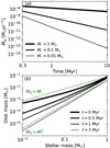 |
Fig. 1 (a) Time evolution of disk accretion rates among three stars of different masses, based on Eq. (6) of Manara et al. (2012). The disk accretion rate drops faster with decreasing mass of the central object. (b) Disk mass vs. (sub)stellar mass at different times, based on Ṁg measurements of Manara et al. (2012). The solid lines from thick to thin represent the ages of systems, from 0 to 0.5, 1, and 3 Myr. The green dashed lines correspond to the linear and quadratic relation between the disk mass and the stellar mass. When the disk is ≲1 Myr old, Md ∝ M⋆, while |

2.2 Dust growth
Similar to Liu et al. (2019a), we also assume in this paper that dust grains can efficiently grow to mm sizes. This characteristic size is motivated from two aspects. Firstly, the mm spectral index measured for the disks around stars of various masses (including brown dwarfs) is much lower than the typical interstellar medium (ISM) value. This indicates that the grains already grow to such sizes in protoplanetary disks over a wide range of ages (Draine 2006; Ricci et al. 2014, 2017; Pérez et al. 2015; Tazzari et al. 2016; Pinilla et al. 2017). Secondly, Zsom et al. (2010) studied the coagulation of silicate dust aggregates in protoplanetary disks based on the collision outcomes from laboratory experiments (Güttler et al. 2010). They found that particles stall at roughly mm sizes due to the bouncing barrier. The sticking of particles is determined by the surface energy, which correlates with the material properties. Recently, Musiolik & Wurm (2019) reported that the surface energy of ice aggregates is comparable to that of silicates when the disk temperature is lower than 180 K. If this is true, the growth pattern and the bouncing-limited size would be quite similar for these two types of dust grains.
Rather than build a sophisticated model for dust growth and radial drift (Birnstiel et al. 2012), here we assume that the pebble mass flux (Ṁpeb) generated from the dust reservoir in the outer disk regions is attached to the gas flow with a constant mass flux ratio, such that ξ ≡ Ṁpeb∕Ṁg does not change with time (Johansen et al. 2019). Particles of very low Stokes numbers are well-coupled to the disk gas. The gas and dust particles drift inward together with the same velocities, and therefore ξ remains equal to the initial disk metallicity. When the Stokes number is high, pebbles radially drift faster than the disk gas. In this case, in order to maintain a constant flux ratio, Σpeb∕Σg becomes lower than the nominal disk metallicity (the pebble surface density is reduced). The mm-sized pebbles in disks around GK and early M-dwarfs are typically in the former circumstance, while such pebbles in disks around very low-mass stars and brown dwarfs could be in the latter circumstance, especially at the late evolutional stage.
We would like to point out that the above constant mass flux ratio assumption is a global concept. Even though the global Σpeb ∕Σg is no higher than the disk metallicity under this assumption, the density of the solids can still be enriched at local disk locations due to a variety of mechanisms. For instance, several studies proposed that the solid-to-gas ratio can be enhanced at the water-ice line (Ros & Johansen 2013; Schoonenberg & Ormel 2017; Dra̧żkowska & Alibert 2017). This is because the water vapor is released by the inward-drifting icy pebbles when these pebbles cross the ice line. The water vapor diffuses back to the low-density region exterior to the ice line and re-condenses onto the icy pebbles. This process increases Σpeb ∕Σg locally and triggers the streaming instability to form planetesimals at the water-ice line. Furthermore, Lenz et al. (2019) proposed that the dust particles can be trapped at pressure bumps, which may exist over a wide region of the disk due to hydrodynamical and/or magnetic turbulence. Similarly, such places of sufficiently high Σpeb ∕Σg can also facilitate the planetesimal formation. These ideas also motivate our further hypothesis on the birth locations of the protoplanets in the population synthesis study in Sect. 4.
On the other hand, the constant flux ratio assumption also neglects the reduction of Ṁpeb due to planet pebble accretion. We give the reason for this simplification as follows. The typical gas disk mass is 1− 10% of the stellar mass (Fig. 1), resulting in a mass ratio between disk pebbles and the central host of ≈ 10−4−10−3. For comparison, we found that the mass ratio between the pebbles accreted by the planet and the central host ranges from zero to a maximum of3 × 10−5 (see Fig. 7). We find that even in cases where the planet reaches the pebble isolation mass of Mp ∕M⋆ ~ 3 × 10⁻⁵, the fraction of pebble accreted by the planet is still <10%. Most pebbles in disks are actually accreted to the central hosts rather than accreted by planets. Our constant flux ratio assumption is therefore justified.
We present the results for 1 mm size pebbles in the main paper. In addition, we also consider a case that includes the combined effects of bouncing, fragmentation, and radial drift. The corresponding results are summarized in Appendix C.2. These two particle size assumptions nevertheless result in very similar outcomes.
Based on Eqs. (A.1) and (A.4) we write the Stokes number of 1 mm particles in the Epstein regime:
![Mathematical equation: \begin{align*} \tau_{\textrm{s}}&= \sqrt{2 \pi} \frac{ R_{\textrm{peb}} \rho_{\bullet}}{ \Sigma_{\textrm{g}}} \nonumber\\ &= \begin{cases} {\displaystyle 0.007 \left(\frac{\dot M_{\textrm{g}}}{10^{-9}\,M_{\odot}\,\textrm{yr}^{-1}} \right)^{-\frac{1}{3}} \left(\frac{\rho_{\bullet}}{1.5 \textrm{\ g\,cm}^{-3} } \right) \left(\frac{R_{\textrm{peb}}}{1 \textrm{\ mm} } \right) } \\ \hspace{6.5cm} [r = r_{\textrm{ice}}], \vspace{0.6cm} \\ {\displaystyle 0.2 \left(\frac{\dot M_{\textrm{g}}}{10^{-9}\,M_{\odot}\,\textrm{yr}^{-1}} \right)^{-1} \left(\frac{M_{\star}}{0.1 \ M_{\odot}} \right)^{-\frac{9}{14}} \left(\frac{L_{\star}}{0.01 \ L_{\odot}} \right)^{\frac{2}{7}} } \\ \hspace{6.cm} [r = 10 \,\textrm{AU}], \end{cases} \end{align*}](/articles/aa/full_html/2020/06/aa37720-20/aa37720-20-eq3.png) (2)
(2)
where Rpeb and ρ∙ are the physical radius and internal density of the pebble. The first and second rows of the above equation compute the values evaluated at the water-ice line location in the inner viscously heated disk region and at 10 AU in the stellar irradiation disk region, respectively.
For particles of fixed-size, the Stokes number is inversely proportional to the surface density of the disk gas. As the disk masses decrease with both the mass of the central host and time, the Stokes number therefore increases with these two quantities. This is clearly shown in Fig. 2, which illustrates the evolution of Stokes numbers for 1 mm size pebbles at the water-ice line (orange) and at 10 AU (blue) in disks around different mass hosts. For disks around solar-mass stars, no matter where pebbles are, τs always remains lower than 0.03. However, for disks around brown dwarfs of 0.01 M⊙, τs approaches unity for pebbles at the ice line when t ≃ 7 Myr, while for pebbles at 10 AU, this occurs even at the very early stage when t ≃ 0.5 Myr.
The Stokes number determines the efficiency of pebble accretion. When the planet mass is low, the pebble accretion efficiency decreases with τs in the 3D regime where the planet accretion radius is smaller than the vertical layer of the pebbles (Morbidelli et al. 2015; Ormel & Liu 2018). As the planet grows, it enters the 2D accretion regime. In this situation, the pebble accretion efficiency increases with τs (Lambrechts & Johansen 2014; Liu & Ormel 2018). The above analysis holds as long as the pebbles are marginally coupled to the disk gas, and therefore gas drag is important during the pebble-planet interaction (10−3 ≲ τs ≲ 1). However, when τs is much greater thanunity, gas drag is negligible during pebble-planet encounters, and pebbles are more aerodynamically similar to planetesimals. In this case, the actual accretion rate drops substantially (Ormel & Klahr 2010). Therefore, the preferred Stokes number for pebble accretion ranges from 10−3 to 1.
Noticeably, as illustrated in Figs. 1 and 2, we find that the protoplanets formed at wide orbits around low-mass hosts, especially brown dwarfs, would have difficulty in growing significantly in mass by accreting pebbles. This is because disks around these low-mass objects deplete rapidly in both solids and gas. Furthermore, mm-sized pebbles in disks around such hosts have Stokes numbers larger than unity, and the corresponding pebble accretion turns out to be very inefficient.
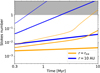 |
Fig. 2 Time evolution of Stokes numbers of mm-sized particles at r = rice (orange) andat r = 10 AU (blue) among three hosts of different masses. The thickness of lines represents the masses of the hosts, 1 M⊙, 0.1 M⊙, and 0.01 M⊙, respectively.The Stokes number quickly increases past unity at the distant disk location around low-mass stars, resulting in inefficientpebble accretion. |
2.3 Stellar properties
The second modification compared to our previous study is our adoption of the time evolution of the luminosity of the central object. In Liu et al. (2019a) we assumed that the luminosity of a young star does not evolve during the short disk lifetime (≲ 10 Myr), and therefore, it only correlates with the stellar mass as  , where β is parameterized to be either 2 or 1 for the pre-main sequence stars. As an improvement, here we adopt a theoretical calculation of L⋆ (M⋆, t) from Baraffe et al. (2003, 2015), who use state-of-the-art evolutionary models that compute L⋆ (M⋆, t) for stars from solar-mass to brown dwarfs below the hydrogen-burning limit.
The time and (sub)stellar mass dependencies can be seen in Fig. 3. For hosts younger than 10 Myr, we verify that  is still a good approximation. After that, the luminosity tends to follow a cubic or fourth power correlation with the mass of the host. It is worth mentioning that this time-dependent variation is due to the much slower contraction for lower mass stars. For comparison, the contraction of solar-mass stars roughly takes a few tens of millions of years, while this can last for 108 –109 yr for UCDs. A complete contour map of L⋆(M⋆, t) is provided in Fig. B.1.
Young UCDs are fast rotators (Herbst et al. 2007). We approximate the inner edge of the disk to the corotation radius of the central host with a typical spin period P⋆ of one day, which can be expressed as
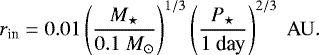 (3)
(3)
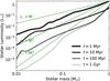 |
Fig. 3 Time and (sub)stellar mass dependencies on the luminosity of the host based on the evolutionary model of Baraffe et al. (2003, 2015). The solid lines from thick to thin indicate the systems’ ages from 1 Myr to 10 Myr, 100 Myr, and 1 Gyr. Thegreen dashed lines correspond to a linear, quadratic, cubic, and fourth power correlation between the luminosity and mass. We find that when the central host is younger than 10 Myr, |


2.4 Derivation of the characteristic planetesimal mass from streaming instability simulations
Streaming instability is a powerful mechanism that forms planetesimals by directly collapsing a swarm of mm-sized pebbles (Youdin & Goodman 2005). Numerous numerical simulations show the robustness of this mechanism for generating planetesimals (Johansen et al. 2007, 2012; Bai & Stone 2010; Simon et al. 2016; Schäfer et al. 2017; Abod et al. 2019; Li et al. 2019). These planetesimals have a top-heavy mass distribution. The characteristic planetesimal size is roughly 100 km in the asteroid belt region (2−3 AU) around a solar-mass star (Johansen et al. 2015; Simon et al. 2016; Schäfer et al. 2017).
Simulations of streaming instability are performed in a shearing box, where the code units are typically set as  . The midplane gas density ρg, the gas disk scale height H, and the Keplerian angular frequency
  correspond to the units of density, length, and time, respectively, where G is the gravitational constant and all these quantities are measured at a radial distance r from the central star. The unit of mass is given by
  .
.
The gasdensity is set by the dimensionless gravity parameter
 (4)
(4)
where γ measures the relative strength between the self-gravity and tidal shear, which depends on the gas density ρg, the stellar mass M⋆, and the radial distance r. The mass unit can in turn be written as
 (5)
(5)
where disk aspect ratio h = H∕r. We note that the variation of γ is equivalent to the change of ρg for fixed r and M⋆.
In the streaming instability simulations, planetesimal masses are measured in the code unit (in terms of  ). These masses are expected to follow the same scaling laws when
  varies. This means we could extrapolate and obtain the physical mass of the planetesimal when realistic ρg, M⋆, and r are given.
We propose that the characteristic planetesimal mass can be written as
 (6)
(6)
There are four key physical quantities that regulate the gravitationally collapsing of planetesimals, and therefore set the control function f. We give these quantities in a dimensionless manner as follows. The radial pressure gradient parameter that measures the sub-Keplerian gas velocity is
 (7)
(7)
where η = −h2(∂ln P∕∂ln r)∕2 = (2 − s − q)h2∕2, P is the gas pressure, s, q are the power law indexes of the gas surface density and disk aspect ratio, respectively. The Stokes number that represents the aerodynamical size of the particles can be written as
 (8)
(8)
where tstop is the stopping time of the particle, The metallicity (the surface density ratio between particles and gas) is given by
 (9)
(9)
The last key physical quantity is γ, which describes the strength of the self-gravity.
We assume that f(Π, γ, τs, Z) is composed of a series of power laws
 (10)
(10)
where a, b, c can be principally obtained from streaming instability simulations. Physically, Z and γ (corresponding to the gas density) together represent the disk solid density, a fundamental quantity that sets the collapse of the pebble clumps and formation of the planetesimals. We expect these two follow the same power-law dependence in f. Equation (6) can be rewritten as
 (11)
(11)
We would like to note that Mpl ∝ γa+1 since  also linearly scales with γ (Eq. (5)). Importantly, the preceding condition for the above formula is to trigger filament formation by the streaming instability in the first place. This requires a certain range of disk metallicities, the Stokes numbers and disk pressure gradients (Bai & Stone 2010; Carrera et al. 2015; Yang et al. 2017).
From Fig. 3 of Simon et al. (2017), we find that the planetesimal mass depends very little on the Stokes number of the pebbles. We therefore drop the τs dependence on Mpl hereafter. The characteristic mass of the planetesimal can be expressed as
 (12)
(12)
Again, we note that Z represents the local metallicity in the above equation. As discussed in Sect. 2.2, this value can differ from the global disk metallicity due to different dust concentration mechanisms.
Converting the code unit into the physical unit based on Eqs. (5) and (12), we therefore obtain
 (13)
(13)
There are three unknown parameters a, b, and C in Eq. (12). We explain how we choose these values as follows. Both Johansen et al. (2012) and Simon et al. (2016) explore the role of the self-gravity parameter γ on the final planetesimal masses. The inferred power-law index a is between 0 and 1 (Fig. 13 of Johansen et al. 2012 and Fig. 9 of Simon et al. 2016). We find that a medium value of a = 0.5 is slightly preferred3. This latter value causes Mpl to increase super-linearly with γ in Eq. (13). On the other hand, different disk pressure gradients Π are explored in Abod et al. (2019). The inferred b is no larger than 1 and can be close to 0 (b ~ 0−1, their Fig. 8). This Π dependence on Mpl also seems to be nonmonotonic. For a conservative choice, we adopt b = 0 here. This leads to Mpl ∝ h3. We choose C = 5 × 10⁻⁵ based on Table 2 of Schäfer et al. (2017). As will be demonstrated below, our proposed characteristic mass based on the above adopted values is in reasonably good agreement with other numerical studies.
The characteristic mass comparison between the literature studies and our Eq. (12) is illustrated in Fig. 4. In streaming instability simulations, the cumulative mass distribution of the forming planetesimals is most frequently fitted by a power law plus an exponential decay, ![Mathematical equation: $N_{>}(M) \,{=}\, kM^{-\alpha_1}\exp[-(M/M_{\textrm{exp}})^{\beta_1}]$](/articles/aa/full_html/2020/06/aa37720-20/aa37720-20-eq23.png) . There are two different approaches for the above fitting. One is the simply tapered power law (STPL), where k and α1 are two free parameters, and β1 is fixed to be either 4∕3 (Johansen et al. 2015) or 1 (Abod et al. 2019; Li et al. 2019). The other is the variably tapered power law (VTPW), where β1 is an additional free parameter that needs to be fitted (Schäfer et al. 2017; Li et al. 2019). Apart from these exponentially tapered power laws, a single power law (SPL) is used in Simon et al. (2016), and a broken power law (BPL) is explored in Li et al. (2019; their Eq. (23)). The characteristic masses are adopted as Mexp in exponentially tapered power laws and Mbr (turnover mass) in the broken power law. For the single power law fitting, we mark the highest planetesimal mass as an indicator of the upperlimit of the characteristic mass. The data used for this comparison are listed in Table 1.
. There are two different approaches for the above fitting. One is the simply tapered power law (STPL), where k and α1 are two free parameters, and β1 is fixed to be either 4∕3 (Johansen et al. 2015) or 1 (Abod et al. 2019; Li et al. 2019). The other is the variably tapered power law (VTPW), where β1 is an additional free parameter that needs to be fitted (Schäfer et al. 2017; Li et al. 2019). Apart from these exponentially tapered power laws, a single power law (SPL) is used in Simon et al. (2016), and a broken power law (BPL) is explored in Li et al. (2019; their Eq. (23)). The characteristic masses are adopted as Mexp in exponentially tapered power laws and Mbr (turnover mass) in the broken power law. For the single power law fitting, we mark the highest planetesimal mass as an indicator of the upperlimit of the characteristic mass. The data used for this comparison are listed in Table 1.
We find that our proposed characteristic mass in Eq. (12) is in good agreement with values in the literature. As can be seen in Fig. 4, our predicted value is lower than the characteristic mass in Johansen et al. (2015) by a factor of 2− 3 (pink triangle) but is in relatively good agreement with other studies. The above degree of consistence is impressive, since Π, γ, τs and Z are varied over orders of magnitude among these studies (see Table 1). Furthermore, different fitting formulas and therefore characteristic mass indicators (Mexp and Mbr) are adopted in the literature. These indicators might differ by a factor of a few from each other even based on the same fitting data (see magenta symbols in Fig. 4). In addition, different planetesimal-finding algorithms among these studies could also induce additional uncertainties in the above fitting masses. Overall, we are confident about the values chosen here (a = 0.5, b = 0, C = 5 × 10⁻⁵). In future, when more numerical simulations are conducted with different disk and pebble parameters, we will be able to optimisze all these parameters in Eq. (11) based on more advanced best-fit algorithms.
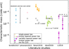 |
Fig. 4 Characteristic mass comparison among literature studies and our Eq. (12) calibrated from the results of Schäfer et al. (2017). The planetesimals obtained from streaming instability simulations are fitted by different distributions, including a single power law (dot), a simply tapered power law (triangle), a variably tapered power law (diamond), and a broken power law (square). The details of these fitting formulas are explained in the main text. The pink, orange, blue, green, and magenta refer to the studies of Johansen et al. (2015), Simon et al. (2016), Schäfer et al. (2017), Abod et al. (2019), and Li et al. (2019), respectively. We note that the orange dots only refer to the maximum masses of the planetesimals; we add the downside arrows to indicate that the characteristic masses should be lower than these values. The characteristic masses obtained in each set ofparameters are shown in symbols with the same x-axis (see Table 1). We note that Z, γ, Π, and τs are different by orders of magnitude among these numerical studies. Our Eq. (12) agrees reasonably well with the fitting characteristic masses found in these studies. |
2.5 Initial mass of the protoplanets
Based on streaming instability simulations (e.g., Schäfer et al. 2017), the mass of the largest body M0 is typically about two to three orders of magnitude higher than the characteristic mass (see Fig. 7 in Liu et al. 2019b). As demonstrated in Liu et al. (2019b), the most massive planetesimal would dominate the following mass growth and dynamical evolution of the whole population. In this population synthesis study, we adopt the largest planetesimal formed by streaming instability as our starting point, and we refer to it as the protoplanet hereafter. The subsequent growth and migration of one single protoplanet is investigated in this study.
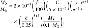
Assuming that the disk solids are locally enriched in order to satisfy the Z criterion, we drop the Z dependence in Eq. (13) hereafter. The mass of the initial protoplanet is given by
 (14)
(14)
where fplt is the ratio between the maximum mass and the characteristic mass. In this study, we set fplt = 400, a = 0.5, b = 0, and C = 5 × 10⁻⁵ to be the fiducial values.
Since γ is a disk-related parameter, the key issue is to understand how γ scales with M⋆ and r under different disk conditions. Two types of disks (or two disk evolutional phases) are explored, self-gravitating and non-self-gravitating, which result in γ being either equal to 1 or much less than 1, respectively.
First, we consider the case where the disk is everywhere gravitationally unstable (Toomre Q ≈ 1). This requires a young and massive disk. In this situation, γ = 1 and the mass of the forming protoplanet is independent of γ. Therefore, we do not need to know the gas density ρg directly, since its value is encoded in γ. As can be seen from Eq. (14), the protoplanet’s mass exhibits a similar scaling to that of the pebble isolation mass, also proportional to h3M⋆ (Lambrechts et al. 2014; Bitsch et al. 2018).
On the other hand, during a later phase when the disk is non-self-gravitating, γ ≠ 1 and the actual value depends on the gas surface density. We then calculate γ based on our two-component disk model with an inner viscously heated region and an outer stellar irradiated region (see Appendix A). In a steady state viscous accretion disk, the gas surface density is related to the mass accretion rate and viscosity such that Ṁg =3πΣgν, where  , αg represents the angular momentum transfer coefficient and cs is the gas sound speed. Based on the definition of γ, we derive that
  in this case. This means that with the given disk temperature and αg, γ is proportional to Ṁg.
For the non-self-gravitating disk, after the protoplanets form, the disk evolution follows the nominal two-component model, where the disk surface density and aspect ratio are adopted from Eqs. (A.1) and (A.2) and the time evolution is based on Eq. (1). However, how ρg evolves in a self-gravitating disk is a more subtle issue, which relies on additional assumptions. In principle, ρg is higher in a self-gravitating disk. Even though a young disk is self-gravitating at early times, its density decreases and the disk finally evolves into the non-self-gravitating state. Here we assume that once protoplanets form in a self-gravitating disk, the density quickly adjusts to that of the non-self-gravitating disk. This means that ρg is the same forthese two types of disks after the protoplanet formation. Therefore, the key difference is the birth masses of protoplanets. Such a treatment is conservative for the case of self-gravitating disks. However, the advantage is that the model is reasonably simplified and no additional parameters are needed.
Figure 5a shows the mass of the protoplanet M0 formed by streaming instability as a function of the disk location either in a self-gravitating disk (γ = 1, cyan) or in a non-self-gravitating disk (γ ≠ 1, red) around a 0.1 M⊙ star. The solid and dashed lines correspond to the formation time of the protoplanet at t = 0 Myr and 3 Myr, respectively. The black line represents the pebble isolation mass for comparison. We can see clearly that the initial protoplanet has the same mass scaling as the pebble isolation mass in a self-gravitating disk. When the protoplanet forms early (solid cyan), at the inner regions inside 1 AU region, the disk is viscously heated and the aspect ratio is almost independent of the distance (flat disk, Eq. (A.2)), and therefore M0 and Miso are insensitive to the radial distance. At the region further out where the disk is heated by stellar irradiation, the aspect ratio increases as r2∕7 (flaring disk), and the mass of the protoplanet is nearly proportional to r. In a non-self-gravitating disk (γ ≠ 1), M0 additionally depends on γ, which also increases with r. This simply reflects the fact that the disk self-gravity is likely to overwhelm the tidal shear as the radial distance increases. As a result, we find that the mass of the protoplanet increases super-linearly with distance.
We also clearly see how the mass of the protoplanet formed by streaming instability varies with time. When the protoplanet forms late at 3 Myr (dashed), the disk is entirely heated by stellar irradiation, and, as mentioned, the protoplanet’s mass is purely proportional to r in the self-gravitating disk (γ = 1). Since γ decreases with time in the non-self-gravitating disk, the late-forming protoplanet is less massive compared to the one that forms early.
We also plot the mass of the protoplanet as a function of the stellar mass for the above two disks at the water-ice line in Fig. 5b. We find that the mass of the protoplanet increases slowly with stellar mass in the self-gravitating disk, whereas this stellar mass dependence is more pronounced in the non-self-gravitating disk. We explain the reasons for this as follows. First, based on Eqs. (14) and (A.5), M0 (γ = 1) is proportional to  in the early phase when rice resides in the inner viscously heated region. Second, as shown in Fig. 1a, the difference in disk accretion rates among stars of different masses at the early phase is relatively small, implying a weak dependence of M⋆ on Ṁg. Combined with the above two factors, at early times the mass of the protoplanet modestly increases with stellar mass in the self-gravitating disk (solid cyan). Nevertheless, in the non-self-gravitating disk, M0 (γ ≠ 1) additionally correlates with γ. When taking that into account, we find that M0 exhibits a stronger M⋆ dependence in a non-self-gravitating disk than in a self-gravitating disk.
As discussed in Sect. 2.1, Ṁg is roughly proportional to M⋆ at early times, and the Ṁg−M⋆ correlation becomes steeper as disks evolve. We therefore expect that the mass of the late-forming protoplanets has a steeper stellar mass dependence than those formed early. Figure 5b shows that the late-formingprotoplanet is very small in a non-self-gravitating disk around a low-mass host. For instance, M0 (γ ≠ 1) ≃ 10−9 M⊕ when it forms at t = 3 Myr around a 0.1 M⊙ star, corresponding to 10 km in size.
In summary, the mass of the protoplanet generated by streaming instability correlates with the mass of the central host and the disk location. For the same (sub)stellar host, low-mass protoplanets form at close-in orbits while massive ones form at further distances. For the same disk location, low-mass protoplanets form around less-massive brown dwarfs while high-mass protoplanets form around higher mass stars. The above dependencies are more pronounced for the protoplanets that form in late non-self-gravitating disks than for those in early self-gravitating disks.
Characteristic masses from various numerical streaming instability studies.
 |
Fig. 5 Mass of protoplanet M0 (Eq. (14)) formed by streaming instability as a function of radial distance (left) and host mass (right). The cyan and red lines represent the protoplanets in self-gravitating disks (γ = 1) and non-self-gravitating disks (γ ≠ 1), respectively, whereas the black line corresponds to the pebble isolation mass. The birth time of the protoplanet is assumed to be at t = 0 Myr (solid) yr or 3 Myr (dashed). The mass of the central host is 0.1 M⊙ in panel a and the birth location of the protoplanet is at rice in panel b. When protoplanets form by streaming instability, their birth masses increase with both the mass of the central host and radial distance. |
3 Growth track of a single protoplanet
The detailed treatment of planet growth and migration can be found in Sects. 2.2 and 2.3 of Liu et al. (2019a). Here we provide an analytical comparison between the migration and growth of a growing protoplanet around hosts of different masses.
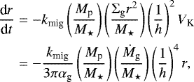
Protoplanets and low-mass planets undergo type I migration (Kley & Nelson 2012), and the corresponding migration rate is
 (15)
(15)
where kmig is the migration coefficient and the latter equation is derived from the steady-state disk assumption where Ṁg = 3πνΣg. It should be noted that we also use two different α parameters in this work, where the global disk viscous angular momentum transfer coefficient αg = 10−2, and the level of the local disk turbulence αt = 10−4. For a given disk accretion rate, αg determines the gas disk surface density, and thus planet migration. On the other hand, planet growth is set by αt which corresponds to the pebble settling and pebble accretion efficiency (see Sect. 2 of Liu et al. 2019a).
The mass accretion rate of a planet in the 2D shear-dominated pebble accretion regime can be found in Liu & Ormel (2018) as
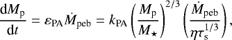 (16)
(16)
where εPA is the pebble accretion efficiency, and kPA = 0.24 is the numerical prefactor in shear-dominated regime.
Based on Eqs. (15) and (16) we can obtain the differential equation for the growth track Mp (r) as (Lambrechts & Johansen 2014; Johansen et al. 2019)
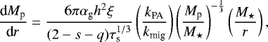 (17)
(17)
where s and q are power-law indexes of disk surface density and aspect ratio. The solution of the above equation is expressed as
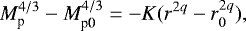 (18)
(18)
where 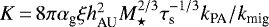 , the subscript 0 means the initial value, and hAU refers to the disk aspect ratio at 1 AU. A larger K indicates the growth is more pronounced than the migration, and the growth track starts to turn over at a higher planet mass (Fig. 6). Within the limit of Mp ≫ Mp0 and r = 0,
 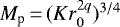 . We can see that the final mass of the planet depends on both K (correlated with the disk metallicity ξ, the stellar mass M⋆, and the particles’ Stokes number τs) and the initial position r0.
Figure 6a shows the growth track for the protoplanets at different disk locations around a 0.01 M⊙ brown dwarf (thin line) and a 0.1 M⊙ star (thick line). We adopt the masses of protoplanets from Eq. (14) for the self-gravitating disk (γ = 1), and assume that in all cases the protoplanets form at t = 0 yr. Based on Eqs. (1) and (A.4), water-ice lines initially reside inside the viscously heated regions, that is, rice = 0.12 AU and 0.55 AU for disks around the corresponding brown dwarf and low-mass star, respectively. We find in Fig. 6a that the turn-over mass when the migration overwhelms the growth is higher for planets around more massive stars. For the case of r0 = rice (orange), the protoplanet around the brown dwarf undergoes substantial migration when Mp ≳ 0.1 M⊕, whereas it starts to migrate at 0.5 M⊕ around the 0.1 M⊙ star. The planet also reaches a higher mass when it orbits around the low-mass star than when it orbits the brown dwarf. As mentioned, both the maximum mass and turn-over point in the growth track are set by K (Eq. (18)), which increases with stellar mass. A similar stellar mass dependence can also be found in Fig. 6a for the cases of r0 < rice (red) and r0 > rice (blue).
Noticeably, the final planet mass strongly depends on its birth location. For systems around 0.1 M⊙ stars, the protoplanets can grow up to 2 M⊕ and 0.5 M⊕ when their birth locations are 1 AU and 0.06 AU. For systems around brown dwarfs, we can see that the growth is insignificant when the protoplanets form at 1 AU. This is because the disks around brown dwarfs deplete rapidly, and therefore the Stokes number of the mm-sized particles becomes very high, resulting in inefficient pebble accretion. Hence, for systems around brown dwarfs, larger planets can only form when their birth locations are close to water-ice lines (r0 ~ rice).
Figure 6b shows the evolution of the ice line (black) and planet (orange) in the disks around a low-mass star and a brown dwarf, respectively. We find that the ice line moves inward much quicker around brown dwarfs because of a faster depletion of disk gas. On the other hand, the protoplanets formed at the ice line grow less around brown dwarfs, and therefore their migration is slower. We can clearly see this from an illustrated case in Fig. 6b. As a result, more protoplanets in brown dwarf disks are likely to stay outside of the ice line and contain higher water fractions compared to those around low-mass stars. This trend is also observed in planet population synthesis simulations (Fig. 7a), which are further discussed in Sect. 4.
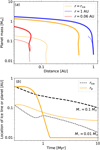 |
Fig. 6 (a) Growth tracks of protoplanets around a 0.01 M⊙ brown dwarf (thin) and a 0.1 M⊙ star (thick). The birth locations of protoplanets are at r = 0.06 AU (red), the water-ice line (orange), and r = 1 AU (blue). The protoplanets are all assumed to form at t = 0 Myr and their masses are adopted from Eq. (14) with γ = 1. In the beginning, disks are dominated by viscous heating, and rice = 0.12 AU and 0.55 AU for systems around the 0.01 M⊙ brown dwarf and 0.1 M⊙ star, respectively. (b) Time evolution of the water-ice line locations (black) and the semimajor axis of the planet (orange) for systems around stars of different masses. In these two panels the pebble-to-gas mass flux ratio is adopted to be 3%, corresponding to the stellar metallicity [Fe∕H] of 0.48. The inward movement of the ice line is faster in disks around brown dwarfs, while the migration of the protoplanets formed at the ice line is more significant around low-mass M-dwarfs. The water fraction of planets formed at the water-ice line increases with stellar mass. |
4 Population synthesis study
In this section we perform Monte Carlo simulations to study the growth and migration of a large sample of protoplanets. The initial conditions for simulated protoplanets are described in Sect. 4.1, where the distributions of model parameters are given in Table 2. We show the properties (masses, semimajor axes and water fractions) of the forming planets in the Monte Carlo sampling plots in Sect. 4.2.
Our adopted disk accretion rate follows a lognormal distribution, with the mean value given by Eq. (1) and a standard deviation σ of 0.3. The dispersion among the measured disk accretion rates onto stars of certain spectral types can be very large, ranging from 0.4 dex in Lupus (Alcalá et al. 2014)to 1 dex in Chamaeleon I star forming regions (Manara et al. 2016; Mulders et al. 2017). We note that for individual stars, the disk accretion rates also vary with time; they are high and low in early and late phases, respectively (Fig. 12 in Manara et al. 2012). The age difference among individual objects can be a few Myr even in the same star forming cluster. Therefore, the large dispersion in the accretion rate could be partially caused by this age difference. Since we already account for the time evolution of Ṁg, the standard deviation considered here should be smaller than the observed values. As in Liu et al. (2019a), we choose a standard deviation of 0.3 dex.
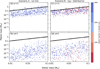 |
Fig. 7 Monte Carlo sampling plot of the planet mass as a function of the stellar mass, with the ice-line planet formation model (Scenario A) on the left, the log-uniform distributed planet formation model (Scenario B) on the right, the self-gravitating disks (γ = 1) at the top and the non-self-gravitating disks (γ ≠ 1) at the bottom. The color corresponds to the water mass fraction in the planetary core. The black line stands for a constant planet-to-star mass ratio of 3 × 10⁻⁵ motivated by Pascucci et al. (2018), which also approximates to the pebble isolation mass scaling (Lambrechts et al. 2014; Liu et al. 2019a). There is still an obvious Mp − M⋆ correlation for the central hosts in the ultra-cool dwarf mass regime of 0.01 M⊙ and 0.1 M⊙. This correlation is independent of the birth locations of protoplanets but relies on the disk conditions. Protoplanets can grow to the mass of Mars around 10MJup brown dwarfs when they are born in the self-gravitating disk phase, while they only reach 10−3 − 10−2 M⊕ when the protoplanets form later in the non-self-gravitating disk phase. Planets with ≳ 15% water can form at the water-ice line, while protoplanets formed over a wide range of disk distances end up with a distinctive bimodal water mass. |
4.1 Initial condition setup
Based on the scaling analysis from the streaming instability simulations, the masses of the protoplanets are adoptedfrom Eq. (14). The disks are assumed to be either self-gravitating (γ = 1) or non-self-gravitating (γ ≠ 1). The starting positions of these bodies are either only at the water-ice lines (Scenario A), or log-uniformly distributed from 0.01 to 10 AU (Scenario B). The formation times of these protoplanets are uniformly distributed from t = 0.1 Myr to 0.5 Myr. The masses of the central hosts M⋆ are log-uniformly adopted from the brown dwarfs of 0.01 M⊙ to the low-mass stars of 0.1 M⊙. The stellar metallicities Z⋆, corresponding to the disk pebble-to-gas mass flux ratios, range uniformly from − 0.5 to 0.5. As proposed in Sect. 2.1, the pebbles are all assumed to be 1 mm in size. Simulations are terminated at t = 10 Myr, which is the typical lifetime of gaseous disks around these ultra-cool dwarfs. We also perform simulations with t = 20 Myr and find that the final planet mass difference between two cases is less than a few percent.
4.2 Monto Carlo simulations
The resulting planet distribution obtained from our Monto Carlo simulation is illustrated in Fig. 7, which shows planet mass versus stellar mass. The masses of initial protoplanets are either obtained from the assumed self-gravitating disks (γ = 1, top), or from the non-self-gravitating, nominal two-component disks (γ ≠ 1, bottom), and their birth locations are either at the water-ice lines (left) or log-uniformly distributed over the entire disk regions (right). The black line refers to a constant planet-to-star mass ratio (Mp∕M⋆) of 3× 10⁻⁵. Based on the Kepler data, Pascucci et al. (2018) find that the most dominated planet population around GK and early M stars has such a universal planet-to-star mass ratio. Extrapolating this characteristic planet massto the stellar mass regime considered in this work, we obtain a Mars-mass planet around a 10 MJup brown dwarf and an Earth-mass planet around a 0.1 M⊙ star.
We note that the planet mass growth is limited by the black line shown in Fig. 7. Such a characteristic planet mass derived from Pascucci et al. (2018), approximately matches the pebble isolation mass, where the planet at this mass stops the inward drifting pebbles and quenches the core mass growth by pebble accretion (Lambrechts et al. 2014; Liu et al. 2019a). Therefore, irrespectively of the initial masses of the protoplanets, their final masses cannot grow beyond the pebble isolation mass. A similar conclusion has already been made in Liu et al. (2019a) where they focus on the planet formation around stars of a higher stellar mass range, from 0.1 M⊙ to 1 M⊙.
Figure 7 clearly shows that the masses of planets correlate with the masses of their (sub)stellar hosts. All planets forming around these UCDs are core-dominated with Mp ≲ 2 M⊕. This is consistent with the finding of Liu et al. (2019a) and Morales et al. (2019), where gas-dominated planets can only form in systems around stars of ≳0.2−0.3 M⊙. In the case of γ = 1 where protoplanets are born in self-gravitating disks, the planets around 10 MJup brown dwarfs can finally grow up to 0.1−0.2 M⊕. Assuming that the disk mass is 10% of the central host, such a planet mass is equivalent to ~10% of total solids in disks around these brown objects. The protoplanets around 0.1 M⊙ stars reach a maximum of≈2−3 M⊕ (Figs. 7a and c).
In the case of γ ≠ 1 where protoplanets are born in non-self-gravitating disks, we find in Figs. 7b and d that planets can ultimately reach 1 M⊕ around 0.1 M⊙ stars. However, the protoplanets around 10 MJup brown dwarfs fail to grow to Mars-mass; they only turn into planets of ~ 10−3−10−2 M⊕. There are two reasons for forming such low-mass planets around brown dwarf disks. First, the initial protoplanet-to-host mass ratio (qp = M0∕M⋆) is lower in brown dwarf disks than in M dwarf disks; for example, in the ice-line scenario M0 ~ 5 × 10⁻⁷ M⊕ around 10 MJup brown dwarfs and M0 ≃ 10−5 M⊕ around 0.1 M⊙ stars (magenta solid line in Fig. 5b). Protoplanets accrete pebbles more slowly when qp is lower (Visser & Ormel 2016). Second, disks around less massive hosts also evolve faster (Ṁg drops more rapidly, Fig. 1). Thus, the solids available for pebble accretion around brown dwarfs also drain out more quickly than around M dwarfs. Altogether, these factors limit the growth of planets above 10−2 M⊕ around 10 MJup brown dwarfs in non-self-gravitating disks.
It is worth noting that recently Miguel et al. (2020) considered planetesimal-driven planet formation model around slightly massive stars in the range of 0.05 M⊙ and 0.25 M⊙. They found that Mars-mass planets cannot form around stars of M⋆ ≲ 0.07 M⊙. For a comparison, in our model Mars-mass planets can still form in early self-gravitating disks around such low-mass brown dwarfs.
For the water-ice line scenario of r0 = rice, planets generally contain ≳15% water. We also find in Fig. 7a that planets around low-mass M dwarfs contain less water than those around brown dwarfs. Thisis because protoplanets around M dwarfs grow faster and are able to migrate inside of the ice line to accrete dry pebbles (Fig. 6b). Therefore, their final water contents become lower around such stars. As can be seen in Fig. 7b of Liu et al. (2019a), this trend also extends to the systems around solar-mass stars. However, in non-self-gravitating disks (γ ≠ 1), the initial masses of protoplanets are at least two orders of magnitude lower than those in self-gravitating disks (Fig. 5b). In this situation protoplanets grow slowly, and the inward movement of the ice line is faster than their migration, both for systems around M-dwarfs and brown dwarfs. Eventually all these planets are substantially water-rich (Fig. 7b). For the log-uniformly distributed scenario, since the ice lines are further out around more massive M-dwarfs, a higher fraction of protoplanets around such stars are born inside of the water-ice lines and finally grow into water-deficient planets. This can also be seen in Figs. 7c and d.
Figure 8 illustrates the Monte Carlo plot of the planet mass and semi-major axis. The color represents the mass of the ultra-cool dwarf. We can see that short-period planets form in the ice-line scenario, whereas planets end up with a wide range of orbital distances in the log-uniformly distributed scenario. On the other hand, we find that protoplanets around brown dwarfs are likely to grow almost in-situ, whereas a higher fraction of protoplanets around low-mass M-dwarfs grow substantially and migrate to the inner disk regions. As mentioned above, this is because the disk mass drops rapidly around brown dwarfs, and therefore the growth is marginally limited in this circumstance.
5 Conclusion
Here we present a pebble-driven population synthesis model to study how planets form around very low-mass stars and brown dwarfs in the (sub)stellar mass range of 0.01 M⊙ and 0.1 M⊙. Here we improve our model with respect to that present in Liu et al. (2019a) by (1) adopting an observed fitting formula of Ṁg (M⋆, t) from Manara et al. (2012); (2) using the stellar luminosity L⋆(M⋆, t) calculated from the advanced stellar evolution model of Baraffe et al. (2003, 2015); (3) and choosing realistic initial masses for the protoplanets based on the extrapolation of streaming instability simulations. The planet formation processes we incorporate are pebble accretion onto planetary cores, gas accretion onto their envelopes, and type I and type II planet migration (Sect. 2).
Two hypotheses on the disk conditions during planetesimal formation are explored, assuming that the disk is either self-gravitating (γ = 1) or non-self-gravitating (γ ≠ 1). Also, two scenarios for the birth locations of the protoplanets are investigated: either protoplanets form only at the water-ice line or they are log-uniformly distributed over the entire disk. We performed Monte Carlo simulations and the resulting planet population with their final planet masses, water fractions, and semi-major axes are presented in Sect. 4.
The key conclusions of this paper are listed as follows:
- 1.
Disks around low-mass stars and brown dwarfs evolve more rapidly than disks around high mass stars, as inferred from measured disk accretion rates of Manara et al. (2012). When disks are younger than 1 Myr, the disk accretion rate linearly scales with the mass of the host. However, as disks evolve over 1 Myr, Ṁg becomes gradually proportional to
 (Fig. 1).
 - 2.
We derive the characteritic mass of the planetesimals in Eq. (13) based on the extrapolation of the literature streaming instability simulations. Assuming that the protoplanets form from the planetesimal populations by streaming instability, their masses depend on both radial distances and the masses of their hosts (Eq. (14)). Protoplanets have lower masses when they are born at closer-in orbits and/or around lower-mass hosts, whereas protoplanets are more massive when they form further out and/or around higher mass hosts (Fig. 5).
- 3.
Planets formed at short orbital distances (r ≲ rice) can grow their mass substantially. However, the growth of protoplanets is very limited when they form further out (Figs. 6 and 8).
- 4.
A linearmass correlation between planets and hosts holds when protoplanets form with relative high masses in self-gravitating disks. However, this correlation breaks down when protoplanets grow in initially non-self-gravitating disks. In the latter case these protoplanets cannot reach the pebble isolation mass. Mars-mass planets can form around 0.01 M⊙ (≈10 MJup) brown dwarfs when massive protoplanets form at the early the self-gravitating phase, while protoplanets only grow up to 10−3−10−2 M⊕ when they form later in the non-self-gravitating phase. For systems around late M-dwarfs of 0.1 M⊙, the protoplanets can grow up to 2−3 M⊕. All forming planets around these ultra-cool stars are core-dominated with negligible hydrogen and helium gaseous envelopes (Fig. 7).
- 5.
Protoplanets originating at the water-ice line finally grow into water-rich planets, with ≳15% mass in water. Planets formed around higher-mass stars generally end up with lower water fractions. Water-deficient planets (
 ) can only form when protoplanets are born interior to rice
(Fig. 7).
) can only form when protoplanets are born interior to rice
(Fig. 7).
Thanks to the capabilities of current and near-future ground/ space-based planet searching programs, we are also approaching the era of discovering exoplanets around brown dwarfs. As an increasing number of planets will be detected around these tiny central objects in the coming decade, we can have fruitful data that help usbetter test and distinguish different planet formation theories.
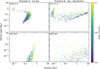 |
Fig. 8 Monte Carlo sampling plot of the final planet mass vs. the semi-major axis, with the ice line planet formation model (Scenario A) on the left, the log-uniform distributed planet formation model (Scenario B) on the right, the self-gravitating disks (γ = 1) at the top and the non-self-gravitating disks (γ ≠ 1) at the bottom. The color corresponds to the (sub)stellar mass. Scenario A only produces close-in planets, while planets formed in Scenario B have a wide range of orbital distances. Growth and migration are more significant for the protoplanets around low-mass M-dwarfs than for those around brown dwarfs. |
Acknowledgements
We thank Adam Burgasser, Thomas Ronnet, Urs Schäfer, Rixin Li and Jake Simon for useful discussions. We thank the anonymous referee for their insightful suggestions and comments. B.L. also thank TRAPPISIT-1 conference held in Liège in 2019, when many ideas of this paper are originated. B.L. is supported by the European Research Council (ERC Consolidator Grant 724687-PLANETESYS) and the Swedish Walter Gyllenberg Foundation. M.L. is funded by the Knut and Alice Wallenberg Foundation (Wallenberg Academy Fellow Grant 2017.0287). A.J. thanks the European Research Council (ERC Consolidator Grant 724687-PLANETESYS), the Knut and Alice Wallenberg Foundation (Wallenberg Academy Fellow Grant 2012.0150) and the Swedish Research Council (Project Grant 2018-04867) for research support. I.P. acknowledges support from an NSF Astronomy & Astrophysics Research Grant (ID: 1515392). T.H. acknowledges support from the European Research Council under the Horizon 2020 Framework Program via the ERC Advanced Grant Origins 832428.
Appendix A Disk model equations
Here we provide the key equations for our adopted disk model, which includes an inner viscously heated region and an outer stellar irradiation region. The detailed descriptions and derivations are referred to as Liu et al. (2019a). The gas surface density and disk aspect ratio are given by
![Mathematical equation: \begin{equation*} \frac{\Sigma_{\textrm{g}}}{\textrm{g \ cm}^{-2}} = \begin{cases} {\displaystyle 75 \left(\frac{\dot M_{\textrm{g}}}{10^{-9} M_{\odot}\,\textrm{yr}^{-1}} \right)^{1/2} \left(\frac{M_{\star}}{0.1 \ M_{\odot}} \right)^{1/8} } \\[8pt] {\displaystyle \left(\frac{r}{0.1 \ \rm AU} \right)^{-3/8} } \hfill\hspace*{9.5mm} [\mbox{vis}],\hspace*{-9.5mm} \\[.3cm] {\displaystyle 250 \left(\frac{\dot M_{\textrm{g}}}{10^{-9}\,M_{\odot}\,\textrm{yr}^{-1}} \right) \left(\frac{M_{\star}}{0.1 \ M_{\odot}} \right)^{9/14}} \\[8pt] {\displaystyle \left(\frac{L_{\star}}{0.01 \ L_{\odot}} \right)^{-2/7} \left(\frac{r}{0.1 \ \rm AU} \right)^{-15/14} } \hfill [\mbox{irr}], \end{cases}\end{equation*}](/articles/aa/full_html/2020/06/aa37720-20/aa37720-20-eq36.png) (A.1)
(A.1)
and
![Mathematical equation: \begin{equation*} h = \begin{cases} {\displaystyle 0.045 \left(\frac{\dot M_{\textrm{g}}}{10^{-9}\,M_{\odot}\,\textrm{yr}^{-1}} \right)^{1/4} \left(\frac{M_{\star}}{0.1 \ M_{\odot}} \right)^{-5/16}} \\[8pt] {\displaystyle \left(\frac{r}{0.1 \ \rm AU} \right)^{-1/16} } \hfill \hspace*{2cm} [\mbox{vis}],\hspace*{-2cm} \\[.3cm] {\displaystyle 0.0245 \left(\frac{M_{\star}}{0.1 \ M_{\odot}} \right)^{-4/7} \left(\frac{L_{\star}}{0.01 \ L_{\odot}} \right)^{1/7} }\\[8pt] {\displaystyle \left(\frac{r}{0.1 \ \rm AU} \right)^{2/7} } \hfill \hspace*{2.3cm} [\mbox{irr}],\hspace*{-2.3cm} \end{cases}\end{equation*}](/articles/aa/full_html/2020/06/aa37720-20/aa37720-20-eq37.png) (A.2)
(A.2)
where the top and bottom rows represent the quantities in the inner viscously heated region and outer stellar irradiation region, respectively, Ṁg is the disk accretion rate, M⋆, L⋆ are (sub)stellar mass and luminosity, and r is the radial distance to the central star.
The disk transition radius between these two regions is given by
 (A.3)
(A.3)
The location of the water-ice line is calculated by equating the saturated pressure and H2 O vapor pressure (Eq. (35) of Liu et al. 2019a). The water-ice line in different disk regions can be approximately given by
![Mathematical equation: \begin{equation*} \frac{r_{\textrm{ice}}}{ \ \rm AU} = \begin{cases} {\displaystyle 0.26 \left(\frac{\dot M_{\textrm{g}}}{10^{-9} \,M_{\odot}\,\textrm{yr}^{-1}} \right)^{4/9} \left(\frac{M_{\star}}{0.1 \ M_{\odot}} \right)^{1/3} } \hfill [\mbox{vis}],\\[8pt] {\displaystyle 0.075 \left(\frac{M_{\star}}{0.1 \ M_{\odot}} \right)^{-1/3} \left(\frac{L_{\star}}{0.01 \ L_{\odot}} \right)^{2/3}} \hfill\hspace*{.3cm} [\mbox{irr}].\hspace*{-.3cm} \end{cases}\end{equation*}](/articles/aa/full_html/2020/06/aa37720-20/aa37720-20-eq39.png) (A.4)
(A.4)
The ice line location is the maximum of these two values (![Mathematical equation: $r_{\textrm{ice}} \,{=}\,\max \left[r_{\textrm{ice,vis}},r_{\textrm{ice,irr}} \right]$](/articles/aa/full_html/2020/06/aa37720-20/aa37720-20-eq40.png) ).
).
Inserting Eq. (A.4) into Eq. (A.2), the disk aspect ratio at the ice line location is
![Mathematical equation: \begin{equation*} \begin{split} h_{\textrm{ice}} = \begin{cases} {\displaystyle 0.049 \left(\frac{\dot M_{\textrm{g}}}{10^{-9}\,M_{\odot}\,\textrm{yr}^{-1}} \right)^{2/9} \left(\frac{M_{\star}}{0.1 \ M_{\odot}} \right)^{-1/3}} \hfill [\mbox{vis}],\\[8pt] {\displaystyle 0.023 \left(\frac{M_{\star}}{0.1 \ M_{\odot}} \right)^{-2/3} \left(\frac{L_{\star}}{0.01 \ L_{\odot}} \right)^{1/3}} \hfill \hspace*{.3cm} [\mbox{irr]}.\hspace*{-.3cm} \end{cases} \end{split}\end{equation*}](/articles/aa/full_html/2020/06/aa37720-20/aa37720-20-eq41.png) (A.5)
(A.5)
The gas surface density at the ice line and 10 AU are also derived,
![Mathematical equation: \begin{equation*} \frac{\Sigma_{\textrm{g}}}{ \textrm{g \ cm}^{-2}} = \begin{cases} {\displaystyle 52 \left(\frac{\dot M_{\textrm{g}}}{10^{-9}\,M_{\odot}\,\textrm{yr}^{-1}} \right)^{1/3} } \hfill [{r\,{=}\,r}_{\textrm{ice}}], \vspace{0.3cm} \\ {\displaystyle 1.8 \left(\frac{\dot M_{\textrm{g}}}{10^{-9}\,M_{\odot}\,\textrm{yr}^{-1}} \right) \left(\frac{M_{\star}}{0.1 \ M_{\odot}} \right)^{9/14}} \\[8pt] {\displaystyle \left(\frac{L_{\star}}{0.01 \ L_{\odot}} \right)^{-2/7} } \hfill \hspace*{.3cm} [\mbox{\textit{r} = 10 \textrm{AU}}].\hspace*{.3cm} \end{cases}\end{equation*}](/articles/aa/full_html/2020/06/aa37720-20/aa37720-20-eq42.png) (A.6)
(A.6)
Appendix B Evolution of stellar luminosity
Stars/brown dwarfs of various masses evolve differently, and their luminosities vary with the stellar type and evolutional stage. We present an interpolation calculation of L⋆(M⋆, t) based on the stellar evolution model of Baraffe et al. (2003; below the hydrogen-burning limit) and Baraffe et al. (2015; above the hydrogen-burning limit). It is worth noting that Baraffe et al. (2015) also contains the evolutional tracks of stars and brown dwarfs with the mass range of 0.01 M⊙ and 0.1 M⊙. However, in the table provided by these latter authors, the evolution of low-mass brown dwarfs stops early, for example giving rise to 0.01 M⊙ brown dwarfs at 10 Myr. Baraffe et al. (2003) contains a longer timescale evolution for such low-mass objects. We compare the overlapping parameter space and find that the deviation of L⋆ at certain M⋆ and t from the above two studies is within 35%, which is relatively small compared to the few orders of magnitude decrease of L⋆ over time. In a future follow-up study, we plan to investigate the long-term evolution and atmosphere water-loss of these terrestrial planets. We therefore combine these two datasets together.
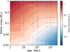 |
Fig. B.1 Stellar luminosity as function of time and stellar mass based on the stellar evolutionary model of Baraffe et al. (2003, 2015). The dots are data from the stellar evolution model, and the dashed line corresponds to the same luminosity. The black and red represent the stars above or below the hydrogen-burning limit. When the star is younger than
~ 10 Myr, |


Figure B.1 shows a full map of stellar luminosity as a function of stellar masses and time. The (sub)stellar mass ranges from 10 MJup to solar-mass. The dots represent the results from stellar evolution models, where the black and red correspond to stars in the mass range above or below the hydrogen-burning limit, i.e., M⋆ = 0.08 M⊙. As pointed out in Sect. 2.3, the stars less than ~10 Myr old show a  relation. After a few tens of millions of years, their luminosities behave as
  .
.
Appendix C Model assumption exploration
In order to test how the results in Sect. 4 vary with different model assumptions, we conduct two additional sets of simulations. Different treatments of the Ṁg−M⋆ relation and the particle size are explored in Appendices C.1 and C.2, respectively.
C.1 Different disk accretion rate-host mass correlation
In the main paper we adopt Ṁg(M⋆, t) from Manara et al. (2012). Here we choose a different Ṁg prescription from the literature. For instance, Manara et al. (2017) obtained a correlation of  (their Eq. (5)) for stars around Chamaeleon I star formation region. However, in their work there are no inferred ages of young (sub)stellar objects. Although the mean age of Chamaeleon I cluster is ~ 2 Myr, the age spreading can be as large as 2 Myr among individual objects. With no better information, we assume Ṁg ∝ t−3∕2 from the self-similar solution of the viscous accretion disk. But again, according to this setup the evolution of disks around stars/brown dwarfs of various masses is the same, which is the key difference from Manara et al. (2012). Nevertheless, from this exploration, we can learn the impact of different disk accretion and evolution conditions on planet formation. We also assume a constant Ṁg in the early embedded phase of t ≤ 0.3 Myr in order to avoid an unrealistically high accretion when t approaches 0 yr.
Compared to Fig. 1, time and host-mass dependencies on Ṁg and Md are exhibited in Fig. C.1 based on Eq. (5) of Manara et al. (2017). We find that in this case disk masses around low-mass stars and brown dwarfs are much lower than those in Fig. 1. In particular, disks around 0.01 M⊙ brown dwarfs are less than0.1% of the masses of their central hosts.
Figure C.2 shows the resulting planets from such disk conditions. Comparing Figs. C.2 and 7, we find that the final planet populations differ significantly when the disk conditions vary. Only the protoplanets close to the ice line locations in disks around hosts of ≳ 0.05 M⊙ can grow in mass and migrate to the inner disk regions. However, protoplanets seldom grow in disks around hosts of ≲ 0.05 M⊙ due to their low disk accretion rates. As expected, the building block materials provided for planet formation are much less abundant in such disks. The final planet masses and semi-major axes remain quite close to their initial values. For systems around 0.01 M⊙ brown dwarfs, planets of Mars-mass can form only at disk locations further out in self-gravitating disks. In constrastto what is shown in Fig. 7, there is no clear linear correlation between Mp and M⋆ in Fig. C.2.
Manara et al. (2017) also provided two different power-law fitting formulas for the disk accretion rate (their Eq. (4)). If this can indeed be extended to the brown dwarf mass regime, surprisingly, it indicates that very-low-mass brown dwarfs have no accretion disks (extremely low Ṁg). After forming protoplanets by streaming instability, the subsequent planet growth cannot proceed in those circumstances.
To summarize, the mechsnidm(s) by which protoplanetary disks accrete and evolve with time is a crucial condition to planet formation. Planet growth is inhibited in brown dwarf disks when accretion rates are lower than <10−13M⊙ yr−1.
C.2 Particles limited by fragmentation, bouncing and radial drift
In the main paper, we set the particles to all be 1 mm in size, which is mainly motivated by disk observations. In this section, we consider the sizes of particles from a theoretical point of view. Apart from the aforementioned bouncing barrier, dust growth also faces the radial drift and fragmentation barriers. In the dust coagulation model of Birnstiel et al. (2012), grain growth is limited by radial drift in the outer disk regions, whereas in inner disk regions fragmentation dominates. These latter authors also analytically derived the maximum stokes numbers in these two regimes.
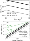 |
Fig. C.1 Panel a: time evolution of disk accretion rates among three hosts of different masses, based on Eq. (5) of Manara et al. (2017). Panel b: time and host-mass dependencies on disk mass based on Eq. (5) of Manara et al. (2017). The solid lines from thick to thin represent the ages of systems, from 0, 0.5, 1 to 3 Myr. The green dashed lines correspond to the linear, quadratic relation between the mass of the disk and that of the central host.The time evolution of the disks is the same around stars of all masses. |
The stokes number of particles in the fragmentation limit is 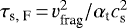 , where vfrag is the fragmentation threshold velocity, approximately 3 m/s for silicate aggregates (Blum & Münch 1993; Blum & Wurm 2008) and 10 m/s for ice aggregate (Gundlach & Blum 2015). The above equation assumes that the relative velocities of particles are lead by disk turbulence. The stokes number in the drift regime is τs, D = ɛΣpeb∕Σgη, where ɛ represents the order of unity coagulation coefficient. The surface density ratio between pebbles and gas can be calculated based on the constant flux ratio ξ assumption, which is given by
![Mathematical equation: \begin{equation*} \begin{split} \frac{\Sigma_{\textrm{peb}}}{\Sigma_{\textrm{g}}} = & \frac{\dot M_{\textrm{peb}}}{\dot M_{\textrm{g}}} \frac{u_{\textrm{g}}}{u_{\textrm{g}} + v_{\textrm{d}} } = \xi \left[ 1 + \frac{2 \tau_{\textrm{s, D}} \eta}{3 \alpha_{\textrm{g}} (1 + \tau_{\textrm{s, D}}^2) h^2} \right], \end{split} \end{equation*}](/articles/aa/full_html/2020/06/aa37720-20/aa37720-20-eq47.png) (C.1)
(C.1)
where ug and vd are the radial drift velocities for gas and dust, respectively. We assume in the bouncing limit that the particles’ size is 1 mm.
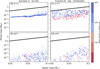 |
Fig. C.2 Monte Carlo sampling plot of the planet mass vs the stellar mass, with the ice line planet formation model (Scenario A) on the left, the log-uniform distributed planet formation model (Scenario B) on the right, the self-gravitating disks (γ = 1) at the top and the non-self-gravitating disks (γ ≠ 1) at the bottom. The initial disk conditions are followed by Eq. (5) of Manara et al. (2017). The color corresponds to the water mass fraction in the planetary core. The black line represents a constant planet-to-star mass ratio of 3 × 10⁻⁵ motivated by Pascucci et al. (2018). The planet growth is significantly suppressed compared to that shown in Fig. 7. Protoplanets cannot grow their masses in disks around brow dwarf disks of < 0.05 M⊙ due to very low disk masses. |
Figure C.3 shows the stokes numbers of particles in the radial drift (red), bouncing (black) and fragmentation (blue) limits in disks around solar-mass stars (upper), 0.1 M⊙ stars (middle) and 0.01 M⊙ brown dwarfs (lower) at t = 1 Myr, respectively. We find that the Stokes number in the bouncing limit is always lower than that in the fragmentation limit in disks around the explored central hosts. For disks around solar-mass stars, τs, B is always lower than τs, D. However, τs, B > τs, D in UCD disks when the particles are beyond a few AU. This means that millimeter-sized particles drift too quickly in these disks. As pointed out by Pinilla et al. (2013), the retention of millimeter-sized particles at a few tens of AU in brown dwarf disks is problematic.
We calculate the Stokes number to be the minimum value of the above three limits. Figure C.4 exhibits the population synthesis simulations with the updated particle sizes. When comparing Fig. C.4 and Fig. 7, we find that the planet population resulting from this model (varied particle sizes) is very similar to the model (fixed particle sizes) presented in Sect. 4. This is because, firstly, in the inner disk region of r ≲ rice, the size of pebbles is set by the bouncing barrier, meaning that there is no difference between these two models. Secondly, in the outer disk region, pebbles are in the radial drift regime with a very low Stokes number. In this case, the pebble accretion is in the inefficient 3D regime, andtherefore the protoplanets struggle to grow their masses above 10−2 M⊕ (panel d in Fig. C.4). However, for the 1 mm-sized particle model, their Stokes number soon becomes much larger than unity (Fig. 2) and pebble accretion is quickly quenched. Therefore, in that case, protoplanets are also struggle to grow large.
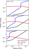 |
Fig. C.3 Stokes number of particles in the fragmentation (blue), bouncing (black) and radial drift (red) limit in 1 Myr old disks around hosts of solar-mass (upper), 0.1 M⊙ (middle) and 0.01 M⊙ (lower). The size of the particles is limited by bouncing in disks around solar-mass stars. As masses of central hosts decrease, the radial drift becomes more significant in the outer disk regions. |
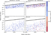 |
Fig. C.4 Monte Carlo sampling plot of planet mass vs. stellar mass, with the ice line planet formation model (Scenario A) on the left, the log-uniform distributed planet formation model (Scenario B) on the right, the self-gravitating disks (γ = 1) at the top and the non-self-gravitating disks (γ ≠ 1) at the bottom. The color corresponds to the water mass fraction in the planetary core. The black line represents a constant planet-to-star mass ratio of 3 × 10⁻⁵ motivated by Pascucci et al. (2018). Here we set the particle sizes by combined effects of radial drift, bouncing, and fragmentation. The resulting planet population is very similar to that of the fixed-sized particles model in Fig. 7. |
References
- Abod, C. P., Simon, J. B., Li, R., et al. 2019, ApJ, 883, 192 [Google Scholar]
- Ahmic, M., Jayawardhana, R., Brandeker, A., et al. 2007, ApJ, 671, 2074 [NASA ADS] [CrossRef] [Google Scholar]
- Alcalá, J. M., Natta, A., Manara, C. F., et al. 2014, A&A, 561, A2 [NASA ADS] [CrossRef] [EDP Sciences] [Google Scholar]
- Alcalá, J. M., Manara, C. F., Natta, A., et al. 2017, A&A, 600, A20 [NASA ADS] [CrossRef] [EDP Sciences] [Google Scholar]
- Andrews, S. M., Rosenfeld, K. A., Kraus, A. L., & Wilner, D. J. 2013, ApJ, 771, 129 [NASA ADS] [CrossRef] [Google Scholar]
- Ansdell, M., Williams, J. P., Manara, C. F., et al. 2017, AJ, 153, 240 [NASA ADS] [CrossRef] [EDP Sciences] [Google Scholar]
- Apai, D., Pascucci, I., Bouwman, J., et al. 2005, Science, 310, 834 [NASA ADS] [CrossRef] [PubMed] [Google Scholar]
- Bai, X.-N., & Stone, J. M. 2010, ApJ, 722, 1437 [NASA ADS] [CrossRef] [Google Scholar]
- Baraffe, I., Chabrier, G., Barman, T. S., Allard, F., & Hauschildt, P. H. 2003, A&A, 402, 701 [NASA ADS] [CrossRef] [EDP Sciences] [Google Scholar]
- Baraffe, I., Homeier, D., Allard, F., & Chabrier, G. 2015, A&A, 577, A42 [NASA ADS] [CrossRef] [EDP Sciences] [Google Scholar]
- Birnstiel, T., Klahr, H., & Ercolano, B. 2012, A&A, 539, A148 [NASA ADS] [CrossRef] [EDP Sciences] [Google Scholar]
- Bitsch, B., Morbidelli, A., Johansen, A., et al. 2018, A&A, 612, A30 [NASA ADS] [CrossRef] [EDP Sciences] [Google Scholar]
- Blum, J., & Münch, M. 1993, Icarus, 106, 151 [NASA ADS] [CrossRef] [Google Scholar]
- Blum, J., & Wurm, G. 2008, ARA&A, 46, 21 [NASA ADS] [CrossRef] [EDP Sciences] [Google Scholar]
- Burdanov, A., Delrez, L., Gillon, M., & Jehin, E. 2018, Handbook of Exoplanets (Berlin: Springer), 130 [Google Scholar]
- Burgasser, A. J., Kirkpatrick, J. D., Cruz, K. L., et al. 2006, ApJS, 166, 585 [NASA ADS] [CrossRef] [Google Scholar]
- Burrows, A., Marley, M., Hubbard, W. B., et al. 1997, ApJ, 491, 856 [NASA ADS] [CrossRef] [Google Scholar]
- Carpenter, J. M., Mamajek, E. E., Hillenbrand, L. A., & Meyer, M. R. 2006, ApJ, 651, L49 [NASA ADS] [CrossRef] [Google Scholar]
- Carrasco-González, C., Sierra, A., Flock, M., et al. 2019, ApJ, 883, 71 [NASA ADS] [CrossRef] [Google Scholar]
- Carrera, D., Johansen, A., & Davies, M. B. 2015, A&A, 579, A43 [NASA ADS] [CrossRef] [EDP Sciences] [Google Scholar]
- Chabrier, G. 2003, PASP, 115, 763 [NASA ADS] [CrossRef] [Google Scholar]
- Chabrier, G., & Baraffe, I. 1997, A&A, 327, 1039 [NASA ADS] [Google Scholar]
- Comerón, F., Neuhäuser, R., & Kaas, A. A. 2000, A&A, 359, 269 [NASA ADS] [Google Scholar]
- D’Alessio, P., Calvet, N., & Hartmann, L. 2001, ApJ, 553, 321 [NASA ADS] [CrossRef] [Google Scholar]
- Draine, B. T. 2006, ApJ, 636, 1114 [NASA ADS] [CrossRef] [Google Scholar]
- Dra̧żkowska, J., & Alibert, Y. 2017, A&A, 608, A92 [NASA ADS] [CrossRef] [EDP Sciences] [Google Scholar]
- Fontanive, C., Biller, B., Bonavita, M., & Allers, K. 2018, MNRAS, 479, 2702 [NASA ADS] [CrossRef] [Google Scholar]
- Garcia Lopez, R., Natta, A., Testi, L., & Habart, E. 2006, A&A, 459, 837 [NASA ADS] [CrossRef] [EDP Sciences] [Google Scholar]
- Gillon, M., Jehin, E., Delrez, L., et al. 2013, in Protostars and Planets VI Posters (Tucson: University of Arizona Press) [Google Scholar]
- Gillon, M., Jehin, E., Lederer, S. M., et al. 2016, Nature, 533, 221 [NASA ADS] [CrossRef] [PubMed] [Google Scholar]
- Gillon, M., Triaud, A. H. M. J., Demory, B.-O., et al. 2017, Nature, 542, 456 [NASA ADS] [CrossRef] [PubMed] [Google Scholar]
- Gundlach, B., & Blum, J. 2015, ApJ, 798, 34 [NASA ADS] [CrossRef] [Google Scholar]
- Güttler, C., Blum, J., Zsom, A., Ormel, C. W., & Dullemond, C. P. 2010, A&A, 513, A56 [NASA ADS] [CrossRef] [EDP Sciences] [Google Scholar]
- Hartmann, L., Calvet, N., Gullbring, E., & D’Alessio, P. 1998, ApJ, 495, 385 [NASA ADS] [CrossRef] [Google Scholar]
- Harvey, P. M., Henning, T., Liu, Y., et al. 2012, ApJ, 755, 67 [NASA ADS] [CrossRef] [Google Scholar]
- Herbst, W., Eislöffel, J., Mundt, R., & Scholz, A. 2007, in Protostars and Planets V, eds. B. Reipurth, D. Jewitt, & K. Keil (Tucson: University of Arizona Press), 297 [Google Scholar]
- Herczeg, G. J., Cruz, K. L., & Hillenbrand, L. A. 2009, ApJ, 696, 1589 [Google Scholar]
- Joergens, V. 2008, A&A, 492, 545 [NASA ADS] [CrossRef] [EDP Sciences] [Google Scholar]
- Johansen, A., Oishi, J. S., Mac Low, M.-M., et al. 2007, Nature, 448, 1022 [Google Scholar]
- Johansen, A., Youdin, A. N., & Lithwick, Y. 2012, A&A, 537, A125 [NASA ADS] [CrossRef] [EDP Sciences] [Google Scholar]
- Johansen, A., Mac Low, M.-M., Lacerda, P., & Bizzarro, M. 2015, Sci. Adv., 1, 1500109 [NASA ADS] [CrossRef] [Google Scholar]
- Johansen, A., Ida, S., & Brasser, R. 2019, A&A, 622, A202 [NASA ADS] [CrossRef] [EDP Sciences] [Google Scholar]
- Kirkpatrick, J. D., Gelino, C. R., Cushing, M. C., et al. 2012, ApJ, 753, 156 [NASA ADS] [CrossRef] [Google Scholar]
- Klein, R., Apai, D., Pascucci, I., Henning, T., & Waters, L. B. F. M. 2003, ApJ, 593, L57 [NASA ADS] [CrossRef] [Google Scholar]
- Kley, W., & Nelson, R. P. 2012, ARA&A, 50, 211 [NASA ADS] [CrossRef] [Google Scholar]
- Kroupa, P. 2001, MNRAS, 322, 231 [NASA ADS] [CrossRef] [Google Scholar]
- Lafrenière, D., Jayawardhana, R., Brandeker, A., Ahmic, M., & van Kerkwijk, M. H. 2008, ApJ, 683, 844 [NASA ADS] [CrossRef] [Google Scholar]
- Lambrechts, M., & Johansen, A. 2014, A&A, 572, A107 [NASA ADS] [CrossRef] [EDP Sciences] [Google Scholar]
- Lambrechts, M., Johansen, A., & Morbidelli, A. 2014, A&A, 572, A35 [NASA ADS] [CrossRef] [EDP Sciences] [Google Scholar]
- Lenz, C. T., Klahr, H., & Birnstiel, T. 2019, ApJ, 874, 36 [CrossRef] [Google Scholar]
- Li, R., Youdin, A. N., & Simon, J. B. 2019, ApJ, 885, 69 [NASA ADS] [CrossRef] [Google Scholar]
- Liu, H. B. 2019, ApJ, 877, L22 [NASA ADS] [CrossRef] [Google Scholar]
- Liu, B., & Ormel, C. W. 2018, A&A, 615, A138 [NASA ADS] [CrossRef] [EDP Sciences] [Google Scholar]
- Liu, B., Lambrechts, M., Johansen, A., & Liu, F. 2019a, A&A, 632, A7 [NASA ADS] [CrossRef] [EDP Sciences] [Google Scholar]
- Liu, B., Ormel, C. W., & Johansen, A. 2019b, A&A, 624, A114 [NASA ADS] [CrossRef] [EDP Sciences] [Google Scholar]
- Lodato, G., Scardoni, C. E., Manara, C. F., & Testi, L. 2017, MNRAS, 472, 4700 [NASA ADS] [CrossRef] [Google Scholar]
- Lynden-Bell, D., & Pringle, J. E. 1974, MNRAS, 168, 603 [NASA ADS] [CrossRef] [Google Scholar]
- Manara, C. F., Robberto, M., Da Rio, N., et al. 2012, ApJ, 755, 154 [NASA ADS] [CrossRef] [Google Scholar]
- Manara, C. F., Rosotti, G., Testi, L., et al. 2016, A&A, 591, L3 [NASA ADS] [CrossRef] [EDP Sciences] [Google Scholar]
- Manara, C. F., Testi, L., Herczeg, G. J., et al. 2017, A&A, 604, A127 [NASA ADS] [CrossRef] [EDP Sciences] [Google Scholar]
- Miguel, Y., Cridland, A., Ormel, C. W., Fortney, J. J., & Ida, S. 2020, MNRAS, 491, 1998 [NASA ADS] [Google Scholar]
- Mohanty, S., Jayawardhana, R., & Basri, G. 2005, ApJ, 626, 498 [NASA ADS] [CrossRef] [Google Scholar]
- Mohanty, S., Greaves, J., Mortlock, D., et al. 2013, ApJ, 773, 168 [NASA ADS] [CrossRef] [Google Scholar]
- Morales, J. C., Mustill, A. J., Ribas, I., et al. 2019, Science, 365, 1441 [NASA ADS] [CrossRef] [Google Scholar]
- Morbidelli, A., Lambrechts, M., Jacobson, S., & Bitsch, B. 2015, Icarus, 258, 418 [NASA ADS] [CrossRef] [Google Scholar]
- Mulders, G. D., Pascucci, I., Manara, C. F., et al. 2017, ApJ, 847, 31 [NASA ADS] [CrossRef] [Google Scholar]
- Musiolik, G., & Wurm, G. 2019, ApJ, 873, 58 [NASA ADS] [CrossRef] [Google Scholar]
- Mužić, K., Schödel, R., Scholz, A. e., et al. 2017, MNRAS, 471, 3699 [NASA ADS] [CrossRef] [Google Scholar]
- Muzerolle, J., Luhman, K. L., Briceño, C., Hartmann, L., & Calvet, N. 2005, ApJ, 625, 906 [NASA ADS] [CrossRef] [Google Scholar]
- Najita, J. R., & Bergin, E. A. 2018, ApJ, 864, 168 [Google Scholar]
- Natta, A., & Testi, L. 2001, A&A, 376, L22 [NASA ADS] [CrossRef] [EDP Sciences] [Google Scholar]
- Natta, A., Testi, L., Neri, R., Shepherd, D. S., & Wilner, D. J. 2004, A&A, 416, 179 [NASA ADS] [CrossRef] [EDP Sciences] [Google Scholar]
- Nutzman, P., & Charbonneau, D. 2008, PASP, 120, 317 [NASA ADS] [CrossRef] [Google Scholar]
- Ormel, C. W., & Klahr, H. H. 2010, A&A, 520, A43 [NASA ADS] [CrossRef] [EDP Sciences] [Google Scholar]
- Ormel, C. W., & Liu, B. 2018, A&A, 615, A178 [NASA ADS] [CrossRef] [EDP Sciences] [Google Scholar]
- Pascucci, I., Apai, D., Henning, T., & Dullemond, C. P. 2003, ApJ, 590, L111 [NASA ADS] [CrossRef] [Google Scholar]
- Pascucci, I., Testi, L., Herczeg, G. J., et al. 2016, ApJ, 831, 125 [NASA ADS] [CrossRef] [Google Scholar]
- Pascucci, I., Mulders, G. D., Gould, A., & Fernandes, R. 2018, ApJ, 856, L28 [NASA ADS] [CrossRef] [Google Scholar]
- Pérez, L. M., Chandler, C. J., Isella, A., et al. 2015, ApJ, 813, 41 [NASA ADS] [CrossRef] [Google Scholar]
- Pinilla, P., Birnstiel, T., Benisty, M., et al. 2013, A&A, 554, A95 [NASA ADS] [CrossRef] [EDP Sciences] [Google Scholar]
- Pinilla, P., Quiroga-Nuñez, L. H., Benisty, M., et al. 2017, ApJ, 846, 70 [Google Scholar]
- Przygodda, F., van Boekel, R., Àbrahàm, P., et al. 2003, A&A, 412, L43 [NASA ADS] [CrossRef] [EDP Sciences] [Google Scholar]
- Quirrenbach, A., Amado, P. J., Ribas, I., et al. 2018, Proc. SPIE Conf. Ser., 10702, 107020W [Google Scholar]
- Raghavan, D., McAlister, H. A., Henry, T. J., et al. 2010, ApJS, 190, 1 [NASA ADS] [CrossRef] [EDP Sciences] [Google Scholar]
- Reiners, A. 2012, Liv. Rev. Sol. Phys., 9, 1 [Google Scholar]
- Reiners, A., & Christensen, U. R. 2010, A&A, 522, A13 [NASA ADS] [CrossRef] [EDP Sciences] [Google Scholar]
- Riaz, B., Lodieu, N., Goodwin, S., Stamatellos, D., & Thompson, M. 2012, MNRAS, 420, 2497 [NASA ADS] [CrossRef] [Google Scholar]
- Ricci, L., Testi, L., Natta, A., et al. 2010, A&A, 512, A15 [NASA ADS] [CrossRef] [EDP Sciences] [Google Scholar]
- Ricci, L., Testi, L., Natta, A., Scholz, A., & de Gregorio-Monsalvo, I. 2012, ApJ, 761, L20 [NASA ADS] [CrossRef] [Google Scholar]
- Ricci, L., Testi, L., Natta, A., et al. 2014, ApJ, 791, 20 [NASA ADS] [CrossRef] [Google Scholar]
- Ricci, L., Rome, H., Pinilla, P., et al. 2017, ApJ, 846, 19 [CrossRef] [Google Scholar]
- Ricker, G. R., Winn, J. N., Vanderspek, R., et al. 2015, J. Astron. Telesc. Instrum. Syst., 1, 014003 [NASA ADS] [CrossRef] [Google Scholar]
- Ronnet, T., & Johansen, A. 2020, A&A, 633, A93 [CrossRef] [EDP Sciences] [Google Scholar]
- Ros, K., & Johansen, A. 2013, A&A, 552, A137 [NASA ADS] [CrossRef] [EDP Sciences] [Google Scholar]
- Schäfer, U., Yang, C.-C., & Johansen, A. 2017, A&A, 597, A69 [NASA ADS] [CrossRef] [EDP Sciences] [Google Scholar]
- Scholz, A., Jayawardhana, R., Wood, K., et al. 2007, ApJ, 660, 1517 [NASA ADS] [CrossRef] [Google Scholar]
- Schoonenberg,D., & Ormel, C. W. 2017, A&A, 602, A21 [NASA ADS] [CrossRef] [EDP Sciences] [Google Scholar]
- Shibaike, Y., Ormel, C. W., Ida, S., Okuzumi, S., & Sasaki, T. 2019, ApJ, 885, 79 [NASA ADS] [CrossRef] [Google Scholar]
- Simon, J. B., Armitage, P. J., Li, R., & Youdin, A. N. 2016, ApJ, 822, 55 [NASA ADS] [CrossRef] [Google Scholar]
- Simon, J. B., Armitage, P. J., Youdin, A. N., & Li, R. 2017, ApJ, 847, L12 [NASA ADS] [CrossRef] [Google Scholar]
- Tazzari, M., Testi, L., Ercolano, B., et al. 2016, A&A, 588, A53 [NASA ADS] [CrossRef] [EDP Sciences] [Google Scholar]
- Testi, L., Natta, A., Scholz, A., et al. 2016, A&A, 593, A111 [NASA ADS] [CrossRef] [EDP Sciences] [Google Scholar]
- Visser, R. G., & Ormel, C. W. 2016, A&A, 586, A66 [NASA ADS] [CrossRef] [EDP Sciences] [Google Scholar]
- Yang, C.-C., Johansen, A., & Carrera, D. 2017, A&A, 606, A80 [NASA ADS] [CrossRef] [EDP Sciences] [Google Scholar]
- Youdin, A. N., & Goodman, J. 2005, ApJ, 620, 459 [NASA ADS] [CrossRef] [Google Scholar]
- Zechmeister, M., Dreizler, S., Ribas, I., et al. 2019, A&A, 627, A49 [NASA ADS] [EDP Sciences] [Google Scholar]
- Zhu, Z., Zhang, S., Jiang, Y.-F., et al. 2019, ApJ, 877, L18 [NASA ADS] [CrossRef] [Google Scholar]
- Zsom, A., Ormel, C. W., Güttler, C., Blum, J., & Dullemond, C. P. 2010, A&A, 513, A57 [NASA ADS] [CrossRef] [EDP Sciences] [Google Scholar]
The above spectral index interpretation relies on the assumptions that the dust emission is optically thin and the opacity is dominated by absorption rather than scattering at the observed wavelengths (D’Alessio et al. 2001; Draine 2006; Zhu et al. 2019; Liu 2019). Recently, Carrasco-González et al. (2019) fitted the SED of HL Tau disk from ALMA and Very Large Array (VLA) data, by accounting for both scattering and absorption in dust opacity and neglecting any underlying assumption on the optical depth. From this analysis, they found that the grains have indeed already grown to millimeter sizes.
We note that, on the other hand, pebble accretion is also proposed to explain the formation of giant planet satellites (see Shibaike et al. 2019; Ronnet & Johansen 2020).
When assuming that the maximum mass and characteristic mass follow the same γ dependence, one can compare the declining trend of the orange dots and black circles in Fig. 4 to obtain a reasonable value of a.
All Tables
All Figures
|
Fig. 1 (a) Time evolution of disk accretion rates among three stars of different masses, based on Eq. (6) of Manara et al. (2012). The disk accretion rate drops faster with decreasing mass of the central object. (b) Disk mass vs. (sub)stellar mass at different times, based on Ṁg measurements of Manara et al. (2012). The solid lines from thick to thin represent the ages of systems, from 0 to 0.5, 1, and 3 Myr. The green dashed lines correspond to the linear and quadratic relation between the disk mass and the stellar mass. When the disk is ≲1 Myr old, Md ∝ M⋆, while |
| In the text | |
|
Fig. 2 Time evolution of Stokes numbers of mm-sized particles at r = rice (orange) andat r = 10 AU (blue) among three hosts of different masses. The thickness of lines represents the masses of the hosts, 1 M⊙, 0.1 M⊙, and 0.01 M⊙, respectively.The Stokes number quickly increases past unity at the distant disk location around low-mass stars, resulting in inefficientpebble accretion. |
| In the text | |
|
Fig. 3 Time and (sub)stellar mass dependencies on the luminosity of the host based on the evolutionary model of Baraffe et al. (2003, 2015). The solid lines from thick to thin indicate the systems’ ages from 1 Myr to 10 Myr, 100 Myr, and 1 Gyr. Thegreen dashed lines correspond to a linear, quadratic, cubic, and fourth power correlation between the luminosity and mass. We find that when the central host is younger than 10 Myr, |
| In the text | |
|
Fig. 4 Characteristic mass comparison among literature studies and our Eq. (12) calibrated from the results of Schäfer et al. (2017). The planetesimals obtained from streaming instability simulations are fitted by different distributions, including a single power law (dot), a simply tapered power law (triangle), a variably tapered power law (diamond), and a broken power law (square). The details of these fitting formulas are explained in the main text. The pink, orange, blue, green, and magenta refer to the studies of Johansen et al. (2015), Simon et al. (2016), Schäfer et al. (2017), Abod et al. (2019), and Li et al. (2019), respectively. We note that the orange dots only refer to the maximum masses of the planetesimals; we add the downside arrows to indicate that the characteristic masses should be lower than these values. The characteristic masses obtained in each set ofparameters are shown in symbols with the same x-axis (see Table 1). We note that Z, γ, Π, and τs are different by orders of magnitude among these numerical studies. Our Eq. (12) agrees reasonably well with the fitting characteristic masses found in these studies. |
| In the text | |
|
Fig. 5 Mass of protoplanet M0 (Eq. (14)) formed by streaming instability as a function of radial distance (left) and host mass (right). The cyan and red lines represent the protoplanets in self-gravitating disks (γ = 1) and non-self-gravitating disks (γ ≠ 1), respectively, whereas the black line corresponds to the pebble isolation mass. The birth time of the protoplanet is assumed to be at t = 0 Myr (solid) yr or 3 Myr (dashed). The mass of the central host is 0.1 M⊙ in panel a and the birth location of the protoplanet is at rice in panel b. When protoplanets form by streaming instability, their birth masses increase with both the mass of the central host and radial distance. |
| In the text | |
|
Fig. 6 (a) Growth tracks of protoplanets around a 0.01 M⊙ brown dwarf (thin) and a 0.1 M⊙ star (thick). The birth locations of protoplanets are at r = 0.06 AU (red), the water-ice line (orange), and r = 1 AU (blue). The protoplanets are all assumed to form at t = 0 Myr and their masses are adopted from Eq. (14) with γ = 1. In the beginning, disks are dominated by viscous heating, and rice = 0.12 AU and 0.55 AU for systems around the 0.01 M⊙ brown dwarf and 0.1 M⊙ star, respectively. (b) Time evolution of the water-ice line locations (black) and the semimajor axis of the planet (orange) for systems around stars of different masses. In these two panels the pebble-to-gas mass flux ratio is adopted to be 3%, corresponding to the stellar metallicity [Fe∕H] of 0.48. The inward movement of the ice line is faster in disks around brown dwarfs, while the migration of the protoplanets formed at the ice line is more significant around low-mass M-dwarfs. The water fraction of planets formed at the water-ice line increases with stellar mass. |
| In the text | |
|
Fig. 7 Monte Carlo sampling plot of the planet mass as a function of the stellar mass, with the ice-line planet formation model (Scenario A) on the left, the log-uniform distributed planet formation model (Scenario B) on the right, the self-gravitating disks (γ = 1) at the top and the non-self-gravitating disks (γ ≠ 1) at the bottom. The color corresponds to the water mass fraction in the planetary core. The black line stands for a constant planet-to-star mass ratio of 3 × 10⁻⁵ motivated by Pascucci et al. (2018), which also approximates to the pebble isolation mass scaling (Lambrechts et al. 2014; Liu et al. 2019a). There is still an obvious Mp − M⋆ correlation for the central hosts in the ultra-cool dwarf mass regime of 0.01 M⊙ and 0.1 M⊙. This correlation is independent of the birth locations of protoplanets but relies on the disk conditions. Protoplanets can grow to the mass of Mars around 10MJup brown dwarfs when they are born in the self-gravitating disk phase, while they only reach 10−3 − 10−2 M⊕ when the protoplanets form later in the non-self-gravitating disk phase. Planets with ≳ 15% water can form at the water-ice line, while protoplanets formed over a wide range of disk distances end up with a distinctive bimodal water mass. |
| In the text | |
|
Fig. 8 Monte Carlo sampling plot of the final planet mass vs. the semi-major axis, with the ice line planet formation model (Scenario A) on the left, the log-uniform distributed planet formation model (Scenario B) on the right, the self-gravitating disks (γ = 1) at the top and the non-self-gravitating disks (γ ≠ 1) at the bottom. The color corresponds to the (sub)stellar mass. Scenario A only produces close-in planets, while planets formed in Scenario B have a wide range of orbital distances. Growth and migration are more significant for the protoplanets around low-mass M-dwarfs than for those around brown dwarfs. |
| In the text | |
|
Fig. B.1 Stellar luminosity as function of time and stellar mass based on the stellar evolutionary model of Baraffe et al. (2003, 2015). The dots are data from the stellar evolution model, and the dashed line corresponds to the same luminosity. The black and red represent the stars above or below the hydrogen-burning limit. When the star is younger than
~ 10 Myr, |
| In the text | |
|
Fig. C.1 Panel a: time evolution of disk accretion rates among three hosts of different masses, based on Eq. (5) of Manara et al. (2017). Panel b: time and host-mass dependencies on disk mass based on Eq. (5) of Manara et al. (2017). The solid lines from thick to thin represent the ages of systems, from 0, 0.5, 1 to 3 Myr. The green dashed lines correspond to the linear, quadratic relation between the mass of the disk and that of the central host.The time evolution of the disks is the same around stars of all masses. |
| In the text | |
|
Fig. C.2 Monte Carlo sampling plot of the planet mass vs the stellar mass, with the ice line planet formation model (Scenario A) on the left, the log-uniform distributed planet formation model (Scenario B) on the right, the self-gravitating disks (γ = 1) at the top and the non-self-gravitating disks (γ ≠ 1) at the bottom. The initial disk conditions are followed by Eq. (5) of Manara et al. (2017). The color corresponds to the water mass fraction in the planetary core. The black line represents a constant planet-to-star mass ratio of 3 × 10⁻⁵ motivated by Pascucci et al. (2018). The planet growth is significantly suppressed compared to that shown in Fig. 7. Protoplanets cannot grow their masses in disks around brow dwarf disks of < 0.05 M⊙ due to very low disk masses. |
| In the text | |
|
Fig. C.3 Stokes number of particles in the fragmentation (blue), bouncing (black) and radial drift (red) limit in 1 Myr old disks around hosts of solar-mass (upper), 0.1 M⊙ (middle) and 0.01 M⊙ (lower). The size of the particles is limited by bouncing in disks around solar-mass stars. As masses of central hosts decrease, the radial drift becomes more significant in the outer disk regions. |
| In the text | |
|
Fig. C.4 Monte Carlo sampling plot of planet mass vs. stellar mass, with the ice line planet formation model (Scenario A) on the left, the log-uniform distributed planet formation model (Scenario B) on the right, the self-gravitating disks (γ = 1) at the top and the non-self-gravitating disks (γ ≠ 1) at the bottom. The color corresponds to the water mass fraction in the planetary core. The black line represents a constant planet-to-star mass ratio of 3 × 10⁻⁵ motivated by Pascucci et al. (2018). Here we set the particle sizes by combined effects of radial drift, bouncing, and fragmentation. The resulting planet population is very similar to that of the fixed-sized particles model in Fig. 7. |
| In the text | |
Current usage metrics show cumulative count of Article Views (full-text article views including HTML views, PDF and ePub downloads, according to the available data) and Abstracts Views on Vision4Press platform.
Data correspond to usage on the plateform after 2015. The current usage metrics is available 48-96 hours after online publication and is updated daily on week days.
Initial download of the metrics may take a while.