| Issue |
A&A
Volume 631, November 2019
|
|
|---|---|---|
| Article Number | A8 | |
| Number of page(s) | 19 | |
| Section | Stellar structure and evolution | |
| DOI | https://doi.org/10.1051/0004-6361/201935100 | |
| Published online | 11 October 2019 | |
Photometric and spectroscopic diversity of Type II supernovae
1
Department of Physics and Astronomy & Pittsburgh Particle Physics, Astrophysics, and Cosmology Center (PITT PACC), University of Pittsburgh, 3941 O’Hara Street, Pittsburgh, PA 15260, USA
e-mail: This email address is being protected from spambots. You need JavaScript enabled to view it.
2
Unidad Mixta Internacional Franco-Chilena de Astronomía (CNRS, UMI 3386), Departamento de Astronomía, Universidad de Chile, Camino El Observatorio 1515, Las Condes, Santiago, Chile
Received:
22
January
2019
Accepted:
7
August
2019
Abstract
Hydrogen-rich (Type II) supernovae (SNe) exhibit considerable photometric and spectroscopic diversity. Extending previous work that focused exclusively on photometry, we simultaneously model the multi-band light curves and optical spectra of Type II SNe using red supergiant (RSG) progenitors that are characterized by their H-rich envelope masses or the mass and extent of an enshrouding cocoon at the star’s surface. Reducing the H-rich envelope mass yields faster declining light curves, a shorter duration of the photospheric phase, and broader line profiles at early times. However, there is only a modest boost in early-time optical brightness. Increasing the mass of the circumstellar material (CSM) is more effective at boosting the early-time brightness and producing a fast-declining light curve while leaving the duration of the photospheric phase intact. It also makes the optical color bluer, delays the onset of recombination, and can severely reduce the speed of the fastest ejecta material. The early ejecta interaction with CSM is conducive to producing featureless spectra at 10−20 d and a weak or absent Hα absorption during the recombination phase. The slow decliners SNe 1999em, 2012aw, and 2004et can be explained with a 1.2 × 1051 erg explosion in a compact (∼600 R⊙) RSG star from a 15 M⊙ stellar evolution model. A small amount of CSM (<0.2 M⊙) improves the match to the SN photometry before 10 d. With more extended RSG progenitors, models predict lower ejecta kinetic energies, but the SN color stays blue for too long and the spectral line widths are too narrow. The fast decliners SNe 2013ej and 2014G may require 0.5−1.0 M⊙ of CSM, although this depends on the CSM structure. A larger boost to the luminosity (as needed for the fast decliners SNe 1979C or 1998S) requires interaction with a more spatially extended CSM, which might also be detached from the star.
Key words: radiative transfer / radiation: dynamics / supernovae: general
© ESO 2019
1. Introduction
Type II supernovae (SNe) exhibit diverse photometric and spectroscopic properties. They cover a range of brightness or luminosity (at peak or time-averaged over the high-brightness phase), visual decline rates, photospheric phase duration, and nebular phase brightness (Hamuy 2003; Anderson et al. 2014; Sanders et al. 2015). They exhibit a range of spectral line widths, absorption to emission line equivalent-width ratios (e.g., for Hα), and metal line strengths (Dessart et al. 2014; Gutiérrez et al. 2017a,b, 2018). The Hα emission and absorption strengths are correlated with the SN decline rate (Gutiérrez et al. 2017a; Chen et al. 2018). At early times, narrow emission lines are sometimes seen (e.g., Fassia et al. 2001; Smith et al. 2015; Yaron et al. 2017) whereas one expects the spectrum to form in the fastest expanding material. There is much diversity in line profile morphology (Gutiérrez et al. 2014). Polarization is also seen, sometimes to a high degree, especially at the transition to the nebular phase (see, e.g., Leonard et al. 2006, 2012).
All these features have been studied and connected to a physical model of the progenitor star and explosion. Explosion energies are expected to vary by a factor of about ten as a result of the different iron core structures in lower and higher mass red supergiant (RSG) stars (see, e.g., Ugliano et al. 2012; Sukhbold et al. 2016). This can explain the range in plateau brightness and spectral line width, as well as the nebular-phase brightness (from variations of the 56Ni yield). Progenitors with greater mass-loss rates (through stellar wind or mass exchange with a companion) will die with a smaller H-rich envelope mass, which favors a shorter photospheric-phase duration (Litvinova & Nadezhin 1985; Bartunov & Blinnikov 1992; Popov 1993). The exact outcome depends on the uncertain RSG mass-loss rates (Meynet et al. 2015) as well as the role of binarity (physics of mass exchange, frequency of binaries, etc; Yoon et al. 2010, 2017; Eldridge et al. 2018). The presence of circumstellar material (CSM) can produce excess brightness at early times (Morozova et al. 2017; Moriya et al. 2017; Dessart et al. 2017) as well as narrow lines and blue optical spectra (Groh 2014; Gräfener & Vink 2016; Dessart et al. 2016, 2017; Yaron et al. 2017). If this interaction is sustained, or if the dense shell formed from swept-up CSM is massive, it can quench the absorption and boost the emission in lines like Hα (as seen in SN 1998S; Dessart et al. 2016). Line profile diversity or polarization should also arise from asymmetry (Shapiro & Sutherland 1982), associated with a distortion of the continuum photosphere (Hoflich 1991; Jeffery 1991; Leonard et al. 2000), the presence of 56Ni “blobs” (Chugai 2006), or a combination of an asymmetric distribution of scatterers and the flux (Dessart & Hillier 2011a).
There is, however, much degeneracy in the light curves of SNe arising from RSG star explosions. The high brightness phase is mostly sensitive to the energy (kinetic and radiative) stored in the shocked H-rich envelope, while the He core material has only a small influence (Dessart & Hillier 2019a). Because stars with a very different zero age mainsequence (ZAMS) mass can have the same H-rich envelope mass at explosion, and thus similar light curves (LCs), photometric information is of little use to constrain the ejecta or the progenitor mass. The explosion energy is also hard to constrain since a significant fraction of the explosion energy is used to unbind the progenitor He core. A modest explosion in a 12 M⊙ star can produce the same ejecta kinetic energy at infinity as a powerful explosion in a 25 M⊙ star. There are also multiple combinations of energy, mass, and progenitor radius that can deliver the same Type II SN brightness (Litvinova & Nadezhin 1985). The remnant mass and envelope fallback are also poorly constrained so that the inferred ejected 56Ni mass is not a clean and direct measure of the explosive nucleosynthesis (see, e.g., Zhang et al. 2008).
To limit the impact of all these shortcomings and degeneracies, one should use all observational constraints. However, the focus is often only on light curve modeling. For example, the study of Type II SNe by Morozova et al. (2017) is based exclusively on photometric data – none of their models are tested for dynamical adequacy. In general, however, the modeling is performed using a combination of photometric data and spectroscopic data. The latter is typically limited to a single line (e.g., Fe II 5169 Å), which is used as a proxy to constrain the ejecta expansion rate. However, Fe II 5169 Å is not present prior to the recombination phase and thus provides no information on the outer, and hence fastest, ejecta material. It can also underestimate or overestimate the photospheric velocity (Dessart & Hillier 2005). The line width eventually stops decreasing during the recombination phase, no longer reflecting the recession of the photosphere toward the inner ejecta (see, e.g., Lisakov et al. 2017). Not all lines behave the same way as Fe II 5169 Å, so that a given model may reproduce well the width of some spectral lines, and overestimate or underestimate the width of others (this is particularly striking in Type II-pec SNe, whose spectra and LCs show much heterogeneity; Dessart & Hillier 2019b). The disparity in the strength and width of the absorption and emission parts of various lines (e.g., Hα) also suggests that the conditions for line formation vary significantly amongst SNe (e.g., between fast and slow decliners; Gutiérrez et al. 2017a).
In this study, we present a controlled experiment to explore the origin of the photometric and spectroscopic diversity of Type II SNe. We use two sets of progenitor models, all based on a star with solar metallicity and an initial mass of 15 M⊙. In order to generate pre-SN models with a range of envelope masses, the first set of models is produced by varying the efficiency of mass loss during the RSG phase. This variation is thought to be one mechanism for producing faster-declining light curves (Bartunov & Blinnikov 1992; Blinnikov & Bartunov 1993; Morozova et al. 2015; Moriya et al. 2016). This is the mdot model set. The second set of models, the ext set, is generated from one model in the mdot set by adding an increasing amount of CSM directly above the stellar surface. With these two model sets, we can explore the key observables produced by a reduced envelope mass or by interaction of the ejecta with a confined CSM enshrouding the progenitor star. Unlike all previous studies we assess the impact on spectra, as well as correlate the spectral and light curve properties.
In the next section, we briefly discuss the diversity of photometric and spectroscopic properties of Type II SNe, and in particular how these differ between fast (II-L) and slow (II-P) decliners. Section 3 then presents the models used in this study, including the pre-SN evolution, the treatment of the explosion, and the radiative-transfer modeling. Results from the radiation-hydrodynamics and the radiative-transfer simulations are presented in Sects. 4 and 5. The comparison to well observed slow and fast declining Type II SNe is discussed in Sect. 6, with conclusions in Sect. 7.
2. Observational diversity
2.1. Dataset
We use a few well-observed Type II SNe for comparisons and illustrations. The photometric and spectroscopic data are taken from the SN catalog (Guillochon et al. 2017) and from WISEREP (Yaron & Gal-Yam 2012). For each object, the SN characteristics (distance, reddening, redshift, explosion epoch) are adopted from the literature (Table 1). The sample includes SN 2005cs (Pastorello et al. 2009), SNe 2006qr, 2003cn, 2007oc (Anderson et al. 2014), SN 1999em (Leonard et al. 2002), SN 2012aw (Dall’Ora et al. 2014), SN 2004et (Sahu et al. 2006), SN 2013ej (Yuan et al. 2016), SN 2014G (Terreran et al. 2016), SN 1979C (Panagia et al. 1980), and SN 1998S (Fassia et al. 2000). One deviation from the literature is that we use a reddening E(B − V) = 0.3 mag rather than 0.41 mag for SN 2004et (which makes this SN more similar to SNe 1999em and 2012aw; see Sect. 6.1).
Characteristics of observed Type II SNe used in this paper.
2.2. V-band light curves of Type II SNe
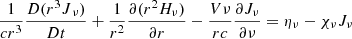
Figure 1 shows a sample of V-band light curves covering a range of rise times, brightnesses, decline rates, and photospheric phase durations. The brightest events in the set are Type IIn SN 1998S and Type II-L SN 1979C. Slightly fainter are SNe 2014G and 2013ej, which exhibit a brightness above −17 mag for about 50 days. In SN 2014G, this is followed by a short plateau and a transition to the nebular phase at about 90 d. In SN 2013ej, the light curve has a similar fading rate from the maximum, until the sudden drop at about 100 d. One step down in brightness in the group are the slow decliners or genuine plateau-like SNe II-P such as SNe 2004et, 2012aw, and 1999em. These SNe have a longer photospheric phase. Below are less luminous events, first with fast decliners (SNe 2007oc, 2003cn, and 2006qr), and finally the low-energy low-brightness Type II-P SN 2005cs. Most low-luminosity Type II SNe are slow decliners (Spiro et al. 2014; Lisakov et al. 2018).
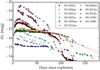 |
Fig. 1. Sample of observed V-band light curves, corrected for extinction and reddening, illustrating the well known diversity of Type II SNe (e.g., Patat et al. 1994; Pastorello et al. 2004). This diversity is representative of that shown in Anderson et al. (2014), revealing Type II SNe with a range of brightness, decline rate, and duration in their high-brightness phase. The plotting order progresses from faint to bright events at maximum (see Sect. 2.2 for discussion). |
This small set of events captures the photometric diversity of Type II SNe presented in Anderson et al. (2014), although Fig. 1 extends to higher maximum brightness (about −19.6 mag) while the larger sample of Anderson et al. (2014) peaks at −18.3 mag, with most of the events being fainter than the standard Type II-P (slow decliner) SN 1999em. In fact, SN 1999em is among the brightest Type II SNe at 100 d in the sample of Anderson et al. (2014) – only four objects are brighter in a sample of 116 objects. This seems paradoxical given that the properties of SN 1998em can be well reproduced with a standard RSG explosion model and a standard 56Ni mass (Dessart et al. 2013). Polytropic and non-evolutionary RSG progenitors have also been proposed (Utrobin 2007; Bersten et al. 2011) but this seems unnecessary. The duration of SN 1999em’s optically thick phase is also somewhat larger than average – according to Anderson et al. (2014) it is 96.0 d whereas the mean is 83.7 d1.
In some of these V-band light curves (e.g., SNe 2012aw, 2004et, 2013ej, 2014G), the rise time to a broad maximum is captured. The time of maximum is hard to measure in SN 2012aw since the curve only bends and flattens, at about 10 d. In SN 2004et, the time of maximum is around 20 d. For the brighter events, SNe 2013ej and 2014G, the time of maximum is slightly greater than 10 d. Overall, these values are larger than those of González-Gaitán et al. (2015), who report a median rise time of 7.5 d in the rest-frame g′-band (λ4722) from their sample of 223 events (but there is considerable dispersion, and some rise times approach 20 days). Their study was based on the Sloan Digital Sky Survey (SDSS) – II Supernova Survey (Sako et al. 2014) and the Supernova Legacy Survey (Guy et al. 2010). The distributions of rise times from the two surveys were somewhat different, and this was attributed to the better cadence of the SDSS data. González-Gaitán et al. (2015) also concluded that the radii of the SN progenitors are, on average, smaller than those of known RSGs.
The rise times for a sample of 20 core-collapse SNe with both well-constrained explosion times and light curves have been provided by Gall et al. (2015) who find mean rise times of 7.0 ± 0.3 d for II-P SNe and 13.3 ± 0.6 d for Type II-L SNe. However, they note that the rise time of the Type II-L SNe might be biased upward by the most luminous events which tend to have the most well-defined explosion times. Their study also found that larger progenitor radii and higher explosion energies lead to a larger peak brightness at optical wavelengths.
These V-band rise times are however shorter than expected for the explosion of a RSG star. Dessart & Hillier (2011b) presented the first non-LTE time-dependent radiative-transfer modeling of RSG star explosions which allowed for the detailed influence of lines and in particular line blanketing. They reported that for a standard RSG star progenitor of 15 M⊙ initially, the resulting Type II SN light curve exhibits a rough plateau morphology but with a long rise time of ∼50 d in the V-band. This rise time is associated with the delay until the onset of hydrogen recombination since this signals the time when the photospheric temperature is around 5000−7000 K and the spectral energy distribution peaks in the V-band. The only way for such a model to produce a shorter rise time is to produce a more rapid recombination, analogous to what is seen in events like SN 1987A (whose photosphere recombines after just a few days). In other words, this rise time is controlled by a color shift from the UV to the optical. Using a more compact RSG progenitor (reduced from 810 to 500 R⊙), the Type II-P SN light curve of model m15mlt3 peaks earlier to a flat maximum, at around 20−30 d (Dessart et al. 2013). Importantly, there is no longer a color offset between the observations of SN 1999em and the model m15mlt3.
The Type II SN rise time of 7.5 d reported by González-Gaitán et al. (2015) is incompatible with the modeling results discussed above. Such a short rise time cannot result from the spectral energy distribution shift to optical bands as the ejecta cools and recombines because RSG stars are too big to allow for this. An alternative is that the short rise time is associated with a bolometric boost resulting from interaction with confined CSM at the surface of the RSG progenitor. The early-time observations of SN 2013fs provide empirical evidence for this (Yaron et al. 2017). It now seems that such a CSM is a fundamental feature of RSG stars and may impact, at various levels, all Type II SNe (Yaron et al. 2017; Morozova et al. 2017; Dessart et al. 2017; Moriya et al. 2017; Förster et al. 2018). However, since the majority of events in Anderson et al. (2014) are fainter than SN 1999em, the interaction with CSM (which produces a luminosity boost) cannot be the only driver for Type II SN diversity. Neither can it explain the scatter in photospheric-phase duration.
2.3. Observed properties of Hα profiles in Type II SNe
The luminous fast decliners SNe 2013ej, 2014G, 1979C and 1998S (in order of increasing early-time brightness) show drastically different spectral properties in the Hα region both at 15 and 60 d after explosion compared to the more standard Type II-P (i.e., slow decliners) SNe 2005cs, 2012aw, 1999em, and 2004et (Fig. 2). At both epochs, standard Type II-P SNe show a well-developed P-Cygni profile. At 15 d (hence close to the time of V-band maximum), the Hα profile has a broad absorption and a strong emission (the two leftmost columns). Both absorption and emission are Doppler broadened. The absorption is weaker and broader so it is difficult to assess the maximum velocity in the line. Si II 6355 Å contributes to the absorption and extends it. The maximum velocity attributed to Hα seems however quite large, and probably in the range 10 000−15 000 km s−1 for SNe 1999em, 2012aw, and 2004et (it is less than 10 000 km s−1 in SN 2005cs, whose slower expansion rate makes the contribution of the Si II line clearly visible). At 50 d (i.e., during the recombination phase), the Hα line profile is stronger and still very broad, but the absorption does not extend beyond about 10 000 km s−1. This implies that the outer ejecta of these II-P SNe are sufficiently dense to maintain Hα optically thick at 10 000 km s−1; it also implies that there is material accelerated to such large velocities (something that a massive CSM may prevent).
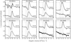 |
Fig. 2. Comparison of spectra in the Hα region at about 15 and 60 d after the inferred time of explosion for a set of observed Type II SNe with a range of V-band decline rates during the photospheric phase. The spectra have been normalized so that the peak value (in the spectral window shown) is unity, with an additional offset of unity for the upper spectrum. Left-most two columns: standard Type II SNe with a slow decline rate. Third column: SNe that exhibit a much larger brightness at early times followed by a fast decline. Rightmost column: SNe with a huge early-time brightness and a fast decline rate at all times. The photometric differences between these families of events have a clear spectroscopic counterpart (see Sect. 2.3 for discussion). |
In SN 2013ej, the Hα profile at 13.5 d shows stronger absorption from Si II and weaker absorption from Hα, while the Hα line emission strength is reduced. However, at 50.5 d, it looks similar to the standard SNe II-P previously discussed. In contrast, in SN 2014G, the Hα region at 16.4 d is essentially featureless. Two blue-shifted absorptions (probably associated with Hα and Si II 6355 Å) without emission are now seen, while the Hα profile at 52.4 d is clearly present, but with a weak absorption relative to standard SNe II-P. This absorption is also less extended in velocity space.
The rightmost column in Fig. 2 shows the properties for SNe 1979C and 1998S, which are analogous to those discussed for SN 2014G but more extreme. The Hα region at about 15 d is almost featureless while at 70 d the Hα profile shows no absorption component, even though the emission line strength at this epoch is similar to the other SNe.
SN 1998S has been modeled by Dessart et al. (2016), who find that the interaction of a standard RSG explosion with 0.4 M⊙ of CSM at 1015 cm reproduces both the light curve and the spectral evolution. This evolution includes the presence of narrow lines early on (at that time, the spectrum forms in unshocked ionized slow-moving CSM), followed by a blue featureless spectrum with blueshifted absorptions (the spectrum forms in the dense shell formed by the swept-up CSM), and finally a more typical SN II spectrum but with weak signs of blanketing and a strong Hα emission with no associated absorption.
It thus appears that the spectral properties shown in Fig. 2 correspond to a continuum of events in which the mass of CSM grows from small to significant (from left to right). This interpretation agrees with the photometric properties discussed in Sect. 2.2. While the photometry can help constrain the amount of CSM, the spectral information can help constrain the impact of the CSM on the ejecta dynamics, as we discuss below.
3. Numerical setup
The numerical approach used for this study is similar to our previous work on Type II SNe with and without CSM (see, e.g., Dessart et al. 2013, 2017). It involves stellar evolution calculations with MESA (Paxton et al. 2011, 2013), radiation hydrodynamics simulations of the explosion with V1D (Livne 1993; Dessart et al. 2010a,b), and non-LTE time-dependent radiative transfer simulations with CMFGEN (Hillier & Dessart 2012).
All simulations presented here are based on a star with solar metallicity and an initial mass of 15 M⊙. The evolution, until the onset of core collapse, is performed with MESA version 4670 using the default parameters and the modifications specified in Dessart et al. (2013). An old MESA version was used because all MESA simulations were performed in Feb. 2013, when this project was started. The mixing length parameter αMLT was changed from 1.6 to 3. This was necessary to produce more compact RSG stars at the time of explosion, since very extended RSG stars produce SNe II-P with a delayed recombination, in conflict with observations (Dessart et al. 2013).
For the mdot model set (we label the models as xval where val is the mass loss rate scaling factor), the mass-loss rate was scaled by a factor 1.5, 2.0, 3.0, 4.0, 5.0, 6.0, 7.0, 8.0, 9.0, and 10.0 when the model effective temperature dropped below 4000 K. Hence the scaling only applies during the RSG phase; the higher effective temperature of these RSG star models implies that by default their mass-loss rates would be lower than for standard RSG star models computed with a lower mixing length parameter. The scaling of the mass-loss rates yields pre-SN progenitors with similar surface radii (from about 580 to 680 R⊙), similar He core masses (from 3.99 to 4.27 M⊙), but different H-rich envelope masses (from 0.91 to 9.48 M⊙).
The ext model set is generated from the pre-SN model x3p0 by adding an atmosphere with a density scale height that varies from 0.05 (model x3p0ext1) to 1.0 R⋆ (model x3p0ext6) and extending out to a radius where the density drops to 10−12 g cm−3. One additional model (x1p5ext3) was done based on model x1p5 because it was found to be well suited for SN 2012aw. The corresponding mass of this CSM increases from 0.022 (model x3p0ext1) to 1.973 M⊙ (model x3p0ext6). Figure 3 illustrates the density structure, versus Lagrangian mass and radius, for these two model sets. Table 2 summarizes the main model properties. In that table MH, e is the envelope mass defined as the mass above a hydrogen mass fraction of ∼0.3, while MHe, c is the core mass, and is simply Mf − MH, e where Mf is the progenitor mass at core collapse.
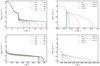 |
Fig. 3. Left: mass density versus Lagrangian mass (top) and radius (bottom) at the onset of core collapse for the set of 15 M⊙ simulations produced with MESA using a mixing-length parameter of 3 and a variety of mass-loss rate scalings during the RSG phase. Right: same as left, but now for variants of model x3p0 in which some CSM has been added. The corresponding model properties are given in Table 2. |
Summary of progenitor and ejecta properties.
The surface radius of RSG progenitors is a fundamental parameter that impacts both the brightness (see, e.g., Litvinova & Nadezhin 1985) and color evolution (Dessart et al. 2013) of Type II SNe. Recently, Paxton et al. (2018) studied Type II SNe and used a mixing-length parameter of 3 for the progenitor evolution, as here and in Dessart et al. (2013). In contrast, Morozova et al. (2017) took the massive star models of Woosley & Heger (2007), which are computed with a lower mixing-length parameter. As a consequence, their model set of 12−30 M⊙ progenitors collapse as RSG stars with a surface radius between 640 (12 M⊙) and 1550 R⊙ (30 M⊙). Their 15 M⊙ model has a surface radius about 30% larger than those in our mdot set. Such large radii are in tension with the color evolution of SNe II-P but may be possible in events where the SN radiation stems predominantly from interaction (and thus do not look like SNe II-P).
In addition to issues with the radii of SN progenitors, there are significant issues with the structure of RSG photospheres, mass-loss rates, and the immediate CS environment. Betelgeuse is the nearest RSG and has been the subject of numerous studies. Its atmosphere is extended over a few stellar radii, shows a non-monotonic temperature structure, inhomogeneities, large convection cells, and strong asymmetries (e.g., O’Gorman et al. 2017). Betelgeuse also has a shell of atomic hydrogen at a distance of 0.24 pc from the star (Le Bertre et al. 2012). From the properties of this shell it is inferred that Betelgeuse has been losing mass at a rate of 1.2 × 10⁻⁶ M⊙ yr−1 for about 8 × 10⁴ yr (Le Bertre et al. 2012). Mackey et al. (2014) argue that the shell is maintained by pressure from the photoionized wind which is ionized by external sources. A recent review of high spatial resolution observations of RSGs is by Ohnaka (2017).
It is also unclear whether the CSM when the RSG explodes is similar to that found earlier in its evolution. Changes in global properties of the star (over the final 10 000 years) will potentially lead to large changes in mass loss and pulsation characteristics, thus affecting the photosphere and CSM (Heger et al. 1997). Heger et al. (1997) also postulate that a superwind may occur prior to collapse. However archival studies of several SN progenitor sites by Johnson et al. (2018) indicate that the magnitudes for the RSG progenitors of four SNe were stable to within 10%.
Each model in the mdot and ext sets is exploded by means of a piston, placed at a Lagrangian mass of 1.6 M⊙, to deliver an asymptotic ejecta kinetic energy of 1.2 × 1051 erg. Because the models have a slightly different core structure, the explosion produces different 56Ni masses, from 0.007 up to 0.056 M⊙. When these models were computed in 2013, no attempt was made to correct for this. Because the focus of our study is on the diversity of Type II SN light curves during the high brightness phase, the 56Ni mass was left as it was and the resulting ejecta models have, consequently, a different brightness at the end of the photospheric phase and beyond2.
At 10−15 d after the piston trigger, the V1D simulations are remapped into CMFGEN. Homology is enforced, which causes a small adjustment to the 56Ni mass, and the SN age is set to R/V. The models in the mdot (ext) set were exploded with V1D in 2013 (2018) and a different approach for mixing was used in each set. For the mdot set, a boxcar algorithm is used to mix the composition. The resulting mixing is weak. In the ext set, we make the material within 5 M⊙ both homogenous and of constant density, and then operate a Gaussian smoothing on both the density and the composition. As a consequence, the H mass fraction in the innermost ejecta varies from ∼0.1 in model x1p5 to almost 0 in model x1e1, but it is 0.3 in all the ext models. One reason for doing this is that physically, the reverse shock should lead to a smearing of the H/He interface in the ejecta and a strong mixing of the He core material with the base of the H-rich envelope (Paxton et al. 2018; Utrobin et al. 2017). A density profile with strong gradients can lead to problems with mass conservation across a time sequence computed with CMFGEN; as noted above, such strong gradients are an artifact of 1D).
The CMFGEN models are evolved until 200–300 d after explosion. The model atoms are similar to those of Dessart et al. (2013). The γ-ray energy deposition is computed using a gray pure-absorption radiative transfer solver and a depth-dependent opacity of 0.06Ye cm2 g−1 (where Ye is the electron fraction). Non-thermal processes are treated as in Li et al. (2012). In CMFGEN, the ejecta is assumed to expand freely in a vacuum. There is thus no ongoing interaction considered, for example, with the progenitor RSG wind material. A comparison of the CMFGEN light curves with those of V1D (Fig. B.1) for the x3p0 model set, together with a discussion on the causes of the (relatively small) differences is provided in Appendix B. Figure B.1 also illustrates the influence of the different CSM structures on the light curve for the x3p0 model set. We illustrate the temporal evolution of the temperature for two of the models (x3p0 and x3poext4) in Fig. C.1.
By starting at 10−15 d after explosion, the CMFGEN simulations miss the earlier evolution. This is not a major problem. Studies dedicated to the earlier, dynamical, evolution can be done using a different technique (Dessart et al. 2017). As such, the present CMFGEN simulations are complementary. Observations at the earliest times are also rare. Early interaction with CSM, for example, leaves an imprint on the ejecta that is visible for weeks after explosion. So, the current modeling with CMFGEN is not strongly affected by this shortcoming. We also note that numerous studies focus exclusively on light curve modeling, and thus are unable to constrain the complexity of the CSM interaction, whose information is contained in the spectra that these studies ignore.
These CMFGEN simulations use a slightly improved numerical procedure (in place since 2015) to improve energy conservation in time. In particular, the transfer equations to be solved are now written in the form
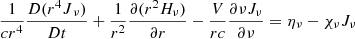 (1)
(1)
rather than
 (2)
(2)
with a similar modification for the flux equation. This modification leads to improved energy conservation during the photospheric phase. The meaning of the symbols is the same as in Hillier & Dessart (2012), with the exception of the velocity, for which we use the symbol V rather than v to avoid confusion with the frequency ν. The procedure used to examine the energy conservation in time is described in Appendix A.
4. Results from radiation hydrodynamics simulations
We first discuss the results from the radiation hydrodynamics simulations. Figure 4 shows the bolometric luminosity (top), the photospheric velocity (middle), and the photospheric temperature (bottom) for both model sets.
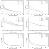 |
Fig. 4. Left: evolution of the bolometric luminosity (top), the photospheric velocity (middle), and the photospheric temperature (bottom) for the explosion models computed by V1D and based on the mdot model set. Right: same as left, but now for the ext model set (see Sect. 4 for discussion). |
If the ejecta mass is reduced for a fixed ejecta kinetic energy (mdot set; left column), the bolometric light curves progressively shift to a faster decline and an earlier transition to the nebular phase, as expected (Blinnikov & Bartunov 1993; Morozova et al. 2015; Moriya et al. 2016). The larger Ekin/Mej implies larger photospheric velocities early on, but since the ejecta optical depth is lower, the photosphere reaches the slower inner ejecta earlier. This causes a faster decline of the photospheric velocity. However, all models show the same evolution for the photospheric temperature evolution. The temperature for H recombination (i.e., around 7000 K) is reached after about 20 d. The principal cause for the variation in the light curves is the variation in MH, e – there is a direct effect due to the lower envelope mass and an indirect effect arising from more rapid expansion of the envelope.
For a fixed ejecta mass and kinetic energy (corresponding to those of model x3p0), an increasing amount of CSM (ext set; right column) causes a stronger and longer-lived boost to the luminosity. For a CSM of about 0.2 M⊙ (model x3p0ext3), the boost is limited to times prior to 20 d, but for the highest CSM mass of about 2 M⊙ (model x3p0ext6), nearly the entire photospheric phase is affected. The photospheric phase duration is in general not affected by the presence of CSM, except in model x3p0ext6 in which the reverse shock (caused by the CSM) reached down to the inner ejecta layers, slowing it down and depositing additional internal energy. The boost in luminosity arises here from interaction, converting kinetic energy to radiation energy. The luminosity boost is thus associated with a reduction of the outer ejecta kinetic energy and maximum velocity. The evolution of the photospheric velocity is a quasi-monotonic decrease from 12 000 to 5000 km s−1 in model x3p0 (no CSM) but is instead a plateau at 5000 km s−1 for the first 40 d in model x3p0ext6.
In the ext models, the reduced maximum velocities are not only a result of braking arising from interaction with the CSM. This certainly occurs, but unlike in SNe ejecta interacting at large distances, the interaction takes place here when the shock reaches the stellar surface. At that time, about half the total energy is radiation, and the other half is kinetic. By interacting with CSM at a moderate optical depth, a sizable fraction of the shock energy is lost to escaping radiation. If the configuration was adiabatic (i.e., no radiative losses), the kinetic energy would first drop and be converted into radiation energy. Then, this radiation energy would be tapped to accelerate the ejecta again. This second step does not happen fully here because of radiation leakage, which causes the boost to the emergent luminosity.
The hydrodynamics of the SN shock interacting with a variety of CSM structures, and the effect of interactions on the SN photometric and spectroscopic properties during the first 15 d after shock breakout, have been discussed in Dessart et al. (2017). Additional details that can be found there are not repeated here.
In the ext models, the evolution of the photospheric temperature is qualitatively similar between models, but quantitatively, the greater the CSM mass, the greater the photospheric temperature. This arises from the excess energy dissipated in the outer progenitor layers during the interaction. Because this takes place at the largest possible radii in the star, this energy is not strongly degraded by expansion. In contrast to the mdot models, we expect a color shift of the SN radiation in the ext models, associated with a delayed recombination.
Overall, both the mdot and ext model sets tend to produce more linearly declining bolometric light curves as the H-rich envelope mass is reduced or the CSM mass is enhanced. However, the boost in luminosity is large and sustained only for the ext case. This is not surprising since interaction gives an efficient means to extract energy from where it is the most abundant (i.e., the ejecta kinetic energy).
In nature, fast decliners may stem from these two scenarios (and perhaps others, not yet identified). But from Fig. 4, the two above scenarios for the production of fast declining Type II SNe can be easily distinguished. If fast decliners primarily arise from a reduction of the progenitor H-rich envelope mass, the maximum ejecta velocities in II-L should be larger, the photospheric phase shorter, and the color similar to Type II-P. If fast decliners instead arise from interaction with CSM, the maximum ejecta velocities of II-L should be smaller, the photospheric velocity evolution should be flatter, the photospheric phase should have (statistically) the same duration as Type II-P, and the color should be bluer for longer compared to Type II-P SNe. Furthermore, this configuration would produce SNe that may appear as Type IIn at early times. The two scenarios may occur simultaneously, so that fast decliners may come from progenitors with a reduced H-rich envelope mass and enshrouded within a massive and confined CSM. For example, the greater mass-loss rates in higher mass progenitors may lead to both a greater CSM mass and a reduced H-rich envelope mass. Such a correlation could be expected from stellar evolution theory.
5. Results from non-LTE time-dependent radiative transfer simulations
Figure 5 shows some of the results from the CMFGEN simulations based on the mdot and the ext simulations undertaken with V1D and MESA. This figure is a counterpart of Fig. 4, with mdot models on the left and ext models on the right, but now showing the absolute V-band light curves (which reflect in part the bolometric light curve, modulo the change in V-band bolometric correction), the Hα profile in velocity space (which reflects the behavior in photospheric velocity), and the color evolution (which reflects the evolution of the photospheric temperature). We also add photometric observations for comparison, including slow (SN 1999em) and fast decliners (same SNe as shown in Fig. 1).
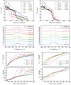 |
Fig. 5. Left: illustration of the absolute V-band light curves (top), the spectral region centered on Hα at about 20 d after explosion (middle), and the U − V and V − I color curves (bottom) for the mdot simulations performed with CMFGEN. Right: same as left, but now for the ext model set (see Sect. 5 for discussion). |
In the mdot model set, reducing the H-rich envelope mass leads to a <1 mag increase in V-band brightness at 15 d, while it causes a progressive shortening of the high brightness phase. The shorter the photospheric phase, the faster the decline, so that the brightness becomes smaller than standard Type II-P SNe earlier (taking SN 1999em as representative). Increasing the kinetic energy would raise the luminosity at early times but the decline would be even faster. As seen in the properties of the photospheric velocity (middle left panel of Fig. 4), the models with lower H-rich envelope mass exhibit a broader Hα profile at 20 d after explosion. Reflecting the similar photospheric temperature evolution, the color evolution for the mdot set is similar during the photospheric phase. The optical colors redden and diverge between models when the ejecta turns optically thin.
In the ext set, the presence of CSM reduces the rise time in the V-band so that in model x3p0ext3, the V-band light curve is essentially flat at and beyond 10 d. Increasing the CSM mass yields an increase in V-band brightness that spans between the values for SN 1999em and SN 2014G. SNe 1979C and 1998S require either more CSM mass or a different configuration. This could be an interaction at larger distances (Dessart et al. 2016), or a sustained interaction with a dense pre-SN wind over very large distances (Blinnikov & Bartunov 1993). Around 1 M⊙ of CSM seems necessary to explain the early-time V-band brightness of SNe 2013ej and 2014G. This depends on both the mass of CSM and its spatial distribution. It also depends on the V-band bolometric correction, which can be hard to estimate accurately since a significant fraction of the flux falls in the UV at early times.
As expected from Fig. 4, the lower velocities in the outer ejecta in the ext models strongly impact the Hα profile at 20 d (the interaction is over by then). As the CSM mass increases, the Hα profile becomes weaker in both absorption and emission. The absorption component vanishes in models x3p0ext5 and x3p0ext6, while only a residual emission subsists in model x3p0ext6. The enhanced CSM mass also causes the optical color to be bluer (the spectrum formation region is hotter for longer).
The primary reason for the weakness of the Hα profile at early times is that in these models the photosphere is located in a dense shell formed from the interaction of the ejecta with the CSM. As this shell is moving at near constant velocity and because the density profile is very steep, the P Cgyni profile is weak or absent. At later times the P Cgyni absorption is weak or absent primarily because of the absence of high velocity material. For SN 2006bp we reproduced the weakness of Hα using a steep density profile (ρ ∝ r−50; Dessart et al. 2008). The same effect is inferred for SN 1998S, although in this case the interaction of the ejecta with a massive CSM is thought to have occurred at large distances (Dessart et al. 2016). Finally, the influence of the CSM on the SN radiation is extensively discussed and explained in Dessart et al. (2017), to which the reader is referred.
To summarize, a fast decline with the mdot model set inevitably leads to a short photospheric phase duration. Reducing the H-rich envelope mass is not conducive to producing a strong boost to the early-time brightness. This modest boost in brightness is correlated with the Hα line width (i.e., brighter, broader) while the color during the photospheric phase is independent of the brightness boost.
With the ext model set, the boost in V-band brightness is larger, compatible with the observations of SN 2013ej and 2014G, but too small to reach that seen for SN 1979C and SN 1998S. The boost in luminosity is anti-correlated with the width of Hα, which may also appear as pure emission early-on (Type IIn features may be seen at earlier times; Dessart et al. 2017). The color also correlates with the brightness boost in that the greater the boost, the bluer the color, and the more delayed is the onset to recombination.
Figures 6 and 7 illustrate the differences in the Hα line region between ∼15 and ∼50 d after explosion, as shown earlier for a sample of Type II SNe with a range of V-band brightnesses and decline rates (Fig. 2). The mdot models show the same evolution as that seen in standard slow decliners: the Hα profile is a well developed P-Cygni profile at both epochs and its width narrows in time (the extent of the absorption part is also affected by Si II 6355 Å at 15 d). In the ext model set, the contrast between models is strong. As the CSM mass is enhanced from model x3p0 to x3pext6, we see that Hα progressively shows a weaker absorption and emission at 15 d. At 50 d, the line shows a weaker absorption, but the emission remains strong and broad.
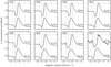 |
Fig. 6. Comparison of spectra in the Hα region at about 15 and 50 d after explosion for the model set with decreasing H-rich envelope mass (from x1p5 to x1e1). |
The trend seen from left to right in Fig. 7 is analogous to that displayed in Fig. 2 (the CSM mass increases as we progress from slow to (luminous) fast decliners). Another feature of interest is the presence of a high-velocity notch in the Hα absorption in model x3p0ext2 at 50 d. Such a notch is observed in numerous Type II SNe (Gutiérrez et al. 2017b) and has been associated with the dense shell that forms out of the swept-up RSG wind material (Chugai et al. 2007). Here, the process is similar except that the dense swept-up shell is associated with the CSM originally around R⋆. In models with less CSM, the dense shell is not dense enough. In models with more CSM, the dense shell moves more slowly. In model x3p0ext3, its associated absorption merges with the absorption from lower velocities so no notch is visible. The same applies to model x3p0ext5 but the absorption is now filled in by emission from the dense shell. In model x3p0ext6, the shell speed is even lower, its density higher, and the absorption vanishes. It may be that in Nature, the high-velocity notch observed in Hα comes primarily from swept-up CSM during the first few days after shock breakout.
6. Comparison to observations
It is beyond the scope of this study to make a comparison to a large sample of Type II SNe. Instead, this section presents a comparison of a few models from the mdot and ext sets to a few representative SNe exhibiting different V-band decline rates. Unlike all previous studies, we compare both multi-band light curves and multi-epoch optical spectra.
To avoid confusion, let us stress again that this section presents comparisons and not fits to observations. To produce a good fit to observations, a large number of simulations are performed, and the model that produces the best χ2 is selected. As we have produced only a handful of models with sizable differences between them, a good “fit” to data would be largely incidental. Our models are therefore presented as comparisons in this section. When evaluating the offset between the model and the data, the reader is asked to evaluate whether a simple change in parameters could resolve the offset. The documented dependences between ejecta and progenitor properties on the one hand, and the observables on the other can be used to do this. For example, a change of 1 M⊙ in ejecta mass lengthens the plateau duration by 10 d in the low-energy model X for SN 2008bk (Lisakov et al. 2017).
6.1. Comparison to slow decliners
6.1.1. SN 1999em
SN 1999em has been extensively studied. It was the first Type II-P SN detected at both radio and X-ray wavelengths (Pooley et al. 2002). Pooley et al. (2002) argue that the X-ray observations indicate a pre-SN wind with a mass-loss rate of approximately 2 × 10⁻⁶ M⊙ yr−1 and a speed of 10 km s−1. Extensive photometric and spectroscopic observations have been discussed by Elmhamdi et al. (2003) who indicate that dust formed after day 465. Several studies of SN 1999em have used the “expanding photosphere method” (EPM; Hamuy et al. 2001; Leonard et al. 2002), or a variant, to determine its distance (Baron et al. 2004; Dessart & Hillier 2006). The last two studies derived distance estimates more consistent with that obtained using cepheids.
Figure 8 presents a comparison of model x2p0 (mdot set, no CSM) with the observations of SN 1999em, including the UBVRI light curves (top) and the multi-epoch spectra from 10.9 d until 168.6 d after the inferred time of explosion. The model qualitatively reproduces the photometric and spectroscopic data, from the early photospheric phase until well into the nebular phase. The multi-band light curves are well matched in all bands. The slight underestimate of the optical brightness at 10 d suggests that a small amount of CSM would help.
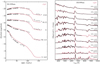 |
Fig. 8. Comparison of multi-band light curves (left) and multi-epoch spectra (right) for SN 1999em and model x2p0. The time origin is the inferred time of explosion. For the spectral comparison, the model is redshifted and reddened, and the label ΔMV gives the V-band magnitude offset at each epoch. The spectra are normalized to each other and shifted for better visibility. |
Matching the transition to the nebular phase better merely requires a slight adjustment to the H-rich envelope mass, the explosion energy, and the 56Ni mass. Here, the model x2p0 reproduces roughly this transition (it occurs about 10 d too early). The nebular-phase brightness is underestimated by about 20% (it depends on the filter considered), so an increase of the 56Ni mass from 0.036 to about 0.043 M⊙ would reduce the offset at nebular times and also lengthen the plateau (and thus reduce the offset mentioned earlier).
Taken individually, some lines show slight offsets. For example, Na I D strengthens more slowly than observed, the Hα absorption is a little too broad (but the width of the emission is well matched), and Hβ disappears in the observations during the second part of the plateau but is always present in the model. Some discrepancies emerge at late times, such as the overestimate of the emission strength of He I 7065 Å. All these offsets are worth further investigation but they are small and do not alter the conclusions that can be drawn from the comparison. Importantly, we have shown that the model qualitatively, and to a lesser extent, quantitatively, matches simultaneously the multi-band light curves and spectra of SN 1999em. In other words, a 15 M⊙ progenitor model exploding with an H-rich envelope mass of about 9 M⊙, and producing an ejecta with about 1.2 × 1051 erg kinetic energy and 0.036 M⊙ of 56Ni is broadly compatible with observations. A small contribution from CSM would improve the match before 15 d (see next section on SN 2012aw), and a 20% greater 56Ni mass would improve the agreement after 100 d.
The model of Utrobin (2007) for SN 1999em is similar to model x2p0 except that the ejecta mass is 19 M⊙ and the progenitor density structure is crafted. Using a polytropic density structure for the progenitor, Bersten et al. (2011) propose an ejecta mass similar to that of Utrobin (2007) but a larger progenitor radius (800 R⊙ instead of 500 R⊙) and 56Ni mass (0.056 M⊙ rather than 0.036 M⊙). Our results, obtained using a model evolved with MESA from main sequence to core collapse, show that it is not necessary to invoke a non-evolutionary model to reproduce the observations. More recently Utrobin et al. (2017) considered neutrino-driven 3D explosion models of a 15 M⊙ progenitor. While their best model matches reasonably well the light curve of SN 1999em, the predicted photospheric velocities (prior to 20 d, and after 50 d) are significantly lower than observed.
Using the progenitor models of Woosley & Heger (2007), Morozova et al. (2018) propose an ejecta kinetic energy of about 0.5 × 1051 erg, an ejecta mass of 14.5 M⊙, 0.0536 M⊙ of 56Ni, a progenitor radius of about 1100 R⊙, and a CSM mass of 0.31 M⊙. As argued above, some CSM would improve our fit to the light curves during the first ten days after the explosion. Our discrepancy with Morozova et al. (2018) is the progenitor radius (twice larger than for x2p0) and the kinetic energy (0.4 times that of x2p0). As discussed in Dessart et al. (2013), such large progenitor radii are in tension with the color evolution of Type II-P SNe. This problem may be reduced in events with a large CSM mass and in which interaction-power is sustained for a long time. However, if the influence of the CSM ebbs after 10−20 d, the issue of the progenitor radius remains since the delay to recombination will still be too long. In practice, interaction with CSM delays rather than hastens recombination (see Figs. 4 and 5). The colors computed by open-source code SNEC (Morozova et al. 2015) are based on LTE and therefore cannot address this point convincingly. Using a very large progenitor radius boosts the plateau luminosity, which can then be tuned by dropping the kinetic energy. But a kinetic energy of 0.5 × 1051 erg seems incompatible with the width of Doppler-broadened lines in the spectra of SN 1999em (our model x2p0 is a little too energetic with 1.2 × 1051 erg, but probably not by a factor of 2.4). This problem may be exacerbated because of the CSM of 0.3 M⊙ in the model of Morozova et al. (2018), which acts as a damper for the outer ejecta kinetic energy. Morozova et al. (2018) only use photometric constraints and thus do not address these dynamical aspects and associated constraints.
6.1.2. SN 2012aw
SN 2012aw is very similar to SN 1999em, although its expansion velocities are somewhat higher (by ∼600 km s−1) (Bose et al. 2013). Its progenitor was a RSG (Fraser et al. 2012; Van Dyk et al. 2012) which was later confirmed to have disappeared (Fraser 2016). Jerkstrand et al. (2014) used the nebular spectrum and nucleosynthesis arguments to constrain the progenitor mass to the range 14–18 M⊙. Polarization observations indicate asymmetries typical of Type II-P SNe (Leonard et al. 2012; Bose et al. 2013).
Figure 9, similar to Fig. 8 presented above for SN 1999em, compares the observations of SN 2012aw with a model without CSM (x1p5) and a model with CSM (x1p5ext3). As for SN 1999em, the models reproduce satisfactorily the observed multi-band light curves and multi-epoch optical spectra but some differences are clearly visible at early times. Model x1p5 peaks at about 20 d after explosion, which is later than observed. In the model x1p5ext3 (with 0.24 M⊙ of CSM), all bands have reached their maximum at 15 d (the simulation does not start earlier but the contrast between models x1p5 and x1p5ext3 is unambiguous). A concern though is that model x1p5ext3 is slightly bluer than observed for about a month. In practice, this color offset could be reduced if the CSM was more confined so that less mass is shocked at larger radii. Using a larger progenitor radius would exacerbate the color discrepancy. The model with CSM underestimates the depth of the Hα absorption trough at 22.5 d, which may indicate that the CSM is too massive. It is hard to conjecture here because there are numerous simplifications in the present exploration (1D; CMFGEN simulations started at 10–15 d; simplistic CSM structure, etc.).
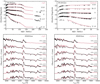 |
Fig. 9. Same as Fig. 8, but now showing a comparison of SN 2012aw with the model x1p5 (no CSM; left) and model x1p5ext3 (with CSM; right). The main effect of the CSM is to produce a slightly more luminous SN which peaks earlier, and which is in better agreement with observations. However the model is slightly too blue for the first month. This could probably be remedied by changes in the structure of the CSM. The spectroscopic comparisons after 30 d are very similar. |
As SN 2012aw is similar to SN 1999em, Morozova et al. (2018) propose a similar model. While our model x1p5ext3 has a similar CSM mass, it has the same discrepancy with the results of Morozova et al. (2018) – our progenitor radius is smaller and the explosion energy is larger. We surmise that the dynamical properties of their model would be in tension with the spectroscopic properties of SN 2012aw. SN 2012aw has also been studied by Dall’Ora et al. (2014), who propose an ejecta of 20 M⊙, a kinetic energy of 1.5 × 1051 erg, and a 56Ni mass of 0.06 M⊙. They do not discuss the adopted density structure of the progenitor. The spectral information used to constrain the ejecta expansion rate is primarily limited to a Sc II line (a Fe II line shows the same velocity characteristics), with the first “constraining” data point at 40 d after the explosion.
Given the agreement obtained in Fig. 9, a 15 M⊙ progenitor model exploding with an H-rich envelope mass of about 9.5 M⊙, and producing ejecta with about 1.2 × 1051 erg kinetic energy and 0.06 M⊙ of 56Ni seems compatible with observations. A small contribution from CSM improves the match to the brightness before 15 d, but also causes a slight color discrepancy.
6.1.3. SN 2004et
SN 2004et is associated with NGC 6946 and is one of ten recent SNe known to have occurred in this galaxy (e.g., Kilpatrick & Foley 2018). The estimate of the progenitor’s mass of  by Eldridge & Xiao (2019) is higher than the earlier estimates of
  (Davies & Beasor 2018) and
  (Smartt 2015) primarily due to an increase in the distance to NGC 6946 (from 5.5 to ∼7.8 Mpc; Anand et al. 2018). A detailed multi-wavelength study of SN 2004et was done by Misra et al. (2007) who argue for a 56Ni mass of 0.06 ± 0.03 M⊙ (for d = 5.5 Mpc), an ejecta mass of 8–16 M⊙, and a progenitor mass of around 20 M⊙.
Figure 10 compares the multi-band light curves and multi-epoch spectra of SN 2004et with the model x1p5ext3 that was discussed in the previous section. Here, a reddening E(B − V) = 0.3 mag is used, and with this choice, SN 2004et becomes very similar to SN 2012aw. This lower reddening is more compatible with the color evolution of SN 2004et. It also yields a reasonable match to the color evolution and to the multi-epoch spectra throughout the optical (some dates are less well fit but it is also clear that some spectra have a problematic relative flux calibration). Other reddening values have been used in the literature – Morozova et al. (2018) use E(B − V) = 0.36 mag while Utrobin & Chugai (2009) adopt E(B − V) = 0.41 mag.
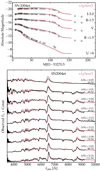 |
Fig. 10. Same as Fig. 8, but now showing a comparison of SN 2004et with the model x1p5ext3 (with CSM). The adopted reddening is E(B − V) = 0.3 mag. |
The model parameters of Morozova et al. (2018) have the same offset as for the SNe discussed above, with a larger progenitor radius and a lower ejecta kinetic energy (the offset also partially arises from their adopted reddening). The good match of model x1p5etx3 to the width of Doppler-broadened profiles in SN 2004et does not seem compatible with the low kinetic energy proposed by Morozova et al. (2018), who ignore spectral constraints.
Our model x1p5ext3 differs from that of Utrobin & Chugai (2009), who use a non-evolutionary progenitor model. Their model parameters correspond to a 1500 R⊙ progenitor radius, an ejecta mass of 24.5 M⊙, an explosion energy of 2.3 × 1051 erg, and a 56Ni mass of 0.068 M⊙. Only the 56Ni mass is close to the 0.053 M⊙ of model x1p5ext3, the offset resulting from the larger reddening used in Utrobin & Chugai (2009). Our model suggests that an evolutionary model works well for SN 2004et, and that there is no need to invoke a very large mass for the progenitor star. A 15 M⊙ progenitor star (similar to our model x1p5ext3) is also proposed by Jerkstrand et al. (2012) based on nebular-phase spectral modeling.
6.2. Comparison to fast decliners
6.2.1. SN 2013ej
SN 2013ej is located in M 74. Fraser et al. (2014) identified a M supergiant as the possible progenitor. Archival studies of the SN field by Johnson et al. (2018) indicate that the progenitor most likely did not have a major outburst in the decade prior to its death. Even at early times SN 2013ej was significantly polarized (∼1%; Leonard et al. 2013; Mauerhan et al. 2017). Mauerhan et al. (2017) argue that the polarization data for SN 2013ej are consistent with an oblate ellipsoidal photosphere viewed nearly edge-on. They also find evidence in nebula spectra that interaction with a CSM is continuing. Evidence for asymmetries is also seen in the Hα profile. Utrobin & Chugai (2017) argue that the Hα asymmetry and the observed level of polarization arise from a strong asymmetry in the distribution of 56Ni.
Figure 11 is analogous to Fig. 9 but now compares a model without CSM (model x3p0) and a model with CSM (model x3p0ext4) with the multi-band light curves and multi-epoch spectra of SN 2013ej. Both models do well after about 30 d, but prior to that, only the model with CSM can capture approximately the bump in radiation (as compared to slow decliners; see Fig. 1).
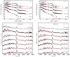 |
Fig. 11. Same as Fig. 8, but now showing a comparison of SN 2013ej with the model x3p0 (no CSM; left) and model x3p0ext4 (with CSM; right). The model with CSM provides a better match to the brightness at early times and the weakness of the emission features, but is too blue, especially at day 14.5. After 50 days the models are very similar. |
Model x3p0 overestimates the line emission strengths early on. It is too faint in all bands (but not by much in U). However, after 50 d, both multi-band light curves (and thus color curves) and optical spectra are well matched. Model x3p0ext4 resolves in part the brightness problem before 30 d, but the color is too blue. Because of the CSM, there is less material at large velocities so the model under-predicts the width of some lines (note, however, that some line profiles have a complex morphology, such as the broad red shoulder in Hα). The early-time spectra are in some ways better matched than with model x3p0, in particular because the model captures the much reduced emission line strengths.
These trends suggest that CSM is indeed a necessary ingredient to reproduce the early-time properties of SN 2013ej but the exact properties of the CSM (mass, extent, or density structure), which may deviate from spherical symmetry, are likely an important component. A more confined CSM distribution would probably help resolve the color offset while preserving a fraction of the boost to the brightness.
6.2.2. SN 2014G
The photometric and spectroscopic evolution of SN 2014G has been extensively discussed by Terreran et al. (2016). Early spectra show high ionization features, such as He II, C IV and a N III/N V blend, indicating interaction of the ejecta with CSM, possibly a pre-existing wind. By comparing the strength of the [O I] λλ6300, 6363 doublet with synthetic spectra, Terreran et al. (2016) deduced a progenitor mass in the range 15–19 M⊙.
Figure 12 compares the photometric and spectroscopic observations of SN 2014G with the results from models x3p0 and x3p0ext5. Because the early-time brightness boost in SN 2014G is greater than in SN 2013ej, the brightness discrepancy with model x3p0 is larger. It is nearly resolved with model x3p0ext5 (CSM mass of 1.97 M⊙) but the model is now too blue up to about 30 d. As before, using a more confined CSM would reduce the color offset. However, the model with CSM yields a better consistency with photometric observations, the featureless spectra at early times, and the weak absorption in Hα at all times.
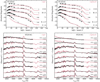 |
Fig. 12. Same as Fig. 8, but now showing a comparison of SN 2014G with the model x3p0 (no CSM; left) and model x3p0ext5 (with CSM; right). The model with the CSM shows much better agreement with the observations – the light curve is better matched at earlier times, the weak Hα P Cygni profiles are in better agreement with observations, and the emission at early times is either weak or absent. |
7. Conclusions
We have presented a set of simulations for Type II SNe arising from two different types of RSG star progenitors. The mdot model set is characterized by progenitors having a range of H-rich envelope mass between 0.9 and 9.5 M⊙, but the same He core mass of about 4 M⊙. The ext set is characterized by a range of CSM mass between 0.02 and 1.97 M⊙ enshrouding the same RSG progenitor star. We compare the SN ejecta and radiation properties for each set of models. We also compare their multi-band light curves and multi-epoch spectra to those of Type II SNe characterized by a range of V-band decline rates (i.e., from slow to fast decliners). All models have the same ejecta kinetic energy.
By reducing the H-rich envelope mass, the bolometric light curve transitions from slow to fast declining and from a long to a short high-brightness phase (i.e., photospheric phase). The V-band light curves are changed in a similar way to the luminosity. The boost at maximum is <1 mag and the rise time is unchanged (here about 20−30 d). Optical colors (or the photospheric temperature) are also unaffected. The smaller the H-rich envelope mass, the larger the maximum ejecta velocity and the broader the P-Cygni profiles at early times.
By increasing the CSM mass located directly above R⋆, the luminosity increases at early times before eventually leveling off at the luminosity for the CSM-less counterpart. The photospheric phase duration is unaffected except for the model with the highest CSM mass. The interaction induced by the CSM reduces the outer ejecta kinetic energy and causes the formation of a dense shell. Hence, unlike for the ext model set, there is an anti-correlation between brightness boost and line width. For a large CSM mass, the early-time spectra are featureless, while at the recombination epoch, the line profiles show weaker absorptions. Hα may show a pure emission profile.
Overall, the luminous fast decliners SNe 2013ej and 2014G are in better agreement with the ext model set, both concerning the multi-band light curves and the spectral evolution in the optical. These two SNe may require 0.5–1 M⊙ of CSM, although the exact value depends on the CSM mass distribution. Interestingly, their H-rich envelope mass is only about 1 M⊙ lower than for the slow decliners, and thus still very massive. It may be that this envelope mass deficit corresponds to the mass excess residing directly above R⋆.
The slow decliners SNe 1999em, 2012aw, and 2004et probably require no more than 0.2 M⊙ confined to the progenitor surface. Here, the CSM acts to reduce the rise time in the V band. We argue, however, that this rise time is nearly matched if one invokes no CSM but a relatively compact RSG star progenitor. Our models with zero up to 0.2 M⊙ of CSM yield compelling evidence that standard RSG star explosions as produced by stellar evolution models can reproduce with fidelity the observed properties of standard SNe II-P.
Because of the inherent complexity of the CSM, it is a challenge to obtain a good match to the early-time observations (light curves as well as spectra) of fast decliners. The influence of the CSM depends on its mass, its density structure, and its maximum extent in radius beyond R⋆. For example, Type IIn spectral signatures can only occur if the photon mean free path in the CSM is large enough to allow for radiation escape through unshocked slow CSM (see, e.g., Dessart et al. 2017).
The effect of the CSM when placed at R⋆ is very different from that at large distances. The main difference is that at R⋆, the CSM is shocked under optically-thick conditions and at a time when the shocked envelope has not yet reached its asymptotic kinetic energy. Interaction with such a CSM first transfers kinetic energy to radiative energy, but because of optical depth effects, this radiative energy is transferred back into kinetic energy. By varying the extent and mass of the CSM, we can modulate the radiative losses at shock breakout and tune the luminosity boost. When interaction occurs at large distances and over large distances, the extracted kinetic energy is converted into radiation energy that escapes. Then, the boost to the luminosity can be very large. Hence, in events such as SN 1979C, or even more so for SN 1998S, the much larger luminosity boost requires the CSM to be detached from R⋆, or extended far above R⋆, so that radiative losses can be much larger. As a result, the interaction model of Dessart et al. (2016) proposed for SN 1998S is much more luminous than the present model x3p0ext4 (which matches roughly the brightness of SN 2013ej, which is much fainter than SN 1998S) even though they have the same CSM mass. Hence, more work is needed to investigate the impact on SN observables of using different types of CSM with a variety of densities, extents, etc. The CSM may also be clumpy and asymmetric, which could affect the predictions made so far assuming 1D.
The models presented here for slow decliners continue to support the notion that Type II SN progenitors may be more compact than typically obtained by stellar evolution models computed with a mixing length parameter of 1.5. There is evidence that inferred RSG radii are smaller if the full spectral energy distribution, rather than the optical range alone, is modeled (Davies et al. 2013). The argument that stellar evolution models predict large RSG radii if the default mixing length parameter is used is not convincing. This default is based on the Sun and may not apply to RSG stars. RSG radii from a few hundred to thousands of R⊙ can be produced by fine-tuning this parameter (Dessart et al. 2013). KEPLER observations suggest that the mixing length differs between red giants and the Sun (Li et al. 2018), although not by as much as adopted here. The situation in RSGs may also differ. That being said, we should reinvestigate to what extent CSM may alter this need for more compact RSG progenitors. It is clear that for events, such as SNe 1979C and 1998S, in which the radiation is strongly influenced by interaction, the progenitor radius has little impact on the observables.
This study is not exhaustive. Our small selection of slow decliners seems to be compatible with a 15 M⊙ progenitor, 0.2 M⊙ or less of CSM, and moderate variations in H-rich envelope mass around 9−10 M⊙. In slow decliners, the inferred CSM, located directly above R⋆, seems to be very confined. It is also probably bound to the star and may be counted as part of the star mass. There is no evidence that it corresponds to a super-wind. The fast decliners (limited here to SNe 2013ej and 2014G) require slightly lower H-rich envelope masses to yield shorter photospheric phase durations. This may arise because they come from higher mass progenitors, which have a greater RSG wind mass-loss rate, or from binaries, although binarity tends to produce pre-SN progenitors with a <1 M⊙ H-rich envelope mass (Yoon et al. 2017).
The definition of the optically-thick phase in Anderson et al. (2014) is distinct from the true optically-thick phase, which lasts until the ejecta optical depth drops to 1, or 2/3. At that time, the bolometric luminosity follows the decay power, and the change of slope from the fall-off from the plateau to the nebular tail is obvious. However, even during the nebular stage optical depth effects must be taken into account when modeling spectra (see, for example, Dessart & Hillier 2011b; Jerkstrand et al. 2012).
Scaling the 56Ni abundance to match a desired value would be inconsistent since all abundances should be scaled. This means that these models should be recomputed with a different piston location or piston trajectory until they produce the same explosive yields. This is beyond the scope of this study.
If we assume that L(t) only represents the total IR, optical and UV luminosity then Q(t) is the radioactive energy absorbed in the envelope.
Acknowledgments
DJH acknowledges partial support from NASA theory grant NNX14AB41G and STScI theory grants HST-AR-12640.01 and HST-AR-14568.001-A. LD thanks ESO-Vitacura for their hospitality.
References
- Anand, G. S., Rizzi, L., & Tully, R. B. 2018, AJ, 156, 105 [NASA ADS] [CrossRef] [Google Scholar]
- Anderson, J. P., González-Gaitán, S., Hamuy, M., et al. 2014, ApJ, 786, 67 [NASA ADS] [CrossRef] [Google Scholar]
- Baron, E., Nugent, P. E., Branch, D., & Hauschildt, P. H. 2004, ApJ, 616, L91 [NASA ADS] [CrossRef] [Google Scholar]
- Bartunov, O. S., & Blinnikov, S. I. 1992, Sov. Astron. Lett., 18, 43 [NASA ADS] [Google Scholar]
- Bersten, M. C., Benvenuto, O., & Hamuy, M. 2011, ApJ, 729, 61 [NASA ADS] [CrossRef] [Google Scholar]
- Blinnikov, S. I., & Bartunov, O. S. 1993, A&A, 273, 106 [NASA ADS] [Google Scholar]
- Bose, S., Kumar, B., Sutaria, F., et al. 2013, MNRAS, 433, 1871 [NASA ADS] [CrossRef] [Google Scholar]
- Chen, X., Kou, S., & Liu, X. 2018, ApJ, submitted [arXiv:1811.03022] [Google Scholar]
- Chugai, N. N. 2006, Astron. Lett., 32, 739 [NASA ADS] [CrossRef] [Google Scholar]
- Chugai, N. N., Chevalier, R. A., & Utrobin, V. P. 2007, ApJ, 662, 1136 [NASA ADS] [CrossRef] [EDP Sciences] [Google Scholar]
- Dall’Ora, M., Botticella, M. T., Pumo, M. L., et al. 2014, ApJ, 787, 139 [NASA ADS] [CrossRef] [Google Scholar]
- Davies, B., & Beasor, E. R. 2018, MNRAS, 474, 2116 [Google Scholar]
- Davies, B., Kudritzki, R.-P., Plez, B., et al. 2013, ApJ, 767, 3 [NASA ADS] [CrossRef] [Google Scholar]
- Dessart, L., & Hillier, D. J. 2005, A&A, 439, 671 [NASA ADS] [CrossRef] [EDP Sciences] [Google Scholar]
- Dessart, L., & Hillier, D. J. 2006, A&A, 447, 691 [NASA ADS] [CrossRef] [EDP Sciences] [Google Scholar]
- Dessart, L., & Hillier, D. J. 2011a, MNRAS, 415, 3497 [NASA ADS] [CrossRef] [Google Scholar]
- Dessart, L., & Hillier, D. J. 2011b, MNRAS, 410, 1739 [NASA ADS] [Google Scholar]
- Dessart, L., & Hillier, D. J. 2019a, A&A, 625, A9 [NASA ADS] [CrossRef] [EDP Sciences] [Google Scholar]
- Dessart, L., & Hillier, D. J. 2019b, A&A, 622, A70 [NASA ADS] [CrossRef] [EDP Sciences] [Google Scholar]
- Dessart, L., Blondin, S., Brown, P. J., et al. 2008, ApJ, 675, 644 [NASA ADS] [CrossRef] [Google Scholar]
- Dessart, L., Livne, E., & Waldman, R. 2010a, MNRAS, 408, 827 [NASA ADS] [CrossRef] [Google Scholar]
- Dessart, L., Livne, E., & Waldman, R. 2010b, MNRAS, 405, 2113 [NASA ADS] [Google Scholar]
- Dessart, L., Hillier, D. J., Waldman, R., & Livne, E. 2013, MNRAS, 433, 1745 [NASA ADS] [CrossRef] [Google Scholar]
- Dessart, L., Gutierrez, C. P., Hamuy, M., et al. 2014, MNRAS, 440, 1856 [NASA ADS] [CrossRef] [Google Scholar]
- Dessart, L., Hillier, D. J., Audit, E., Livne, E., & Waldman, R. 2016, MNRAS, 458, 2094 [NASA ADS] [CrossRef] [Google Scholar]
- Dessart, L., John Hillier, D., & Audit, E. 2017, A&A, 605, A83 [NASA ADS] [CrossRef] [EDP Sciences] [Google Scholar]
- Eldridge, J. J., & Xiao, L. 2019, MNRAS, 485, L58 [NASA ADS] [CrossRef] [Google Scholar]
- Eldridge, J. J., Xiao, L., Stanway, E. R., Rodrigues, N., & Guo, N. Y. 2018, PASA, 35, 49 [NASA ADS] [CrossRef] [Google Scholar]
- Elmhamdi, A., Danziger, I. J., Chugai, N., et al. 2003, MNRAS, 338, 939 [NASA ADS] [CrossRef] [Google Scholar]
- Fassia, A., Meikle, W. P. S., Vacca, W. D., et al. 2000, MNRAS, 318, 1093 [NASA ADS] [CrossRef] [Google Scholar]
- Fassia, A., Meikle, W. P. S., Chugai, N., et al. 2001, MNRAS, 325, 907 [NASA ADS] [CrossRef] [Google Scholar]
- Förster, F., Moriya, T. J., Maureira, J. C., et al. 2018, Nat. Astron., 2, 808 [NASA ADS] [CrossRef] [Google Scholar]
- Fraser, M. 2016, MNRAS, 456, L16 [NASA ADS] [CrossRef] [Google Scholar]
- Fraser, M., Maund, J. R., Smartt, S. J., et al. 2012, ApJ, 759, L13 [NASA ADS] [CrossRef] [Google Scholar]
- Fraser, M., Maund, J. R., Smartt, S. J., et al. 2014, MNRAS, 439, L56 [NASA ADS] [CrossRef] [Google Scholar]
- Gall, E. E. E., Polshaw, J., Kotak, R., et al. 2015, A&A, 582, A3 [NASA ADS] [CrossRef] [EDP Sciences] [Google Scholar]
- González-Gaitán, S., Tominaga, N., Molina, J., et al. 2015, MNRAS, 451, 2212 [NASA ADS] [CrossRef] [Google Scholar]
- Gräfener, G., & Vink, J. S. 2016, MNRAS, 455, 112 [NASA ADS] [CrossRef] [Google Scholar]
- Groh, J. H. 2014, A&A, 572, L11 [NASA ADS] [CrossRef] [EDP Sciences] [Google Scholar]
- Guillochon, J., Parrent, J., Kelley, L. Z., & Margutti, R. 2017, ApJ, 835, 64 [NASA ADS] [CrossRef] [Google Scholar]
- Gutiérrez, C. P., Anderson, J. P., Hamuy, M., et al. 2014, ApJ, 786, L15 [NASA ADS] [CrossRef] [Google Scholar]
- Gutiérrez, C. P., Anderson, J. P., Hamuy, M., et al. 2017a, ApJ, 850, 90 [NASA ADS] [CrossRef] [Google Scholar]
- Gutiérrez, C. P., Anderson, J. P., Hamuy, M., et al. 2017b, ApJ, 850, 89 [NASA ADS] [CrossRef] [Google Scholar]
- Gutiérrez, C. P., Anderson, J. P., Sullivan, M., et al. 2018, MNRAS, 479, 3232 [NASA ADS] [CrossRef] [Google Scholar]
- Guy, J., Sullivan, M., Conley, A., et al. 2010, A&A, 523, A7 [NASA ADS] [CrossRef] [EDP Sciences] [Google Scholar]
- Hamuy, M. 2003, ApJ, 582, 905 [NASA ADS] [CrossRef] [Google Scholar]
- Hamuy, M., Pinto, P. A., Maza, J., et al. 2001, ApJ, 558, 615 [NASA ADS] [CrossRef] [Google Scholar]
- Heger, A., Jeannin, L., Langer, N., & Baraffe, I. 1997, A&A, 327, 224 [NASA ADS] [Google Scholar]
- Hillier, D. J., & Dessart, L. 2012, MNRAS, 424, 252 [NASA ADS] [CrossRef] [Google Scholar]
- Hoflich, P. 1991, A&A, 246, 481 [NASA ADS] [Google Scholar]
- Jeffery, D. J. 1991, ApJ, 375, 264 [NASA ADS] [CrossRef] [Google Scholar]
- Jerkstrand, A., Fransson, C., Maguire, K., et al. 2012, A&A, 546, A28 [NASA ADS] [CrossRef] [EDP Sciences] [Google Scholar]
- Jerkstrand, A., Smartt, S. J., Fraser, M., et al. 2014, MNRAS, 439, 3694 [NASA ADS] [CrossRef] [Google Scholar]
- Johnson, S. A., Kochanek, C. S., & Adams, S. M. 2018, MNRAS, 480, 1696 [NASA ADS] [Google Scholar]
- Katz, B., Kushnir, D., & Dong, S. 2013, ArXiv e-prints [arXiv:1301.6766] [Google Scholar]
- Kilpatrick, C. D., & Foley, R. J. 2018, MNRAS, 481, 2536 [NASA ADS] [CrossRef] [Google Scholar]
- Le Bertre, T., Matthews, L. D., Gérard, E., & Libert, Y. 2012, MNRAS, 422, 3433 [NASA ADS] [CrossRef] [Google Scholar]
- Leonard, D. C., Filippenko, A. V., Barth, A. J., & Matheson, T. 2000, ApJ, 536, 239 [NASA ADS] [CrossRef] [Google Scholar]
- Leonard, D. C., Filippenko, A. V., Gates, E. L., et al. 2002, PASP, 114, 35 [NASA ADS] [CrossRef] [Google Scholar]
- Leonard, D. C., Filippenko, A. V., Ganeshalingam, M., et al. 2006, Nature, 440, 505 [NASA ADS] [CrossRef] [PubMed] [Google Scholar]
- Leonard, D. C., Pignata, G., Dessart, L., et al. 2012, ATel, 4033 [Google Scholar]
- Leonard, D. C., Pignata, G., Dessart, L., et al. 2013, ATel, 5275, 1 [NASA ADS] [Google Scholar]
- Li, C., Hillier, D. J., & Dessart, L. 2012, MNRAS, 426, 1671 [NASA ADS] [CrossRef] [Google Scholar]
- Li, T., Bedding, T. R., Huber, D., et al. 2018, MNRAS, 475, 981 [NASA ADS] [CrossRef] [Google Scholar]
- Lisakov, S. M., Dessart, L., Hillier, D. J., Waldman, R., & Livne, E. 2017, MNRAS, 466, 34 [NASA ADS] [CrossRef] [Google Scholar]
- Lisakov, S. M., Dessart, L., Hillier, D. J., Waldman, R., & Livne, E. 2018, MNRAS, 473, 3863 [NASA ADS] [CrossRef] [Google Scholar]
- Litvinova, I. Y., & Nadezhin, D. K. 1985, Sov. Astron. Lett., 11, 145 [NASA ADS] [Google Scholar]
- Livne, E. 1993, ApJ, 412, 634 [NASA ADS] [CrossRef] [Google Scholar]
- Mackey, J., Mohamed, S., Gvaramadze, V. V., et al. 2014, Nature, 512, 282 [NASA ADS] [CrossRef] [Google Scholar]
- Mauerhan, J. C., Van Dyk, S. D., Johansson, J., et al. 2017, ApJ, 834, 118 [NASA ADS] [CrossRef] [Google Scholar]
- Meynet, G., Chomienne, V., Ekström, S., et al. 2015, A&A, 575, A60 [NASA ADS] [CrossRef] [EDP Sciences] [Google Scholar]
- Misra, K., Pooley, D., Chandra, P., et al. 2007, MNRAS, 381, 280 [NASA ADS] [CrossRef] [Google Scholar]
- Moriya, T. J., Pruzhinskaya, M. V., Ergon, M., & Blinnikov, S. I. 2016, MNRAS, 455, 423 [NASA ADS] [CrossRef] [Google Scholar]
- Moriya, T. J., Yoon, S.-C., Gräfener, G., & Blinnikov, S. I. 2017, MNRAS, 469, L108 [NASA ADS] [CrossRef] [Google Scholar]
- Morozova, V., Piro, A. L., Renzo, M., et al. 2015, ApJ, 814, 63 [NASA ADS] [CrossRef] [Google Scholar]
- Morozova, V., Piro, A. L., & Valenti, S. 2017, ApJ, 838, 28 [NASA ADS] [CrossRef] [Google Scholar]
- Morozova, V., Piro, A. L., & Valenti, S. 2018, ApJ, 858, 15 [NASA ADS] [CrossRef] [Google Scholar]
- Nakar, E., Poznanski, D., & Katz, B. 2016, ApJ, 823, 127 [NASA ADS] [CrossRef] [Google Scholar]
- O’Gorman, E., Kervella, P., Harper, G. M., et al. 2017, A&A, 602, L10 [NASA ADS] [CrossRef] [EDP Sciences] [Google Scholar]
- Ohnaka, K. 2017, in The Lives and Death-Throes of Massive Stars, eds. J. J. Eldridge, J. C. Bray, L. A. S. McClelland, & L. Xiao, IAU Symp., 329, 97 [NASA ADS] [Google Scholar]
- Panagia, N., Vettolani, G., Boksenberg, A., et al. 1980, MNRAS, 192, 861 [NASA ADS] [Google Scholar]
- Pastorello, A., Zampieri, L., Turatto, M., et al. 2004, MNRAS, 347, 74 [NASA ADS] [CrossRef] [Google Scholar]
- Pastorello, A., Valenti, S., Zampieri, L., et al. 2009, MNRAS, 394, 2266 [NASA ADS] [CrossRef] [Google Scholar]
- Patat, F., Barbon, R., Cappellaro, E., & Turatto, M. 1994, A&A, 282, 731 [NASA ADS] [Google Scholar]
- Paxton, B., Bildsten, L., Dotter, A., et al. 2011, ApJS, 192, 3 [Google Scholar]
- Paxton, B., Cantiello, M., Arras, P., et al. 2013, ApJS, 208, 4 [NASA ADS] [CrossRef] [Google Scholar]
- Paxton, B., Schwab, J., Bauer, E. B., et al. 2018, ApJS, 234, 34 [NASA ADS] [CrossRef] [EDP Sciences] [Google Scholar]
- Pooley, D., Lewin, W. H. G., Fox, D. W., et al. 2002, ApJ, 572, 932 [NASA ADS] [CrossRef] [Google Scholar]
- Popov, D. V. 1993, ApJ, 414, 712 [Google Scholar]
- Sahu, D. K., Anupama, G. C., Srividya, S., & Muneer, S. 2006, MNRAS, 372, 1315 [NASA ADS] [CrossRef] [Google Scholar]
- Sako, M., Bassett, B., Becker, A. C., et al. 2014, VizieR Online Data Catalog: II/333 [Google Scholar]
- Sanders, N. E., Soderberg, A. M., Gezari, S., et al. 2015, ApJ, 799, 208 [NASA ADS] [CrossRef] [Google Scholar]
- Shapiro, P. R., & Sutherland, P. G. 1982, ApJ, 263, 902 [NASA ADS] [CrossRef] [Google Scholar]
- Smartt, S. J. 2015, PASA, 32, e016 [NASA ADS] [CrossRef] [Google Scholar]
- Smith, N., Mauerhan, J. C., Cenko, S. B., et al. 2015, MNRAS, 449, 1876 [NASA ADS] [CrossRef] [Google Scholar]
- Spiro, S., Pastorello, A., Pumo, M. L., et al. 2014, MNRAS, 439, 2873 [NASA ADS] [CrossRef] [Google Scholar]
- Sukhbold, T., Ertl, T., Woosley, S. E., Brown, J. M., & Janka, H.-T. 2016, ApJ, 821, 38 [Google Scholar]
- Terreran, G., Jerkstrand, A., Benetti, S., et al. 2016, MNRAS, 462, 137 [NASA ADS] [CrossRef] [Google Scholar]
- Ugliano, M., Janka, H.-T., Marek, A., & Arcones, A. 2012, ApJ, 757, 69 [NASA ADS] [CrossRef] [Google Scholar]
- Utrobin, V. P. 2007, A&A, 461, 233 [NASA ADS] [CrossRef] [EDP Sciences] [Google Scholar]
- Utrobin, V. P., & Chugai, N. N. 2009, A&A, 506, 829 [NASA ADS] [CrossRef] [EDP Sciences] [Google Scholar]
- Utrobin, V. P., & Chugai, N. N. 2017, MNRAS, 472, 5004 [NASA ADS] [CrossRef] [Google Scholar]
- Utrobin, V. P., Wongwathanarat, A., Janka, H.-T., & Müller, E. 2017, ApJ, 846, 37 [NASA ADS] [CrossRef] [Google Scholar]
- Van Dyk, S. D., Cenko, S. B., Poznanski, D., et al. 2012, ApJ, 756, 131 [NASA ADS] [CrossRef] [Google Scholar]
- Woosley, S. E., & Heger, A. 2007, Phys. Rep., 442, 269 [NASA ADS] [CrossRef] [Google Scholar]
- Yaron, O., & Gal-Yam, A. 2012, PASP, 124, 668 [NASA ADS] [CrossRef] [Google Scholar]
- Yaron, O., Perley, D. A., Gal-Yam, A., et al. 2017, Nat. Phys., 13, 510 [NASA ADS] [CrossRef] [Google Scholar]
- Yoon, S.-C., Woosley, S. E., & Langer, N. 2010, ApJ, 725, 940 [NASA ADS] [CrossRef] [Google Scholar]
- Yoon, S.-C., Dessart, L., & Clocchiatti, A. 2017, ApJ, 840, 10 [NASA ADS] [CrossRef] [Google Scholar]
- Yuan, F., Jerkstrand, A., Valenti, S., et al. 2016, MNRAS, 461, 2003 [NASA ADS] [CrossRef] [Google Scholar]
- Zhang, W., Woosley, S. E., & Heger, A. 2008, ApJ, 679, 639 [NASA ADS] [CrossRef] [Google Scholar]
Appendix A: Energy conservation
For a homologous flow we have the global comoving-frame energy constraint
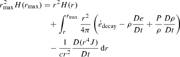 (A.1)
(A.1)
(Hillier & Dessart 2012). Multiplying by 16π2t and integrating from some initial time t0 to t yields
![Mathematical equation: $$ \begin{aligned} \int ^t_{t_0} t L(t) \,\mathrm{d}t = \int ^t_{t_0} [t Q(t) - t I(t)] \,\mathrm{d}t + t_0E(t_0) - t E(t). \end{aligned} $$](/articles/aa/full_html/2019/11/aa35100-19/aa35100-19-eq8.gif) (A.2)
(A.2)
In the above
 (A.3)
(A.3)
 (A.4)
(A.4)
and is the total energy emitted by radioactive decays3, and E(t) is the total radiative energy of the envelope at time t. It arises because
![Mathematical equation: $$ \begin{aligned} \int ^t_{t_0} 16 \pi ^2 t&\int _{r_{\rm min}}^{r_{\rm max}} {1 \over cr^2} {D(r^4 J) \over Dt}\,\, \mathrm{d}r \, \mathrm{d}t \\ =&\int ^t_{t_0} 16 \pi ^2 t \int _{V_{\rm min}}^{V_{\rm max}} {1 \over c V^2 t^2} {D(r^4 J) \over Dt}\,\, t \,\mathrm{d}V \, \mathrm{d}t \\ =&\int _{r_{\rm min}}^{r_{\rm max}} 4\pi r^2 \left[ t 4\pi J/c \right]^t_{t_0} \,\mathrm{d}r\\ =&tE(t)-t_0E(t_0) \end{aligned} $$](/articles/aa/full_html/2019/11/aa35100-19/aa35100-19-eq11.gif)
In Eq. (A.2) the luminosity at the inner boundary is taken as zero. The factor of t in the equation allows for the influence of adiabatic expansion. This equation would need to be modified in the presence of alternate energy sources such as a magnetar.
An approximate form of Eq. (A.2) is
 (A.5)
(A.5)
since the gas-pressure terms are generally subservient to the radiation and decay terms, and can be neglected. Versions of the above equation (but in the observer’s frame) have been provided by Katz et al. (2013) who pointed out that the 56Ni mass in Type Ia SNe can be derived by integrating the observed luminosity. Nakar et al. (2016) later used a more general equation in a study of Type II-P SNe.
Valid for non-interacting SNe, Eq. (A.5) highlights the two distinct mechanisms that produce the observed light curve. In a generic Type Ia SN, the radiative energy in the ejecta is “initially” small due to the rapid expansion from an Earth-size object (r < 109 cm) to 1014 cm on a time scale of one day. As a consequence the SN is initially faint. The luminosity of the SN increases as the energy deposited by radioactive decay in the interior diffuses to the surface, and the entire light curve is powered by nuclear decay – primarily 56Ni and its daughter isotope, 56Co.
Type II-P SNe represent the other extreme. The progenitor is a RSG with an initial radius of ∼500 R⊙. With the large radius and Teff ∼ 2 × 10⁵ K at breakout, we see a rapid brightening of the SN. To a large extent the light curve is determined by the initial temperature structure of the ejecta. A recombination wave moves into the ejecta allowing stored and trapped thermal energy to be released. This release controls the early part of the light curve. At later times energy released by radioactive decay becomes increasingly important, and it is the dominant power source in the nebular phase. In Fig. A.1 we illustrate the various terms for model x3p0.
 |
Fig. A.1. Comparison of various terms in Eq. (A.2) for model x3p0. The red curve shows |


The practical importance of Eq. (A.2) is that it can be used to check the accuracy of the calculations. While Eq. (A.1) provides a check on the accuracy of the calculation at a single time step, it does not provide any indication of the accuracy over multiple time steps. However we can use Eq. (A.2), and such a check is now available with our CMFGEN calculations. Using this check we did discover a small, but systematic, energy loss in models but which had very little influence on resultant spectra. In the zeroth-moment equation we have a term containing Dr4J/Dt which is equivalent to rDr3J/Dt + r3VJ. For historical reasons we used the latter form for differencing, however differencing the first form provides greater accuracy.
Appendix B: Light curve comparison between CMFGEN and V1D
Figure B.1 compares the bolometric light curves obtained with V1D and CMFGEN for the ext model set. CMFGEN simulations are started when the ejecta is close to homologous expansion, typically between 10 and 20 d after explosion (it takes longer for models such as x3p0ext6 with a massive and extended CSM). These two 1D codes differ in many ways. The code V1D solves the radiation hydrodynamics equations using gray flux-limited diffusion and assuming the gas is in LTE at each depth. CMFGEN ignores dynamical effects but solves the radiative transfer equation and the statistical equilibrium equations, accounting for the effects of line and continuum processes, as well as non-thermal and time-dependent effects. Despite these many differences, the bolometric light curves obtained with the two codes are in rough agreement. An offset is visible at the end of the photospheric phase, but it is small. In CMFGEN, the luminosity is higher at the end of the photospheric phase. This depletes the stored energy faster and causes an earlier transition to the nebular phase.
 |
Fig. B.1. Bolometric light curve comparison between CMFGEN (solid) and V1D (dashed) for model x3p0 and variants with a dense atmosphere. We show the results for V1D only past 1 d after shock breakout. |
Appendix C: Temperature evolution
In Fig. C.1 we illustrate the temperature evolution for model x3p0 (solid), and model x3p0ext4 (dashed). As to be expected, the outer region of the x3p0ext4 model is hotter because of the interaction of the ejecta and radiation field with the CSM. At depth the temperature evolution is unchanged by the CSM.
 |
Fig. C.1. Comparison of the temporal evolution of the temperature for model x3p0 and model x3p0ext4. The influence of the CSM on the temperature structure is easily seen. |
All Tables
All Figures
|
Fig. 1. Sample of observed V-band light curves, corrected for extinction and reddening, illustrating the well known diversity of Type II SNe (e.g., Patat et al. 1994; Pastorello et al. 2004). This diversity is representative of that shown in Anderson et al. (2014), revealing Type II SNe with a range of brightness, decline rate, and duration in their high-brightness phase. The plotting order progresses from faint to bright events at maximum (see Sect. 2.2 for discussion). |
| In the text | |
|
Fig. 2. Comparison of spectra in the Hα region at about 15 and 60 d after the inferred time of explosion for a set of observed Type II SNe with a range of V-band decline rates during the photospheric phase. The spectra have been normalized so that the peak value (in the spectral window shown) is unity, with an additional offset of unity for the upper spectrum. Left-most two columns: standard Type II SNe with a slow decline rate. Third column: SNe that exhibit a much larger brightness at early times followed by a fast decline. Rightmost column: SNe with a huge early-time brightness and a fast decline rate at all times. The photometric differences between these families of events have a clear spectroscopic counterpart (see Sect. 2.3 for discussion). |
| In the text | |
|
Fig. 3. Left: mass density versus Lagrangian mass (top) and radius (bottom) at the onset of core collapse for the set of 15 M⊙ simulations produced with MESA using a mixing-length parameter of 3 and a variety of mass-loss rate scalings during the RSG phase. Right: same as left, but now for variants of model x3p0 in which some CSM has been added. The corresponding model properties are given in Table 2. |
| In the text | |
|
Fig. 4. Left: evolution of the bolometric luminosity (top), the photospheric velocity (middle), and the photospheric temperature (bottom) for the explosion models computed by V1D and based on the mdot model set. Right: same as left, but now for the ext model set (see Sect. 4 for discussion). |
| In the text | |
|
Fig. 5. Left: illustration of the absolute V-band light curves (top), the spectral region centered on Hα at about 20 d after explosion (middle), and the U − V and V − I color curves (bottom) for the mdot simulations performed with CMFGEN. Right: same as left, but now for the ext model set (see Sect. 5 for discussion). |
| In the text | |
|
Fig. 6. Comparison of spectra in the Hα region at about 15 and 50 d after explosion for the model set with decreasing H-rich envelope mass (from x1p5 to x1e1). |
| In the text | |
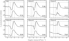 |
Fig. 7. Same as Fig. 6, but now for the model set with increasing CSM mass (from x3p0 to x3p0ext6). |
| In the text | |
|
Fig. 8. Comparison of multi-band light curves (left) and multi-epoch spectra (right) for SN 1999em and model x2p0. The time origin is the inferred time of explosion. For the spectral comparison, the model is redshifted and reddened, and the label ΔMV gives the V-band magnitude offset at each epoch. The spectra are normalized to each other and shifted for better visibility. |
| In the text | |
|
Fig. 9. Same as Fig. 8, but now showing a comparison of SN 2012aw with the model x1p5 (no CSM; left) and model x1p5ext3 (with CSM; right). The main effect of the CSM is to produce a slightly more luminous SN which peaks earlier, and which is in better agreement with observations. However the model is slightly too blue for the first month. This could probably be remedied by changes in the structure of the CSM. The spectroscopic comparisons after 30 d are very similar. |
| In the text | |
|
Fig. 10. Same as Fig. 8, but now showing a comparison of SN 2004et with the model x1p5ext3 (with CSM). The adopted reddening is E(B − V) = 0.3 mag. |
| In the text | |
|
Fig. 11. Same as Fig. 8, but now showing a comparison of SN 2013ej with the model x3p0 (no CSM; left) and model x3p0ext4 (with CSM; right). The model with CSM provides a better match to the brightness at early times and the weakness of the emission features, but is too blue, especially at day 14.5. After 50 days the models are very similar. |
| In the text | |
|
Fig. 12. Same as Fig. 8, but now showing a comparison of SN 2014G with the model x3p0 (no CSM; left) and model x3p0ext5 (with CSM; right). The model with the CSM shows much better agreement with the observations – the light curve is better matched at earlier times, the weak Hα P Cygni profiles are in better agreement with observations, and the emission at early times is either weak or absent. |
| In the text | |
|
Fig. A.1. Comparison of various terms in Eq. (A.2) for model x3p0. The red curve shows |
| In the text | |
|
Fig. B.1. Bolometric light curve comparison between CMFGEN (solid) and V1D (dashed) for model x3p0 and variants with a dense atmosphere. We show the results for V1D only past 1 d after shock breakout. |
| In the text | |
|
Fig. C.1. Comparison of the temporal evolution of the temperature for model x3p0 and model x3p0ext4. The influence of the CSM on the temperature structure is easily seen. |
| In the text | |
Current usage metrics show cumulative count of Article Views (full-text article views including HTML views, PDF and ePub downloads, according to the available data) and Abstracts Views on Vision4Press platform.
Data correspond to usage on the plateform after 2015. The current usage metrics is available 48-96 hours after online publication and is updated daily on week days.
Initial download of the metrics may take a while.