| Issue |
A&A
Volume 698, June 2025
|
|
|---|---|---|
| Article Number | A213 | |
| Number of page(s) | 12 | |
| Section | Stellar structure and evolution | |
| DOI | https://doi.org/10.1051/0004-6361/202554128 | |
| Published online | 17 June 2025 | |
SN 2023ixf: Interaction signatures in the spectrum at 445 days
1
Instituto de Astrofísica de La Plata (IALP), CONICET – UNLP, La Plata, Argentina
2
Facultad de Ciencias Astronómicas y Geofísicas, Universidad Nacional de La Plata (UNLP), Av. Centenario s/n B1900FWA, La Plata, Argentina
3
Kavli Institute for the Physics and Mathematics of the Universe (WPI), The University of Tokyo Institutes for Advanced Study, The University of Tokyo, Kashiwa, 277-8583 Chiba, Japan
4
Tuorla Observatory, Department of Physics and Astronomy, 20014 University of Turku, Turku, Finland
5
Finnish Centre for Astronomy with ESO (FINCA), 20014 University of Turku, Turku, Finland
6
Department of Astronomy, Kyoto University, Kitashirakawa-Oiwake-cho, Sakyo-ku, Kyoto 606-8502, Japan
⋆ Corresponding author: This email address is being protected from spambots. You need JavaScript enabled to view it.
Received:
13
February
2025
Accepted:
11
May
2025
Abstract
Context. SN 2023ixf is one of the nearest and brightest Type II supernovae (SNe) of the past decades. Its proximity and extremely early discovery have enabled a large number of studies based on extensive observations throughout the electromagnetic spectrum. A rich set of pre-explosion data provided important insight into the properties of the progenitor star. There has been, however, a wide range of estimated initial masses of 9–22 M⊙. Early monitoring of the SN also showed the presence of a dense circumstellar material (CSM) structure near the star (≲1015 cm), which was probably expelled in the last years prior to the explosion. At farther distances, there have been indications of a drop in the CSM density. These extended CSM structures can be further probed with late-time observations during the nebular phase.
Aims. We monitored the spectroscopic evolution of SN 2023ixf at late phases with the aim of characterizing the progenitor properties. The observations also serve to search for indications of ejecta–CSM interaction that may shed light on the mass-loss processes during the final stages of evolution of the progenitor star.
Methods. This study is based on a nebular spectrum obtained with GMOS at the Gemini North Telescope 445 days after explosion. The SN evolution was analyzed in comparison with a previous spectrum at an age of 259 days. The 445 d spectrum was further compared with those of similar SNe II and with synthetic radiation-transfer nebular spectra. Line profiles were used to determine properties of the emitting regions. [O I] and [Ca II] line fluxes were used to derive an estimate of the progenitor mass at birth.
Results. The 445 d spectrum exhibits a dramatic evolution with signs of ejecta–CSM interaction. The Hα profile shows a complex profile that can be separated into a boxy component, possibly arising from the interaction with a CSM shell and a centrally peaked component that may be due to the radioactive-powered SN ejecta. The CSM shell would be located at a distance of ∼1016 cm from the progenitor, and it may be associated with mass loss occurring up until ≈500−1000 years before the explosion. Similar interaction signatures have been detected in other SNe II, although for events with standard plateau durations, this occurred later than 600–700 days. SN 2023ixf appears to belong to a group of SNe II with short plateaus or linear light curves that develop interaction features before ≈500 days. Other lines, such as those from [O I] and [Ca II], appear to be unaffected by the CSM interaction. This allowed us to estimate an initial progenitor mass, which falls in the relatively low range of 10–15 M⊙.
Key words: supernovae: general / supernovae: individual: SN 2023ixf
© The Authors 2025
 Open Access article, published by EDP Sciences, under the terms of the Creative Commons Attribution License (https://creativecommons.org/licenses/by/4.0), which permits unrestricted use, distribution, and reproduction in any medium, provided the original work is properly cited.
This article is published in open access under the Subscribe to Open model. This email address is being protected from spambots. You need JavaScript enabled to view it. to support open access publication.
1. Introduction
Mass loss plays a critical role in the evolution and final fate of massive stars. The structure of the star at core collapse as well as the distribution of circumstellar material (CSM) due to mass-loss processes dictates the observational properties of the ensuing supernova (SN) event. This means that studying supernovae (SNe) can provide important insight into this issue.
The most common type of core-collapse SN is that with hydrogen-dominated spectra, known as Type II SNe (SNe II). These events have been associated with red supergiant (RSG) stars that retain most of their H-rich envelopes (Smartt et al. 2009; Van Dyk et al. 2012; Smartt 2015). Historically, it appeared that SN II progenitors suffered only mild mass loss during their evolution. However, in the past decade, there has been mounting evidence of substantial mass loss at least in the final stages of evolution (e.g., see Förster et al. 2018).
There is a variety of interaction signatures that can be identified through early observations of SNe II. These include high luminosity, especially in the ultraviolet, and blue colors (Dessart & Hillier 2022; Jacobson-Galán et al. 2024; Moriya et al. 2023); a delayed rise to maximum light (Moriya et al. 2018; Förster et al. 2018); radio and X-ray emission from nonthermal processes in the interaction region (Chevalier & Fransson 2017; Matsuoka et al. 2019; Moriya 2021); high-velocity absorption features in the spectra (Chugai et al. 2007; Gutiérrez et al. 2017; Dessart & Hillier 2022); and short-duration, narrow emission lines in the optical spectra during the first days or week after the explosion (also known as “flash features”; Yaron et al. 2017; Bruch et al. 2023; Jacobson-Galán et al. 2024).
These observations probe CSM structures that typically extend to 1014−1015 cm and must be formed during the final months to years prior to the explosion, given the typical RSG wind velocities. The associated mass-loss rates are  M⊙ yr−1, which is orders of magnitude larger than what is measured in RSG stars (Beasor et al. 2020) and than that predicted by standard wind-powering mechanisms in isolated stars (Vink et al. 2001). This discrepancy has led to the suggestion of alternative mass-loss mechanisms via accelerated winds (Moriya et al. 2017), episodic outbursts, or mass transfer in interacting binaries (see a review in Smith 2014).
Late-time indications of ejecta–CSM interaction have also been reported for SNe II in the form of complex, flat-topped, or boxy1 Hα emission profiles, usually accompanied by a flattening of the light curves due to the extra power released by the interaction. There is a wide range of ages when this interaction signature is detected. For several SNe II with particularly short plateaus or those with linear or fast-declining light curves, this behavior was observed to start as soon as ∼200−500 days after the explosion (several examples are listed in Section 3.1 and in the Introduction sections of Weil et al. 2020; Dessart et al. 2023). This is in contrast with the lack of boxy or flat-topped Hα profiles reported at ages between ≈150 and 500 days among 38 normal-plateau SNe II in the sample of Silverman et al. (2017)2. Only a handful of SNe II with standard plateau durations have shown similar signatures but at ages later than ≈600 days. Given the dimness of SNe at ages of several hundred days and later and the ensuing lack of coverage, it is currently not possible to establish the actual fraction of SNe II that undergo this transformation from radioactive-powered to interaction-powered evolution. However, because mass loss is ubiquitous among massive stars, this transition should eventually occur in all core-collapse SNe (Dessart & Hillier 2022). Based on this, the question should concern the timescale of the transition rather than about the fraction of objects that suffer it.
The late-time interaction features probe CSM structures located at greater distances of ∼1015−1016 cm from the progenitor star. This material must have been expelled by the star in the final centuries before the explosion. The appearance of box-like Hα profiles in the standard-plateau SNe II SN 2004et and SN 2017eaw has been associated with mass loss rates of  M⊙ yr−1, in agreement with estimates from radio and X-ray observations (Kotak et al. 2009; Weil et al. 2020). This is well in line with the estimated mass loss rates for RSG stars.
By introducing a constant power source due to interaction in radiative transfer calculations of SNe II, Dessart & Hillier (2022) were able to qualitatively reproduce the photometric and spectroscopic features attributed to interaction, such as enhanced UV emission, high-velocity absorptions during the plateau phase, and the development of boxy Hα profiles during the nebular phase. Dessart et al. (2023) extend the analysis to later times and find a good agreement with the overall evolution of several SNe II that showed signs of interaction in the form of boxy Hα emission and light-curve flattening.
In the present work, we analyze a nebular spectrum of the nearby Type II SN 2023ixf obtained at 445 days after the explosion. The new spectrum shows a dramatic evolution in comparison with the 259 d nebular spectrum published by Ferrari et al. (2024) (F24, hereafter), especially in the appearance of a boxy Hα profile. While the present analysis was under development, an additional spectrum of SN 2023ixf at 363 days was made public by Kumar et al. (2025) where the boxy Hα profile had already emerged. More recently, Michel et al. (2025), Zheng et al. (2025), and Li et al. (2025) presented thorough spectroscopic follow-up observations reaching until 413, 442, and 407 days, respectively, where this evolution of the Hα profile is observed. This clearly indicates that SN 2023ixf belongs to the group of SNe II that showed interaction signatures during the nebular phase prior to ∼500 days. This is in line with the relatively short plateau phase of ≈80 days that was observed for this SN (Bersten et al. 2024).
Given its proximity, SN 2023ixf has provided a wealth of observational data that shed light on the nature of its progenitor star and properties of its CSM. Early-time observations indicated the presence of a dense CSM confined within ≲1015 cm that was associated with enhanced mass loss with rates of  M⊙ yr−1 during the last years prior to the explosion (Teja et al. 2023; Jacobson-Galán et al. 2023; Bostroem et al. 2023; Zhang et al. 2023; Li et al. 2024; Zimmerman et al. 2024). Similar mass-loss rates are favored by hydrodynamical modeling of the early-time light curves (Martinez et al. 2024; Zimmerman et al. 2024; Moriya & Singh 2024), although higher values of up to 1 M⊙ yr−1 have also been suggested (Hiramatsu et al. 2023). In contrast, lower mass-loss rates of
  M⊙ yr−1 are indicated based on early X-ray luminosities (Grefenstette et al. 2023; Chandra et al. 2024), from an analysis of the progenitor candidate spectral energy distribution (SED; Qin et al. 2024), and from the Hα recombination luminosity (Zhang et al. 2023). However, these lower values are in tension with limits placed by non-detections in the millimeter wavelength that exclude the range between ∼10−6 and ∼10−2 M⊙ yr−1 (Berger et al. 2023).
At greater distances from the progenitor (≳1015 cm), the CSM density appears to drop, as evidenced by the disappearance of the narrow emission lines followed by an increase in the X-ray flux after day 4 (Zimmerman et al. 2024), the continued drop in ultraviolet emission (Bostroem et al. 2024), and the late-time radio detections (Iwata et al. 2025). This may indicate that a phase of lower mass-loss rate occurred during the decades prior to explosion, as also suggested by the lack of outbursts shown by the progenitor candidate in pre-explosion images (Jencson et al. 2023; Dong et al. 2023; Neustadt et al. 2024; Ransome et al. 2024; Van Dyk et al. 2024). The question remains as to how the CSM properties extend to even greater distances (≳1016 cm) associated with the mass-loss processes during the final centuries or millennia of the progenitor star.
Regarding the progenitor star of SN 2023ixf, there have been numerous studies on the progenitor candidate detection in pre-explosion observations. The consensus is that it was a dust-enshrouded, variable RSG star. However, there has been a large variety of derived zero-age main sequence masses, spanning the range MZAMS≈9−20 M⊙3 (Kilpatrick et al. 2023, 11±2 M⊙; Jencson et al. 2023, 17±4 M⊙; Niu et al. 2023, 16.2−17.4 M⊙; Neustadt et al. 2024, 9−14 M⊙; Xiang et al. 2024,  M⊙; Ransome et al. 2024, 14−20 M⊙; Van Dyk et al. 2024, 12−15 M⊙; Qin et al. 2024,
  M⊙). Comparatively higher initial masses of the progenitor are derived from the analysis of the surrounding stellar populations by Niu et al. 2023, (17−19 M⊙), and Liu et al. 2023, (≈22 M⊙). A study of the periodic variability observed for the progenitor candidate by Soraisam et al. (2023) also favor a high initial mass of MZAMS = 20±4 M⊙. Hydrodynamical modeling of the SN light curves by Bersten et al. (2024) provide support for a relatively low-mass progenitor with MZAMS<15 M⊙ (see also Moriya & Singh 2024). Alternative hydrodynamical models by Fang et al. (2025) based on progenitors with enhanced mass loss suggest a slightly higher initial mass of MZAMS = 15−16 M⊙.
Nebular spectroscopy of SNe II can provide important independent information about the initial mass of the progenitor. Synthetic spectra show a dependence of the [O I] λλ 6300,6364 luminosity on progenitor mass (Jerkstrand et al. 2012; Dessart et al. 2021). The flux ratio of [O I] λλ 6300,6364 over [Ca II] λλ 7291,7324 has been proposed as an indicator of the CO core mass and thereby of MZAMS (Fransson & Chevalier 1987, 1989). Based on this, F24 derived a progenitor mass of MZAMS = 12−15 M⊙ from the 259 d spectrum of SN 2023ixf.
Alongside the study of the CSM interaction signatures, here we use the 445 d spectrum of SN 2023ixf to revisit the question of the progenitor mass. In Section 2 we present the observations used in this work. Section 3 provides an analysis of the data with a focus on the interaction signatures. Section 4 presents an updated estimate of the progenitor mass. Finally, we summarize our conclusions in Section 5.
2. Observational data
The present analysis is based on a nebular spectrum of SN 2023ixf obtained with the Gemini Multi-Object Spectrograph (GMOS; Hook et al. 2004) mounted on the Gemini North Telescope (program GN-2024A-Q-309; PI Ferrari) on 2024 August 5.28 UT. The observations were made in long-slit mode using the R400 grating, which provided a spectral resolution of ≈600 as measured on several sky lines. This is the same instrumentation and setup as that employed in previous observations of the same SN by F24. The new observations were divided into six 700-s exposures. The data were processed through standard procedures using the DRAGONS reduction software (Labrie et al. 2023). Flux calibration was performed with a baseline standard observation. Adopting the explosion time at JD = 2460083.25 (Hosseinzadeh et al. 2023), the phase of the new spectrum is 445 days after the explosion. This is 186 days rest-frame days after the previous spectrum of F24. Both spectra are shown in Figure 1.
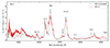 |
Fig. 1. Nebular spectrum of SN 2023ixf at 445 days (red line) compared to the spectrum at 259 days (gray line; F24). The spectra were corrected by extinction and multiplied by respective constant factors to make them match the R-band magnitude at 445 days (see text). The main spectral features are identified by the corresponding ion. |
Photometric BVRI-band data of SN 2023ixf during the nebular phase were obtained from the public database of the American Association of Variable Star Observers (AAVSO)4. The AAVSO database compiles photometry from various, mostly amateur observers around the globe. After rejecting discrepant data points, the resulting light curves contained about 500–700 entries in the BVR bands between approximately 90 and 480 days after the explosion, and 177 entries in the I band between 90 and 390 days. Additional photometry in the gr bands was obtained from the Zwicky Transient Facility (ZTF; Bellm et al. 2019; Masci et al. 2019) via the Automatic Learning for the Rapid Classification of Events broker (ALeRCE; Förster et al. 2021). The ZTF photometry covers approximately the range between 200 and 480 days. The late-time light curves described here are shown in Figure 2.
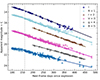 |
Fig. 2. Late-phase light curves of SN 2023ixf. BVRI bands data were downloaded from the AAVSO database. The g and r bands correspond to the ZTF program. The vertical dashed line at 160 days indicates the moment when the slopes increase in the BVRI bands. |
Following F24, we adopted the NASA/IPAC Extragalactic Database5 (NED) redshift of 0.0008 for the host galaxy M101, a distance of 6.85±0.15 Mpc (Riess et al. 2022), a Milky-Way reddening of E(B−V)MW = 0.008 mag (Schlafly & Finkbeiner 2011), and a host-galaxy reddening of E(B−V)Host = 0.031 mag (Lundquist et al. 2023; Zhang et al. 2023). We performed extinction corrections using a total E(B−V)Total = 0.039 mag, and a standard extinction law by Cardelli et al. (1989) with RV = 3.1.
3. Late-time evolution
3.1. Interaction signatures in the spectrum
Figure 1 shows the 445 d spectrum in comparison with that from F24 at 259 d. Both spectra were shifted to the SN rest frame and corrected for extinction using the redshift and extinction values provided in Section 2. We used linear fits to the observed light curves (see Section 3.3) to interpolate the VR-band and extrapolate the I-band magnitudes at 445 d. By comparing these values with synthetic photometry from the spectrum, we found differences of 0.7, 0.8, and 0.8 mag relative to the observed photometry in the V, R, and I bands, respectively. On average, this required a correction of 0.78 mag or a factor of 2.05 to be applied to the 445 d spectrum. Lastly, the 259 d spectrum was scaled down to match the R-band magnitude interpolated at 445 days, as previously described.
We note a general agreement in the line and continuum levels between the spectra, after scaling. However, some differences are evident. First, the flux of the Ca II IR triplet feature is substantially reduced in the later spectrum (see also panel g of Figure 4). This is to be expected, given that the ejecta become increasingly diluted with time and, thus, permitted lines lose strength. We note that a reduction of the Ca II IR triplet feature is seen in the interaction-powered model spectra in comparison with the noninteracting model, as shown by Dessart et al. (2023, see their Figure 4). Therefore, this decrease of the Ca II IR triplet feature may be considered as an indication of ejecta–CSM interaction. The shape of the feature also undergoes some changes, with a notable reduction of the two bluest components relative to the reddest one.
Another distinction emerges in the region blueward of ≈5000 Å, where the later spectrum exhibits an augmented flux level. This is consistent with the observed slower decline of the BV-band light curve in comparison to the declines in the RI bands, as detailed in Section 3.3. An excess in the blue continuum has been identified as an indicator of ejecta-CSM interaction (Dessart & Hillier 2022). Moreover, Dessart et al. (2023) show that the excess flux in the blue range is not attributable to continuum emission but rather to the superposition of an Fe I and Fe II line forest (see their Figure A.3). Nonetheless, a relative brightening in the blue range can also occur due to the presence of a light echo.
Notably, as seen in Figure 1, an excess flux is observed beyond 9000 Å at 445 d, in comparison with the 259 d spectrum. This feature may be interpreted as a flat-topped, blueshifted, broad emission from the Mg II λλ 9218,9244 line that, according to Dessart et al. (2023), may arise as a consequence of ejecta–CSM interaction. Further evidence of the interaction nature of this emission is given in Section 3.2.2, where we analyze the line profile.
The fourth and arguably most remarkable difference is seen in the shape of the Hα line. The new spectrum presents a very complex profile (see Section 3.2.2 for a detailed analysis), wherein the relatively wide profile observed on day 259 (F24) appears to have decreased in flux and shifted further to the blue, while two additional, very wide components flank it on either side. This is possibly another indication of interaction between the SN ejecta and a dense CSM shell (Dessart et al. 2023). Unfortunately, it is not possible to test whether Hβ suffers the same evolution because it is likely embedded in a superposition of mostly Fe I and Fe II lines, as mentioned above.
This type of evolution of the Hα profile has been seen in other SNe II, as well as in some Type IIb SNe, such as SN 1993J (Filippenko et al. 1994; Matheson et al. 2000), and SN 2013df (Maeda et al. 2015). Boxy Hα profiles have been observed in SNe II to appear in otherwise spectroscopically and photometrically normal events, such as SNe 2004et (Kotak et al. 2009), 2007it (Andrews et al. 2011), 2008jb (Prieto et al. 2012), 2013ej (Mauerhan et al. 2017), and 2017eaw (Weil et al. 2020). However, these observations occurred at later epochs (after ≈700 days) than in SN 2023ixf. The lack of spectral coverage at ∼1000 days or after in the majority of events precludes an assessment of whether all SNe II eventually transition to spectra dominated by interaction. Interestingly, other SNe II that showed multiple peaks or boxy emission starting as early as 200–400 days were luminous, linear, or short-plateau events. Some examples are SNe 1979C (Branch et al. 1981), 2007od (Inserra et al. 2011), 2011ja (Andrews et al. 2016), 2013by (Black et al. 2017), 2014G (Terreran et al. 2016), 2017ahn (Tartaglia et al. 2021), 2017gmr (Andrews et al. 2019), 2017ivv (Gutiérrez et al. 2020). With a plateau duration of ≈80 days (Bersten et al. 2024), which is relatively short compared to the distribution of durations among SNe II (Martinez et al. 2024), SN 2023ixf falls well within this last group of early-interacting events.
Figure 3 shows our nebular spectra of SN 2023ixf and some similar events, along with the prototypical Type II-P SN 1999em. Possibly the closest match to the [O I] λλ 6300,6364 and Hα profiles at around 450 days is that of SN 2013by, although the extent of the red wing is larger in SN 2023ixf. Notably, however, the [Ca II] λλ 7291,7324 line is substantially stronger in SN 2023ixf. At the epoch of our previous spectrum (≈260 d), the [Ca II] emission is similarly strong in both SNe, although with a complex profile in SN 2013by, possibly due to an asymmetric ejecta distribution (Black et al. 2017)6. Another similar event, SN 2017ivv, showed a stark reduction in the [Ca II] strength between ≈340 d and ≈500 d.
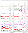 |
Fig. 3. Nebular spectra of SN 2023ixf at 259 and 445 days (blue lines) in comparison to spectra of other SNe II exhibiting interaction signatures at similar ages: SN 2013by (Black et al. 2017), SN 2014G (Terreran et al. 2016), and SN 2017ivv (Gutiérrez et al. 2020). For reference, spectra of the prototypical SN 1999em (Faran et al. 2014) are shown where no widening of the Hα profile was observed. The right panel shows a detail of the Hα profiles as a function of velocity relative to the rest wavelength of 6563 Å. Comparison data were downloaded from the Wiserep (Yaron & Gal-Yam 2012) database (https://www.wiserep.org/) and were not corrected for extinction. |
The spectroscopic evolution of SN 2023ixf between ≈250 d and ≈450 d qualitatively follows what is shown by the radiative transfer models by Dessart et al. (2023). The interaction signatures appear slightly earlier in SN 2023ixf than in the models. From Figure 4 (left panel) of that work it can be seen that the 445 d spectrum presented here is most similar to the model spectrum at 600 d. This phase appears to represent a midpoint in the transition between decay-power dominated and interaction-power dominated spectra. The transition is evident by the simultaneous presence of a narrower, peaked component and a broader, boxy component of Hα (see Section 3.2.2).
3.2. Line profiles
Figure 4 shows the profiles as a function of velocity for the main emission lines in the 259 d and 445 d spectra. Strikingly, the shapes of the [O I] λλ 6300,6364 and [Ca II] λλ 7291,7324 features remain nearly unchanged (see panels c) and f), respectively). The same appears to be the case of the Na I D line (panel b) that exhibits a P-Cygni profile of similar strength at both epochs. The observed change in this feature can be attributed to the continuum level.
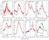 |
Fig. 4. Line profiles as a function of velocity for the main emission features in the spectra of SN 2023ixf at 259 days (gray lines) and 445 days (red lines). Similarly to Figure 1, both spectra were scaled to match the R-band photometry at 445 days. Vertical lines indicate the location of rest (solid) for the reference wavelength of each line, as given below, and in panel d), additionally at velocities of ±8000 km s−1 (dashed). Panel h) shows the region of the Mg II λλ 9218,9244 feature, which is only partly covered, and it includes for reference a reproduction of the Hα profile at 445 days (green line). Reference wavelengths in each panel are: a) 4571 Å, b) 5890 Å, c) 6300 Å, d) 6563 Å, e) 7155 Å, f) 7300 Å, g) 8542 Å, and h) 9231 Å. |
Another feature that suffers little evolution is the bump observed at around 7700 Å (see Figure 1). Its identification is unclear. It may be attributed to O I λ 7774, although the region may be strongly affected by Fe I and Fe II emission lines (Dessart et al. 2023). If this feature were indeed due to O I λ 7774, its profile would differ from that of [O I] λλ 6300,6364, displaying a single peak centered at ≈−3000 km s−1. A possible blueshifted absorption, such as those of P-Cygni profiles, may also be present at both epochs. However, we note that this region may be affected by uncorrected telluric absorption.
At the same time, other lines, such as Mg I] λ 4571 (panel a) and [Fe II] λλ 7155,7171 (panel e), exhibit an increase in flux relative to the continuum. Nevertheless, the shapes of these two features do not evolve substantially, and their peaks show a rather constant blueshift of ≈1000–1200 km s−1. Remarkably, the most obvious changes in the shape of the line profiles are seen in Hα (panel d), Mg II λλ 9218,9244 (panel h), and Ca II λλ 8498,8542,8662 (panel g).
3.2.1. Unchanged [O I] and [Ca II] profiles
The [O I] λλ 6300,6364 feature exhibits a double-peaked profile that can be well represented by two Gaussian components (see Figure 5). Both components have a full width at half maximum (FWHM) of ≈2100 km s−1 and are centered at –1250 and +1500 km −1 relative to the location of the [O I] λ 6300 line. The width and location of these lines are similar to those invoked by F24 to fit the 259 d spectrum. In that previous work, the [O I] fit included two extra narrow (FWHM = 500 km s−1) components that might be present in the 445 d spectrum as well. However, the lower signal-to-noise ratio at 445 days prevents us from confirming this. We also note that no attempt is made in our fitting to reproduce the “bridge” emission seen between [O I] and Hα. An interpretation of such emission will be given below in our analysis of the Hα profile. The lack of evolution in the double-peaked [O I] profile suggests the same asymmetric geometry for the oxygen-rich region of the ejecta as was interpreted by F24.
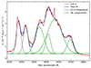 |
Fig. 5. Multicomponent Gaussian fit to the [O I] λλ 6300,6364 and Hα emission complex in the 445 d spectrum of SN 2023ixf (red line). The sum of all six Gaussian components that fits the observations is shown with a blue line. Two components are associated with the [O I] λλ 6300,6364 feature (gray lines), while the other four components reproduce the Hα profile (green lines). See the text for further explanations. |
As shown in Figure 4, the [Ca II] λλ 7291,7324 profile is remarkably similar at 445 and 259 days. Both its equivalent width and the specific structure of peaks and shoulders remain nearly unchanged. This suggests that the same Ca-rich emitting region is observed at both epochs. From a single Gaussian profile fit, we derive a width of FWHM = 4100 km s−1.
3.2.2. The transformation of Hα
The shape of the Hα line is where most of the evolution is seen between 259 and 445 days (see Figure 1). At the earlier epoch, the profile could be interpreted as composed of a broad (FWHM = 5300 km s−1) emission centered at rest plus a narrower (FWHM = 1600 km s−1) component blue-shifted by 1800 km s−1 (F24). At 445 days, there appears to be a central broad emission with a slanted top profile superimposed on an even broader structure with sharp edges. This complex profile can be fit with multiple Gaussian components, as shown in Figure 5. The fit was done simultaneously for Hα and [O I] λλ 6300,6364 due to the blending between both features.
We achieve a reasonable match to the observed Hα profile by invoking four Gaussian components. The number of Gaussians was chosen in order to reproduce the two-Gaussian fit performed by F24 on the 259 d spectrum plus two additional components at larger displacements on each side that reproduce the broader extent of the line. The widest of these components, with FWHM = 6300 km s−1, is centered near the rest wavelength at ≈+150 km s−1. An additional narrower component, with FWHM = 2200 km s−1 and blueshifted by ≈−2200 km s−1, accounts for the peak of the central emission. Both of these central components are slightly wider than those fit to the 259 d spectrum. Lastly, two roughly symmetrical Gaussians centered at –5500 and +5900 km s−1, with widths of FWHM ≈ 3900 and 2700 km s−1, respectively, reproduce the extreme of the wider boxy emission. The Gaussian on the blue extreme has a larger amplitude than its counterpart on the red end. We note that this multicomponent fit is slightly wider than the observations on the blue edge of the Hα profile. This may be due to the presence of an extra emission component in between the [O I] λλ 6300,6364 line and Hα that is not accounted for in the fit. Blending with the [O I] feature may also explain the larger FWHM value found for the bluest Gaussian as compared with that of the reddest component in the Hα fit. In addition, the fit does not reproduce an apparent depression in the spectrum at about 6470 Å. This depression may be due to an absorption component of Hα centered at about –4250 km s−1. A similar feature is noticeable in the 259 d spectrum although at a higher velocity (see panel d of Figure 4).
The two extreme Gaussian components may in principle arise from a bipolar, high-velocity ejecta distribution. However, if we assume them to be powered by 56Co decay, these high-velocity emission components should have been present at phases earlier than 259 days, which is not the case (see also Kumar et al. 2025; Michel et al. 2025). Their late-phase appearance is instead likely associated with the fast SN ejecta encountering preexisting, slowly moving CSM. Under this interpretation, the central components may be dominated by emission from the SN ejecta7, as its width is comparable to that seen at 259 days, whereas the broader boxy component may be the result of interaction between the SN ejecta and a preexisting CSM that started some time between 259 and 445 days. The slanted top of the central component may be due in this scenario to obscuration of the far side of the ejecta, which would explain the reduced flux on the red side of the line and the blueshift of its peak. A similar type of obscuration may affect the red side of the broader component, which is weaker than the blue side. The sharp edges seen on each side at ≈±8000 km s−1 may be produced by the emission from a roughly spherical shell or axisymmetrical structure where the shock front is located.
We note that while Hα exhibits this transformation and its central peak shifts to the blue, the peaks of the other spectral features remain nearly fixed in place (see Figure 4). This may be explained if the obscuration region partially covers the outer H-emission layers, thereby preferentially allowing (blueshifted) photons from the near side of the ejecta to escape (Chugai 1992). Such a phenomenon may occur if the obscuration region resides in a complex, asymmetric, or clumpy structure that might be associated with the ejecta–CSM interaction front. In turn, lines from heavier elements would form deeper in the ejecta where the obscuration zone would equally absorb photons from the near (blueshifted) and far (redshifted) emitting regions thereby keeping their central wavelengths unchanged.
Following the above scenario, we present an alternative representation of the Hα profile as the sum of an underlying boxy component, in the form of a trapezoid, and a blueshifted, more centrally peaked component. Assuming that the red side of the line is affected by absorption, we use only the data blueward of the rest wavelength to produce a fit. The trapezoid is fit to the blue extreme of the profile, i.e., the regions between ≈−4000 and –8000 km s−1. For the peaked component, we fit the data from 0 to ≈−4000 km s−1 using two half-Gaussians, one in emission and one in absorption. The choice of a Gaussian shape for the absorption component is arbitrary and it was made for simplicity. We noted that the central Gaussian was poorly constrained given the relatively narrow and steep profile. Therefore, we fixed the amplitude of the positive Gaussian to match that of the Hα emission in the scaled-down 259 d spectrum, assuming a similar origin for the feature.
Figure 6 shows the result of simultaneously fitting the trapezoid and the positive and negative Gaussians to the blue side of the Hα line. No attempt was made to reproduce the dip at ≈6470 Å mentioned above. The dotted lines in the Figure show the three individual fit components mirrored toward the red side of the line. It is worth noting that the edge of the trapezoid that was fit on the blue extreme of the line matches very well the red edge, which provides support to its interpretation as the emission from a symmetrical interaction region.
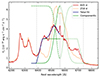 |
Fig. 6. Simulated interaction-powered (trapezoid) plus radioactive-powered (Gaussian) fit to the blue side of the Hα profile in the 445 d spectrum of SN 2023ixf (red line). The total fitted profile is shown with a blue line. Green lines show the individual fit components: trapezoid and emission Gaussian in solid lines, and absorption Gaussian in dashed lines. Dotted green lines indicate the symmetrical extension of each component toward the red half of the profile. Note that the trapezoid matches the observed red edge of the line well. Vertical gray lines indicate the location of rest (solid) and ±8000 km s−1 (dashed). The scaled-down 259 d spectrum of SN 2023ixf (orange line, F24) was used to fix the amplitude of the emission Gaussian. See the text for further details. |
Within this representation we can derive a total unattenuated flux of the interaction-powered Hα emission as the integrated flux of the trapezoid mirrored around the rest wavelength. Adopting the distance to M101 given in Section 2 this gives a luminosity of 4.2×1038 erg s−1. This value is slightly higher than that of SN 2017eaw at 900 days, and about one order of magnitude larger than what was measured on SN 2004et and SN 2013ej at similar ages when they were undergoing interaction (see Weil et al. 2020). Similar Hα interaction-driven luminosities of ∼1038 erg s−1 were found for the Type IIb SN 1993J at 367 d (Patat et al. 1995), and SN 2013df at 626 d (Maeda et al. 2015).
The unattenuated Hα luminosity due to the ejecta in turn can be considered as that of the emission Gaussian, which is 3.0×1038 erg s−1. This value is also comparable with those of noninteracting SNe II at a similar age (Weil et al. 2020). However, this assumed radioactive-powered Hα luminosity is not well-constrained for SN 2023ixf because we fixed the line strength based on the scaled-down 259 d spectrum.
Panel h) of Figure 4 depicts the profile evolution of the feature we identified as Mg II λλ 9218,9244. Unfortunately, the profile is not completely covered. However, the blue side exhibits a “boxy” profile, similar to that of Hα, extending to ≈−8000 Å. The top of the emission appears slanted toward the blue side, also in agreement with the Hα profile. If this identification is correct, it suggests that Mg II is the species that most closely follows the behavior of the interaction-driven Hα emission.
It is interesting to examine the evolution of the region in between Hα and the [O I] feature at around 6400 Å. At 259 days the spectrum exhibits a peak centered at 6412 Å that is not usually seen in SN-II spectra (Silverman et al. 2017). F24 suggested this emission could be due to Fe II λ 6456 or O I λ 6456 blueshifted by ≈−2000 km s−1. A similar feature appeared in the spectra of SN 2014G between 100 and 190 days that was possibly identified as high-velocity Hα by Terreran et al. (2016). If the identification is correct, the velocity of the emission peak evolved in that SN from ≈−7600 to ≈−6800 km s−1 during the time that it was detected. We further notice a similar emission feature centered at ≈−7000 km s−1 in the spectra of SN 2017ivv between 242 and 285 days (Gutiérrez et al. 2020), much alike the case of SN 2023ixf. Interestingly, as can be appreciated in Figure 4, the location of the peak at 259 days roughly matches the blue edge of the boxy Hα line at 445 days. Blueward of the emission peak, the spectrum shape remains unchanged between the two epochs. This may indicate a common origin for both features, which would support the H identification of the peak seen at 259 days.
It is unclear whether this possible H feature is related with high-velocity “cachito” absorption features commonly observed during the plateau phase (Gutiérrez et al. 2017), which have been attributed to interaction between the SN ejecta and the RSG progenitor's wind (Chugai et al. 2007). High-velocity components of Hα and Hβ were seen in SN 2023ixf during the plateau phase (Singh et al. 2024), although the authors discuss that they are more likely due to an asymmetric ejecta rather than to CSM interaction. According to the radiation transfer calculations of SNe II with CSM interaction by Dessart & Hillier (2022) and Dessart et al. (2023), this type of absorption is persistent well into the nebular phase. However, we cannot identify it in the late-time spectra of SN 2023ixf.
We can compute the internal radius of a putative CSM shell (or distance to the CSM structure) by assuming the SN ejecta traveling at the maximum speed of 8000 km s−1 given by the Hα profile, and the interaction starting at some time between 259 and 445 days since the explosion. This gives a inner radius in the range of 1.8−3.0×1016 cm. Assuming that the CSM shell was produced by a wind expelled from the RSG progenitor at a velocity of ∼10 km s−1, then this material must have been lost from the star up until ∼500−1000 years prior to the SN event. If we consider the emission peak seen at ≈6400 Å in the 259 d spectrum as due to CSM interaction, then the lowest radius and age values above are to be taken as upper limits.
3.3. Light-curve decline
The extra power released by the ejecta–CSM interaction can produce a flattening of the light curves. This effect has been observed as a break in the decline slopes for a number of SNe II following the appearance of the boxy Hα profiles. Notably, the break occurred earlier (before 500 d) in SN 2007od (Andrews et al. 2010; Inserra et al. 2011), SN 2011ja (Andrews et al. 2016), and SN 2017ivv (Gutiérrez et al. 2020) than in SN 2004et (after 600 d; Maguire et al. 2010), SN 2013ej (possibly after 750 d; Mauerhan et al. 2017)8, and SN 2017eaw (after 700 d; Weil et al. 2020), roughly matching the timing of the spectral interaction signatures (see Section 3.1). This supports the association of both spectroscopic and photometric effects to the same physical cause, most probably CSM interaction. Lack of sufficient coverage in the light curves of other SNe II with interaction signatures in the spectra prevents us from drawing a strong general conclusion about this association. In addition, we note that Andrews et al. (2010) suggested the flattening of the light curves in SN 2007od was due to a light echo from dust that in turn obscured the far side of the ejecta, causing asymmetric line profiles in the late spectra.
Figure 2 shows the late-time optical light curves of SN 2023ixf (see Section 2) between ≈100 and ≈480 days. During this time there is no evidence of a decrease in the decline rates. Moreover, Michel et al. (2025) found no apparent break in the late-time optical light curves until ≈520 d, with the possible exception of the I and z bands, which the authors suggest are associated with emission from preexisting or newly formed dust.
Since the onset of the radioactive tail at ≈90 days, the BVRI light curves show a relatively slow decline until ≈160 days (dashed line in Figure 2). After that, the slopes increase and remain roughly constant in all bands until the end of the coverage (≈480 days in BVR, and ≈390 days in I band). We performed linear fits to the photometric data during both epoch ranges. In the range of 90–160 d, the slopes are 0.51±0.06, 1.11±0.04, 1.01±0.13, and 1.12±0.09 mag (100 d)−1 in BVRI, respectively. At times later than 160 d, the slopes in the same bands are 0.95±0.06, 1.28±0.04, 1.39±0.03, 1.56±0.01 mag (100 d)−1. Note that the increase in decline slope after 160 d is substantially larger in B band than in VRI. In addition, during both time regimes, the decline slopes are the larger the longer the filter's wavelength. The same is seen in the gr-band light curves from ZTF that cover the range of 200–444 days. The slopes are 1.06±0.01 and 1.39±0.03 mag (100 d)−1 in g and r, respectively. The lack of change in slopes between ≈200 and ≈500 days indicates that if CSM interaction were responsible for the spectral evolution described in Sections 3.1 and 3.2.2, it would not be strong enough to produce a notable change in the light curves, at least during the time covered by the data.
Except in the B band, the decline rates calculated above are larger than the rate of 0.98 mag (100 d)−1 that is expected from the radioactive decay of 56Co. This has been commonly seen in SNe II by Anderson et al. (2014), who derived an average V-band decline rate during the radioactive tail of 1.47±0.82 mag (100 d)−1. Furthermore, the authors note that SNe II with steeper V-band declines during the plateau phase tend to show larger decline rates during the radioactive tail. Note also that Bersten et al. (2024) measured larger than average decline rates in the bolometric light curve of SN 2023ixf both during the plateau and the radioactive tail. Similarly steep declines have been measured at 200–400 days in other SNe II with signs of interaction in the spectra at relatively early times during the nebular phase, namely SN 2013by (Black et al. 2017), SN 2014G (Terreran et al. 2016), and SN 2017ivv (Gutiérrez et al. 2020), as well as in other objects with later signs of interaction in the spectra, such as SN 2004et (Maguire et al. 2010), SN 2008jb (Prieto et al. 2012), SN 2013ej (Dhungana et al. 2016), and SN 2017eaw (Buta & Keel 2019).
Assuming the late-time light curve is powered solely by radioactive decay, the deviation from the expected decline rate can be due to incomplete gamma-ray trapping in the ejecta or to increased extinction by newly formed dust, or a combination of both. Dust extinction should, however, produce systematically steeper light curves in the bluer bands, which is contrary to what was observed.
4. Progenitor mass revisited
Nebular spectroscopy can be used to estimate the initial mass of the progenitor. One way to do this is by deriving the mass of oxygen in the ejecta and linking that mass with oxygen yields from explosion models of stars with different initial masses. The mass of neutral oxygen can be determined from the flux of the [O I] λλ 6300,6364 line, provided that the temperature of the emitting gas is known (Uomoto 1986; Jerkstrand et al. 2014). This O I mass is in principle a lower limit to the total oxygen mass in the ejecta, bearing the fraction of ionized oxygen (Kuncarayakti et al. 2015). The temperature can be estimated by measuring the flux ratio of [O I] λ 5577 to [O I] λλ 6300,6364 (see Equation (2) in Jerkstrand et al. 2014). However, [O I] λ 5577 is a weak line and in many cases it is lost in the noise. Moreover, the dependence of the O I mass on temperature is through an exponential, which makes it very sensitive to uncertainties in the temperature (see Elmhamdi et al. 2004).
F24 placed a lower limit on the [O I] λ 5577 flux in the 259 d spectrum of SN 2023ixf, and thereby derived a lower limit for the temperature of 3700 K. Based on the [O I] λλ 6300,6364 flux of 2.38×10⁻¹³ erg s−1 cm−2 measured on the 259 d spectrum, the authors found an O I mass of ≈0.5 M⊙. The [O I] λλ 6300,6364 flux at 445 days can be obtained from the Gaussian fits described in Section 3.2.1. The result is 1.2×10⁻¹⁴ erg s−1 cm−2, i.e., 20 times smaller than that at 259 days. The [O I] λ 5577 line is undetectable at 445 days, which prevents a temperature estimate from being obtained. Assuming a temperature of 3330 K measured from the 451 d spectrum of SN 2012aw by Jerkstrand et al. (2014), the resulting O I mass from the 445 d spectrum of SN 2023ixf would be 0.05 M⊙. This is a factor of ten lower than the mass derived from the 259 d spectrum. In order to recover the same O I mass at 445 days as at 259 days, and assuming all other physical conditions remain constant, the required temperature at 445 days would be ≈2500 K. Given the number of assumptions and the critical dependence on temperature involved in this method, we move on to directly compare the observed spectrum with synthetic models.
Figure 7 shows the 445 d spectrum of SN 2023ixf in comparison with a series of SN II synthetic spectra of varying progenitor masses calculated by Dessart et al. (2021) for an age of 350 days. Similarly, Figure 8 presents a comparison with the models at 450 days computed by Jerkstrand et al. (2014, 2018). In both comparisons, the model spectra do not include any effect of CSM interactions. Therefore, the Hα line and the region below ≈5500 Å are not expected to match the observations. Instead, we focus the comparison on the [O I] λλ 6300,6364 and [Ca II] λλ 7291,7324 emissions, which have been used as indicators of the initial mass of the progenitor (e.g., see Fransson & Chevalier 1989; Dessart et al. 2021), and are relatively free from interaction effects, as shown by Dessart et al. (2023). The synthetic spectra are scaled to match the average flux of the photometry-corrected spectrum (see Section 3.1) in the range of 6800–8200 Å, i.e., within most of the i′ and I bands. Therefore, the scaling factor is dominated by the [Ca II] λλ 7291,7324 line flux. This choice of scaling factor, rather than using the distance, age, and 56Ni mass, is made to account for differences in the fraction of γ-ray escape from the ejecta between models and observation. The comparison indicates that the observed spectrum is best matched by models with initial masses between 10 and 15 M⊙ from Dessart et al. (2021), and between 12 and 15 M⊙ from Jerkstrand et al. (2014). Models with MZAMS = 9 M⊙ exhibit comparatively narrow emission lines that do not match the observations. On the other hand, for MZAMS≥19 M⊙ the [O I] λλ 6300,6364 emission becomes too strong in both sets of model spectra.
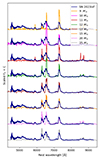 |
Fig. 7. The spectrum of SN 2023ixf at 445 days (blue lines) in comparison to radiative transfer calculations at an age of 360 days performed by Dessart et al. (2021) for various SN II progenitors of different masses (colored lines as labeled). The model spectra were normalized to match the observed flux integrated between 6900 and 8200 Å. |
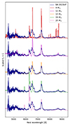 |
Fig. 8. Similar to Figure 7, but for the 445 d spectrum (blue lines), compared to radiative transfer calculations of SN II spectra at 450 days for progenitors of various initial masses (colored lines as labeled). Models for 9 M⊙ are from Jerkstrand et al. (2018), while models for the other masses are from Jerkstrand et al. (2014). The model spectra were normalized to match the observed flux integrated between 6900 and 8200 Å. |
A more quantitative comparison can be done using the flux ratios of [O I] λλ 6300,6364 over [Ca II] λλ 7291,7324. Figure 9 shows the ratios computed from both series of synthetic spectra mentioned above. From the observed spectrum, we obtain a ratio of 0.55, which is in agreement with that of 0.51 obtained from the 259 d spectrum by F24. This stability of the oxygen to calcium ratio has been observed in other SNe II and in core-collapse SNe in general (e.g., see Elmhamdi 2011; Maguire et al. 2012), which provides support to the method. From Figure 9, we can conclude that SN 2023ixf is compatible with models with initial masses between 10 and 15 M⊙.
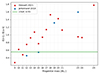 |
Fig. 9. Flux ratio of the [O I] λλ 6300,6364 line to the [Ca II] λλ 7294,7321 line as measured in the 445 d spectrum of SN 2023ixf (horizontal green line) in comparison to the ratios measured based on the model spectra of various progenitor masses from Dessart et al. (2021) (red circles) and Jerkstrand et al. (2014) (blue circles). This comparison favors a progenitor mass in the range of about 10–15 M⊙. |
The present analysis favors a mass of the progenitor for SN 2023ixf on the low range among those derived from the analysis of the pre-explosion imaging (see Section 1). This is in agreement with the study of the 259 d spectrum by F24, and with the hydrodynamical modeling of the light curves and expansion velocities during the plateau phase by Bersten et al. (2024) and Moriya & Singh (2024).
5. Conclusions
We have presented a second nebular spectrum of SN 2023ixf obtained with GMOS-N at 445 days after the explosion. In the approximately 180 days since our previous spectrum (presented in F24), the SN underwent a dramatic transformation. The new spectrum shows clear indications of ejecta–CSM interaction, most notably in the appearance of a boxy emission component of the Hα line that may also be present in the Mg II λλ 9218,9244 line (see Figure 4). This suggests that the ejecta encountered a CSM shell. The flux in the region blueward of ≈5000 Å shows a relative enhancement, which has also been indicated as a sign of CSM interaction (Dessart & Hillier 2022). This transformation seen at 445 days9 places SN 2023ixf within the group of SNe II that have shown interaction signatures in their nebular spectra before ≈500 days. This group appears to be composed of SNe with either short plateaus or linear light curves.
The boxy Hα component extends to ±8000 km s−1. Assuming this expansion velocity for the SN ejecta, an age of 445 days corresponds to a distance of ≈3×1016 cm for the putative CSM shell (or axisymmetric structure) from the progenitor star. This is an upper limit since the interaction may have started as early as ≈260 days (see Section 3.2). In conclusion, the CSM must have been located at a distance of ∼1016 cm. Assuming a standard wind velocity of ∼10 km s−1 for the RSG progenitor, the material should have been expelled by the star up until ≈500−1000 years before the explosion. We note that, contrary to what was observed in other interacting SNe II, in SN 2023ixf the appearance of the boxy Hα profile was not accompanied by a flattening of the light curves at least until ≈500 days, as is expected due to the release of extra interaction power (Dessart et al. 2023). However, it is still possible that this phenomenon may be detected at even later times.
Some of the main emission lines in the 445 d spectrum, such as [O I] λλ 6300,6364, [Ca II] λλ 7291,7324, Na I D, and [Fe II] λλ 7155,7171, exhibited remarkably similar profiles compared to their counterparts at 259 days (see Figure 4). Assuming these features continued to be dominated by emission from the SN ejecta and not from the interaction region, this indicates that the geometry of the emitting regions of the ejecta was not substantially modified during the time elapsed between the observations.
Moreover, the fact that the [O I] λλ 6300,6364 and [Ca II] λλ 7291,7324 lines remain apparently unaffected by the CSM interaction allowed us to derive an updated estimate of the progenitor mass. This was obtained by comparison with synthetic nebular spectra calculated by Jerkstrand et al. (2014, 2018), and Dessart et al. (2021) for noninteracting SNe II of various progenitor masses. The results (see Figures 7, 8, and 9) favor a progenitor mass of MZAMS≈10−15 M⊙, similar to what was concluded by F24 using the 259 d spectrum. We note, however, that the synthetic spectra were computed assuming progenitors with standard mass-loss prescriptions. Alternatively, the progenitor may have been a star with a slightly higher initial mass but that underwent enhanced mass loss, as proposed by Fang et al. (2025).
The proximity of SN 2023ixf provides a rare opportunity to monitor the evolution of this event over the coming years or even decades. Future observations may reveal further details of the CSM properties and the possible formation of dust in the ejecta–CSM interface. This will provide important clues about the evolution of massive stars and specifically their mass-loss processes.
Acknowledgments
We are thankful to Jennifer Andrews for her willingness to share data and information, and to the Gemini Observatory for encouraging fluid group interaction between the Program GN-2024A-Q-139 and Program GN-2024A-Q-309 teams. H.K. was funded by the Research Council of Finland projects 324504, 328898, and 353019. K.M. acknowledges support from JSPS KAKENHI grants JP24H01810 and JP24KK0070. K.M. and H.K. are partly supported by the JSPS bilateral program between Japan and Finland (JPJSBP120229923). Based on observations obtained at the international Gemini Observatory (GN-2024A-Q-309, PI: Ferrari), a program of NSF's NOIRLab, which is managed by the Association of Universities for Research in Astronomy (AURA) under a cooperative agreement with the National Science Foundation. On behalf of the Gemini Observatory partnership: the National Science Foundation (United States), National Research Council (Canada), Agencia Nacional de Investigación y Desarrollo (Chile), Ministerio de Ciencia, Tecnología e Innovación (Argentina), Ministério da Ciência, Tecnologia, Inovações e Comunicações (Brazil), and Korea Astronomy and Space Science Institute (Republic of Korea). This work was made possible by observations from the Gemini North telescope, located within the Maunakea Science Reserve and adjacent to the summit of Maunakea. We are grateful for the privilege of observing the Universe from a place that is unique in both its astronomical quality and its cultural significance. We acknowledge with thanks the variable star observations from the AAVSO International Database contributed by observers worldwide and used in this research.
That is, usually broad emission exhibiting sharp, roughly symmetrical edges.
Where the authors specifically excluded linear SNe II.
Excluding the estimate of MZAMS = 8−10 M⊙ by Pledger & Shara (2023) that neglects the presence of dust.
Note that there can be contamination from adjacent [Fe II] and [Ni II] lines.
Note, however, that this central emission may also be affected by interaction with an asymmetric CSM (see Kumar et al. 2025).
Note, however, that Dhungana et al. (2016) find a break in the light curves of SN 2013ej at ≈180 days.
Note that Kumar et al. (2025) notices a similar boxy Hα profile at 363 days.
References
- Anderson, J. P., González-Gaitán, S., Hamuy, M., et al. 2014, ApJ, 786, 67 [Google Scholar]
- Andrews, J. E., Gallagher, J. S., Clayton, G. C., et al. 2010, ApJ, 715, 541 [Google Scholar]
- Andrews, J. E., Sugerman, B. E. K., Clayton, G. C., et al. 2011, ApJ, 731, 47 [NASA ADS] [CrossRef] [Google Scholar]
- Andrews, J. E., Krafton, K. M., Clayton, G. C., et al. 2016, MNRAS, 457, 3241 [NASA ADS] [CrossRef] [Google Scholar]
- Andrews, J. E., Sand, D. J., Valenti, S., et al. 2019, ApJ, 885, 43 [Google Scholar]
- Beasor, E. R., Davies, B., Smith, N., et al. 2020, MNRAS, 492, 5994 [Google Scholar]
- Bellm, E. C., Kulkarni, S. R., Graham, M. J., et al. 2019, PASP, 131, 018002 [Google Scholar]
- Berger, E., Keating, G. K., Margutti, R., et al. 2023, ApJ, 951, L31 [NASA ADS] [CrossRef] [Google Scholar]
- Bersten, M. C., Orellana, M., Folatelli, G., et al. 2024, A&A, 681, L18 [NASA ADS] [CrossRef] [EDP Sciences] [Google Scholar]
- Black, C. S., Milisavljevic, D., Margutti, R., et al. 2017, ApJ, 848, 5 [NASA ADS] [CrossRef] [Google Scholar]
- Bostroem, K. A., Pearson, J., Shrestha, M., et al. 2023, ApJ, 956, L5 [NASA ADS] [CrossRef] [Google Scholar]
- Bostroem, K. A., Sand, D. J., Dessart, L., et al. 2024, ApJ, 973, L47 [NASA ADS] [CrossRef] [Google Scholar]
- Branch, D., Falk, S. W., McCall, M. L., et al. 1981, ApJ, 244, 780 [Google Scholar]
- Bruch, R. J., Gal-Yam, A., Yaron, O., et al. 2023, ApJ, 952, 119 [NASA ADS] [CrossRef] [Google Scholar]
- Buta, R. J., & Keel, W. C. 2019, MNRAS, 487, 832 [NASA ADS] [CrossRef] [Google Scholar]
- Cardelli, J. A., Clayton, G. C., & Mathis, J. S. 1989, ApJ, 345, 245 [Google Scholar]
- Chandra, P., Chevalier, R. A., Maeda, K., Ray, A. K., & Nayana, A. J. 2024, ApJ, 963, L4 [NASA ADS] [CrossRef] [Google Scholar]
- Chevalier, R. A., & Fransson, C. 2017, in Handbook of Supernovae, eds. A. W. Alsabti, & P. Murdin, 875 [Google Scholar]
- Chugai, N. N. 1992, Soviet. Astron. Lett., 18, 239 [Google Scholar]
- Chugai, N. N., Chevalier, R. A., & Utrobin, V. P. 2007, ApJ, 662, 1136 [NASA ADS] [CrossRef] [Google Scholar]
- Dessart, L., & Hillier, D. J. 2022, A&A, 660, L9 [NASA ADS] [CrossRef] [EDP Sciences] [Google Scholar]
- Dessart, L., Hillier, D. J., Sukhbold, T., Woosley, S. E., & Janka, H. T. 2021, A&A, 652, A64 [NASA ADS] [CrossRef] [EDP Sciences] [Google Scholar]
- Dessart, L., Gutiérrez, C. P., Kuncarayakti, H., Fox, O. D., & Filippenko, A. V. 2023, A&A, 675, A33 [NASA ADS] [CrossRef] [EDP Sciences] [Google Scholar]
- Dhungana, G., Kehoe, R., Vinko, J., et al. 2016, ApJ, 822, 6 [NASA ADS] [CrossRef] [Google Scholar]
- Dong, Y., Sand, D. J., Valenti, S., et al. 2023, ApJ, 957, 28 [NASA ADS] [CrossRef] [Google Scholar]
- Elmhamdi, A. 2011, Acta Astron., 61, 179 [NASA ADS] [Google Scholar]
- Elmhamdi, A., Danziger, I. J., Cappellaro, E., et al. 2004, A&A, 426, 963 [NASA ADS] [CrossRef] [EDP Sciences] [Google Scholar]
- Fang, Q., Moriya, T. J., Ferrari, L., et al. 2025, ApJ, 978, 36 [NASA ADS] [CrossRef] [Google Scholar]
- Faran, T., Poznanski, D., Filippenko, A. V., et al. 2014, MNRAS, 442, 844 [NASA ADS] [CrossRef] [Google Scholar]
- Ferrari, L., Folatelli, G., Ertini, K., Kuncarayakti, H., & Andrews, J. E. 2024, A&A, 687, L20 [NASA ADS] [CrossRef] [EDP Sciences] [Google Scholar]
- Filippenko, A. V., Matheson, T., & Barth, A. J. 1994, AJ, 108, 2220 [NASA ADS] [CrossRef] [Google Scholar]
- Förster, F., Moriya, T. J., Maureira, J. C., et al. 2018, Nat. Astron., 2, 808 [CrossRef] [Google Scholar]
- Förster, F., Cabrera-Vives, G., Castillo-Navarrete, E., et al. 2021, AJ, 161, 242 [CrossRef] [Google Scholar]
- Fransson, C., & Chevalier, R. A. 1987, ApJ, 322, L15 [NASA ADS] [CrossRef] [Google Scholar]
- Fransson, C., & Chevalier, R. A. 1989, ApJ, 343, 323 [NASA ADS] [CrossRef] [Google Scholar]
- Grefenstette, B. W., Brightman, M., Earnshaw, H. P., Harrison, F. A., & Margutti, R. 2023, ApJ, 952, L3 [NASA ADS] [CrossRef] [Google Scholar]
- Gutiérrez, C. P., Anderson, J. P., Hamuy, M., et al. 2017, ApJ, 850, 89 [CrossRef] [Google Scholar]
- Gutiérrez, C. P., Pastorello, A., Jerkstrand, A., et al. 2020, MNRAS, 499, 974 [CrossRef] [Google Scholar]
- Hiramatsu, D., Tsuna, D., Berger, E., et al. 2023, ApJ, 955, L8 [NASA ADS] [CrossRef] [Google Scholar]
- Hook, I. M., Jørgensen, I., Allington-Smith, J. R., et al. 2004, PASP, 116, 425 [NASA ADS] [CrossRef] [Google Scholar]
- Hosseinzadeh, G., Farah, J., Shrestha, M., et al. 2023, ApJ, 953, L16 [NASA ADS] [CrossRef] [Google Scholar]
- Inserra, C., Turatto, M., Pastorello, A., et al. 2011, MNRAS, 417, 261 [Google Scholar]
- Iwata, Y., Akimoto, M., Matsuoka, T., et al. 2025, ApJ, 978, 138 [Google Scholar]
- Jacobson-Galán, W. V., Dessart, L., Margutti, R., et al. 2023, ApJ, 954, L42 [CrossRef] [Google Scholar]
- Jacobson-Galán, W. V., Dessart, L., Davis, K. W., et al. 2024, ApJ, 970, 189 [CrossRef] [Google Scholar]
- Jencson, J. E., Pearson, J., Beasor, E. R., et al. 2023, ApJ, 952, L30 [NASA ADS] [CrossRef] [Google Scholar]
- Jerkstrand, A., Fransson, C., Maguire, K., et al. 2012, A&A, 546, A28 [NASA ADS] [CrossRef] [EDP Sciences] [Google Scholar]
- Jerkstrand, A., Smartt, S. J., Fraser, M., et al. 2014, MNRAS, 439, 3694 [Google Scholar]
- Jerkstrand, A., Ertl, T., Janka, H. T., et al. 2018, MNRAS, 475, 277 [Google Scholar]
- Kilpatrick, C. D., Foley, R. J., Jacobson-Galán, W. V., et al. 2023, ApJ, 952, L23 [NASA ADS] [CrossRef] [Google Scholar]
- Kotak, R., Meikle, W. P. S., Farrah, D., et al. 2009, ApJ, 704, 306 [NASA ADS] [CrossRef] [Google Scholar]
- Kumar, A., Dastidar, R., Maund, J. R., Singleton, A. J., & Sun, N. -C. 2025, MNRAS, 538, 659 [Google Scholar]
- Kuncarayakti, H., Maeda, K., Bersten, M. C., et al. 2015, A&A, 579, A95 [CrossRef] [EDP Sciences] [Google Scholar]
- Labrie, K., Simpson, C., Cardenes, R., et al. 2023, Res. Notes Am. Astron. Soc., 7, 214 [Google Scholar]
- Li, G., Hu, M., Li, W., et al. 2024, Nature, 627, 754 [NASA ADS] [CrossRef] [Google Scholar]
- Li, G., Wang, X., Yang, Y., et al. 2025, A&A, submitted [arXiv:2504.03856] [Google Scholar]
- Liu, C., Chen, X., Er, X., et al. 2023, ApJ, 958, L37 [NASA ADS] [CrossRef] [Google Scholar]
- Lundquist, M., O’Meara, J., & Walawender, J. 2023, TNSAN, 160, 1 [NASA ADS] [Google Scholar]
- Maeda, K., Hattori, T., Milisavljevic, D., et al. 2015, ApJ, 807, 35 [NASA ADS] [CrossRef] [Google Scholar]
- Maguire, K., Di Carlo, E., Smartt, S. J., et al. 2010, MNRAS, 404, 981 [NASA ADS] [CrossRef] [Google Scholar]
- Maguire, K., Jerkstrand, A., Smartt, S. J., et al. 2012, MNRAS, 420, 3451 [Google Scholar]
- Martinez, L., Bersten, M. C., Folatelli, G., Orellana, M., & Ertini, K. 2024, A&A, 683, A154 [NASA ADS] [CrossRef] [EDP Sciences] [Google Scholar]
- Masci, F. J., Laher, R. R., Rusholme, B., et al. 2019, PASP, 131, 018003 [Google Scholar]
- Matheson, T., Filippenko, A. V., Ho, L. C., Barth, A. J., & Leonard, D. C. 2000, AJ, 120, 1499 [NASA ADS] [CrossRef] [Google Scholar]
- Matsuoka, T., Maeda, K., Lee, S. -H., & Yasuda, H. 2019, ApJ, 885, 41 [Google Scholar]
- Mauerhan, J. C., Van Dyk, S. D., Johansson, J., et al. 2017, ApJ, 834, 118 [Google Scholar]
- Michel, P. D., Mazzali, P. A., Perley, D. A., Hinds, K. R., & Wise, J. L. 2025, MNRAS, 539, 633 [Google Scholar]
- Moriya, T. J. 2021, MNRAS, 503, L28 [Google Scholar]
- Moriya, T. J., & Singh, A. 2024, PASJ, 76, 1050 [NASA ADS] [CrossRef] [Google Scholar]
- Moriya, T. J., Yoon, S. -C., Gräfener, G., & Blinnikov, S. I. 2017, MNRAS, 469, L108 [NASA ADS] [CrossRef] [Google Scholar]
- Moriya, T. J., Förster, F., Yoon, S. -C., Gräfener, G., & Blinnikov, S. I. 2018, MNRAS, 476, 2840 [Google Scholar]
- Moriya, T. J., Subrayan, B. M., Milisavljevic, D., & Blinnikov, S. I. 2023, PASJ, 75, 634 [NASA ADS] [CrossRef] [Google Scholar]
- Neustadt, J. M. M., Kochanek, C. S., & Smith, M. R. 2024, MNRAS, 527, 5366 [Google Scholar]
- Niu, Z., Sun, N. -C., Maund, J. R., et al. 2023, ApJ, 955, L15 [NASA ADS] [CrossRef] [Google Scholar]
- Patat, F., Chugai, N., & Mazzali, P. A. 1995, A&A, 299, 715 [NASA ADS] [Google Scholar]
- Pledger, J. L., & Shara, M. M. 2023, ApJ, 953, L14 [NASA ADS] [CrossRef] [Google Scholar]
- Prieto, J. L., Lee, J. C., Drake, A. J., et al. 2012, ApJ, 745, 70 [Google Scholar]
- Qin, Y. -J., Zhang, K., Bloom, J., et al. 2024, MNRAS, 534, 271 [NASA ADS] [CrossRef] [Google Scholar]
- Ransome, C. L., Villar, V. A., Tartaglia, A., et al. 2024, ApJ, 965, 93 [CrossRef] [Google Scholar]
- Riess, A. G., Yuan, W., Macri, L. M., et al. 2022, ApJ, 934, L7 [NASA ADS] [CrossRef] [Google Scholar]
- Schlafly, E. F., & Finkbeiner, D. P. 2011, ApJ, 737, 103 [Google Scholar]
- Silverman, J. M., Pickett, S., Wheeler, J. C., et al. 2017, MNRAS, 467, 369 [NASA ADS] [Google Scholar]
- Singh, A., Teja, R. S., Moriya, T. J., et al. 2024, ApJ, 975, 132 [CrossRef] [Google Scholar]
- Smartt, S. J. 2015, PASA, 32, e016 [NASA ADS] [CrossRef] [Google Scholar]
- Smartt, S. J., Eldridge, J. J., Crockett, R. M., & Maund, J. R. 2009, MNRAS, 395, 1409 [CrossRef] [Google Scholar]
- Smith, N. 2014, ARA&A, 52, 487 [NASA ADS] [CrossRef] [Google Scholar]
- Soraisam, M. D., Szalai, T., Van Dyk, S. D., et al. 2023, ApJ, 957, 64 [NASA ADS] [CrossRef] [Google Scholar]
- Tartaglia, L., Sand, D. J., Groh, J. H., et al. 2021, ApJ, 907, 52 [NASA ADS] [CrossRef] [Google Scholar]
- Teja, R. S., Singh, A., Basu, J., et al. 2023, ApJ, 954, L12 [NASA ADS] [CrossRef] [Google Scholar]
- Terreran, G., Jerkstrand, A., Benetti, S., et al. 2016, MNRAS, 462, 137 [Google Scholar]
- Uomoto, A. 1986, ApJ, 310, L35 [NASA ADS] [CrossRef] [Google Scholar]
- Van Dyk, S. D., Cenko, S. B., Poznanski, D., et al. 2012, ApJ, 756, 131 [NASA ADS] [CrossRef] [Google Scholar]
- Van Dyk, S. D., Srinivasan, S., Andrews, J. E., et al. 2024, ApJ, 968, 27 [NASA ADS] [CrossRef] [Google Scholar]
- Vink, J. S., de Koter, A., & Lamers, H. J. G. L. M. 2001, A&A, 369, 574 [NASA ADS] [CrossRef] [EDP Sciences] [Google Scholar]
- Weil, K. E., Fesen, R. A., Patnaude, D. J., & Milisavljevic, D. 2020, ApJ, 900, 11 [Google Scholar]
- Xiang, D., Mo, J., Wang, L., et al. 2024, Sci. China: Phys. Mech. Astron., 67, 219514 [NASA ADS] [CrossRef] [Google Scholar]
- Yaron, O., & Gal-Yam, A. 2012, PASP, 124, 668 [Google Scholar]
- Yaron, O., Perley, D. A., Gal-Yam, A., et al. 2017, Nat. Phys., 13, 510 [NASA ADS] [CrossRef] [Google Scholar]
- Zhang, J., Lin, H., Wang, X., et al. 2023, Sci. Bull., 68, 2548 [NASA ADS] [CrossRef] [Google Scholar]
- Zheng, W., Dessart, L., Filippenko, A. V., et al. 2025, AAS, submitted [arXiv:2503.13974] [Google Scholar]
- Zimmerman, E. A., Irani, I., Chen, P., et al. 2024, Nature, 627, 759 [Google Scholar]
All Figures
|
Fig. 1. Nebular spectrum of SN 2023ixf at 445 days (red line) compared to the spectrum at 259 days (gray line; F24). The spectra were corrected by extinction and multiplied by respective constant factors to make them match the R-band magnitude at 445 days (see text). The main spectral features are identified by the corresponding ion. |
| In the text | |
|
Fig. 2. Late-phase light curves of SN 2023ixf. BVRI bands data were downloaded from the AAVSO database. The g and r bands correspond to the ZTF program. The vertical dashed line at 160 days indicates the moment when the slopes increase in the BVRI bands. |
| In the text | |
|
Fig. 3. Nebular spectra of SN 2023ixf at 259 and 445 days (blue lines) in comparison to spectra of other SNe II exhibiting interaction signatures at similar ages: SN 2013by (Black et al. 2017), SN 2014G (Terreran et al. 2016), and SN 2017ivv (Gutiérrez et al. 2020). For reference, spectra of the prototypical SN 1999em (Faran et al. 2014) are shown where no widening of the Hα profile was observed. The right panel shows a detail of the Hα profiles as a function of velocity relative to the rest wavelength of 6563 Å. Comparison data were downloaded from the Wiserep (Yaron & Gal-Yam 2012) database (https://www.wiserep.org/) and were not corrected for extinction. |
| In the text | |
|
Fig. 4. Line profiles as a function of velocity for the main emission features in the spectra of SN 2023ixf at 259 days (gray lines) and 445 days (red lines). Similarly to Figure 1, both spectra were scaled to match the R-band photometry at 445 days. Vertical lines indicate the location of rest (solid) for the reference wavelength of each line, as given below, and in panel d), additionally at velocities of ±8000 km s−1 (dashed). Panel h) shows the region of the Mg II λλ 9218,9244 feature, which is only partly covered, and it includes for reference a reproduction of the Hα profile at 445 days (green line). Reference wavelengths in each panel are: a) 4571 Å, b) 5890 Å, c) 6300 Å, d) 6563 Å, e) 7155 Å, f) 7300 Å, g) 8542 Å, and h) 9231 Å. |
| In the text | |
|
Fig. 5. Multicomponent Gaussian fit to the [O I] λλ 6300,6364 and Hα emission complex in the 445 d spectrum of SN 2023ixf (red line). The sum of all six Gaussian components that fits the observations is shown with a blue line. Two components are associated with the [O I] λλ 6300,6364 feature (gray lines), while the other four components reproduce the Hα profile (green lines). See the text for further explanations. |
| In the text | |
|
Fig. 6. Simulated interaction-powered (trapezoid) plus radioactive-powered (Gaussian) fit to the blue side of the Hα profile in the 445 d spectrum of SN 2023ixf (red line). The total fitted profile is shown with a blue line. Green lines show the individual fit components: trapezoid and emission Gaussian in solid lines, and absorption Gaussian in dashed lines. Dotted green lines indicate the symmetrical extension of each component toward the red half of the profile. Note that the trapezoid matches the observed red edge of the line well. Vertical gray lines indicate the location of rest (solid) and ±8000 km s−1 (dashed). The scaled-down 259 d spectrum of SN 2023ixf (orange line, F24) was used to fix the amplitude of the emission Gaussian. See the text for further details. |
| In the text | |
|
Fig. 7. The spectrum of SN 2023ixf at 445 days (blue lines) in comparison to radiative transfer calculations at an age of 360 days performed by Dessart et al. (2021) for various SN II progenitors of different masses (colored lines as labeled). The model spectra were normalized to match the observed flux integrated between 6900 and 8200 Å. |
| In the text | |
|
Fig. 8. Similar to Figure 7, but for the 445 d spectrum (blue lines), compared to radiative transfer calculations of SN II spectra at 450 days for progenitors of various initial masses (colored lines as labeled). Models for 9 M⊙ are from Jerkstrand et al. (2018), while models for the other masses are from Jerkstrand et al. (2014). The model spectra were normalized to match the observed flux integrated between 6900 and 8200 Å. |
| In the text | |
|
Fig. 9. Flux ratio of the [O I] λλ 6300,6364 line to the [Ca II] λλ 7294,7321 line as measured in the 445 d spectrum of SN 2023ixf (horizontal green line) in comparison to the ratios measured based on the model spectra of various progenitor masses from Dessart et al. (2021) (red circles) and Jerkstrand et al. (2014) (blue circles). This comparison favors a progenitor mass in the range of about 10–15 M⊙. |
| In the text | |
Current usage metrics show cumulative count of Article Views (full-text article views including HTML views, PDF and ePub downloads, according to the available data) and Abstracts Views on Vision4Press platform.
Data correspond to usage on the plateform after 2015. The current usage metrics is available 48-96 hours after online publication and is updated daily on week days.
Initial download of the metrics may take a while.