| Issue |
A&A
Volume 699, July 2025
|
|
|---|---|---|
| Article Number | A60 | |
| Number of page(s) | 11 | |
| Section | Stellar structure and evolution | |
| DOI | https://doi.org/10.1051/0004-6361/202554333 | |
| Published online | 27 June 2025 | |
SN 2024ggi: Another year, another striking Type II supernova
1
Instituto de Astrofísica de La Plata (IALP), CCT-CONICET-UNLP, Paseo del Bosque, B1900FWA La Plata, Argentina
2
Facultad de Ciencias Astronómicas y Geofísicas, Universidad Nacional de La Plata, Paseo del Bosque S/N, 1900 La Plata, Buenos Aires, Argentina
3
Kavli Institute for the Physics and Mathematics of the Universe (WPI), The University of Tokyo, 5-1-5 Kashiwanoha, Kashiwa, Chiba 277-8583, Japan
4
Instituto de Estudios Astrofísicos, Facultad de Ingeniería y Ciencias, Universidad Diego Portales, Av. Ejército Libertador 441, Santiago, Chile
5
Millennium Institute of Astrophysics MAS, Nuncio Monseñor Sotero Sanz 100, Off. 104, Providencia, Santiago, Chile
6
Consejo Nacional de Investigaciones Científicas y Técnicas (CONICET), Godoy Cruz 2290, 1425 Ciudad Autónoma de Buenos Aires, Argentina
7
Complejo Astronómico El Leoncito (CASLEO), CONICET – UNLP – UNC – UNSJ, Av. España 1512 (sur), J5402DSP San Juan, Argentina
8
Universidad Nacional de Río Negro. Sede Andina, Laboratorio de Investigación Científica en Astronomía, Anasagasti 1463, Bariloche (8400), Argentina
9
Instituto de Astrofísica, Facultad de Física, Pontificia Universidad Católica de Chile, Av. Vicuña Mackenna 4860, Santiago, Chile
⋆ Corresponding author: This email address is being protected from spambots. You need JavaScript enabled to view it.
Received:
28
February
2025
Accepted:
15
May
2025
Abstract
Context. SN 2024ggi is a Type II supernova that exploded in the nearby galaxy NGC 3621 at a distance of approximately 7 Mpc, making it one of the closest supernovae of the decade. It shows clear signs of interaction with a dense circumstellar material (CSM), and several studies have investigated the properties of its possible progenitor star using pre-explosion data.
Aims. We aim to constrain the progenitor properties of SN 2024ggi by performing hydrodynamical modelling of its bolometric light curve and expansion velocities using our own spectrophotometric data.
Methods. We present photometric and spectroscopic observations of SN 2024ggi obtained with the Complejo Astronómico El Leoncito, with Las Campanas Observatory, and with Las Cumbres Observatory Global Telescope Network spanning from 2 to 106 days after explosion. We constructed its bolometric light curve and characterised it by calculating its morphological parameters. Then, we computed a grid of one-dimensional explosion models for evolved stars with varying masses and estimated the properties of the progenitor star of SN 2024ggi by comparing the models to the observations.
Results. The observed bolometric luminosity and expansion velocities are well matched by a model that includes the explosion of a star in the presence of a close CSM, with a zero-age main sequence mass of MZAMS = 15 M⊙, a pre-supernova mass and radius of 14.1 M⊙ and 517 R⊙, respectively, an explosion energy of 1.2 × 1051 erg, and a nickel mass below 0.035 M⊙. Models of MZAMS = 13 M⊙ and 18 M⊙ were unable to reproduce the observations. Our analysis suggests that the progenitor suffered a mass-loss rate of 4 × 10⁻³ M⊙ yr−1 within a radius of 3000 R⊙. The CSM distribution is likely a two-component structure that consists of a compact core and an extended tail. This analysis represents the first hydrodynamical model of SN 2024ggi with a complete coverage of the plateau phase.
Key words: stars: massive / supernovae: general / supernovae: individual: SN 2024ggi
© The Authors 2025
 Open Access article, published by EDP Sciences, under the terms of the Creative Commons Attribution License (https://creativecommons.org/licenses/by/4.0), which permits unrestricted use, distribution, and reproduction in any medium, provided the original work is properly cited.
This article is published in open access under the Subscribe to Open model. This email address is being protected from spambots. You need JavaScript enabled to view it. to support open access publication.
1. Introduction
Type II supernovae (SNe II) mark the end of the life of massive stars (⪆ 8 M⊙) that have retained their hydrogen envelopes. A subclass of SNe II are Type IIn SNe, which show narrow lines in the spectra that come from the ejecta colliding with circumstellar material (CSM; Schlegel 1990). In the last decade, observations of some SNe II revealed early spectra showing narrow lines of highly ionised material, typical of IIn SNe; these lines disappear hours to days later, and the SNe thus become ‘normal’ (Yaron et al. 2017). With modern high-cadence surveys discovering younger SNe just a few hours after their first light, these types of observations have became increasingly common. Bruch et al. (2023) analysed a sample of 40 SNe II with good early spectral coverage (spectra obtained within ≲2 days of the explosion epoch) and find that 40% showed flash ionised features, suggesting that this is a rather common phenomenon. Modelling of the SNe that show flash features suggests that their red supergiant (RSG) progenitors ejected material at an unexpectedly high mass-loss rate prior to the explosion (Yaron et al. 2017; Dessart et al. 2016).
In 2023, the Type II SN 2023ixf (Perley et al. 2023) was discovered in the M101 galaxy (Itagaki 2023). Its proximity and early detection made it possible to obtain a vast amount of observations across multiple wavelengths. In particular, flash spectra were taken less than a day after the discovery: they showed narrow features of H I, He I/II, C IV, and N III/IV/V, a sign of interaction with a dense CSM (Jacobson-Galán et al. 2023). In addition, SN 2023ixf was an excellent opportunity to study the environment and progenitor system of a type II SN in detail. Pre-explosion observations of the SN 2023ixf site suggest a dusty RSG progenitor, with zero-age main sequence (ZAMS) mass estimates ranging from 8 to 18 M⊙ (Qin et al. 2024; Kilpatrick et al. 2023; Jencson et al. 2023; Xiang et al. 2024; Neustadt et al. 2024; Van Dyk et al. 2024). Mass estimates based on additional methods, such as variability studies of the pre-SN source, stellar population analyses, hydrodynamical modelling, and nebular spectroscopy, increased the estimated ZAMS mass range to 8–22 M⊙ (Soraisam et al. 2023; Niu et al. 2023; Liu et al. 2023; Bersten et al. 2024; Ferrari et al. 2024).
Another very nearby Type II SN, SN 2024ggi, was discovered by the Asteroid Terrestrial-impact Last Alert System (ATLAS; Tonry et al. 2018) on 11 April 2024 (MJD = 60411.14) with a magnitude of 18.92 ± 0.08 in the ATLAS o band (Srivastav et al. 2024; Chen et al. 2025). The host galaxy of SN 2024ggi is NGC 3621, which is located at a distance of 6.7 Mpc (Paturel et al. 2002). It was spectroscopically classified by Zhai et al. (2024), and its last published non-detection was by Killestein et al. (2024) on MJD = 60410.45, i.e. only 0.69 days before the detection. A spectrum taken the day of the discovery revealed flash ionised features (Hoogendam et al. 2024). Since then, comprehensive ultraviolet and optical photometry, as well as spectroscopy, was obtained with high cadence (Jacobson-Galán et al. 2024; Pessi et al. 2024; Chen et al. 2024; Shrestha et al. 2024). Follow-up observations across other wavelengths were also triggered, including detections in X-rays (Zhang et al. 2024a; Margutti & Grefenstette 2024; Lutovinov et al. 2024) at 2.4, 2.5, and 3 days post-explosion and in radio (Ryder et al. 2024) three weeks after the explosion. Additionally, non-detections were reported in the centimetre and millimetre regimes (Chandra et al. 2024; Hu et al. 2025) and in γ-rays (Marti-Devesa & Fermi-LAT Collaboration 2024). Flash spectra were studied in detail by Jacobson-Galán et al. (2024), Pessi et al. (2024), and Shrestha et al. (2024). Just hours after the discovery, emission lines of the Balmer series, He I, C III, and N III were detected, and less than a day after that emission lines of He II, C IV, N IV/V, and O V became visible. This increase in ionisation was accompanied by an evolution towards bluer colours. The duration of the flash features was 3.8 ± 1.6 days (Jacobson-Galán et al. 2024).
Given its proximity, SN 2024ggi offers yet another valuable opportunity to probe the progenitors of Type II SNe. Shortly after its discovery, several telegrams reported searches of its progenitor in archival data. Komura et al. (2024) examined XMM-Newton archival observations for X-ray emission but identified no apparent X-ray source at the SN position. Additionally, Srivastav et al. (2024) and Yang et al. (2024) reported a possible red progenitor source in archival data from the Legacy Survey and Hubble Space Telescope (HST), and Pérez-Fournon et al. (2024) identified a likely progenitor in near-IR archival imaging and catalogues of the VISTA Hemisphere Survey.
Following these telegrams, further studies analysed archival data to investigate the progenitor. Using pre-explosion images from the HST and the Spitzer Space Telescope, Xiang et al. (2024) inferred that the progenitor of SN 2024ggi was a red bright variable star with a pulsational period of approximately 379 days in the mid-IR. By fitting the progenitor’s spectral energy distribution, they derived an initial mass of 13 M⊙. Additionally, Chen et al. (2024), based on archival deep images from the Dark Energy Camera Legacy Survey, suggested a possible progenitor with an initial mass in the range 14 − 17 M⊙.
Independently of direct progenitor detections, Hong et al. (2024) performed an environmental analysis based on images from the HST. From the age of the youngest stellar population in the environment of the SN that is associated with the progenitor, they derived for the SN an initial mass of 10.2 M⊙.
In this study we adopted an alternative approach to estimating the progenitor mass of SN 2024ggi, by comparing hydrodynamical explosion models with the bolometric light curve (LC) and expansion velocity evolution of the SN. This work represents the first attempt to do so using data covering the full extent of the plateau phase. Additionally, we present photometric and spectroscopic follow-up of SN 2024ggi starting 5 days after the explosion.
In Sect. 2 we present the observations and data reduction of SN 2024ggi. We analyse its photometric and spectroscopic properties, as well as its bolometric LC, in Sect. 3, and in Sect. 4 we present the associated hydrodynamical modelling for the proposed progenitor scenario. In Sect. 5 we provide a summary of our results.
2. Data sample
We obtained direct images with the 60 cm Helen Sawyer Hogg (HSH) telescope at the Complejo Astronómico El Leoncito (CASLEO), located in San Juan, Argentina, through the programmes HSH-2024A-DD01 (PI Ertini) and HSH-2024A-02 (PI Fernández-Lajús). The observations were obtained with a nearly daily cadence, from 5 to 35 days post explosion. We used the B, V, R, and I filters. The observations were divided into ten exposures of 40 seconds each for VRI bands and 60 seconds each for the B band. Sky flats were taken each day of observation. The reduction was performed following standard procedures in Python. The photometry was performed using the software AutoPhOT (Brennan & Fraser 2022). The software determines whether to utilise aperture or point-spread function (PSF) photometry. It starts with aperture photometry as an initial estimate to determine the approximate magnitude of the SN, then attempts to apply PSF photometry. By default, the source must have a signal-to-noise ratio greater than 25 to be considered for the PSF model. If PSF fitting is not feasible, aperture photometry is used instead. The instrumental magnitudes are then calibrated to the standard system estimating a zero point, which is calculated using ∼20 field stars from the Panoramic Survey Telescope and Rapid Response System (Pan-STARRS; Flewelling et al. 2020). Since the Pan-STARRS magnitudes are in gri we first used the transformation coefficients of Tonry et al. (2018) to transform the magnitudes of the field stars into BVRI. The photometry is listed in Table A.1.
We also obtained images using the 1 m telescope of Las Cumbres Observatory Global Telescope Network (LCOGTN) located at Cerro Tololo. These observations were conducted from 2 to 85 days post-explosion, with a typical cadence of one observation approximately every three days. There was 12-day gap in coverage due to adverse weather conditions. Additionally, a final observation was taken 106 days after the explosion. The reduction of LCOGTN data was done by using a new python version of the custom Image Reduction and Analysis Facility (IRAF; Tody 1986) script package described in Hamuy et al. (2006) and Contreras et al. (2010). LCOGT photometry is listed in Table A.2.
Spectra were acquired with the REOSC spectrograph mounted on the 2.15 m Jorge Sahade (JS) telescope (programme JS-2024A-DD01, PI Ertini) at CASLEO. We used the 200-mic slit and the #270 grating, covering a wavelength range of 3400–7600 Å. The data reduction included wavelength and flux calibration using arc lamps and spectrophotometric standard stars, respectively. The spectral resolution measured from skylines in the spectra is ≈8 Å, which results in ≈480 km s−1 at 5000 Å. We also obtained one spectrum using the LDSS-3 spectrograph mounted at the 6.5 m Magellan Clay telescope at Las Campanas Observatory on July 3, 2024 at 23:18:40 UT (MJD = 60494.97). The SN was observed at the parallactic angle using the 1″ slit width in combination with the VPH-ALL 400 lines/mm grism providing a resolution of 8.2 Å (R = 900), and covering a wavelength range of 4250–10 000 Å. A HeArNe comparison lamp was obtained immediately after the SN spectrum to perform the wavelength calibration. The spectrum was reduced and flux calibrated using IRAF routines (see Cartier et al. 2024). The log of spectroscopic observations is listed in Table 1.
Spectroscopic observations.
3. Observational properties
We took the explosion epoch as the midpoint between the last non-detection and the first detection with an uncertainty equal to half the interval between those epochs, at MJD = 60410.795 ± 0.345. We adopted the redshift given by Koribalski et al. (2004) of 0.0024 to correct the spectra and the LC phases.
3.1. Light curves and colour evolution
The BVRI and griz LCs are presented in Fig. 1. The photometry from LCOGTN has been transformed from AB to Vega photometric system for a better display. Table A.2 shows the original measurements in the AB system. We fitted the LCs corrected by extinction (see Sect. 3.3) using a low-order polynomial in order to get peak magnitudes and rise times. This was done only on griz since these bands are better sampled and have enough coverage during the rise. The results are listed in Table 2. We obtained an absolute peak magnitude in the r band of Mr = –17.73 mag at MJD = 60419.63, giving a rise time of tr = 8.8 days. The uncertainty in the absolute peak magnitude is the result of adding in quadrature the fitting error, the uncertainty in the peak phase, and the uncertainty in the distance. The uncertainty in the rise time is taken as the uncertainty in the explosion epoch, since it is the main source of error.
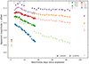 |
Fig. 1. Observed LCs of SN 2024ggi. For clarity, the LCs are shifted by the offsets indicated in the upper legend. Different instruments are indicated with different markers. Rest-frame epochs of optical spectra are marked as grey lines along the top axis. |
LC properties of SN 2024ggi.
The rise times are longer the redder the band is, indicating that the peak is due to a decrease in temperature, corresponding to the well-known cooling phase prior to the recombination of SNe II. The plateau lasts around 90 days in r, i, and z bands, while there is a minor decline in the g band.
3.2. Spectral properties
The spectroscopic data of SN 2024ggi that cover the phases from 5 to 84 days after the explosion are presented in Fig. 2 and compared with the standard Type II plateau SN 1999em. The rest-wavelength positions of the main features are marked with dashed lines. Our spectra cover the interval between 5 and 20 days well, and then there is a gap until 84 days. During the evolution, the continuum becomes less blue with time, consistent with the colour evolution derived from the LCs. As noted by Jacobson-Galán et al. (2024) and Shrestha et al. (2024), in the spectrum at five days after explosion, which is our first spectrum, there is no evidence of high ionisation lines. In the first spectrum, weak, broad absorption features of Hβ, He I λ 4471, and He I λ 5876 are present. The SN evolves slowly during the first 20 days, developing typical P-Cygni profiles. At 13 days, the Hα and Fe II λ 5169 profiles are clearly visible. The velocity of the Hα line, measured from the absorption minimum, goes from ≈ − 9500 to ≈ − 9000 km s−1 between 5 and 20 days, while Fe II λ 5169 velocity varies from ≈–7800 to ≈–6900 km s−1 between 13 and 20 days.
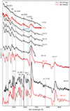 |
Fig. 2. Spectral sequence of SN 2024ggi taken with the JS and Magellan Clay telescopes, marked in black. Main absorption lines are marked with dashed lines at the rest wavelength. Spectra of SN 1999em are shown for comparison in red; epochs are referred to the explosion date derived by Elmhamdi et al. (2003). |
The spectra of SN 2024ggi matches those of typical SNe II, as noticed by the comparison with SN 1999em. However, during the first 20 days of its evolution, the Hα absorption is weaker and less pronounced than that observed in SN 1999em. This weak Hα profile may be associated with the presence of an ejecta–CSM interaction (Hillier & Dessart 2019) and is generally linked to brighter and more rapidly declining SNe II (Gutiérrez et al. 2014). Between 13 and 20 days, the spectra of SN 2024ggi exhibit the ‘Cachito’ feature, an absorption component on the blue side of Hα (Gutiérrez et al. 2017), which is also seen in the 21-day spectrum of SN 1999em. For SN 1999em, this feature had been proposed to be due to high velocity structures in the expanding ejecta of the SN (Baron et al. 2000; Leonard et al. 2002). Since then, it is been identified in different SNe as either high velocity Hα or Si II 6355 Å (Pastorello et al. 2006). If this feature is high-velocity Hα, it would be associated with the interaction between the ejecta and CSM (Chugai et al. 2007). Gutiérrez et al. (2014) proposed that when Cachito is detected within 30 days post-explosion, it is more likely to be associated with Si II, whereas detections at later epochs are linked to high-velocity Hα. Since the Cachito feature in SN2024ggi is observed within this early time frame, it is likely associated with Si II.
At 84 days, the SN has evolved considerably, decreasing its blue continuum and developing features corresponding to Fe II, Sc II, H, and O I. The Hα profile becomes strong, followed by the calcium near-IR triplet feature. This last spectrum covers the wavelength range beyond 7200 Å and until 9700 Å. At this phase, the Hα absorption has shifted to ≈ − 5900 km s−1, and the Fe II λ 5169 to ≈ − 3200 km s−1. All the features described here are marked in Fig. 2. Note that at 84 days, the Cachito feature had disappeared.
3.3. Bolometric evolution
We first calculated the bolometric luminosity of SN 2024ggi. To have accurate constraints on the CSM properties, early observations are needed. Our dataset spans from 5 days to 35 days from explosion in BVRI and from 2 to 106 in griz. Since we only made one observation in the first 5 days after explosion, which are crucial to determine the CSM properties, we added high cadence early photometry of SN 2024ggi published by Shrestha et al. (2024) to our observations. This dataset is composed by ultraviolet (UV) and optical observations in the filters UVW2, UVM2, UVW1, U, B, g, V, r, and i, from the first day until 21 days after explosion.
Although the observations are heavily sampled, magnitude values are sometimes missing for certain filters at a given epoch. To have the LCs with the same cadence across all filters, we linearly interpolated them. The gap between consecutive epochs to interpolate was always less than 2.5 days.
The next step is to correct the observed magnitudes by extinction. Regarding the Milky Way (MW) extinction, the recalibrated dust maps of Schlegel et al. (1998) yield a value of E(B − V)MW = 0.07 mag (Schlafly & Finkbeiner 2011) from the NASA Extragalactic Database (NED1), considering an extinction law from Cardelli et al. (1989) with RV = 3.1. Pessi et al. (2024) find three intervening galactic clouds in the line of sight to the SN using high-resolution spectroscopy, inferring a total extinction of E(B − V)MW = 0.12 ± 0.02 mag. This value does not compare well with the extinction from the recalibrated maps of Schlafly & Finkbeiner (2011). As noted by Pessi et al. (2024), the dust extinction map of Schlegel et al. (1998) is less accurate when multiple dust clouds with different temperatures are encountered, which may explain the discrepancy. Additionally, several estimates have been made for the host galaxy component of the extinction for this SN. Jacobson-Galán et al. (2024) inferred an E(B − V)host = 0.084 ± 0.018 mag by calculating the Na I D1 and D2 equivalent widths from high resolution spectra, and using the calibrations from Stritzinger et al. (2018). Similarly, Pessi et al. (2024) calculated the host extinction to be E(B − V)host = 0.036 ± 0.007 mag, and Shrestha et al. (2024) measured E(B − V)host = 0.034 ± 0.020 mag, both using the calibrations from Poznanski et al. (2012). In summary, Jacobson-Galán et al. (2024), Pessi et al. (2024), and Shrestha et al. (2024) calculate a total E(B − V)tot of 0.154, 0.16, and 0.154 mag respectively. We assumed E(B − V)tot = 0.16 mag.
After correcting the interpolated LCs by extinction, we converted them to monochromatic fluxes at the effective wavelength of each band. Then, we integrated the monochromatic fluxes along wavelength for each epoch, obtaining the quasi-bolometric flux (Fqbol). To account for the flux outside the observed wavelength range, we assumed that at early epochs, the SN emission is well represented by a blackbody (BB) distribution. We then extrapolated the UV and IR to obtain the unobserved UV and IR flux (FUV and FIR, respectively), by fitting a BB to the spectral energy distributions at each epoch. Blackbody fits were restricted to observational epochs with at least four bands, whether observed or interpolated. Then, the total bolometric flux was calculated as Fbol = FUV + Fqbol + FIR, and converted to luminosity assuming the distance stated in the introduction. The uncertainty in the luminosity was estimated by considering uncertainties in the photometry, distance, and the estimated errors of the extrapolated fluxes.
Our high-cadence data extend up to ∼85 days post-explosion, then there is a 12 day gap before our last observation at 106 days post-explosion. Since this gap is too long to extrapolate, to calculate the bolometric LC beyond 85 days we used public photometry available in the B and V bands from the American Association of Variable Star Observers (AAVSO) web page2 (Kloppenborg 2024). Around ∼250 photometric measurements in the B band and ∼400 in the V band are available contributed by different observers globally for SN 2024ggi, covering 125 days of the SN evolution. We adopted the mean magnitudes in daily bins after rejecting discrepant observations, beginning from 85 days post-explosion where our original data concluded. We corrected the magnitudes by extinction, and then we used the (B-V) colour-based bolometric corrections from Martinez et al. (2022a) to derive the bolometric magnitudes. The bolometric luminosities were then calculated using the distance adopted in the introduction. The uncertainties were calculated considering uncertainties in the photometry and in the bolometric corrections.
The complete bolometric LC is shown in Fig. 3. We determined the bolometric magnitude at maximum to be Mmax = −18.920 ± 0.001 mag, and calculated the morphological bolometric LC parameters as defined by Martinez et al. (2022a, see their Fig. 8 and Anderson et al. 2014). These parameters essentially characterise the bolometric magnitudes in different parts of the LC, decline rates, and duration of the different phases. In summary each parameter is defined as follows: s1, s2, and s3 are the decline rates in magnitudes per 100 days during the cooling phase, the plateau phase, and the radioactive tail phase, respectively. The parameter ttrans corresponds to the epoch of transition between the cooling decline and the plateau decline. optd, pd, and Cd correspond to the duration of the optically thick, plateau, and cooling phases, respectively. Finally, Mbol, end and Mbol, tail are the bolometric magnitudes measured 30 days before and after tPT, respectively, where tPT is equivalent to optd. Due to the lack of data during the radioactive tail phase at the time of these calculations, we did not include values for Mtail or the s3 decline rate. The results are listed on Table 3, together with the comparison of the same parameters for SN 2023ixf from Bersten et al. (2024). Additionally, we include in Table 3 the parameters calculated by Martinez et al. (2022a) using a large sample of SNe II from the Carnegie Supernova Project-I (CSP-I; Hamuy et al. 2006).
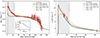 |
Fig. 3. Observations of SN 2024ggi (points) compared with hydrodynamical models (lines). Left panel: Bolometric LC. The inset shows density profiles of the models with no CSM (black), with a steady wind (yellow), and with an accelerated wind (blue). Right panel: Photospheric velocity evolution. The shaded grey area marks the approximate time frame during which the emission is dominated mainly by CSM interaction, i.e. times t ≲ Cd = 26 d. The uncertainty on the velocities is taken as ≈ − 500 km s−1, and this takes the resolution of the spectra and the error in the measurements into account. |
Bolometric LC parameters of SN 2024ggi.
We find that most parameters of SN 2024ggi, similar to SN 2023ixf, fall within 1σ of the comparison distributions, suggesting it is a typical SN II. However, we note some minor deviations: SN 2024ggi exhibits a longer plateau duration and declines faster in the cooling phase than average, contrary to which was obtained for SN 2023ixf, which exhibited a shorter plateau duration, compared to the distribution of SNe II. A longer plateau duration suggests a more massive progenitor than the bulk of SNe II (Martinez et al. 2022b, see also our Sect. 4).
4. Hydrodynamical modelling
We aimed to infer the progenitor and CSM properties by comparing the bolometric LC and velocity evolution to models computed using the one-dimensional Lagrangian local thermodynamic equilibrium radiation hydrodynamics code from Bersten et al. (2011). Given that moderate CSM structures do not significantly influence bolometric LCs of SNe II at times ≳ 30 d (Morozova et al. 2018; Martinez et al. 2022b), it is practical to divide the SN 2024ggi modelling into two steps.
In Sect. 4.1 we focus on inferring the global parameters such as the explosion energy (Eexp), the progenitor mass and radius, and the nickel mass (M56Ni) and its mixing (mix(56Ni)3) by matching the plateau luminosity and duration, as well as the Fe II line velocities with our models. In Sect. 4.2 we then focus on deriving the CSM parameters such as the CSM extension (RCSM) and mass-loss rate (Ṁ) for different wind prescriptions (steady and accelerated). The CSM was artificially included in the outermost regions of our progenitor models. We then matched the cooling phase luminosity, duration, and steepness, as well as the line velocities, with our models. In this work, we adopted a cooling phase duration of Cd = 26 d, derived from the bolometric LC (see Sect. 3.3), to distinguish the CSM interaction-dominated phase from the rest of the evolution. Lastly, a complete model was calculated using the parameter set derived from the two-step modelling.
4.1. Global parameter modelling
Our hydrodynamical code requires progenitor models at the time of core collapse in order to initialise the explosion. For this work we utilised a pre-SN model grid calculated by Nomoto & Hashimoto (1988), which comprises a RSG set with ZAMS masses of 13, 15, 18, 20, and 25 M⊙. For simplicity, we refer to these progenitor models by their ZAMS masses prefixed with the letter M (e.g. M13). The main properties of our pre-SN models are listed in Table 4. The explosion is then simulated by depositing some energy in the form of a thermal bomb at a mass coordinate where the pre-SN structure is assumed to collapse into a compact remnant (Mcore), and is thus removed from our calculations.
Properties of the pre-SN model grid calculated by Nomoto & Hashimoto (1988) used in this work.
A set of hydrodynamical models was generated by varying several physical parameters for each of our pre-SN models. We explored different values of Eexp in the range 0.5 − 1.7 foe (1 foe = 1051 erg), M56Ni in the range 0.01 − 0.06 M⊙ and mix(56Ni) in the range 10 − 80%. Then, we visually compared the model set with the bolometric LC and Fe II line velocities of SN 2024ggi derived in Sects. 3.2 and 3.3 to select our preferred model.
To choose an adequate progenitor model, we used the well-known fact that for a given pre-SN model (with a fixed mass and radius), Eexp is the only parameter that can modify the ejecta expansion velocities (Kasen & Woosley 2009; Dessart et al. 2013; Bersten 2013). Thus, our initial exploration focused on finding appropriate Eexp values to reproduce the Fe II velocities of SN 2024ggi across our pre-SN model grid. From this analysis, we find that only the M13, M15, and M18 models could reproduce the Fe II line velocities using Eexp values of 1.5, 1.2, and 1.7 foe, respectively, and also provide a reasonable LC of SN 2024ggi. For more massive models, no solution was found.
Subsequently, we focused on refining the bolometric LC match through an exploration of the nickel mass and distribution (M56Ni and mix(56Ni)), the remaining free parameters available. From this exploration we find that M15 models provide an overall better agreement with the observations of SN 2024ggi.
In Fig. 3 we present our preferred solution, which corresponds to the M15 model with an explosion energy of Eexp = 1.2 foe and a 56Ni mass of M56Ni = 0.035 M⊙ with mix(56Ni) = 30%. We also present two additional models, M13 (dashed green line) and M18 (dashed pink line), as a comparison. Although these models provide a comparable match to the Fe II velocities as our preferred M15 model, the same is not true for the LC of SN 2024ggi. As can be seen in Fig. 3, both models have a steeper plateau decline rate than what is observed, overestimate the plateau luminosity early on, and produce a shorter (M13) or longer (M18) plateau duration. Therefore, these models produce a poorer match to the data than our preferred M15 model. However, we cannot rule out some intermediate models from our analysis.
The M15 model provides a good representation of the plateau, the transition, and the onset of the radioactive tail. However, we posit that the derived nickel properties should be taken with caution due to the relatively large uncertainties starting at t ∼ 87 d, combined with the lack of observations beyond t ∼ 124 d after the explosion. Nevertheless, given the strong correlation between radioactive tail luminosity and 56Ni mass (Martinez et al. 2022c), it is possible to rule out values of M56Ni ≳ 0.035 M⊙, as they produce radioactive tail luminosities exceeding the faintest observed transition luminosity. We also note that our choice of progenitor and Eexp parameters is not altered by the exploration of nickel parameters, as these do not affect the expansion velocities and have a comparatively small influence on the plateau characteristics.
From our exploration, we conclude that the M15 model with an explosion energy of Eexp = 1.2 foe, a 56Ni mass of M56Ni = 0.035 M⊙ with mix(56Ni) = 30% is a model that closely represents the Fe II velocities and the bolometric LC of SN 2024ggi at times t ≳ 26 d. This model is presented in Fig. 3. Although our analysis is based on visual comparisons, we deem our choice of the optimal physical parameters to be well justified within the assumptions of our modelling. A more refined statistical analysis is beyond the scope of this study.
4.2. CSM parameter modelling
The models presented in Sect. 4.1 fail to reproduce the early observations since they underestimate the bolometric luminosity up to t ∼ 26 d. This discrepancy has been attributed to the effect of the interaction between the ejecta and an existing CSM. It has been established that the incorporation of a CSM distribution at the outermost layers of the pre-SN structure increases the luminosity of the resulting model during the cooling phase, thus improving the early-time modelling (Moriya et al. 2011; Morozova et al. 2018; Englert Urrutia et al. 2020). The presence of CSM also lowers the maximum photospheric velocity and halts the velocity decline during the cooling phase, which can help constrain the plausible CSM configurations. The existence of a CSM structure in SN 2024ggi is further supported by the presence of flash features in the early-time spectra (Hoogendam et al. 2024; Jacobson-Galán et al. 2024; Pessi et al. 2024; Chen et al. 2024; Shrestha et al. 2024).
On that basis, we modified the density profile of the M15 progenitor model by attaching a CSM distribution before simulating the explosion. We used the same explosion parameters as those of our preferred model presented in Sect. 4.1. Only the CSM properties are explored, which mainly affect the LC and expansion velocities for t ≲ 26 d. We note that different CSM configurations introduce slight variations during the transition to the radioactive tail. However, these differences are too small to warrant a re-evaluation of the model parameters derived in Sect. 4.1.
In this section we present two different scenarios: a steady wind distribution (ρ ∝ r−2) and an accelerated wind distribution. In both cases, a set of models was explored and visually compared with the SN 2024ggi data. In the following, we present and discuss the best models found within our exploration. However, it must be noted that we cannot rule out other possible solutions given the qualitative nature of our analysis and the well-known degeneracies between CSM parameters (Dessart & Jacobson-Galán 2023; Khatami & Kasen 2024). To refine the parameter exploration, a statistical study with a broader parameter grid needs to be performed, which is left for future work.
For the steady wind scenario, the wind velocity was fixed at vw = 77 km s−1, as measured by Pessi et al. (2024), and different CSM extensions and mass-loss rates were explored. Note that Shrestha et al. (2024) measured a vw = 37 km s−1 from the full width at half maximum (FWHM) of the Hα line. However, the FWHM corresponds to vw only in the optically thin case, which might not be the case for 2024ggi at the epoch when those measurements were made. We used the measurements from the narrow component of Hα assuming that an optically thick CSM is a better proxy for vw.
The preferred steady-wind model is shown in Fig. 3, and it greatly improves the early LC and expansion velocities modelling as a result of the inclusion of this CSM. Said model has an extension of RCSM = 1200 R⊙ and a mass-loss rate of Ṁ = 3.6 M⊙ yr−1, corresponding to a CSM mass of MCSM = 0.7 M⊙. The inferred mass-loss rate is considerably higher than the typical range for SNe II-P, suggesting an enhanced mass loss event during the last ∼ 70 d before the explosion (Morozova et al. 2017).
We also examined whether this model was able to reproduce the duration of the flash features in the observed spectra. Following Dessart et al. (2017), the narrow lines last as long as the shock is placed within a slow-moving optically thick material (i.e. until the shock goes through the SN photosphere). In our model we find that the flash features should disappear ∼0.1 d after shock breakout. This duration is an order of magnitude lower than the estimated value of 3.8 ± 1.6 d for SN 2024ggi (Jacobson-Galán et al. 2024) and could be a plausible reason to consider the steady wind model less favourably.
For the accelerated wind scenario, we followed the wind velocity prescription given by Moriya et al. (2018), which takes the form of the β velocity law given below:
 (1)
(1)
where v0 is the initial wind velocity (0.1 km s−1), v∞ is the terminal wind velocity (77 km s−1, Pessi et al. 2024), R0 is the radial coordinate where the CSM is attached to the progenitor model, and β is the wind acceleration parameter (Lamers & Cassinelli 1999).
We then explored different CSM extensions, mass-loss rates and wind acceleration parameters, and compared the resulting model grid with the early-time bolometric LC and line velocities. The preferred accelerated wind model has an extension of RCSM = 3000 R⊙, a mass-loss rate of Ṁ = 4.6 × 10⁻³ M⊙ yr−1 and a wind acceleration parameter of β = 9, corresponding to a CSM mass of MCSM = 0.55 M⊙. This model, shown in Fig. 3, greatly improves the modelling of early-time observations compared to the CSM-free model. It produces a bolometric LC similar to the steady wind model, albeit more luminous and with a steeper decline rate during the first ∼ 15 d of evolution. Likewise, the photospheric velocity evolutions of the two CSM models are comparable, although the accelerated wind model yields slightly lower velocities during the first ∼ 15 d. Since Fe II velocity measurements before t ≲ 15 d are lacking, we cannot further constrain the CSM properties of SN 2024ggi. Nevertheless, the maximum ejecta velocity during the first ∼ 15 d of all our models never exceeds 9000 km s−1, which is in agreement with the results by Hu et al. (2025), where the shock velocity is reported to be approximately 10 000 km s−1.
We note that the optimal wind acceleration parameter found in our exploration is higher than the typical range for normal RSGs (1–5, Moriya et al. 2018). This would be consistent with an enhanced mass-loss event scenario prior to the explosion. We also examined the duration of the flash features, and found that they should last for ∼2.4 d after shock breakout. This is an improvement over the relatively short-lived prediction in our preferred steady wind model, and closer to, though still shorter than the estimated duration in SN 2024ggi (3.8 ± 1.6 d, Jacobson-Galán et al. 2024).
Despite the accelerated wind scenario producing a Ṁ value three orders of magnitude lower than the steady wind model, the total MCSM remains roughly similar in the two cases. This consistency in the inferred MCSM is noteworthy, as it suggests that a similar amount of material was needed in both scenarios to decelerate the shock wave and thereby produce lower expansion velocities. On the other hand, the mass-loss rate is associated with the late evolutionary history of the progenitor star, and thus remains largely unconstrained despite recent efforts (Quataert & Shiode 2012; Woosley & Heger 2015; Fuller & Tsuna 2024).
The density profiles of the steady and accelerated wind models are shown in the inset of Fig. 3. The two CSM profiles exhibit similar density and steepness up to a radius of R ≃ 1000 R⊙, indicating the presence of a dense and compact CSM core. Beyond this extension, in the range of R ≃ 1000 − 3000 R⊙, the accelerated wind model shows a sharp drop in density forming a low-density tail. This configuration – an inner dense and compact core coupled with an outer light and extended tail – resembles the two-component CSM distribution proposed in recent studies (Chugai & Utrobin 2022; Jacobson-Galán et al. 2023; Hu et al. 2025; Zimmerman et al. 2024). The two-component CSM models offer a promising pathway to explain the CSM mass required to reproduce the early-time bolometric LC while providing more realistic mass-loss scenarios. Therefore, we consider the accelerated wind model to be the more reasonable prescription for the CSM structure of SN 2024ggi, which in turn provides a more credible timescale for the duration of the flash features as discussed above.
5. Conclusions
In this work we present optical photometric and spectroscopic observations of the Type II SN 2024ggi, spanning from 2 to 106 days after the explosion. Similar to SN 2023ixf, SN 2024ggi is among the closest SNe of the decade, providing a unique opportunity to constrain the progenitor properties of SNe II. The analysis of the bolometric LC suggests that SN 2024ggi is a typical Type II SN. Nevertheless, it shows a longer plateau duration and a faster decline in the cooling phase compared to a distribution of SNe II. We have presented the first hydrodynamical modelling of the bolometric LC and photospheric velocity evolution of SN 2024ggi, using the full extent of the plateau phase. Our results suggest that SN 2024ggi originated from the explosion of a star with a ZAMS mass of 15 M⊙, an explosion energy of 1.2 × 1051 erg, a 56Ni production of ≲0.035 M⊙, and a relatively moderate 56Ni mixing of 30%. The exploded RSG star at the final stage of its evolution had a mass of 14 M⊙ and a radius of 516 R⊙.
To characterise the CSM around the progenitor star, we modelled the early phases of the explosion by modifying the outermost density profile and considering two different scenarios: steady winds and accelerated winds. In the steady wind case, the preferred model suggests a CSM extension of 1200 R⊙ (8.3 × 1013 cm) with a mass-loss rate of 3.6 M⊙ yr−1, corresponding to a total CSM mass of 0.7 M⊙. This model predicts a maximum flash features duration of 0.1 d. For the accelerated wind case, the preferred model points to a CSM extension of 3000 R⊙ (2.1 × 1014 cm) with a mass-loss rate of 4 × 10⁻³ M⊙ yr−1 and an acceleration parameter of β = 9, resulting in a similar CSM mass of 0.55 M⊙. In this case, the duration of the flash features is 2.4 d, which is closer to the observations. While both models reproduce the bolometric LC and expansion velocity evolution reasonably well, we consider the accelerated wind scenario to be more reasonable as it provides a lower mass-loss rate and a slightly better agreement with the duration of the flash features.
Several works in the literature have analysed the early properties of SN 2024ggi, which gave us something to compare our inferred parameters with. Studies modelling early spectra of SN 2024ggi found a CSM confined to a range of RCSM = 2.7 − 5 × 1014 cm (3900–7200 R⊙), formed from a progenitor with a mass-loss rate in the range 10−3 − 10−2 M⊙ yr−1 (Jacobson-Galán et al. 2024; Shrestha et al. 2024; Zhang et al. 2024b). Additionally, Chen et al. (2025) present a hydrodynamical model of the first ∼ 15 days of only the LC information and find that the data are well matched by a model with an explosion energy of 2 × 1051 erg, a mass-loss rate of 10−3 M⊙ yr−1 (assuming an accelerated wind with β = 4.0 and a terminal wind velocity of 10 km s−1), and a confined CSM with a radius of RCSM = 6 × 1014 cm (∼8600 R⊙) and a mass of 0.4 M⊙. Despite the difference in methodology, our estimations of the CSM parameters, except for RCSM, are in agreement with those calculated in the literature.
Studies analysing the pre-explosion data of the SN site identified a RSG star with an estimated mass ranging from 13 to 17 M⊙ as a progenitor candidate of SN 2024ggi (Xiang et al. 2024; Chen et al. 2025). Furthermore, environmental studies of the SN site suggest a lower-mass progenitor, compatible with 10 M⊙ (Hong et al. 2024). Our findings align with the estimates derived from direct detections. Moreover, our analysis of the morphological parameters of the bolometric LC of SN 2024ggi reveals a longer plateau compared to SN 2023ixf and a sample of SNe II from the CSP-I. This suggests that the progenitor of SN2024ggi was more massive than that of SN2023ixf and the average progenitor mass in the CSP-I sample, in line with what we find in our hydrodynamic modelling.
The recent detection of two of the closest SNe II of the decade, SN 2023ixf and SN 2024ggi, highlights the importance of early, high-cadence observations in constraining the physics of both the explosion and the progenitor stars of SNe II. Continued monitoring of SN 2024ggi during the nebular phase and after its emission fades, to confirm the disappearance of the progenitor candidate, will provide critical insights into its nature.
Data availability
The spectra presented in this paper are available via the WISeREP4 archive (Yaron & Gal-Yam 2012).
The 56Ni mixing is defined as the percentage of the total pre-SN mass to which the 56Ni is uniformly distributed.
Acknowledgments
This work is based on data acquired at Complejo Astronómico El Leoncito, operated under agreement between the Consejo Nacional de Investigaciones Científicas y Técnicas de la República Argentina and the National Universities of La Plata, Córdoba and San Juan. We thank the authorities of CASLEO, for the prompt response that made possible to obtain the data. This paper includes data gathered with the 6.5 meter Magellan Telescopes located at Las Campanas Observatory, Chile, and observations from the Las Cumbres Observatory global telescope network under the program allocated by the Chilean Telescope Allocation Committee (CNTAC), no: CN2024B-35. E.H. was supported from ANID, Beca Doctorado Folio #21222163. R.C. acknowledges support from Gemini ANID ASTRO21-0036. M.O. acknowledges support from UNRN PI2022 40B1039 grant. M.G. acknowledges support from ANID, Millennium Science Initiative, AIM23-0001. J.L.P acknowledges support from ANID, Millennium Science Initiative, AIM23-0001.
References
- Anderson, J. P., González-Gaitán, S., Hamuy, M., et al. 2014, ApJ, 786, 67 [Google Scholar]
- Baron, E., Branch, D., Hauschildt, P. H., et al. 2000, ApJ, 545, 444 [Google Scholar]
- Bersten, M. C. 2013, arXiv e-prints [arXiv:1303.0639] [Google Scholar]
- Bersten, M. C., Benvenuto, O., & Hamuy, M. 2011, ApJ, 729, 61 [NASA ADS] [CrossRef] [Google Scholar]
- Bersten, M. C., Orellana, M., Folatelli, G., et al. 2024, A&A, 681, L18 [NASA ADS] [CrossRef] [EDP Sciences] [Google Scholar]
- Brennan, S. J., & Fraser, M. 2022, A&A, 667, A62 [NASA ADS] [CrossRef] [EDP Sciences] [Google Scholar]
- Bruch, R. J., Gal-Yam, A., Yaron, O., et al. 2023, ApJ, 952, 119 [NASA ADS] [CrossRef] [Google Scholar]
- Cardelli, J. A., Clayton, G. C., & Mathis, J. S. 1989, ApJ, 345, 245 [Google Scholar]
- Cartier, R., Contreras, C., Stritzinger, M., et al. 2024, A&A, submitted, [arXiv:2410.21381] [Google Scholar]
- Chandra, P., Maeda, K., Nayana, A. J., et al. 2024, ATel, 16612, 1 [Google Scholar]
- Chen, X., Kumar, B., Er, X., et al. 2024, ApJ, 971, L2 [Google Scholar]
- Chen, T.-W., Yang, S., Srivastav, S., et al. 2025, ApJ, 983, 86 [Google Scholar]
- Chugai, N., & Utrobin, V. 2022, Astron. Lett., accepted [arXiv:2205.07749] [Google Scholar]
- Chugai, N. N., Chevalier, R. A., & Utrobin, V. P. 2007, ApJ, 662, 1136 [NASA ADS] [CrossRef] [Google Scholar]
- Contreras, C., Hamuy, M., Phillips, M. M., et al. 2010, AJ, 139, 519 [Google Scholar]
- Dessart, L., & Jacobson-Galán, W. V. 2023, A&A, 677, A105 [NASA ADS] [CrossRef] [EDP Sciences] [Google Scholar]
- Dessart, L., Hillier, D. J., Waldman, R., & Livne, E. 2013, MNRAS, 433, 1745 [NASA ADS] [CrossRef] [Google Scholar]
- Dessart, L., Hillier, D. J., Audit, E., Livne, E., & Waldman, R. 2016, MNRAS, 458, 2094 [Google Scholar]
- Dessart, L., Hillier, D. J., & Audit, E. 2017, A&A, 605, A83 [NASA ADS] [CrossRef] [EDP Sciences] [Google Scholar]
- Elmhamdi, A., Danziger, I. J., Chugai, N., et al. 2003, MNRAS, 338, 939 [CrossRef] [Google Scholar]
- Englert Urrutia, B. N., Bersten, M. C., & Cidale, L. S. 2020, Boletin de la Asociacion Argentina de Astronomia La Plata Argentina, 61B, 51 [Google Scholar]
- Marti-Devesa, G., & Fermi-LAT Collaboration. 2024, ATel, 16601, 1 [Google Scholar]
- Ferrari, L., Folatelli, G., Ertini, K., Kuncarayakti, H., & Andrews, J. E. 2024, A&A, 687, L20 [NASA ADS] [CrossRef] [EDP Sciences] [Google Scholar]
- Flewelling, H. A., Magnier, E. A., Chambers, K. C., et al. 2020, ApJS, 251, 7 [NASA ADS] [CrossRef] [Google Scholar]
- Fuller, J., & Tsuna, D. 2024, Open J. Astrophys., 7, 47 [CrossRef] [Google Scholar]
- Gutiérrez, C. P., Anderson, J. P., Hamuy, M., et al. 2014, ApJ, 786, L15 [CrossRef] [Google Scholar]
- Gutiérrez, C. P., Anderson, J. P., Hamuy, M., et al. 2017, ApJ, 850, 89 [CrossRef] [Google Scholar]
- Hamuy, M., Folatelli, G., Morrell, N. I., et al. 2006, PASP, 118, 2 [NASA ADS] [CrossRef] [Google Scholar]
- Hillier, D. J., & Dessart, L. 2019, A&A, 631, A8 [NASA ADS] [CrossRef] [EDP Sciences] [Google Scholar]
- Hong, X., Sun, N.-C., Niu, Z., et al. 2024, ApJ, 977, L50 [Google Scholar]
- Hoogendam, W., Auchettl, K., Tucker, M., et al. 2024, TNSAN, 103, 1 [Google Scholar]
- Hu, M., Ao, Y., Yang, Y., et al. 2025, ApJ, 978, L27 [Google Scholar]
- Itagaki, K. 2023, TNSTR, 2023-1158, 1 [Google Scholar]
- Jacobson-Galán, W. V., Dessart, L., Margutti, R., et al. 2023, ApJ, 954, L42 [CrossRef] [Google Scholar]
- Jacobson-Galán, W. V., Davis, K. W., Kilpatrick, C. D., et al. 2024, ApJ, 972, 177 [CrossRef] [Google Scholar]
- Jencson, J. E., Pearson, J., Beasor, E. R., et al. 2023, ApJ, 952, L30 [NASA ADS] [CrossRef] [Google Scholar]
- Kasen, D., & Woosley, S. E. 2009, ApJ, 703, 2205 [NASA ADS] [CrossRef] [Google Scholar]
- Khatami, D. K., & Kasen, D. N. 2024, ApJ, 972, 140 [NASA ADS] [CrossRef] [Google Scholar]
- Killestein, T., Ackley, K., Kotak, R., et al. 2024, TNSAN, 101, 1 [Google Scholar]
- Kilpatrick, C. D., Foley, R. J., Jacobson-Galán, W. V., et al. 2023, ApJ, 952, L23 [NASA ADS] [CrossRef] [Google Scholar]
- Kloppenborg, B. K. 2024, Observations from the AAVSO International Database, https://www.aavso.org, accessed: 2024-10-01 [Google Scholar]
- Komura, Y., Matsunaga, K., Uchida, H., & Enoto, T. 2024, ATel, 16595, 1 [Google Scholar]
- Koribalski, B. S., Staveley-Smith, L., Kilborn, V. A., et al. 2004, AJ, 128, 16 [Google Scholar]
- Lamers, H. J. G. L. M., & Cassinelli, J. P. 1999, Introduction to Stellar Winds (Cambridge, UK: Cambridge University Press) [Google Scholar]
- Leonard, D. C., Filippenko, A. V., Gates, E. L., et al. 2002, PASP, 114, 35 [Google Scholar]
- Liu, C., Chen, X., Er, X., et al. 2023, ApJ, 958, L37 [NASA ADS] [CrossRef] [Google Scholar]
- Lutovinov, A. A., Semena, A. N., Mereminskiy, I. A., et al. 2024, ATel, 16586, 1 [Google Scholar]
- Margutti, R., & Grefenstette, B. 2024, ATel, 16587, 1 [Google Scholar]
- Martinez, L., Bersten, M. C., Anderson, J. P., et al. 2022a, A&A, 660, A40 [NASA ADS] [CrossRef] [EDP Sciences] [Google Scholar]
- Martinez, L., Bersten, M. C., Anderson, J. P., et al. 2022b, A&A, 660, A41 [NASA ADS] [CrossRef] [EDP Sciences] [Google Scholar]
- Martinez, L., Anderson, J. P., Bersten, M. C., et al. 2022c, A&A, 660, A42 [NASA ADS] [CrossRef] [EDP Sciences] [Google Scholar]
- Moriya, T., Tominaga, N., Blinnikov, S. I., Baklanov, P. V., & Sorokina, E. I. 2011, MNRAS, 415, 199 [NASA ADS] [CrossRef] [Google Scholar]
- Moriya, T. J., Förster, F., Yoon, S.-C., Gräfener, G., & Blinnikov, S. I. 2018, MNRAS, 476, 2840 [Google Scholar]
- Morozova, V., Piro, A. L., & Valenti, S. 2017, ApJ, 838, 28 [NASA ADS] [CrossRef] [Google Scholar]
- Morozova, V., Piro, A. L., & Valenti, S. 2018, ApJ, 858, 15 [Google Scholar]
- Neustadt, J. M. M., Kochanek, C. S., & Smith, M. R. 2024, MNRAS, 527, 5366 [Google Scholar]
- Niu, Z., Sun, N.-C., Maund, J. R., et al. 2023, ApJ, 955, L15 [NASA ADS] [CrossRef] [Google Scholar]
- Nomoto, K., & Hashimoto, M. 1988, Phys. Rep., 163, 13 [CrossRef] [Google Scholar]
- Pastorello, A., Sauer, D., Taubenberger, S., et al. 2006, MNRAS, 370, 1752 [NASA ADS] [CrossRef] [Google Scholar]
- Paturel, G., Teerikorpi, P., Theureau, G., et al. 2002, A&A, 389, 19 [NASA ADS] [CrossRef] [EDP Sciences] [Google Scholar]
- Pérez-Fournon, I., Poidevin, F., Aguado, D. S., et al. 2024, TNSAN, 107, 1 [Google Scholar]
- Perley, D. A., Gal-Yam, A., Irani, I., & Zimmerman, E. 2023, TNSAN, 119, 1 [NASA ADS] [Google Scholar]
- Pessi, T., Cartier, R., Hueichapan, E., et al. 2024, A&A, 688, L28 [NASA ADS] [CrossRef] [EDP Sciences] [Google Scholar]
- Poznanski, D., Prochaska, J. X., & Bloom, J. S. 2012, MNRAS, 426, 1465 [Google Scholar]
- Qin, Y.-J., Zhang, K., Bloom, J., et al. 2024, MNRAS, 534, 271 [NASA ADS] [CrossRef] [Google Scholar]
- Quataert, E., & Shiode, J. 2012, MNRAS, 423, L92 [NASA ADS] [CrossRef] [Google Scholar]
- Ryder, S., Maeda, K., Chandra, P., Alsaberi, R., & Kotak, R. 2024, ATel, 16616, 1 [Google Scholar]
- Schlafly, E. F., & Finkbeiner, D. P. 2011, ApJ, 737, 103 [Google Scholar]
- Schlegel, E. M. 1990, MNRAS, 244, 269 [NASA ADS] [Google Scholar]
- Schlegel, D. J., Finkbeiner, D. P., & Davis, M. 1998, ApJ, 500, 525 [Google Scholar]
- Shrestha, M., Bostroem, K. A., Sand, D. J., et al. 2024, ApJ, 972, L15 [Google Scholar]
- Soraisam, M. D., Szalai, T., Van Dyk, S. D., et al. 2023, ApJ, 957, 64 [NASA ADS] [CrossRef] [Google Scholar]
- Srivastav, S., Chen, T. W., Smartt, S. J., et al. 2024, TNSAN, 100, 1 [Google Scholar]
- Stritzinger, M. D., Taddia, F., Burns, C. R., et al. 2018, A&A, 609, A135 [NASA ADS] [CrossRef] [EDP Sciences] [Google Scholar]
- Tody, D. 1986, in Instrumentation in astronomy VI, ed. D. L. Crawford, Society of Photo-Optical Instrumentation Engineers (SPIE) Conference Series, 627, 733 [Google Scholar]
- Tonry, J. L., Denneau, L., Heinze, A. N., et al. 2018, PASP, 130, 064505 [Google Scholar]
- Van Dyk, S. D., Srinivasan, S., Andrews, J. E., et al. 2024, ApJ, 968, 27 [NASA ADS] [CrossRef] [Google Scholar]
- Woosley, S. E., & Heger, A. 2015, ApJ, 810, 34 [NASA ADS] [CrossRef] [Google Scholar]
- Xiang, D., Mo, J., Wang, X., et al. 2024, ApJ, 969, L15 [Google Scholar]
- Yang, S., Chen, T. W., Stevance, H. F., et al. 2024, TNSAN, 105, 1 [Google Scholar]
- Yaron, O., & Gal-Yam, A. 2012, PASP, 124, 668 [Google Scholar]
- Yaron, O., Perley, D. A., Gal-Yam, A., et al. 2017, Nat. Phys., 13, 510 [NASA ADS] [CrossRef] [Google Scholar]
- Zhai, Q., Li, L., Zhang, J., & Wang, X. 2024, TNS Classif. Rep., 2024-1031, 1 [Google Scholar]
- Zhang, J., Li, C. K., Cheng, H. Q., et al. 2024a, ATel, 16588, 1 [Google Scholar]
- Zhang, J., Dessart, L., Wang, X., et al. 2024b, ApJ, 970, L18 [NASA ADS] [CrossRef] [Google Scholar]
- Zimmerman, E. A., Irani, I., Chen, P., et al. 2024, Nature, 627, 759 [Google Scholar]
Appendix A: Tables
Optical photometry of SN 2024ggi from the HSH and JS telescopes.
Optical photometry of SN 2024ggi from the LCOGTN 1m telescope.
All Tables
Properties of the pre-SN model grid calculated by Nomoto & Hashimoto (1988) used in this work.
All Figures
|
Fig. 1. Observed LCs of SN 2024ggi. For clarity, the LCs are shifted by the offsets indicated in the upper legend. Different instruments are indicated with different markers. Rest-frame epochs of optical spectra are marked as grey lines along the top axis. |
| In the text | |
|
Fig. 2. Spectral sequence of SN 2024ggi taken with the JS and Magellan Clay telescopes, marked in black. Main absorption lines are marked with dashed lines at the rest wavelength. Spectra of SN 1999em are shown for comparison in red; epochs are referred to the explosion date derived by Elmhamdi et al. (2003). |
| In the text | |
|
Fig. 3. Observations of SN 2024ggi (points) compared with hydrodynamical models (lines). Left panel: Bolometric LC. The inset shows density profiles of the models with no CSM (black), with a steady wind (yellow), and with an accelerated wind (blue). Right panel: Photospheric velocity evolution. The shaded grey area marks the approximate time frame during which the emission is dominated mainly by CSM interaction, i.e. times t ≲ Cd = 26 d. The uncertainty on the velocities is taken as ≈ − 500 km s−1, and this takes the resolution of the spectra and the error in the measurements into account. |
| In the text | |
Current usage metrics show cumulative count of Article Views (full-text article views including HTML views, PDF and ePub downloads, according to the available data) and Abstracts Views on Vision4Press platform.
Data correspond to usage on the plateform after 2015. The current usage metrics is available 48-96 hours after online publication and is updated daily on week days.
Initial download of the metrics may take a while.