SN 2023ixf: An average-energy explosion with circumstellar medium and a precursor

Alexandra Kozyreva; Andrea Caputo; Petr Baklanov; Alexey Mironov; Hans-Thomas Janka

doi:10.1051/0004-6361/202452758

Home

All issues

Volume 694 (February 2025)

A&A, 694 (2025) A319

Full HTML

Open Access

Issue		A&A Volume 694, February 2025


Article Number		A319
Number of page(s)		18
Section		Stellar structure and evolution
DOI		https://doi.org/10.1051/0004-6361/202452758
Published online		24 February 2025

A&A, 694, A319 (2025)

SN 2023ixf: An average-energy explosion with circumstellar medium and a precursor

Alexandra Kozyreva¹^⋆, Andrea Caputo²^,3, Petr Baklanov⁴^,5^,6, Alexey Mironov⁶ and Hans-Thomas Janka⁷

¹ Heidelberger Institut für Theoretische Studien, Schloss-Wolfsbrunnenweg 35, D-69118 Heidelberg, Germany
² Theoretical Physics Department, CERN, 1211 Geneva 23, Switzerland
³ Dipartimento di Fisica, “Sapienza” Università di Roma & Sezione INFN Roma1, Piazzale Aldo Moro 5, 00185 Roma, Italy
⁴ National Research Center, Kurchatov Institute, pl. Kurchatova 1, Moscow 123182, Russia
⁵ Lebedev Physical Institute, Russian Academy of Sciences, 53 Leninsky Avenue, Moscow 119991, Russia
⁶ M.V. Lomonosov Moscow State University, Sternberg Astronomical Institute, 119234 Moscow, Russia
⁷ Max-Planck-Institut für Astrophysik, Karl-Schwarzschild-Str. 1, 85748 Garching bei München, Germany

^⋆ Corresponding author; sasha.kozyreva@gmail.com

Received: 25 October 2024
Accepted: 15 January 2025

Abstract

The fortunate proximity of the Type II supernova (SN) 2023ixf has allowed astronomers to follow its evolution from almost the moment of the collapse of the progenitor’s core. SN 2023ixf can be explained as an explosion of a massive star with an energy of 0.7 × 10⁵¹ erg but with a greatly reduced envelope mass, probably because of binary interaction. In our radiative-transfer simulations, the SN ejecta of 6 M_⊙ interact with circumstellar matter (CSM) of (0.55–0.83) M_⊙ extending to 10¹⁵ cm, which results in a light curve (LC) peak matching that of SN 2023ixf. The origin of this required CSM might be gravity waves originating from convective shell burning, which could enhance wind-like mass loss during the late stages of stellar evolution. The steeply rising low-luminosity flux during the first hours after observationally confirmed non-detection, however, cannot be explained by the collision of the energetic SN shock with the CSM. Instead, we consider it as a precursor that we can fit by the emission from (0.5–0.9) M_⊙ of matter that was ejected with an energy of ∼10⁴⁹ erg a fraction of a day before the main shock of the SN explosion reached the surface of the progenitor. The source of this energy injection into the outermost shell of the stellar envelope could also be dynamical processes related to the convective activity in the progenitor’s interior or envelope. Alternatively, the early rise of the LC could point to the initial breakout of a highly non-spherical SN shock or of fast-moving asymmetrically ejected matter that was swept out well ahead of the SN shock, potentially in a low-energy, nearly relativistic jet. We also discuss that pre-SN outbursts and LC precursors can be used to study or to constrain energy deposition in the outermost stellar layers by the decay of exotic particles, such as axions, which could be produced simultaneously with neutrinos in the newly formed hot neutron star. A careful analysis of the earliest few hours of the LCs of SNe can reveal elusive precursors and provide a unique window onto the surface activity of massive stars during their core collapse. This can greatly improve our understanding of stellar physics and consequently also offer new tools for searching for exotic particles.

Key words: astroparticle physics / radiative transfer / shock waves / stars: massive / stars: mass-loss / supernovae: individual: SN 2023ixf

© The Authors 2025

Open Access article, published by EDP Sciences, under the terms of the Creative Commons Attribution License (https://creativecommons.org/licenses/by/4.0), which permits unrestricted use, distribution, and reproduction in any medium, provided the original work is properly cited.

This article is published in open access under the Subscribe to Open model. Subscribe to A&A to support open access publication.

1. Introduction

Type II Supernovae (SNe), which have strong hydrogen lines in their spectra, are the most common stellar explosions within a limited volume (Dahlen et al. 2004; Mannucci et al. 2007; Shivvers et al. 2017). Stars that exhibit the properties of Type II-Plateau SNe (SNe IIP) are massive stars that develop iron cores and in turn collapse and sweep away the entire envelope above. For many years, both observational and theoretical facilities have been attempting to solve the puzzles of this type of explosion. However, each new supernova (SN) brings another piece of valuable information about the birth, childhood, youth, maturity, old age, and reincarnation of stars. Notably, SN 2023ixf, discovered in May 2023 (Itagaki 2023), is one of the closest SNe to have been observed in many years (at a redshift of z = 0.000804 and distance of 6.71 Mpc). The SN provides an opportunity to look into the finer details of the evolution of stars and their explosions. Its proximity makes it a good laboratory for collecting and analysing data in detail.

In our present study, we quiestion whether SN 2023ixf was a regular SN IIP, what it means that its progenitor was a massive star with an initial mass within the well-accepted range of ∼9 to 20 M_⊙, and whether the amount of energy released during the collapse of the core was consistent with the current values predicted by first-principles multi-dimensional core collapse (CC) simulations. We confront the SN parameters of SN 2023ixf that have been reported in the literature. In the literature, modelling of the light curves (LCs) and spectra of SN 2023ixf suggests a range of values for the initial progenitor mass or ejecta mass, the radius of the progenitor, and the explosion energy. These values are listed in Table 1. Teja et al. (2023) derived their explosion parameters, such as high energy, while analysing the LC evolution over the first 19 days. Therefore, there are no defined progenitor parameters such as an initial progenitor mass or radius. Contrary to the results above, Hsu et al. (2024) inferred progenitors with larger initial masses (above 17 M_⊙) that explode with an energy of 0.7 foe and eject less than 3 M_⊙ of hydrogen-rich matter. Simulations by Hsu et al. (2024) show a relatively high fallback mass because of a lower explosion energy, which in turn results in a lower ejecta mass. The initial mass of a progenitor covers a wide range, between 8 and 20 solar masses via progenitor identification, which is less certain than the mass estimates from direct LC or spectral modelling (Kilpatrick et al. 2023; Niu et al. 2023; Pledger & Shara 2023; Soraisam et al. 2023; Neustadt et al. 2024; Qin et al. 2024; Van Dyk et al. 2024; Xiang et al. 2024). Therefore, we do not include such data in Table 1. Parameters of the circumstellar matter (CSM) converge to a mass of 0.02 − 0.04 M_⊙ and 0.4 − 0.85 M_⊙ and a radius of (5 − 6)×10¹⁴ cm. However, our main focus in this study is the value of the explosion energy estimated in the aforementioned studies.

Table 1.

Progenitor parameters of SN 2023ixf in the literature.

The characteristic energy of SN explosions is roughly 1 foe. This is compatible with theoretical expectations that core collapse SNe (CCSNe) of Type II are caused by what has become known as the convectively supported neutrino-driven explosion mechanism (e.g. Herant et al. 1994; Burrows et al. 1995; Janka & Müller 1996; Janka 2012; Burrows 2013; Müller 2016; Janka et al. 2017; Burrows & Vartanyan 2021, for a selection of pioneering work and some more recent reviews). Spherically symmetric calculations of such neutrino-driven explosions using parametric neutrino ‘engines’ (Ugliano et al. 2012; Pejcha & Thompson 2015; Ertl et al. 2016; Müller et al. 2016; Sukhbold et al. 2016; Ebinger et al. 2019) as well as three-dimensional neutrino-driven CC simulations have shown that explosion energies range between 0.05 foe and 1.4 foe for progenitors with initial masses between 9 M_⊙ and 20 M_⊙ (Müller et al. 2017; Stockinger et al. 2020; Bollig et al. 2021; Burrows et al. 2024; Janka & Kresse 2024). Observational estimates of the explosion energy are, in many approaches, based on fitting the observed spectra and LCs by means of radiation-hydrodynamics simulations and spectral synthesis, and they are model dependent. However, numerous studies converge to relatively similar numbers. For example, Martinez et al. (2022) defined the range of explosion energies between 0.1 foe and 1.4 foe, with a median value of 0.6 foe. Hamuy (2003) estimated energies for ‘classical’ SNe IIP in a range between 0.6 foe and 5.5 foe. However, that study includes some unusual SNe, such as the bright SN 1992am with an explosion energy of 5.5 foe and a mass of radioactive nickel ⁵⁶Ni of 0.26 M_⊙. This SN may not necessarily be powered by the neutrino-driven mechanism¹. Similarly, Pejcha & Prieto (2015) gave values for the explosion energies of 0.8–3 foe. We note, however, that Hamuy (2003) and Pejcha & Prieto (2015) based their estimates on scaled relations that do not include radioactive nickel heating (Popov 1993). Therefore they may have overestimated the true explosion energies. X-ray observations of SN remnants, which are less model dependent, indicate characteristic CCSN energies in the range of 0.4–0.75 foe (see, e.g., Cox 1972; Khabibullin et al. 2023).

Since SN 2023ixf was a ‘normal’ Type IIP SN, we expect that this SN exploded with an average energy, a value which would did not have exceeded the median of 0.6 foe. Moriya & Singh (2024) applied an automatic procedure that provides a model with a progenitor of the lowest possible mass because a lower ejecta mass is one of the ingredients to reduce the plateau duration. It might be that higher-energy CC explosions happen in nature, and there are observed SNe that exclusively require high explosion energies, such as stripped-envelope SNe and ‘hypernovae’ (Iwamoto et al. 1998; Mazzali et al. 2008). However, this is likely not the usual case for hydrogen-rich CCSNe, as the distribution of SNe IIP would otherwise extend up to the claimed energy of 5 foe, and a number of studies do not support such higher values. An automatic search based on a limited set of models may mistakenly result in a biased conclusion concerning the actual SN parameters. Similarly, a parameter estimate based on semi-analytic models and Monte Carlo Markov chain methods might not necessarily lead to a physically consistent scenario for SN explosions (Jäger et al. 2020).

A reduction of the explosion energy produces a longer-lasting extended plateau, but it is not compatible with the 85-day SN 2023ixf plateau, which is shorter than the majority SNe IIP. The average plateau is 110 days (Anderson et al. 2014). To compensate for the increased length of the plateau, the hydrogen-rich ejecta mass has to be reduced accordingly. The lower energy also lowers the luminosity on the plateau; therefore, a larger radius of the progenitor is needed to obtain a luminosity on the same level.

The observations by Hosseinzadeh et al. (2023) and Li et al. (2024) are unique among those obtained for SN 2023ixf because they show a clear flux excess during the first five hours of the SN. Although there was no pre-explosion outburst detected (Dong et al. 2023; Neustadt et al. 2024), we analyse the earlier data in the context of such an outburst, which might not necessarily have occurred months to years before the CC explosion but much sooner before it.

In the present study, we construct a progenitor structure suitable to explain the global observational properties of SN 2023ixf. We introduce our progenitor configuration and a sample of CSM structures in Sect. 2. In Sect. 3, we describe how our modelled LCs compare to observed properties of SN 2023ixf. We pay special attention to the first five hours of the evolution of SN 2023ixf and discuss an appropriate model in Sect. 3.4. Then we discuss stellar evolution scenarios and other phenomena that can explain the path of a massive star to an explosion that appears similar to that of SN 2023ixf in Sect. 4. We summarise our findings in Sect. 5.

2. Progenitor model and modelling of light curves

2.1. Progenitor model

We utilised a non-rotating stellar evolution model s10 (Sukhbold et al. 2016) which has an initial mass of 10 M_⊙ and solar metallicity (Z_⊙ = 0.014, Asplund et al. 2005). This model is one of five baseline models in the model grid calculated by Moriya et al. (2023). The model provides the best fit for SN 2023ixf according to Moriya & Singh (2024), since a relatively short plateau requires low-mass ejecta: the final pre-collapse mass of s10 is 9.7 M_⊙ (M_ej = 8.3 M_⊙) and the radius is 490 R_⊙. In our study we modified the model in the following way:

We cut the outer layers of the stellar envelope up to the mass coordinate of 7 M_⊙ (see also Fang et al. 2025).
We stretched the star to a radius of 570 R_⊙ while scaling the density profile and keeping the total mass of the system.
We appended an artificially constructed layer to force the density to drop to 10⁻¹¹ g cm⁻³, which leads to a surface radius, what means radius of the modified progenitor, of 700 R_⊙.
We placed radioactive nickel ⁵⁶Ni within 0.1 M_⊙ above 1.45 M_⊙, which represents the inner boundary of the computational domain and defines the neutron star left behind in the core collapse. The mass of ⁵⁶Ni is 0.05 M_⊙. In our study we did not adjust the mass of ⁵⁶Ni to match the tail luminosity, since there is no big effect on the duration of the plateau and its luminosity, if the ⁵⁶Ni mass varies within 10–20% around 0.05 M_⊙ (Kasen & Woosley 2009; Sukhbold et al. 2016; Kozyreva et al. 2019). We also did not consider any mixing of ⁵⁶Ni; however, it may influence some of the predicted characteristics of LCs, such as colours.

At the end of the modifications our model consists of the central neutron star (∼1.45 M_⊙) and the ejecta, and had a total mass of 7.4 M_⊙. We chose an explosion energy of 0.7 foe, which is injected as thermal energy into the innermost 0.6 M_⊙ of the ejecta. Our motivation for this particular amount of energy is explained in Sect. 1. We call this modified model ‘bare’ in our discussion below. In Appendix A we provide a more detailed description of all modifications including corresponding plots.

In all other investigated models we appended a wind-like CSM with ρ ∝ r⁻² to the constructed progenitor. We note that we did not consider density gradients other than power-laws with exponent −2, and we did not conduct a full parameter study but limited our parameters to the values published in literature. We chose three values for the radius of the CSM: (1) 1.5 × 10¹⁴ cm, 2150 R_⊙; (2) 6 × 10¹⁴ cm, 8630 R_⊙; and (3) 1 × 10¹⁵ cm, 14 380 R_⊙. While the density where the CSM is attached to the stellar profile varies, the total mass of the CSM ranges between 0.07 M_⊙ and 1.56 M_⊙. The velocity of the CSM was set to zero, since we did not see a visible effect on the resulting LCs in test calculations with assumed velocities of 10 km s⁻¹ and 100 km s⁻¹. The parameters of our models are listed in Table 2. The models there with capital letter ‘W’ denote our cases with wind-CSM, and model ‘bare’ means the modified s10 progenitor without any CSM. In Appendix B we show a few of our CSM models for illustrative purposes.

Table 2.

Supernova LC models presented in our study.

2.2. Light curve modelling

We followed the SN explosion and modelled the LCs with the one-dimensional (1D) multi-band radiation hydrodynamics code STELLA (Blinnikov et al. 1998, 2000, 2006). A description of STELLA, including, particularly, details about opacities, and comparison to other radiative transfer codes is presented in Blondin et al. (2022).

3. Results and discussion

In Figs. 1 and 2, we present the bolometric and pseudo-bolometric LCs for our models, respectively. Our bolometric LC is truly bolometric. The LC is therefore an integration of the flux over the full simulated wavelength (frequency) range, from 1 Å to 50 000 Å. The pseudo-bolometric LC is an integration of the flux over the standard Bessel broad bands U, B, V, R, and I. Bolometric LCs of SN 2023ixf taken from the literature do not necessarily cover the entire electromagnetic range and usually represent an approximate estimate based on a certain procedure, for example, integration of the flux over the available spectral broad bands and extrapolation to the longer and shorter wavelengths with a black-body distribution (Martinez et al. 2024). Zimmerman et al. (2024) presented a bolometric LC which includes the observed UV photometry, therefore, it can be considered close to truly bolometric. We note that Martinez et al. (2024) constructed their LC while implementing bolometric corrections, which leads to an overestimated sharp peak in the bolometric LC not present in any other studies. ‘Observed’ pseudo-bolometric LCs are calculated differently in different studies, for instance, Singh et al. (2024) integrated the flux over UVOIR bands. This means that comparing our synthetic LCs to the ‘observed’ ones in that study might be misleading. Nevertheless, we still do the comparison and draw some conclusions.

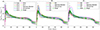Fig. 1.

Bolometric LCs for a grid of models with CSM radii of 1.5 × 10¹⁴ cm (a; left), 6 × 10¹⁴ cm (b; middle), and 10¹⁵ cm (c; right). The observational data are taken from Bersten et al. (2024), Martinez et al. (2024), Singh et al. (2024), and Zimmerman et al. (2024).

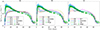Fig. 2.

Pseudo-bolometric LCs for a grid of models with CSM radii of 1.5 × 10¹⁴ cm (a; left), 6 × 10¹⁴ cm (b; middle), and 10¹⁵ cm (c; right). The observational data are taken from Hiramatsu et al. (2023), Hsu et al. (2024), and Singh et al. (2024).

In our figures, we collected data for SN 2023ixf from different studies: Hiramatsu et al. (2023), Teja et al. (2023), Singh et al. (2024), Bersten et al. (2024), Martinez et al. (2024), Li et al. (2024), Hsu et al. (2024). We choose MJD = 60 082.788 as a reference point (Li et al. 2024), which indicates time ‘0’ in all figures in our paper. The so-called ‘explosion epoch’ or ‘time of explosion’ for SN 2023ixf is defined as the average between the first detection and the last non-detection and corresponds to MJD = 60 082.75 (Hosseinzadeh et al. 2023). Other ways of estimating the ‘explosion epoch’ include fitting of the early LC with a power-law and choosing the ‘explosion time’ as the time when the flux equals zero (Zhang et al. 2023). Nevertheless, these methods, being dependent on the limiting magnitude or epoch of the last non-detection, do not necessarily reflect the physical meaning of the time of the actual explosion. To be physically precise, the ‘explosion epoch’ corresponds to the onset of an explosion, that is the moment when the SN shock is successfully launched in the vicinity of a stellar core, starting its acceleration onwards. The shock propagates to the edge of the star during t_sbo = R_prog/v_sh, where v_sh ∼ 10 000 km s⁻¹ is the shock velocity, which equals 0.6 days for a progenitor similar to our ‘bare’ model with R_prog = 700 R_⊙. It means that the first photons can be detected 0.6 days after the explosion, consequently, the actual time of the explosion and observationally derived ‘time of explosion’ might be different. By default, time ‘0’ in STELLA simulations corresponds to the moment when the thermal energy is injected in the innermost layers of the ejecta. This means that it is close to the actual beginning of the explosion. Our CSM−interaction models consist of an artificially constructed CSM, and therefore the models require some time to adjust to an equilibrium structure according to the underlying set of equations. This means that the first day or so in the LC evolution might be unphysical. Therefore, there is some degree of freedom to shift different models to a different time, possibly within 2–11 days, to match the observations, in which one to two days account for the nonphysical part of a synthetic LC.

3.1. Light curves of the bare progenitor

Figures 1a and 2a show the LC for the bare progenitor, and we begin with a discussion of the properties of this LC.

Our goal was to build a progenitor and simulate its explosion with an energy that is consistent with the explosion energies derived from observations of SN remnants and with the neutrino-engine-driven and first-principle multi-dimensional CC simulations that we mentioned in Sect. 1. The resulting LC of our bare model, which does not have a CSM, with an energy of 0.7 foe matches the plateau phase of SN 2023ixf LC. Regarding the ejecta mass and the explosion energy, our result is in good agreement with the conclusions of Hsu et al. (2024), who explained SN 2023ixf as an explosion of a massive star above 15 M_⊙ that underwent an intense mass-loss phase and massive fallback, retaining a low mass of hydrogen-rich ejecta, and that had an energy of 0.5–0.7 foe. The progenitor radius in their self-consistent simulations, which followed the progenitor variability, is larger than the radius we set artificially in our input model, namely ≥950 R_⊙ instead of 700 R_⊙ for our model. Moreover, our progenitor model is not a self-consistently calculated stellar evolution model; therefore, we cannot also deduce the initial mass of the progenitor. These are weak points in our study. The lower ejecta mass in Hsu et al. (2024) simulations was achieved also because of the high fallback mass, up to 3.6 M_⊙, happening after the successful explosion. In our simulations, there is no matter falling back to the gravitational central object. The reason is most likely a different density structure of the inner regions lying above the collapsing core.

With our experiment of reducing the energy of the explosion in combination with lowering the ejecta mass and extending the envelope, we show that the plateau luminosity and its duration can be similar to the LC obtained with a higher energy of 2–3 foe and a higher ejecta mass (Teja et al. 2023; Moriya & Singh 2024; Singh et al. 2024). Hence, instead of considering such high values, the LC of SN 2023ixf can also be explained by an explosion with a more common energy of less than 1 foe, which is more consistent with well-accepted values predicted by self-consistent neutrino-driven CCSN simulations and derived from observations.

The degeneracy of bolometric LCs of Type IIP was explored by Goldberg et al. (2019). The same behaviour of the bolometric LC can be reproduced by progenitors with significantly different structures and masses. For example, the ejecta mass and explosion energy may differ by a factor of two and still reproduce the same shape of a bolometric LC, which is consistent with the scaling relations by Arnett (1980) and Popov (1993):

$\begin{matrix} \begin{matrix} log L \sim - 1 / 2 log M - 0.8 log E + 2 / 3 log R \\ log t_{p} \sim 1 / 2 log M - 1 / 6 log E + 1 / 6 log R . \end{matrix} \end{matrix}$ $\begin{aligned} \begin{array}{l} \log L \sim - 1/2\, \log M - 0.8\, \log E + 2/3\, \log R \\ \log t_\mathrm{p} \sim 1/2\, \log M - 1/6\, \log E + 1/6\, \log R. \end{array} \end{aligned}$ (1)

The higher the ejecta mass the longer the plateau, the higher the energy the shorter the plateau, the larger the progenitor radius the longer the plateau; and vice versa: the lower the ejecta mass the shorter the plateau, the lower the energy the longer the plateau, and the smaller the radius, the shorter the plateau. In particular, the bolometric LC of SN 2023ixf can be a result of a high energy in combination with a high ejecta mass, or the other way around: a lower energy and a lower ejecta mass can yield the same result according to Eq. (1). Moreover, an estimate of the progenitor and CSM parameters might be misled if one uses either only bolometric or only pseudo-bolometric LCs. Strong constraints on the radius of the progenitor can break the degeneracy, which can be done, for example, by considering the colour-temperature evolution before the LC settles to the recombination phase (Nakar & Sari 2010; Shussman et al. 2016; Kozyreva et al. 2020a). Spectral modelling either for the photospheric phase or the nebular epoch definitely provides an additional constraint on the progenitor parameters (Jerkstrand et al. 2012; Dessart et al. 2013; Dessart & Jacobson-Galán 2023; Ferrari et al. 2024).

In conclusion, we managed to reproduce the LC of SN 2023ixf, namely, the duration of the plateau and its luminosity after the ‘interaction’ phase with an explosion powered by 0.7 foe.

3.2. Light curves of the progenitor with circumstellar matter

In Figs. 1 and 2, we show the bolometric and pseudo-bolometric LCs for the progenitor enshrouded by CSM extending to different radii: 1.5 × 10¹⁴ cm (models W12–W17), 6 × 10¹⁴ cm (models W1–W6) and 10¹⁵ cm (models W7–W11). The mass of this CSM ranges between 0.07 M_⊙ and 1.56 M_⊙ (see details in Table 2).

The model with a compact CSM can reproduce the bolometric peak but fails to reproduce the slope of the rising part of the SN 2023ixf LC. The CSM cases with a radius of 6 × 10¹⁴ cm and masses of 0.07 M_⊙ or 0.17 M_⊙ resemble the peak shape, but drop at day 10 and last not long enough, while the CSM cases with a radius of 10¹⁵ cm and masses of 0.07 M_⊙ and 0.17 M_⊙ match the peak and its width. The higher-mass CSM overestimates the luminosity of the peak and its width, because the diffusion time is longer for the higher ejecta mass. The preferable models are: W1, W2 (6 × 10¹⁴ cm, 0.17 M_⊙ and 0.3 M_⊙), and W8 and W7 (10¹⁵ cm, 0.17 M_⊙ and 0.3 M_⊙), if we base our analysis on the bolometric LC. Martinez et al. (2024) inferred a CSM mass of 0.02 M_⊙ while fitting the shape of their bolometric LC, although their LC has a very sharp, probably unrealistic, peak and is an outlier among others.

The rising part of the LCs corresponds to the phase when the shock wave propagates through the CSM. As the shock is radiation-dominated, it accelerates particles via radiation pressure ahead, developing the so-called ‘thermal tongue’ (Zel’dovich & Raizer 1967; Grassberg et al. 1971; Chevalier 1976). Radiative acceleration pushes matter ahead of the shock, which leads to the emergence of the flash-ionisation features.

While looking at pseudo-bolometric LCs (Fig. 2), it is obvious that none of the models with the compact CSM matches the observations because of a flux deficit before day 20, which accounts for interaction. The models with R_CSM = 6 × 10¹⁴ cm can be considered matching the peak pseudo-bolometric luminosity of SN 2023ixf if the CSM mass is 0.55 M_⊙, 0.85 M_⊙ or 1.56 M_⊙. However, the slope of the rising part is shallower and the ‘interaction’ bump is narrower than that of SN 2023ixf. The models with R_CSM = 10¹⁵ cm and CSM mass of 0.3 M_⊙, 0.55 M_⊙, and 0.83 M_⊙ match the pseudo-bolometric LC of SN 2023ixf reasonably well.

There is some degree of discrepancy between the estimate of the CSM mass via bolometric LCs and pseudo-bolometric LCs. The lower mass of the CSM required to match the bolometric luminosity may be explained by the fact that our synthetic bolometric LC is an integration of the flux over the entire electromagnetic spectrum, whereas the ‘observed’ bolometric luminosity is a sum of the fluxes in a certain set of broad bands with additional components such as bolometric corrections and other adjustments. Therefore, the estimate based on the pseudo-bolometric LC is more appropriate, although the comparison in broad bands can be more reliable, and we discuss this below.

3.3. Broadband light curves

In Figs. C.1, C.2, C.3, C.4, C.5, and C.6 we show broadband LCs for our models. As concluded above, the models with the compact CSM are ruled out because of the flux deficit at earlier time (before day 20), which is also seen in broad bands. Therefore, we show models W12–W17 in Figs. C.4 and C.5 only for illustrative purposes. Otherwise, we concentrate our analysis on our models W1–W11.

The plateau part of the LCs matches the observed LC of SN 2023ixf reasonably well, at least not worse than in Bersten et al. (2024) or Moriya & Singh (2024). Although the flux in the u-band an z-band is overestimated in all models on the plateau compared to the observed one in SN 2023ixf, agreement in broad bands is acceptable. This means that our progenitor model, which determines the behaviour of the plateau, is suitable to mimic the structure of the star before the CC.

For the interaction part, none of the CSM structures can reproduce the behaviour of SN 2023ixf in all broad bands simultaneously. However, there are certain preferences for models: W10 and W11 match the observed LCs in a larger number of broad bands, which means that more extended, 10¹⁵ cm, and more massive, 0.55–0.85 M_⊙, CSM cases suit SN 2023ixf better. Models W4, W7, W8, and W9 are deemed to be appropriate, too. We note that studies by Hiramatsu et al. (2023) based their analysis on pseudo-bolometric and bolometric LCs. Using such data, however, can be ambiguous, and therefore their approach may not ultimately discriminate for the best-fit case because of the inherent difficulties in comparing wave-band integrated data from observational analysis with results from theoretical LC modelling.

To justify our choice of the best-fit models, we conducted a statistical analysis. We chose the Spearman correlation method to differentiate between models. To do so, we combined all available observational data in each band into a single array, and calculated Spearman correlation coefficients for each model in all bands. We processed all models within a time window between day 0 and day 30, without considering correlations for the ‘plateau’ phase, because the progenitor model was built specifically to well reproduce the plateau length and luminosity. Models W2, W3, W7, W8, W10, and W11 have the largest correlation coefficients, between 0.7 and 1. This result agrees with our assessment we made by simple eye inspection.

None of the models has sufficient flux in the z-band to reproduce the z-magnitude of SN 2023ixf during the first 30 days. The underestimated flux in red bands in combination with overestimated flux in blue bands can indicate that the colour temperature in our models is somewhat too high to explain the colours of SN 2023ixf. It might be that a slightly higher metallicity in our input progenitor could suppress the blue flux and redistribute it to the redder part of the spectrum. Another possibility might be connected to the degree of mixing of radioactive nickel ⁵⁶Ni, according to which the SN ejecta at larger radii have a higher fraction of nickel in comparison to centrally concentrated nickel. Nickel together with other iron-group elements has large line opacities, which in turn, effectively redistribute blue flux into redder wavelengths (Pinto & Eastman 2000; Kasen 2006; Kozyreva et al. 2020b).

3.4. The first five hours of SN 2023ixf

Li et al. (2024) achieved to capture emission from SN 2023ixf already during the first hours after confirmed non-detection (Fig. 3) and 22.5 hours, what means almost one day, before the discovery observation of the SN by Itagaki (2023). These observations are unique and provide extremely valuable information of the very compact CSM surrounding the surface of the progenitor or of an outermost, puffy atmosphere of the progenitor. Therefore they indicate an unusual dynamical activity happening a few hours before or after the CC. Therefore, we pay special attention to the first five hours of SN 2023ixf LC and analyse this phase in more detail.

Our best-fit models, those with CSM of 6 × 10¹⁴ cm and 10¹⁵ cm, have a slope that is shallower than SN 2023ixf and slightly overestimates the flux in this earliest epoch, which is not seen in Figs. 1, 2, and C.1–C.6 because the plots cover 100 days of the LC evolution. Models W12–W17 with the more compact CSM of 1.5 × 10¹⁴ cm have a sharper rise to the SN LC peak but suffer from the flux deficit around the peak. Our model W17 with a CSM mass of 1.56 M_⊙ extending to 1.5 × 10¹⁴ cm reproduces the earlier LC of SN 2023ixf. However, 1.56 M_⊙ of CSM in this case have a pronounced impact on the plateau duration, making it 10 days longer². The immediate explanation of SN 2023ixf then can be that the progenitor was not surrounded with a single type of CSM but had an asymmetric density profile, such as, more extended along one axis and less extended along another axis. An asymmetric compact CSM around the progenitor of SN 2023ixf was in fact confirmed by spectropolarimetry observations (Vasylyev et al. 2023; Singh et al. 2024). It might be that a combination of different CSM structures contributes to the overall LC gradually, in other words, photons from the shock propagating through the more compact CSM break out earlier, then photons from the shock propagating along the more extended CSM dominate the LC a few hours later. We also tried more compact CSM cases with radii of 10¹⁴ cm and smaller and lower masses of 0.001–0.01 M_⊙. However, such structures of the CSM lead to a steeper slope and thus cannot be considered as successful in reproducing the early phase of the LC of SN 2023ixf.

In any case, the early LC rise, which appeared like a flux excess in the analysis of Li et al. (2024) cannot be satisfactorily reproduced by any of our tested SN models with CSM. Instead, in 1D models it can only be explained by an additional thin layer or shell that lies right on top of the progenitor and has a substantially higher density than the ambient CSM (the density at the inner edge of the CSM is between ∼3 × 10⁻¹² g cm⁻³ and 10⁻⁹ g cm⁻³, whereas the density at the inner edge of the shells we consider below is taken to be 10⁻⁸ g cm⁻³). We note that shocking such a layer with an energy equivalent to the explosion energy will lead to a very sharp rise to a high-luminosity feature. In order to reduce this luminosity spike, the thin shell or a compact CSM should be unreasonably massive, far above 1 M_⊙, like our W17 model with the CSM mass of 1.56 M_⊙. The higher mass would make the rise shallower, however, meaning that the LC is less suitable for matching the early rise. This is in accordance with the inverse dependence of the shock-breakout luminosity on the mass and its linear dependence on energy. Thus, we conclude that the energy powering the five-hour feature has to be lower than 0.7 foe.

Therefore, we tested another hypothetical scenario, assuming that the additional shell around the progenitor radiates energy in an expansion that is driven by much less energy. To this end we calculated a set of independent models as an alternative attempt to reproduce the initial LC rise as required by the observations in the time window of five hours before the first official discovery of SN 2013ixf. Specifically, we constructed a variety of shell models with masses between 0.5 M_⊙ and 1 M_⊙, inner radius of 700 R_⊙, and outer radii of 800 R_⊙, 900 R_⊙, and 1000 R_⊙. To build these shell models, we used the outer mass zones of the progenitor structure (our base model ‘bare’) including their chemical composition and scaled the density and radius to the desired values, while keeping the inner density at 10⁻⁸ g cm⁻³. We mapped the shell models into STELLA and followed their evolution after injecting energies between 0.0005 foe and 0.02 foe, or 5 × 10⁴⁷ erg and 2 × 10⁴⁹ erg, into the innermost computational grid zones of the shells. In Table 3 we list only those combinations which, from our point of view, yield the best match of the first 5-hour phase of SN 2023ixf.

Table 3.

Shell model parameters.

In Fig. 3 we present the resulting LCs of the expanding shells. We note that these models do not include the combined system of ‘progenitor+shell+CSM’, but consist exclusively of a shell that is gravitationally unbound from the progenitor. Additionally, we show the CSM model W17, which has a LC appropriate for SN 2023ixf (see above). The radiation in the shell models is powered by the injected energy, which triggers a shock propagating across the shell and causes radiation streaming away from the shock front. The synthetic LCs in g, V, and r broad bands are shown in comparison to those of SN 2023ixf. All shell-models and W17 reproduce the V-band LC of SN 2023ixf, while suffering a flux excess in the g band and a flux deficit in the r band. Nevertheless, our W17 wind-model includes 1.56 M_⊙ of CSM within 1.5 × 10¹⁴ cm, which we consider being too massive to be realistic. It might be that the large amount of dust reported by Niu et al. (2023) suppresses flux in the bluer bands such as the g-band (see also Kilpatrick et al. 2023; Pledger & Shara 2023; Qin et al. 2024; Van Dyk et al. 2024; Xiang et al. 2024). In addition to Fig. 3, we show V-band LCs for our shell-models together with the best-fit wind-models in Appendix D.

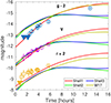Fig. 3.

Light curves of g, V, and r for a CSM model W17 with a compact CSM (1.5 × 10¹⁴ cm, 1.56 M_⊙), and shell models: ‘Shell1’, ‘Shell2’, and ‘Shell3’ with an inner radius of 700 R_⊙, outer radii of 1000 R_⊙, 900 R_⊙, and 800 R_⊙, masses of 0.9 M_⊙, 1 M_⊙, and 0.5 M_⊙, and injected energies of 0.01 foe, 0.02 foe, and 0.0185 foe, respectively. The observational data are taken from Li et al. (2024) and are shown by circles. The triangles indicate non-detection and are also from Li et al. (2024).

It would overstate the case if we claimed that our models provide a good fit to the data, but the shell models at least follow the LC slopes in the early phase of SN 2023ixf. Therefore, we conclude that a small part of the outermost envelope of the progenitor could have been swept out by a burst of energy of about 0.01–0.02 foe a few hours before the main shock from the explosion reached the edge of the progenitor. The mass ejection of the shell could also be asymmetric. The proposed shell ejection is in agreement with other studies on SN 2023ixf claiming that the progenitor’s mass-loss rate increased rapidly while the star was approaching its CC (Bostroem et al. 2024).

In our hypothetical scenario, we assume that an additional energy deposition happens in the outermost layers of the progenitor almost simultaneously with the main explosion, what means shortly before the breakout of the SN shock from the stellar surface. If the corresponding injection of a low amount of energy occurs at a smaller radius somewhere in the interior of the pre-collapse star, the weak shock formed by that will propagate through the rest of the envelope only over days (see Tsuna et al. 2024). This means that a close temporal correlation of shell ejection and SN outburst would require quite some fine-tuning in order to avoid the shell being expelled much too early or there not being enough time for the weak shock to reach the edge of the stellar envelope before the main shock from the explosion catches up with it. In the next section we discuss some possible origins of the assumed pre-SN outburst and its corresponding injected energy, and the connection to the required CSM around the progenitor of SN 2023ixf.

4. Origin of the circumstellar matter around SN 2023ixf progenitor and origin of the pre-supernova outburst

As discussed above, there are three important ingredients required to reconstruct the LC appearance of SN 2023ixf and, in turn, to explain the physics and nature of this transient. These are: (1) the progenitor structure, namely, its final mass just before the CC, which is about 7.4 M_⊙ in our model – and, corresponding to it, the ejecta mass of about 6 M_⊙ – as well as its radius of about 700 R_⊙; (2) the CSM structure: a mass of about 0.55 M_⊙ with a radius of 10¹⁵ cm; and (3) the shell of stellar material ejected with energy of about 0.01 foe to explain the steep initial rise of the LC during the first five hours. In the following, we attempt to sketch possible scenarios to fulfil these requirements.

4.1. Binary nature

To match the plateau phase of SN 2023ixf, we constructed a progenitor with a final mass of 7.4 M_⊙, which is lower than the final mass of stellar models with an initial mass of 10 − 20 M_⊙ at solar metallicity (Hirschi et al. 2004). This means that the progenitor had to lose more mass than the steady wind mass loss predicts. One of the most probable channels is to consider a star within a binary system so that the outermost layers are transferred via Roche-Lobe overflow (RLOF) to a companion (Laplace et al. 2021; Klencki et al. 2022; Ercolino et al. 2024). The mass transfer rate can be so high that the companion is not able to accrete this amount of mass, and a circumbinary disc is formed, in turn, extending to radii a few times the orbital separation. It is well known that extra mass loss due to binary interaction plays a significant role for stripped-envelope SNe of Type Ibc (Yoon et al. 2012; Fox et al. 2022).

Hsu et al. (2024) discussed that there should be two processes or episodes that led to intensive mass loss of the progenitor system of SN 2023ixf: the first episode is responsible for stripping the progenitor to reduce its mass during the earlier phases of evolution, and the second episode via which the CSM was formed. The progenitor is supposed to lose a high fraction of its hydrogen-rich envelope during earlier phases of evolution. For example, if a non-rotating star is 15 M_⊙ initially, it loses 2.4 M_⊙ via wind mass loss (Sukhbold et al. 2016). However, the progenitor of SN 2023ixf had to have 7.4 M_⊙ before its CC, and assuming it was 15 M_⊙ at the beginning, it had to lose 7.6 M_⊙, which means that an extra 5 M_⊙ should be removed during its evolution, including the red supergiant (RSG) phase. Similarly, a 10 M_⊙ star loses 0.3 M_⊙ via its wind and is required to lose another 2.3 M_⊙ to be a suitable progenitor for SN 2023ixf. As shown in the literature, increasing the mass-loss rate by a fixed factor might not necessarily help (Meynet et al. 1994), since the population of RSGs and hydrogen-depleted stars will not be consistent with observations.

To conclude, it is likely that the progenitor of SN 2023ixf was part of a binary and had lost its mass both via wind mass loss and binary interaction. The CSM may represent the matter that escaped from the primary during core carbon, neon, and oxygen burning in a dynamically unstable regime, or in a phase of super-thermal accretion by the secondary (i.e. the mass transfer from the primary happened at a high rate on a time scale shorter than the Kelvin–Helmholtz, or thermal, time scale). This matter remained trapped in the system and could form the CSM (Kippenhahn & Meyer-Hofmeister 1977; Lau et al. 2024). We discuss more details of some possible CSM formation scenarios in the next section.

4.2. Pre-supernova outburst and origin of circumstellar matter

According to our analysis, the steep rise in the SN 2023ixf LC during the first hours after confirmed non-detection (see Fig. 3) might point to a low-energy pre-SN outburst. Our approximate model considers a shell of matter ejected from the progenitor about half a day before the shock breaks out from the surface of the progenitor. This outburst could be correlated with the SN or of uncorrelated nature.

Uncorrelated nature means that the CC and the mass ejection happen independently of each other and are not connected. In this case, the mass ejection is a result of dynamical activity going on in extended RSGs. On the one hand, these stars possess convective envelopes with convective plumes encompassing the entire hydrogen-rich envelope of the star (Chiavassa et al. 2009; Kravchenko et al. 2018; Chiavassa 2022; Goldberg et al. 2022a; Singh et al. 2023). On the other hand, sound waves and gravity waves arising from convective burning activity in the progenitor’s core might transmit an energy of 10⁴⁸ erg into the envelope during the final years before the CC (Quataert & Shiode 2012; Wu & Fuller 2021). This epoch corresponds to the nuclear burning stages of core-neon and core-oxygen burning, which last a few years. The thermal timescale of the envelope is the Kelvin–Helmholtz time and is equal to a few hundred years, meaning that the envelope cannot respond immediately to nuclear and dynamical processes in the core evolving on a shorter timescale. The energy released via core and shell burning is the source of energy for exciting the internal gravity waves. Merging sound waves and damped gravity waves result in outgoing acoustic waves and ultimately in shock waves that could initiate an expansion of the envelope or/and an ejection of outermost layers (Quataert et al. 2016; Fuller 2017; Fuller & Tsuna 2024) and the formation of an extended CSM. We note that such a long-lasting, extensive mass-loss phase over several final years of the progenitor’s evolution might provide the CSM needed to explain the main LC of SN 2023ixf. Regarding the LC feature that is observed during the first hours, mass ejection caused by stochastic processes such as convection or strong gravity-wave activity might also be responsible. However, we emphasise that there would have to be a particular shell ejection just half a day before the main shock breaks out.

A mass ejection as an extreme case of an intensive mass loss during the latest evolutionary stages can be a result of an amplified regular wind mass loss. The known RSG wind mass-loss rates are about 10⁻⁶ M_⊙ yr⁻¹ (Beasor & Davies 2018), which is not sufficient for the formation of the CSM needed for SN 2023ixf. However, wind mass loss can be increased by pulsations (Wood et al. 1983; Weiler et al. 1992; Heger et al. 1997; Yoon & Cantiello 2010), which massive stars are predisposed for, and the SN 2023ixf progenitor, too (Kilpatrick et al. 2023; Soraisam et al. 2023; Hsu et al. 2024).

Alternatively, the mass ejection might also be correlated with the stellar collapse taking place in the deep interior of the stellar core. In Sect. 4.2 we considered shell models that match the early SN 2023ixf LC. These models include a shell with a mass of 0.5–1 M_⊙ and a width of 100–300 R_⊙ ejected with the energy of about 0.01 foe.

Our numbers for mass (∼0.5 M_⊙) and energy (0.01 foe) of the pre-SN outburst are consistent with results deduced from observations (Strotjohann et al. 2021) and a theoretical approach (e.g. Matsumoto & Metzger 2022). However, they represent upper limits for these parameters, since the eruption might be asymmetric. It is possible that another outburst with a lower energy and lower luminosity occurred before the detection of SN 2023ixf and remained undetected, because several studies reported non-detection of outbursts at the location of SN 2023ixf for many years before the SN was detected (Flinner et al. 2023; Neustadt et al. 2024; Ransome et al. 2024). There are SNe for which precursor emission was detected years before the terminal explosion (see, e.g., Jacobson-Galán et al. 2022). For instance, Tinyanont et al. (2022) suggested that a CSM around SN 2020fqv originates from an outburst that happened 200 days before the CC with energy of 5 × 10⁴⁶ erg, which is three orders of magnitude lower than our estimate. The matter stripped off during years prior to the CC indeed can be responsible for the formation of a CSM required for shaping the appearance of SN 2023ixf, but not for the matter ejected within a fraction of day before the explosion.

The shock formed in the shell reaches the outer edge in 1, 0.6, 0.4 days for our models ‘Shell1’, ‘Shell2’, and ‘Shell3’, correspondingly. This means that the shells did not have time to expand, keeping its original radius. By this time the main shock reaches the edge of the progenitor and starts propagating through the shell material. By the time when the main shock reached the shell’s edge, the shell expanded to another 100–200 R_⊙ and represented a very compact CSM, meaning that the shell is unlikely to have a significant effect on the resulting LC, as we showed in Sect. 3.2 for models W12–W17 with a compact CSM. The shell matter is ionised and optically thick; therefore, the radiation from the front of the main shock is not seen until it breaks out from the shell and continues moving through the lower-density CSM. The LC is formed as a combination of the flux from the shell ejection with its energy of 0.01–0.02 foe and from the SN shock that was initiated by the release of 0.7 foe in the explosion mechanism.

We emphasise that aspherical mass ejection by 3D asymmetries of the SN explosion as well as any deviation of the progenitor from ideal sphericity, caused by large-scale convective plumes or the outward propagation of gravity waves, may play an important role in shaping the overall LC. The visible SN emission includes flux contributions from different components of the ejecta, thus probing larger volumes and deeper layers as time progresses.

4.3. Supernova precursors as probes of new physics

In this section we highlight that early-time observations of SN explosions, such as those of SN 2023ixf analysed in this work, might offer a promising avenue for exploring physics beyond the Standard Model. Conclusions on such new physics, however, are reasonable and evidential only if the effects of asymmetries in the mass distribution of the progenitor envelope, explosion ejecta, and of the matter in the closest vicinity of the pre-explosion star are well understood.

SNe, particularly SN 1987A (due to its registered neutrino signal), have been routinely used to impose some of the strongest constraints on new particles, such as axions, dark photons, sterile neutrinos, etc. (Raffelt 1996; Caputo & Raffelt 2024). The underlying principle is that, even though exotic particles interact only weakly with Standard Model particles, they can still be produced in large numbers within the dense and hot cores of SNe, much like neutrinos. Depending on their masses and couplings strengths, these particles can give rise to distinctive observational signatures, potentially leading to their discovery or imposing limits on their existence. To illustrate this idea, we focus on a specific example: axion-like particles coupled to photons, which are among the most studied hypothetical particles nowadays (Mirizzi et al. 2016; Di Luzio et al. 2020; Caputo & Raffelt 2024; O’Hare 2024; Safdi 2024). While here we use axions³ as a jumping-off point, the general framework applies, with appropriate modifications, to a wide range of other exotic candidates.

Consider an axion particle with mass m_a and a coupling to photons G_aγγ. This latter sets the strength of the interaction of axions and ordinary photons, via the interaction term ℒ_a ⊃ −G_aγγa E · B, where a is the axion field and E,B are the electric and magnetic fields, respectively. Thanks to this interaction term, axions get produced in the SN core either via the Primakoff effect, where photons get converted into axions in the electric field of ambient ions/protons, γ + Ze → Ze + a, or via photon coalescence, γ + γ → a. If the axion mass is above ∼50 MeV or so, coalescence is the most important channel; otherwise, the Primakoff effect dominates.

After being produced in the inner part of the star, axions travel outwards relativistically (or semi-relativistically, if the mass is very large) and their fate crucially depends on their mean free path to decay back into a pair of photons, λ_{a → γγ}. This mean free path is similar to the radiative decay of pions and reads as

$\begin{matrix} λ_{a \to γ γ} = \frac{64 π}{G_{a γ γ}^{2}} \frac{\sqrt{ω_{a}^{2} - m_{a}^{2}}}{m_{a}^{4}} ≃ \frac{4 \times 10^{13}}{G_{9}^{2}} \frac{ω_{100}}{m_{10}^{4}} cm, \end{matrix}$ $\begin{aligned} \lambda _{a \rightarrow \gamma \gamma } = \frac{64 \pi }{G_{a\gamma \gamma }^2}\frac{\sqrt{\omega _a^2-m_a^2}}{m_a^4} \simeq \frac{4 \times 10^{13} }{G_9^2}\frac{\omega _{\rm 100}}{m_{10}^4}\,\mathrm{cm}, \end{aligned}$ (2)

where G₉ ≡ G_aγγ/10⁻⁹ GeV⁻¹, ω₁₀₀ ≡ ω_a/100 MeV is the particle energy of the axions, m₁₀ ≡ m_a/10 MeV, and where in the last part of the equation we have taken the relativistic limit ω_a ≫ m_a for simplicity.

Thus, if axions are very light and/or have a very small coupling, they can freely escape from the star, λ_{a → γγ} ≫ R_* (where R_* is stellar radius), effectively providing a new cooling channel. The presence of an extra cooling channel would make the SN core cooling down faster, in turn shortening any associated neutrino signal. This is in essence the ‘cooling argument’ that was applied to SN 1987A almost 50 years ago (Turner 1988) (although the first papers on the subject studied the axion coupling to nucleons, rather than photons). As a rough estimate, if the axion luminosity L_a for a given point in parameter space – defined by mass and coupling – is comparable to that of neutrinos around one second after core bounce, then that point in the parameter space is excluded. This is the so-called ‘Raffelt criterion’ (Raffelt 1996). This limit corresponds to the solid blue line in Fig. 4, obtained using the simulations of Bollig et al. (2020).

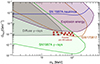Fig. 4.

Axion parameter space. All shaded regions are excluded by one or more astrophysical probes. Specifically, the region above the blue line is excluded by the duration of the neutrino signal from SN 1987A (Raffelt 1996). The purple region is excluded by the explosion energies of Type IIP SNe (Caputo et al. 2022b), assuming a typical star with a radius of R_* = 5 × 10¹³ cm and a lower limit on the explosion energy of 0.1 foe. The grey region is constrained by measurements of the extragalactic background light (Caputo et al. 2022a), while the green region is excluded by the upper limit on the gamma-ray fluence from SN 1987A (Caputo et al. 2022a), as determined by GRS. The shaded orange region is instead in tension with X-ray observations of GW170817 event (Diamond et al. 2024). The red stars highlight points of the parameter space around which the axion’s mean free path is within ∼10¹² − 10¹⁴ cm and the energy deposition at such distances accrues to ∼0.01–0.1 foe.

Once axions escape the star, they can still decay into photons outside the progenitor envelope, producing gamma-ray signals. For example, if the mean free path is comparable or smaller than the distance to SN 1987A, d_1987A ≃ 51.4 kpc, strong constraints derive from the Gamma-Ray Spectrometer (GRS) on board the Solar Maximum Mission (SMM) satellite that operated 02/1980–12/1989. Photons from axions emitted by SN 1987A would have been picked up by this instrument, which instead set only upper limits on the photon fluence, thereby constraining the existence of axions (Jaeckel et al. 2018; Caputo et al. 2022a; Hoof & Schulz 2023), as indicated by the green region in Fig. 4. Interestingly, Müller et al. (2024) applied the same argument to SN 2023ixf using Fermi-LAT gamma-ray observations of the event to put constraints on smaller axion masses (given that SN 2023ixf took place at a greater distance than SN 1987A).

If instead λ_{a → γγ} is of cosmological size, then the main constraints come from the integrated signals of all past SNe. In fact, axions would create a cosmic background density analogous to the diffuse SN neutrino background (Ando & Sato 2004; Beacom 2010; Mirizzi et al. 2016; Kresse et al. 2021); then, when they decay, they contribute to the diffuse gamma-ray background. One can then use the extragalactic background light measured by a variety of missions (Ackermann et al. 2015), such as Fermi-LAT or SMM, to place complementary constraints on the axion parameter space (Caputo et al. 2022a), indicated in grey in Fig. 4.

So far we have described different observables which can constrain axions with λ_{a → γγ} ≫ R_*. What if instead λ_{a → γγ} < R_*? In this case, if R_NS < λ_{a → γγ} < R_* (where R_NS is the radius of the new-born neutron star), most of the electromagnetic energy is dumped within the progenitor star, contributing to the SN explosion energy, which thus provides a ‘calorimetric’ constraint on new particles (Falk & Schramm 1978). Such a constraint is particularly severe when applied to a SN population with particularly low explosion energies (Spiro et al. 2014; Pejcha & Prieto 2015; Goldberg et al. 2019), as recently suggested by Caputo et al. (2022b). When axions decay on route to energetic gamma-ray photons in the stellar interior, the photons get quickly absorbed by pair production on nuclei. The precise impact of this energy deposition is subtle: if the luminosity in axions is locally comparable or larger than the Eddington luminosity, then the energy deposited will directly accelerate the medium; otherwise, it will mostly heat the stellar matter. In either case, the energy deposited must be below approximately 0.1 foe to remain consistent with observations (Caputo et al. 2022b). This bound is shown as a purple shaded region in Fig. 4. The lower part of this curve up to masses of ∼200 MeV is determined by the condition λ_{a → γγ} ∼ R_IIP, where R_IIP = 5 × 10¹³ cm is the typical size of a progenitor of a SN IIP adopted in Caputo et al. (2022b). Axions with parameters below this curve, and with m_a ≲ 200 MeV, have a mean free path longer than 5 × 10¹³ cm and deposit an energy $0.1 foe \times {(G_{a γ γ} / G_{a γ γ}^{curve})}^{2}$ $0.1\,\mathrm{foe} \times (G_{a\gamma\gamma}/G_{a\gamma\gamma}^{\mathrm{curve}})^2$ , where $G_{a γ γ}^{curve}$ $G_{a\gamma\gamma}^{\mathrm{curve}}$ is the axion-photon coupling value at a given mass on the purple curve in Fig. 4. Furthermore, in a similar region of the axion parameter space (for slightly larger mean free path), it is also possible that the photons produced from axion decay form a fireball, which would then produce X-ray emission. Diamond et al. (2024) used X-ray observations of the GW170817/GRB 170817A event and excluded the region inside the orange curve in Fig. 4. Part of the region denoted by ‘SN1987A γ − rays” is actually excluded by an analogous argument about the production of X-ray, which should have been detected by the Pioneer Venus Orbiter (Diamond et al. 2023). Actually, one could use Chandra-ACIS and NuSTAR X-ray observations of SN 2023ixf (Chandra et al. 2024; Grefenstette et al. 2023) in a similar way.

It is important to notice that the gravitational binding energy of all layers outside the stellar core is at most some 0.01 foe in low-mass progenitors (see Table 1 of Stockinger et al. 2020), and orders of magnitude lower in the hydrogen envelope. Therefore, the small amount of energy deposited by axions can easily eject the stellar material. As an example, consider the red stars in Fig. 4. They identify axions with mass and coupling such that λ_{a → γγ} ∼ 10¹² − 10¹⁴ cm, and would deposit an energy of roughly ≳0.01 foe, when decaying. In summary, these axions would: get produced mainly via photon coalescence in the SN core, around r₀ ∼ 10 km; travel through the stellar envelope at the speed of light and deposit most of their energy at r₁ ∼ λ_aγγ, in a time $λ_{a γ γ} / c ≃ 1 h (λ_{a γ γ} / 10^{14} cm)$ $\lambda_{a\gamma\gamma}/c \simeq 1\,\mathrm{h} \Big( \lambda_{a\gamma\gamma}\, \Big/ 10^{14}\,\mathrm{cm}\Big)$ . On the other hand, the main shock forms close to the neutron star as neutrinos interact with the ambient matter, and it propagates to the surface of the star during a time $t_{sbo} = R_{*} / v_{sh} \sim 0.6 (R_{*} / 5 \times 10^{13} cm) (10^{9} {cm s}^{- 1} / v_{sh}) day$ $t_{\mathrm{sbo}}=R_* / v_{\mathrm{sh}} \sim 0.6\Big( R_*\, \Big/ 5 \times 10^{13}\,\mathrm{cm} \Big) \Big( 10^{9}\,\mathrm{cm\,s}^{-1}\,\Big/ v_{\mathrm{sh}} \Big)\,\mathrm{day}$ (approximate time between the formation of the shock and its breakout from the stellar surface), where v_sh is the shock velocity. This implies a time gap of roughly half a day between the energy deposition by axions and the shock breakout. For the parameter space around the red stars in Fig. 4, and more generally for parameters lying between the purple region and the green one, the axion energy would get deposited into the external shells studied in this work, at 700–1000 R_⊙. Even if the mean free path is larger than this (which means, for a fixed axion mass, smaller axion-photon couplings), the phenomenology may still be very interesting, with energy injected directly into the outer parts of the CSM around the progenitor star. The red stars in Fig. 4 are thus only a rough indication of the parameters for which we expect interesting features to arise in the SN LCs. Notice that the progenitor of SN 1987A was a blue supergiant star with a radius of (2 − 3)×10¹² cm (Woosley 1988). Therefore, for the mass and coupling of axions decaying inside the progenitor of SN 2023ixf, the axion decay would have happened outside the progenitor of SN 1987A, producing a detectable gamma-ray signal.

While the interesting region of the axion parameter space appears to conflict with bounds from GW170817 and SN1987A γ-ray observations, these two probes are based on single events (unlike the constraints from low-energy SNe or diffuse γ-ray observations). Since all astrophysical systems have inherent uncertainties – which can certainly affect bounds at a factor of a few levels – it is always preferable to have multiple probes covering the same region of parameter space.

The interaction of SN ejecta with the external layers of the star and the dense CSM can also produce high-energy cosmic rays, neutrinos and gamma-rays, a possibility recently studied by Kimura (2024). In fact, similar processes may take place also after the energy injection due to axions. Moreover, while in this section we discussed only the phenomenology of massive axions, which can decay on route into gamma-rays, another possibility is that much lighter particles can convert into gamma-rays in the magnetic fields of the progenitor stars (Manzari et al. 2024), if these fields are strong enough.

In summary, observations of SNe during their early hours can probe interesting regions for axions and other exotic particles. With advancements in transient observation facilities, a new path for investigating novel physics may soon open, encompassing an entire class of events rather than relying on single ones. However, as noted at the beginning of this section, properly characterising the injected energy is intricate, and all these possibilities deserve further detailed studies, which we leave for future work.

4.4. Supernova precursor by an aspherical shock breakout

Yet another explanation of the early steep rise of the LC of SN 2023ixf may be offered by the possibility that the explosion itself was intrinsically highly aspherical. One of the examples of an asymmetric explosion is the low-mass (9 M_⊙) model s9.0 that was evolved self-consistently in 3D from the onset of the neutrino-driven explosion until shock breakout (Stockinger et al. 2020). In such simulations the SN shock gets deformed during the first seconds after core bounce because neutrino heating triggers violent convective activity and buoyant mass flows in the post-shock volume. These initial ejecta asymmetries seed the growth of secondary Rayleigh–Taylor instability when the outgoing SN shock accelerates and decelerates around composition interfaces in the progenitor. The Rayleigh–Taylor plumes and associated Kelvin–Helmholtz instability lead to efficient mixing, by which heavy elements are carried outward and helium and hydrogen inward. Moreover, a large-scale asymmetry is imposed on the ejecta, which in extreme cases and under favourable conditions (as in the s9.0 model of Stockinger et al. 2020) can even produce a global deformation of the SN shock when propagating through the stellar envelope.

The deformed shock implies different velocities and energies in different directions, and therefore it reaches the stellar surface at different times. The shock breakout signal appears first in the direction of the fastest Rayleigh–Taylor plumes, and therefore the time between the shock breakout of the fastest plume and the slowest (or the average) parts of the SN shock is up to one day in model s9.0. Such intrinsic explosion asymmetries might concur with large-scale convective asymmetries in the RSG envelope and would thus stretch the breakout emission from the deformed shock over even longer times (Goldberg et al. 2022b) and produce precursor features (as searched for in SN 2024ggi; Shrestha et al. 2024). The case of a 9 M_⊙ explosion model investigated by Stockinger et al. (2020) might be special and future studies by 3D long-term neutrino-driven core-collapse simulations will have to show whether such effects can play a role for a wider variety of CCSNe.

Kozyreva et al. (2022) evaluated the s9.0 model for its direction dependent LCs (though only approximately by considering 1D transport with the STELLA code for different radial slices) and the corresponding 4π-equivalent explosion energies and showed that the breakout behaviour and inferred isotropic-equivalent explosion properties can vary significantly for different viewing angles. Since the observable emission depends on the observer position when the actual source is extremely non-spherical, our parametric 1D shell models might imply a misjudgment, that is overestimation, of the involved masses and energies.

Effects associated with asymmetric shock breakout can also be expected when the SN shock propagates through a rotationally deformed progenitor or magnetic field amplification in collapsing rotating stars causes magnetorotationally driven jets, jet-like collimated outflows, or choked jets that deposit their energy in expanding cocoons (e.g. Bisnovatyi-Kogan et al. 1976; Piran et al. 2019; Obergaulinger & Aloy 2021; Bugli et al. 2021; Powell et al. 2023). Although current stellar evolution and CCSN theory suggest that these phenomena are probably connected to special or extreme progenitor conditions (e.g. low metallicity, high angular momentum, strong magnetic fields) they might play a role for a wider spectrum of CC events (Piran et al. 2019; Soker 2024) and deserve further exploration.

5. Conclusions

In this study, we built a progenitor model for SN IIP 2023ixf, whose explosion with an energy of 0.7 foe is in agreement with the explosion energies of average Type IIP SNe according to observational and theoretical estimates. Our progenitor is based on a 10 M_⊙ stellar evolution model; however, we do not exclude that it could also be a massive star with a higher initial mass. We assumed that the progenitor has lost quite a large fraction of its hydrogen-rich envelope, more than it could strip via mass loss in a steady wind. We suggest that the higher mass loss was caused by binary interaction. We explain the peak of SN 2023ixf by the presence of a wind-like CSM, preferentially with a radius of 10¹⁵ cm and a mass of 0.3 − 0.83 M_⊙. This CSM might have formed as a result of stronger late mass loss caused by gravity waves driven by convective nuclear burning in the inner shells during the final years of the star’s evolution.

However, the early steep rise in the LC of SN 2023ixf, which is seen during the first five hours after observationally confirmed non-detection and prior to the SN discovery announced by Itagaki (2023), cannot be reproduced in our 1D simulations by CSM interaction of the SN shock in any of our otherwise well-fitting models. We therefore hypothesise that this earliest LC feature might represent precursor emission that could be connected to a pre-SN outburst in the outermost layers (0.5–1 M_⊙) of the progenitor driven by the deposition of a relatively small amount of energy of 0.01–0.02 foe near the surface of the hydrogen-rich envelope. Most likely, the particular outburst-causing event did not form the CSM needed to explain the peak of SN 2023ixf because there was no time for the ejected shell to reach the radius of 10¹⁵ cm. Within the established theoretical possibilities, the source of the energy injection into the hydrogen-rich envelope could be multi-dimensional phenomena, such as hydrodynamic instabilities in the shell-burning layers, gravity waves, pulsations, or mass ejection caused by large-scale convective plumes in the stellar envelope, which in turn could amplify the RSG wind. However, for all of these phenomena, an energy of 0.01–0.02 foe within a short period of time appears to be on the extreme side and hard to reach.

If the LC precursor is connected to the SN explosion itself, it may point to a highly asymmetric explosion. One possibility is that the SN shock was strongly deformed either because of a non-spherical progenitor, due to rapid rotation or 3D hydrodynamic activity, or because of convective post-shock plumes that deformed the shock and thus made it expand with significantly different velocities in different directions. Alternatively, the highly asymmetric explosion could have been caused by a low-energy jet that propagated (maybe even close to the speed of light) well ahead of the SN shock. Any such asymmetric explosion would have an impact on the early rise of the LC.

Sticking to the 1D setups considered in our present paper, yet another possibility is that an energy of 0.01–0.02 foe was released in the outermost regions of the envelope of the progenitor by the decay of exotic particles (e.g. axions or axion-like particles). Hypothetically, such particles can be produced simultaneously with neutrinos during the collapse of the stellar core and the cooling of the newly formed hot neutron star. However, this hypothesis requires a separate and thorough study and will be conducted in the future.

The kind of precursor emission analysed in the present study can be discovered during the first hours after the last observationally confirmed non-detection of the SN, and sensitive instruments⁴ and advanced software are needed to identify this signal and extract it from the rapidly swelling overall flux of radiation. Therefore, very high cadence observations – up to minutes – are required to fulfill this task. Operating and upcoming facilities dedicated to observing transients, such as LSST, or a wide network of small and medium telescopes (Bianciardi et al. 2023; Sgro et al. 2023) will be able to capture SNe at their birth, enhancing the potential to spot their precursor emission (Gagliano et al. 2025). Any discoveries regarding the precursor emission will help clarify what is happening at the surface of massive stars while their cores collapse. This is especially important for any upcoming close SN and ultimately for an SN in the Galaxy. Hence, the forthcoming advanced observational facilities will open a unique window to test and advance stellar astrophysics and to look for effects beyond the Standard Model of particle physics.

Data availability

The data computed and analysed for the current study are available via the link https://zenodo.org/doi/10.5281/zenodo.13936548.

¹

Kozyreva et al. (2014) showed that the LC of the bright SN 1992am resembles the LC of a low-mass pair-instability SN, that is, a thermonuclear explosion of a star with an initial mass of about 150 M_⊙. It therefore might not necessarily be a neutrino-driven CCSN.

²

We note that the LC of W17 is shifted by 11 days in Figs. 1, 2, and C.1–C.6 to match the plateau phase of SN 2023ixf.

³

In this work, we use the terms ‘axion’ and ‘axion-like particles’ interchangeably. More precisely, particle physicists typically use ‘axions’ to refer to pseudoscalar bosons that solve the strong Charge-Parity (CP) problem (Peccei & Quinn 1977; Weinberg 1978; Wilczek 1978) and primarily couple to nucleons, though they can also couple to photons. In this case, the particle’s mass and its coupling to photons are related. In contrast, ‘axion-like particles’ are pseudoscalar bosons that do not necessarily solve the strong CP problem, what means that mass of axion-like particle and photon coupling are independent parameters.

⁴

We note that the first data published in Li et al. (2024) were obtained by amateur astronomers with their small telescopes, such as 8-cm, 10-cm, 10.1-cm, 13-cm, 15-cm, 20-cm refractors (see details in Mao et al. 2023). Certainly, this was a fortunate success because of the unique proximity of SN 2023ixf.

Acknowledgments

We thank Kirill Sokolovskiy, Pavel Abolmasov, Steve Schulze, Nikolay Pavlyuk, Dmitriy Tsvetkov, Sergei Blinnikov, Edoardo Vitagliano for helpful discussions and comments, Avinash Singh, Brian Hsu, and Xiaofeng Wang for providing data of SN 2023ixf. PB is supported by the grant RSF 24-12-00141 for modelling supernova light curves with the STELLA code. AC is supported by an ERC STG grant (“AstroDarkLS”, grant No. 101117510). HTJ acknowledges support by the German Research Foundation (DFG) through the Collaborative Research Centre “Neutrinos and Dark Matter in Astro- and Particle Physics (NDM)”, grant No. SFB-1258-283604770, and under Germany’s Excellence Strategy through the Cluster of Excellence ORIGINS EXC-2094-390783311. The work by AM was conducted under the state assignment of Lomonosov Moscow State University.

References

Ackermann, M., Ajello, M., Albert, A., et al. 2015, Astrophys. J., 799, 86 [CrossRef] [Google Scholar]
Anderson, J. P., González-Gaitán, S., Hamuy, M., et al. 2014, ApJ, 786, 67 [Google Scholar]
Ando, S., & Sato, K. 2004, New J. Phys., 6, 170 [NASA ADS] [CrossRef] [Google Scholar]
Arnett, W. D. 1980, ApJ, 237, 541 [Google Scholar]
Asplund, M., Grevesse, N., & Sauval, A. J. 2005, in Cosmic Abundances as Records of Stellar Evolution and Nucleosynthesis, eds. T. G. Barnes, III, & F. N. Bash, Astronomical Society of the Pacific Conference Series, 336, 25 [Google Scholar]
Beacom, J. F. 2010, Ann. Rev. Nucl. Part. Sci., 60, 439 [NASA ADS] [CrossRef] [Google Scholar]
Beasor, E. R., & Davies, B. 2018, MNRAS, 475, 55 [NASA ADS] [CrossRef] [Google Scholar]
Bersten, M. C., Orellana, M., Folatelli, G., et al. 2024, A&A, 681, L18 [NASA ADS] [CrossRef] [EDP Sciences] [Google Scholar]
Bianciardi, G., Ciccarelli, A. M., Conzo, G., et al. 2023, TNSAN, 213, 1 [NASA ADS] [Google Scholar]
Bisnovatyi-Kogan, G. S., Popov, I. P., & Samokhin, A. A. 1976, Ap&SS, 41, 287 [NASA ADS] [CrossRef] [Google Scholar]
Blinnikov, S. I., Eastman, R., Bartunov, O. S., Popolitov, V. A., & Woosley, S. E. 1998, ApJ, 496, 454 [Google Scholar]
Blinnikov, S., Lundqvist, P., Bartunov, O., Nomoto, K., & Iwamoto, K. 2000, ApJ, 532, 1132 [NASA ADS] [CrossRef] [Google Scholar]
Blinnikov, S. I., Röpke, F. K., Sorokina, E. I., et al. 2006, A&A, 453, 229 [NASA ADS] [CrossRef] [EDP Sciences] [Google Scholar]
Blondin, S., Blinnikov, S., Callan, F. P., et al. 2022, A&A, 668, A163 [NASA ADS] [CrossRef] [EDP Sciences] [Google Scholar]
Bollig, R., DeRocco, W., Graham, P. W., & Janka, H. T. 2020, Phys. Rev. Lett., 125, 051104; Erratum: Phys. Rev. Lett. 126, 189901 (2021) [NASA ADS] [CrossRef] [Google Scholar]
Bollig, R., Yadav, N., Kresse, D., et al. 2021, ApJ, 915, 28 [NASA ADS] [CrossRef] [Google Scholar]
Bostroem, K. A., Pearson, J., Shrestha, M., et al. 2023, ApJ, 956, L5 [NASA ADS] [CrossRef] [Google Scholar]
Bostroem, K. A., Sand, D. J., Dessart, L., et al. 2024, ApJ, 973, L47 [NASA ADS] [CrossRef] [Google Scholar]
Bugli, M., Guilet, J., & Obergaulinger, M. 2021, MNRAS, 507, 443 [NASA ADS] [CrossRef] [Google Scholar]
Burrows, A. 2013, Rev. Mod. Phys., 85, 245 [Google Scholar]
Burrows, A., & Vartanyan, D. 2021, Nature, 589, 29 [CrossRef] [PubMed] [Google Scholar]
Burrows, A., Hayes, J., & Fryxell, B. A. 1995, ApJ, 450, 830 [NASA ADS] [CrossRef] [Google Scholar]
Burrows, A., Wang, T., & Vartanyan, D. 2024, ApJ, 964, L16 [NASA ADS] [CrossRef] [Google Scholar]
Caputo, A., & Raffelt, G. 2024, in 1st General Meeting and 1st Training School of the COST Action COSMIC WISPers, 1, 41 [NASA ADS] [Google Scholar]
Caputo, A., Raffelt, G., & Vitagliano, E. 2022a, Phys. Rev. D, 105, 035022 [NASA ADS] [CrossRef] [Google Scholar]
Caputo, A., Janka, H.-T., Raffelt, G., & Vitagliano, E. 2022b, Phys. Rev. Lett., 128, 221103 [CrossRef] [PubMed] [Google Scholar]
Chandra, P., Chevalier, R. A., Maeda, K., Ray, A. K., & Nayana, A. J. 2024, ApJ, 963, L4 [NASA ADS] [CrossRef] [Google Scholar]
Chevalier, R. A. 1976, ApJ, 207, 872 [NASA ADS] [CrossRef] [Google Scholar]
Chiavassa, A. 2022, in The Origin of Outflows in Evolved Stars, eds. L. Decin, A. Zijlstra, & C. Gielen (Cambridge, UK: Cambridge University Press), IAU Symposium, 366, 101 [NASA ADS] [Google Scholar]
Chiavassa, A., Plez, B., Josselin, E., & Freytag, B. 2009, A&A, 506, 1351 [NASA ADS] [CrossRef] [EDP Sciences] [Google Scholar]
Cox, D. P. 1972, ApJ, 178, 169 [NASA ADS] [CrossRef] [Google Scholar]
Dahlen, T., Strolger, L.-G., Riess, A. G., et al. 2004, ApJ, 613, 189 [NASA ADS] [CrossRef] [Google Scholar]
Dessart, L., & Jacobson-Galán, W. V. 2023, A&A, 677, A105 [NASA ADS] [CrossRef] [EDP Sciences] [Google Scholar]
Dessart, L., Hillier, D. J., Waldman, R., & Livne, E. 2013, MNRAS, 433, 1745 [NASA ADS] [CrossRef] [Google Scholar]
Di Luzio, L., Giannotti, M., Nardi, E., & Visinelli, L. 2020, Phys. Rept., 870, 1 [NASA ADS] [Google Scholar]
Diamond, M., Fiorillo, D. F. G., Marques-Tavares, G., & Vitagliano, E. 2023, Phys. Rev. D, 107, 103029; Erratum: Phys. Rev. D 108, 049902 [NASA ADS] [CrossRef] [Google Scholar]
Diamond, M., Fiorillo, D. F. G., Marques-Tavares, G., Tamborra, I., & Vitagliano, E. 2024, Phys. Rev. Lett., 132, 101004 [NASA ADS] [CrossRef] [Google Scholar]
Dong, Y., Sand, D. J., Valenti, S., et al. 2023, ApJ, 957, 28 [NASA ADS] [CrossRef] [Google Scholar]
Ebinger, K., Curtis, S., Fröhlich, C., et al. 2019, ApJ, 870, 1 [NASA ADS] [Google Scholar]
Ercolino, A., Jin, H., Langer, N., & Dessart, L. 2024, A&A, 685, A58 [NASA ADS] [CrossRef] [EDP Sciences] [Google Scholar]
Ertl, T., Janka, H. T., Woosley, S. E., Sukhbold, T., & Ugliano, M. 2016, ApJ, 818, 124 [NASA ADS] [CrossRef] [Google Scholar]
Falk, S. W., & Schramm, D. N. 1978, Phys. Lett. B, 79, 511 [NASA ADS] [CrossRef] [Google Scholar]
Fang, Q., Moriya, T. J., Ferrari, L., et al. 2025, ApJ, 978, 36 [NASA ADS] [CrossRef] [Google Scholar]
Ferrari, L., Folatelli, G., Ertini, K., Kuncarayakti, H., & Andrews, J. E. 2024, A&A, 687, L20 [NASA ADS] [CrossRef] [EDP Sciences] [Google Scholar]
Flinner, N., Tucker, M. A., Beacom, J. F., & Shappee, B. J. 2023, Res. Notes Am. Astron. Soc., 7, 174 [NASA ADS] [Google Scholar]
Fox, O. D., Van Dyk, S. D., Williams, B. F., et al. 2022, ApJ, 929, L15 [NASA ADS] [CrossRef] [Google Scholar]
Fuller, J. 2017, MNRAS, 470, 1642 [NASA ADS] [CrossRef] [Google Scholar]
Fuller, J., & Tsuna, D. 2024, Open J. Astrophys., 7, 47 [CrossRef] [Google Scholar]
Gagliano, A., Berger, E., Villar, V. A., et al. 2025, ApJ, 978, 110 [NASA ADS] [CrossRef] [Google Scholar]
Goldberg, J. A., Bildsten, L., & Paxton, B. 2019, ApJ, 879, 3 [Google Scholar]
Goldberg, J. A., Jiang, Y.-F., & Bildsten, L. 2022a, ApJ, 929, 156 [NASA ADS] [CrossRef] [Google Scholar]
Goldberg, J. A., Jiang, Y.-F., & Bildsten, L. 2022b, ApJ, 933, 164 [NASA ADS] [CrossRef] [Google Scholar]
Grassberg, E. K., Imshennik, V. S., & Nadyozhin, D. K. 1971, Ap&SS, 10, 28 [Google Scholar]
Grefenstette, B. W., Brightman, M., Earnshaw, H. P., Harrison, F. A., & Margutti, R. 2023, ApJ, 952, L3 [NASA ADS] [CrossRef] [Google Scholar]
Hamuy, M. 2003, ApJ, 582, 905 [NASA ADS] [CrossRef] [Google Scholar]
Heger, A., Jeannin, L., Langer, N., & Baraffe, I. 1997, A&A, 327, 224 [NASA ADS] [Google Scholar]
Herant, M., Benz, W., Hix, W. R., Fryer, C. L., & Colgate, S. A. 1994, ApJ, 435, 339 [NASA ADS] [CrossRef] [Google Scholar]
Hiramatsu, D., Tsuna, D., Berger, E., et al. 2023, ApJ, 955, L8 [NASA ADS] [CrossRef] [Google Scholar]
Hirschi, R., Meynet, G., & Maeder, A. 2004, A&A, 425, 649 [NASA ADS] [CrossRef] [EDP Sciences] [Google Scholar]
Hoof, S., & Schulz, L. 2023, JCAP, 03, 054 [CrossRef] [Google Scholar]
Hosseinzadeh, G., Farah, J., Shrestha, M., et al. 2023, ApJ, 953, L16 [NASA ADS] [CrossRef] [Google Scholar]
Hsu, B., Smith, N., Goldberg, J. A., et al. 2024, ApJ, submitted [arXiv:2408.07874] [Google Scholar]
Itagaki, K. 2023, TNSTR, 2023-39, 1 [NASA ADS] [Google Scholar]
Iwamoto, K., Mazzali, P. A., Nomoto, K., et al. 1998, Nature, 395, 672 [Google Scholar]
Jacobson-Galán, W. V., Dessart, L., Jones, D. O., et al. 2022, ApJ, 924, 15 [CrossRef] [Google Scholar]
Jacobson-Galán, W. V., Dessart, L., Margutti, R., et al. 2023, ApJ, 954, L42 [CrossRef] [Google Scholar]
Jaeckel, J., Malta, P. C., & Redondo, J. 2018, Phys. Rev. D, 98, 055032 [CrossRef] [Google Scholar]
Jäger, Z., Jr., Vinkó, J., Bíró, B. I., et al. 2020, MNRAS, 496, 3725 [CrossRef] [Google Scholar]
Janka, H.-T. 2012, Annu. Rev. Nucl. Part. Sci., 62, 407 [NASA ADS] [CrossRef] [Google Scholar]
Janka, H. T. 2017, in Handbook of Supernovae, eds. A. W. Alsabti, & P. Murdin (Cham: Springer), 1095 [CrossRef] [Google Scholar]
Janka, H.-T., & Kresse, D. 2024, Ap&SS, 369, 80 [NASA ADS] [CrossRef] [Google Scholar]
Janka, H. T., & Müller, E. 1996, A&A, 306, 167 [NASA ADS] [Google Scholar]
Jerkstrand, A., Fransson, C., Maguire, K., et al. 2012, A&A, 546, A28 [NASA ADS] [CrossRef] [EDP Sciences] [Google Scholar]
Kasen, D. 2006, ApJ, 649, 939 [NASA ADS] [CrossRef] [Google Scholar]
Kasen, D., & Woosley, S. E. 2009, ApJ, 703, 2205 [NASA ADS] [CrossRef] [Google Scholar]
Khabibullin, I. I., Churazov, E. M., Bykov, A. M., Chugai, N. N., & Sunyaev, R. A. 2023, MNRAS, 521, 5536 [NASA ADS] [CrossRef] [Google Scholar]
Kilpatrick, C. D., Foley, R. J., Jacobson-Galán, W. V., et al. 2023, ApJ, 952, L23 [NASA ADS] [CrossRef] [Google Scholar]
Kimura, S. S. 2024, arXiv e-prints [arXiv:2409.18935] [Google Scholar]
Kippenhahn, R., & Meyer-Hofmeister, E. 1977, A&A, 54, 539 [NASA ADS] [Google Scholar]
Klencki, J., Istrate, A., Nelemans, G., & Pols, O. 2022, A&A, 662, A56 [NASA ADS] [CrossRef] [EDP Sciences] [Google Scholar]
Kozyreva, A., Blinnikov, S., Langer, N., & Yoon, S. C. 2014, A&A, 565, A70 [NASA ADS] [CrossRef] [EDP Sciences] [Google Scholar]
Kozyreva, A., Nakar, E., & Waldman, R. 2019, MNRAS, 483, 1211 [NASA ADS] [CrossRef] [Google Scholar]
Kozyreva, A., Nakar, E., Waldman, R., Blinnikov, S., & Baklanov, P. 2020a, MNRAS, 494, 3927 [NASA ADS] [CrossRef] [Google Scholar]
Kozyreva, A., Shingles, L., Mironov, A., Baklanov, P., & Blinnikov, S. 2020b, MNRAS, 499, 4312 [NASA ADS] [CrossRef] [Google Scholar]
Kozyreva, A., Janka, H.-T., Kresse, D., Taubenberger, S., & Baklanov, P. 2022, MNRAS, 514, 4173 [CrossRef] [Google Scholar]
Kravchenko, K., Van Eck, S., Chiavassa, A., et al. 2018, A&A, 610, A29 [NASA ADS] [CrossRef] [EDP Sciences] [Google Scholar]
Kresse, D., Ertl, T., & Janka, H.-T. 2021, ApJ, 909, 169 [NASA ADS] [CrossRef] [Google Scholar]
Laplace, E., Justham, S., Renzo, M., et al. 2021, A&A, 656, A58 [NASA ADS] [CrossRef] [EDP Sciences] [Google Scholar]
Lau, M. Y. M., Hirai, R., Mandel, I., & Tout, C. A. 2024, ApJ, 966, L7 [NASA ADS] [CrossRef] [Google Scholar]
Li, G., Hu, M., Li, W., et al. 2024, Nature, 627, 754 [NASA ADS] [CrossRef] [Google Scholar]
Lovegrove, E., Woosley, S. E., & Zhang, W. 2017, ApJ, 845, 103 [NASA ADS] [CrossRef] [Google Scholar]
Mannucci, F., Della Valle, M., & Panagia, N. 2007, MNRAS, 377, 1229 [NASA ADS] [CrossRef] [Google Scholar]
Manzari, C. A., Park, Y., Safdi, B. R., & Savoray, I. 2024, Phys. Rev. Lett., 133, 211002 [NASA ADS] [CrossRef] [Google Scholar]
Mao, Y., Zhang, M., Cai, G., et al. 2023, TNSAN, 130, 1 [NASA ADS] [Google Scholar]
Martinez, L., Bersten, M. C., Anderson, J. P., et al. 2022, A&A, 660, A41 [NASA ADS] [CrossRef] [EDP Sciences] [Google Scholar]
Martinez, L., Bersten, M. C., Folatelli, G., Orellana, M., & Ertini, K. 2024, A&A, 683, A154 [NASA ADS] [CrossRef] [EDP Sciences] [Google Scholar]
Matsumoto, T., & Metzger, B. D. 2022, ApJ, 936, 114 [CrossRef] [Google Scholar]
Mazzali, P. A., Valenti, S., Della Valle, M., et al. 2008, Science, 321, 1185 [NASA ADS] [CrossRef] [Google Scholar]
Meynet, G., Maeder, A., Schaller, G., Schaerer, D., & Charbonnel, C. 1994, A&AS, 103, 97 [Google Scholar]
Mirizzi, A., Tamborra, I., Janka, H.-T., et al. 2016, Riv. Nuovo Cim., 39, 1 [NASA ADS] [Google Scholar]
Moriya, T. J., & Singh, A. 2024, PASJ, 76, 1050 [NASA ADS] [CrossRef] [Google Scholar]
Moriya, T. J., Subrayan, B. M., Milisavljevic, D., & Blinnikov, S. I. 2023, PASJ, 75, 634 [NASA ADS] [CrossRef] [Google Scholar]
Müller, B. 2016, PASA, 33, e048 [Google Scholar]
Müller, B., Heger, A., Liptai, D., & Cameron, J. B. 2016, MNRAS, 460, 742 [Google Scholar]
Müller, B., Melson, T., Heger, A., & Janka, H.-T. 2017, MNRAS, 472, 491 [Google Scholar]
Müller, E., Carenza, P., Eckner, C., & Goobar, A. 2024, Phys. Rev. D, 109, 023018 [CrossRef] [Google Scholar]
Nakar, E., & Sari, R. 2010, ApJ, 725, 904 [NASA ADS] [CrossRef] [Google Scholar]
Neustadt, J. M. M., Kochanek, C. S., & Smith, M. R. 2024, MNRAS, 527, 5366 [Google Scholar]
Niu, Z., Sun, N.-C., Maund, J. R., et al. 2023, ApJ, 955, L15 [NASA ADS] [CrossRef] [Google Scholar]
Obergaulinger, M., & Aloy, M. Á. 2021, MNRAS, 503, 4942 [NASA ADS] [CrossRef] [Google Scholar]
O’Hare, C. A. J. 2024, PoS, COSMICWISPers, 040 [Google Scholar]
Peccei, R. D., & Quinn, H. R. 1977, Phys. Rev. Lett., 38, 1440 [Google Scholar]
Pejcha, O., & Prieto, J. L. 2015, ApJ, 806, 225 [Google Scholar]
Pejcha, O., & Thompson, T. A. 2015, ApJ, 801, 90 [NASA ADS] [CrossRef] [Google Scholar]
Pinto, P. A., & Eastman, R. G. 2000, ApJ, 530, 757 [NASA ADS] [CrossRef] [Google Scholar]
Piran, T., Nakar, E., Mazzali, P., & Pian, E. 2019, ApJ, 871, L25 [NASA ADS] [CrossRef] [Google Scholar]
Pledger, J. L., & Shara, M. M. 2023, ApJ, 953, L14 [NASA ADS] [CrossRef] [Google Scholar]
Popov, D. V. 1993, ApJ, 414, 712 [NASA ADS] [CrossRef] [Google Scholar]
Powell, J., Müller, B., Aguilera-Dena, D. R., & Langer, N. 2023, MNRAS, 522, 6070 [NASA ADS] [CrossRef] [Google Scholar]
Qin, Y.-J., Zhang, K., Bloom, J., et al. 2024, MNRAS, 534, 271 [NASA ADS] [CrossRef] [Google Scholar]
Quataert, E., & Shiode, J. 2012, MNRAS, 423, L92 [NASA ADS] [CrossRef] [Google Scholar]
Quataert, E., Fernández, R., Kasen, D., Klion, H., & Paxton, B. 2016, MNRAS, 458, 1214 [NASA ADS] [CrossRef] [Google Scholar]
Raffelt, G. G. 1996, Stars as laboratories for fundamental physics: The astrophysics of neutrinos, axions, and other weakly interacting particles (Chicago : University of Chicago Press) [Google Scholar]
Ransome, C. L., Villar, V. A., Tartaglia, A., et al. 2024, ApJ, 965, 93 [CrossRef] [Google Scholar]
Safdi, B. R. 2024, PoS, TASI2022, 009 [Google Scholar]
Sgro, L. A., Esposito, T. M., Blaclard, G., et al. 2023, Res. Notes Am. Astron. Soc., 7, 141 [Google Scholar]
Shivvers, I., Modjaz, M., Zheng, W., et al. 2017, PASP, 129, 054201 [NASA ADS] [CrossRef] [Google Scholar]
Shrestha, M., Bostroem, K. A., Sand, D. J., et al. 2024, ApJ, 972, L15 [Google Scholar]
Shussman, T., Waldman, R., & Nakar, E. 2016, arXiv e-prints [arXiv:1610.05323] [Google Scholar]
Singh, A. P., Richards, A. M. S., Humphreys, R. M., Decin, L., & Ziurys, L. M. 2023, ApJ, 954, L1 [NASA ADS] [CrossRef] [Google Scholar]
Singh, A., Teja, R. S., Moriya, T. J., et al. 2024, ApJ, 975, 132 [CrossRef] [Google Scholar]
Soker, N. 2024, Open J. Astrophys., 7, 69 [Google Scholar]
Soraisam, M. D., Szalai, T., Van Dyk, S. D., et al. 2023, ApJ, 957, 64 [NASA ADS] [CrossRef] [Google Scholar]
Spiro, S., Pastorello, A., Pumo, M. L., et al. 2014, MNRAS, 439, 2873 [Google Scholar]
Stockinger, G., Janka, H. T., Kresse, D., et al. 2020, MNRAS, 496, 2039 [Google Scholar]
Strotjohann, N. L., Ofek, E. O., Gal-Yam, A., et al. 2021, ApJ, 907, 99 [NASA ADS] [CrossRef] [Google Scholar]
Sukhbold, T., Ertl, T., Woosley, S. E., Brown, J. M., & Janka, H. T. 2016, ApJ, 821, 38 [NASA ADS] [CrossRef] [Google Scholar]
Teja, R. S., Singh, A., Basu, J., et al. 2023, ApJ, 954, L12 [NASA ADS] [CrossRef] [Google Scholar]
Tinyanont, S., Ridden-Harper, R., Foley, R. J., et al. 2022, MNRAS, 512, 2777 [NASA ADS] [CrossRef] [Google Scholar]
Tsuna, D., Huang, X., Fuller, J., & Piro, A. L. 2024, ApJ, accepted [arXiv:2410.07055] [Google Scholar]
Turner, M. S. 1988, Phys. Rev. Lett., 60, 1797 [NASA ADS] [CrossRef] [Google Scholar]
Ugliano, M., Janka, H.-T., Marek, A., & Arcones, A. 2012, ApJ, 757, 69 [NASA ADS] [CrossRef] [Google Scholar]
Van Dyk, S. D., Srinivasan, S., Andrews, J. E., et al. 2024, ApJ, 968, 27 [NASA ADS] [CrossRef] [Google Scholar]
Vasylyev, S. S., Yang, Y., Filippenko, A. V., et al. 2023, ApJ, 955, L37 [NASA ADS] [CrossRef] [Google Scholar]
Weiler, K. W., van Dyk, S. D., Pringle, J. E., & Panagia, N. 1992, ApJ, 399, 672 [NASA ADS] [CrossRef] [Google Scholar]
Weinberg, S. 1978, Phys. Rev. Lett., 40, 223 [Google Scholar]
Wilczek, F. 1978, Phys. Rev. Lett., 40, 279 [Google Scholar]
Wood, P. R., Bessell, M. S., & Fox, M. W. 1983, ApJ, 272, 99 [Google Scholar]
Woosley, S. E. 1988, Astrophys. J., 330, 218 [NASA ADS] [CrossRef] [Google Scholar]
Wu, S., & Fuller, J. 2021, ApJ, 906, 3 [NASA ADS] [CrossRef] [Google Scholar]
Xiang, D., Mo, J., Wang, L., et al. 2024, Sci. China: Phys. Mech. Astron., 67, 219514 [NASA ADS] [CrossRef] [Google Scholar]
Yoon, S.-C., & Cantiello, M. 2010, ApJ, 717, L62 [NASA ADS] [CrossRef] [Google Scholar]
Yoon, S. C., Gräfener, G., Vink, J. S., Kozyreva, A., & Izzard, R. G. 2012, A&A, 544, L11 [NASA ADS] [CrossRef] [EDP Sciences] [Google Scholar]
Zel’dovich, Y. B., & Raizer, Y. P. 1967, Physics of shock waves and high-temperature hydrodynamic phenomena (New York: Academic Press) [Google Scholar]
Zhang, J., Lin, H., Wang, X., et al. 2023, Sci. Bull., 68, 2548 [NASA ADS] [CrossRef] [Google Scholar]
Zimmerman, E. A., Irani, I., Chen, P., et al. 2024, Nature, 627, 759 [Google Scholar]

Appendix A: Modifications made to the original progenitor model s10 (Sukhbold et al. 2016)

Here we explain in more detail the modifications we applied to the original progenitor model from Sukhbold et al. (2016). This default progenitor model (s10) served as one of five initial models for the large set of LC simulations by Moriya et al. (2023). Moreover, it was found to be a good progenitor for SN 2023ixf in Moriya & Singh (2024). In Figs. A.1 and A.2, the red curve with times symbols stands for the original progenitor model s10.

We cut the outer layers of the stellar envelope up to the mass coordinate of 7 M_⊙. The truncated profile is represented as a green solid line labelled “M_tot = 7 M_⊙ ”.
We stretched the star while scaling the density profile and keeping the total mass of the system according to the following relations:

$\begin{matrix} \begin{matrix} R_{new} = R_{inner} + (R_{old} - R_{inner}) \times R_{factor}, \\ ρ_{new} = ρ_{old} [\frac{Δ V_{old}}{Δ V_{new}}] ≃ ρ_{old} {[\frac{R_{old}}{R_{new}}]}^{3} ≃ ρ_{old} R_{factor}^{3}, \end{matrix} \end{matrix}$ $\begin{aligned} \begin{array}{l} R_\mathrm{new} = R_\mathrm{inner} + (R_\mathrm{old} -R_\mathrm{inner} ) \times \mathcal{R}_\mathrm{factor} \,, \\ \rho _\mathrm{new} = \rho _\mathrm{old} \left[ \frac{\Delta V_\mathrm{old} }{\Delta V_\mathrm{new} }\right] \simeq \rho _\mathrm{old} \left[ \frac{R_\mathrm{old} }{R_\mathrm{new} }\right]^{\,3} \simeq \rho _\mathrm{old} \, \mathcal{R}_\mathrm{factor} ^{\,3}\,, \end{array} \end{aligned}$ (A.1)

where R_inner corresponds to the inner region, which divides the model into the collapsed stellar core and the ejected stellar matter, and R is the outer radius of a Lagrangian mass zone. ΔV_old and ΔV_new is the volume of the Langrangian mass zone before and after the stretching procedure. ℛ_factor is a stretching factor, and equals 2 in our modification routine. The relative change in the density value corresponds to 2³ = 8, and log ρ ∼ log8 ∼ 0.9, which can be seen in Figs. A.1 and A.2. We note that the progenitor model s10 has a radius of 280 R_⊙ after the first step of modifications, that is cutting the outer layers. The stretched stellar configuration has a radius of 570 R_⊙. The stretched model is shown as a blue line with times symbols (label “stretched”) in Figs. A.1 and A.2.
We appended an artificially constructed layer to force the density to drop to 10^− 11 g cm^− 3 according to the power-law expression ρ ∝ r^− 30, leading to a surface radius of about 700 R_⊙. Our choice of the exponent is arbitrary to some extent. However, the density drop imitates well the true progenitor density structure (see, e.g., Fig. A.2). The drop of density to the low value is also important for radiative-transfer simulations with STELLA. Propagation of the shock through the outermost layers depends on the exact density gradient (Lovegrove et al. 2017), if one considers a bare progenitor. For a progenitor surrounded with CSM, the shock does not break out from the optically thick progenitor surface, but instead it immediately starts its propagation through the CSM and radiates from the front. Therefore, the streaming radiation would depend more on the parameters of the CSM. Moreover, the mass in this transition layer is 0.4 M_⊙ or low (depending on the point where the CSM is attached), and most likely does not result in a pronounced feature. However, the detailed study is required to analyse this effect, which we leave out in the present paper.
The inner 1.45 M_⊙ are considered to be a newly formed compact object left behind in the core collapse. In STELLA simulations, it is considered as a optically thick part of the computational domain, which produces a gravitational potential.

At the end of the modifications our model consists of the central neutron star (∼1.45 M_⊙) and the ejecta, and had a total mass of 7.4 M_⊙.

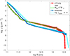Fig. A.1.

Density distributions for the modified progenitor structure (with outer layers cut, then stretched, and with an exponentially declining layer attached) versus radius, compared to the original s10 pre-collapse model. See text for details.

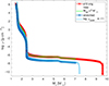Fig. A.2.

Density distribution for the modified progenitor structure (with outer layers cut, then stretched, and with an exponentially declining layer attached) versus mass coordinate, compared to the original s10 pre-collapse model. See text for details.

Appendix B: Appended circumstellar matter

For the models with CSM, we appended a wind-like layer to the constructed progenitor, what means that the density distribution in the CSM is ρ ∝ r⁻². The density at the inner boundary of the CSM spans a range of (0.3 − 118)×10^− 11 g cm^− 3 (see Table 2). Figure B.1 shows three models with the same CSM mass of 0.3 M_⊙ and three considered CSM radii, 1.5 × 10¹⁴ cm, 6 × 10¹⁴ cm, and 10¹⁵ cm standing for the W14, W2, and W7 models.

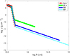Fig. B.1.

Density distribution for wind-models with the CSM mass of 0.3 M_⊙ for three considered CSM radii: 1.5 × 10¹⁴ cm (W14), 6 × 10¹⁴ cm (W2), and 10¹⁵ cm (W7).

Appendix C: Broadband light curves

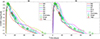Fig. C.1.

UVW2 magnitudes for models W1–W6, R_CSM = 6 × 10¹⁴ cm (a; left) and W7–W11, R_CSM = 10¹⁵ cm (b; right). The observational data are taken from Hiramatsu et al. (2023), Teja et al. (2023), and Singh et al. (2024).

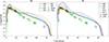Fig. C.2.

u magnitude for models W1–W6, R_CSM = 6 × 10¹⁴ cm (a; left) and W7–W11, R_CSM = 10¹⁵ cm (b; right). The observational data are taken from Teja et al. (2023) and Singh et al. (2024).

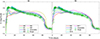Fig. C.3.

V magnitude for models W1–W6, R_CSM = 6 × 10¹⁴ cm (a; left) and W7–W11, R_CSM = 10¹⁵ cm (b; right). The observational data are taken from Hiramatsu et al. (2023) and Singh et al. (2024).

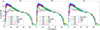Fig. C.4.

g magnitude for models W12–W17, R_CSM = 1.5 × 10¹⁴ cm (a; left); W1–W6, R_CSM = 6 × 10¹⁴ cm (b; middle); and W7–W11, R_CSM = 10¹⁵ cm (c; right). The observational data are taken from Hiramatsu et al. (2023), Teja et al. (2023), Li et al. (2024), and Singh et al. (2024).

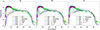Fig. C.5.

r magnitude for models W12–W17, R_CSM = 1.5 × 10¹⁴ cm (a; left); W1–W6, R_CSM = 6 × 10¹⁴ cm (b; middle); and W7–W11, R_CSM = 10¹⁵ cm (c; right). The observational data are taken from Hiramatsu et al. (2023), Teja et al. (2023), Li et al. (2024), and Singh et al. (2024).

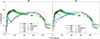Fig. C.6.

z magnitude for models W1–W6, R_CSM = 6 × 10¹⁴ cm (a; left) and W7–W11, R_CSM = 10¹⁵ cm (b; right). The observational data are taken from Hiramatsu et al. (2023), Teja et al. (2023), and Singh et al. (2024).

Appendix D: Earliest phase of the SN 2023ixf light curve

Here, we demonstrate that the best-fit wind-models, which were built to match the main SN 2023ixf LC over 100 days, overestimate the flux for the earliest epoch of the SN. In Fig. D.1, we show V-band LCs for the shell-models and wind-models W7, W10, and W11. Contrary to Fig. 3, the time interval is 15 days and the upper limit for magnitude is −19 mags (versus 16 hours and −13.5 mags). We note that the earliest data fall below the lower limit of Figs. 1, 2, and Fig. C.1–C.6. It is seen that the wind-models match the rising part of the SN 2023ixf LC, whereas these models have too high a flux during the first day after the discovery.

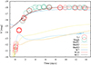Fig. D.1.

V-band LCs for our shell-models and the wind-models W7, W10, and W11. The observational data are taken from Li et al. (2024) (“Li”) and Singh et al. (2024) (“Singh”).

All Tables

Table 1.

Progenitor parameters of SN 2023ixf in the literature.

In the text

Table 2.

Supernova LC models presented in our study.

In the text

Table 3.

Shell model parameters.

In the text

All Figures

	Fig. 1. Bolometric LCs for a grid of models with CSM radii of 1.5 × 10¹⁴ cm (a; left), 6 × 10¹⁴ cm (b; middle), and 10¹⁵ cm (c; right). The observational data are taken from Bersten et al. (2024), Martinez et al. (2024), Singh et al. (2024), and Zimmerman et al. (2024).
In the text

	Fig. 2. Pseudo-bolometric LCs for a grid of models with CSM radii of 1.5 × 10¹⁴ cm (a; left), 6 × 10¹⁴ cm (b; middle), and 10¹⁵ cm (c; right). The observational data are taken from Hiramatsu et al. (2023), Hsu et al. (2024), and Singh et al. (2024).
In the text

Fig. 3.

Light curves of g, V, and r for a CSM model W17 with a compact CSM (1.5 × 10¹⁴ cm, 1.56 M_⊙), and shell models: ‘Shell1’, ‘Shell2’, and ‘Shell3’ with an inner radius of 700 R_⊙, outer radii of 1000 R_⊙, 900 R_⊙, and 800 R_⊙, masses of 0.9 M_⊙, 1 M_⊙, and 0.5 M_⊙, and injected energies of 0.01 foe, 0.02 foe, and 0.0185 foe, respectively. The observational data are taken from Li et al. (2024) and are shown by circles. The triangles indicate non-detection and are also from Li et al. (2024).

In the text

Fig. 4.

Axion parameter space. All shaded regions are excluded by one or more astrophysical probes. Specifically, the region above the blue line is excluded by the duration of the neutrino signal from SN 1987A (Raffelt 1996). The purple region is excluded by the explosion energies of Type IIP SNe (Caputo et al. 2022b), assuming a typical star with a radius of R_* = 5 × 10¹³ cm and a lower limit on the explosion energy of 0.1 foe. The grey region is constrained by measurements of the extragalactic background light (Caputo et al. 2022a), while the green region is excluded by the upper limit on the gamma-ray fluence from SN 1987A (Caputo et al. 2022a), as determined by GRS. The shaded orange region is instead in tension with X-ray observations of GW170817 event (Diamond et al. 2024). The red stars highlight points of the parameter space around which the axion’s mean free path is within ∼10¹² − 10¹⁴ cm and the energy deposition at such distances accrues to ∼0.01–0.1 foe.

In the text

	Fig. A.1. Density distributions for the modified progenitor structure (with outer layers cut, then stretched, and with an exponentially declining layer attached) versus radius, compared to the original s10 pre-collapse model. See text for details.
In the text

	Fig. A.2. Density distribution for the modified progenitor structure (with outer layers cut, then stretched, and with an exponentially declining layer attached) versus mass coordinate, compared to the original s10 pre-collapse model. See text for details.
In the text

	Fig. B.1. Density distribution for wind-models with the CSM mass of 0.3 M_⊙ for three considered CSM radii: 1.5 × 10¹⁴ cm (W14), 6 × 10¹⁴ cm (W2), and 10¹⁵ cm (W7).
In the text

	Fig. C.1. UVW2 magnitudes for models W1–W6, R_CSM = 6 × 10¹⁴ cm (a; left) and W7–W11, R_CSM = 10¹⁵ cm (b; right). The observational data are taken from Hiramatsu et al. (2023), Teja et al. (2023), and Singh et al. (2024).
In the text

	Fig. C.2. u magnitude for models W1–W6, R_CSM = 6 × 10¹⁴ cm (a; left) and W7–W11, R_CSM = 10¹⁵ cm (b; right). The observational data are taken from Teja et al. (2023) and Singh et al. (2024).
In the text

	Fig. C.3. V magnitude for models W1–W6, R_CSM = 6 × 10¹⁴ cm (a; left) and W7–W11, R_CSM = 10¹⁵ cm (b; right). The observational data are taken from Hiramatsu et al. (2023) and Singh et al. (2024).
In the text

	Fig. C.4. g magnitude for models W12–W17, R_CSM = 1.5 × 10¹⁴ cm (a; left); W1–W6, R_CSM = 6 × 10¹⁴ cm (b; middle); and W7–W11, R_CSM = 10¹⁵ cm (c; right). The observational data are taken from Hiramatsu et al. (2023), Teja et al. (2023), Li et al. (2024), and Singh et al. (2024).
In the text

	Fig. C.5. r magnitude for models W12–W17, R_CSM = 1.5 × 10¹⁴ cm (a; left); W1–W6, R_CSM = 6 × 10¹⁴ cm (b; middle); and W7–W11, R_CSM = 10¹⁵ cm (c; right). The observational data are taken from Hiramatsu et al. (2023), Teja et al. (2023), Li et al. (2024), and Singh et al. (2024).
In the text

	Fig. C.6. z magnitude for models W1–W6, R_CSM = 6 × 10¹⁴ cm (a; left) and W7–W11, R_CSM = 10¹⁵ cm (b; right). The observational data are taken from Hiramatsu et al. (2023), Teja et al. (2023), and Singh et al. (2024).
In the text

	Fig. D.1. V-band LCs for our shell-models and the wind-models W7, W10, and W11. The observational data are taken from Li et al. (2024) (“Li”) and Singh et al. (2024) (“Singh”).
In the text

Current usage metrics show cumulative count of Article Views (full-text article views including HTML views, PDF and ePub downloads, according to the available data) and Abstracts Views on Vision4Press platform.

Data correspond to usage on the plateform after 2015. The current usage metrics is available 48-96 hours after online publication and is updated daily on week days.

Initial download of the metrics may take a while.

[1] Ackermann, M., Ajello, M., Albert, A., et al. 2015, Astrophys. J., 799, 86 [CrossRef] [Google Scholar]

[2] Anderson, J. P., González-Gaitán, S., Hamuy, M., et al. 2014, ApJ, 786, 67 [Google Scholar]

[3] Ando, S., & Sato, K. 2004, New J. Phys., 6, 170 [NASA ADS] [CrossRef] [Google Scholar]

[4] Arnett, W. D. 1980, ApJ, 237, 541 [Google Scholar]

[5] Asplund, M., Grevesse, N., & Sauval, A. J. 2005, in Cosmic Abundances as Records of Stellar Evolution and Nucleosynthesis, eds. T. G. Barnes, III, & F. N. Bash, Astronomical Society of the Pacific Conference Series, 336, 25 [Google Scholar]

[6] Beacom, J. F. 2010, Ann. Rev. Nucl. Part. Sci., 60, 439 [NASA ADS] [CrossRef] [Google Scholar]

[7] Beasor, E. R., & Davies, B. 2018, MNRAS, 475, 55 [NASA ADS] [CrossRef] [Google Scholar]

[8] Bersten, M. C., Orellana, M., Folatelli, G., et al. 2024, A&A, 681, L18 [NASA ADS] [CrossRef] [EDP Sciences] [Google Scholar]

[9] Bianciardi, G., Ciccarelli, A. M., Conzo, G., et al. 2023, TNSAN, 213, 1 [NASA ADS] [Google Scholar]

[10] Bisnovatyi-Kogan, G. S., Popov, I. P., & Samokhin, A. A. 1976, Ap&SS, 41, 287 [NASA ADS] [CrossRef] [Google Scholar]

[11] Blinnikov, S. I., Eastman, R., Bartunov, O. S., Popolitov, V. A., & Woosley, S. E. 1998, ApJ, 496, 454 [Google Scholar]

[12] Blinnikov, S., Lundqvist, P., Bartunov, O., Nomoto, K., & Iwamoto, K. 2000, ApJ, 532, 1132 [NASA ADS] [CrossRef] [Google Scholar]

[13] Blinnikov, S. I., Röpke, F. K., Sorokina, E. I., et al. 2006, A&A, 453, 229 [NASA ADS] [CrossRef] [EDP Sciences] [Google Scholar]

[14] Blondin, S., Blinnikov, S., Callan, F. P., et al. 2022, A&A, 668, A163 [NASA ADS] [CrossRef] [EDP Sciences] [Google Scholar]

[15] Bollig, R., DeRocco, W., Graham, P. W., & Janka, H. T. 2020, Phys. Rev. Lett., 125, 051104; Erratum: Phys. Rev. Lett. 126, 189901 (2021) [NASA ADS] [CrossRef] [Google Scholar]

[16] Bollig, R., Yadav, N., Kresse, D., et al. 2021, ApJ, 915, 28 [NASA ADS] [CrossRef] [Google Scholar]

[17] Bostroem, K. A., Pearson, J., Shrestha, M., et al. 2023, ApJ, 956, L5 [NASA ADS] [CrossRef] [Google Scholar]

[18] Bostroem, K. A., Sand, D. J., Dessart, L., et al. 2024, ApJ, 973, L47 [NASA ADS] [CrossRef] [Google Scholar]

[19] Bugli, M., Guilet, J., & Obergaulinger, M. 2021, MNRAS, 507, 443 [NASA ADS] [CrossRef] [Google Scholar]

[20] Burrows, A. 2013, Rev. Mod. Phys., 85, 245 [Google Scholar]

[21] Burrows, A., & Vartanyan, D. 2021, Nature, 589, 29 [CrossRef] [PubMed] [Google Scholar]

[22] Burrows, A., Hayes, J., & Fryxell, B. A. 1995, ApJ, 450, 830 [NASA ADS] [CrossRef] [Google Scholar]

[23] Burrows, A., Wang, T., & Vartanyan, D. 2024, ApJ, 964, L16 [NASA ADS] [CrossRef] [Google Scholar]

[24] Caputo, A., & Raffelt, G. 2024, in 1st General Meeting and 1st Training School of the COST Action COSMIC WISPers, 1, 41 [NASA ADS] [Google Scholar]

[25] Caputo, A., Raffelt, G., & Vitagliano, E. 2022a, Phys. Rev. D, 105, 035022 [NASA ADS] [CrossRef] [Google Scholar]

[26] Caputo, A., Janka, H.-T., Raffelt, G., & Vitagliano, E. 2022b, Phys. Rev. Lett., 128, 221103 [CrossRef] [PubMed] [Google Scholar]

[27] Chandra, P., Chevalier, R. A., Maeda, K., Ray, A. K., & Nayana, A. J. 2024, ApJ, 963, L4 [NASA ADS] [CrossRef] [Google Scholar]

[28] Chevalier, R. A. 1976, ApJ, 207, 872 [NASA ADS] [CrossRef] [Google Scholar]

[29] Chiavassa, A. 2022, in The Origin of Outflows in Evolved Stars, eds. L. Decin, A. Zijlstra, & C. Gielen (Cambridge, UK: Cambridge University Press), IAU Symposium, 366, 101 [NASA ADS] [Google Scholar]

[30] Chiavassa, A., Plez, B., Josselin, E., & Freytag, B. 2009, A&A, 506, 1351 [NASA ADS] [CrossRef] [EDP Sciences] [Google Scholar]

[31] Cox, D. P. 1972, ApJ, 178, 169 [NASA ADS] [CrossRef] [Google Scholar]

[32] Dahlen, T., Strolger, L.-G., Riess, A. G., et al. 2004, ApJ, 613, 189 [NASA ADS] [CrossRef] [Google Scholar]

[33] Dessart, L., & Jacobson-Galán, W. V. 2023, A&A, 677, A105 [NASA ADS] [CrossRef] [EDP Sciences] [Google Scholar]

[34] Dessart, L., Hillier, D. J., Waldman, R., & Livne, E. 2013, MNRAS, 433, 1745 [NASA ADS] [CrossRef] [Google Scholar]

[35] Di Luzio, L., Giannotti, M., Nardi, E., & Visinelli, L. 2020, Phys. Rept., 870, 1 [NASA ADS] [Google Scholar]

[36] Diamond, M., Fiorillo, D. F. G., Marques-Tavares, G., & Vitagliano, E. 2023, Phys. Rev. D, 107, 103029; Erratum: Phys. Rev. D 108, 049902 [NASA ADS] [CrossRef] [Google Scholar]

[37] Diamond, M., Fiorillo, D. F. G., Marques-Tavares, G., Tamborra, I., & Vitagliano, E. 2024, Phys. Rev. Lett., 132, 101004 [NASA ADS] [CrossRef] [Google Scholar]

[38] Dong, Y., Sand, D. J., Valenti, S., et al. 2023, ApJ, 957, 28 [NASA ADS] [CrossRef] [Google Scholar]

[39] Ebinger, K., Curtis, S., Fröhlich, C., et al. 2019, ApJ, 870, 1 [NASA ADS] [Google Scholar]

[40] Ercolino, A., Jin, H., Langer, N., & Dessart, L. 2024, A&A, 685, A58 [NASA ADS] [CrossRef] [EDP Sciences] [Google Scholar]

[41] Ertl, T., Janka, H. T., Woosley, S. E., Sukhbold, T., & Ugliano, M. 2016, ApJ, 818, 124 [NASA ADS] [CrossRef] [Google Scholar]

[42] Falk, S. W., & Schramm, D. N. 1978, Phys. Lett. B, 79, 511 [NASA ADS] [CrossRef] [Google Scholar]

[43] Fang, Q., Moriya, T. J., Ferrari, L., et al. 2025, ApJ, 978, 36 [NASA ADS] [CrossRef] [Google Scholar]

[44] Ferrari, L., Folatelli, G., Ertini, K., Kuncarayakti, H., & Andrews, J. E. 2024, A&A, 687, L20 [NASA ADS] [CrossRef] [EDP Sciences] [Google Scholar]

[45] Flinner, N., Tucker, M. A., Beacom, J. F., & Shappee, B. J. 2023, Res. Notes Am. Astron. Soc., 7, 174 [NASA ADS] [Google Scholar]

[46] Fox, O. D., Van Dyk, S. D., Williams, B. F., et al. 2022, ApJ, 929, L15 [NASA ADS] [CrossRef] [Google Scholar]

[47] Fuller, J. 2017, MNRAS, 470, 1642 [NASA ADS] [CrossRef] [Google Scholar]

[48] Fuller, J., & Tsuna, D. 2024, Open J. Astrophys., 7, 47 [CrossRef] [Google Scholar]

[49] Gagliano, A., Berger, E., Villar, V. A., et al. 2025, ApJ, 978, 110 [NASA ADS] [CrossRef] [Google Scholar]

[50] Goldberg, J. A., Bildsten, L., & Paxton, B. 2019, ApJ, 879, 3 [Google Scholar]

[51] Goldberg, J. A., Jiang, Y.-F., & Bildsten, L. 2022a, ApJ, 929, 156 [NASA ADS] [CrossRef] [Google Scholar]

[52] Goldberg, J. A., Jiang, Y.-F., & Bildsten, L. 2022b, ApJ, 933, 164 [NASA ADS] [CrossRef] [Google Scholar]

[53] Grassberg, E. K., Imshennik, V. S., & Nadyozhin, D. K. 1971, Ap&SS, 10, 28 [Google Scholar]

[54] Grefenstette, B. W., Brightman, M., Earnshaw, H. P., Harrison, F. A., & Margutti, R. 2023, ApJ, 952, L3 [NASA ADS] [CrossRef] [Google Scholar]

[55] Hamuy, M. 2003, ApJ, 582, 905 [NASA ADS] [CrossRef] [Google Scholar]

[56] Heger, A., Jeannin, L., Langer, N., & Baraffe, I. 1997, A&A, 327, 224 [NASA ADS] [Google Scholar]

[57] Herant, M., Benz, W., Hix, W. R., Fryer, C. L., & Colgate, S. A. 1994, ApJ, 435, 339 [NASA ADS] [CrossRef] [Google Scholar]

[58] Hiramatsu, D., Tsuna, D., Berger, E., et al. 2023, ApJ, 955, L8 [NASA ADS] [CrossRef] [Google Scholar]

[59] Hirschi, R., Meynet, G., & Maeder, A. 2004, A&A, 425, 649 [NASA ADS] [CrossRef] [EDP Sciences] [Google Scholar]

[60] Hoof, S., & Schulz, L. 2023, JCAP, 03, 054 [CrossRef] [Google Scholar]

[61] Hosseinzadeh, G., Farah, J., Shrestha, M., et al. 2023, ApJ, 953, L16 [NASA ADS] [CrossRef] [Google Scholar]

[62] Hsu, B., Smith, N., Goldberg, J. A., et al. 2024, ApJ, submitted [arXiv:2408.07874] [Google Scholar]

[63] Itagaki, K. 2023, TNSTR, 2023-39, 1 [NASA ADS] [Google Scholar]

[64] Iwamoto, K., Mazzali, P. A., Nomoto, K., et al. 1998, Nature, 395, 672 [Google Scholar]

[65] Jacobson-Galán, W. V., Dessart, L., Jones, D. O., et al. 2022, ApJ, 924, 15 [CrossRef] [Google Scholar]

[66] Jacobson-Galán, W. V., Dessart, L., Margutti, R., et al. 2023, ApJ, 954, L42 [CrossRef] [Google Scholar]

[67] Jaeckel, J., Malta, P. C., & Redondo, J. 2018, Phys. Rev. D, 98, 055032 [CrossRef] [Google Scholar]

[68] Jäger, Z., Jr., Vinkó, J., Bíró, B. I., et al. 2020, MNRAS, 496, 3725 [CrossRef] [Google Scholar]

[69] Janka, H.-T. 2012, Annu. Rev. Nucl. Part. Sci., 62, 407 [NASA ADS] [CrossRef] [Google Scholar]

[70] Janka, H. T. 2017, in Handbook of Supernovae, eds. A. W. Alsabti, & P. Murdin (Cham: Springer), 1095 [CrossRef] [Google Scholar]

[71] Janka, H.-T., & Kresse, D. 2024, Ap&SS, 369, 80 [NASA ADS] [CrossRef] [Google Scholar]

[72] Janka, H. T., & Müller, E. 1996, A&A, 306, 167 [NASA ADS] [Google Scholar]

[73] Jerkstrand, A., Fransson, C., Maguire, K., et al. 2012, A&A, 546, A28 [NASA ADS] [CrossRef] [EDP Sciences] [Google Scholar]

[74] Kasen, D. 2006, ApJ, 649, 939 [NASA ADS] [CrossRef] [Google Scholar]

[75] Kasen, D., & Woosley, S. E. 2009, ApJ, 703, 2205 [NASA ADS] [CrossRef] [Google Scholar]

[76] Khabibullin, I. I., Churazov, E. M., Bykov, A. M., Chugai, N. N., & Sunyaev, R. A. 2023, MNRAS, 521, 5536 [NASA ADS] [CrossRef] [Google Scholar]

[77] Kilpatrick, C. D., Foley, R. J., Jacobson-Galán, W. V., et al. 2023, ApJ, 952, L23 [NASA ADS] [CrossRef] [Google Scholar]

[78] Kimura, S. S. 2024, arXiv e-prints [arXiv:2409.18935] [Google Scholar]

[79] Kippenhahn, R., & Meyer-Hofmeister, E. 1977, A&A, 54, 539 [NASA ADS] [Google Scholar]

[80] Klencki, J., Istrate, A., Nelemans, G., & Pols, O. 2022, A&A, 662, A56 [NASA ADS] [CrossRef] [EDP Sciences] [Google Scholar]

[81] Kozyreva, A., Blinnikov, S., Langer, N., & Yoon, S. C. 2014, A&A, 565, A70 [NASA ADS] [CrossRef] [EDP Sciences] [Google Scholar]

[82] Kozyreva, A., Nakar, E., & Waldman, R. 2019, MNRAS, 483, 1211 [NASA ADS] [CrossRef] [Google Scholar]

[83] Kozyreva, A., Nakar, E., Waldman, R., Blinnikov, S., & Baklanov, P. 2020a, MNRAS, 494, 3927 [NASA ADS] [CrossRef] [Google Scholar]

[84] Kozyreva, A., Shingles, L., Mironov, A., Baklanov, P., & Blinnikov, S. 2020b, MNRAS, 499, 4312 [NASA ADS] [CrossRef] [Google Scholar]

[85] Kozyreva, A., Janka, H.-T., Kresse, D., Taubenberger, S., & Baklanov, P. 2022, MNRAS, 514, 4173 [CrossRef] [Google Scholar]

[86] Kravchenko, K., Van Eck, S., Chiavassa, A., et al. 2018, A&A, 610, A29 [NASA ADS] [CrossRef] [EDP Sciences] [Google Scholar]

[87] Kresse, D., Ertl, T., & Janka, H.-T. 2021, ApJ, 909, 169 [NASA ADS] [CrossRef] [Google Scholar]

[88] Laplace, E., Justham, S., Renzo, M., et al. 2021, A&A, 656, A58 [NASA ADS] [CrossRef] [EDP Sciences] [Google Scholar]

[89] Lau, M. Y. M., Hirai, R., Mandel, I., & Tout, C. A. 2024, ApJ, 966, L7 [NASA ADS] [CrossRef] [Google Scholar]

[90] Li, G., Hu, M., Li, W., et al. 2024, Nature, 627, 754 [NASA ADS] [CrossRef] [Google Scholar]

[91] Lovegrove, E., Woosley, S. E., & Zhang, W. 2017, ApJ, 845, 103 [NASA ADS] [CrossRef] [Google Scholar]

[92] Mannucci, F., Della Valle, M., & Panagia, N. 2007, MNRAS, 377, 1229 [NASA ADS] [CrossRef] [Google Scholar]

[93] Manzari, C. A., Park, Y., Safdi, B. R., & Savoray, I. 2024, Phys. Rev. Lett., 133, 211002 [NASA ADS] [CrossRef] [Google Scholar]

[94] Mao, Y., Zhang, M., Cai, G., et al. 2023, TNSAN, 130, 1 [NASA ADS] [Google Scholar]

[95] Martinez, L., Bersten, M. C., Anderson, J. P., et al. 2022, A&A, 660, A41 [NASA ADS] [CrossRef] [EDP Sciences] [Google Scholar]

[96] Martinez, L., Bersten, M. C., Folatelli, G., Orellana, M., & Ertini, K. 2024, A&A, 683, A154 [NASA ADS] [CrossRef] [EDP Sciences] [Google Scholar]

[97] Matsumoto, T., & Metzger, B. D. 2022, ApJ, 936, 114 [CrossRef] [Google Scholar]

[98] Mazzali, P. A., Valenti, S., Della Valle, M., et al. 2008, Science, 321, 1185 [NASA ADS] [CrossRef] [Google Scholar]

[99] Meynet, G., Maeder, A., Schaller, G., Schaerer, D., & Charbonnel, C. 1994, A&AS, 103, 97 [Google Scholar]

[100] Mirizzi, A., Tamborra, I., Janka, H.-T., et al. 2016, Riv. Nuovo Cim., 39, 1 [NASA ADS] [Google Scholar]

[101] Moriya, T. J., & Singh, A. 2024, PASJ, 76, 1050 [NASA ADS] [CrossRef] [Google Scholar]

[102] Moriya, T. J., Subrayan, B. M., Milisavljevic, D., & Blinnikov, S. I. 2023, PASJ, 75, 634 [NASA ADS] [CrossRef] [Google Scholar]

[103] Müller, B. 2016, PASA, 33, e048 [Google Scholar]

[104] Müller, B., Heger, A., Liptai, D., & Cameron, J. B. 2016, MNRAS, 460, 742 [Google Scholar]

[105] Müller, B., Melson, T., Heger, A., & Janka, H.-T. 2017, MNRAS, 472, 491 [Google Scholar]

[106] Müller, E., Carenza, P., Eckner, C., & Goobar, A. 2024, Phys. Rev. D, 109, 023018 [CrossRef] [Google Scholar]

[107] Nakar, E., & Sari, R. 2010, ApJ, 725, 904 [NASA ADS] [CrossRef] [Google Scholar]

[108] Neustadt, J. M. M., Kochanek, C. S., & Smith, M. R. 2024, MNRAS, 527, 5366 [Google Scholar]

[109] Niu, Z., Sun, N.-C., Maund, J. R., et al. 2023, ApJ, 955, L15 [NASA ADS] [CrossRef] [Google Scholar]

[110] Obergaulinger, M., & Aloy, M. Á. 2021, MNRAS, 503, 4942 [NASA ADS] [CrossRef] [Google Scholar]

[111] O’Hare, C. A. J. 2024, PoS, COSMICWISPers, 040 [Google Scholar]

[112] Peccei, R. D., & Quinn, H. R. 1977, Phys. Rev. Lett., 38, 1440 [Google Scholar]

[113] Pejcha, O., & Prieto, J. L. 2015, ApJ, 806, 225 [Google Scholar]

[114] Pejcha, O., & Thompson, T. A. 2015, ApJ, 801, 90 [NASA ADS] [CrossRef] [Google Scholar]

[115] Pinto, P. A., & Eastman, R. G. 2000, ApJ, 530, 757 [NASA ADS] [CrossRef] [Google Scholar]

[116] Piran, T., Nakar, E., Mazzali, P., & Pian, E. 2019, ApJ, 871, L25 [NASA ADS] [CrossRef] [Google Scholar]

[117] Pledger, J. L., & Shara, M. M. 2023, ApJ, 953, L14 [NASA ADS] [CrossRef] [Google Scholar]

[118] Popov, D. V. 1993, ApJ, 414, 712 [NASA ADS] [CrossRef] [Google Scholar]

[119] Powell, J., Müller, B., Aguilera-Dena, D. R., & Langer, N. 2023, MNRAS, 522, 6070 [NASA ADS] [CrossRef] [Google Scholar]

[120] Qin, Y.-J., Zhang, K., Bloom, J., et al. 2024, MNRAS, 534, 271 [NASA ADS] [CrossRef] [Google Scholar]

[121] Quataert, E., & Shiode, J. 2012, MNRAS, 423, L92 [NASA ADS] [CrossRef] [Google Scholar]

[122] Quataert, E., Fernández, R., Kasen, D., Klion, H., & Paxton, B. 2016, MNRAS, 458, 1214 [NASA ADS] [CrossRef] [Google Scholar]

[123] Raffelt, G. G. 1996, Stars as laboratories for fundamental physics: The astrophysics of neutrinos, axions, and other weakly interacting particles (Chicago : University of Chicago Press) [Google Scholar]

[124] Ransome, C. L., Villar, V. A., Tartaglia, A., et al. 2024, ApJ, 965, 93 [CrossRef] [Google Scholar]

[125] Safdi, B. R. 2024, PoS, TASI2022, 009 [Google Scholar]

[126] Sgro, L. A., Esposito, T. M., Blaclard, G., et al. 2023, Res. Notes Am. Astron. Soc., 7, 141 [Google Scholar]

[127] Shivvers, I., Modjaz, M., Zheng, W., et al. 2017, PASP, 129, 054201 [NASA ADS] [CrossRef] [Google Scholar]

[128] Shrestha, M., Bostroem, K. A., Sand, D. J., et al. 2024, ApJ, 972, L15 [Google Scholar]

[129] Shussman, T., Waldman, R., & Nakar, E. 2016, arXiv e-prints [arXiv:1610.05323] [Google Scholar]

[130] Singh, A. P., Richards, A. M. S., Humphreys, R. M., Decin, L., & Ziurys, L. M. 2023, ApJ, 954, L1 [NASA ADS] [CrossRef] [Google Scholar]

[131] Singh, A., Teja, R. S., Moriya, T. J., et al. 2024, ApJ, 975, 132 [CrossRef] [Google Scholar]

[132] Soker, N. 2024, Open J. Astrophys., 7, 69 [Google Scholar]

[133] Soraisam, M. D., Szalai, T., Van Dyk, S. D., et al. 2023, ApJ, 957, 64 [NASA ADS] [CrossRef] [Google Scholar]

[134] Spiro, S., Pastorello, A., Pumo, M. L., et al. 2014, MNRAS, 439, 2873 [Google Scholar]

[135] Stockinger, G., Janka, H. T., Kresse, D., et al. 2020, MNRAS, 496, 2039 [Google Scholar]

[136] Strotjohann, N. L., Ofek, E. O., Gal-Yam, A., et al. 2021, ApJ, 907, 99 [NASA ADS] [CrossRef] [Google Scholar]

[137] Sukhbold, T., Ertl, T., Woosley, S. E., Brown, J. M., & Janka, H. T. 2016, ApJ, 821, 38 [NASA ADS] [CrossRef] [Google Scholar]

[138] Teja, R. S., Singh, A., Basu, J., et al. 2023, ApJ, 954, L12 [NASA ADS] [CrossRef] [Google Scholar]

[139] Tinyanont, S., Ridden-Harper, R., Foley, R. J., et al. 2022, MNRAS, 512, 2777 [NASA ADS] [CrossRef] [Google Scholar]

[140] Tsuna, D., Huang, X., Fuller, J., & Piro, A. L. 2024, ApJ, accepted [arXiv:2410.07055] [Google Scholar]

[141] Turner, M. S. 1988, Phys. Rev. Lett., 60, 1797 [NASA ADS] [CrossRef] [Google Scholar]

[142] Ugliano, M., Janka, H.-T., Marek, A., & Arcones, A. 2012, ApJ, 757, 69 [NASA ADS] [CrossRef] [Google Scholar]

[143] Van Dyk, S. D., Srinivasan, S., Andrews, J. E., et al. 2024, ApJ, 968, 27 [NASA ADS] [CrossRef] [Google Scholar]

[144] Vasylyev, S. S., Yang, Y., Filippenko, A. V., et al. 2023, ApJ, 955, L37 [NASA ADS] [CrossRef] [Google Scholar]

[145] Weiler, K. W., van Dyk, S. D., Pringle, J. E., & Panagia, N. 1992, ApJ, 399, 672 [NASA ADS] [CrossRef] [Google Scholar]

[146] Weinberg, S. 1978, Phys. Rev. Lett., 40, 223 [Google Scholar]

[147] Wilczek, F. 1978, Phys. Rev. Lett., 40, 279 [Google Scholar]

[148] Wood, P. R., Bessell, M. S., & Fox, M. W. 1983, ApJ, 272, 99 [Google Scholar]

[149] Woosley, S. E. 1988, Astrophys. J., 330, 218 [NASA ADS] [CrossRef] [Google Scholar]

[150] Wu, S., & Fuller, J. 2021, ApJ, 906, 3 [NASA ADS] [CrossRef] [Google Scholar]

[151] Xiang, D., Mo, J., Wang, L., et al. 2024, Sci. China: Phys. Mech. Astron., 67, 219514 [NASA ADS] [CrossRef] [Google Scholar]

[152] Yoon, S.-C., & Cantiello, M. 2010, ApJ, 717, L62 [NASA ADS] [CrossRef] [Google Scholar]

[153] Yoon, S. C., Gräfener, G., Vink, J. S., Kozyreva, A., & Izzard, R. G. 2012, A&A, 544, L11 [NASA ADS] [CrossRef] [EDP Sciences] [Google Scholar]

[154] Zel’dovich, Y. B., & Raizer, Y. P. 1967, Physics of shock waves and high-temperature hydrodynamic phenomena (New York: Academic Press) [Google Scholar]

[155] Zhang, J., Lin, H., Wang, X., et al. 2023, Sci. Bull., 68, 2548 [NASA ADS] [CrossRef] [Google Scholar]

[156] Zimmerman, E. A., Irani, I., Chen, P., et al. 2024, Nature, 627, 759 [Google Scholar]