| Issue |
A&A
Volume 695, March 2025
|
|
|---|---|---|
| Article Number | A267 | |
| Number of page(s) | 10 | |
| Section | Stellar structure and evolution | |
| DOI | https://doi.org/10.1051/0004-6361/202348689 | |
| Published online | 26 March 2025 | |
Can circumstellar interaction explain the strange light-curve features of Type Ib/c supernovae?
1
Department of Experimental Physics, Institute of Physics, University of Szeged, Dóm tér 9, 6720 Szeged, Hungary
2
ELKH-SZTE Stellar Astrophysics Research Group, Szegedi út, Kt. 766, 6500 Baja, Hungary
⋆ Corresponding author; This email address is being protected from spambots. You need JavaScript enabled to view it.
Received:
21
November
2023
Accepted:
24
January
2025
Abstract
Context. The evolution and surrounding of the progenitors of stripped-envelope supernovae are still debated: some studies suggest single-star progenitors, but others prefer massive binary progenitors. Moreover, the basic physical properties of the exploding star and its interaction with circumstellar matter could significantly modify the overall light-curve features of these objects. To better understand the effect of stellar evolution and circumstellar interaction, systematic hydrodynamic calculations are needed.
Aims. We test the hypothesis that circumstellar matter generated by an extreme episodic η Carinae-like eruption that occurs days or weeks before the supernova explosion may explain the differences related to the general light-curve features of stripped-envelope supernovae.
Methods. We present our bolometric light-curve calculations of single-star and binary progenitors generated by hydrodynamic simulations via MESA and SNEC. We also studied the effect of an interaction with close low-mass circumstellar matter assumed to be created just a few days or weeks before the explosion. In addition to generating a model light-curve grid, we compared our results with some observational data.
Results. We found that the shape of the supernova light curve alone can indicate that the cataclysmic death of the massive star occurred in a binary system or was related to the explosion of a single star. Moreover, our study also shows that confined dense circumstellar matter may cause the strange light-curve features (bumps, rebrightening, or steeper tail) of some Type Ib/c supernovae.
Key words: hydrodynamics / circumstellar matter / stars: evolution / supernovae: general
© The Authors 2025
 Open Access article, published by EDP Sciences, under the terms of the Creative Commons Attribution License (https://creativecommons.org/licenses/by/4.0), which permits unrestricted use, distribution, and reproduction in any medium, provided the original work is properly cited.
This article is published in open access under the Subscribe to Open model. This email address is being protected from spambots. You need JavaScript enabled to view it. to support open access publication.
1. Introduction
Core-collapse supernovae (SNe) are formed from the gravitational collapse of the nickel-iron core of massive stars. Although the explosion mechanism is the same, these transients can be extremely different from an observational point of view: We can distinguish H-rich (Type IIP or IIL), H-poor (Type IIb), and H-free (Type Ib/c) explosions. The group of Type IIb together with Type Ib/c is also called stripped-envelope supernovae (SESNe). The noticeable differences in the spectral and light-curve (LC) features mainly depend on the mass-loss history of the progenitor star (e.g. Limongi 2017; Vink 2022).
The light curves of SESNe are mainly powered by the radioactive decay of nickel and cobalt as well as gamma-ray (e.g. Arnett & Fu 1989; Clocchiatti & Wheeler 1997). The estimated nickel mass of these explosions is about 0.03–0.35 M⊙ (Taddia et al. 2018). According to analytic and hydrodynamic calculations, their progenitors are quite compact (Rp ∼ 109 − 1010 cm), and the early luminosity of these events mainly depends on the progenitor radius. The ejected masses during the explosion are relatively low (Mej ∼ 1.1 − 10.1 M⊙), while the explosion energy of these objects is about 0.25 − 4.9 ⋅ 1051 erg (e.g. Lyman et al. 2016; Taddia et al. 2018). In some cases, an initial peak can be detected, followed by a rapid drop in luminosity. This early emission is thought to be driven by the shock breakout or an extended envelope around the progenitor (e.g. Bersten et al. 2013; Nagy & Vinkó 2016).
The explosion may occur within circumstellar matter (CSM) that formed throughout the stellar evolution, even though some supernova subtypes (IIn, Ibn, and Icn) show significant CSM interaction features in their spectra and luminosities (Fraser 2020; Dessart et al. 2022; Maeda & Moriya 2022; Takei et al. 2024). The circumstellar matter could play an important role in generating the light curve of some superluminous SNe even when there are no obvious spectral signs of the interaction (Moriya & Maeda 2012; Mazzali et al. 2016; Wheeler et al. 2017). Moreover, as Kuncarayakti et al. (2022) revealed, normal Type Ic supernovae may show similar spectroscopic features to interacting Type Ibn and Icn SNe in late phases. These phenomena, and the fact that we do not know exactly when massive stars, especially stripped-envelope supernova (SESN) progenitors, lost their outer hydrogen and/or helium layers, suggest a possible circumstellar interaction for Type Ib/c supernovae as well.
As far as we know, SESN progenitors experience significant mass loss during the pre-supernova evolution, but the exact mechanism is still debated. Some observations suggest (e.g. Cao et al. 2013) a massive single-star (possibly a Wolf-Rayet star) progenitor that loses its outer envelope due to an extreme stellar wind or irregular eruption phases. However, other studies (e.g. Sana et al. 2012; Woosley et al. 2021) assumed binary interaction before the explosion that strips the outermost layers of the massive donor star. The commonality in the two scenarios is that they suggest circumstellar matter around the progenitor star.
Even though recent studies reported a possible connection between CSM interaction and the re-brightening of late-time (200 ≲ days after the explosion) SESNe light curves (Sollerman et al. 2020; Soraisam et al. 2022; Kuncarayakti et al. 2023), these results indicate a circumstellar ring with a very thin inner edge around 5 ⋅ 1015 − 1016 cm. On the other hand, theoretical considerations (Benetti et al. 2018; Maeda et al. 2021, e.g.) suggested that the CSM radius around a stripped-envelope supernova progenitor should be 1014 − 1015 cm, which presumes that this matter is ejected just a few months before the SN explosion. This controversy may be resolved when we assume an extreme episodic mass-loss event (0.1–1 M⊙) at the end of the stellar evolution, caused by somewhat similar physical processes as were observed in the case of η Carinae (Vamvatira-Nakou et al. 2016). This theory may also explain the earlier (around 60–100 days after the explosion) light curve bumps of SESNe if an eruption occurs days or weeks before the supernova explosion. An event like this is more than plausible because precursor outbursts shortly before the explosion have been observed in some cases. For example, an optical transient in 2004 can be connected to the Type Ic explosion SN 2006jc (Pastorello et al. 2007), while according to Ho et al. (2019), the progenitor of SN 2018gep also produced outbursts just days to months before the explosion. Moreover, observational data also suggest that precursor outbursts could be common but less energetic and be shorter for types other than IIn (Strotjohann et al. 2021).
In addition to an intense eruption (Mcley & Soker 2014), when the primary and the secondary components in binary systems have a strong stellar wind, a colliding-wind structure (CWS) (e.g. Kashi & Michaelis 2021, and reference within) can be formed. This dense formation may mimic a close CSM around the star as supernova ejecta interacts with it, as suggested by Kochanek (2019) for the H-poor (Type IIb) stripped-envelope supernova iPTF13as (SN 2013cu). In these cases, the additional luminosity excess is due to an additional power source related to the interaction between the SN ejecta and a close CSM (e.g. Chevalier & Fransson 2006), as the mass-loss history shortly before the SN explosion can drastically influence the optical light curve properties (e.g., brightness and color) of Type Ib/c progenitors (Jung et al. 2022).
Accordingly, numerical studies might be crucial for revealing the nature of this early CSM interaction and expose a possible mass-loss episode shortly before the supernova explosion. To do this, we started our work by adding an attached relatively thin CSM layer much closer than in previous works that modeled type Ibn/Icn explosions (e.g. Kuriyama & Shigeyama 2020; Maeda & Moriya 2022; Takei et al. 2024). The radius of our CSM models was defined by multiplying the radius of the progenitor models with factors from 2 to 10. Because our model progenitor stars are compact, the radius of the attached CSM in this way does not exceed 10 R⊙ in any case. We applied one-dimensional hydrodynamic calculations to generate the bolometric light curves from SESN progenitor models that interact with close low-mass (MCSM ≤ 2 M⊙) circumstellar matter. We introduce our systematic studies of the effect of the radius and mass of the CSM, as well as the different physical compositions of the progenitors.
This paper is organized as follows: We present our model setups and numerical method in Sect. 2. We discuss the most important properties of our synthetic light curves in Sect. 3. We compare our result with some well-known SESNe in Sect. 4. Finally, we provide a summary of our conclusion in Sect. 5.
2. Model setups
We performed complete hydrodynamical modeling and analytic approximations to create a unique physical configuration that is self-consistent with a supernova explosion in close circumstellar matter caused by an extreme mass-loss event just a few days or weeks before the cataclysm.
We calculated single-star and binary progenitor models using the code Modules for Experiments in Stellar Astrophysics (MESA version r-12778), which is a one-dimensional numerical hydrodynamic stellar evolution code (Paxton et al. 2011, 2013, 2015, 2018, 2019; Jermyn et al. 2023). Then, we generated different thin (RCSM ≤ 10 Rp) low-mass (MCSM ≤ 2 M⊙) CSM configurations with a power-law density profile using an analytical code and added them to the MESA models. As a final step, we calculated the bolometric light curves of our progenitor models with and without the attached circumstellar matter using the one-dimensional spherical Lagrangian SuperNova Explosion Code (SNEC, Morozova et al. 2015).
2.1. Progenitor models
A detailed explanation of the progenitor models is beyond the scope of this paper (more specifications are provided in our forthcoming paper). We describe the basic simulation setup for numerically generating a proper environment for our assumed CSM-interacting SESNe to test the effect of a close low-mass circumstellar matter.
2.1.1. Single-star models
First, we created stellar models for single massive stars to create Type Ibc SN progenitors. Our calculations ran from the zero-age main sequence (ZAMS) to the end of the helium burning. Then, we adopted a manually adjusted mass_change parameter with a value of 10−2 M⊙/yr to remove the remaining hydrogen (and helium) layers before Fe-core collapse. This average mass-loss rate was at about the same order of magnitude as was calculated for the great 1840 eruption of η Carinae (Andriesse & Viotti 1979). From a modeling point of view, this more extreme mass-loss phase could correspond to an intensive late-time outburst. This is self-consistent with our CSM-forming premise.
We took stellar evolution models with initial masses of 15, 20, and 50 M⊙, which correspond to the estimated mass range of SESN progenitors (Georgy et al. 2009). In all 14 models, we assumed semi-convection (alpha_semiconvection =0.01), overshooting with f0 = 0.0005, and mixing (mixing_length_alpha =1.5), and we set the varcontrol_target =10−3 for the convergence of models with higher mass-loss. To avoid numerical problems and to speed up our calculations, we changed the nuclear reaction rate network from ‘basic.net’ to ‘approx21.net’ with the Heger-style adaptive network option (Woosley et al. 2004). We also used the Ledoux convection criterion to determine the position of the non-radiative boundaries within our stellar model.
In our model grid, we systematically studied some modeling parameters (related to metallicity, stellar wind type, and its scaling factor) that can alter the physical properties and mass loss of the progenitor. For each mass, the reference parameters were Z = 0.02, so-called Dutch stellar wind schemes (Glebbeek et al. 2009; Nugis & Lamers 2000) for the asymptotic giant branch phase, and ηdutch = 0.8 for the wind scaling factor. Then, we varied these parameters one by one to examine their effect. Some properties of the progenitors are provided in Table 1. The table lists details of the initial (M) and final masses, the radius of the progenitors (MIbc and Rp), their He-mass (MHe) after the assumed intensive mass-loss phase that creates Type Ibc explosions, the total mass loss (dM) caused by stellar wind, and the mass_change parameter.
Physical properties of our single-star models.
2.1.2. Binary star models
We mainly focused on close binary systems (initial rotational period Pinit < 100 days), where we considered the primary and secondary components as massive stars. We also assumed that higher initial mass (Minit) belonged to the donor star, which evolves to an SESN progenitor due to mass loss. In our total of 16 models, we varied the initial mass of the donor within 35–60 M⊙ while altering Minit for the secondary component to 12–42 M⊙. We also used different metallicities (Z), initial rotational periods, and mass ratios (q) to describe the binary system. We also determined the total mass-loss for the donor (dM) and the mass of its remaining He layer (MHe) at the time of the core collapse (Table 2). All models showed some amount of He, but according to the synthetic spectral studies of Hachinger et al. (2012), some might form He-free spectra because approximately 0.06–0.14 M⊙ of helium can be hidden and lead to a classification as Type Ic. Thus, we can classify our binary models as possible Type Ib/c progenitors with a final mass of MIbc, as also listed in Table 2.
Physical properties of our binary star models.
We also selected the parameter space of our binary models so that they could be initialized as circular systems by MESA because in this case, the code can monitor the changes in the orbital angular momentum (Jorb) during binary evolution. This is essential because heavy mass transfer, among others (gravitational waves, magnetic braking, and spin-orbit coupling) strongly affects the orbit of the binary system. With this approximation, we were able to create self-consistent binary models that took the alterations of Jorb into account (see Eq. (3). in Paxton et al. 2015).
We considered a fully non-conservative mass transfer for our binary models that can be represented in MESA with a zero mass_transfer_gamma and mass_transfer_delta value. At the same time, we fixed the mass_transfer_alpha and mass_transfer_beta parameters to 0.5 (Petrovic et al. 2005; Shao & Li 2016).
All simulations started from the zero-age main sequence and followed the evolution of the binary system until the donor evolved to near the core-collapse phase. Nevertheless, none of them reached this state for numerical reasons. However, most of the Ne was created in the center (except for models 9 and 10) or even formed a Si core, which is only years to days before the formation of the iron core. In addition to reaching core-collapse in a binary, we aimed to generate potential progenitor models for stripped-envelope supernovae. Thus, our models needed to lose their entire H and even a good portion of their He layers, and their final mass should agree well with previous studies suggesting ejecta with 2–10 M⊙ (e.g. Jin et al. 2023, and reference within). In addition to Roche-lobe overflow, we initialized our MESA models with stellar winds using the Dutch hot-wind-scheme option with a scaling factor ηDutch = 1.0 to do this, and we switched the super-Eddington wind on in later evolutionary phases. When some additional energy (via unstable fusion, wave heating, or a binary companion) heats the near-surface region of the star, the stellar photosphere may exceed the Eddington luminosity, resulting in mass loss (Quataert et al. 2016). This is called super-Eddington wind, and it can surpass the effect of the metallicity-driven stellar wind. Note that from a modeling point of view, super-Eddington wind setups in MESA can control additional mass-loss, like the mass_change parameter does for the single-star models. However, the super-Eddington wind configuration describes a realistic physical phenomenon, while the mass_change parameter indicates a fixed, arbitrary mass loss. To create a self-consistent physical configuration for our binary models, we implemented the super-Eddington wind scheme in our simulations. We also implemented the default values for control parameters: super_eddington_wind_Ledd_factor = 1 and super_eddington_scaling_factor = 1. In this manner, we followed the classic theoretical condition. Namely, mass loss starts when the effective surface luminosity surpasses the Eddington luminosity.
However, as shown, for instance, by Pauli et al. (2023), the mass transfer to a close companion star should be the real engine of the heavy mass loss. Previous studies also suggested that Wolf-Rayet stars in binary systems tend to occur in low-metallicity environments. Thus, the effect of the metallicity-driven wind is thought to be negligible compared to the mass transfer between the two components. Considering these statements, we mainly focused on low-metallicity models in our study.
In MESA, two different approaches are available for modeling the acceptor star. We can assume that a secondary component remains a steady mass point. Alternatively, this object can evolve in time, like the donor star. We tested both scenarios and found no significant difference in the physical properties of the primary component. The main reason for this might be that regardless of Minit, 2, the direction of the mass transfer does not change during the simulation, and the acceptor remains in the same evolutionary stage. Thus, the secondary component has no direct impact on the inner structure of the donor star.
2.2. CSM properties
In the literature, some complex density profiles are available for modeling the structure of the circumstellar matter. One possibility is the double power-law density profile by Tsuna & Takei (2023), which describes the transition from the bound to the unbound parts of the close CSM that is attached to the progenitor star. However, this scenario only explains the CSM generated by the eruptions of a single star. Thus, to ensure that the single-star and binary models were comparable, we used a simplified CSM structure to examine the effect of a close, dense material cloud around the exploding stars. We assumed that the circumstellar matter was attached to the progenitor. Thus, the inner radius of it is equal to the radius of the progenitor. We adopted a power-law density profile, where the initial density of the CSM (ρ0) was estimated to be identical to the density at the progenitor surface (Fig. 1) and its value proportionate to the quadratic of the radius element of the CSM (r) as
 (1)
(1)
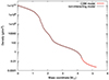 |
Fig. 1. Comparison of the initial density profile of a non-interacting and an interacting single-star model. The black line represents the non-interacting reference model, and the red line shows the total density profile of the same model with an added CSM profile. |
We also assumed that the mass of the CSM was independent of the CSM radius, as they are both grid parameters of the numerical simulation (Tsuna & Takei 2023). This indicates that the MCSM parameter cannot be derived from the average mass-loss rate and wind velocity (Chevalier & Fransson 2003), but is just an arbitrary model parameter. We still estimated an average wind velocity of 2000 km/s as the velocity of our CSM configuration.
The chemical composition of the circumstellar matter was assumed to be solar-like, mainly containing hydrogen and helium. A pure He composition would be more realistic as the expected blown-off layer of a massive, convective star in this late evolution phase. However, SNEC calculations become extremely time-consuming, and in many cases, numerically unstable for an H-free CSM. Moreover, no significant differences can detected for the overall light curve features or maximum luminosities, except that the first peak shows a steeper luminosity cut (Fig. 2). Because we are only interested in the general LC characteristics, we therefore chose to apply a solar-like chemical composition to our CSM structures.
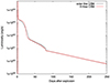 |
Fig. 2. Comparison of the calculated bolometric light curves for interacting CSM models (MCSM = 2 M⊙, RCSM = 10 Rp ) with different abundances. The red curve represents the H-free CSM, and the black line shows a solar-like chemical composition. |
The radius of the confined CSM was constrained to be smaller than ten times the progenitor radius, and MCSM was 2 M⊙ at most. In our model grid, we adopted RCSM of 2, 5, and 10 Rp, and a CSM mass of 0.01, 0.05, 0.1, 0.5, 1, and 2 M⊙ as an addition for all progenitor models. For the single-star models, these assumptions correspond well with the last-stage mass-loss history (controlled by mass_change parameter) of the progenitor stars. On the other hand, we lack modeling evidence for the mass-loss history of our binary configurations, as none of them reached the core-collapse phase. From a theoretical point of view, it therefore seemed reasonable to assume a similar CSM structure for binaries and single-star models.
2.3. Explosion properties
Because it is a radiation hydrodynamic code, SNEC (Morozova et al. 2015) can take the interaction between SN ejecta and CSM into account in computing bolometric light curves, which is needed to compare our results with observational data, whose bolometric LCs contain unexpected luminosity variations (bumps or a rebrightening). To test the effect of a CSM interaction, we simulated the explosion of all the previously described progenitor models with and without a mounted CSM shell.
We adopted a fixed excited mass (Mex = 1.4 M⊙ suggested by Morozova et al. 2015), explosion energy (Eexp = 1.5 ⋅ 1051 erg), and nickel masses (MNi = 0.1 M⊙) to reduce the strong impact of these parameters that can alter our results. Unfortunately, the effect of nickel cannot be eliminated because SNEC sums this implemented nickel mass value with the nickel content of the initial interacting or non-interacting stellar model, which is approximately 10−8 − 10−9 M⊙ and 0.025 − 0.03 M⊙ for binary and single-star models, respectively. Moreover, not just the nickel content, but the distribution of 56Ni and the overall density profile of our stellar models can also affect the obtained light curves. When we fixed the MNi parameter, the tail of the light curve therefore still depended on the initial nickel mass that was generated via stellar evolution. We therefore adopted an MNi value that corresponded well with observations and theoretical models. Previous observations suggested that the typical nickel mass for SESNe should be about 0.05 − 0.5 M⊙ (Lyman et al. 2016; Taddia et al. 2015), while recent studies indicated a range of 0.06 − 0.132 M⊙ (Rodríguez et al. 2023). From a theoretical point of view, the expected nickel mass for these objects is about 0.01 − 0.1 M⊙ (Müller et al. 2017; Ouchi et al. 2021; Dessart et al. 2022). Our selected MNi value could be reasonable for both observational and theoretical aspects. The chosen Eexp value is within the typical explosion energy range of Type Ib/c supernovae obtained from analytic and hydrodynamic calculations. To define the same explosion energy, we therefore set the ‘Bomb_mode’ option accordingly. As a default, SNEC determines the explosion energy as the total energy of the supernova environment. Thus, the code subtracts the binding energy of the exploding star (Ebin < 0) from the inserted thermal bomb energy (ESN). The actual explosion energy therefore is Eexp = ESN − Ebin, which can differ from one model to the next as it corresponds to the asymptotic energy of the system (SNEC users manual1). However, when we use the non-default ‘Bomb_mode =2’ option, the explosion energy is assumed to be equal to the specified thermal bomb energy parameter (Eexp = ESN). For better understanding, the difference between the obtained bolometric light curves using the two optional ‘Bomb_mode’ options are shown in Fig. 3. For a more self-consistent comparison, the non-default (‘Bomb_mode =2’) setting could be a reasonable choice because it allows us to fix the explosion energies. In the further calculations, we therefore used this option.
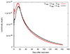 |
Fig. 3. Comparison of calculated bolometric light curves with different ‘Bomb_mode’ options. The red curve represents ‘Bomb_mode =1’, where Eexp = ESN − Ebin, and the black lines show the fixed explosion energy option (‘Bomb_mode =2’). |
Note that the solver controls, opacity option, and equation of state (EOS) were set as defaults during our calculations. SNEC calculates the opacity of each grid point from Rosseland mean opacity tables that consider the chemical composition, temperature, and density of matter. In addition, it requires the so-called opacity floor parameters that are by default 0.01 and 0.24 for the envelope (Z < 1) and the core (Z = 1), respectively. These specific opacity floor values are based on the calculations by Bersten et al. (2011) and provide a calibration between LTE and multi-frequency codes. On the other hand, in SNEC, the equation of state calculations adopt simplified analytic functions. By default, these equations are based on the study of Paczynski (1983), which determined the EOS for a mixture of ions, photons, and semi-relativistic electrons.
3. Bolometric light curves
The bolometric light curves of all non-interacting progenitor models show some general features of Type Ib/c supernova explosions. However, those that were generated from binary models typically produce fainter light curves with broader peaks than single-star light curves with about the same progenitor mass, explosion energies, and nickel masses (see Fig. 4). This phenomenon may occur due to the different compactness and initial nickel masses of single-star and binary progenitors with similar masses. When we compare the Rp values for single-star and binary models (Tables 1–2) within the same mass range, the single-star progenitor is about two to three times more extended than the binary progenitor. Moreover, as we fixed the additional nickel mass generated by the supernova explosion, Fig. 4 suggests that the initial nickel content of the binary progenitor models is much lower than that of single-star progenitors with similar masses.
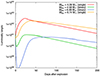 |
Fig. 4. Comparison of single-star and binary models with a similar progenitor mass. The red and orange lines represent single-star models with 4.28 and 6.74 M⊙, and green and blue lines show binary calculations with 4.58 and 6.68 M⊙, respectively. |
Note that we can generate similar peak luminosities for the single-star and binary models when we explode binary progenitors with higher energies and nickel masses. For example, the MIbc = 4.58 M⊙ binary model needed 3 ⋅ 1051 erg and 0.25 M⊙ to create a similar light curve maximum as the MIbc = 4.28 M⊙ single-star model with our fixed values of energy (1.5 ⋅ 1051) and nickel mass (0.1 M⊙). Nevertheless, the global LC features show some differences (Fig. 5): The peak is broader for the binary models, for example.
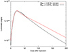 |
Fig. 5. Comparison of a single-star and a binary progenitor model calculated with MIbc and similar peak luminosities. |
In the further calculations, we used these non-interacting models as references and examined the effect of the interaction between the supernova ejecta and a thin, low-mass CSM shell. As all simulations showed the same characteristic features, we demonstrate our results via a one-on-one particular model related to single- and binary progenitors with a 4.28 M⊙ (Table 1, S1) and 4.58 M⊙ (Table 2, B12) final mass, respectively.
First, we examined the effect of the CSM mass on the bolometric light curve while its radius was fixed at 10 ⋅ Rp. Figures 6 and 7 show our results for interacting single and binary stars, respectively. Some general features can be seen in the generated LCs of both progenitor scenarios, such as the appearance of a fast-declining early part similar to the first peak in Type IIb and IIP supernova light curves, which is also associated with a low-mass CSM envelope (Chugai et al. 2007; Moriya et al. 2011; Nagy & Vinkó 2016). With increasing MCSM, this early LC characteristic becomes less luminous and broader, while the main light curve peak also changes significantly by the early bump. Moreover, with higher CSM mass, the late-time light curves depart progressively from the nickel-cobalt tail, and its slope becomes less steep.
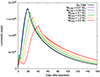 |
Fig. 6. Effect of a different CSM mass on the bolometric light curves of single-star models. The black line represents the non-interacting reference model (Table 1, S1). In contrast, the violet, dark blue, light blue, green, orange, and red lines illustrate the effect of circumstellar matter with a mass of 0.01, 0.05, 0.1, 0.5, 1, and 2 M⊙, respectively. |
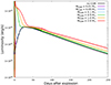 |
Fig. 7. Effect of a different CSM mass on the bolometric light curves of binary models. The black line represents the non-interacting reference model (Table 2, B12). In contrast, the violet, dark blue, light blue, green, orange, and red lines illustrate the effect of circumstellar matter with a mass of 0.01, 0.05, 0.1, 0.5, 1, and 2 M⊙, respectively. |
On the other hand, the alteration of the second peak shows different attributes in the case of single-star and binary models. The interacting binary models preserve their rise time to the main maximum and remain about the same, regardless of the interaction. Consequently, the early fast-declining feature increasingly merges with the second LC peak as the CSM mass increases. These two components become inseparable at around MCSM = 0.5 M⊙. Furthermore, a plateau-like feature occurs at circa 80 days when we add at least 0.5 M⊙ of circumstellar matter to our models. The timescale and luminosity of this feature would be more robust if a pure He-composed CSM had been taken into account (Fig. 2). By contrast, the single-star scenario shows two easily separable peaks: One peak was generated by the CSM interaction, and the other peak originated from photon diffusion. Moreover, with increasing CSM masses, the rise time of the second peak shifts to later times and reduces its width and luminosity. Thus, the maximum luminosity of the two light curve features becomes more similar. A possible explanation for this phenomenon might be related to the relative strength of the radioactive decay and shock cooling emission. Namely, for low MCSM, the main power source is radioactive decay, while in a high-mass CSM medium, it is more likely to be the effect of slowly diffusing photons generated by the shock breakout (see the case of SN 2023ixf, Hiramatsu et al. 2023).
In addition to the CSM mass, the radius of the circumstellar matter may also affect the bolometric light curve. To test this scenario, we fixed MCSM = 2 M⊙ and only changed the value of RCSM. Figs. 8 and 9 show the effect of different CSM radii that are quite similar for both progenitor scenarios. In both cases, the width and luminosity of the CSM interaction peak rise with increasing CSM radius. The mean peak of the LC, on the other hand, shows no significant changes, except for a slightly more luminous main peak for higher RCSM values.
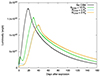 |
Fig. 8. Effect of different CSM radii on the bolometric light curves of single-star models. The black line represents the non-interacting reference models (Table 1, S1). In contrast, the green, light blue, and orange lines illustrate the effect of circumstellar matter with a radius of 10, 5, and 2 Rp, respectively. |
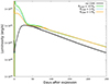 |
Fig. 9. Effect of different CSM radii on the bolometric light curves of binary models. The black line represents the non-interacting reference models (Table 2, B12). In contrast, the green, light blue, and orange lines illustrate the effect of circumstellar matter with a radius of 10, 5, and 2 Rp, respectively. |
To check the consistency of the interacting light curve models, we compared our results with the theoretical model published by Piro (2015). We calculated tp and Lp via Eqs. (6) and (7) applying the different CSM model parameters, and we then compared them with the simulation data. As a result, we obtained similar trends in both parameters, suggesting that our models are consistent. Although this qualitative check showed constancy, we were not able to determine exact values for these parameters as SNEC defines a nonconstant opacity profile. Thus, we were only able to determine tp and Lp to within a factor of the average opacity. Nevertheless, when we estimate κ for the different models as matching the theoretical calculations with model data, the average opacity varied between 0.03 − 0.2 cm2/g, which corresponds well with the integrated average opacity of stripped-envelope supernovae (Nagy 2018).
4. Comparison with observations
To test our hypotheses that a low-mass close CSM shell may cause strange light curve features (bumps, re-brightening, or steeper tail), we selected the reference explosion events. We chose three recent Type Ib/c supernovae (SN 2020oi, iPTF15dtg, and SN 2008D) classified as non-interacting SESNe and showed some irregularities in their LCs. Moreover, we also required these selected transients to have similar bolometric light curve features as constructed by our CSM-interacting models. To compare synthesized light curves with observational data, we needed to calculate the bolometric LCs of the selected supernovae. To do this, we used the same method as Nagy et al. (2014), which applies the trapezoidal rule for the integration over wavelength, assuming that the flux reaches zero at 2000 Å. However, as Nakar & Sari (2010) and Haynie & Piro (2021) pointed out, the LC could reach its first maximum at higher frequencies than optical by incomplete thermalization around the shock breakout. Thus, the luminosity of the first peak might be underestimated: This is the case for SN 2008D, but likely also for the other two SNe (see Gagliano et al. 2022, for SN 2020oi).
We mainly focused on the overall shape of the light curves because it may indicates whether the progenitor was a single star or was part of a binary system. It was therefore beyond the scope of this paper to determine the physical properties of these three supernovae. We just tried to recreate their generic LC features and shift the observed and model light curves together. Thus, we used the S1 (Table 1) single-star progenitor model for all three objects, and we adopted the B2 and B12 (Table 2) binary calculations for SN 2008D and SN 2020oi/iPTF15dtg, respectively. Nevertheless, we wished to ensure that our shifting method did not cause any systematic error that could alter our conclusions. To remove the limitations of our model grid, we therefore applied the Arnett model (Arnett 1982), where the relation between the ejecta mass and the explosion energy (M/Eexp2) approximately defines the width of the LC. When we scaled the previously published explosion energies (SN 2008D: Tanaka et al. 2009; iPTF15dtg: Taddia et al. 2016; SN 2020oi: Rho et al. 2021; Gagliano et al. 2022) according to this relation, we therefore only needed to shift our model light curves up or down for a comparison with the supernova data.
One of our chosen supernovae, SN 2020oi, was discovered on January 7, 2020, by the Zwicky Transient Facility (Forster et al. 2020) in M100, which is a nearby galaxy at a distance of 16.22 Mpc (Rho et al. 2021). Although this object was classified as a normal Type Ic, Horesh et al. (2020) and Maeda et al. (2021) suggested a possible interaction between the supernova ejecta and a supposed dense circumstellar material around the progenitor. Moreover, Gagliano et al. (2022) even showed that SN 2020oi exploded in a binary system. Thus, this recent transient seemed to be perfect for testing our interacting binary models.
In the top panel of Fig. 10 we compare our interacting binary model related to MCSM = 2 M⊙ and RCSM = 2 ⋅ Rp with the bolometric light curve of SN 2020oi generated from photometric data published by Rho et al. (2021). To show the resemblance between the two light curves better, we increased the initial nickel mass of the hydrodynamic model to 0.2 M⊙. Again, we note that we did not try to recreate the explosion parameters in detail. We only scaled the luminosities together to demonstrate what the shapes of the curves look like relative to each other. The synthesized light curves follow the same temporal evolution as the bolometric LC of SN 2020oi. To ensure that our interacting single-star scenario was not capable of recreating the light variation of SN 2020oi properly, we tried to find an acceptable model. We also show our most promising single-star model in the same panel of Fig. 10. Considering our results and the findings of Rho et al. (2021), Horesh et al. (2020), Gagliano et al. (2022), SN 2020oi might be an interacting SESN with a binary origin.
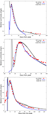 |
Fig. 10. Comparison of an interacting single-star (blue line) and an interacting binary (black line) model with the bolometric light curve (red circles) of SN 2020oi (top panel), iPTF15dtg (middle panel), and SN 200D (bottom panel), respectively. |
Our other chosen supernova was iPTF15dtg, discovered on November 7, 2015, by the Palomar Transient Factory with the 96 Mpixel mosaic camera CFH12K (Rahmer et al. 2008). It was located in an anonymous galaxy at a luminosity distance of about 232.0 Mpc (Taddia et al. 2016). Due to its high luminosity, iPTF15dtg was classified as a peculiar slow-rising Type Ic supernova. However, Jin et al. (2021) suggested that this transient was an interacting supernova with an assumed MCSM = 0.05 − 0.15 M⊙ circumstellar matter, which made it an ideal test object for our single-star models.
In the middle panel of Fig. 10 we compare our interacting single-star model related to MCSM = 0.05 M⊙ and RCSM = 5 ⋅ Rp with the bolometric light curve of the iPTF15dtg. We also scaled the luminosities together, and we obtained a reasonably good agreement with the bolometric LC of iPTF15dtg. To rule out a binary origin, we created interacting binary models to determine the most iPTF15dtg-like light curve shape, which is also plotted in the corresponding figure. Based on our results, it seems more feasible that this supernova originated from a single-star progenitor because our interacting binary models are unable to create the rising part of the LC peak.
Finally, we used the Type Ib supernova, SN 2008D discovered on January 9, 2008, in NGC 2770 (d = 27 Mpc) (Soderberg et al. 2008). It was originally detected with the Swift X-ray Telescope as an X-ray transient and appeared about 1.5 hours later in the optical images. Later, theoretical studies recommended extremely different scenarios to explain the observational features of SN 2008D. Some of them suggested a compact, energetic, and aspherical single-star explosion, where the ejecta collides with the circumstellar matter (e.g. Scully et al. 2023), while others preferred a binary origin (e.g. Brown & Lee 2008).
In the bottom panel of Fig. 10 we compare our scaled interacting single-star model related to MCSM = 0.1 M⊙ and RCSM = 10 ⋅ Rp with the bolometric light curve of the SN 2008D. Although the light curve does not follow the observed data, the shape of the modeled luminosities suggests that more detailed calculations may fit the light variation of SN 2008D properly. We also created interacting binary models to determine whether a progenitor that originated in a binary might produce a more closely SN 2008D-like LC (Fig. 10). The best-fitting model is related to a MIbc = 3.23 M⊙ progenitor with an MCSM = 2 M⊙ and RCSM = 2 ⋅ Rp circumstellar matter. The binary progenitor agrees with the light curve of SN 2008D after the maximum. However, since binary models cannot form the early slow-rising features of the LC peak, it seems unlikely that this explosion event originated from a binary progenitor. Single-star models also have a limitation in this case, however. Without more detailed calculations, we only assert that SN 2008D shows LC features that resemble those of a progenitor that originated in a single star, which suggests an interacting single-star precursor by chance. Thus, further modeling is necessary to evaluate this scenario and reveal the true nature of the progenitor and the circumstellar environment related to this supernova explosion.
5. Conclusions
We have investigated the effect of close low-mass CSM shells around stripped-envelope supernova progenitors interacting with the SN ejecta by analyzing their bolometric LCs. Based on this systematic examination of the synthesized light curves, we found substantial evidence favoring our hypotheses. Namely, the strange light curve features of Type Ib/c supernovae can be explained by circumstellar interaction. We are aware that without a detailed spectral analysis, we cannot be sure that our models generate typical Type Ib/c spectra. However, the low mass and low density of the CSM may suggest that the estimated configuration does not produce narrow He, C, and O lines in the spectra and might also explain SESNe that change their classification type in time.
We also found that the evolution of the bolometric light curves of our interacting single-star models is different than that of the binary progenitors, possibly due to their diverse initial 56Ni distribution. As presented above, the progenitor dependence can mainly be monitored at the early LCs: The main peak of the LC shifts and narrows for single stars, while the rise-time and width remain about the same for binary progenitors. On the other hand, this early behavior might also be a trace of an inflated progenitor, where the star has an extended low-density outer envelope in addition to a more compact and more massive inner region (e.g. Nagy & Vinkó 2016; Bersten et al. 2012). However, these inflated-progenitor models do not significantly affect the nickel-cobalt tail, unlike some of our CSM models, since the former ones cannot infer such high masses to modify the late-time LC features. Hence, a more massive circumstellar material is the key requirement to explain the observable luminosity excess (e.g., dumps or rebrightening) on the Ni-Co tail.
Nevertheless, our results suggest that the overall light curve features mainly depend on the compactness of the progenitor star, regardless of the mass of its remaining He layer, which agrees well with the finding of Woosley (2019). Moreover, this phenomenon results in major differences between the LCs of the distinct progenitor scenarios, regardless of their similar maximum luminosity (Fig. 5). Thus, this may indicate that the pre-supernova evolution of the exploding star can be estimated from the general physical properties of Type Ib/c light curves.
To test the main objectives of this study, we compared our models with observational data. From an empirical point of view, the bolometric LC of stripped-envelope supernovae with bumps or rebrightening are quite heterogeneous. Some of them (e.g. SN 2008D, SN 2014L, and iPTF15dtg) show a rapidly rising narrow peak that fades as fast as it increases, while others (e.g. SN 2003dh, SN 2019dge, and SN 2020oi) seem to miss the ascending part, but their LC peak is usually broader. The second group might be affected by an observational bias. However, as demonstrated earlier for SN 2020oi, it may suggest an interacting binary progenitor. On the other hand, the bolometric light curve features of the first group resemble our interacting single-star models despite the initial peak. However, this might also be an observational issue, as it seems to be a problem for some Type IIb supernovae, where we discover the supernova too late to catch the first peak, which is otherwise assumed to be a common feature for these objects. Moreover, according to our simulations, the first peak can only be detected a few days after the explosion, which leads to the nondetection of this feature in the case of certain Type Ib/c events. Thus, the absence of the first peak does not indicate a lack of CSM interaction.
Overall, our study indicates that a relatively thin, detached, dense circumstellar matter may explain the behavior of some Type Ib/c supernovae that show unusual light curve features. The models we obtained can recreate the basic LC characteristics of these events, but are unable to determine the exact physical properties of the CSM via fitting observational data. This is mainly due to the simplified structure of our CSM model and to the complex nature of the hydrodynamical calculations.
Data availability
MESA and SNEC, the software used to produce the simulations for this paper, are fully open-source codes available at https://github.com/MESAHub/ and https://stellarcollapse.org/index.php/SNEC.html, respectively. Most initial parameters to recreate our models are presented in tables or within the inlist published in https://zenodo.org/records/14760396. Data files, models, etc., will be shared with users upon reasonable request.
Acknowledgments
Special thanks to Takashi J. Moriya for the valuable suggestions and discussions that helped to improve this article. This project is supported by NKFIH/OTKA PD-134434 and FK-134432 grants of the National Research, Development and Innovation (NRDI) Office of Hungary. This project has received funding from the HUN-REN Hungarian Research Network.
References
- Andriesse, C. D., & Viotti, R. 1979, in Mass Loss and Evolution of O-Type Stars, eds. P. S. Conti, & C. W. H. De Loore, 83, 47 [NASA ADS] [CrossRef] [Google Scholar]
- Arnett, W. D. 1982, ApJ, 253, 785 [Google Scholar]
- Arnett, W. D., & Fu, A. 1989, ApJ, 340, 396 [NASA ADS] [CrossRef] [Google Scholar]
- Benetti, S., Zampieri, L., Pastorello, A., et al. 2018, MNRAS, 476, 261 [NASA ADS] [CrossRef] [Google Scholar]
- Bersten, M. C., Benvenuto, O., & Hamuy, M. 2011, ApJ, 729, 61 [NASA ADS] [CrossRef] [Google Scholar]
- Bersten, M. C., Benvenuto, O. G., Nomoto, K., et al. 2012, ApJ, 757, 31 [Google Scholar]
- Bersten, M. C., Tanaka, M., Tominaga, N., Benvenuto, O. G., & Nomoto, K. 2013, ApJ, 767, 143 [NASA ADS] [CrossRef] [Google Scholar]
- Brown, G. E., & Lee, C.-H. 2008, ArXiv e-prints [arXiv:0810.0912] [Google Scholar]
- Cao, Y., Kasliwal, M. M., Arcavi, I., et al. 2013, ApJ, 775, L7 [NASA ADS] [CrossRef] [Google Scholar]
- Chevalier, R. A., & Fransson, C. 2003, in Supernovae and Gamma-Ray Bursters, ed. K. Weiler, 598, 171 [NASA ADS] [CrossRef] [Google Scholar]
- Chevalier, R. A., & Fransson, C. 2006, ApJ, 651, 381 [NASA ADS] [CrossRef] [Google Scholar]
- Chugai, N. N., Chevalier, R. A., & Utrobin, V. P. 2007, ApJ, 662, 1136 [NASA ADS] [CrossRef] [Google Scholar]
- Clocchiatti, A., & Wheeler, J. C. 1997, ApJ, 491, 375 [Google Scholar]
- de Jager, C., Nieuwenhuijzen, H., & van der Hucht, K. A. 1988, A&AS, 72, 259 [NASA ADS] [Google Scholar]
- Dessart, L., Hillier, D. J., & Kuncarayakti, H. 2022, A&A, 658, A130 [NASA ADS] [CrossRef] [EDP Sciences] [Google Scholar]
- Forster, F., Pignata, G., Bauer, F. E., et al. 2020, TNSTR, 2020-67, 1 [Google Scholar]
- Fraser, M. 2020, R. Soc. Open Sci., 7, 200467 [NASA ADS] [CrossRef] [Google Scholar]
- Gagliano, A., Izzo, L., Kilpatrick, C. D., et al. 2022, ApJ, 924, 55 [Google Scholar]
- Georgy, C., Meynet, G., Walder, R., Folini, D., & Maeder, A. 2009, A&A, 502, 611 [NASA ADS] [CrossRef] [EDP Sciences] [Google Scholar]
- Glebbeek, E., Gaburov, E., de Mink, S. E., Pols, O. R., & Portegies Zwart, S. F. 2009, A&A, 497, 255 [NASA ADS] [CrossRef] [EDP Sciences] [Google Scholar]
- Hachinger, S., Mazzali, P. A., Taubenberger, S., et al. 2012, MNRAS, 422, 70 [NASA ADS] [CrossRef] [Google Scholar]
- Haynie, A., & Piro, A. L. 2021, ApJ, 910, 128 [NASA ADS] [CrossRef] [Google Scholar]
- Hiramatsu, D., Tsuna, D., Berger, E., et al. 2023, ApJ, 955, L8 [NASA ADS] [CrossRef] [Google Scholar]
- Ho, A. Y. Q., Goldstein, D. A., Schulze, S., et al. 2019, ApJ, 887, 169 [Google Scholar]
- Horesh, A., Sfaradi, I., Ergon, M., et al. 2020, ApJ, 903, 132 [NASA ADS] [CrossRef] [Google Scholar]
- Jermyn, A. S., Bauer, E. B., Schwab, J., et al. 2023, ApJS, 265, 15 [NASA ADS] [CrossRef] [Google Scholar]
- Jin, H., Yoon, S.-C., & Blinnikov, S. 2021, ApJ, 910, 68 [NASA ADS] [CrossRef] [Google Scholar]
- Jin, H., Yoon, S.-C., & Blinnikov, S. 2023, ApJ, 950, 44 [Google Scholar]
- Jung, M.-K., Yoon, S.-C., & Kim, H.-J. 2022, ApJ, 925, 216 [NASA ADS] [CrossRef] [Google Scholar]
- Kashi, A., & Michaelis, A. 2021, Galaxies, 10, 4 [NASA ADS] [CrossRef] [Google Scholar]
- Kochanek, C. S. 2019, MNRAS, 483, 3762 [Google Scholar]
- Kuncarayakti, H., Maeda, K., Dessart, L., et al. 2022, ApJ, 941, L32 [NASA ADS] [CrossRef] [Google Scholar]
- Kuncarayakti, H., Sollerman, J., Izzo, L., et al. 2023, A&A, 678, A209 [NASA ADS] [CrossRef] [EDP Sciences] [Google Scholar]
- Kuriyama, N., & Shigeyama, T. 2020, A&A, 635, A127 [NASA ADS] [CrossRef] [EDP Sciences] [Google Scholar]
- Limongi, M. 2017, in Handbook of Supernovae, eds. A. W. Alsabti, & P. Murdin, 513 [CrossRef] [Google Scholar]
- Lyman, J. D., Bersier, D., James, P. A., et al. 2016, MNRAS, 457, 328 [Google Scholar]
- Maeda, K., & Moriya, T. J. 2022, ApJ, 927, 25 [NASA ADS] [CrossRef] [Google Scholar]
- Maeda, K., Chandra, P., Matsuoka, T., et al. 2021, ApJ, 918, 34 [NASA ADS] [CrossRef] [Google Scholar]
- Mazzali, P. A., Sullivan, M., Pian, E., Greiner, J., & Kann, D. A. 2016, MNRAS, 458, 3455 [NASA ADS] [CrossRef] [Google Scholar]
- Mcley, L., & Soker, N. 2014, MNRAS, 445, 2492 [CrossRef] [Google Scholar]
- Moriya, T. J., & Maeda, K. 2012, ApJ, 756, L22 [NASA ADS] [CrossRef] [Google Scholar]
- Moriya, T., Tominaga, N., Blinnikov, S. I., Baklanov, P. V., & Sorokina, E. I. 2011, MNRAS, 415, 199 [NASA ADS] [CrossRef] [Google Scholar]
- Morozova, V., Piro, A. L., Renzo, M., et al. 2015, ApJ, 814, 63 [Google Scholar]
- Müller, T., Prieto, J. L., Pejcha, O., & Clocchiatti, A. 2017, ApJ, 841, 127 [Google Scholar]
- Nagy, A. P. 2018, ApJ, 862, 143 [Google Scholar]
- Nagy, A. P., & Vinkó, J. 2016, A&A, 589, A53 [NASA ADS] [CrossRef] [EDP Sciences] [Google Scholar]
- Nagy, A. P., Ordasi, A., Vinkó, J., & Wheeler, J. C. 2014, A&A, 571, A77 [NASA ADS] [CrossRef] [EDP Sciences] [Google Scholar]
- Nakar, E., & Sari, R. 2010, ApJ, 725, 904 [NASA ADS] [CrossRef] [Google Scholar]
- Nugis, T., & Lamers, H. J. G. L. M. 2000, A&A, 360, 227 [NASA ADS] [Google Scholar]
- Ouchi, R., Maeda, K., Anderson, J. P., & Sawada, R. 2021, ApJ, 922, 141 [CrossRef] [Google Scholar]
- Paczynski, B. 1983, ApJ, 267, 315 [CrossRef] [Google Scholar]
- Pastorello, A., Smartt, S. J., Mattila, S., et al. 2007, Nature, 447, 829 [NASA ADS] [CrossRef] [Google Scholar]
- Pauli, D., Oskinova, L. M., Hamann, W. R., et al. 2023, A&A, 673, A40 [NASA ADS] [CrossRef] [EDP Sciences] [Google Scholar]
- Paxton, B., Bildsten, L., Dotter, A., et al. 2011, ApJS, 192, 3 [Google Scholar]
- Paxton, B., Cantiello, M., Arras, P., et al. 2013, ApJS, 208, 4 [Google Scholar]
- Paxton, B., Marchant, P., Schwab, J., et al. 2015, ApJS, 220, 15 [Google Scholar]
- Paxton, B., Schwab, J., Bauer, E. B., et al. 2018, ApJS, 234, 34 [NASA ADS] [CrossRef] [Google Scholar]
- Paxton, B., Smolec, R., Schwab, J., et al. 2019, ApJS, 243, 10 [Google Scholar]
- Petrovic, J., Langer, N., & van der Hucht, K. A. 2005, A&A, 435, 1013 [NASA ADS] [CrossRef] [EDP Sciences] [Google Scholar]
- Piro, A. L. 2015, ApJ, 808, L51 [NASA ADS] [CrossRef] [Google Scholar]
- Quataert, E., Fernández, R., Kasen, D., Klion, H., & Paxton, B. 2016, MNRAS, 458, 1214 [NASA ADS] [CrossRef] [Google Scholar]
- Rahmer, G., Smith, R., Velur, V., et al. 2008, in Ground-based and Airborne Instrumentation for Astronomy II, eds. I. S. McLean, & M. M. Casali, SPIE Conf. Ser., 7014, 70144Y [NASA ADS] [Google Scholar]
- Reimers, D. 1975, Problems in Stellar Atmospheres and Envelopes, 229 [Google Scholar]
- Rho, J., Evans, A., Geballe, T. R., et al. 2021, ApJ, 908, 232 [NASA ADS] [CrossRef] [Google Scholar]
- Rodríguez, Ó., Maoz, D., & Nakar, E. 2023, ApJ, 955, 71 [CrossRef] [Google Scholar]
- Sana, H., de Mink, S. E., de Koter, A., et al. 2012, Science, 337, 444 [Google Scholar]
- Scully, B., Matzner, C. D., & Yalinewich, A. 2023, MNRAS, 525, 1562 [NASA ADS] [Google Scholar]
- Shao, Y., & Li, X.-D. 2016, ApJ, 833, 108 [NASA ADS] [CrossRef] [Google Scholar]
- Soderberg, A. M., Berger, E., Page, K. L., et al. 2008, Nature, 453, 469 [NASA ADS] [CrossRef] [Google Scholar]
- Sollerman, J., Fransson, C., Barbarino, C., et al. 2020, A&A, 643, A79 [NASA ADS] [CrossRef] [EDP Sciences] [Google Scholar]
- Soraisam, M., Matheson, T., Lee, C.-H., et al. 2022, ApJ, 926, L11 [NASA ADS] [CrossRef] [Google Scholar]
- Strotjohann, N. L., Ofek, E. O., Gal-Yam, A., et al. 2021, ApJ, 907, 99 [NASA ADS] [CrossRef] [Google Scholar]
- Taddia, F., Sollerman, J., Leloudas, G., et al. 2015, A&A, 547, A60 [Google Scholar]
- Taddia, F., Fremling, C., Sollerman, J., et al. 2016, A&A, 592, A89 [NASA ADS] [CrossRef] [EDP Sciences] [Google Scholar]
- Taddia, F., Stritzinger, M. D., Bersten, M., et al. 2018, A&A, 609, A136 [NASA ADS] [CrossRef] [EDP Sciences] [Google Scholar]
- Takei, Y., Tsuna, D., Ko, T., & Shigeyama, T. 2024, ApJ, 961, 67 [Google Scholar]
- Tanaka, M., Tominaga, N., Nomoto, K., et al. 2009, ApJ, 692, 1131 [NASA ADS] [CrossRef] [Google Scholar]
- Tsuna, D., & Takei, Y. 2023, PASJ, 75, L19 [NASA ADS] [CrossRef] [Google Scholar]
- Vamvatira-Nakou, C., Hutsemékers, D., Royer, P., et al. 2016, A&A, 588, A92 [NASA ADS] [CrossRef] [EDP Sciences] [Google Scholar]
- Vink, J. S. 2022, ARA&A, 60, 203 [NASA ADS] [CrossRef] [Google Scholar]
- Vink, J. S., de Koter, A., & Lamers, H. J. G. L. M. 2001, A&A, 369, 574 [NASA ADS] [CrossRef] [EDP Sciences] [Google Scholar]
- Wheeler, J. C., Chatzopoulos, E., Vinkó, J., & Tuminello, R. 2017, ApJ, 851, L14 [NASA ADS] [CrossRef] [Google Scholar]
- Woosley, S. E. 2019, ApJ, 878, 49 [Google Scholar]
- Woosley, S. E., Heger, A., Cumming, A., et al. 2004, ApJS, 151, 75 [NASA ADS] [CrossRef] [Google Scholar]
- Woosley, S. E., Sukhbold, T., & Kasen, D. N. 2021, ApJ, 913, 145 [NASA ADS] [CrossRef] [Google Scholar]
All Tables
All Figures
|
Fig. 1. Comparison of the initial density profile of a non-interacting and an interacting single-star model. The black line represents the non-interacting reference model, and the red line shows the total density profile of the same model with an added CSM profile. |
| In the text | |
|
Fig. 2. Comparison of the calculated bolometric light curves for interacting CSM models (MCSM = 2 M⊙, RCSM = 10 Rp ) with different abundances. The red curve represents the H-free CSM, and the black line shows a solar-like chemical composition. |
| In the text | |
|
Fig. 3. Comparison of calculated bolometric light curves with different ‘Bomb_mode’ options. The red curve represents ‘Bomb_mode =1’, where Eexp = ESN − Ebin, and the black lines show the fixed explosion energy option (‘Bomb_mode =2’). |
| In the text | |
|
Fig. 4. Comparison of single-star and binary models with a similar progenitor mass. The red and orange lines represent single-star models with 4.28 and 6.74 M⊙, and green and blue lines show binary calculations with 4.58 and 6.68 M⊙, respectively. |
| In the text | |
|
Fig. 5. Comparison of a single-star and a binary progenitor model calculated with MIbc and similar peak luminosities. |
| In the text | |
|
Fig. 6. Effect of a different CSM mass on the bolometric light curves of single-star models. The black line represents the non-interacting reference model (Table 1, S1). In contrast, the violet, dark blue, light blue, green, orange, and red lines illustrate the effect of circumstellar matter with a mass of 0.01, 0.05, 0.1, 0.5, 1, and 2 M⊙, respectively. |
| In the text | |
|
Fig. 7. Effect of a different CSM mass on the bolometric light curves of binary models. The black line represents the non-interacting reference model (Table 2, B12). In contrast, the violet, dark blue, light blue, green, orange, and red lines illustrate the effect of circumstellar matter with a mass of 0.01, 0.05, 0.1, 0.5, 1, and 2 M⊙, respectively. |
| In the text | |
|
Fig. 8. Effect of different CSM radii on the bolometric light curves of single-star models. The black line represents the non-interacting reference models (Table 1, S1). In contrast, the green, light blue, and orange lines illustrate the effect of circumstellar matter with a radius of 10, 5, and 2 Rp, respectively. |
| In the text | |
|
Fig. 9. Effect of different CSM radii on the bolometric light curves of binary models. The black line represents the non-interacting reference models (Table 2, B12). In contrast, the green, light blue, and orange lines illustrate the effect of circumstellar matter with a radius of 10, 5, and 2 Rp, respectively. |
| In the text | |
|
Fig. 10. Comparison of an interacting single-star (blue line) and an interacting binary (black line) model with the bolometric light curve (red circles) of SN 2020oi (top panel), iPTF15dtg (middle panel), and SN 200D (bottom panel), respectively. |
| In the text | |
Current usage metrics show cumulative count of Article Views (full-text article views including HTML views, PDF and ePub downloads, according to the available data) and Abstracts Views on Vision4Press platform.
Data correspond to usage on the plateform after 2015. The current usage metrics is available 48-96 hours after online publication and is updated daily on week days.
Initial download of the metrics may take a while.