| Issue |
A&A
Volume 687, July 2024
|
|
|---|---|---|
| Article Number | L20 | |
| Number of page(s) | 6 | |
| Section | Letters to the Editor | |
| DOI | https://doi.org/10.1051/0004-6361/202450440 | |
| Published online | 22 July 2024 | |
Letter to the Editor
Progenitor mass and ejecta asymmetry of supernova 2023ixf from nebular spectroscopy
1
Instituto de Astrofísica de La Plata, Paseo del Bosque s/n, 1900
Buenos Aires, Argentina
2
Facultad de Ciencias Astronómicas y Geofísicas Universidad Nacional de La Plata, Paseo del Bosque s/n B1900FWA, La Plata, Argentina
e-mail: This email address is being protected from spambots. You need JavaScript enabled to view it.
3
Kavli Institute for the Physics and Mathematics of the Universe (WPI), The University of Tokyo, Kashiwa, 277-8583
Chiba, Japan
4
Finnish Centre for Astronomy with ESO (FINCA), University of Turku, 20014
Turku, Finland
5
Tuorla Observatory, Department of Physics and Astronomy, University of Turku, 20014
Turku, Finland
6
Gemini Observatory/NSF’s NOIRLab, 670 N. A’ohoku Place, Hilo, HI, 96720
USA
Received:
18
April
2024
Accepted:
1
July
2024
Abstract
Context. Supernova (SN) 2023ixf was discovered in the galaxy M 101 in May 2023. Its proximity provided the scientific community an extremely valuable opportunity to study the characteristics of the SN and its progenitor. A point source detected on archival images and hydrodynamical modeling of the bolometric light curve have been used to constrain the former star’s properties. There is a significant variation in the published results regarding the initial mass of the progenitor. Nebular spectroscopy can be used to enhance our understanding of the SN and its progenitor.
Aims. We determined the SN progenitor mass by studying the first published nebular spectrum, taken 259 days after the explosion.
Methods. We analyzed the nebular spectrum taken with GMOS at the Gemini North Telescope. We identified typical emission lines, such as [O I], Hα, and [Ca II], among others. Some species’ line profiles show broad and narrow components, indicating two ejecta velocities and an asymmetric ejecta. We inferred the progenitor mass of SN 2023ixf by comparing its spectra with synthetic spectra and by measuring the forbidden oxygen doublet flux.
Results. Based on the flux ratio and the direct comparison with spectra models, the progenitor star of SN 2023ixf had a MZAMS between 12 and 15 M⊙. We find that using the [O I] doublet flux provides a less tight constraint on the progenitor mass. Our results agree with those from hydrodynamical modeling of the early light curve and pre-explosion image estimates that point to a relatively low-mass progenitor.
Key words: supernovae: general / supernovae: individual: SN 2023ixf
© The Authors 2024
 Open Access article, published by EDP Sciences, under the terms of the Creative Commons Attribution License (https://creativecommons.org/licenses/by/4.0), which permits unrestricted use, distribution, and reproduction in any medium, provided the original work is properly cited.
This article is published in open access under the Subscribe to Open model. This email address is being protected from spambots. You need JavaScript enabled to view it. to support open access publication.
1. Introduction
One key aspect of astrophysics is understanding the fate of massive stars and the origin of supernova (SN) explosions. Hydrogen-rich SNe, known as Type II SNe (SNe II), arise from the core collapse of stars more massive than about 8 M⊙ during the red supergiant phase, as confirmed through direct progenitor detections (Maund et al. 2005; Van Dyk et al. 2012; Smartt 2015). However, there is an apparent contradiction between theory and observations in the high-end range of SN-II progenitor masses. Direct detections appear to show a lack of progenitors more massive than 17 − 18 M⊙, while the theoretical limit should be around 25 − 30 M⊙ (Smartt 2015). Although several explanations have been proposed to explain this apparent discrepancy (Davies & Beasor 2018), it remains of the utmost importance to determine the masses of more SN-II progenitors.
Apart from direct detections on pre-explosions images, which is a powerful method albeit one limited to the nearby Universe, there are other more indirect ways to derive progenitor properties. One such method is through modeling of the nebular-phase spectra. Once the plateau phase ends, most of the SN ejecta become transparent and the spectral emission originates from regions near the former stellar core. Analysis of the nebular spectrum reveals properties of the core, such as its mass (Jerkstrand et al. 2012; Kuncarayakti et al. 2015; Dessart et al. 2021). The stellar-core mass is in turn indicative of the initial mass with which the star was formed. Furthermore, the shape of the emission lines provides information about the distribution of the innermost ejecta and thus can give hints as to the possible asymmetries that may occur during the explosion (Taubenberger et al. 2009; Fang et al. 2022).
The Type II SN 2023ixf, discovered in the galaxy M 101, is one of the most nearby SNe discovered in the last few decades. Due to its proximity, it piqued the interest of professional and amateur astronomers alike. A veritable wealth of articles and communications have been published since its discovery in May 2023. Part of these analyses focused on early-time time observations across the electromagnetic spectrum. The presence of a dense circumstellar material (CSM) surrounding the SN was revealed by early-on high ionization “flash” spectral lines (Perley et al. 2023; Jacobson-Galán et al. 2023; Smith et al. 2023; Bostroem et al. 2023; Hiramatsu et al. 2023; Teja et al. 2023), along with an early excess in the light curve, especially in the ultraviolet range (Jacobson-Galán et al. 2023; Hosseinzadeh et al. 2023; Teja et al. 2023; Martinez et al. 2024), as well as in X-ray, radio, and polarimetry observations (Grefenstette et al. 2023; Berger et al. 2023; Vasylyev et al. 2023). Several groups analyzed pre-explosion observations of the SN site from the Hubble Space Telescope and the Large Binocular Telescope in the optical, and the Spitzer Space Telescope in the infrared. These works find a putative progenitor object at the SN location whose spectral energy distribution (SED) is compatible with it being a dust-enshrouded red supergiant star. However, estimates of the zero-age main sequence (ZAMS) progenitor mass differ widely, from MZAMS ≈ 8 M⊙ to MZAMS ≈ 18 M⊙ (Qin et al. 2023,  ; Van Dyk et al. 2024, 12 − 15 M⊙; Kilpatrick et al. 2023, 11 ± 2 M⊙; Jencson et al. 2023, 17 ± 4 M⊙; Xiang et al. 2024,
  ; Neustadt et al. 2024, 9 − 14 M⊙). This discrepancy can be attributed to the different SEDs inferred by the authors and the variety of models employed to reproduce the progenitor star emission. Moreover, high near-infrared emission indicates the presence of substantial amounts of dust. Its modeling and inferred parameters vary, leading to a discrepancy in the derived extinction suffered by the progenitor. Additional analyses of the stellar populations in the vicinity of the SN provided estimates of MZAMS = 17 − 19 M⊙ (Niu et al. 2023) and MZAMS ≈ 22 M⊙ (Liu et al. 2023). Soraisam et al. (2023) found a progenitor mass of MZAMS = 20 ± 4 M⊙ by interpreting the observed variability of the pre-SN source in the infrared observations as being due to the pulsational instability of an M-type star. Independently of the pre-explosion observations, Bersten et al. (2024) performed hydrodynamical modeling of the bolometric light curve and photospheric velocity evolution and were able to constrain the progenitor mass to MZAMS < 15 M⊙.
In this work we present the first nebular spectrum of SN 2023ixf in an attempt to constrain the progenitor mass using independent information. The spectrum also serves to provide some insights into the internal structure of the SN ejecta through line profile analysis. Section 2 provides a description of the observational data. In Sect. 3 we analyze the nebular spectrum properties, and we estimate a progenitor mass in Sect. 4. Our conclusions are summarized in Sect. 5.
2. Observations, reddening, and distance
The spectrum presented in this work was obtained with the Gemini Multi-Object Spectrograph (GMOS; Hook et al. 2004) mounted on the Gemini North Telescope (Program GN-2024A-Q-139, PI Andrews). The observations were divided into four 900 s exposures in long-slit mode with R400 grating. The data were processed with standard procedures using the Image Reduction and Analysis Facility (IRAF) Gemini package. Flux calibration was performed with a baseline standard observation. The spectrum resolution is ≈ 10 Å (≈500 km s−1 at 6000 Å). Adopting the explosion time at JD = 2460083.25 (Hosseinzadeh et al. 2023), the spectrum phase is 259 days after the explosion.
The redshift published in the NASA/IPAC Extragalactic Database1 (NED) for the host galaxy and used in this work is 0.0008. We additionally adopted a distance to M 101 of 6.85 ± 0.15 Mpc (Riess et al. 2022) and a Milky Way reddening of E(B − V)MW = 0.008 mag (Schlafly & Finkbeiner 2011). Reddening in the host galaxy was estimated by Lundquist et al. (2023) to be E(B − V)Host = 0.031 mag. We applied the extinction correction by using a standard extinction law (Cardelli et al. 1989) with RV = 3.1, and thus the total E(B − V)Total = 0.039 mag.
3. Spectral properties
The nebular spectrum of SN 2023ixf is presented in Fig. 1, in comparison with two prototypical Type IIP SNe, SN 1999em at 230 d (Leonard et al. 2002) and SN 2004et at 253 d (Sahu et al. 2006). Typical spectral features of SNe II at this phase are seen in the spectrum, most prominently the emissions from Hα, [O I]λλ6300, 6364, and [Ca II]λλ7291, 7324. Also identifiable are emission lines due to Mg I]λ4571 and the Ca infrared triplet (Ca IIλλ8498,8542,8662), and the P-Cygni profile due to the Na I D doublet (Na Iλλ5890,5895). No emission line is identifiable as Hβ. The [O I] feature appears stronger relative to Hα and the [Ca II] doublet as compared with SN 1999em and SN 2004et (see more on this in Sect. 4). Except for the [Ca II] doublet, the most prominent lines appear more blueshifted in SN 2023ixf than in its counterparts.
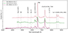 |
Fig. 1. Nebular spectra of SN 2023ixf compared with those of SN 1999em (Leonard et al. 2002) and SN 2004et (Sahu et al. 2006) at similar phases. The spectra are corrected for redshift and not extinction. Prominent emission features are indicated with gray vertical lines. |
Compared with the sample of Type II-P SNe from Silverman et al. (2017), we find that the emission lines appear in general broader in SN 2023ixf than in the other objects, except for SN 1992ad and SN 1993K. This is especially true in the case of Hα, which in SN 2023ixf shows a complex profile. This is discussed further in Sects. 3.1 and 3.2.
3.1. Line profiles
As shown in Fig. 1, most emission lines appear blueshifted in SN 2023ixf except for [Ca II] λλ7291, 7324, which is centered nearly at rest. The line profiles of the main spectral features are shown in detail in Fig. 2, and the following line velocities and full widths at half maximum (FWHMs) are summarized in Table 1. In the case of Hα, the profile can be decomposed into two components, a wide one (with FWHM = 5300 km s−1) centered at rest and an intermediate-width one (FWHM = 1600 km s−1) shifted by −1800 km s−1.
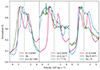 |
Fig. 2. Line profiles of several emission lines in 2023ixf. |
Details of the line shifts and FWHMs measured for the main emission lines.
The [O I] λλ6300, 6364 feature exhibits the double-peak profile that is typically seen in nebular spectra of core-collapse SNe (Maeda et al. 2008; Modjaz et al. 2008; Taubenberger et al. 2009). Recent three-dimensional modeling performed by Van Baal et al. (2023) was able to reproduce these asymmetric line profiles based on the viewing angle. The peaks are displaced roughly symmetrically relative to 6300 Å. Both emission peaks appear to have complex profiles that can be decomposed into a wider (FWHM ≈ 2000 km s−1) and a narrower (FWHM ≈ 500 km s−1)2 component, as shown in Fig. 3. The centers of the wider components are separated by ≈2500 km s−1 and are at −1100 km s−1 and 1400 km s−1, respectively. The narrower peaks are slightly farther apart, with a separation of ≈3000 km s−1, and both peaks are shifted by −1700 km s−1 and 1300 km s−1, respectively. We note that a separation of ≈3000 km s−1 is roughly equal to that between the [O I] λ6300 and [O I] λ6364 lines that produce this feature. Similar blueshifts in [O I] and Hα were observed in SN 2007it (Andrews et al. 2011). Furthermore, a multiple-component feature in [O I] has been seen before in SN 2016gkg, where it was attributed to multiple distinct kinematic components of material at low and high velocities (Kuncarayakti et al. 2020). Hypotheses for the material distribution in SN 2023ixf are discussed in Sect. 3.2.
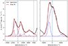 |
Fig. 3. Fitting of the [O I] doublet and Hα profiles. Dashed blue lines indicate the rest wavelength for 6300 Å and 6564 Å in the left and right panels, respectively, and the dashed gray line indicates the rest wavelength for 6456 Å, which could be associated with O I or Fe II. The thin lines show the individual Gaussian components. See Sect. 3.2 for the interpretation of the line components. |
To fit the four components that we attribute to [O I] λλ6300, 6364, we subtracted an additional set of wide and narrow Gaussian profiles centered at 6413 Å (see Fig. 3, left panel). This feature may also be present in the spectrum of SN 1999em (see Fig. 1). According to the National Institute of Standards and Technology3 (NIST) spectroscopic line atlas, it may be attributed to Fe IIλ6456 or to O Iλ6456 blueshifted by ≈2000 km s−1. However, this identification is not clear as the profile may be affected by a redshifted remainder absorption component of the Hα line. There is no clear explanation for this permitted line. Furthermore, we do not recognize this feature in the sample of nebular spectra from Silverman et al. (2017).
Two emission features appear that may be [O I]λ5577 and O Iλ7774, although with a blueshift of 1500 km s−1. This is shown in Fig. 2 (central panel). If the identifications are correct, the blueshifts are similar to those of the [O I]λλ63006364 lines. Mg I]λ4571 and Na I D are clearly identifiable in the spectrum and are both blueshifted by ≈1000 km s−1, roughly similar to the other lines. Na I D shows a broad profile and an absorption produced by the interstellar medium on top.
3.2. Ejecta geometry
Line shifts and widths provide information on the distribution of elements within the ejecta. For this purpose, we fit the [O I] doublet and the Hα emissions using multiple Gaussian profiles, as shown in Fig. 3. The [O I] double-peaked profile is an indicator of an asymmetry in the ejecta (Kuncarayakti et al. 2020; Fang et al. 2022). It is also noticeable that the [Ca II] doublet is centered at the rest wavelength. Thus, the disposition of the inner material could be an axisymmetric oxygen-rich torus surrounding a bipolar calcium region, similar to the scenario proposed by Fang et al. (2024, see their Fig. 3). The general blueshift common to all species supports this hypothesis, meaning that we may be mostly seeing the torus’s near side, with the far side being mostly obscured. From this line of sight, the calcium presents a symmetric distribution at a nearly perpendicular plane, producing a rest-centered feature in the spectrum. In addition to this, an outer, roughly spherical, high-velocity H-rich material must be responsible for the wide, rest-centered Hα component. Nevertheless, the two global, intrinsically different emitting regions of the ejecta, associated with the low and high velocities, may be challenging to explain in the context of the mechanism of the explosion, which takes place deep in the core. Here we highlight that the double-component (broad + narrow) line profile possibly occurs in all ejecta layers, from the outermost parts (H) down to the inner layers (O, Na, and Mg) and the core (Ca).
Another hypothesis that may explain these peculiar line profiles is the presence of an asymmetric or clumpy CSM that slows parts of the ejecta and thus produces narrow, blueshifted line components. Moreover, the presence of CSM surrounding the SN has already been proposed for SN 2023ixf (e.g., Bostroem et al. 2023; Jacobson-Galán et al. 2023; Martinez et al. 2024). The extended, H-rich envelope is mainly unaffected and is seen as a rest-centered profile, while a small part of the hydrogen and the regions rich in other elements are mostly affected by the CSM slowdown.
4. Progenitor mass
Nebular SN spectra are useful indicators of the progenitor mass. The flux of the [O I]λλ6300, 6364 feature has been proposed as an indicator of CO core mass by proxy of the O mass in the core (Uomoto 1986; Jerkstrand et al. 2014). Given that absolute fluxes can be affected by errors in the spectral calibration or in the distance and extinction estimations, the flux ratios of [O I] λλ6300, 6364 over [Ca II] λλ7291, 7324 have been proposed as more robust indicators of the progenitor mass (Fransson & Chevalier 1989; Fang et al. 2022). The relation between the [O I]/[Ca II] flux ratio and the progenitor ZAMS mass is seen in the model nebular spectra from Jerkstrand et al. (2014). We derived a progenitor mass estimate by means of line fluxes and flux ratios, and by direct comparison with available model spectra.
In Fig. 4 we show the 259 d spectrum of SN 2023ixf and the modeled spectra computed by Jerkstrand et al. (2014) for SNe II at a similar age and for varying progenitor masses. The model spectra were scaled to match the distance to SN 2023ixf. A scaling factor of 1.15 was applied to the observed spectrum in order to match the synthetic VRI magnitudes with the observed ones available from the American Association of Variable Star Observers (AAVSO4) International Database. The value was calculated by taking an average of the scaling factor for each filter. The figure shows that the observed spectrum has suppressed emission of permitted lines from Hα and the Ca II infrared triplet as compared with all of the modeled spectra. Nevertheless, if one compares the emissions due to [O I] and [Ca II], the modeled spectra from 12 to 15 M⊙ progenitors provide the closest matches to the observations.
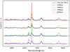 |
Fig. 4. SN 2023ixf at 259 d compared to nebular spectra models from Jerkstrand et al. (2014) at 250 d. |
In terms of the [O I]/[Ca II] flux ratio, the value obtained from the observed spectrum is 0.51. Compared with the ratios of 0.35, 0.60, 1.18, and 1.74 obtained from the modeled spectra with 12, 15, 19, and 25 M⊙, respectively, the result is indicative of a ZAMS progenitor mass between 12 and 15 M⊙. Furthermore, high-mass progenitors with MZAMS ≳ 19 M⊙ are disfavored based on this comparison.
We also considered the nebular spectra models from Dessart et al. (2021) to double-check this result. Although the epochs differ by about 100 days, as the available models are calculated for 360 days post-explosion, the oxygen-to-calcium ratio in the spectra models from Jerkstrand et al. (2014) does not show a significant time variation. The measured ratio value for SN 2023ixf is also consistent with progenitors with a ZAMS mass below 15 M⊙ based on measurements performed on the models from Dessart et al. (2021). The direct comparison also suggests a relatively low-mass progenitor, but we do not show it here as the nebular spectrum evolves significantly within 100 days. Further observations will enable us to use these models with more accuracy.
Another way of estimating the progenitor mass comes from the direct measurement of the [O I] doublet flux, which constrains the minimum oxygen mass responsible for such emission. This mass is linked to the progenitor mass by theoretical oxygen production yields. This procedure is detailed in Jerkstrand et al. (2014) and has been used as an independent way of estimating the progenitor mass (e.g., Sahu et al. 2011; Kuncarayakti et al. 2015). As mentioned before, the main uncertainties of this method lie in the absolute flux calibration (affected by the reddening correction and photometry scaling).
Assuming the emission with a peak at 5550 Å is [O I]λ5577 blueshifted by ≈1500 km s−1, we can establish only a lower limit for the flux, as the continuum is not clear and the line might be blended with the [Fe I]λ5501 line. The lower limit for the material temperature in this case would be 3700 K (Jerkstrand et al. 2014). The oxygen doublet flux is 2.38 × 10⁻¹³ erg s−1 cm−2, giving an oxygen mass of 0.5 M⊙. We assume this is the total mass that produces the measured flux. According to the oxygen production yields published by Nomoto et al. (1997) and Limongi & Chieffi (2003), the progenitor must have been a star with a mass of less than 17 M⊙. If we consider the production yields provided by Rauscher et al. (2002) and Sukhbold et al. (2016), the progenitor mass is well below 15 M⊙. Because of the uncertainties involved in this last method (in the absolute flux calibration and the temperature determination; see Jerkstrand 2017), we prefer the former approach (i.e., the one based on direct model comparison and flux ratios) to constrain the progenitor mass. We thus conclude that the progenitor must have been a star with a ZAMS mass between 12 and 15 M⊙.
5. Conclusions
We present the first nebular spectrum of SN 2023ixf published in the literature, taken 259 days after the explosion. The observations were obtained with the Gemini North Telescope using GMOS. The spectrum was used to examine the inner regions of the ejecta through line profiles and to determine the progenitor mass following a procedure independent of those previously published for this SN.
The spectrum shows the typical emission lines seen in a Type II SN resulting from the elements hydrogen, oxygen, calcium, sodium, and magnesium. In comparison with other Type II SNe, SN 2023ixf presents a weaker Hα emission, and no Hβ is recognizable. The [O I] doublet is blueshifted and shows a double-peaked profile. This is a sign of a nonspherical ejecta and may be interpreted as a torus-shaped emitting region. By fitting the line, we distinguished two wide components and two narrow components, also distinguishable as intermediate line peaks in the Hα profile and other lines as well. This feature, also detected in Mg I]λ4571 and Na I D, is attributed to a low-velocity ejecta component, caused either by two distinct ejecta regions or by parts of the material being partly slowed by an asymmetric or clumpy CSM. A wide Hα component is rest-centered and must be produced by an outer, roughly spherical, H-rich material.
The main result of our work is the estimation of the progenitor mass from the nebular spectrum. Via spectral comparison with models by Jerkstrand et al. (2014), we find that the progenitor mass was between 12 and 15 M⊙. We confirmed this by comparing the [O I]/[Ca II] flux ratio of the SN 2023ixf spectrum and those of the models. We also derived an upper limit of 15 − 17 M⊙ for the progenitor mass based on the [O I] flux. However, this result is less constraining and less reliable than the comparison with model spectra. Our derived mass is in agreement with the estimates of Bersten et al. (2024) based on hydrodynamical modeling and those of Kilpatrick et al. (2023), Xiang et al. (2024), Van Dyk et al. (2024), and Neustadt et al. (2024) based on pre-explosion images.
The width of these narrower lines is near the spectral resolution achieved by the data, so it may be considered an upper limit to the actual width.
Acknowledgments
We thank Dave Sand and Jeniveve Pearson, CoI’s for the Gemini Program GN-2024A-Q-139, for sharing the observational data. We thank the Gemini Observatory for encouraging fluid group interaction between Programs GN-2024A-Q-139 and GN-2024A-Q-309 teams. H.K. was funded by the Research Council of Finland projects 324504, 328898, and 353019. We acknowledge with thanks the variable star observations from the AAVSO International Database contributed by observers worldwide and used in this research. Based on observations obtained at the international Gemini Observatory (GN-2024A-Q-139, PI: Andrews), a program of NSF’s NOIRLab, which is managed by the Association of Universities for Research in Astronomy (AURA) under a cooperative agreement with the National Science Foundation. On behalf of the Gemini Observatory partnership: the National Science Foundation (United States), National Research Council (Canada), Agencia Nacional de Investigación y Desarrollo (Chile), Ministerio de Ciencia, Tecnología e Innovación (Argentina), Ministério da Ciência, Tecnologia, Inovações e Comunicações (Brazil), and Korea Astronomy and Space Science Institute (Republic of Korea). This work was enabled by observations made from the Gemini North telescope, located within the Maunakea Science Reserve and adjacent to the summit of Maunakea. We are grateful for the privilege of observing the Universe from a place that is unique in both its astronomical quality and its cultural significance.
References
- Andrews, J. E., Sugerman, B. E. K., Clayton, G. C., et al. 2011, ApJ, 731, 47 [NASA ADS] [CrossRef] [Google Scholar]
- Berger, E., Keating, G. K., Margutti, R., et al. 2023, ApJ, 951, L31 [NASA ADS] [CrossRef] [Google Scholar]
- Bersten, M. C., Orellana, M., Folatelli, G., et al. 2024, A&A, 681, L18 [NASA ADS] [CrossRef] [EDP Sciences] [Google Scholar]
- Bostroem, K. A., Pearson, J., Shrestha, M., et al. 2023, ApJ, 956, L5 [NASA ADS] [CrossRef] [Google Scholar]
- Cardelli, J. A., Clayton, G. C., & Mathis, J. S. 1989, ApJ, 345, 245 [Google Scholar]
- Davies, B., & Beasor, E. R. 2018, MNRAS, 474, 2116 [NASA ADS] [CrossRef] [Google Scholar]
- Dessart, L., Hillier, D. J., Sukhbold, T., Woosley, S. E., & Janka, H. T. 2021, A&A, 652, A64 [NASA ADS] [CrossRef] [EDP Sciences] [Google Scholar]
- Fang, Q., Maeda, K., Kuncarayakti, H., et al. 2022, ApJ, 928, 151 [NASA ADS] [CrossRef] [Google Scholar]
- Fang, Q., Maeda, K., Kuncarayakti, H., & Nagao, T. 2024, Nat. Astron., 8, 111 [Google Scholar]
- Fransson, C., & Chevalier, R. A. 1989, ApJ, 343, 323 [NASA ADS] [CrossRef] [Google Scholar]
- Grefenstette, B. W., Brightman, M., Earnshaw, H. P., Harrison, F. A., & Margutti, R. 2023, ApJ, 952, L3 [NASA ADS] [CrossRef] [Google Scholar]
- Hiramatsu, D., Tsuna, D., Berger, E., et al. 2023, ApJ, 955, L8 [NASA ADS] [CrossRef] [Google Scholar]
- Hook, I. M., Jørgensen, I., Allington-Smith, J. R., et al. 2004, PASP, 116, 425 [NASA ADS] [CrossRef] [Google Scholar]
- Hosseinzadeh, G., Farah, J., Shrestha, M., et al. 2023, ApJ, 953, L16 [NASA ADS] [CrossRef] [Google Scholar]
- Jacobson-Galán, W. V., Dessart, L., Margutti, R., et al. 2023, ApJ, 954, L42 [CrossRef] [Google Scholar]
- Jencson, J. E., Pearson, J., Beasor, E. R., et al. 2023, ApJ, 952, L30 [NASA ADS] [CrossRef] [Google Scholar]
- Jerkstrand, A. 2017, in Handbook of Supernovae, eds. A. W. Alsabti, & P. Murdin, 795 [CrossRef] [Google Scholar]
- Jerkstrand, A., Fransson, C., Maguire, K., et al. 2012, A&A, 546, A28 [NASA ADS] [CrossRef] [EDP Sciences] [Google Scholar]
- Jerkstrand, A., Smartt, S. J., Fraser, M., et al. 2014, MNRAS, 439, 3694 [Google Scholar]
- Kilpatrick, C. D., Foley, R. J., Jacobson-Galán, W. V., et al. 2023, ApJ, 952, L23 [NASA ADS] [CrossRef] [Google Scholar]
- Kuncarayakti, H., Maeda, K., Bersten, M. C., et al. 2015, A&A, 579, A95 [CrossRef] [EDP Sciences] [Google Scholar]
- Kuncarayakti, H., Folatelli, G., Maeda, K., et al. 2020, ApJ, 902, 139 [CrossRef] [Google Scholar]
- Leonard, D. C., Filippenko, A. V., Gates, E. L., et al. 2002, PASP, 114, 35 [Google Scholar]
- Limongi, M., & Chieffi, A. 2003, ApJ, 592, 404 [CrossRef] [Google Scholar]
- Liu, C., Chen, X., Er, X., et al. 2023, ApJ, 958, L37 [NASA ADS] [CrossRef] [Google Scholar]
- Lundquist, M., O’Meara, J., & Walawender, J. 2023, Trans. Name Server AstroNote, 160, 1 [NASA ADS] [Google Scholar]
- Maeda, K., Kawabata, K., Mazzali, P. A., et al. 2008, Science, 319, 1220 [NASA ADS] [CrossRef] [Google Scholar]
- Martinez, L., Bersten, M. C., Folatelli, G., Orellana, M., & Ertini, K. 2024, A&A, 683, A154 [NASA ADS] [CrossRef] [EDP Sciences] [Google Scholar]
- Maund, J. R., Smartt, S. J., & Danziger, I. J. 2005, MNRAS, 364, L33 [NASA ADS] [CrossRef] [Google Scholar]
- Modjaz, M., Kirshner, R. P., Blondin, S., Challis, P., & Matheson, T. 2008, ApJ, 687, L9 [NASA ADS] [CrossRef] [Google Scholar]
- Neustadt, J. M. M., Kochanek, C. S., & Smith, M. R. 2024, MNRAS, 527, 5366 [Google Scholar]
- Niu, Z., Sun, N.-C., Maund, J. R., et al. 2023, ApJ, 955, L15 [NASA ADS] [CrossRef] [Google Scholar]
- Nomoto, K., Hashimoto, M., Tsujimoto, T., et al. 1997, Nucl. Phys. A, 616, 79 [NASA ADS] [CrossRef] [Google Scholar]
- Perley, D. A., Gal-Yam, A., Irani, I., & Zimmerman, E. 2023, Trans. Name Server AstroNote, 119, 1 [NASA ADS] [Google Scholar]
- Qin, Y. J., Zhang, K., Bloom, J., et al. 2023, ArXiv e-prints [arXiv:2309.10022] [Google Scholar]
- Rauscher, T., Heger, A., Hoffman, R. D., & Woosley, S. E. 2002, ApJ, 576, 323 [Google Scholar]
- Riess, A. G., Yuan, W., Macri, L. M., et al. 2022, ApJ, 934, L7 [NASA ADS] [CrossRef] [Google Scholar]
- Sahu, D. K., Anupama, G. C., Srividya, S., & Muneer, S. 2006, MNRAS, 372, 1315 [Google Scholar]
- Sahu, D. K., Gurugubelli, U. K., Anupama, G. C., & Nomoto, K. 2011, MNRAS, 413, 2583 [NASA ADS] [CrossRef] [Google Scholar]
- Schlafly, E. F., & Finkbeiner, D. P. 2011, ApJ, 737, 103 [Google Scholar]
- Silverman, J. M., Pickett, S., Wheeler, J. C., et al. 2017, MNRAS, 467, 369 [NASA ADS] [Google Scholar]
- Smartt, S. J. 2015, PASA, 32, e016 [NASA ADS] [CrossRef] [Google Scholar]
- Smith, N., Pearson, J., Sand, D. J., et al. 2023, ApJ, 956, 46 [NASA ADS] [CrossRef] [Google Scholar]
- Soraisam, M. D., Szalai, T., Van Dyk, S. D., et al. 2023, ApJ, 957, 64 [NASA ADS] [CrossRef] [Google Scholar]
- Sukhbold, T., Ertl, T., Woosley, S. E., Brown, J. M., & Janka, H. T. 2016, ApJ, 821, 38 [NASA ADS] [CrossRef] [Google Scholar]
- Taubenberger, S., Valenti, S., Benetti, S., et al. 2009, MNRAS, 397, 677 [NASA ADS] [CrossRef] [Google Scholar]
- Teja, R. S., Singh, A., Basu, J., et al. 2023, ApJ, 954, L12 [NASA ADS] [CrossRef] [Google Scholar]
- Uomoto, A. 1986, ApJ, 310, L35 [NASA ADS] [CrossRef] [Google Scholar]
- Van Baal, B. F. A., Jerkstrand, A., Wongwathanarat, A., & Janka, H.-T. 2023, MNRAS, 523, 954 [NASA ADS] [CrossRef] [Google Scholar]
- Van Dyk, S. D., Cenko, S. B., Poznanski, D., et al. 2012, ApJ, 756, 131 [NASA ADS] [CrossRef] [Google Scholar]
- Van Dyk, S. D., Srinivasan, S., Andrews, J. E., et al. 2024, ApJ, 968, 27 [NASA ADS] [CrossRef] [Google Scholar]
- Vasylyev, S. S., Yang, Y., Filippenko, A. V., et al. 2023, ApJ, 955, L37 [NASA ADS] [CrossRef] [Google Scholar]
- Xiang, D., Mo, J., Wang, L., et al. 2024, Sci. China Phys. Mech. Astron., 67, 219514 [NASA ADS] [CrossRef] [Google Scholar]
All Tables
All Figures
|
Fig. 1. Nebular spectra of SN 2023ixf compared with those of SN 1999em (Leonard et al. 2002) and SN 2004et (Sahu et al. 2006) at similar phases. The spectra are corrected for redshift and not extinction. Prominent emission features are indicated with gray vertical lines. |
| In the text | |
|
Fig. 2. Line profiles of several emission lines in 2023ixf. |
| In the text | |
|
Fig. 3. Fitting of the [O I] doublet and Hα profiles. Dashed blue lines indicate the rest wavelength for 6300 Å and 6564 Å in the left and right panels, respectively, and the dashed gray line indicates the rest wavelength for 6456 Å, which could be associated with O I or Fe II. The thin lines show the individual Gaussian components. See Sect. 3.2 for the interpretation of the line components. |
| In the text | |
|
Fig. 4. SN 2023ixf at 259 d compared to nebular spectra models from Jerkstrand et al. (2014) at 250 d. |
| In the text | |
Current usage metrics show cumulative count of Article Views (full-text article views including HTML views, PDF and ePub downloads, according to the available data) and Abstracts Views on Vision4Press platform.
Data correspond to usage on the plateform after 2015. The current usage metrics is available 48-96 hours after online publication and is updated daily on week days.
Initial download of the metrics may take a while.