| Issue |
A&A
Volume 696, April 2025
|
|
|---|---|---|
| Article Number | L12 | |
| Number of page(s) | 7 | |
| Section | Letters to the Editor | |
| DOI | https://doi.org/10.1051/0004-6361/202452327 | |
| Published online | 11 April 2025 | |
Letter to the Editor
Spectropolarimetric modeling of interacting Type II supernovae. Application to early-time observations of SN 1998S
1
Institut d’Astrophysique de Paris, CNRS-Sorbonne Université, 98 bis boulevard Arago, F-75014 Paris, France
2
Department of Astronomy, San Diego State University, San Diego, CA 92182-1221, USA
3
Department of Astronomy, University of California, Berkeley, CA 94720-3411, USA
4
Department of Physics and Astronomy & Pittsburgh Particle Physics, Astrophysics, and Cosmology Center (PITT PACC), University of Pittsburgh, 3941 O’Hara Street, Pittsburgh, PA 15260, USA
⋆ Corresponding author; This email address is being protected from spambots. You need JavaScript enabled to view it.
Received:
20
September
2024
Accepted:
19
March
2025
Abstract
High-cadence surveys of the sky are revealing that a large fraction of red-supergiant (RSG) stars, which are the progenitors of Type II-Plateau (II-P) supernovae (SNe), explode within circumstellar material (CSM). Such Type II SNe exhibit a considerable diversity, with interaction signatures lasting from hours to days. As a result, they might merge with the Type IIn subclass, for which longer duration interaction typically occurs. To tackle this growing sample of transients and to understand the pre-SN mass loss histories of RSGs, we used the highest quality, spectropolarimetric observations of a young Type IIn SN taken to date. Specifically, we used those of SN 1998S at ∼5 days (d) after explosion. We designed an approach based on a combination of radiation hydrodynamics with HERACLES and polarized radiative transfer with CMFGEN and LONG_POL. The adopted asymmetries are based on a latitudinal, depth- and time-independent scaling of the density of 1D models of Type II SNe interacting with CSM (e.g., model r1w6b with a “wind” mass-loss rate of 0.01 M⊙ yr−1 used for SN 2023ixf). For a pole-to-equator density ratio of 5, we find that the polarization reaches (and then remains at each specific level for several days) a maximum value of 1.0, 1.4, and 1.8% as the CSM extent is changed from 6, to 8, and 10 × 1014 cm. The polarization is independent of wavelength, apart from funnel-shaped depolarizations within the emission lines. Our models imply a significant depolarization at the line cores, which we used to constrain the interstellar polarization of SN 1998S. Our 2D prolate ejecta models with moderate asymmetry offer a good match to the spectropolarimetric observations of SN 1998S at 5 d, supporting a polarization level of about ∼2%. This study provides a framework for interpreting future spectropolarimetric observations of the broad class of Type II SNe with CSM interaction and fostering a better understanding of the origins of their pre-SN mass loss.
Key words: polarization / radiative transfer / circumstellar matter / supernovae: general
Steven Nelson Graduate Fellow in Astronomy.
© The Authors 2025
 Open Access article, published by EDP Sciences, under the terms of the Creative Commons Attribution License (https://creativecommons.org/licenses/by/4.0), which permits unrestricted use, distribution, and reproduction in any medium, provided the original work is properly cited.
This article is published in open access under the Subscribe to Open model. This email address is being protected from spambots. You need JavaScript enabled to view it. to support open access publication.
1. Introduction
There is a great deal of interest today around the origin of pre-explosion mass loss and the subsequent circumstellar material (CSM) that surrounds the massive star progenitors leading to Type II supernovae (SNe). Some rare and extraordinary super-luminous SNe II exhibit signatures of ejecta interaction with CSM for weeks or months (e.g., SN 2010jl; Zhang et al. 2012; Fransson et al. 2014; Dessart et al. 2015), suggesting extreme CSM properties of several M⊙ that extend out to a many 1015 cm, which earned these events the classification of Type IIn SN (Niemela et al. 1985; Schlegel 1990). In contrast, standard-luminosity Type II SNe, characterized by more typical plateaus or fast-declining light curves, exhibit signatures of interaction for only a few days after the emergence of the shock at the progenitor surface, before showing the more standard spectral properties of noninteracting Type II SNe with Doppler-broadened lines (Bruch et al. 2021, 2023; Jacobson-Galán et al. 2024). We refer to this broad class of events as Type II SNe with CSM interaction. From this growing sample of events, an even finer diversity emerges, with objects such as SN 2013fs exhibiting interaction, IIn-like signatures for about a day (Yaron et al. 2017); while for others, such as SN 1998S, these interaction signatures can last for one or two weeks (Leonard et al. 2000, hereafter L00).
There are likely to be multiple plausible origins for this diversity among CSM and SN properties, which may involve wave excitation from the stellar core (Quataert & Shiode 2012; Fuller 2017), nuclear flashes (Woosley & Heger 2015), surface pulsations (Yoon & Cantiello 2010), or binary effects (Wu & Fuller 2022). Red-supergiant (RSG) star atmospheres may also be more massive and extended than typically envisioned, as well as more likely to be influenced by the numerous instabilities taking place in the stellar envelope or at its surface and acting over the entire RSG-phase duration (see, e.g., Dessart et al. 2017; Soker 2021; Fuller & Tsuna 2024). Some of these phenomena may occur in unison.
Characterizing this massive-star mass loss is a prerequisite for understanding its nature, both in terms of the CSM density and its extent. New insights about the dynamical properties of the CSM are starting to be revealed with high-cadence high-resolution observations at the earliest post-breakout times (Shivvers et al. 2015; Smith et al. 2023; Pessi et al. 2024). Constraining the geometry of the CSM may also provide clues on the mechanism at the origin of the CSM. For unresolved sources, polarization is a powerful means to find evidence for asymmetry and constrain its nature (Brown & McLean 1977; McCall 1984; Wang & Wheeler 2008).
Spectropolarimetric observations of interacting SNe have been secured for only a few objects such as SN 2010jl (Patat et al. 2011) or SN 2009ip (Mauerhan et al. 2014). In Type II SNe with early-time signatures of interaction present for only a few days, the spectropolarimetric observations must be conducted at the earliest times after shock breakout, when a large part of the CSM remains unshocked. This has been achieved recently for SN 2023ixf (Vasylyev et al. 2023; Singh et al. 2024), but undoubtedly the best quality, early-time, spectropolarimetric observations of a SN with signatures of interaction are those obtained for SN 1998S by L00 at an estimated post-explosion time of 5 d. As they are of relatively high spectral resolution (i.e., 6 Å), these data reveal a polarization that varies significantly from continuum to emission line regions, as well as across line profiles between the broad wings and the narrow cores. While much uncertainty and debate surround the correction for interstellar polarization (ISP; see, e.g., L00 or Wang et al. 2001), SN 1998S clearly displays a percent-level intrinsic polarization that indicates significant departures from spherical symmetry.
Converting this intrinsic polarization into a specific CSM asymmetry is difficult. The presence of electron-scattering wings on all emission lines indicates that the continuum and lines form under optically thick conditions (Chugai 2001; Dessart et al. 2009), thus, estimates requiring optically-thin conditions (see, e.g., Brown & McLean 1977) cannot be used. Interpretations connecting an overall polarization level to a specific degree of asphericity have been formulated (Hoflich 1991), but applied to noninteracting SNe such as SN 1987A, where the ejecta structure is vastly different from that present in interacting SNe (see also Dessart & Hillier 2011). In such phenomena, a modeling of both the radiation-hydrodynamics and the radiative transfer is necessary, as done in a first attempt by Dessart et al. (2015) and applied to the spectropolarimetric observations of the Type IIn SN 2010jl (Patat et al. 2011).
In this letter, we extend our previous work on the polarization modeling of noninteracting Type II SNe during the photospheric (Dessart et al. 2021b) and nebular phases (Dessart et al. 2021a; Leonard et al. 2021) by considering the case of interacting Type II SNe. The essence of the approach (our “ansatz”) is simple and meant to enforce homologous expansion throughout the interaction region, so that we are able to use the 2D polarized radiative-transfer code LONG_POL (Hillier 1994, 1996; Dessart & Hillier 2011; Dessart et al. 2021b), where homologous expansion is currently assumed. As we show in the next section, our ansatz is well motivated at early times, but could also be used at all times if only the continuum polarization is sought. In the next section, we present our modeling procedure, followed by our results in Sect. 3 and a comparison of our models to the spectropolarimetric observations of SN 1998S in Sect. 4. Our aim is to present our work in a concise and focused manner in the main text, so we discuss the LONG_POL code in Appendix B. All simulations in this work are to be uploaded on zenodo1.
2. Numerical procedure
In this work, we used offshoots of the model r1w6, which itself was one instance in the model grid of RSG stars exploding within CSM studied by Dessart et al. (2017). It corresponds to a solar-metallicity progenitor star of 15 M⊙ on the zero-age main sequence, whose explosion following core collapse is designed to produce an ejecta with a kinetic energy of 1.2 × 1051 erg. This explosion occurs in a CSM corresponding to a wind with a mass loss rate of 0.01 M⊙ yr−1, a terminal velocity V∞ of 50 km s−1, and a velocity profile versus radius R given by V(R) = V∞(1 − R⋆/R)β with β = 2 (R⋆ is the progenitor surface radius). The dense part of the CSM extends to RCSM, beyond which the mass-loss rate drops smoothly, down to within a few 1014 cm to 10−6 M⊙ yr−1. This configuration was modeled in 1D with the radiation-hydrodynamics code HERACLES (González et al. 2007), as discussed in Dessart et al. (2017). For a selection of epochs, the HERACLES calculations were post-processed with the 1D radiative transfer code CMFGEN (Hillier & Dessart 2012; Dessart et al. 2015) to generate, for each model, the variation of the electron density, opacity, and emissivities versus radius. During the CMFGEN calculation, the gas temperature was kept fixed and equal to the value from the HERACLES snapshot.
In our modeling of the polarization, the asymmetry of the interaction was considered only at this last stage, by introducing a latitudinal scaling of the densities, opacities, and emissivities, which were then used by the 2D polarized radiative transfer code LONG_POL (Hillier 1994, 1996; Dessart & Hillier 2011; Dessart et al. 2021b). This approach is not fully-consistent in a hydrodynamical sense, but it is flexible and it allows for explorations of different asymmetries. In practice, we used a simple latitudinal scaling of the density that follows X(μ) = a(1 + Aμ2), where μ = cos θ, θ is the polar angle, A takes values typically of a few, and where a was chosen to preserve the average density at a given depth. We solved the 2D polarized radiative transfer for such 2D ejecta from 3800 to 9500 Å. In the 2D ejecta, the electron density was scaled by X, whereas the opacities and the emissivities were scaled by X2 (for details of the method and an application to the modeling of Type II-P SN 2012aw, see Dessart et al. 2021b; see also Appendix B).
In Dessart et al. (2017), the simultaneous solution of the radiative transfer and kinetic equations was obtained using the Sobolev approximation. However, spectra were computed without the Sobolev approximation, and allowed for the non-monotocity of the velocity. Unfortunately, LONG_POL does not currently handle nonmonotonic flows and, therefore, homologous expansion is required. To circumvent this limitation, we modified the velocity from the HERACLES snapshot that is read in by CMFGEN, and enforced homologous expansion by setting V = R/t and t = Rphot/Vphot. We then ran CMFGEN with the more accurate solver that does not use the Sobolev approximation for the line transfer and allows for the cumulative influence of lines on the continuum (generally known as blanketing; for details, see Hillier & Miller 1998).
Figure 1 compares the emergent optical spectra for model r1w6b, for which RCSM is 8 × 1014 cm, at 5 d using either the original nonmonotonic velocity (and nonmonotonic solver) or assuming homologous expansion (and using the blanketed mode in CMFGEN; see also Appendix A). The difference in the optical luminosity is small and the morphology of emission lines is largely preserved; this confirms that the main broadening mechanism is electron scattering. However, the blanketed mode resolves a discrepancy in the strength of the blend of N III and C III multiplets around 4640 Å, which the nonmonotonic solver systematically underestimates relative to observations (see, e.g., Jacobson-Galán et al. 2023). These changes in line strength arise in part from the greater UV luminosity obtained with the blanketed mode. Other optical emission lines are of similar strength in both CMFGEN calculations and in good agreement with observations of SN 1998S (see Sect. 4) or SN 2023ixf (Jacobson-Galán et al. 2023). This close correspondence between the two CMFGEN calculations suggests that our ansatz is acceptable.
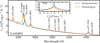 |
Fig. 1. Comparison of the optical luminosity of model r1w6b at 5 d after explosion and computed with either the nonmonotonic Sobolev solver or adopting homologous expansion along with the accurate blanketed solver in CMFGEN. See the discussion in Sect. 2. |
In this work, we have focused primarily on model r1w6b, but we also considered 2D ejecta built from variants where RCSM is 6 and 10 × 1014 cm (models r1w6[a,c]). Assuming homologous expansion, we performed CMFGEN calculations for the r1w6[a,b,c] models at times between 1.67–2.5 d up to 5–10 d after explosion. These epochs straddle the phase during which the photosphere is located in the unshocked CSM and eventually into the cold-dense shell (for a general overview of this evolution, see Dessart 2025a). In all cases presented here, the 2D ejecta built from these interaction models are prolate and have a moderate pole-to-equator density ratio of five. Furthermore, the variation with latitude as μ2 is progressive and moderate, thus, it excludes the extreme angular variations associated with jets and disks.
3. Polarization modeling results
Figure 2 shows the results from the 2D polarized radiative-transfer code LONG_POL for a 2D, prolate (ρpole/ρeq = 5) ejecta based on model r1w6b, for a 90-deg inclination, and from 2.5 to 10.0 d after explosion. The total flux, FI, displays emission lines with narrow cores and broad, symmetric, electron-scattering broadened wings for the first four epochs; whereas at the last epoch at 10.0 d, the total flux exhibits weak, blueshifted, Doppler broadened lines that are starting to show blueshifted, P Cygni absorptions. With the normalization of the total and polarized fluxes FI and FQ at 6300 Å, we can see that the slope of each is essentially identical. In other words, the overall continuum polarization is constant with wavelength. Across most lines, the polarized flux decreases, with a maximum reduction at the line cores; this indicates substantial depolarization of both line and continuum photons at these wavelengths.
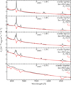 |
Fig. 2. Evolution of the total flux, FI, and the polarized flux, FQ (total flux multiplied by the percent polarization), computed with LONG_POL assuming a 2D, prolate ejecta based on model r1w6b (ρpole/ρeq = 5). Epochs cover from 2.5 to 10.0 d after explosion. Both fluxes are scaled to the inferred distance of SN 1998S, with an additional scaling for the total flux (see label) to match the magnitude of the polarized flux at 6300 Å (FQ flips sign at the last epoch). All fluxes have been rebinned at 6 Å. See the discussion in Sect. 3. |
The lower polarization across lines arises in part from the fact that all lines form exterior to the continuum-formation region and, thus, at lower electron-scattering optical depth (see second panel from top in Fig. A.1). The linear polarization arising from scattering with free electrons is therefore greater for continuum than for line photons. In the narrow line cores, we see photons that have undergone no frequency redistribution in wavelength (or in velocity space) as they traveled outwards from their original point of emission. We note that many of these “core” photons are emitted beyond the photosphere, at low electron-scattering optical depth, and would not be expected to exhibit a high level of polarization as a result. Thus, these line core photons experienced little or no scattering with free electrons and they are unpolarized. Furthermore, since the optical depth in some lines (e.g., Hα) is huge, the (polarized) continuum photons overlapping with the line cores suffer from absorption, leading to a narrow polarization dip in emission line cores.
The funnel-shaped profile observed in polarized flux across the lines indicates that the associated photons are depolarized (i.e., the polarized flux is below the level obtained by interpolating FQ from the adjacent continuum regions). This funnel shape arises because continuum photons originally emitted at λinit values that are not too far from the line’s rest wavelength, λc, will be absorbed by that line if they ever come within a few Doppler widths (say 10 km s−1) of λc. This eventuality may occur as photons randomly walk and scatter with free electrons in the CSM. The probability of this is greater as values of |λinit-λc| get smaller. In other words, the line cores act as a sink for neighboring (in λ-space) scattered continuum photons.
A number of subtleties are also apparent. For example, the C III/N III blend exhibits a weaker level of depolarization. These lines form deeper than Hα and thus closer to the region of continuum formation (see also Fig. A.1, and L00), but also through different processes (i.e., continuum fluorescence and dielectronic recombination). The polarization is found to be positive for the first four epochs and thereby aligned with the axis of symmetry. This results from an optical depth effect, suggesting that polarization is controlled primarily by the lower-density equatorial regions where the bulk of the radiation emerges, rather than the higher density regions where scattering is enhanced (see the discussion in Dessart & Hillier 2011). The polarization flips in sign at the last epoch (equivalent to a 90-deg rotation of the polarization angle) when the unshocked CSM has been fully swept up and the entire spectrum forms in the dense shell.
In this 2D prolate ejecta model with ρpole/ρeq = 5, the continuum polarization (which is essentially constant throughout the optical range) has a maximum value of 1.4% up to 4.17 d, dropping to 1.3% at 5.0 d and then further to 0.5% at 10.0 d. Hence, the presence of an extended unshocked CSM with a modest asymmetry can produce percent-level polarization at early times (as inferred in SNe 1998S or 2010jl), without invoking extreme explosion asymmetries (e.g., jets or disks). This result is also comparable to peak values obtained at the transition to the nebular phase of non-interacting Type II SNe (Leonard et al. 2015; Nagao et al. 2021). Modulations of RCSM do not affect the qualitative results obtained for r1w6b, but they do alter the values of the maximum polarization and its evolution in time (Appendix C). The equivalent 2D prolate ejecta based on model r1w6a (r1w6c) exhibit a maximum polarization of 1.0% (1.8%) and a decline at ∼5 d (∼10 d). Consequently, the Type II SNe with longer-lived IIn-like signatures should on average exhibit a greater level of polarization. Other parameters that may impact the polarization behavior include the CSM density or associated wind mass loss.
4. Comparison to spectropolarimetric observations of SN 1998S
We go on to compare our modeling results with the single-epoch spectropolarimetry of SN 1998S at ∼5 d post-explosion, presented and thoroughly discussed in L00. We chose to compare our models with these data since they remain (to our knowledge) the only optical spectropolarimetry obtained early enough to capture the strong ejecta-CSM interaction and with sufficient resolution (∼6 Å) to clearly reveal the spectropolarimetric behaviors of both the narrow- and broad-line features in an SN IIn.
The observed data of SN 1998S from L00 present a high degree (∼2%) of wavelength-independent continuum polarization across the observed spectral range (4314–6850 Å) and sharp depolarizations across all strong emission lines (see Fig. 3, as well as the “ISP2” panel of Fig. 4 in this work). To convert these observed data into intrinsic polarization that can be directly compared with our models, we must first determine a plausible value of the ISP.
We present the observed data of SN 1998S in the Stokes q − u plane in Fig. 3. In this representation, the black circles clustering around [q, u] ≈ [−0.9%, −1.7%] arise from the continuum regions; the red and green circles specifically correspond to the broad wings and narrow core spectral regions of Hα.
This presentation enables immediate identification of an interesting fact: The broad wings and narrow core photons “point” along different directions in the Stokes q − u plane. Indeed, L00 used this to derive two different ISP possibilities, one with the assumption of unpolarized photons in the broad wings of strong lines and one under the assumption of unpolarized photons contributed solely by the narrow emission lines; these choices are indicated by the points identified in Fig. 3 as “ISP-L00” and “ISP4.”
In this regard, we are guided by the modeling results of the previous section and the prediction that the spectral region corresponding specifically to the narrow-line core of strong emission features (i.e., Hα) should consist not only of intrinsically unpolarized narrow-line photons – but also a significantly (if not completely) depolarized underlying continuum at these wavelengths. This presents to us a new range of ISP choices, for which the bounds can be easily established. First, if the narrow-line core of Hα is assumed to have zero intrinsic polarization (i.e., unpolarized line photons and completely depolarized underlying continuum), then the ISP must lie simply at the location of the tip of the narrow Hα line in the q − u plane; this is indicated by “ISP1” in Fig. 3. At the other extreme lies the result that obtains if we assume only unpolarized narrow-line photons and no depolarization of the underlying continuum photons; this is indicated by “ISP4” in Fig. 3. The line connecting these two points then spans the range of allowable ISP values under different assumptions about the degree of depolarization of the underlying continuum. One such example is “ISP3” located at [q, u] = [0.55%, 0.40%], chosen specifically to best fit the depolarization at Hα found by model r1w6b at 5 d. Interestingly, the origin is also an allowable ISP choice and so, we also ought to consider that possibility and label that point “ISP2.”
When the four ISP choices labeled in Fig. 3 are removed from the SN 1998S data, they yield the intrinsic polarizations shown in the bottom panels of Fig. 4. While the inferred overall level of continuum polarization changes drastically with the ISP choice, it is notable that the basic features of the resulting spectropolarimetry do not. Specifially, a high level of wavelength-independent continuum polarization with “funnel-shaped” depolarizations is evident throughout the strong line features. The level of depolarization across lines is best matched by choices ISP[1,2,3], which imply an intrinsic continuum polarization in SN 1998S of ∼2%; this is in rough agreement with our 2D prolate ejecta model with ρpole/ρeq = 5. Choice ISP4 implies a high intrinsic polarization but a very weak depolarization within lines, which is not as well matched by our models. As noted by L00, such a high degree of ISP also strains the allowable values from reddening considerations. Thus, we arrive at the conclusion that the SN 1998S spectropolarimetry likely suffered little ISP contamination; in fact, assuming zero ISP produces results in as good agreement with our model predictions as any other.
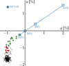 |
Fig. 3. Polarization data in the q − u plane for SN 1998S at ∼5 d after explosion, from L00. Photons with wavelengths corresponding to the broad wings and narrow-line core of the Hα flux profile are indicated with red and green circles, respectively. Each point represents a bin 10 Å wide, except for the green circles, which are binned at 2 Å for enhanced resolution. The blue line spans the range of potential ISP choices derived from different assumptions about the extent of depolarization in the narrow-line core region of Hα. The blue squares indicate four specific choices of ISP discussed in the text, which yield the inferred intrinsic polarizations displayed in the bottom panels of Fig. 4. See Sect. 4 for a discussion. |
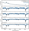 |
Fig. 4. Comparison of the spectropolarimetric observations of SN 1998S at 5 d after explosion with the counterparts obtained with LONG_POL assuming a 2D, prolate ejecta (ρpole/ρeq = 5) based on model r1w6b at 5 d. The observer’s inclination relative to the axis of symmetry is 90 deg. Four ISP choices are shown, corresponding to ISP[1,2,3,4] indicated in Fig. 3. Note: “ISP2” represents the observed data, with no ISP removed (the residuals for each case are shown in Fig. C.1). Observations have been corrected for a recession velocity of 840 km s−1 and a reddening E(B − V) of 0.11 mag. Model spectra have been smoothed and rebinned to 6 Å to match the resolution of the observations. See Sect. 4 for a discussion. |
As the data in the q − u plane do not lie perfectly along a straight line (Fig. 3), the ejecta associated with SN1998S must exhibit departures from axial symmetry. The small degree of polarization angle rotation across the broad emission lines is not presently captured by our models and is a limitation of the imposed axisymmetry in LONG_POL. The modeling of such features requires 3D polarized radiative-transfer and is left to a future work.
5. Conclusion
We have presented an end-to-end modeling of RSG stars exploding inside an asymmetric CSM. The models are based on 1D radiation-hydrodynamics calculations with HERACLES of the ejecta interaction with the CSM, the post-treatment of multiepoch snapshots with the 1D radiative transfer code CMFGEN, and, finally, the 2D polarized radiative transfer with LONG_POL. The main limitation of our work is the incomplete physical consistency, since asymmetry is only introduced at the last modeling stage with LONG_POL. Another adjustment is the enforcement of homologous expansion, as currently required by LONG_POL, although we show that this modification is acceptable (see Sect. 2 and Appendix A). We selected the interaction model r1w6b (and offshoots r1w6[a,c]), presented and confronted with the results on SN 2023ixf from Jacobson-Galán et al. (2023).
Adopting a simple, depth-independent, latitudinal scaling of the density and assuming suitable scaling relations for the opacities and emissivities computed with CMFGEN for the 1D model r1w6b, we modeled the spectropolarimetry of 2D prolate ejecta with a pole-to-equator density ratio of 5. In those H-rich, ionized environments where the electron-scattering opacity dominates throughout, apart from the line cores, the polarization is essentially constant with wavelength, with the exception of funnel-shaped depolarizations across lines. The lower polarization across lines follows from the formation of lines exterior to the continuum and, thus, at a lower electron-scattering optical depth; however, the additional depolarization is caused by the disappearance of continuum photons that wander into λ-space too close to highly-absorbing line cores. Our simulations with a fixed, depth-independent asymmetry suggest the overall polarization should remain constant for several days in SNe II with CSM interaction before dropping and eventually flipping sign, as the shock emerges from the CSM. For a fixed CSM density, models with more compact (extended) CSM exhibit a lower (greater) maximum polarization with a more (less) rapid evolution.
Our finding that the narrow line cores ought to exhibit some level of depolarization was used to set constraints on the ISP of SN 1998S, leading to the conclusion that the intrinsic polarization of SN 1998S is ∼2%. Our models replicate the wavelength independence of the continuum polarization, with the funnel-shaped depolarization across lines. This similarity lends support to the essential ansatz of our models and the numerical approach. As discussed in Sect. 3 (see also results for models r1w6[a,c] in Appendix C), by tweaking a few input parameters (e.g., RCSM, ρpole/ρeq, etc.), we could, in principle, provide better fits to the actual levels of (even temporally changing) continuum polarization for objects where the ISP is more tightly constrained than is the case for SN 1998S. Overall, our methodology extended here to include spectropolarimetry offers a means to model and constrain the properties of the growing sample of Type II SNe with CSM interaction like 2023ixf and better understand the origin of pre-SN mass loss.
Acknowledgments
This work was granted access to the HPC resources of TGCC under the allocation 2023 – A0150410554 on Irene-Rome made by GENCI, France. D.C.L. acknowledges support from NSF grant AST-2010001, under which part of this research was carried out. D.J.H. gratefully acknowledges support through NASA astro-physical theory grant 80NSSC20K0524.
References
- Brown, J. C., & McLean, I. S. 1977, A&A, 57, 141 [NASA ADS] [Google Scholar]
- Bruch, R. J., Gal-Yam, A., Schulze, S., et al. 2021, ApJ, 912, 46 [NASA ADS] [CrossRef] [Google Scholar]
- Bruch, R. J., Gal-Yam, A., Yaron, O., et al. 2023, ApJ, 952, 119 [NASA ADS] [CrossRef] [Google Scholar]
- Chandrasekhar, S. 1960, Radiative Transfer (New York: Dover) [Google Scholar]
- Chugai, N. N. 2001, MNRAS, 326, 1448 [NASA ADS] [CrossRef] [Google Scholar]
- Chugai, N. N., Blinnikov, S. I., Fassia, A., et al. 2002, MNRAS, 330, 473 [NASA ADS] [CrossRef] [Google Scholar]
- Dessart, L. 2025a, Encyclopedia of Astrophysics, 1st Edn. in press, [arXiv:2405.04259] [Google Scholar]
- Dessart, L. 2025b, A&A, 694, A132 [NASA ADS] [CrossRef] [EDP Sciences] [Google Scholar]
- Dessart, L., & Hillier, D. J. 2011, MNRAS, 415, 3497 [Google Scholar]
- Dessart, L., Hillier, D. J., Gezari, S., Basa, S., & Matheson, T. 2009, MNRAS, 394, 21 [NASA ADS] [CrossRef] [Google Scholar]
- Dessart, L., Audit, E., & Hillier, D. J. 2015, MNRAS, 449, 4304 [Google Scholar]
- Dessart, L., Hillier, D. J., & Audit, E. 2017, A&A, 605, A83 [NASA ADS] [CrossRef] [EDP Sciences] [Google Scholar]
- Dessart, L., Hillier, D. J., & Leonard, D. C. 2021a, A&A, 651, A10 [NASA ADS] [CrossRef] [EDP Sciences] [Google Scholar]
- Dessart, L., Leonard, D. C., Hillier, D. J., & Pignata, G. 2021b, A&A, 651, A19 [NASA ADS] [CrossRef] [EDP Sciences] [Google Scholar]
- Fransson, C., Ergon, M., Challis, P. J., et al. 2014, ApJ, 797, 118 [Google Scholar]
- Fuller, J. 2017, MNRAS, 470, 1642 [NASA ADS] [CrossRef] [Google Scholar]
- Fuller, J., & Tsuna, D. 2024, Open J. Astrophys., 7, 47 [CrossRef] [Google Scholar]
- González, M., Audit, E., & Huynh, P. 2007, A&A, 464, 429 [Google Scholar]
- Hillier, D. J. 1987, ApJS, 63, 965 [NASA ADS] [CrossRef] [Google Scholar]
- Hillier, D. J. 1994, A&A, 289, 492 [NASA ADS] [Google Scholar]
- Hillier, D. J. 1996, A&A, 308, 521 [NASA ADS] [Google Scholar]
- Hillier, D. J., & Dessart, L. 2012, MNRAS, 424, 252 [CrossRef] [Google Scholar]
- Hillier, D. J., & Miller, D. L. 1998, ApJ, 496, 407 [NASA ADS] [CrossRef] [Google Scholar]
- Hoflich, P. 1991, A&A, 246, 481 [NASA ADS] [Google Scholar]
- Jacobson-Galán, W. V., Dessart, L., Margutti, R., et al. 2023, ApJ, 954, L42 [CrossRef] [Google Scholar]
- Jacobson-Galán, W. V., Dessart, L., Davis, K. W., et al. 2024, ApJ, 970, 189 [CrossRef] [Google Scholar]
- Leonard, D. C., Filippenko, A. V., Barth, A. J., & Matheson, T. 2000, ApJ, 536, 239 [Google Scholar]
- Leonard, D. C., Dessart, L., Pignata, G., et al. 2015, IAU Gen. Assembly, 29, 2255774 [NASA ADS] [Google Scholar]
- Leonard, D. C., Dessart, L., Hillier, D. J., et al. 2021, ApJ, 921, L35 [NASA ADS] [CrossRef] [Google Scholar]
- Mauerhan, J., Williams, G. G., Smith, N., et al. 2014, MNRAS, 442, 1166 [NASA ADS] [CrossRef] [Google Scholar]
- McCall, M. L. 1984, MNRAS, 210, 829 [Google Scholar]
- Nagao, T., Patat, F., Taubenberger, S., et al. 2021, MNRAS, 505, 3664 [NASA ADS] [CrossRef] [Google Scholar]
- Niemela, V. S., Ruiz, M. T., & Phillips, M. M. 1985, ApJ, 289, 52 [NASA ADS] [CrossRef] [Google Scholar]
- Patat, F., Taubenberger, S., Benetti, S., Pastorello, A., & Harutyunyan, A. 2011, A&A, 527, L6 [NASA ADS] [CrossRef] [EDP Sciences] [Google Scholar]
- Pessi, T., Cartier, R., Hueichapan, E., et al. 2024, A&A, 688, L28 [NASA ADS] [CrossRef] [EDP Sciences] [Google Scholar]
- Quataert, E., & Shiode, J. 2012, MNRAS, 423, L92 [NASA ADS] [CrossRef] [Google Scholar]
- Schlegel, E. M. 1990, MNRAS, 244, 269 [NASA ADS] [Google Scholar]
- Shivvers, I., Groh, J. H., Mauerhan, J. C., et al. 2015, ApJ, 806, 213 [NASA ADS] [CrossRef] [Google Scholar]
- Singh, A., Teja, R. S., Moriya, T. J., et al. 2024, ApJ, 975, 132 [CrossRef] [Google Scholar]
- Smith, N., Pearson, J., Sand, D. J., et al. 2023, ApJ, 956, 46 [NASA ADS] [CrossRef] [Google Scholar]
- Soker, N. 2021, ApJ, 906, 1 [Google Scholar]
- Vasylyev, S. S., Yang, Y., Filippenko, A. V., et al. 2023, ApJ, 955, L37 [NASA ADS] [CrossRef] [Google Scholar]
- Wang, L., & Wheeler, J. C. 2008, ARA&A, 46, 433 [Google Scholar]
- Wang, L., Howell, D. A., Höflich, P., & Wheeler, J. C. 2001, ApJ, 550, 1030 [NASA ADS] [CrossRef] [Google Scholar]
- Woosley, S. E., & Heger, A. 2015, ApJ, 810, 34 [NASA ADS] [CrossRef] [Google Scholar]
- Wu, S. C., & Fuller, J. 2022, ApJ, 940, L27 [NASA ADS] [CrossRef] [Google Scholar]
- Yaron, O., Perley, D. A., Gal-Yam, A., et al. 2017, Nat. Phys., 13, 510 [NASA ADS] [CrossRef] [Google Scholar]
- Yoon, S.-C., & Cantiello, M. 2010, ApJ, 717, L62 [NASA ADS] [CrossRef] [Google Scholar]
- Zhang, T., Wang, X., Wu, C., et al. 2012, AJ, 144, 131 [NASA ADS] [CrossRef] [Google Scholar]
Appendix A: The assumption of homologous expansion in CMFGEN simulations of interacting supernovae
We show some results from the CMFGEN calculation, assuming homologous expansion in Fig. A.1 and using the model r1w6b (RCSM= 8× 1014 cm) – this model was found by Jacobson-Galán et al. (2023) to yield a satisfactory match to the photometric and spectroscopic evolution of SN 2023ixf, a close analog of SN 1998S (model r1w6b is derived from model r1w6 of Dessart et al. (2017), which has been extensively used in the SN community). The time is 5 d after the first detection.
Looking at the velocity structure first, we see that the original, nonmonotonic velocity and the new (“fudged”) homologous velocity (bottom panel of Fig. A.1) differ significantly. By assuming homologous expansion, the fast inner regions are now the slowest, while the originally slow outer CSM regions are now the fastest. The unadulterated velocities differ from the initial velocities because of the radiative acceleration of the unshocked CSM (see simulation results for this phenomenon in Dessart et al. 2017 and Dessart 2025b; see also Chugai et al. 2002). Here, in the HERACLES calculation, the entire CSM is predicted to move at a velocity greater than 200 km s−1 and as fast as 300 km s−1 at the photosphere location at 5 d. Such relatively large velocities suggest that a resolution of 300 km s−1 is not so bad for spectropolarimetric observations of interacting SNe (as obtained by L00 for SN 1998S).
These offsets have, however, a moderate impact for what concerns us. First, the inner, fast-moving layers are at high optical depth and, thus, contribute negligibly to the emergent flux (both are shown in the second panel from top in Fig. A.1). The outer CSM regions are of low density and low optical depth and will thus have a weak impact, essentially limited to the narrow emission line cores. Because these velocities are still small, they are typically unresolved in spectropolarimetric observations – our models will simply overestimate the width of this narrow, line core emission by a factor of about two. The bulk of the spectrum forms between optical depth 0.1 and 10 (i.e., around the photosphere; see the cumulative fractional luminosity  versus depth in Fig. A.1, second panel from top), where the original and the modified velocities are similar by design. Electron scattering is the dominant line broadening mechanism at such times and in those regions; since we are not concerned with the information at the 100 km s−1 scale that are only available in high-resolution spectra, this slight change in material velocity is unimportant.
This adjustment of the original nonmonotonic velocity into a homologous flow leads to different velocities at different epochs or in different models. While we set V = R/t and t = Rphot/Vphot in all cases, the quantities Rphot and Vphot are specific of each HERACLES snapshot for each model studied. Obviously, this “homologous” time does not correspond to any physical time for either the ejecta, the CSM, or the interacting SN; however, this time plays no role in the steady-state radiative transfer to be performed.
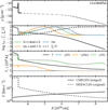 |
Fig. A.1. Illustration of ejecta and radiative properties of model r1w6b at 5 d after explosion, as computed by HERACLES and CMFGEN. From top to bottom, we show the variation with radius of the mass density (dots correspond to the CMFGEN radial grid) ; the electron-scattering optical depth τes (solid black curve) together with the regions of formation of Hα, He II 4685.7 Å, and N III 4640.6 Å (denoted |


Appendix B: Polarized radiative transfer with LONG_POL
For completeness, we summarize the nomenclature and sign conventions adopted in LONG_POL and also presented by Dessart & Hillier (2011). We assume that the polarization is produced by electron scattering. The scattering of electromagnetic radiation by electrons is described by the dipole or Rayleigh scattering phase matrix. To describe the “observed” model polarization we adopted the Stokes parameters I, Q, U, and V (Chandrasekhar 1960). Since we are dealing with electron scattering, the polarization is linear and the V Stokes parameter is identically zero. For clarity, IQ and IU refer to the polarization of the specific intensity, and FQ and FU refer to the polarization of the observed flux.
For consistency with the earlier work of Hillier (1994, 1996) we chose a right-handed set of unit vectors (ζX, ζY, ζW). Without loss of generality the axisymmetric source is centered at the origin of the coordinate system with its symmetry axis lying along ζW, ζY is in the plane of the sky and the observer is located in the XW plane.
We take FQ to be positive when the polarization is parallel to the symmetry axis (or, more consistently, parallel to the projection of the symmetry axis on the sky) and negative when it is perpendicular to it. With our choice of coordinate system, and since the SN ejecta are left-right symmetric about the XW plane, FU is zero by construction. This must be the case since symmetry requires that the polarization can only be parallel, or perpendicular to, the axis of symmetry. For a spherical source, FQ is also identically zero.
I(ρ, δ), IQ(ρ, δ), and IU(ρ, δ) refer to the observed intensities on the plane of the sky. Here, IQ is positive when the polarization is parallel to the radius vector, and negative when it is perpendicular. In the plane of the sky we define a set of polar coordinates (ρ, δ) with the angle δ measured anti-clockwise from ζY. The polar coordinate, ρ, can also be thought of as the impact parameter of an observer’s ray. We also use the axes defined by the polar coordinate system to describe the polarization. FI is obtained from I(ρ, δ) using
 (B.1)
(B.1)
where dA = ρdδdρ. Since ζρ is rotated by an angle δ anticlockwise from ζY, FQ is given by
![Mathematical equation: $$ \begin{aligned} F_Q = {-2 \over d^2} \int _0^{\rho _{\rm max}} \int _{-\pi /2}^{\pi /2} \left[ I_Q(\rho ,\delta ) \cos 2\delta + I_U(\rho ,\delta ) \sin 2\delta \right] \, dA \,. \end{aligned} $$](/articles/aa/full_html/2025/04/aa52327-24/aa52327-24-eq6.gif) (B.2)
(B.2)
In a spherical system, IQ is independent of δ, and IU is identically zero.
The percentage polarization Pλ is defined as 100|FQ/FI|, where we have dropped the λ subscript of the fluxes for clarity.
In this paper and for brevity, we report mostly on the maximum polarization obtained for a 90-deg inclination angle i. The variation with i has been discussed in previous studies and may deviate from a simple sin2i dependence if optical-depth effects are present (Dessart et al. 2021a,b).
Appendix C: Additional models and illustrations
Figure C.1 shows the residuals of the percentage polarization between observation and models shown in Fig. 4. Figures C.2 and C.3 show a counterpart of Fig. 2 for the simulation results of model r1w6a and r1w6c and discussed briefly in Sect. 2. These two additional models differ from model r1w6b in the value of RCSM, which is 6 and 10×1014 cm, respectively. Our simulations indicate that the polarization is maximum when the shock is embedded within the CSM, and that it is greater for greater RCSM. Despite the modest pole-to-equator density ratio of five, model r1w6c has a maximum continuum polarization of nearly 2 %.
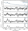 |
Fig. C.1. Counterpart of Fig. 4 but showing the residuals (i.e., Pobs − Pmod, with the same scaling as in Fig. 4) rather than the polarization for the observations of SN 1998S at 5 d and the model with ISP choices 1, 2, 3, and 4 (see also Fig. 3). The residuals have been smoothed with a gaussian kernel (FWHM of 10 Å). |
All Figures
|
Fig. 1. Comparison of the optical luminosity of model r1w6b at 5 d after explosion and computed with either the nonmonotonic Sobolev solver or adopting homologous expansion along with the accurate blanketed solver in CMFGEN. See the discussion in Sect. 2. |
| In the text | |
|
Fig. 2. Evolution of the total flux, FI, and the polarized flux, FQ (total flux multiplied by the percent polarization), computed with LONG_POL assuming a 2D, prolate ejecta based on model r1w6b (ρpole/ρeq = 5). Epochs cover from 2.5 to 10.0 d after explosion. Both fluxes are scaled to the inferred distance of SN 1998S, with an additional scaling for the total flux (see label) to match the magnitude of the polarized flux at 6300 Å (FQ flips sign at the last epoch). All fluxes have been rebinned at 6 Å. See the discussion in Sect. 3. |
| In the text | |
|
Fig. 3. Polarization data in the q − u plane for SN 1998S at ∼5 d after explosion, from L00. Photons with wavelengths corresponding to the broad wings and narrow-line core of the Hα flux profile are indicated with red and green circles, respectively. Each point represents a bin 10 Å wide, except for the green circles, which are binned at 2 Å for enhanced resolution. The blue line spans the range of potential ISP choices derived from different assumptions about the extent of depolarization in the narrow-line core region of Hα. The blue squares indicate four specific choices of ISP discussed in the text, which yield the inferred intrinsic polarizations displayed in the bottom panels of Fig. 4. See Sect. 4 for a discussion. |
| In the text | |
|
Fig. 4. Comparison of the spectropolarimetric observations of SN 1998S at 5 d after explosion with the counterparts obtained with LONG_POL assuming a 2D, prolate ejecta (ρpole/ρeq = 5) based on model r1w6b at 5 d. The observer’s inclination relative to the axis of symmetry is 90 deg. Four ISP choices are shown, corresponding to ISP[1,2,3,4] indicated in Fig. 3. Note: “ISP2” represents the observed data, with no ISP removed (the residuals for each case are shown in Fig. C.1). Observations have been corrected for a recession velocity of 840 km s−1 and a reddening E(B − V) of 0.11 mag. Model spectra have been smoothed and rebinned to 6 Å to match the resolution of the observations. See Sect. 4 for a discussion. |
| In the text | |
|
Fig. A.1. Illustration of ejecta and radiative properties of model r1w6b at 5 d after explosion, as computed by HERACLES and CMFGEN. From top to bottom, we show the variation with radius of the mass density (dots correspond to the CMFGEN radial grid) ; the electron-scattering optical depth τes (solid black curve) together with the regions of formation of Hα, He II 4685.7 Å, and N III 4640.6 Å (denoted |
| In the text | |
|
Fig. C.1. Counterpart of Fig. 4 but showing the residuals (i.e., Pobs − Pmod, with the same scaling as in Fig. 4) rather than the polarization for the observations of SN 1998S at 5 d and the model with ISP choices 1, 2, 3, and 4 (see also Fig. 3). The residuals have been smoothed with a gaussian kernel (FWHM of 10 Å). |
| In the text | |
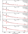 |
Fig. C.2. Same as Fig. 2 but for model r1w6a and from 1.67 to 5.00 d. |
| In the text | |
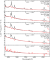 |
Fig. C.3. Same as Fig. 2 but for model r1w6c |
| In the text | |
Current usage metrics show cumulative count of Article Views (full-text article views including HTML views, PDF and ePub downloads, according to the available data) and Abstracts Views on Vision4Press platform.
Data correspond to usage on the plateform after 2015. The current usage metrics is available 48-96 hours after online publication and is updated daily on week days.
Initial download of the metrics may take a while.